III BCA DATAMINING NOTES UNIT III - WordPress.com
16
HINDUSTHAN COLLEGE OF ARTS AND SCIENCE AUTONOMOUS (Affiliated to Bharathiar University) Behind Nava India, Coimbatore - 641028. DEPARTMENT OF COMPUTER APPLICATIONS (BCA) III BCA DATAMINING NOTES – UNIT III Prepared By Dr.Sasikala,Asst Prof Mr.Aravind,Asst Prof Mrs.Saranya,Asst Prof
Transcript of III BCA DATAMINING NOTES UNIT III - WordPress.com

HINDUSTHAN COLLEGE OF ARTS AND SCIENCE AUTONOMOUS
(Affiliated to Bharathiar University)
Behind Nava India, Coimbatore - 641028.
DEPARTMENT OF COMPUTER APPLICATIONS (BCA)
III BCA
DATAMINING NOTES – UNIT III
Prepared By
Dr.Sasikala,Asst Prof
Mr.Aravind,Asst Prof
Mrs.Saranya,Asst Prof

UNIT III
Clustering: Introduction – Similarity and Distance Measures – Outliers – Hierarchical Algorithms - Partitional Algorithms. Association
rules: Introduction - large item sets - basic algorithms – parallel & distributed algorithms – comparing approaches- incremental rules –
advanced association rules techniques – measuring the quality of rules.
CLUSTERING
INTRODUCTION
Clustering Example
Clustering Houses
Clustering vs. Classification
No prior knowledge
o Number of clusters
o Meaning of clusters
Unsupervised learning
Clustering Issues
Outlier handling
Dynamic data
Interpreting results
Evaluating results
Number of clusters
Data to be used
Scalability
Impact of Outliers on Clustering

Clustering Problem: Definition
Given a database D={t1,t2,…,tn} of tuples and an integer value k, the Clustering Problem is to define a mapping f:Dg{1,..,k} where
each ti is assigned to one cluster Kj, 1<=j<=k. A Cluster, Kj, contains precisely those tuples mapped to it.Unlike classification problem,
clusters are not known a priori.
Types of Clustering
Hierarchical – Nested set of clusters created.
Partitional – One set of clusters created.
Incremental – Each element handled one at a time.
Simultaneous – All elements handled together.
Overlapping/Non-overlapping
Clustering Approaches
Cluster Parameters
SIMILARITY AND DISTANCE MEASURES Since clustering is the grouping of similar instances/objects, some sort of measure that can determine whether two objects are
similar or dissimilar is required. There are two main type of measures used to estimate this relation: distance measures and similarity
measures.
Many clustering methods use distance measures to determine the similarity or dissimilarity between any pair of objects. It is useful
to denote the distance between two instances xi and xj as: d(xi ,xj). A valid distance measure should be symmetric and obtains its minimum
value (usually zero) in case of identical vectors. The distance measure is called a metric distance measure if it also satisfies the following
properties:
1. Triangle inequality d(xi,xk) <= d(xi,xj) + d(xj,xk) Vxi,xj,xk E S.
2. d(xi,xj) => xi = xj Vxi,xj E S.
An alternative concept to that of the distance is the similarity functions(xi; xj) that compares the two vectors xi and xj (Duda et al.,
2001). This function should be symmetrical (namely s(xi; xj) = s(xj; xi)) and have a large value when xi and xj are somehow “similar” and
constitute the largest value for identical vectors.
A similarity function where the target range is [0,1] is called a dichotomous similarity function. In fact, the methods described in the
previous sections for calculating the “distances” in the case of binary and nominal attributes may be considered as similarity functions,

rather than distances.
OUTLIERS Very often, there exist data objects that do not comply with the general behavior or model of the data. Such data objects, which are
grossly different from or inconsistent with the remaining set of data are called Outliers.
Outlier detection and analysis is an interesting data mining task referred to as outlier mining or outlie analysis.
Distance Between Clusters
Single Link: smallest distance between points
Complete Link: largest distance between points
Average Link: average distance between points
Centroid: distance between centroids
HIERARCHICAL CLUSTERING
Clusters are created in levels actually creating sets of clusters at each level.
1. Agglomerative
Initially each item in its own cluster
Iteratively clusters are merged together
Bottom Up
2. Divisive
Initially all items in one cluster
Large clusters are successively divided
Top Down
Hierarchical Algorithms
Single Link
MST Single Link
Complete Link
Average Link
Dendrogram
Dendrogram: a tree data structure which illustrates hierarchical clustering techniques.
Each level shows clusters for that level.
Leaf – individual clusters
Root – one cluster
A cluster at level i is the union of its children clusters at level i+1.
Levels of Clustering

Agglomerative Example
A B C D E
A 0 1 2 2 3
B 1 0 2 4 3
C 2 2 0 1 5
D 2 4 1 0 3
E 3 3 5 3 0
MST Example
Agglomerative Algorithm

Single Link
View all items with links (distances) between them. Finds maximal connected components in this graph. Two clusters are merged if
there is at least one edge which connects them. Uses threshold distances at each level. Could be agglomerative or divisive.
Single Link Clustering
PARTITIONING ALGORITHMS
Partitional Clustering Nonhierarchical
Creates clusters in one step as opposed to several steps.Since only one set of clusters is output, the user normally has to input the desired
number of clusters, k. Usually deals with static sets.

MST Algorithm
Squared Error
Minimized squared error
Squared Error Algorithm
K-Means
Initial set of clusters randomly chosen. Iteratively, items are moved among sets of clusters until the desired set is reached. High
degree of similarity among elements in a cluster is obtained. Given a cluster Ki={ti1,ti2,…,tim}, the cluster mean is mi = (1/m)(ti1 + … +
tim)
Example
Given: {2,4,10,12,3,20,30,11,25}, k=2
Randomly assign means: m1=3,m2=4
K1={2,3}, K2={4,10,12,20,30,11,25}, m1=2.5,m2=16
K1={2,3,4},K2={10,12,20,30,11,25}, m1=3,m2=18
K1={2,3,4,10},K2={12,20,30,11,25}, m1=4.75,m2=19.6
K1={2,3,4,10,11,12},K2={20,30,25}, m1=7,m2=25
Stop as the clusters with these means are the same.

Nearest Neighbor
Items are iteratively merged into the existing clusters that are closest. Incremental Threshold, t, used to determine if items are
added to existing clusters or a new cluster is
created.
PAM

Partitioning Around Medoids (PAM) (K-Medoids) Handles outliers well. Ordering of input does not impact results. Does not scale
well. Each cluster represented by one item, called the medoid. Initial set of k medoids randomly chosen.
PAM Cost Calculation
At each step in algorithm, medoids are changed if the overall cost is improved. Cjih – cost change for an item tj associated with swapping
medoid ti with non-medoid th.
BEA
Bond Energy Algorithm
Database design (physical and logical)
Vertical fragmentation
Determine affinity (bond) between attributes based on common usage.
Algorithm outline:
o Create affinity matrix
o Convert to BOND matrix
o Create regions of close bonding

Genetic Algorithm Example
{A,B,C,D,E,F,G,H}
Randomly choose initial solution:
{A,C,E} {B,F} {D,G,H} or
10101000, 01000100, 00010011
Suppose crossover at point four and choose 1st and 3rd individuals:
10100011, 01000100, 00011000
What should termination criteria be?
ASSOCIATION RULES
INTRODUCTION
Associations and Item-sets:
An association is a rule of the form: if X then Y. It is denoted as X Y
Example:
If India wins in cricket, sales of sweets go up.
For any rule if X Y Y X, then X and Y are called an “interesting item-set”.
Example:
People buying school uniforms in June also buy school bags
(People buying school bags in June also buy school uniforms)
Support and Confidence:
The support for a rule R is the ratio of the number of occurrences of R, given all occurrences of all rules. The confidence of a rule X
Y, is the ratio of the number of
occurrences of Y given X, among all other occurrences given X.
Support for {Bag, Uniform} = 5/10 = 0.5
Confidence for Bag Uniform = 5/8 = 0.625
LARGE ITEM SETS
Set of items: I={I1,I2,…,Im}
Transactions: D={t1,t2, …, tn}, tjÍ I
Itemset: {Ii1,Ii2, …, Iik} Í I
Support of an itemset: Percentage of transactions which contain that itemset.
Large (Frequent) itemset: Itemset whose number of occurrences is above a threshold.
I = { Beer, Bread, Jelly, Milk, PeanutButter}
Support of {Bread,PeanutButter} is 60%
Association Rule (AR): implication X Þ Y where X,Y Í I and X Ç Y = ;
Support of AR (s) X Þ Y: Percentage of transactions that contain X ÈY
Confidence of AR (a) X Þ Y: Ratio of number of transactions that contain X È Y to the number that contain X

Given a set of items I={I1,I2,…,Im} and a database of transactions D={t1,t2, …, tn} where ti={Ii1,Ii2, …, Iik} and Iij Î I, the Association
Rule Problem is to identify all association rules X Þ Y with a minimum support and confidence.
BASIC ALGORITHMS
Apriori ALGORITHM
Large Itemset Property:
Any subset of a large itemset is large.
Contrapositive:
If an itemset is not large, none of its supersets are large.
Large Itemset Property
Apriori Algorithm
C1 = Itemsets of size one in I;
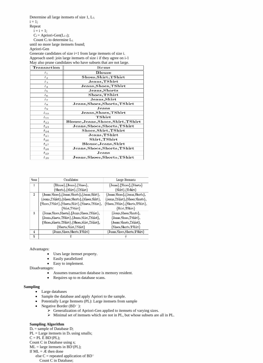
Determine all large itemsets of size 1, L1;
i = 1;
Repeat
i = i + 1;
Ci = Apriori-Gen(Li-1);
Count Ci to determine Li;
until no more large itemsets found;
Apriori-Gen
Generate candidates of size i+1 from large itemsets of size i.
Approach used: join large itemsets of size i if they agree on i-1
May also prune candidates who have subsets that are not large.
Advantages:
Uses large itemset property.
Easily parallelized
Easy to implement.
Disadvantages:
Assumes transaction database is memory resident.
Requires up to m database scans.
Sampling
Large databases
Sample the database and apply Apriori to the sample.
Potentially Large Itemsets (PL): Large itemsets from sample
Negative Border (BD - ):
Generalization of Apriori-Gen applied to itemsets of varying sizes.
Minimal set of itemsets which are not in PL, but whose subsets are all in PL.
Sampling Algorithm
Ds = sample of Database D;
PL = Large itemsets in Ds using smalls;
C = PL È BD-(PL);
Count C in Database using s;
ML = large itemsets in BD-(PL);
If ML = Æ then done
else C = repeated application of BD-;
Count C in Database;

Example:
Find AR assuming s = 20%
Ds = { t1,t2}
Smalls = 10%
PL = {{Bread}, {Jelly}, {PeanutButter}, {Bread,Jelly}, {Bread,PeanutButter}, {Jelly, PeanutButter}, {Bread,Jelly,PeanutButter}}
BD-(PL)={{Beer},{Milk}}
ML = {{Beer}, {Milk}}
Repeated application of BD- generates all remaining itemsets
Advantages:
Reduces number of database scans to one in the best case and two in worst.
Scales better.
Disadvantages:
Potentially large number of candidates in second pass
Partitioning
Divide database into partitions D1,D2,…,Dp . Apply Apriori to each partition. Any large itemset must be large in at least one
partition.
Algorithm
Divide D into partitions D1,D2,…,Dp;
For I = 1 to p do
Li = Apriori(Di);
C = L1 È … È Lp;
Count C on D to generate L;
Partitioning Example
Advantages:
Adapts to available main memory
Easily parallelized
Maximum number of database scans is two.
Disadvantages:
May have many candidates during second scan.
PARALLEL AND DISTRIBUTED ALGORITHMS
Parallelizing AR Algorithms
Based on Apriori
Techniques differ:
What is counted at each site
How data (transactions) are distributed
Data Parallelism
Data partitioned
Count Distribution Algorithm
Task Parallelism
Data and candidates partitioned
Data Distribution Algorithm
Count Distribution Algorithm(CDA)
Place data partition at each site.
In Parallel at each site do
C1 = Itemsets of size one in I;
Count C1;
Broadcast counts to all sites;
Determine global large itemsets of size 1, L1;

i = 1;
Repeat
i = i + 1;
Ci = Apriori-Gen(Li-1);
Count Ci;
Broadcast counts to all sites;
Determine global large itemsets of size i, Li;
until no more large itemsets found;
CDA Example
Data Distribution Algorithm(DDA)
Place data partition at each site.
In Parallel at each site do
Determine local candidates of size 1 to count;
Broadcast local transactions to other sites;
Count local candidates of size 1 on all data;
Determine large itemsets of size 1 for local candidates;
Broadcast large itemsets to all sites;
Determine L1;
i = 1;
Repeat
i = i + 1;
Ci = Apriori-Gen(Li-1);
Determine local candidates of size i to count;
Count, broadcast, and find Li;
until no more large itemsets found;
COMPARING APPROACHES Comparing AR Techniques
Target
Type
Data Type
Data Source
Technique
Itemset Strategy and Data Structure
Transaction Strategy and Data Structure
Optimization

Architecture
Parallelism Strategy
INCREMENTAL ASSOCIATION RULES
Generate Association Rules in a dynamic database.
Problem: algorithms assume static database
Objective:
Know large itemsets for D
Find large itemsets for D U{D D}
Must be large in either D or D
Save Li and counts
Many applications outside market basket data analysis
Prediction (telecom switch failure)
Web usage mining
Many different types of association rules
Temporal
Spatial
Causal
ADVANCED ASSOCIATION RULE TECHNIQUES
Generalized Association Rules
Multiple-Level Association Rules
Quantitative Association Rules
Using multiple minimum supports
Correlation Rules
MEASURING QUALITY OF RULES
Support
Confidence
Interest
Conviction
Chi Squared Test
IMPORTANT QUESTIONS
SECTION A
1. Define clustering.
2. Define medoid.
3. Outlier mining is also called as ______
4. What is dendrogram?
5. The space complexity of hierarchical algorithm is ________
6. Define clique
7. The time complexity of K means is ________
8. The PAM algorithm is also called as _________ algorithm
9. Define confidence
10. Define support.
SECTION B
1. Describe the concept comparing approaches and incremental rules.
2.With suitable example explain clustering with genetic algorithms.
3. Write a short note on outliers
4. Describe the squared error clustering algorithm
5. Explain the nearest neighbor algorithm

6. Write a short note on data parallelism
7. Describe hierarchical algorithm
8. State the algorithm for K means clustering.
9. Write a short note on self organizing feature maps.
10. Describe support and confidence.
SECTION C
1. Explain the concept of clustering.
2. Describe the similarity and distance measures in detail.
3. Explain K means clustering with suitable example
4. Discuss in detail about PAM algorithm
5. Describe bond energy algorithm
6. Discuss in detail about the apriori algorithm with example
7. Write about association rules.
8. Explain about the generalized and multiple association rules techniques
9. Explain the measuring the quality of rules.
10. Explain quantitative and correlation rules in association rule techniques.