i

Automatic Tumor Segmentation Using Knowledge-Based Techniques

Matthew C. Clark, Lawrence O. Hall, Dmitry B. Goldgof, Robert Velthuizen,1, F. ReedMurtagh1, and Martin S. Silbiger1

Department of Computer Science and Engineering1 Department of RadiologyUniversity of South Florida

Tampa, Fl. 33620hall@csee.usf.edu

ii

ABSTRACT

A system that automatically segments and labels glioblastoma-multiforme tumors in mag-

netic resonance images of the human brain is presented. The magnetic resonance images

consist of T1-weighted, proton density, and T2-weighted feature images and are processed

by a system which integrates knowledge-based techniques with multi-spectral analysis. Ini-

tial segmentation is performed by an unsupervised clustering algorithm. The segmented

image, along with cluster centers for each class are provided to a rule-based expert sys-

tem which extracts the intra-cranial region. Multi-spectral histogram analysis separates

suspected tumor from the rest of the intra-cranial region, with region analysis used in per-

forming the �nal tumor labeling. This system has been trained on three volume data sets

and tested on thirteen unseen volume data sets acquired from a single magnetic resonance

imaging system. The knowledge-based tumor segmentation was compared with supervised,

radiologist-labeled \ground truth" tumor volumes and supervised k-nearest neighbors tu-

mor segmentations. The results of this system generally correspond well to ground truth,

both on a per slice basis and more importantly in tracking total tumor volume during

treatment over time.

Keywords: Knowledge-Based, Magnetic Resonance Imaging, Tumor Segmentation, Multi

spectral Analysis, Region Analysis, Clustering, Unsupervised Classi�cation

1

1 Introduction

Magnetic Resonance Imaging (MRI) has become a widely-used method of high quality

medical imaging, especially in brain imaging where MRI's soft tissue contrast and non-

invasiveness are clear advantages. An important use of MRI data is tracking the size

of brain tumor as it responds (or doesn't) to treatment [1, 2]. Therefore, an automatic

and reliable method for segmenting tumor would be a useful tool [3]. Currently, however,

there is no method widely accepted in clinical practice for quantitating tumor volumes

from MR images [4]. The Eastern Cooperative Oncology group [5] uses an approximation

of tumor area in the single MR slice with the largest contiguous, well-de�ned tumor.

Signi�cant variability across observers can be found in these estimations, however, and

such an approach can miss tumor growth/shrinkage trends [6, 2].

Computer-based brain tumor segmentation has remained largely experimental work.

Many e�orts have exploited MRI's multi-dimensional data capability through multi-spectral

analysis [7, 8, 9, 10, 11, 12]. Arti�cial neural networks have also been explored [13, 14, 15].

Others have introduced knowledge-based techniques to make more intelligent classi�cation

and segmentation decisions, such as in [16, 17] where fuzzy rules are applied to make initial

classi�cation decisions, then clustering (initialized by the fuzzy rules) is used to classify the

remaining pixels. More explicit knowledge has been used in the form of frames [18] or tis-

sue models [19, 20]. Our e�orts in [21, 22] showed that a combination of knowledge-based

techniques and multi-spectral analysis (in the form of unsupervised fuzzy clustering) could

e�ectively detect pathology and label normal transaxial slices intersecting the ventricles.

In [23], we expanded this system to detect pathology and label normal brain tissues in

partial brain volumes located above the ventricles.

Most reports on MR segmentation [24], however, have either dealt with normal data

sets, or with neuro-psychiatric disorders with MR distribution characteristics similar to

normals. In this paper, we describe a system that addresses the more di�cult task of

extracting tumor from transaxial MR images over a period of time during which the tumor

2

is treated. Each slice is classi�ed as abnormal by our system described in [23]. Of the tumor

types that are found in the brain, glioblastoma-multiformes (Grade IV Gliomas) are the

focus of this work. This tumor type was addressed �rst because of its relative compactness

and tendency to enhance well with paramagnetic substances, such as gadolinium.

Using knowledge gained during \pre-processing" by our system in [23], extra-cranial

tissues (air, bone, skin, fat, muscles, etc.) are �rst removed based on the segmentation

created by a fuzzy c-means clustering algorithm [25, 26]. The remaining pixels (really voxels

since they have thickness) form an intra-cranial mask. An expert system uses information

from multi-spectral and local statistical analysis to �rst separate suspected tumor from

the rest of the intra-cranial mask, then re�ne the segmentation into a �nal set of regions

containing tumor. A rule-based expert system shell, CLIPS [27, 28], is used to organize the

system. Low level modules for image processing and high level modules for image analysis

are all written in C and called as actions from the right hand sides of the rules.

The system described in this paper provides a completely automatic (no human inter-

vention on a per volume basis) segmentation and labeling of tumor after a rule set was built

from a set of \training images". For the purposes of tumor volume tracking, segmentations

from contiguous slices (within the same volume) are merged to calculate total tumor size in

3D. The tumor segmentation matches well with radiologist-labeled \ground truth" images

and is comparable to results generated by a supervised segmentation technique.

The remainder of the paper is divided into four sections. Section 2 discusses the slices

processed and gives a brief overview of the system. Section 3 details the system's the major

processing stages and the knowledge used at each stage. The last two sections present the

experimental results, an analysis of them, and future directions for this work.

3

2 Domain Background

2.1 Slices of Interest for the Study

The system described here can process any transaxial slice [29, 30] (intersecting the long

axis of the human body) starting from an initial slice 7 to 8 cm from the top of the brain

and upward. This range of slices provides a good starting point in tumor segmentation,

due to the relatively good signal uniformity within the MR coil used [23]. Each brain slice

consists of three feature images: T1-weighted (T1), proton density weighted (PD), and

T2-weighted (T2) [3] 1.

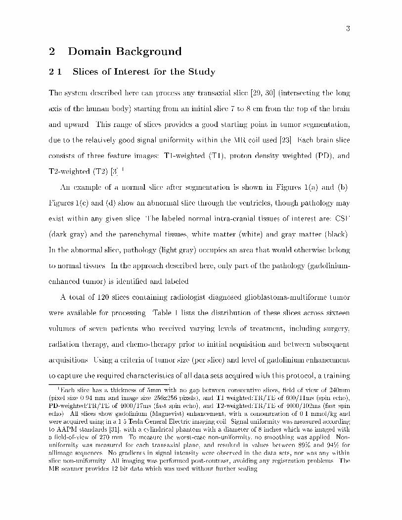
An example of a normal slice after segmentation is shown in Figures 1(a) and (b).

Figures 1(c) and (d) show an abnormal slice through the ventricles, though pathology may

exist within any given slice. The labeled normal intra-cranial tissues of interest are: CSF

(dark gray) and the parenchymal tissues, white matter (white) and gray matter (black).

In the abnormal slice, pathology (light gray) occupies an area that would otherwise belong

to normal tissues. In the approach described here, only part of the pathology (gadolinium-

enhanced tumor) is identi�ed and labeled.

A total of 120 slices containing radiologist diagnosed glioblastoma-multiforme tumor

were available for processing. Table 1 lists the distribution of these slices across sixteen

volumes of seven patients who received varying levels of treatment, including surgery,

radiation therapy, and chemo-therapy prior to initial acquisition and between subsequent

acquisitions. Using a criteria of tumor size (per slice) and level of gadolinium enhancement

to capture the required characteristics of all data sets acquired with this protocol, a training

1Each slice has a thickness of 5mm with no gap between consecutive slices, �eld of view of 240mm(pixel size 0.94 mm and image size 256x256 pixels), and T1-weighted:TR/TE of 600/11ms (spin echo),PD-weighted:TR/TE of 4000/17ms (fast spin echo), and T2-weighted:TR/TE of 4000/102ms (fast spinecho). All slices show gadolinium (Magnevist) enhancement, with a concentration of 0.1 mmol/kg andwere acquired using in a 1.5 Tesla General Electric imaging coil. Signal uniformity was measured accordingto AAPM standards [31], with a cylindrical phantom with a diameter of 8 inches which was imaged witha �eld-of-view of 270 mm. To measure the worst-case non-uniformity, no smoothing was applied. Non-uniformity was measured for each transaxial plane, and resulted in values between 89% and 94% forallimage sequences. No gradients in signal intensity were observed in the data sets, nor was any withinslice non-uniformity. All imaging was performed post-contrast, avoiding any registration problems. TheMR scanner provides 12-bit data which was used without further scaling.

4

(a)

Ventricles

(b)

(c)

Pathology

(d)

Figure 1: Slices of Interest: (a) raw data from a normal slice (T1-weighted, PD and T2-weighted images from left to right) (b) after segmentation (c) raw data from an abnormalslice (T1-weighted, PD and T2-weighted images from left to right) (d) after segmentation.White=white matter; Black=gray matter; Dark Gray=CSF; Light Gray=Pathology in (b)and (d).

subset of seventeen slices was created. The heuristics discussed in Section 3 were extracted

from the training subset through the process of \knowledge engineering." Knowledge

engineering is not automated, but human directed. Heuristics are expressed in general

terms, such as \higher end of the T1 spectrum" (which does not specify an actual T1

value). This provides knowledge that is more robust across slices, without regard to a

slice's particular thickness, scanning protocol, or signal intensity, as was the case in [23].

In contrast, multi-spectral e�orts such as [32] tune imaging parameters, which may limit

their application to slices with the same parameters. The generality of the system will be

discussed in Section 5.

2.2 Knowledge-Based Systems

Knowledge is any chunk of information that e�ectively discriminates one class type from

another [28]. In this case, tumor will have certain properties that other brain tissues will

5

Table 1: MR Slice Distribution. Parenthesis indicate the number of slices from that volumethat were used as training.

# Slices Extracted from Volume

Pat Baseline Repeat 1 Repeat 2 Repeat 3 Repeat 42 8 9(9) 9 - -4 6 7 7(2) - -5 6(6) - - - -1 9 10 10 9 83 9 9 - - -6 3 - - - -7 1 - - - -

not and visa-versa. In the domain of MRI volumes, there are two primary sources of

knowledge available. The �rst is pixel intensity in feature space, which describes tissue

characteristics within the MR imaging system, which are summarized in Table 2 (based

on a review of literature [33, 34, 35]). The second is image/anatomical space and includes

expected shapes and placements of certain tissues within the MR image, such as the

fact that CSF lies within the ventricles, as shown in Figure 1(a). Our previous e�orts

in [21, 22, 23] exploited both feature-domain and anatomical knowledge, using one source

to verify decisions based on the other source. The nature of tumors limits the use of

anatomical knowledge, since they can have any shape and occupy any area within the

brain. As a result, knowledge contained in feature space must be extracted and utilized

in a number of novel ways. As each processing stage is described in Section 3, the speci�c

knowledge extracted and its application will be detailed.

2.3 System Overview

A strength of the knowledge-based (KB) systems in [21, 22, 23] has been their \coarse-

to-�ne" operation. Instead of attempting to achieve their task in one step, incremental

re�nement is applied with easily identi�able tissues located and labeled �rst. Removing

labeled pixels from further consideration allows a \focus" to be placed on the remaining

6

Raw MR image data: T1, PD, and T2-weighted images.

Radiologist’s handlabeled ground truth tumor.

Tumor segmentation refined using ‘‘density screening.’’

STAGE THREE

Initial tumor segmentation using adaptive histogram thresholds on intracranial mask.

STAGE TWO

Intracranial mask created from initial segmentation.

STAGE ONE STAGE 0 Pathology Recognition.

Normal tissues are located and tested. Slices with abnormalities (such as in the white matter class shown) are segmented for tumor. Slices without abnormalities are not processed further.

Initial segmentationby unsupervisedclustering algorithm.

White matter class.

Removal of ‘‘spatial’’ regions that do not contain tumor. Remaining regions are labeledtumor and processing halts.

STAGE FOUR

Figure 2: System Overview.

7

Table 2: A Synopsis of T1, PD, and T2 E�ects on the Magnetic Resonance Image.TR=Repetition Time; TE=Echo Time.

Pulse Sequence E�ect Tissues(TR/TE) (Signal Intensity)

T1-weighted Short T1 relaxation Fat, Lipid-Containing Molecules,

(short/short) (bright) Proteinaceous Fluid, Paramagnetic

Substances (Gadolinium)

Long T1 relaxation Neoplasm, Edema, CSF,

(dark) Pure Fluid, In ammation

PD-weighted High proton density Fat, Fluids

(long/short) (bright)Low proton density Calcium, Air,

(dark) Fibrous Tissue, Cortical Bone

T2-weighted Short T2 relaxation Iron containing substances

(long/long) (dark) (blood-breakdown products)

Long T2 relaxation Neoplasm, Edema, CSF,

(bright) Pure Fluid, In ammation

(fewer) pixels, where more subtle trends may become clearer. The tumor segmentation

system is similarly designed. To better illustrate the system's organization, we present it

at a conceptual level. Figure 2 shows the primary steps in extracting tumor from raw MR

data. Section 3 described these steps in more detail.

The system has �ve primary steps. First a pre-processing stage developed in previous

works [21, 22, 23], called Stage Zero here, is used to detect deviations from expected

properties within the slice. Slices that are free of abnormalities are not processed further.

Otherwise, Stage One extracts the intra-cranial region from the rest of the MR image

based on information provided by pre-processing. This creates an image mask of the brain

that limits processing in Stage Two to only those pixels contained by the mask. In fact,

a particular Stage operates only on the foreground pixels that are contained in a mask

produced by the completion of the previous Stage.

An initial tumor segmentation is produced in Stage Two through a combination of

adaptive histogram thresholds in the T1 and PD feature images. The initial tumor seg-

mentation is passed on to Stage Three, where additional non-tumor pixels are removed via

8

a \density screening" operation. Density screening is based on the observation that pixels

of normal tissues are grouped more closely together in feature space than tumor pixels.

Stage Four completes tumor segmentation by analyzing each spatially disjoint \region"

in image space separately. Regions found to be free of tumor are removed, with those

regions remaining labeled as tumor. The resulting image is considered the �nal tumor

segmentation and can be compared with a ground truth image.

3 Classi�cation Stages

3.1 Stage Zero: Pathology Detection

All slices processed by the tumor segmentation system have been automatically classi�ed

as abnormal. They are known to contain glioblastoma-multiforme tumor based on ra-

diologist pathology reports. Since this work is an extension of previous work, knowledge

generated during \pre-processing" is available to the tumor segmentation system. Detailed

information can be found in [21, 22, 23], but a brief summary is provided.

Slice processing begins by using an unsupervised fuzzy c-means (FCM) clustering algo-

rithm [25, 26] to segment the slice. The initial FCM segmentation is passed to an expert

system which uses a combination of knowledge concerning cluster distribution in feature

space and anatomical information to classify the slice as normal or abnormal. Two ex-

amples of knowledge (implemented as rules) used in the predecessor system are: (1) in

a normal slice, CSF belongs to the cluster center with the highest T2 value in the intra-

cranial region; (2) in image space, all normal tissues are roughly symmetrical along the

vertical axis (de�ned by each tissue having approximately the same number of pixels in

each brain hemisphere), while tumors often have poor symmetry. Abnormal slices are

detected by their deviation from \expectations" concerning normal MR slices, such as the

one shown in Figure 2 whose white matter class failed to completely enclose the ventricle

area. An abnormal slice with the facts generated in labeling it abnormal are passed on to

the tumor segmentation system. Normal slices have all pixels labeled.

9

(a) (b) (c) (d) (e)

Figure 3: Building the Intra-Cranial Mask. (a) The original FCM-segmented image; (b)pathology captured in Group 1 clusters; (c) intra-cranial mask using only Group 2 clusters;(d) mask after including Group 1 clusters with tumor; (e) mask after extra-cranial regionsare removed.

(a) (b) (c)

Figure 4: (a) Initial segmented image; (b) a quadrangle overlaid on (a); (c) classes thatpassed quadrangle test.

3.2 Stage One: Building the Intra-Cranial Mask

The �rst step in the system presented here is to isolate the intra-cranial region from the

rest of the image. During pre-processing, extra and intra-cranial pixels were distinguished

primarily by separating the clusters from the initial FCM segmentation into two groups:

Group 2 for brain tissue clusters, and Group 1 for the remaining extra-cranial clusters.

Occasionally, enhancing tumor pixels can be placed into one or more Group 1 clusters

with high T1-weighted centroids. In most cases, these pixels can be reclaimed through a

series of morphological operations (described below). As shown in Figures 3(b) and (c),

however, the tumor loss may be too severe to recover morphologically without distorting

the intra-cranial mask.

10

Group 1 clusters with signi�cant \Lost Tumor" can be located, however. During pre-

processing, Group 1 and 2 clusters were separated based on the observation that extra-

cranial tissues surround the brain and are not found within the brain itself. A \quadrangle"

was developed by Li in [21, 36] to roughly approximate the intra-cranial region. Group

1 and 2 clusters were then discriminated by counting the number of pixels a cluster had

within the quadrangle. Clusters consisting of extra-cranial tissues will have very few pixels

inside this estimated brain, while clusters of intra-cranial tissues will have a signi�cant

number. An example is shown in Figure 4.

A Group 1 cluster is considered to have \Lost Tumor" here if more than 1% of its

pixels were contained in the approximated intra-cranial region. The value of 1% is used

to maximize the recovery of lost tumor pixels because extra-cranial clusters with no lost

tumor will have very few pixels within the quadrangle, if any at all. Pixels belonging

to Lost Tumor clusters (Figure 3(b)) are merged with pixels from all Group 2 clusters

(Figure 3(c)) and set to foreground (a non-zero value), with all other pixels in the image

set to background (value=0). This produces a new intra-cranial mask similar to the one

shown in Figure 3(d).

Since a Lost Tumor cluster is primarily extra-cranial, its inclusion in the intra-cranial

mask introduces areas of extra-cranial tissues, such as the eyes and skin/fat/muscle. To

remove these unwanted extra-cranial regions (and recover smaller areas of lost tumor,

mentioned above), a series of morphological operations [37] are applied, which use window

sizes that are the smallest possible (to minimize mask distortion) while still producing the

desired result.

Small regions of extra-cranial pixels are removed and separation of the brain from

meningial tissues is enhanced by applying a 5�5 closing operation to the background. Then

the brain is extracted by applying an eight-wise connected components operation [37] and

keeping only the largest foreground component (the intra-cranial mask). Finally, \gaps"

along the periphery of the intra-cranial mask are �lled by �rst applying a 15� 15 closing,

11

then a 3� 3 erosion operation. An example of the �nal intra-cranial mask can be seen in

Figure 3(e).

3.3 Stage Two: Multi-spectral Histogram Thresholding

Given an intra-cranial mask from Stage One, there are three primary tissue types: pathol-

ogy (which can include gadolinium-enhanced tumor, edema, and necrosis), the brain

parenchyma (white and gray matter), and CSF. We would like to remove as many pixels

belonging to normal tissues as possible from the mask.

Each MR voxel of interest has a hT1; PD; T2i location in <3, forming a feature-space

distribution. Based on the knowledge in Table 2, and the fact that pixels belonging to

the same tissue type will exhibit similar relaxation behaviors (T1 and T2) and water con-

tent (PD), they will then also have approximately the same location in feature space [38].

Figure 5(a) shows the signal-intensity images of a typical slice, while (b) and (c) show

histogram for the bivariate features T1/PD and T2/PD, respectively, with approximate

tissue labels overlaid. There is some overlap between classes because the graphs are pro-

jections and also due to \partial-averaging" where di�erent tissue types are quantized into

the same voxel.

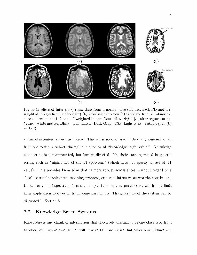
The typical relationships between enhancing tumor and other brain tissues can also

be seen in Figure 6, which are histograms for each of the three feature images. These

distributions were examined and interviews were conducted with experts concerning the

general makeup of tumorous tissue, and the behavior of gadolinium enhancement in the

three MRI protocols. From these sources, a set of heuristics were extracted that could be

included in the system's knowledge base:

1. Gadolinium-enhanced tumor pixels occupy the higher end of the T1 spectrum.

2. Gadolinium-enhanced tumor pixels occupy the higher end of the PD spectrum,

though not with the degree of separation found in T1 space [39].

12

(a)

T1-Weighted Value

PD

-Wei

gh

ted

Val

ue

CPa

Pa

Pa

T

T

T

High PD

High T1

(b)

PD-Weighted Value

T2-

Wei

gh

ted

Val

ue C

PaPa

Pa

T

T

High T2

High PD

(c)

Figure 5: (a) Raw T1, PD, and T2-weighted Data. The distribution of intra-cranial pixelsare shown in (b) T1-PD and (c) PD-T2 feature space. C = CSF, Pa = ParenchymalTissues, T = Tumor

3. Gadolinium-enhanced tumor pixels were generally found in the \middle" of the T2

spectrum, making segmentation based on T2 values di�cult.

4. Slices with greater enhancement had better separation between tumor and non-tumor

pixels, while less enhancement resulted in more overlap between tissue types.

Analysis of these heuristics revealed that histogram thresholding could provide a sim-

ple, yet e�ective, mechanism for gross separation of tumor from non-tumor pixels (and

thereby an implementation for the heuristics). In fact, in the T1 and PD spectrums, the

signal intensity having the greatest number of pixels, that is, the histogram \peaks," were

found to be e�ective thresholds that work across slices, even those with varying degrees of

13

(a) Raw Data

T1-Weighted Value High T1Low T1

Pix

el C

ou

nt

Intracranial Pixels

"Ground Truth" Tumor

(b) T1-weighted Histogram

PD-Weighted Value High PDLow PD

Pix

el C

ou

nt

Intracranial Pixels

"Ground Truth" Tumor

(c) PD-weighted Histogram

T2-Weighted Value High T2Low T2

Pix

el C

ount

Intracranial Pixels

"Ground Truth" Tumor

(d) T2-Weighted Histogram

Figure 6: Histograms for Tumor and the Intra-Cranial Region. Solid black lines indicatesthresholds in T1 and PD-weighted space.

14

(a) (b) (c) (d)

Figure 7: Multi-spectral Histogram Thresholding of Figure 6. (a) T1-weighted threshold-ing; (b) PD-weighted thresholding; (c) Intersection of (a) and (b); (d) Ground truth.

gadolinium enhancement. An example of this is shown in Figure 6. The T2 image had no

such property that was consistent across all training slices and was excluded.

For a pixel to survive thresholding, its signal intensity value in a particular feature

had to be greater than the intensity threshold for that feature. Figures 7(a) and (b) show

the results of applying the T1 and PD histogram \peak" thresholds in Figures 6(b) and

(c). In both of these thresholded images a signi�cant number of non-tumor pixels have

been removed, but some non-tumor pixels remain in each thresholded image. Since the

heuristics listed above state that gadolinium enhanced tumor has a high signal intensity in

both the T1 and PD features, additional non-tumor pixels can be removed by intersecting

the two images (where a pixel remains only if it's present in both images). An example is

shown in Figure 7(c).

3.4 Stage Three: \Density Screening" in Feature Space

The thresholding process in Stage Two provides a good initial tumor segmentation, such

as the one shown in Figure 7(c). Comparing it with the ground truth image Figure 7(d),

a number of pixels in the initial tumor segmentation are not found in the ground truth

image and should be removed. Additional thresholding is di�cult to perform, however,

without possibly removing tumor as well as non-tumor pixels.

15

Low PD

HighPDLow

T1 High T1

Nu

mb

er

of

Pix

els

Low

High

(a) 2D-Histogram Projection

Lo

w P

D

Low T1 High T1

Hig

h P

D

(b) ScatterplotBefore Screening

Low T1 High T1

Lo

w P

DH

igh

PD

(c) ScatterplotAfter Screening

(d) Initial Tumor (e) Removed Pixels (Black) (f) Ground Truth

Figure 8: Density Screening Initial Tumor Segmentation From Figure 7(c).

Pixels belonging to the same tissue type will have similar signal intensities in the

three feature spectrums. Because normal tissue types have a more or less uniform cellular

makeup [33, 34, 35], their distribution in feature space will be relatively concentrated [38].

In contrast, tumor can have signi�cant variance, depending on the local degrees of enhance-

ment and tissue inhomogeneity within the tumor due to the presence of edema, necrosis,

and possibly some parenchymal cells captured by the partial-volume e�ect. Figures 5 (b)

and (c) show the di�erent spreads in feature space for normal and tumor pixels. Pixels

belonging to parenchymal tissues and CSF are grouped more densely by intensity, while

pixels belonging to tumor are more widely distributed.

By exploiting this \density" property, non-tumor pixels can be removed without a�ect-

ing the presence of tumor pixels. Called \density screening," the process begins by creating

16

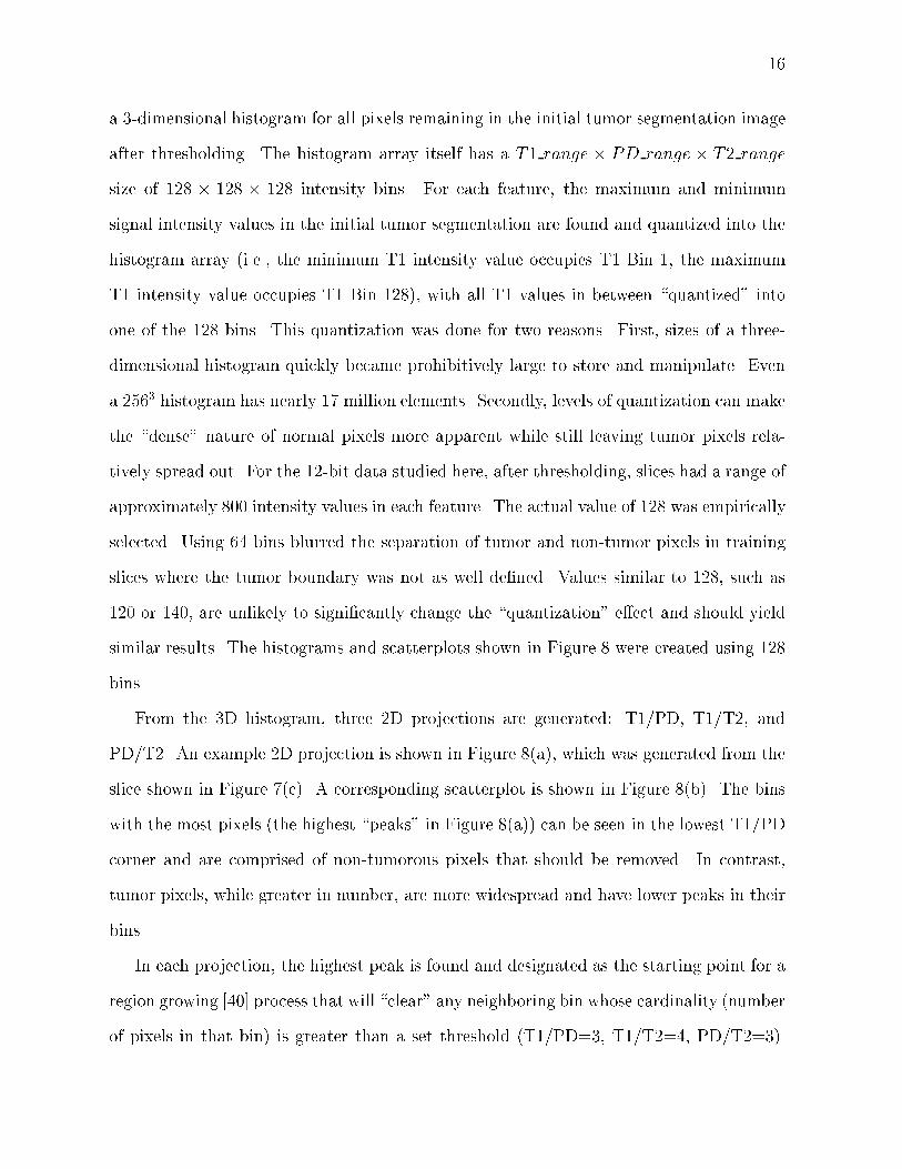
a 3-dimensional histogram for all pixels remaining in the initial tumor segmentation image

after thresholding. The histogram array itself has a T1 range � PD range � T2 range

size of 128 � 128 � 128 intensity bins. For each feature, the maximum and minimum

signal intensity values in the initial tumor segmentation are found and quantized into the

histogram array (i.e., the minimum T1 intensity value occupies T1 Bin 1, the maximum

T1 intensity value occupies T1 Bin 128), with all T1 values in between \quantized" into

one of the 128 bins. This quantization was done for two reasons. First, sizes of a three-

dimensional histogram quickly became prohibitively large to store and manipulate. Even

a 2563 histogram has nearly 17 million elements. Secondly, levels of quantization can make

the \dense" nature of normal pixels more apparent while still leaving tumor pixels rela-

tively spread out. For the 12-bit data studied here, after thresholding, slices had a range of

approximately 800 intensity values in each feature. The actual value of 128 was empirically

selected. Using 64 bins blurred the separation of tumor and non-tumor pixels in training

slices where the tumor boundary was not as well de�ned. Values similar to 128, such as

120 or 140, are unlikely to signi�cantly change the \quantization" e�ect and should yield

similar results. The histograms and scatterplots shown in Figure 8 were created using 128

bins.

From the 3D histogram, three 2D projections are generated: T1/PD, T1/T2, and

PD/T2. An example 2D projection is shown in Figure 8(a), which was generated from the

slice shown in Figure 7(c). A corresponding scatterplot is shown in Figure 8(b). The bins

with the most pixels (the highest \peaks" in Figure 8(a)) can be seen in the lowest T1/PD

corner and are comprised of non-tumorous pixels that should be removed. In contrast,

tumor pixels, while greater in number, are more widespread and have lower peaks in their

bins.

In each projection, the highest peak is found and designated as the starting point for a

region growing [40] process that will \clear" any neighboring bin whose cardinality (number

of pixels in that bin) is greater than a set threshold (T1/PD=3, T1/T2=4, PD/T2=3).

17

This will result in a new scatterplot similar to that shown in Figure 8(c). A pixel is removed

from the tumor segmentation if it corresponds to a bin that has been \cleared" in any of

the three feature-domain projections. Figures 8(d) and (e) are the tumor segmentation

before and after the entire density screening process is completed. Note that the resulting

image is closer to ground truth.

The thresholds used were determined from training slices by creating a 3D histogram,

including 2D projections, using only pixels contained in the initial tumor segmentation.

Then the ground truth tumor pixels for each slice were overlaid on the respective projec-

tions. So, given a 3D histogram of an initial tumor segmentation, all pixels not in the

ground truth image are removed, leaving only tumor behind without changing the dimen-

sions and quantization levels of the histogram. The respective 2D projections of all training

slices were examined. It was found that the smallest bin cardinality bordering a bin occu-

pied by known non-tumor pixels made an accurate threshold for the given projection. It

should be noted, however, that the thresholds were based on the 256� 256 images used in

this research and would need to be scaled to accommodate images of di�erent sizes, such

as 512� 512.

3.5 Stage Four: Region Analysis and Labeling

In Stages Two and Three, the knowledge extracted up to this point was applied to pixels

individually. Stage Four, allows spatial information to be introduced by considering pixels

on a region or component level.

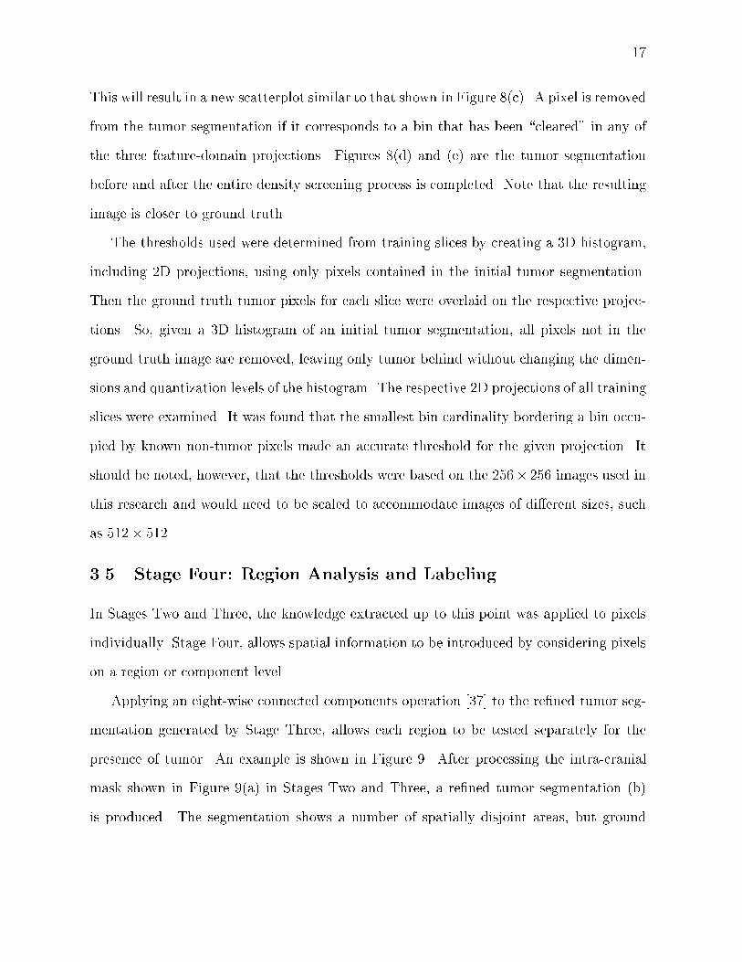
Applying an eight-wise connected components operation [37] to the re�ned tumor seg-

mentation generated by Stage Three, allows each region to be tested separately for the

presence of tumor. An example is shown in Figure 9. After processing the intra-cranial

mask shown in Figure 9(a) in Stages Two and Three, a re�ned tumor segmentation (b)

is produced. The segmentation shows a number of spatially disjoint areas, but ground

18

(a) (b) (c)

Figure 9: Regions in Image Space. After processing the intra-cranial mask (a), (b) is aninitial tumor segmentation. Only one region, as shown in the ground-truth image (c) isactual tumor. Region analysis discriminates between tumorous and non-tumorous regions.

truth tumor in Figure 9(c) shows that only one region actually contains tumor. Therefore,

decisions must be made regarding which regions contain tumor and which do not.

3.5.1 Removing Meningial Regions

In addition to tumor, meningial tissues immediately surrounding the brain, such as the

dura or pia mater, receive gadolinium infused blood. As a result they can have a high T1

signal intensity that may interfere with the knowledge base's assumption in Section 3.5.2

that regions with the highest T1 value are most likely tumor. These extra-cranial tissues

can be identi�ed and removed via anatomical knowledge by noting that since they are thin

membranes, meningial regions should lie along the periphery of the brain in a relatively

narrow margin.

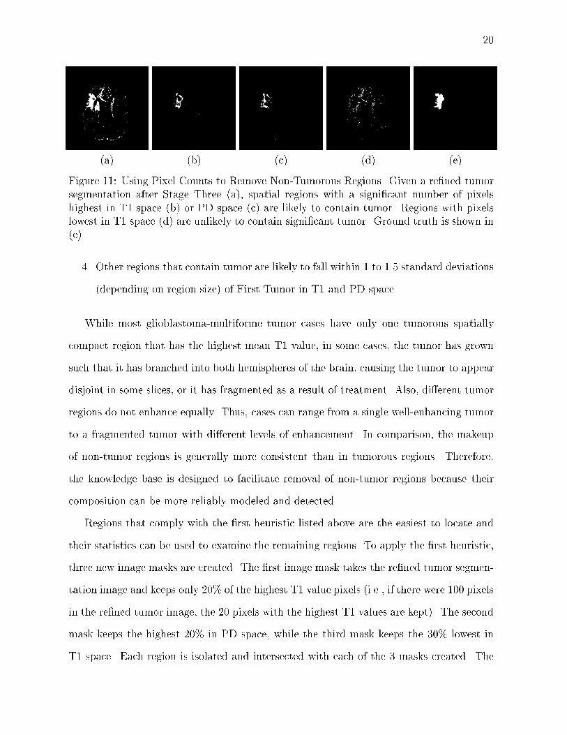
Figure 10 shows that an approximation of the brain periphery can be used to detect

meningial tissues. The unusual shape of the intra-cranial region is due to prior resection

surgery. The periphery is created by applying a 7�7 erosion operation to the intra-cranial

mask and subtracting the resultant image from the original mask, as shown in Figure 10(a-

c). Each component or separate region in the re�ned tumor mask is now intersected with

the brain periphery. Any region which has more than 50% of its pixels contained in

the periphery is marked as meningial tissue and removed. Figure 10(d) shows a tumor

segmentation which is intersected with the periphery from Figure 10(c). In Figure 10(e),

19

(a) (b) (c) (d) (e)

Figure 10: Removing Meningial Pixels. A \ring" that approximates the brain peripheryis created by applying a 7 � 7 erosion operation to the intra-cranial mask (a), resultingin image (b). Subtracting (b) from (a), creates a \ring", shown in (c). By overlayingthis \ring" onto a tumor segmentation (d), small regions of meningial tissues (e) canbe detected and removed. The unusual shape of the intra-cranial region is due to priorresection surgery.

the pixels that will be removed by this operation are shown and they are indeed meningial

pixels.

3.5.2 Removing Non-Tumor Regions

Once any extra-cranial regions have been removed, the knowledge base is applied to dis-

criminate between regions with and without tumor based on statistical information about

the region. A region mean, standard deviation, and skewness in hT1i, hPDi, and hT2i

feature space respectively are used as features. The concept exploited is that trends and

characteristics described at a pixel level in Table 2 and Section 3.3 are also applicable on a

region level. By sorting regions in feature space based upon their mean values, rules based

on their relative order can be created:

1. Large regions that contain tumor will likely contain a signi�cant number of pixels

that are of highest intensity in T1 and PD space, while regions without tumor likely

contain a signi�cant number of pixels of lowest intensity in T1 and PD space.

2. The means of regions with similar tissue types neighbor one another in feature space.

3. The intra-cranial region with the highest mean T1 value and a \high" PD and T2

value, is considered \First Tumor," against which all other regions are compared.

20

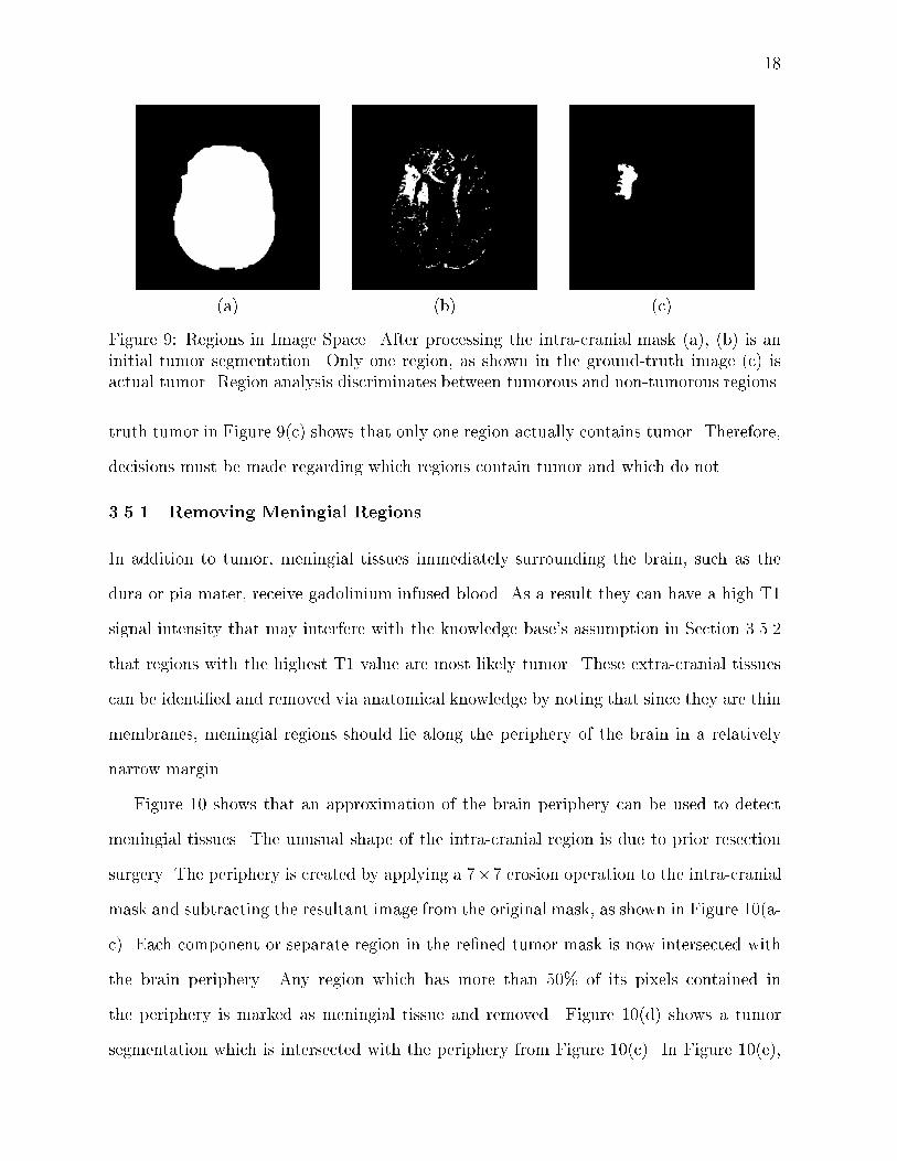
(a) (b) (c) (d) (e)

Figure 11: Using Pixel Counts to Remove Non-Tumorous Regions. Given a re�ned tumorsegmentation after Stage Three (a), spatial regions with a signi�cant number of pixelshighest in T1 space (b) or PD space (c) are likely to contain tumor. Regions with pixelslowest in T1 space (d) are unlikely to contain signi�cant tumor. Ground truth is shown in(e).

4. Other regions that contain tumor are likely to fall within 1 to 1.5 standard deviations

(depending on region size) of First Tumor in T1 and PD space.

While most glioblastoma-multiforme tumor cases have only one tumorous spatially

compact region that has the highest mean T1 value, in some cases, the tumor has grown

such that it has branched into both hemispheres of the brain, causing the tumor to appear

disjoint in some slices, or it has fragmented as a result of treatment. Also, di�erent tumor

regions do not enhance equally. Thus, cases can range from a single well-enhancing tumor

to a fragmented tumor with di�erent levels of enhancement. In comparison, the makeup

of non-tumor regions is generally more consistent than in tumorous regions. Therefore,

the knowledge base is designed to facilitate removal of non-tumor regions because their

composition can be more reliably modeled and detected.

Regions that comply with the �rst heuristic listed above are the easiest to locate and

their statistics can be used to examine the remaining regions. To apply the �rst heuristic,

three new image masks are created. The �rst image mask takes the re�ned tumor segmen-

tation image and keeps only 20% of the highest T1 value pixels (i.e., if there were 100 pixels

in the re�ned tumor image, the 20 pixels with the highest T1 values are kept). The second

mask keeps the highest 20% in PD space, while the third mask keeps the 30% lowest in

T1 space. Each region is isolated and intersected with each of the 3 masks created. The

21

Table 3: Region Labeling Rules Based on Pixel Presence.Region Size Pixels in intersections with the 3 masks Action

� 5 Any Bottom T1 Pixels AND RemoveLess than 2 Top T1 Pixels Non-Tumor

� 500 More than RegionSize � 0:06 Top T1 Pixels Label AsTumor

� 5 No Top T1 Pixels AND RemoveMore Than RegionSize � 0:005 Bottom T1 Pixels AND

Less Than RegionSize� 0:01 Top PD Pixels

number of pixels of the region in a particular mask is recorded and compared with the

rules listed in Table 3. An example is shown in Figure 11.

Regions that do not activate any of the rules in Table 3 remain unlabeled and are

analyzed using the last two heuristics.

According to the third heuristic, given a region that has been positively labeled tumor

as a point of reference, a search can be made in feature space for neighboring tumor

regions. Normally, the region with the highest T1 mean value can be selected as this point

of reference (called \First Tumor"). To guard against the possibility that an extra-cranial

region (usually meningial tissues at the inter-hemispheric �ssure) has been selected instead,

the selected region is veri�ed via the heuristic that a tumor region will not only have a very

high T1 mean value, but will also occupy the highest half of all regions in sorted PD and

T2 mean space. For example, if there were 10 regions total, the region being tested must

be one of the 5 highest mean values in both PD and T2 space. If the candidate region

passes, it is con�rmed as First Tumor. Otherwise, it is discarded and the region with the

next highest T1 mean value is selected for testing as First Tumor.

Once First Tumor has been con�rmed, the search for neighboring tumor regions can

begin. Although tumorous regions can have between-slice variance, the third and fourth

heuristics hold for the purpose of separating tumor from non-tumor regions within a given

slice. Furthermore, the standard deviations in T1 and PD space of a known tumor region

were found to be a useful and exible distance measure.

22

Table 4: Region Labeling Rules Based on Statistical Measurements. Largest is the largestknown tumor region.

(a) Rules Based on Standard Deviation (SD) of \First Tumor"Region Size If Region's Mean Values are: Action

� 10 OR More than 1 SD away in T1 space OR Remove� Largest=4 More than 1 SD away in PD space.

� 10 AND More than 1.5 SD away in T1 space AND Remove� Largest=4 More than 1.5 SD away in PD space.

(b) Labeling Rules Based on Region Statistics� 100 Region T1 Skewness � 0:75 AND Remove

Region PD Skewness � 0:75 AND

Region T2 Skewness � 0:75

Table 4(a) lists the two rules that used the standard deviation to remove non-tumor

regions, based on the size (number of pixels) of the region being tested. The rule in

Table 4(b) serves as a tie-breaker for some regions that were not labeled before. The term

Largest is used to indicate the largest known tumor region. In most cases there was only

a single tumor region, so the \�rst tumor" region was also the Largest region. In cases

where tumor was fragmented, however, a larger tumorous region will provide a more robust

mean and standard deviation for the distance measure. Therefore, the system would �nd

Largest by searching for the largest region that was within one standard deviation in both

T1 and PD space to the First Tumor region.

After the rules in Table 4 are applied, all regions that were not removed are labeled as

tumor, and the segmentation process terminates.

4 Results

4.1 Knowledge-Based Vs. Ground Truth

A total of 120 slices, including the 17 training slices described in Section 2.1, were within

the slice range of the system and known to contain tumor. After processing by the system,

the slices were compared with \ground-truth" tumor segmentations that were created by

radiologist hand labeling [41]. Error was found between the two segmentations, both false

23

Table 5: Comparison of Knowledge-Based Tumor Segmentation Vs. Hand Labeled Seg-mentation Per Volume.

Patient Scan True False False Tumor Percent Corr. \True" FalsePositive Positive Negative Size Match Ratio Positive

1 Base 6921 2700 234 7155 0.97 0.78 801 R1 7038 3879 196 7234 0.97 0.70 4671 R2 7285 4869 176 7461 0.98 0.65 4961 R3 6206 3261 166 6372 0.97 0.72 2271 R4 5930 3130 48 5978 0.99 0.63 472 Base 7892 5976 408 8300 0.95 0.54 182 R1 10092 3481 1059 11151 0.91 0.75 662 R2 14822 4961 1012 15834 0.94 0.78 2193 Base 8917 1635 581 9498 0.94 0.85 473 R1 5003 2619 169 5172 0.97 0.71 894 Base 3054 1536 75 3129 0.98 0.73 1244 R1 3627 2082 659 4286 0.85 0.43 10924 R2 2506 1020 1103 3609 0.69 0.46 4955 Base 829 573 173 1002 0.83 0.54 1616 Base 1425 624 0 1425 0.96 0.78 537 Base 177 175 0 177 1.00 0.51 54

positives (where the system indicated tumorous pixels where ground truth did not) and

false negatives (where ground truth indicated tumorous pixels that the system did not).

To compare how well (on a pixel level) the KB method corresponded with ground truth,

two measures were used. The �rst, \percent match," is simply the number of true positives

divided by the total tumor size. The second, is called a \correspondence ratio," and was

created to account for the presence of false positives:

Correspondence Ratio =True Pos.� (0:5 � False Pos.)

Number Pixels in Ground Truth Tumor

For comparing on a per volume basis, the average value for Percent Match was generated

using:

Average % Match =

Pslices in seti=1

(% match)i� (number ground truth pixels)

i

Pslices in seti=1

(number ground truth pixels)i

The average value for the Correspondence Ratio is similarly generated.

24

Table 5 lists the results of the KB system on a per-volume basis. The results show

that the KB system performs well overall. We note that 89 of the 120 slices had a Percent

Match rating of 90% or higher. Slices that showed signi�cant False Negative presence

were primarily the result of two situations. Some tumor could be lost during the intra-

cranial extraction stage. One test slice (from Patient 4 Repeat Scan 2) had signi�cant

tumor pixels lost during the morphological operations following tumor recovery from the

quadrangle test. In four uppermost test slices (all from Patient 1), part of the tumor

had grown beyond the intra-cranial region into an area normally occupied by surrounding

meningial membranes, which have an increased percentage presence in the uppermost

slices. The tumor's location within these membranes, combined with the reduced brain

size complicated extraction. Other instances of tumor loss occurred when the system

captured the tumor borders, but not its interior, possibly due to more subtle gadolinium

enhancement (still detected by the radiologist, but not clear enough in feature space) [42],

or cases where necrosis prevented circulation of the enhancing agent, but the radiologist

made a conservative diagnosis and marked the area as tumor.

Overall, the KB approach tended to signi�cantly overestimate the tumor volume. Only

one volume in Table 5 shows underestimation (Patient 4 Repeat Scan 2), and that can

be traced to one test slice with signi�cant tumor underestimation (described above). The

tendency to over-estimate is consistent with the system's paradigm, since only those pixels

positively believed to be non-tumor are removed, defaulting areas of uncertainty to be

labeled as tumor.

To show the nature of the false positives in the knowledge-based system, an additional

measurement, \true" false positives, were added to Table 5 to indicate how many of the

false positives were actually not connected spatially to any ground truth tumor. This

number is less than 15% of the false positives with 2 exceptions. An examination of the

process of creating ground-truth images revealed a 5% inter-observer variability in tumor

volume [41]. We also note that all brain tumors have micro-in�ltration beyond the borders

25

Table 6: Comparison of kNN (k=7) Tumor Segmentation Vs. Hand Labeled SegmentationPer Volume.

Patient Scan True False False Percent Corr.Positive Negative Positive Match Ratio

1 Base 6430 782 3592 0.89 0.641 R1 6548 781 5410 0.89 0.521 R2 6544 925 5032 0.88 0.541 R3 5643 751 5227 0.88 0.471 R4 5274 935 5500 0.85 0.412 Base 6227 2167 3287 0.74 0.552 R1 5933 5217 6840 0.53 0.232 R2 7905 8199 7498 0.49 0.263 Base 6972 2570 4027 0.73 0.523 R1 3695 1476 2903 0.71 0.434 Base 2191 938 1716 0.70 0.434 R1 2105 2193 3432 0.49 0.094 R2 1988 1614 2869 0.55 0.155 Base 874 144 1490 0.86 0.136 Base 319 116 1085 0.22 -0.167 Base 175 1 1128 0.99 -2.21

de�ned with gadolinium enhancement. This is especially true in glioblastoma-multiformes,

which are the most aggressive grade of primary glioma brain tumors, and no one can tell

the exact tumor borders without invasive histopathological methods [24, 42, 43] and these

were unavailable. As a result, ground truth images mark the areas of tumor exhibiting

the most angiogenesis (formation of blood vessels, resulting in the greatest gadolinium

concentration). Therefore, the knowledge-based system may capture tumor boundaries

that extend into areas showing lower degrees of angiogenesis (which would still be treated

during therapy) [43].

4.2 Knowledge-Based Vs. kNN

One of the advantages of this KB approach is that human based training regions of interest

(ROI's), currently required for supervised techniques [44], are not necessary after rule

acquisition. Yet, results can be as good, if not better, than those obtained from supervised

methods, without the need to for time-consuming ROI selection, which make such methods

26

impractical for clinical use and do not guarantee satisfactory performance. Table 6 shows

how well the supervised k-nearest neighbors (kNN) algorithm (k=7) [45] performed on

the same slices processed by the KB system. The kNN method �nds the k=7 labeled

pixels from the ROI's closest to a test pixel and classi�es the test pixel into the majority

class of the associated ROI's. The kNN algorithm has been shown to be less sensitive

to ROI selection than seed-growing, a commercially available supervised approach (ISG

Technologies, Toronto, Canada) [44, 46].

It must be noted that the kNN results include extra-cranial pixels in the tumor class

because kNN is applied to the whole image. No extraction of the actual tumor is done,

which would require additional supervisor intervention. The kNN numbers shown here

were the mean results over multiple trials of ROI selection, meaning that all kNN slice

segmentations were e�ectively training slices. Furthermore, kNN introduces the question

of inter and intra-observer variability, which was rated at approximately 9% and 5% re-

spectively [47]. In contrast, the KB system was built from a small subset of the available

slices and processed 103 slices in unsupervised mode with a static rule set allowing for

complete repeatability.

4.3 Evaluation Over Repeat Scans

Examining tumor growth/shrinkage over multiple acquisitions, the total tumor volume for

ground truth, the KB method, and kNN are compared in Table 7 and Figure 12. The

kNN volumes shown are means over one or more trials and include the total inter and

intra-observer standard deviation. The KB system is closer to the ground truth volume

in 8 of the 16 cases, though the di�erence between the KB and kNN methods was less

than the kNN standard deviation in 7 of the cases. More importantly, comparing their

respective performances in Tables 5 and 6, the KB method has a smaller number of false

negatives than the kNN method in all volumes compared, suggesting the KB method more

closely matched ground truth than kNN.

27

Table 7: Tumor Volume Comparison (Pat. = Patient, GT = Ground Truth Volume, KB= Knowledge Based, kNN SD = kNN Standard Deviation, kNN Trial = Number of Trials,kNN Obs. = Number of kNN Observers.)

Pat. Scan GT KB kNN kNN kNN kNNVolume Volume Volume SD Trials Obs.

1 Base 7155 9621 10022 732 5 21 R1 7234 10917 11958 2236 5 21 R2 7461 12154 11576 1615 5 21 R3 6372 9467 10870 4395 5 21 R4 5978 9060 10774 891 5 22 Base 8300 13868 9514 1635 5 22 R1 11151 13573 12773 2375 5 22 R2 15834 19783 15403 1942 5 23 Base 9498 10552 10999 1323 5 33 R1 5172 7622 6598 1830 5 34 Base 3129 4590 3907 643 4 24 R1 4286 5709 5537 592 4 24 R2 3609 3526 4857 727 4 25 Base 1002 1042 2364 N/A 1 16 Base 1425 2049 1404 N/A 1 17 Base 177 352 1303 207 4 2

Both methods showed an instance where the ground truth volume grew, yet they re-

ported tumor shrinkage. The kNN method failed to correctly predict tumor growth in

Patient 1, from Repeat Scan 1 to 2. Since the kNN volumes are based on multiple trials,

it is di�cult to assign a speci�c cause. The KB method failed to predict tumor growth

in Patient 2, from the Baseline scan to Repeat Scan 1. According to pathology reports,

the Baseline scan contained a signi�cant amount of uid, possibly hemmorage, which ar-

ti�cially brightened regions surrounding the tumor in the PD scan and made the border

between non-tumor and tumor pixels unusually di�use. This distorted the histogram from

which the initial tumor segmentation was based, resulting in signi�cant overestimation

of tumor volume. In Repeat Scan 1, however, not only had the uid disappeared, but

pathology reports noted a slight decrease in gadolinium enhancement. Thus, the initial

28

Tu

mo

r V

olu

me

(vo

xels

)

Scanning Session

Knowledge Based Versus Hand Labeling

GT

KB

KNN

13000

0 1 2 3 45000

6000

7000

8000

9000

10000

11000

12000

(a) Patient 1

Tu

mo

r V

olu

me

(vo

xels

)

Scanning Session

Knowledge Based Versus Hand Labeling

GT

KNN

KB

8000

10000

12000

14000

16000

18000

20000

0 1 2

(b) Patient 2

0 1

Tu

mo

r V

olu

me

(vo

xels

)

Scanning Session

Knowledge Based Versus Hand Labeling

KB

KNN

GT

5000

6000

7000

8000

9000

10000

11000

(c) Patient 3

0 1 2

Tu

mo

r V

olu

me

(vo

xels

)

Scanning Session

Knowledge Based Versus Hand Labeling

GT

KNN

KB

3000

3500

4000

4500

5000

5500

6000

(d) Patient 4

Figure 12: Tracking Tumor Growth/Shrinkage Over Repeat Scans. KB=Knowledge-BasedSystem. kNN=k-Nearest Neighbors. GT=Ground Truth.

overestimation followed by the decreased gadolinium enhancement caused the trend to ap-

pear to be tumor shrinkage instead of growth. Patient 2 had received signi�cant treatment

(surgery and radiation therapy) prior to scanning, making the tumor boundaries particu-

larly di�cult to detect. In fact, a review of the pathology reports showed that radiologist

estimations of the tumor volume had to be revised.

Finally, Figure 13 shows examples of the KB system's correspondence to hand-labeled

tumor in slices. Figures 13(a-c) show a worst case segmentation, while (d-f) and (g-i) show

an average and best case segmentation respectively. All three examples are from the test

29

(a) Raw Image (b) KB Tumor (c) GT Tumor

(d) Raw Image (e) KB Tumor (f) GT Tumor

(g) Raw Image (h) KB Tumor (i) GT Tumor

Figure 13: Comparison of Knowledge-Based Tumor Segmentation Vs. Ground Truth.Worst case (a-c), average case (d-f), and best case (g-i).

set.

5 Discussion

We have described a knowledge-based multi-spectral analysis tool that segments and labels

glioblastoma-multiforme tumor. The guidance of the knowledge base gives this system

additional power and exibility by allowing unsupervised segmentation and classi�cation

decisions to be made through iterative/successive re�nement. This is in contrast to most

other multi-spectral e�orts such as [8, 10, 12] which attempt to segment the entire brain

image in one step, based on either statistical or (un)supervised classi�cation methods.

30

The knowledge base was initially built with a general set of heuristics comparing the

e�ects of di�erent pulse sequences on di�erent types of tissues, as shown in Table 2. This

process is called \knowledge-engineering" as we had to decide which knowledge was most

useful for the goal of tumor segmentation, followed by the process of implementing such

information into a rule-based system. More importantly, the training set used was quite

small - seventeen slices over three patients. Yet, the system performed well. A larger

training set would most likely allow new and more e�ective trends and characteristics to

be revealed. Thresholds used to handle a certain subset of the training set could be better

generalized.

The slices processed had a relatively large thickness of 5mm. Thinner slices which

exhibit a reduced partial-volume e�ect and allow better tissue contrast. While relying

on feature space distributions, the system was developed using general tissue character-

istics, such as those listed in Table 2, and relative relationships between tissues to avoid

dependence upon speci�c feature-domain values. The particular slices were acquired with

the same parameters, but gadolinium-enhancement has been found to be generally very

robust in di�erent protocols and thickness [48, 39]. Should acquisition parameter depen-

dence become an issue, given a large enough training base across multiple parameters,

the knowledge base could automatically adjust to a slice's speci�c parameters since such

information is easily included when processing starts. The patient volumes processed had

received various degrees of treatment, including surgery, radiation and chemo-therapy both

before and between scans. Yet, despite the changes these treatments can cause, such as

demyelinization of white matter, no modi�cations to the knowledge based system were

necessary. Other approaches, like neural networks [49] or any sort of supervised method

which is based on a speci�c set of training examples could have di�culties in dealing with

slightly di�erent imaging protocols and the e�ects of treatment.

As stated in the introduction, no method of quantitating tumor volumes is widely ac-

cepted and used in clinical practice [4]. A method by the Eastern Cooperative Oncology

31

group [5] approximates tumor area in the single MR slice with the largest contiguous,

well-de�ned tumor evident. The longest tumor diameter is multiplied by its perpendicular

to yield an area. Changes greater than 25% in the area of a tumor over time are used, in

conjunction with visual observations, to classify tumor response to treatment into �ve cat-

egories from complete response (no measurable tumor left) to progression. This approach

does not address full tumor volume, depends on the exact boundary choices, and the

shape of the tumor [2, 5]. By itself, the approach can lead to inaccurate growth/shrinkage

decisions [6].

The promise of the knowledge-based system as a useful tool is demonstrated by the

successful performance of the system on the processed slices. The �nal KB segmentations

compare well with radiologist-labeled \ground truth" images. The knowledge-based sys-

tem also compared well with supervised kNN method, and was able to segment tumor

without the need for (multiple) human-based ROI's or post-processing, which make kNN

clinically impractical. Further, we looked at removing extra-cranial pixels from kNN tumor

segmentations and found that kNN then consistently underestimated the tumor size. Also

with the extra-cranial pixels removed kNN makes 2 mistakes in following the trend shown

in Figure 12 (a).

Future work includes addressing the problems noted in Section 4 to improve the sys-

tem's performance. The high number of false positives, which appear to be a matter of

tumor boundaries, can be reduced by applying a �nal threshold in T1-space (the feature

image used primarily by radiologists in determining �nal tumor boundaries). Our primary

concern was losing as little ground truth tumor as possible. Expanding the training set to

include more patients should expand the generalizability of the knowledge base. The next

expected development in this system is to expand the processing range to all slices that

intersect the brain cerebrum. Introducing new tumor types, such as lower grade gliomas

will also be considered, as will complete labeling of all remaining tissues. Also, newer

MRI systems may provide additional features, such as di�usion images or edge strength

32

to estimate tumor boundaries, which can be readily included into the knowledge base.

The knowledge-base also allows straightforward expansion as new tools are found e�ective

(perhaps edge detection on the tumor mask).

In conclusion, the knowledge-based system is a multi-spectral tool that shows promise

in e�ectively segmenting glioblastoma-multiforme tumors without the need for human su-

pervision. It has the potential of being a useful tool for segmenting tumor for therapy

planning, and tracking tumor response. Lastly, the knowledge-based paradigm allows easy

integration of new domain information and processing tools into the existing system when

other types of pathology and MR data are considered.

Acknowledgements

This research was partially supported by a grant from the Whitaker foundation and a grant

from the National Cancer Institute (CA59 425-01). Thanks to Dr. Mohan Vaidyanathan

for his assistance in the ground truth work.

References

[1] N. Leeds and E. Jackson, \Current imaging techniques for the evaluation of brain neo-plasms," Current Science, vol. 6, pp. 254{261, 1994.

[2] N. Laperrire and M. Berstein, \Radiotherapy for brain tumors," CA - A Cancer Journal for

Clinicians, vol. 4, pp. 96{108, 1994.

[3] R. Velthuizen, L. Hall, and L. Clarke, \Unsupervised fuzzy segmentation of 3D magneticresonance brain images," in Proceedings of the IS&TSPIE 1993 International Symposium

on Electronic Images: Science & Technology, vol. 1905, pp. 627{635, 1993. San Jose, CA,Jan 31-Feb 4.

[4] R. Murtagh, S. Phuphanich, N. Imam, L. Clarke, M. Vaidyanathan, and et.al., \Novel meth-ods of evaluating the growth response patterns of treated brain tumors," Cancer Control,pp. 293{299, 1995.

[5] L. Feun, \Double-blind randomized trial of the anti-progestational agent mifepristone in thetreatment of unresectable meningioma, phase iii," Tech. Rep. SWOG-9005, University ofSouth Florida, Tampa, Fl., Southwest Oncology Group, 1995.

33

[6] L. Clarke, R. Velthuizen, M. Clark, G. Gaviria, L. Hall, D. Goldgof, and et al, \MRI measure-ment of brain tumor response: Comparison of visual metric and automatic segmentation."Submitted to Magnetic Resonance Imaging, June 1997.

[7] T. Taxt and A. Lundervold, \Multispectral analysis of the brain in magnetic resonanceimaging," in IEEE Workshop on Biomedical Image Analysis, pp. 33{42, 1994. Los Alamitos,CA, USA.

[8] T. Taxt and A. Lundervold, \Multispectral analysis of the brain using magnetic resonanceimaging," IEEE TMI, vol. 13, pp. 470{481, September 1994.

[9] M. Vannier, C. Speidel, and D. Rickmans, \Magnetic resonance imaging multispectral tissueclassi�cation," News Physiol Sci, vol. 3, pp. 148{154, August 1988.

[10] M. Vannier, R. Butter�eld, D. Jordan, and et al, \Multispectral analysis of magnetic reso-nance images," Radiology, vol. 154, pp. 221{224, January 1985.

[11] R. Kikinis, M. Shenton, G. Gerig, and et al, \Routine quantitative analysis of brain andcerebrospinal uid spaces with MR imaging," JMRI, vol. 2, pp. 619{629, 1992.

[12] G. Gerig, J. Martin, R. Kikinis, and et al, \Automating segmentation of dual-echo MR headdata," in The 12th International Conference of Information Processing in Medical Imaging(IPMI 1991), 1991.

[13] X. Li, S. Bhide, and M. Kabuka, \Labeling of MR brain images using boolean neural net-work," IEEE TMI, vol. 15, no. 2, pp. 628{638, 1996.

[14] E. Kischell, N. Kehtarnavaz, G. Hillman, H. Levin, M. Lilly, and T. Kent, \Classi�cation ofbrain compartments and head injury lesions by neural networks applied to MRI," Neurora-

diology, vol. 37, pp. 535{541, 1995.

[15] M. �Ozkan, B. Dawant, and R. Maciunas, \Neural-network-based segmentation of multi-modal medical images: A comparative and prospective study," IEEE TMI, vol. 12, pp. 534{545, September 1993.

[16] G. Hillman, C. Chang, H. Ying, and et al, \Automatic system for brain MRI analysis usinga novel combination of fuzzy rule-based and automatic clustering techniques.," in Medical

Imaging 1995: Image Processing, pp. 16{25, SPIE, February 1995. San Diego, CA.

[17] A. Namasivayam and L. Hall, \Integrating fuzzy rules into the fast, robust segmentation ofmagnetic resonance images," in New Frontiers in Fuzzy Logic and Soft Computing Biennial

Conference of the North American Fuzzy Information Processing Society - NAFIPS 1996,pp. 23{27, 1996. Piscataway, NJ.

[18] W. Menhardt and K. Schmidt, \Computer vision on magnetic resonance images," Pattern

Recognition Letters, vol. 8, pp. 73{85, September 1988.

[19] S. Dellepiane, G. Venturi, and G. Vernazza, \A fuzzy model for the processing and recogni-tion of MR pathological images," in IPMI 1991, pp. 444{457, 1991.

[20] M. Kamber, R. Shingal, D. Collins, G. Francis, and A. Evans, \Model-based 3D segmentationof multiple sclerosis lesions in magnetic resonance brain images," IEEE TMI, vol. 14, no. 3,pp. 442{453, 1995.

34

[21] C. Li, D. Goldgof, and L. Hall, \Automatic segmentation and tissue labeling of MR brainimages," IEEE TMI, vol. 12, pp. 740{750, December 1993.

[22] M. Clark, L. Hall, C. Li, and D. Goldgof, \Knowledge based (re-)clustering," in Proceed-

ings of the 12th IAPR International Conference on Pattern Recognition, pp. 245{250, 1994.Jerusalem, Israel.

[23] M. Clark, L. Hall, D. Goldgof, and et al, \MRI segmentation using fuzzy clustering tech-niques: Integrating knowledge," IEEE Engineering in Medicine and Biology, vol. 13, no. 5,pp. 730{742, 1994.

[24] L. Clarke, R. Velthuizen, M. Camacho, J. Heine, M. Vaydianathan, L. Hall, R. Thatcher, andM. Silbiger, \MRI segmentation: Methods and applications," Magnetic Resonance Imaging,vol. 12, no. 3, pp. 343{368, 1995.

[25] R. Cannon, J. Dave, and J. Bezdek, \E�cient implementation of the fuzzy c-mean clusteringalgorithms," IEEE Transactions on Pattern Analysis and Machine Intelligence, vol. 8, no. 2,pp. 248{255, 1986.

[26] L. Hall, A. Bensaid, L. Clarke, and et al, \A comparison of neural network and fuzzy cluster-ing techniques in segmenting magnetic resonance images of the brain," IEEE Transactions

on Neural Networks, vol. 3, no. 5, pp. 672{682, 1992.

[27] G. Riley, \Version 4.3 CLIPS reference manual," Tech. Rep. JSC-22948, Arti�cial IntelligenceSection, Lyndon B. Johnson Space Center, 1989.

[28] J. Giarratano and G. Riley, Expert Systems: Principles and Programming. Boston: PWSPublishing, second ed., 1994.

[29] R. Novelline and L. Squire, Living Anatomy. Hanley and Belfus, 1987.

[30] H. Schnitzlein and F. R. Murtaugh, Imaging Anatomy of the Head and Spine: A Photo-

graphic Color Atlas of MRI, CT, Gross, and Microscopic Anatomy in Axial, Coronal, and

Sagittal Planes. Baltimore: Urban & Schwarzenberg, second ed., 1990.

[31] R. Price and et al, \Quality assurance methods and phantoms for magnetic resonance imag-ing: Report of AAPM nuclear magnetic resonance Task Group No. 1," Medical Physics,vol. 17, no. 2, pp. 287{295, 1990.

[32] T. Taxt, A. Lundervold, B. Fuglaas, H. Lien, and V. Abeler, \Multispectral analysis ofuterine corpus tumors in magnetic resonance imaging," Magnetic Resonance in Medicine,vol. 23, pp. 55{76, 1992.

[33] R. B. Lufkin, The MRI Manual. Year Book Medical Publishers, Inc., 1990.

[34] T. C. Farrar, An Introduction to Pulse NMR Spectroscopy. Farragut Press, 1987.

[35] D. D. Stark and J. William G. Bradley, Magnetic Resonance Imaging, Second Ed., Volume

One. Mosby Year Book, 1992.

[36] C. Li, \Knowledge based classi�cation and tissue labeling of magnetic resonance images ofthe brain," Master's thesis, University of South Florida, 1993.

35

[37] A. Jain, Fundamentals of Digital Image Processing. Englewood Cli�s,NJ: Prentice Hall,1989.

[38] P. Bottomley, T. Foster, R. Argersinger, and L. Pfei�er, \A review of normal tissue hydrogenNMR relaxation times and relaxation mechanisms from 1-100 MHz: Dependency on tissuetype, NMR frequency, temperature, species, excision and age," Medical Physics, vol. 11,pp. 425{448, 1984.

[39] R. Hendrick and E. Haacke, \Basic physics of MR contrast agents and maximization ofimage contrast," JMRI, vol. 3, no. 1, pp. 137{148, 1993.

[40] R. Jain, R. Kasturi, and B. Schunck, Machine Vision. McGraw-Hill, Inc., 1995.

[41] R. Velthuizen and L. Clarke, \An interface for validation of MR image segmentations,"in Proceedings of the 16th Annual International Conference of the IEEE Engineering in

Medicine and Biology Society, pp. 547{548, 1994.

[42] R. Galloway, R. Maciunas, and A. Failinger, \Factors a�ecting perceived tumor volumes inmagnetic resonance imaging," Annals of Biomedical Engineering, vol. 21, pp. 367{375, 1993.

[43] F. Murtaugh, \Discussions held with Dr. F. Reed Murtaugh, M.D., Dept. of Radiology,University of South Florida," October, 22 1997.

[44] M. Vaidyanathan, L. Clarke, R. Velthuizen, S. Phuphanich, A. Bensaid, L. Hall, J. Bezdek,H. Greenberg, A. Trotti, and M. Silbiger, \Comparison of supervised MRI segmentationmethods for tumor volume determination during therapy.," Magnetic Resonance Imaging,vol. 13, no. 5, pp. 719{728, 1995.

[45] B. Dasarthy, Nearest Neighbor (NN) Norms: NN Pattern Classi�cation Techniques. IEEEComputer Society Press, Los Alamitos, Ca., 1991.

[46] M. Vaidyanathan, L. Clarke, C. Heidman, R. Velthuizen, and L. Hall, \Normal brain volumemeasurement using multispectral MRI segmentation," Magnetic Resonance Imaging, vol. 15,no. 1, pp. 87{97, 1997.

[47] M. Vaidyanathan, R. Velthuizen, P. Venugopal, and L. Clarke, \Tumor volume measure-ments using supervised and semi-supervised MRI segmentation methods," in Arti�cial Neu-

ral Networks in Engineering - Proceedings (ANNIE 1994), vol. 4, pp. 629{637, 1994.

[48] R. Bronen and G. Sze, \Magnetic resonance imaging contrast agents: Theory and applicationto the central nervous system," Journal of Neurosurgery, vol. 73, pp. 820{839, 1990.

[49] S. Amartur, D. Piriano, and Y. Takefuji, \Optimization neural networks for the segmentationof magnetic resonance images," IEEE TMI, vol. 11, pp. 215{221, June 1992.