R D-RI23 646 NALYSIS OF THE

INDUCED CURRENTS ON SECTION OF

L/2PRARLLEL WIRES IN FRONT 0 C(U) AIR FORCE INST OF TECHWRIGHT-PRTTERSON RFB OH SCHOOL OF ENGI. T W OODONSKY

D-ls66 IUNCLASSIFIED DEC 82 RFIT/GE/E/82D-35 F/G 9/1 NIh7hhhhhhhhiE

.0

-IL

,'LL

11111 .0 I~ 1 18 f~11111 1133

--

-- II l1111I III2

1.8

1111111511111

MICROCOPY RESOLUTION TEST CHARTNATIONAL BUREAU OF SIANDARDS -963 A

t XTUTin0 tov~c *

44 A

rN ISTTES -4AJ

A4~

-PVT --v -9ia

-e DTICK ~I'UflA ELECTESCHOL OFENGINEERINGQ198

LLJWRIMIT-PATIESON AIR FORCE BASE, OHIO

,LL. DUM8MI'1ON STATEMENlT A

'~ ~ ~ 51Sppwnd km pubbia relanq-- Dibtbundm Un~hmwd

DISCLAIMER NOTICE

THIS DOCUMENT IS BEST QUALITYPRACTICABLE. THE COPY FURNISHEDTO DTIC CONTAINED A SIGNIFICANTNUMBER OF PAGES WHICH DO NOTREPRODUCE LEGIBLY.

.4

AFIT/GE/EE/82D--35

- i.

4o.'

ANALYSIS OF THE INDUCED CURRENTS ON ASECTION OF PA.ALLEL WIRES IN

FRONT OF A GROUND PLANE

7T1IESIS

AFIT/GE/EE/82D-35 Thomias W. Godowsky2d Lt USAF

6

DTICAft ELECTED

MAR 14 1983

Approved for public releas*

Distribution Unlimited6

AFIT/GE/EE/82D-35

ANALYSIS OF THE INDUCED CURRENTS ON A SECTION OF PARALLEL

WIRES IN FRONT OF A GROUND PLANE

THESIS

I

Presented to the Faculty of the School of Engineering

of the Air Force Institute of Technology

Air University

in Partial Fulfillment of the

ei Requirements for the Degree of

Master of Science

4

Thomas W. Godowsky, B.S.E.E.4

2d Lt USAF

Graduate Electrical Engineering

December 1982

Approved for public release; distribution unlimited.

Acknowledgements

- .i I wish to express my appreciation to my thesis committee readers,

Captain Pedro Rustan and Professor Raymond Potter, for their helpful-

suggestions during the final revision of this thesis. I also wish to

thank my thesis advisor, Captain Thomas Johnson, for the topic suggestion

and for his continual guidance and encouragement throughout the entire

development of this thesis. Without his help, this thesis would have

been much more difficult to complete. Thanks is also due for the out-

standing efforts of the typist, Mrs. Babiarz.

Finally, and most importantly, I am indebted the most to my

fiancee', Miss Nancy Hendrickson, fur her emotional support and encourage-

ment. Only by allowing me to sacrifice much of my personal time with

her was I able to complete this thesis and my other work at AFIT.

Thomas W. Godowsky

LA

. .. .. .. .. .. .. .. .. .. ... . .

iia

I7

Contents

Page

Acknowledgements .ii .........

List of Figures.............................iv

Notation..................................vii

Abstract.................................x

I. Introduction..............................

Background ..............................Review of Literature. ...................... 4Problem ............................. 16Scope/Assumptions ........................ 16Approach. .......................... 17

II. Development of Theory ...................... 19

Wire Geometry .......................... 19Free Space Geometry .. .................. 19Ground Plane Case Geometry........ ......... 21Distance Between Two Arbitrary Segments. .......... 22

Fields At An Arbitrary Wire Segment. ............ 23Method of Moments.......................28Induced Voltage by Incident Plane Wave .. .......... 38

III. Results. .............................. 40

Wire Spacings ................ ........ 41Number of Segments per Wire.................45Wire Length ......................... 48Varying Incidence Angle Effects.................51Array 0.25X Above a Ground Plane .................. 64

IV. Conclusions and Recommendations...................71

Conclusions ......................... 71

Recommendations ......................... 74

Bibliography ............................... 75

Appendix A: Computer Program ... ................. 76

VITA.....................................107

ii i

List of Figures

Figure Page

1 Side view of a Cassegrainian Antenna with wirereflector surfaces .......... ..................... 2

2 Conducting plans approximation for a parallelwire array ......... ............................ 5

3 Wait's planar wire grid with incident plane wave ........ ... 10

4 Richmond's wire grid model ................... . 12

5 Free space wire array geometry .... ............... .... 20

6 Image Theory model for an array near aground plane ......... ........................ ... 21

7 Representation of separation between segments . ....... . 23

8 A typical segment in free space .......... . . . . . . . 26

9 Staircase approximation to an actual currentdistribution ......... ........................ ... 31

1 10 Piecewise sinusoidal expansion function ... .......... .. 32

11 Five segment piecewise sinusoidal currentapproximation ......... ..................... .... 33

12 Current on a horizontal cut of a 1X2 array withvarious wire spacings for a normally incidentplane wave ......... ......................... .... 42

13 Current on a vertical cut of a iX2 array with variouswire spacings for a normally incident planewave ............ ........................... ... 43

14 Current on a horizontal cut of a 1X2 array withvarious wire segment divisions for a normallyincident plane wave ....... .................... ... 46

15 Current on a vertical cut of a 1A2 array withvarious wire segment divisions for a normallyincident plane wave ....... .................... ... 47

16 Current on a horizontal cut of a 1X wide arraywith various wire lengths for a normally incidentplane wave ......... ......................... .... 49

iv

4-

Figure Page

17 Current on a vertical cut of a IX wide array withvarious wire lengths for a normally incidentplane wave .......... ........................ ... 50

18 Current on a horizontal cut of a 26 wire,5 segment array for e varying, =0 ............ 52

19 Current on a horizontal cut of a 26 wire,5 segment array for varying, 0 = . ./2 .... ........... 53

20 Current on a vertical cut of a 26 wire,5 segment array for e varying, = 0 ..... ............ ... 54

1 21 Current on a vertical cut of a 26 wire,5 segment array for varying, 0 = ./2 ..... ........... 55

22 Horizontal cut of current phase on a 26 wire,5 segment array for various incidence angles .. ....... ... 56

23 Vertical cut of current phase on a 26 wire,5 segment array for various incidence angles .......... ... 57

24 Current on a horizontal cut of a 13 wire,10 segment (2X long) array for varying, 6 = r/2 ..... 59

25 Current on a vertical cut of a 13 wire,10 segment (2QX long) array for 6 varying, = 0 ...... 61

26 Horizontal cut of current phase one 13 wire,10 segment (2A long) array for various incidenceangles .......... ........................... .... 62

27 Vertical cut of current phase on a 13 wire,10 segment (2X long) array for variousincidence angles ........ ...................... ... 63

A 28 Horizontal cut of current density on an 18 wire,5 segment array 4X above a ground plane forvarying, 0 = T/2. ........... .................. 65

29 Vertical cut of current density on an 18 wire,5 segment array A above a ground plane for0 varying, 0.. . . . ... ...................... ... 66

30 Horizontal cut of current phase on an 18 wire,5 segment array !4X above a ground plane forvarious incidence angles ...... .................. ... 67

V

Figure Page

31 Vertical cut of current phase on an 18 wire,5 segment array kX above a ground plane forvarious incidence angles .................. 68

* 32 Top view of geometry illustrating reflectioneffects ........... ......................... ... 70

A-i Computer program flowchart ...... ................. ... 80

A-2 Computer program ........ ...................... ... 85

.°v

4

a

vi

a

Notation

GREEK LETTER SYMBOLS

e Relative permittivity

E Free space permittivity

1' Relative permeability

1o 0 Free space permeability

a Conductivity (of wires and ground plane)

D Scalar potential

X Wavelength

w Angular frequency

. Angular separation between and incident field

0 Angular separation between z and incident field

S Propagation constant

vii

d4

---------------------------------------

Notation

ROMAN LETTER SYMBOLS

a Radius of wire

n Unit normal vector to scattering surface

e- Unit vector parallel to wire axis

rRadius vector from origin

n Propagation vector

H Incident magnetic field vector

Rr Reflected magnetic field vector

Incident electric field vector

Er Reflected electric field vector

Es Scattered tangential electric field component- 0 tan

Ei Incident tangential electric field componenttan

Ere Residual tangential electric field component

tan

AMagnetic vector potential

( ) Scalar Green's function

F n( ) Expansion functionIn

W ( ) Weighting function

I Complex expansion coefficient• n

s Surface current density* s

N Number of segments per wire

M Number of wires

wsy Wire spacing in y direction

viii.vU

wsx Wire spacing in x direction

WL Wire length

L Segment length

Q Total number of segments

R Distance between observation and source segments

DZ Length of of the expansion function, Fn( )

NOTE: PRIMED coordinates and distances refer to SOURCE segments.

UNPRIMED coordinates refer to OBSERVATION segments.

'iQi

f0

ii

AFIT/GE/EE/82D-35

Abstract

This investigation determines the induced currents on a finite

sized array of parallel wires when illuminated by a plane wave with

varying incidence angles by the method of moments. The arrays considered

are of various spacings, lengths, and widths, ranging from 5 to 36 wires

per wavelength, and one to two wavelengths in length. The effects of a

ground plane parallel to the array, and located one quarter wavelength

away, is also studied.

The analysis is accomplished by the method of moments using

piecewise sinusoidal expansion functions and Galerkin's method. An

algorithm is developed to accomplish the integration and matrix inversion.

It was written general enough for the user to specify: number of wires,

number of segments, wire length, wire diameter, wire spacing, spacing

above the ground plane, frequency, and magnitude of incident electric

field. The results illustrate the various effects that changing the wire

spacing, wire length, number of segments, and incidence angle have upon

the induced current. The results are also compared to the modified

physical optics approximation. The results of this investigation indicate

that the moment method is accurate enough to produce very reasonable

approximations of the induced current for most applications.

x

ANALYSIS OF THE INDUCED CURRENTS ON A SECTION OF PARALLEL

WIRES IN FRONT OF A GROUND PLANE

I. Introduction

1.1 Background

Considerable work has been accomplished by many authors in the

analysis of the induced currents on wires. In many problems of this

nature, the boundary condition that the tangential electric field equal

zero along the wire surface must be satisfied. This approach will yield

a complex integral equation (Pocklington's Integral Equation). Classical

solutions to this integral equation, and therefore for the induced

currents, are tedious and solvable for only a few simple wire geometries.

Any wire geometries whose surfaces are not easily describable in a con-

ventional coordinate system are generally unsolvable by classical methods.

Because of the difficulty in obtaining completely accurate

solutions for arbitrary wire geometries, justifiable approximations are

often made which yield good, approximate solutions. One commonly used

approximation is a physical optics technique. Even the physical optics

technique, however, is limited to a few basic wire geometires. Most of

the previous studies are limited to four basic cases: (1) a single dipole,

(2) an array of parallel dipoles, (3) single wires of both finite and

infinite length, and (4) an array of parallel wires of infinite length.

Approximate solutions have been found for the induced currents for the

above cases when the wires are assumed to be in free space. A review of

the articles relevant to this thesis is given in the foilowing section.[1

This thesis will be an extension of case (4) above; the problem

to be considered is an array of this, infinitely conducting, parallel

wires of finite length. Approximate solutions will be found for the

induced current when the array is completely in free space and in the

proximity of a ground plane. At present, no detailed analysis of this

problem exists.

The need to determine the induced currents on an array of parallel

wires has arisen in several situations, particularly when a wire array

antenna is being studied. A problem of this nature of interest to the

Air Force is a type of Cassegrainian antenna with wire reflector surfaces.

The general antenna geometry may be represented as in Figure 1.

RADIATED FIELD PATH

00

WIRES

SW IRES

GROUND PLANE,

Figure 1. Side view of a Cassegrainian Antenna with wire

reflector surfaces.

S2

In order to determine the (far field) radiation pattern, the

induced currents on each of the wires must be found. Because of the

complicated geometry, completely accurate results are realistically

impossible to obtain. By making some justifiable approximations, the

problem can be reduced to a workable complexity, and approximate solutions

for the induced current can be obtained.

A fundamental approximation to be made concerns the geometry of

the wires and the ground plane. Working with the curved ground plane

and wire surfaces of the antenna is obviously undesirable; approximating

these surfaces as flat, rather than curved, considerably simplifies the

problem. This approximation can be justified by considering the entire

curved rear reflector to be subdivided into a large number of perfectly

flat sections. The approximation will approach the true condition as the

number of divisions increases. Therefore, the accuracy of the approximate

solution can be increased as desired by simply dividing the reflector

into a greater number of sections. If the induced current can be found

for any arbitrary flat section, then by superposition, the approximate

currents on the entire reflector will be known to any desired accuracy.

The problem, then, has been reduced to determining the induced

currents on the wires of an arbitrary, flat section. In order to remain

general, the solution must be valid for an arbitrary section which lies

on the edge of the reflector. To account for this possibility, the

currents may be forced to zero on at least one end of the array. However,

a more general problem will be considered where the current is forced to

zero at both ends of the array.

3

4

While no exact analytical solution for wires of finite length

exists, the currents are often assumed to be represented by a modified

physical optics approximation. The usual physical optics approximation

is

J =2fl xH (1)S

where n is a unit normal vector to the scattering surface

i is the incident magnetic field vector

J is the surface current densitys

The physical optics approximation is actually an approximate solution to

the surface current density J on a large, flat conducting plate. It

seems reasonable, then, that an array of closely spaced, parallel thin

wires can be approximated by a conducting plane, as in Figure 2. The

approximation will become increasingly better as the radius and the

spacing of the wires approach zero.

In order to account for the fact that the current may only flow

along the wire axis, the actual physical optics approximation is modified

as

s = e.(2i x Pi) (2)5

where e is a unit vector parallel to the wire axis as in Figure 2.

1.2 Review of Literature

As stated in the previous section, considerable work in obtaining

the induced currents on wire structures has been accomplished by various

authors. This section will briefly review those works which are most

relevant to this thesis.

4

a

-__T17 - - -.

a-U-- - -_-

-4w

-4_____ -4

s.dc'3

CLI-

C

JJ

1~II0~' A, 0

II s-a

0)

-4

0.

C

_____________ _____________-- -___________ U

-C0

*0)

.4 -~___

* 1(0

I

5 ____________

6

The first article to be reviewed was written by Jack H. Richmond

(Ref 1). It was one of the first articles written discussing digital

computer solutions of scattering problems. The paper introduced a new

technique for solving for the induced currents on perfectly conducting

and dielectric bodies. Before the paper was published in 1965, high

speed digital computers were relatively unavailable. The accepted tech-

nique for solving problems of this nature prior to 1965 were variational

and quasi-static methods.

Richmond states that considerable success for scatterers of

various shapes has been established; however, these techniques (varia-

tional and quasi-static methods) are limited to bodies which are small

in comparison to the wavelength, or at most are on the order of one

wavelength in maximum diameter. Larger scatterers are handled with the

4 aid of physical optics, geometrical optics, and the theory of diffraction.

Richmond's paper introduced a technique which generated a system

of linear equations by enforcing the boundry conditions at many points

within the scatterer or upon its surface. Then, with the aid of a digital

computer, this system of equations was solved to determine the current

distribution of the surface, or the coefficients in the mode expansion for

Uthe scattered field. The distant radiated pattern was then found using

the approximated currents.

This technique is impractical without a computer, because a large

system of equations must be solved to provide a reasonably accurate

solution. Richmond expects the linear equation solution to be accurate

for bodies of arbitrary material, size, and shape. His paper briefly

reviews recent progress of the technique, discusses methods for reducing

6

P

the computational effort, and illustrates an example by considering a

plane wave to be incident upon a single straight wire or dielectric rod

of finite length.

Richmond begiiu by stating that the electric field intensity is

the sum of the incident and scattered intensities. Since it is known

that the tangential electric field at the wire surface must be zero

(the wire was assumed to be infinitely conducting), the scattered field

equals the negative incident field. He writes the scattered field as

integral of the current density multiplied by an expansion function over

the length of the wire. The expansion function used here is a Fourier

Series.

Richmond states that even if the true current distribution were

actually known, the integral describing the radiated electric field

could not be evaluated analytically, except in the form of an infinite

series. He claims, though, that numerical integration is both possible

and feasible with a digital computer. It should be noted that any

solution employing this technique will only be approximate, because only

a finite number of terms may be realistically considered.

Results are given for the Fourier coefficients of the current

4 expansion on a wire illuminated by an incident plane wave. The length

of the wire is varied from 0.1 to 0.7 wavelengths; the diameter of the

wire is 0.01 wavelengths. The results show good agreement with the

experimental results (within 10%) when the integrals are evaluated with

fifth order Newton-Cotes formulas (which are exact for fifth order

polynomials) using 1000 terms.

7

Richmond also applied this linear equation technique to a

dielectric rod of 0.0625 inches in radius, 0.5 inches in length. Results

include a graph of the rod length versus the echo area per square wave-

length. His results show that the field scattered from the rod differ

* significantly from that of the physical optics approximation (by about

10%), but agree well with experimental data (within 10%).

Therefore, it can be concluded that (1) the physical optics

approximation is probably not applicable to single dielectric rods and

wires of small radius, and (2) that this linear equation technique using

* infinite series expansions will not be practical when arrays of wires

are considered, because Richmond used 1000 terms to obtain good results

for a single wire.

The second article to be reviewed was written by K. K. Mei;

numerical solutions of a dipole antenna are considered (Ref 2). Mei

begins by citing the integral equation used by Pocklington for 2 directed

dipoles

IL J(z)[- G(z,z) + 2G(z,z')]dz- = -jwE (3)2 z

where J(z) is the current density

G(z,z') is the free space Green's function,

47TR

A numerical solution of the integral equation is then obtained by approxi-

* mating the integration at a finite sum of N points. A matrix equation is

therefore generated. In effect, Mei has simply "relaxed" the boundry

condition that the tangential electric field must be everywhere zero to

only be zero at N discrete points. This is known as the point matching

8

- - - - - - - - - - - - - - --

solution of the moment method. Although the point matching technique is

only an approximation, good results were obtained.

In a separate article, Richmond considered scattering by an

arbitrary array of parallel wires (Ref 3). He considered three wires

not in the same plane, 30 parallel wires in a semicircle, and 15 parallel

wires in an I beam configuration. Each wire is infinitely long. The

radius and spacing was 0.03 and 0.2 wavelengths, respectively.

A set of N linear equations is generated by representing the

current on each wire as the unknown quantity. This is not a point

matching technique since only one equation is generated for each wire,

along the center of each wire. Because each wire is infinitely long,

Richmond writes the current on each wire as an expansion of a Hankel

function. Thus, the electric field is defined as the product of a con-

stant, a current magnitude, and a Hankel function expansion.

This technique, then, is to represent -he current on each of the

infinitely long wires in the form of Hankel functions. A linear equation

is then written for each of the N wires. These linear equations are then

solved using matrix algebra.

Results were obtained for each of the above wire configurations.

* A graph of electric field vs. incidence angle is presented which compares

Richmond's results with the physical optics approximation for conducting

strips of similar geometry. Richmond's results compare favorably. Thus,

it is evident that solutions for the currents on an array of wires can be

obtained by assuming that the current is uniform along each wire. How-

ever, this necessitates the wires to be infinitely long. Therefore, this

technique is not applicable to the problem of finitely sized arrays.

9

In the fourth article under review, Wait investigates a similar

problem to that of Richmond, i.e., reflection from a parallel wire grid

(Ref 4). Wait outlines a solution for the problem of a plane wave which

is obliquely incident upon an infinitely long parallel wire array. He

assumes that the wires are small compared with the separation and the

wavelength.

The plane wave has an electric field which can be given by

E(x,y,z) = Aexp{j3(xcos cose + ysini cose - zsinO)} (4)01

as shown in Figure 3.

z

Figure 3. Wait's planar wire grid with incident plane wave.

10

With this assumption, the radius of the wires must be small com-

pared to the wavelength, since axial symmetry is assumed. Because the

wires are infinitely long, the solution can be found by using Hankel

functions, in a similar manner to Richmond. Although Wait gives no con-

crete examples or experimental data, his theory agrees with results

obtained by Richmond.

Scattering by an array of infinitely long parallel wires is also

the subject of the fifth paper reviewed. Michel, Pauchard, and Vidal

describe a mathematical solution to the scattering problem by an infi-

nitely long array (Ref 5). They claim that their technique applies to

conductors which are (1) continuous, (2) loaded with localized impedances,

or (3) cut in equal length segments and equally spaced in a colinear

allignment of dipoles. The continuous case is most similar to this thesis.

They assume the wires to be parallel and infinitely long.

Equations are generated using Hankel functions which are very similar to

those found by Richmond and Wait. The current on each of the conductors

is represented by the product of constants, a current magnitude, and a

Hankel function expansion. Their paper, however, is more general than

Wait's or Richmond's, since theory accounting for the possibility that

localized impedances may lie on the conductors is included.

As an example, they give a double planar array of conductors

which is alternately continuous with no impedances, and also continuous

with impedances. These results are compared to the experimental radia-

tion pattern of a double planar array illuminated by a uniform, equi-

phase plane wave. Their theoretical results agree quite well with

4 experimental data.

11

Thus, to this point, the only geometries of wires which have been

analyzed in detail are (1) single wires of infinite length, (2) dipoles,

or (3) wire arrays of infinite length. No author has considered the

problem of a finite sized array of closely spaced, parallel wires.

Richmond, however, in a subsequent article, did consider a wire grid

model, where the wires are finite length (Ref 6).

Richmond shows that a point matching solution can be developed

for scattering by conductors of arbitrary shape. In his paper, he describes

a practical technique for calculating scattered fields of wire loops, con-

ducting plates, and bodies of arbitrary shape. He models a conducting

plate with intersecting wire arrays as shuwn in Figure 4.

N WIRES .

|S

N WIRES

LI

Figure 4. Richmond's wire grid model.

12

a

Richmond's wire grid model is not like the problem under con-

sideration, since it contains two intersecting wire arrays. His case

does assume, however, that the wires are of finite length. The major

distinction is that the current is modeled to flow along either wire axis

or any combination thereof. This thesis is not considering a finite con-

ducting plate but rather a finite array of wires, where the current is

allowed to flow only along the wire axis.

Richmond solves for the induced currents on his wire grid model

by a point matching technique. Each of the finite length wires in the

wire grid model is divided into an equal number of segments of lengths.

Then, the tangential electric field is forced to zero only at a single

point at the midpoint of each segment. Therefore, a system of linear

equations is generated which can be solved by the aid of a digital com-

0. puter.

In a later paper, which is on the same topic, Richmond gives a

computer program for solving thin wire scatterers using sinusoidal bases

and Galerkin method (Ref 7). As examples to illustrate the validity of

this point matching technique, Richmond gives results comparing experimental

data with point matching solutions for circular wire loops, square wire

* loops, square wire grid models, conducting hemispheres, and conducting

spheres. Each shows good agreement (5 to 10% difference) with experi-

mental results.

* Tne work which presented much of the basic moment method theory

used in this thesis also trerits a brief review. Stutzman and Thiele pre-

sented a good, fundamental explanation of the moment method in their text,

* Antenna Theory and Design (Ref 8:306-332). Although they omit much

13

detail, a derivation of Pocklington's Integral Equation for a single wire

case using the Lorentz gauge condition and free space scalar Green's

function is presented. They include a section explaining how Pocklington's

Integral Equation resembles Kirchoff's Network Equations when expansion

functions are used. Two examples with results are included: they are

(1) point matching on a short dipole, and (2) a pulse-pulse Galerkin

solution for a short dipole. Although no examples are included for the

q piecewise sinusoidal expansions, a brief description of their efficiency

is given. Included in the Appendix is a program for calculating the

currents on a single array of parallel dipoles. Because their matrix is

block Toeplitz, it cannot be applied to this thesis, i.e., an array over

a ground plane, since this case does not produce a block Toeplitz matrix.

The final article reviewed was recently written (July '82) by

Kastner and Mittra (Ref 9:673-679). The paper is an analysis of a

corrugated surface twist reflector by a spectral iteration technique. It

is included in this review to illustrate that alternative techniques for

analyzing twist reflectors do exist. Although their corrugated surface

twist polarizer is not exactly the same as the Cassegrainian Antenna

reflector (Figure 1) of this study, both antennas are functionally similar,

i.e., they are designed to rotate the incident wave 900. Instead of using

a wire array over a ground plane, their corrugated surface twist reflector

uses a set of thin metallic strips on top of a dielectric substrate which

4 is A/4 thick and is backed by a ground plane, thus forming a series of

troughs which are X/4 deep.

They claim their spectral iteration approach is more efficient

than the conventional moment method or mode-matching techniques, since

14

w .7

the spectral iteration approach requires no matrix inversion. Without

including all the details, the spectral iteration approach for this

problem is based on the fact that Green's function for both the regions

interior and exterior to the trough is expressible in terms of a Fourier

type series. Because of this, the authors indicate that in each of these

regions the integral operator that relates the E and R fields is exactly

invertible.

There are two different iteration sequences, depending upon

whether the incident wave is TE or TM. The general sequence, however, is

to (1) evaluate the outer region operator via two-step fast Fourier

transform (FFT), (2) obtain H or E, (3) evaluate the inner region oper-

ator and estimate E of H, and (4) repeate as desired for accuracy. The

reflection coefficient is computed at each step of the iteration, and

convergence is attained with three or four iterations.

The authors claim that the use of the FFT procedure, combined with

the small number of iterations needed to attain convergence, result in

a considerable amount of saved computation time as compared to the moment

method and mode-matching techniques which require a large matrix inversion.

Results are included for a sample twist reflector, and the authors cite

the results to be "very good".

Thus, the existing situation is that a general technique (the

moment method) exists for approximating the induced currents on finite

sized arrays. Richmond has demonstrated that the moment method produces

accurate results for his finite sized wire grid model and other geometries.

The problem of determining the induced currents on an array of finite

sized wires, though, has not been solved to date. The most similar

15

IA

geometries to the problem of this thesis which have previously been

solved are (1) an array of parallel wires of infinite length, and

(2) wires of finite length arranged in two intersecting, perpendicular

arrays as in Richmond's wire grid model, Figure 4.

1.3 Problem

The problem under consideration is to determine the induced

currents on an array of parallel wires of finite length, both in free

space and in front of a ground plane. This thesis will compare these

results with those of the modified physical optics approximation.

1.4 Scope/Assumptions

This thesis will determine the induced currents on an arbitrary

section (array of parallel wires in front of a ground plane). The wires

,will be of finite length, and will have a small but finite diameter.

Length, diameter, and spacing will be varied in order to gain some

insight of their effect on the currents. As initial values, the diameter

will be approximately 0.1 of the wire spacing; the spacing will be 25

wires per wavelength.

To make the problem solvable under given constants, several

* assumptions must be made. This thesis will assume the following:

(1) Ground plane is perfectly flat and perfectlyconducting (0 = -).

(2) Wires are perfectly conducting (a

(3) Wires are 0.25 wavelength in front of theground plane.

(4) The incident plane wave is at an arbitraryangle of incident with matched polarization.

16

(5) The wires have a small enough diameter andare far enough apart so that there is novariation of current around the circumference,only along the length.

1.5 Approach

The analysis will be broken down into two cases. The first case

will be the analysis of the currents on a section of wire with no ground

plane present. The second case will be the analysis of a section of wires

with a ground plane present. Image theory will be used to model the wires

"* and ground plane as two rows of parallel wires separated by 0.5 wave-

lengths. In both cases, the polarization will be assumed to be parallel

to the wire axis (TM mode).z

The actual analysis of the currents in each case will be accom-

plished by using the method of moments, as described by Stutzman and

Thiele. The method of moments is a technique for solving an integral

equation which can be readily implemented on a computer. This will be

done by approximating an integral equation by a set of linear algebraic

equations with the induced current being the unknown.

Each wire will be divided into N segments, with each segment

having an unknown current function. This current function can be any

* type of continuous functions, i.e., pulse, triangle, etc. If pulse

functions are used, the technique is known as point matching, since only

the center point of each segment is forced to obey the equation. For

* this study, sinusoidal functions will be assumed. By also assuming that

both the source segments and testing functions are sinusoidal, the pro-

cedure is referred to as Galerkin Method. The reason for using sinusoidal

* bases (rather than other functions) is that the current is assumed to be

17

71

sinusoidal in nature, and therefore more accurate solutions should be

- obtainable with fewer of segments, thus reducing the size of the matrix

to be inverted. In this way, the numerical computational effort by the

computer is reduced.

Since the incident field is assumed to be known, we have a matrix

equation with one unknown of the form V =Z I , where

V is the known Incident Field.

Z is an impedence matrix representing the array ef wires,* geach of which is divided into N segments.

I is the unknown current distribution.

I can then be found by using the computer to perform a matrix inversion

of Z. Finally, these results will be compared to the modified physical

optics approximation.

4

I

18

a

II. Development of Theory

2.1 Wire Geometry

As stated in Chapter I, this thesis will be a study of an array

of parallel wires, both in free space and in the proximity of a ground

plane. In both cases, the relative distance between any two arbitrary

segments must be known, because the integral equation is a function of

gthis distance. In order to determine this distance, it is necessary to

define an orientation of the array on a coordinate system. Although any

coordinate system may be used, a rectangular coordinate system is chosen

here for convenience.

2.1.1 Free Space Geometry

For this case, the array of wires is considered planar, and can

be expressed in two dimensions (temporarily ignoring the wire radius).

The array will be defined as in Figure 5, where

N = number of segments per wire

M = number of wires

WSY = spacing between adjacent wires

WL = wire length6

L = segment length

In this manner, any arbitrary segment can be specified by an array coordi-

nate (n,m). Because there are M wires, each with N segments, there will

be a total of

Q= MN (5)

segments.

19

[I

b .".

I

k4 1

I Lu

*1.4

02

I liS,

I

2.1.2 Ground Plane Case Geometry

The ground plane is assumed to be perfectly conducting. When the

*.- array is located near the ground plane, the total electric field at a

*- point P will be the sum of two components: (1) the direct field, and

(2) the reflected field. Using Image Theory, the array and ground plane

can be modelled as two parallel arrays separated by twice the original

separation, as in Figure 6.

GROUND IMAGEARRAY PLANE ARRAY

P~s. (2)

0.' ,- 0 251<'- ... O.2~ + --O.25 --

Figure 6. Image Theory model for an arraynear a ground plane.

Therefore, since the array is 0.25 wavelengths above the ground plane,

the equivalent geometry is two parallel qrrays separated by 0.5 wave-

lengths. The orientation for this case will be similar to that in

Figure 5, except that the image array will exist in the X = -0.5X plane.

21

For this case, the segments are relabelled so that the total number of

segments

Q 2M(6

for easier implementation to the computer program (see Appendix A).

2.1.3 Distance Between Two Arbitrary Segments

The purpose of this section is to define the geometry for calcu-

lating the distance between two segments. For purpose of identification,

one segment is labelled "observation" segment (obs), with its location

with reference to the origin given by

robs = xx + y9 + z (7)

Similarly, the other segment is labelled "source", with its location with

reference to the origin given by

source y (8)

For notational purposes, primed variables will refer to source segments,

and unprimed variables will refer to observation segments.

The distance between obs and source segments, then, is the magni-

tude of the difference between these two vectors, hence

R source = /(xI-x)2 + (y-_y) 2 + (zz)2 (9)

as in Figure 7.

2

22

Az

I *.V. , * .

LL

r .I-"

r ICA

0" •

Figure 7. Representation of separation between segments.

2.2 Fields At An Arbitrary Wire Segment

This section develops the theory for the electric field at an

arbitrary observation segment caused by a current on an arbitrary source

segment. Beginning with the time-harmonic form of Maxweel's Equations

V x =-JWiVi (10)

V x T i jw/l + j (11)

and using the definition for the magnetic vector potential X

ii=V xX (12)

Eq (11) can be written as:

V x ii V x V x X=jWC1 + 3 (13)

23

- - - - -

Using the vector identity

V x V x A V(V-X) -VA (14)

Eq (13) is also equal to

V(V.) - V2 A 4 jWe<(-jWpiX - V() + J (15)

because the scalar potential 0 is defined from:

E 4 -jWPiA - VO (16)

Rewriting Eq (15) as

V2 + W2 1'6 - V(jwc'O + V'A) = -J (17)

and employing the Lorentz condition (Ref 8:10) to specify the divergence

of the vector potential

V.A = -jwE<( (18)

then Eq (17) reduces to:

V2A + W 2 e -J (19)

which is known as the "vector wave equation".

A solution to this vector wave equation is (Ref 8:13)

= Re- v' (20)source 4-R-volume

24

or in terms of the scalar Green's function

= ff J(R)dv- (21)sourcevolume

e-jkRwhere p(R) = 4TR Green's function.

From the definition of the scalar potential, Eq (16), E can be expressed

in terms of A. This can be done by taking the divergence of Eq (18)

V(V.A) = -jWE7VW (22)

and solving for VD, yielding

V V(V-A) (23)j We

Substituting Eq (23) into Eq (16) leaves

S=-jwl j A+ I V(V"A)0 jW6:

1(AW2p" + V2X) (24)

or, because the propagation constant B2 = W2 i- , then

-= 1

- ( 2A + V 2A) (25)jWE:

By finally inserting the Green's function wave equation solution Eq (20)

into Eq (25), the desired result is obtained:

1 fff [V2i(R) + 2 p(R)]Jdv (26)= source

volume

25

Some clarification is needed, however, on what is meant b:

"source volume". If a typical source segment is defined in cylindrical

coordinates as in Figure 8,

z

e y-

~p

Figure 8. A typical segment in free space.

then:

L 21T af f f 12 4(R) + 2 (R)]jo'dpd'dzA (27)

It will be assumed here that the conductivity of air approximately equals

the conductivity of free space, so that co = c . Becaue it was assumed

that the conductivIty of the wire was infinite (a =), all of the current

density is assumed to exist only upon the wire surface (at p a), not on

the interior region. "ence,

L 21ta f f [V21.(R) + 6

2 OR)jjdqdz' (28)jJCo0 0 0

26

Since it was stipulated that the wire must be very small in

diameter, it can be assumed that the current only flows along the wire

axis, not transverse to it. Therefore, this assumption implies that only

a Z electric field will exist; the Z component of the electric field

expressed in Eq (28) is then:

L 27 2

EE = a f f [?-2 (R) + 62i(R)]Jd 'dz' (29)0 0 oo z

Also because the wires are of small diameter, it can be assumed that the

current density is equally distributed on the circumference of the wire

surface in an infinitely thin shell (only at p = a), so1

f(z) = J(z)27a (30)

Then, substituting Eq (30) into Eq (29) and integrating yields the final

desired result:

1 L D2 +5Ez f -[-- i(R) + f 2 (R)]I(z)dz" (31)00 Z

Before continuing, it should be noted that the assumption of the

current existing only upon the wire surface will necessitate a modifica-

E tion to Eq (9). The observation points of each segment are along the

wire axis; with the above assumption, the source points are on the wire

surface. This difference, the wire radius a, must be taken into consid-

4 eration. If the radius were not included, it would be possible for R to

equal zero when the source and observation segments were the same. If R

did equal zero, Green's function would become infinite, which would

require consideration of the shape of the principle volume and the

27

principle value of the integral. Fortunately, this is not necessary in

this case. Eq (9) should therefore be modified to include the radius as:

R = /a2 + (x,-x) 2 + (y- y) 2 + (z-_z) 2 (32)

2.3 Method of Moments

The method of moments is a technique for numerically approxi-

mating a solution t- an integral equation of the first kind, like Eq (31).

Schelkunoff demonstrated that this .echnique is analogous to solving

Kirchoff's network equation (Ref 8):

Qf .I q V (33)

q0= q q

where

Q = total number of segments0 6 th

q = q source segment

. thq = q observation segment

By defining a function K(R) as

1 + 2K(R) = r--- 2 [ (R) + S(R)] (34)

then Eq (31) can be expressed as:

LE f f K(R)I(z')dz' (35)z

0

Furthermore, the current on a wire can be approximated by a series of

orthogonal expansion functions F such thatn

NSi(z') E I F (z') (36)~=1n nn=1

28

0

I

whereii th

n is the n complex expansion coefficientn

thF is the n expansion function (yet to be described)n

n is the number of segments per wire

Then, using Eq (36) in Eq (35) yields

N LE E f n F (z) K(R) dz (37)

n=1 o n n

* Since I is not a function of source segment length z', it cann

be removed from the integrand:

N LE = 1 f F (z')K(R)dz (38)z n n

Eq (38) is now in the form of Kirchoff's voltage equation if:

V = E (39a)q z

I = I (39b)q n

LZ - = f F (z) K(R) dz' (39c)qq n

0

For notational simplification,

LZ - = f F (z') K(R) dz" = f(z,z') (40)qq n

0

For a single wire with N segments, there will be N independent

equations. For an array of wires, however, with Q total segments, there

2

29

will be a system of Q equations

3E E(z) I f(z1sz,) + I2f(z1 1 z5) + . + +I f(z1 9 z)

E(z 2) 1 1f(z2 9z) + 12 f(z 2 5 z) + .. " + IQf(z 2)zQ)

EzQ) (z If(ZQPZ,) + I 2 f(ZQz2) + ... + IQf(ZQZ) (41)

which can be more conveniently expressed in matrix notation as:

[VJ= [zq [l1 (42)q qq q

The I 's can then be found by simply premultiplying Eq (42) by [Z qq]'

obtaining:

I [zqq [] (43)

The previous few paragraphs are an explanation of the general

form of the method of moments (Ref 8:310-312). Specific forms of the

method of moments are obtained by choosing different expansion functions

F in Eq (36).n

Although any set of orthogonal functions may be used for expan-

sion functions, the simplest and most intuitively obvious choice may be a

pulse function:

I for z" in LF (z5) -

F n 0 else (44)

where L is a segment of the wire length WL/N.

30

This choice of expansion functions is commonly used with the "point

matching solution". It is so labelled because the boundry condition

(tangential electric field equals zero) is only enforced at N discrete

points. A physical interpretation of this is shown in Figure 9 (Ref 8:311).

iL->

,In ACT L-\L £ " ;L N"

Figure 9. Staircase approximation to an actualcurrent distribution.

Exactly accurate solutions are obtained using this method if N

equals infinity. In practice, however, good approximations are obtained

by making N sufficiently large. N cannot be made arbitrarily large,

however, due to difficulties encountered with the large computational

effort.

Stutzman and Thiele state that approximately fifty segments per

wavelength are needed to obtain reasonable results (Ref 8:324). For a

single wire as they studied, the point matching approach is adequate.

However, when a large array is encountered (as in this thesis of 25 wires

31

per wavelength), it becomes evident that the point matching approach

* will become computationally unfeasible. For example, if this thesis were

to attempt a point matching approach, the size of the array to be inverted

would be (50 segments times 25 wires implies) a 1250 by 1250 array; this

is clearly an unreasonable task for all but the most advanced computer

systems. Obviously, a different expansion function must be chosen.*

This thesis will use piecewise sinusoidal expansion functions

g (PWSEF) detined as

sin(z-z )z sn( -zn1- Zn-i z <zn (45a)

F n(z) -4*nsinB(z n- z

Z sin 3(z n+-zn ) z n e:'z< Z n+I (45b)

which are pictured in Figure 10 (Ref 8:324).

[S

Fn(Z')

Z Z

Zn'- r- Z'

Figure 10. Piecewise sinusoidal expansion function.

32

6.

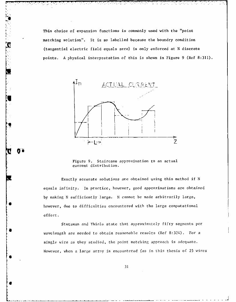
Each segment will overlap with adjacent segments to approximate the

current on the entire wire, as shown in Figure 11.

APPEL (QX._ CUR RENT

WL .

Figure 11. Five segment piecewise sinusoidal

ID Acurrent approximation.

PWSEF are chosen because the actual current is anticipated to be

sinusoidal, and therefore the closest approximation should be PWSEF.

The greatest advantage in using PWSEF instead of pulse functions is the

inherent reduction in segments. To obtain the same degree of accuracy,

Stutzman and Thiele find that "almost ten times fewer segments areI

required for the PWSEF as for the pulse expansion function" (Ref 8:325).

Therefore, using PWSEF, only about five segments per wavelength

are needed. This reduction, then, makes the study of a 25 wire per wave-

length array feasible using the moment method with PWSEF. Now, only a

125 by 125 array (250 by 250 for ground plane case because of image array)

need be inverted. This is possible for many computer systems.

33

In order to obtain the best possible approximation, the boundary

condition (tangential electric field equal zero) must be enforced as

"closely" as possible. The point matching technique is not an exception-

ally good approximation because the boundary condition is only enforced

at one point in each segment. Instead, a better technique is to attempt

to enforce the boundary condition in an "average" sense (as many points

as possible) over the segment. This is what is done in an approach known

as the method of weighted residuals (Ref 10).

A residual field Ere s can be defined astan

Eres = Es + Ei (46)tan tan tan

Clearly, the exact solution occurs when Er e s = 0 In any approximatetan

solution, E res # 0 ; however, the best approximation would be to maketan

Er e s approach zero in some "average" sense. This can be done by definingtan

a Weighting Function W (z) such that:n

Lf W (z)E reS(z)dz = 0 n=1,2,..N (47)

n tan0

The weighting function W (z) is similar to the expansion functionn

6 F (z) ; it can be any set of orthogonal functions. If the weighting andn

expansion functions are chosen to be the same (in this case, piece-wise

sinusoidal), then the technique is known as the Galerkin method. As

previously stated, this thesis ib using the Galerkin method; therefore,

W n(z) = Fn (z) . Then using Eq (46), Eq (47) is equivalent to:

L[W (z)En (z)dz + f W (z)Ea(Z)dz = 0 (48)n oa n ta0

34

{

I

Sii)-e a current on a wire will produce a scattered field Es, and

because there are only 2 directed wires, Eq (31) can be interpreted to

represent the scattered field which was caused by the induced current.

Eq (31) can then be substituted into Eq (48) for Es yielding:tan yilig

1LL n(Z ) [J-W-C2 (R) + a 2 (R)j(z')dz']dz

ni

L o 0

-f W (z)E dz (49)L tan

The right side of Eq (49) is recognized to be the "average"

induced voltage, V ; it will be discussed in the following section. Theq

left side is equal to the induced current multiplied by the cross imped-

ance Z , between the source and observation segments. It can beqq

simplified by realizfng that:

aa.(R) =- a- p(R) (50a)

.a aaz i(R) - az. 2 (R) (50b)

Using Eqs (50a) and (50b) in Eq (31) and integrating twice by

parts yields (Ref 8:329):

[ [p(R) I(z) + I(z) -- k(R)]

0 z

L [a_ -) +2+ 0 2 (z) + I(z )]'(R)dz (51)

35

Since the current is being approximated by PWSEF, for a single] "'- th

q source segment, Eq (51) becomes:

E % [ p(R) -L W() + F (R))• WE zZ q' q' z)3

+ o(Z) + 2F q(z')](R)dz' (52)

An interesting simplification occurs because PWSEF were chosen. Using

Eq (44) and twice differentiating, it is discovered that:

F (z') - 2Fq.(Z) (53)z2 q q'('

This indicates that the bracketed expression in the integrand of Eq (52)

is zero (Ref 9:370). Eq (52) then reduces to:

E [iP(R) F (z') F('z) Z (R)] (54)0 source

segment

Evaluating Eq (54) over a typical source segment (pictured in

Figure 10), and denoting the distance from the obs point to Zq -.1 Zq'*

and Zq.+l as Rql , R q , and Rq.+l , respectively, Eq (54) equals:

Ez j J [p(Rq) - F .(Zq.) + F q(z ) -L (R )

S q'- q q z q'-

+ ) Fq ( ) + Fq(Zq'+) (Rq )

q'+1 3z ' q '+ +1 q qz+1 az q '4-1

q Z qq q ''

36

I

The first and seventh bracketed terms cancel, and F q'(z q- )

F q'(zq =l 0 ,leaving

-Cs~ - z ' )-CO~

E p(R )L q q q'+ q')(z- -

z W: q sin (zq ' + zq ') sin (zq +1-zq

'q -1' sing(z z

q Zq~i

- (R )1 (56)q +1sin (z -zq

which, using the trigonometric identity

sin (ax + 0) cosctsinB cosfsinL (57)

can finally be expressed as:

E s -j 30fq - ZqR q

e R q'qlininz(z qq q'i)

e q sinl '+ 3(zIR qAsiB~zq' z q'-l)sinf3(z q'+i Zq')

+ RA e- Rq,+ (58)q+s inO3(z q'l- zqi

37

Then, the expression for Z - can be given using Eq (58):qq

Z = I ESdzqq obs q z

seq

[q sin(z - q-1) Zq+1 sina(zq+I z)fsinS~z z + f sin (Zq+ : Iq

Z_ q q-1_ q ) + qq

* e ~-JR -_ ' cosB(z - zq) -j R qJ • [j30(R e ls n ( q - z . ) 2 sinI - q .'

R q "sin(z q - sin (zq'+l qzq) R q

+ e- q+ ]dz (59)

R Rq+isinI(zq'+. - z q)

Stutzman and Thiele present a similar but less detailed derivation

for their simpler case of a single wire. Eq (59) agrees with their

result if appropriately simplified (Ref 8:331).

2.4 Induced Voltage by Incident Plane Wave

thThis section describes the q voltage matrix element, V q From_ q

Eq (49), the "average" weighted voltage is:

V = f W (z) El dz (60)q L q tan

E must be determined for a plane wave of arbitrary incidence angletan

with matched polarization, as stated in the initial assumptions. An

arbitrary plane wave can be specified by the "plane wave solution" to the

vector wave equation as:

E e+jpn 'r (61)0

38

where

E is a constant vector, to be specified0

Sis the propagation constant

n is the propagation vector

r is the radius vector from the origin

Since matched polarization is assumed, then E = E 0 , because0 0

the wires are ^ directed. By expressing the radius vector i in terms of

rectangular coordinates, then

E= E ^ e+j ((sinOcos )x + (sinOsin )y + (cosO)z) (62)0

so that:

zq sino(z - z qi) Zq+1 sin6(Zq+ I - Z)V - + f ] . zq Z sin (zq - Zq-1) z sin (zq+1 - Zq)Q-" q-1 q

" E + j ((sincosP)x + (sinOsin)y + (cosO)z))dz (63)

Now, both Z qq and V have been expressed in a form suitable forqq q

computer implementation (see Appendix A). Results for different wire

spacings, lengths, and incidence angles are given in the following

chapter.

I

39

I

III. Results

This chapter presents the results of the computer program and

compares them with the physical optics approximation. The parameters

investigated include: (1) wire spacings, (2) number of segments per

wire, (3) wire lengths, and (4) varying incidence angles. Unless other-

wise indicated, all results were obtained with the same set of input

values. These are:

Number of wires = as indicated

Segments per wire = as indicated

Wire length = 1.0 meters

Wire radius = 0.005 meters

X wire spacing = 0.50 meters#I wires04 Y wire spacing = determined by width of array

Frequency = 300.OMHz

Propagation constant = 27/X

Eo01 = 1.0 volts

Width of array = 1.0 A = 1.0 meters

The current is in units of AMPS, voltage in VOLTS, and length in METERS.

*G For each of the different cases studied, both current density

magnitude and phase is presented in either a "horizontal cut" or a

"vertical cut". These terms need to be properly defined for accurate

interpretation. A horizontal cut is the current on the center segment of

each wire across the width of the array. For example, with 5 segments

per wire, a horizontal cut presents the 3rd, 8th, 13th,... (Q-2)th seg-

* ments. Conversely, a vertical cut presents the current of the center of

40

L

the wire array for the length of the wire. For example, with N=5 and M=7,

a vertical cut presents the current on the center wire, segments 16, 17,

18, 19, and 20.

3.1 Wire Spacings

A fundamental question to be considered is for what range of

wire spacings is this moment method technique applicable. It is known

that the technique can be used successfully for a single wire case, as

demonstrated by Stutzman and Thiele (Ref 8). However, an objective of

this thesis was to determine if a parallel wire array could sufficiently

model a flat, conducting plane. This involves using "enough" wires to

achieve a "reasonable" approximation.

As was stated in Chapter I, it is expected that the moment method

results should become more accurate as the number of wires/wavelength is

ID increased. Results in Figures 12 and 13 verify this expectation to a

certain extent. The purpose of establishing these results is to deter-

mine if a trend exists as the number of wires is increased.

For a normally incident plane wave upon a flat, conducting iheet,

the physical optics approximation would yield a current density of.

Ei - e+jkx

-i I +jkx

376.7

.. ] .6x 5.31mA/m* s 376.7

This does not totally agree, however, with what the actual distribution

is expected to be. One would expect the actual current to be basicallyI

uniform (flat) across the center of the sheet, with per!hims a perturbation

41

II

17~ ~ 7>~I7 -

t~ :lmI

I~ T4 T' ....1

41 1 FTo v

* ~ r. 0

'' I I .- 4 CO~r

1 H '-H

~iI *42

I . . . . . .

. . .. .'.. O .... . . '

1 ' a'j " ' :° . .. . . i .. .: '

Cd u.i , l

i C (I U

> -4

.4-' '' I-. * 11 CUI * . ' "

' '. . . . . .. ,; r.. . . 0 . . . .

i .

~~43

near the edge caused by the abrupt boundary change. The current along

each wire (vertical cut) should be sinusoidal, with the endpoints of

each wire equal to zero.

It is evident from Figures 12 and 13 that the moment method seems

to be more accurate than the physical optics approximation. The hori-

zontal cut indicates a basically flat distribution across the center with

a perturbation at the edge, as is physically expected. The physical

i optics approximation is flat and of the correct order of magnitude, but

does not represent any effects caused by the edges. The vertical cut

is symmetric and sinusoidal, as expected. The current is zero at the

ends of the wire, but Figure 14 does not apparently indicate this

because the current at the center of each sinusoidal piece was plotted,

not the current at the exact endpoint of the wire. Note that the physical

optics approximation does not show the currents approaching zero at the

ends of the wire.

The current distributions also tend to "flatten out" in the

center region as the number of wires is increased, as expected. A word

of caution is in order, however. Although this flattening trend is

present through 36 wires/wavelength (which should be enough for most

* applications), it may not continue to exist for arbitrarily large numbers

of wires/wavelength. It was initially assumed that the wire diameter

was "small enough" so that there was no circumferential current variation

* on the wires. If the spacing/diameter ratio becomes too small, this

assumption may become invalid. Although the lower limit of this ratio

has not been identified by this thesis, good results are achievable as

9 low as (1/36)/0.005 = 5.55:1. This point may be an aspect of future study.

44

6

3.2 Number of Segments per Wire

As presented in the theory, more accurate results should be

obtained by using a greater number of segments/wire. Theoretically,

there is no upper limit; there is an upper limit imposed, however, by

the increased computational effort incurred and the available computer

resources. The question this section investigates is whether increasing

the number of segments (beyond five) is worth the additional effort.

*Figures 14 and 15 display the induced current (horizontal and

vertical cuts, respectively) for a IX2 array with five wires. By

increasing the number of segments, one would expect a more accurate dis-

tribution of the current along the length of the wire, with little or no

change across the array (in the horizontal cut). Note that the physical

optics approximation is unchanged for each case, since changing the number

0. of segments has no meaning with this approximation.

Results show good agreement with actual expected behavior. The

horizontal current distribution changes little in both general shape

and magnitude for all five cases. This is reasonable, since one would

not expect the current across the wires to be appreciably affected by

changing the sampling increment along the length of the wire. The verti-

* cal current also changes as expected. The midpoint current remains

relatively constant while the endpoints decrease nearly in order of

magnitude.

A This sixfold increase in the number of segments shows no signifi-

cant change in the horizontal current or the center region of the vertical

current, but does indicate the expected decrease near the endpoints of the

wire. Since it is known that the current must be zero at the ends of each

45

-ittit 4

4I, Cu

"' ~ . .. . 4 j.. ... i

-T . .. 44c-

t I o 44

,r w

, , , , / . .. . - ' ' ' ' .,,,

, 0... -

6.... ....... ...

. . . . . . . . . . . .. . . . . . . . . . .. . . . . . .,.

-I --:. . . -+"," ... ' " -- '" "

*!+! ,

' 46

Ii

1 1'- - - 7 , T-

t I '

I If

(JO ., 7

oj co 0

I CO4

4441

44--

~.lui'-4

-1~~t 4-4. .I4

-WI1

47a

Inr

wire, the region of interest is the relatively uniform center region.

Because increasing the number of segments/wavelength beyond five con-

tributes little additional information, it can be concluded that five

segments/wavelength is sufficient to obtain reasonably accurate results.

3.3 Wire Length

Figures 16 and 17 present the horizontal and vertical current

distributions on a iA wide array for four values of wire lengths. The

purpose of this section is to determine if the moment method will reflect

the expected changes along the wire length.

Results for the horizontal cut are reasonable. All four curvesI

are symmetrical with respect to the center wire, and tend to flatten out

as the wire length is increased. This is reasonable, since as the array

size is increased, one would expect the edges to have less of a distorting

effect upon the center region, thus allowing the current to become more

uniform. The decreasing trend is explained by considering the vertical

cut, Figure 17.

Currents on the vertical cut also change appropriately as the

wire length is increased. Figure 17 indicates a trend to form two main

lobes (d) as the length is increased to 2.OX, which seems quite acceptable.

As these two lobes are formed, the center segment (#10) value must be

decreased accordingly; this in turn causes the decrease in the horizontal

cut, Figure 16. Therefore, the primary effect of increasing the wirealength is to cause the appropriate number of lobes to form along the

length of the wire, and to cause the horizontal current to shift accord-

ingly. Note that the physical optics approximation reflects no changeI

in eithter rutt ns the wire lc n,,th i. incrua-ed.

48

0

-. 41

14--- -.4

44 >

*~~ I v4

4 I4

40

0

V$ 0 ~

*

40

494

t T

. ~ ~ ~ ~ ~ ~ ~ ~ 1 .. .. ..- . . .. .. . .------

.4

.- . . . .. .

ca_ _ _ _ _ _0 -- 4--~

. . .. : . . ., 0 r4ji~7~

- -- 0 4j r- % 0 c - -C

. . .... 1 . 1 ..2

- . .- .~ .. . t *r 4

. . . .. . . .L .4 -

q-4~~2- C .. ..

. .1 . . .

3.4 Varying Incidence Angle Effects

The horizontal and vertical current distributions are determined

for different sized arrays when the plane wave incidence angles (0, 4)

are varied along their major axis, i.e., when 0 is varied and =0, and

when 4 is varied and when O=rr/2. Phase plots of each are also included

in this section, since there will be phase variations in both cuts.

The first array considered is IX2, using 26 wires of five segments

each. Results for this example are presented in Figures 18 through 23.

For 0 variations, Figures 18 and 20 present the horizontal and vertical

currents, respectively. Physically, one would expect little change in

shape for the horizontal cut as 0 is varied, since all segments will still

S- lie on the same phase front for all O's. This is exactly what is shown

by Figure 18. For this and all other examples, the physical optics

approximation of the current and phase is calculated by:

(sin)E "e j((sinOcos)x + (sinsin )y + (cos0)z)

with i = 2E 0 (snsn)y+(o0z (64)

- 2E(sin0) (cos4)then !Is =

- 7. (65)

s 376.7

and (xsin0cos + ysinOsin + zcos0) (66)

For each 0, the physical optics approximation is of correct order of

magnitude, but does not represent the distortion of the current near the

edges.

The currents for the 4 variations, Figures 19 and 21, are also

in agreement with expected results. The horizontal current is symmetric

at normal incidence, and varies as 0 is varied. Note that the physical

optics approximation shows only a shift In magnitude, which does not

51

11 IT

oo4,

4~ 1 iI~~~c n:,,,* ~

. . . . .. .. . . .

0 CI4J

a 0

. . .. . .0) U-.4

i 1.4

.u . .I

52

..... ....

,.I 4i 4-.

M11 1

I~~ , .,4I

.4 cu Im

53 I

U6-

p-77

TII

!!LT IJ IiU

-I J .C

j ~A.

4 4-I 14

-44 I 1

. . 1

"N- --

54

110

C: 0

IIn

04-

-5

I

WV

tN

0 u

I .. K..W 3I~~ 0tt.U ~ ~ ~ ~ ~ ~ ~ ~ ~ : o}14'*-~---~~-4~~...

~-> L~JKo

Fn .:. . ca w

0 41

4~~~$ -H:: *1 i

04 C' .' . .

56

*~c 4.), .~0 AVU(A uj

I, w

i-' a)jt 17 -

. . . . . .. l

1 C1 C4-4

57:7

aJ

seem to agree with actual physical behavior. The vertical cut of the

current, Figure 21, however, is symmetric for each case. This is

entirely reasonable, since a change in the 4 component of the incident

plane wave would not be expected to affect the shape of the current in

the 0 direction. There is only a shift in magnitude, which is probably

caused by the change in the horizontal current.

The phase relationships for both cuts are shown in Figure 23 and

gI 24. As expected, the phase in the horizontal cut is dependent upon 4,

but independent of 0. The physical optics approximation predicts a

linear phase change for each as shown, which is calculated from Eq (64).

The moment method technique also indicates a similar linear change, with

a slight distortion near the edges as shown. The vertical cut of the

phase, Figure 23, is also reasonable. As expected, there is no change

I Iin phase for variations, only 0 variations. The physical optics

approximation predicts a linear change, as shown. The moment method

results show a similar, but not exactly linear variation, which may be

caused by reflections from the ends of the wire, which will tend to

induce a "standing wave" on the wire as 0 is decreased.

A second case was also studied to investigate current behavior

4on an array for various incidence angles. Its dimensions were chosen as

IX wide by 2X long (13 wires of 10 segments each) to determine the

currents, especially in the vertical cut. Since the previous example has

4 already established that the horizontal currents are independent of 0,

and the vertical currents are independent of , these graphs are omitted.

The horizontal cut, Figure 24, indicates a definite change in

the distribution as is changed, a; expected. Again note that the

58

- ~ lr .4 : : .. . .. . .- .- . .

I M4 . . .:

,.III4

I I.] 4

0 ® ICd

.4c 14

oa

z.%:

~~V4

59-

physical optics approximation reflects no change in shape, only a shift

*in magnitude. Also of interest is the fact that the relative changes

in the horizontal cut for the moment method results are less than the

corresponding results for the previous example (see Figure 19). Again,

this is an indication that the center region becomes more "isolated"

from current variations as the size of the array is increased.

The vertical cut for 0 variations, Figure 25, is also reasonable.

The current for normal incidence illumination is symmetric, and has the

two-lobed structure, as expected for a 2X long wire. As 0 is varied,

the current becomes asymmetric, and in fact resembles a standing wave

pattern. The physical optics approximation shows no change in shape for

different O's, only a shift in magnitude.

The phase relationships for this example are shown in Figures 26

and 27. The horizontal cut of the phase agrees well with physically

expected behavior. For changes in 0, there is no change in general shape,

only a shift in magnitude, as expected. As 0 is decreased, the rate of

phase change across the array tends to increase, indicating that the rate

of phase change is proportional to the incidence angle. The vertical cut

of the phase, Figure 27, shows similar agreement. Changes in have

little effect on the vertical phase, except a small shift in magnitude,

as expected. As the incidence angle increasingly deviates from normal,

the rate of phase change increases proportionally. Note that the physical

* optics approximations predicts an exactly linear phase shift, whereas the

moment method predicts the same general trend, but also includes minor

variations and distortions near the edges/ends.

6

60

I

. . . . .. .

~j -. :

. ,OK-

u 0

4 uc4

"1 0

I~ 4-4...

.. V .

I' .. ~ II 4

.. (.. .- .. . . .

4 I::It::61

a(

F (~) (~) . 44

. . . . .(J 1

14 ..

JT; ... ... -

Pa.4 .ii iI4\

*i~I F I ria

62l ~c

7.7 7721* s*4'

l\ I

. I 0

~ . . . . . .4 >w

i'i* :: .::

v J0

44

ja i v'.' ' : 1 .. . .I : . :' : " '

> C1

_-- - _.. .. " _ " _ ' '_-"__ - ... .- . .. . + ->' '-,-

-I . . . . . . . . -.. . . . . . ' i . , m- 4

4-

63 V

4P

4C) ... . ..+, ,7 . I +

-+ -t, t --t- -- . . .t . . . t I ' + " I + . . +I ' + ' . ...6 3- ,

3.5 Array 0.25X Above a Ground Plane

*The current magnitudes and phases for an 18 wire, 5 segment

array 0.25X above a ground plane are presented in Figures 28 through 31.

Again, because of the independence of 6 and horizontal currents and and

vertical currents, these graphs are omitted.

The horizontal cut with varying 4 is shown in Figure 28. As

expected, the normal incidence case is flat and symmetric, with increasing

changes as is increased. The interesting point to consider is how

these results differ from a same sized array not over a ground plane, as

Figure 19. The physical optics approximation for the two situations

(both over and not over a ground plane) are the same. This is because

the array is being modelled as a completely reflecting ground plane itself,

which in effect completely shields the actual ground plane behind it from

(04 the incident wave (at least for normal incidence--this is not true for

all incidence angles, and this point will be elaborated upon subsequently).

The moment method technique shows that the current in both situations

have the same general magnitude, but that the current on the horizontal

cut of the array above a ground plane increases at a greater rate across

the array. This is reasonable, as one would expect the ground plane to

UI reflect the incident wave back onto the array and increase the current

density.

The vertical current cut, Figure 29, is also somewhat different

4 9 than its free space counterpart, Figure 20. Again, the physical optics

approximation is the same for both situations. The moment method

results, on the other hand, are of the same general order of magnitude,

but are different in shape for each situation. Here again, the moment

64

7 .7

4-1~

r I f

C1r4

4-41-

it 4-4.9 K KN Iii

0 j-~ Ar

40 to'0

.. .... ....$

65 .c

I0

pi4 I.L

I t V4.

~ . 0

o c

i 0.c'-I

4

4 b.o

-I66

II

~4

t toV

0 0>

I W91044o

I1 0'-

44I0 wb

L~l '. r ,0

I I; 67

..... i.. .....

* ... ... 00~4 244

4.''

.1 .... . . . ~ 0

.........................

I! ~ : 1 *o

42) Q. . T

~0 / 1 1o.0

-4 Q)

to cn

68

method results appear more accurate than the physical optics approxima-

tion, since different results would be expected for different situations.

Similar conclusi as can be made concerning the horizontal and

- vertical phase relationships for both situations. The horizontal and

vertical phases for the array over a ground plane (Figures 30 and 31)

are expected to differ from the array in free space results (Figures 22

and 23). Again, there is no difference between each for the physical

optics approximation. The moment method technique differ, as expected.

An important point of the geometry of the problem should be

noted. As was previously stated, the physical optics approximation

models the array as a conducting sheet, and therefore, the actual ground

plane is completely shielded from the incident wave at normal incidence.

At any oblique angle, however, part of the incident wave will pass by

the edge of the array, and still illuminate the ground plane; this in

turn may then be reflected back onto a different section of the array

(see Figure 32). This effect is not accounted for in the results of the

physical optics approximation as presented in the previous example. To

properly account for this effect would drastically complicate the

presently simple approximation, and would therefore defeat the whole

* purpose of using it. The moment method, on the other hand, has already

taken this effect into account by virtue of Image Theory, with no addi-

tional modification or complexity.

6

J

00

tko

CL4J

IC 0

004

*1-4 Q

I-I70

IV. Conclusions and Recommendations

4.1 Conclusions

The objective of this thesis was to determine the induced currents

on an array of wires both in free space and in front of a ground plane

using the method of moments, and then to compare the results to those

obtained by the modified physical optics approximation. The induced cur-

rents for the momciL method were determined by developing a general algo-

rithm (Appendix A). Results were obtained for a variety of different cases.

In general, moment method results agree well with expected physi-

cal behavior, but do not agree closely with the physical optics approxi-

mation for most cases. The moment method and physical optics approxima-

tions tend to agree in general magnitudes, but sometimes differ signifi-

* cantly with respect to the general shape of the current distribution. For

example, consider an array illuminated by a normally incident plane wave.

The physical optics approximation would indicate the current to be exactly

uniform across the entire array; the moment method shows relative unifor-

mity in the center region, with a perturbation near the edges. For this

case, the moment method appears to be more accurate, since one would

* physically expect a deviation near the edge caused by the abrupt boundary

change.

Also, the physical optics approximation shows no change in the

shape of the distribution as the incidence angles are varied; it only

reflects a change in magnitude. This does not appear to be physically

realistic. It can be concluded that the physical optics approximation

does n'et adequately represent "edge" effects. The physical optics

71

approximation also does not reflect the fact that the current must

equal zero at the endpoints of each wire. It does, however, produce a

reasonably close approximation to the current along the center region of

the wires. From this, it can be generally concluded that the physical

optics approximation may be useful for larger sized arrays, to obtain a

"rough" idea of the current magnitude, but not useful to determine the

shape of the distribution with any great degree of accuracy. Its

u greatest advantage is in its simplicity. For a large enough array, it

provides a good idea of the current magnitude with minimal effort.

The moment method, on the other hand, requires considerably more

* effort (i.e., large matrix inversions), but appears to be far more

accurate. The accuracy can be increased by increasing the number of

wires and segments, but this cannot be done arbitrarily, since there will

! 9. be an upper bound imposed by the available computer resources. However,

reasonably accurate approximations of the currents are obtainable with

a modest number of segments, as is evidenced by this thesis. Some other

conclusions of the moment method technique are:

1. The accuracy of the solution tends to increase as the wire

spacing is decreased, i.e., as more wires/wavelength are used. Reasonable

* results are obtainable for as few as five wires/wavelength, but as many

as 30 wi I provide an obviously better result. The reader is cautioned

that the wire spacing/diameter ratio mny not be decreased too small,

* since doing so may invalidate the assumption that there is no circum-

ferential current variation on the wires. A]though this -hesis made no

definite determination of the lowcr limit of this ratio, good results

72

ii ( .. . ..-. ' .. ".... . -. .-.-.. "- ". -.. ".-"--.--.'.".-.. _".'.i ":"; :- '.. ....... ... : . -: .. ".

were obtained with a ratio as small as 5.55:1. The actual lower limit

may in fact be substantially less than this value.

2. The accuracy of the solution will increase as the number of

segments/wire increases. Although there is theoretically no upper limit,

little additional accuracy is gained when the number of segments used

is increased beyond 10/wavelength. However, very reasonable results are

obtainable with as few as five segments/wavelength.

3. This moment method technique appears to adtquately represent

the various effects caused by changing the wire lengths and/or incidence

angles of the illuminating plane wave. Results indicate that the current

distribution develops a second lobe as expected when the wire length is

increased to 2.OX. Also indicated was the independence of the horizontal

current to changes in 0, as well as the vertical current to changes in 4.

The moment method also indicates the distortion near the ends of the

array, the trend toward zero current at the endpoints of the wire, and

the different distributions of current for the array in free space as

opposed to the array above a ground plane. The physical optics approxi-

mation reflects none of these.

Thus, the moment method works well in approximating the currents

*on arrays both in free space and near a ground plane. The physical

optics approximation provides a very "rough" idea of the current magni-

tude at the center of the array, but does not reflect maly of theKimportant aspkcts of the shape of the distribution, especially near the

edges/cndpoints of the array. The physical optics approximation may be

more useful for larger sized arrays, however, where the center region

is more independent of "cdge effects". For smaller arrays (on the order

I "

F'

of the ones in this thesis), however, the physical optics approximation

does not provide a very accurate solution.

. - 4.2 Recommendations

" "Although very good results can be obtained with the values used

in this thesis, even greater accuracy may be desired. To accomplish

this, one may choose to incorporate a larger number of wires/wavelength.

As previously stated, this may invalidate the assumption that there is

no circumferential current variation on the wires. Therefore, a logical

extension of this work could be to better determine the lower limit of

the wire spacing/diameter ratio. Or, perhaps even better if possible, to

exclude this assumption entirely and rework the theory to account for a

possible circumferential current variation.

Secondly,, the major disadvantage of the moment method is the

large, time-consuming matrix inversion required. A paper was recently

published (July 1982) by Kastner and Mittra (Ref 9:673-679) describing

a new spectral iteration technique which analyzes a similar problem with

no large matrix inversions; instead, it employs a Fourier-series

approach. Possible future study may include a detailed comparison of the

two techniques.

4

74

Bibliog aphy

1. Richmond, J. H. "Digital Computer Solutions of the RigorousEquations for Scattering Problems," Proceedings of the I.E.E.E.,53: 796-804 (8 August 1965).

2. Mei, K. K. "On the Integral Equati~as of Thin Wire Antennas,"I.E.E.E. Transactions on Antennas and Propagation, AP-13: 374-378(3 May 1965).

3. Richmond, J. H. "Scattering by an Arbitrary Array of ParallelWires," I.E.E.E. Transactions on Microwave Theory & Techniques,

* 13: 408-4 12 (4 July 1965).

4. Wait, J. R. "Reflection at Arbitrary Incidence From a ParallelWire Grid," Applied Scientific Research, 4: 393-400 (1955).

5. Michel, Yves, Pauchard, and P. Vidal. "Diffraction of a Plane Waveby a Finite Set of Cylindrical Conductors," 8th European MicrowaveConference Proceedings, published by Microwave Exhibitions andPublishers, LTD., 1978.

6. Richmond, J. H. "A Wire Grid Model for Scattering by ConductingBodies," I.E.E.E. Transactions on Antennas and Propagation, AP-14:782-786 (6 November 1966).

7. ___. Computer Program For Thin Wire Structures in a HomogeneousConducting Medium. Contractor Report for NASA, # CR-2399, June 1974.

8. Stutzman, Warren L. and Gary A. Thiele. Antenna Theory and Design.Canada: John Wiley and Sons, 1981.

9. Kastner, Raphael and Raj Mittra. "A Spectral-Iteration TechniqueFor Analyzing a Corrugated-Surface Twist Polarizer for ScanningReflector Antennas," I.E.E.E. Transactions on Antennas and Propaga-

tion, AP-30: 673-676 (4 July 1982).

10. Schelkunoff, S. A. and H. T. Friis. Antennas--Theory and Practice.New York: John Wiley and Sons, 1952.

11. Finlayson, B. A. The Method of Weighted Residuals and VariationalPrinciples. Now York: Academic Press, 1972.

-75

I

.7

I iBbligah

Appendix A: Computer Program

This appendix contains the computer program. Included below is

a brief description of the general development and operation of this

program.

DEVELOPMENT

Before beginning, it should be noted that a program (for a single

wire case) has already been written (Ref 8:568). This program, however,

is significantly different; it allows for the more general case of wires

located near a ground plane. The major difference between the two pro-

grams is that this program does not inherently assume that a (block)

Toeplitz matrix will be obtained. It does not exploit the fact that a

Toeplitz matrix is highly symmetric (and therefore more easily inverted);

in fact, it assumes the most general case that the matrix is totally

asymmetric.

The program actually solves Eq (43) using Eqs (59) and (63). In

order to accomplish the matrix inversion, it calls upon the International

Mathematics and Statistics Library (IMSL) functions DCADRE and LEQ2C.

The IMSL is a set of subroutines which should be available at most com-6

puter installations. So ne minor problems developed with the use of

DCADRE, however, which are worth mentioning.

DCADRE is thc IMSL subroutine to evaluate a real integral, given

the integrand, the limits (finite), and the maximum allowable error,

AERR. The problem oczurred in trying to use DCADRE to evaluate the

complex integral in E-i (59) and (63). The solution used was to break

the complex integral into real and imaginary parts, evaluato each

76

separately, and then recombine into complex form. Also, because of the

repetitious nature of the integrand, several common terms were extracted

and made into function subprograms, as shown below.

z)

qsinB(Z - Z)-30 q 1 [BCTdzAib

INC sin( *DZ) zf sin*DZ) BC ldz(-a

I q-

IT -30 zqlsin (Zl- Z)i

IND sin(f3*DZ) Zq 1 sin( *DZ) BCTdz(-b

z30 +q sin 3(Z - Z

INTF -3[+ BRCKT2]dz (A-id)sin(f3*DZ) z sin( *DZ)

ITta Inega =3 (T + N)+ q(NT + INKTF) (A-2)

sin(* 1 2cosU*DZ)sn*R )

qq

sin *Rq 2os(*DZsinG *R )

+ gi*Rq+) (A-3a)

77

BRCK2 = cos( *Rg._I) 2 cos(O*DZ)cos(B*Rg )r.BRCKT2 R q R-

qI q

cos( *Rq-+l)+ } (A-3b)

Rq+

and Rq-I Rq and R are evaluated by functions RBOT, RMID,q- ' q q

and RTOP, respectively.

OPERATION

The program was written in FORTRAN V. It requires the use of

IMSL subroutines DCADRE and LEQ2C. Because of the matrix manipulations,

it requires a larger than average amount of memory and CPU time.

Although the amount will vary depending upon the system used, the user

should request approximately 256K words memory and 9000 seconds (150 min.)

Q.O of CPU time for a 250 element array.

The user should specify N, M, WSY, etc , according to the input

format statement. The output is dependent upon the four control param-

eters SWEEP, PV, PZ, and TYPE.

SWEEP must be an integer value 0 or 1. 0 indicates that only an

incident plane wave of normal incidence (THETA = 7/2, PHI = 0) will be

6I evaluated. I indicates that the incidence angle will be varied in 7r/16

increments along the THETA and PIl axis from 0 to r,/2.

PV must be an integer value 0 or 1. 0 indicates that the voltage

array V .(q) is not to be printed. 1 indicates print V .(q)q q

PZ must be an integer value 0, 1, or 2. 0 indicates do not

print impedance array Z . 1 indicates to print only the first row ofqq

78

.______

Z - . 2 indicates to print entire Z - array. It is recommended thatqq qq

option 0 or 1 be used, since 2 can produce a tremendous amount of unneces-

sary output.

TYPE must be an integer value 0 or 1. 0 indicates that the free

space case is to be studied, i.e., no ground plane. Here, Q=MN so the

DIMENSION statement is MN in magnitude. 1 indicates the ground plane

case. Here, Q=2MN, so each array in the DIMENSION statement should be

accordingly doubled.

NOTE: WA and WK arrays in the DIMENSION statement are work areas

for the IMSL subroutines. See any IMSL Operator's Guide for further

details.

79

4

READVARIABLES

MEMORY

.PRINTDAT RRt-MOR

ERRRSBMESSA

NO

DATA OK, PRINTIT OUT FORVERIFICATION

IEFIMWIREGEOMETRY

PRINT ITOUT FORVERIFICATION

__ _ BEGIN NESTED[DO LOOPS

CALL SUBROUTINE I YCOORD (SOURcE"SAWIR" TODETERMINE. IF YCOORDj9OBS"OBS" & "SOURCE"SE G E N T S A RE O N S 'T

4 Figure A-I. Computer program flowchart.

80

I

PUT CURRENT [SU nINEVARIABLES INTO "SAMWIR"J-COMMON FOR USE

BY OTHERSUBPROGRAMS

CALL SUBROUTINE"INTCRL" TOCALCULATE Zqqo

_ ER__ "INTGRL"

-- IMAGPT. _PRINT Zqq'

ACCORDINGTOPZ

- -- ENDOF-NO ~DO LOOPS?

_ _ _ _J.YESrsF'~VA TUP F)67THrTA &PHI

LACCORDING TO SWI.-EP

* BEGIN "OBS"

[DO LOOP[CALL SUBROUTINFE -BJERR I"VOLT" TO "VOLT"CALCULATE V "VOLT"AL

q - -VIU-'

Figure A-I (Continued)

81

. . .I % e i 1 " | -

74

PRINT VqACCORDING

TO PY

NO E-D'-LOOP?

[i" .o.... m o- --I

SMATRIX EQUATION SUBROUTIN.. ~~~~~~BY CALLING MATRIX I L--IQ2I--.SINVERION SUBROUTIN -:.EQ2

I[4 Sl LEQ2Cq

ANOTHERTH1 rA & PIlACCORDINGTO SWEEP?

END OFPROGRAM,STOp

Figure A-1 (Continued)

82

RERR _-- SUBROUTINE "IMr'RL"IER __ __CALLS FUINCTIONS INTCt INTD, luTE, INiTF,

RE-ALFr--- EACH A SEPARATE TERM OF THE COMPLT= INTEGRAL.__IMAGPT_____ THEY IN TURN CAL.L IMSL SUBROUI?&, "DCADRE'

4 WHICH IrnEGRATES nT!.M BY USING TEE RESPE~CTIVE-- t> INTEGRANDS FUNCTIONS4 C. D), E, & F. THES ARE

WRITTEN IN TER M OF FUNCTIONS "BIRCKT1" &'BRCKT2"p WHICH ARE FUNCTIONS OF THE OBS TO

SOURCE SEGMENT DISTANCES 'RBCOr", 'RMID"t

~fi~}~-~ R~74-+FUNCTIO3N C 4

~INTE~ +--- _ _ C --.EFNCTION D

b, [{IFt4 1, tDADRi U4 ~ NCTION F~

44--------------FUNCTION1 FUNCTION"BRCKT2" V"BRCKT16'

[RBm. , l-MIDI RTOP! IRBOTJ RM#11 FRTOPi

Figure A-1 (Continiued)

83

D-A125 646 ANALYSIS OF THE INDUCED CURRENTS ON A SECTION OF 2/2~PARALLEL MIRES IN FRONT 0 .(U) AIR FORCE INST OF TECHhS RIGHT-PATTERSON AFB OH SCHOOL OF ENGS! T M SODOWSKY

UNCLASSIFIED DEC 82 AFIT/GE/EE/82D-35 F/S 9/1 NEhhhhhhhllllllhhiElEhhhhhhhhhhhhElllllll

1111. I. kg 2.11.

11111.2- 11 -

MICROCOPY RESOLUTION TEST CHARTNATIONAL BUREAU Of STANDARDS- 963-A

__HERR- SUBROUTINE '"VOLT"__ I__.i ' CALLS INTVl, INTV2, INTV3, & INT ,

VRAL -- EACH A TERM OF THE COMPLE~TE INTEGRAL.

':-. ~-.- - .--J- J . .. .""MA "DA "ISCLETOIEGAEAH

UINTH 4NMGAND V{ Vo j1 V4AODR

-- -

-DCADnH"l4V-V4

Figure A-1 (Continued)

84

I4

U C.

L LL

,a. I-"

c LL.

- .-- Lk ..

U >. . Li.

% - L LL-,

L; LL.

U C.C

C(6 Ll L-

J 41 C .C UL

S. ' .. , - - a -

1 ... .-. - . -' .- LL .4

_ L LC L'a_ a.! . . . C- " - .( - ? .

LA-

U L a S . Cf L L. LL C.~I- I

;.i. . .Ii ' L C

C.o t Va

a:V C C-~-~ CL: C.C L . L. ' - 1

L; tL- L.)L L 4L U L Q U LJ

Figure A-2. Computer program.

I (885

-

".,,.

c.

* LL

C r

, C - > LL

N LL

LL ZL i- L r- a-- <

-. -N. -I .. ..- 2 _

C, . p. . . .- , Ju.

r- -L

-L , .. -. &- • b r . - .

Ca - .-t L_ .- .-, .. -- --.. €-- C. .,' i C .,,--.-

," -'1.' .:--c , .- " - ( . -. ,. ~~ .L.' - CJA " a- . L.Cr- " '."

ii _ (..1.. .,. a A ,a.. r C. .L.-J L, L

V , U A A- L IL l{ A C .-. i-, ,-I- - c- c- I. . A A L: ,.C

L I -- -1 4

cf.C' U

"a &--- -. A' A-

[.r,1 , Cr. " C/ "r C., C. C. .. C. C, . C,.. - I- I, Z .. -, *, *'U,

r- L L- -

L CU. L CL) L. L- L~ . L LU U U L;) L.) C.) U. U. L; L-o L. L, L . L U. L.

0' td) .- ' kCU 'c C fl -, Z- V) 'kC- t. a r- Q. C. - C r.N t-' Ki W r , P ' K re,~ K ZC Z7 - Z 'Z Z ZZ Z ;II. If. CF IJr

Figure A-2 (Continued)

86

C

rL r -

.

-- oofIL

L -

Ck - ' I-

I.- L

C . C - c- - *-

Cr- U Ef a a f c - L:

L.. . r C. L, L- L.

. . .. .~ . L. -

'- OL C .-

, -.. .-

V . J- V. . C .C- U-. t- f rL - r

C,,,. ,,It-,.i ,.,-

"*j *" _,L "" I _-" L" i . .. .J ..

rZ ,il LI .IC f 4. .% .IC. .. . . £ Z. "-".. I I r b.- s I

I Figure A-2 (Continued)

87

- ~ -- 4~ .~ - '-~ - - !

(

.o.

'.i .

L C

L.r" r

tI--I I C I C.*

V- U.9~L

-, L. I-- I

* I. . L It"

L- It, -

. L h. - / . L i. % U .; ." U

> L L- L- II

C,..2 LU ..

LL a. ~ A L.

- .. u .- r\ r, r.,

3-. , . . .. "L - .3 - '. ,-- " C' C" . .. - C . :.

L C - C- Cs - -*C

LL LLL LL

CL. Cl. C.. CL CL. (t (- (. Cj. Q~ c. v C V 00 C c C C

i~ Figure A-2 (Continued)

88

LLI

C

w- .- I.-

c' -- LL

t- r (.. 1

M L -

L b

Ll i .v- 1A - L C, c-

g L7,.- C

V L. ~ L

ClP~r - L. C- C C C._ C ;.-

o Ca

:ZC 6,. 1 0. Z .r- I'-

(.: <- P' LiL'-( C- IC- - -P -rlf

-. - -- --..-. -. -- - --

Figure A-2 (Continued)

89

* ' b--- -- *.-- . - ---------i--S.T.

LA.

C:

LL -

LL.-

zL Ii

L C :* ""L - t7

I=.

• c C .-

,, I- -

-: - .

i-+. . + " .-- __.~ -

-' L-' L L L. L' C-

r .. _-." .. ; ,

G Figure A-2 (Continued)

90

!- *

bL

o.

CL

c C

C. l.'

.

-1.. --- .

L : ". a-. ,,-- e-..

- .. . L .

-- T'1 - . --

IL

L -, it. - ,. -

L '

o.~~~0 L,. " C T

v* €r

C. . ,-

It€" r" " cO 7- .L - c- LL it c" - C,- '', -

. eLU a

i-c.. . .

L: L L. L., L, L1 U. . L' . ' -,

, 1 £ d t* sf , ,Z aC C -- , ,

- - - - -- -- -

~Figure A-2 (Continued)

91

L L,

[U

2C. C-L .

'V,,- *r . .r

L, - ..

CL tS LL~ C ,* -L

Lk- U- II -. -- L Uu-U

-r k1 F . l

C* , 2 C. -- , r- r - e

-- - - - - - - - -- - - - - - - - -L - . .- N

92"

r- I -- 0 -r -' .. d 1. - " C ..- "- - "

k - ... ' .z L: .. .. .-* .. :. .. - . -J "

U. ' I -;' ,LC I,-_ . >. ,-)>

1, .> *" L.-.:

j~-. C'~c.II~--L- ~ t. -.

Figu- re -2 Continued) c..

X ? - a 92

~LL

V.. (I L

L L

C. c

Ll L-1> L.

c- L

C- L. - L: L LU **'

,J U .1 1- , ( - > C- 6 L- C- L E

C, Cj L- L; C- LL L~ W V;- - -C LQ-

z .. L - 1 , a. c --T U) 4; U I

C, ~ ~ J r, C'c.c Uk ,f, , r, ,r

M N (,r,.r rr. n, .- n-r. ut rjr r, v M %. 4

4LC $C - ..a-- C igur A-2C (Contin.Cud) L&(

(WCC .u( )' I

93

L L

C

.L. A t - L

LL t'

C-.

LL C C- L~. Ccr .. j LA. I-.V

L L

9-~ Lt C... .- C.

c a L- C..- I

-- C. V.

U." C9 L C L C

C.- LI.. '-6

*1 LI > L *~~-

Li-

I--. bCC- LL A L L-

0' - C.' Cy C -r -Lf

Figure A-2 (Continued)

94

C- c C

F--L LL L L.-L .~ r-

CD c-c cr.- c .

I .) U W. t., z*

I, - .L * - -L

- iL.LLU L L. I'

-~ ~~~~ L.-b- U s..

-~~~C L -~UJ~

(- L' L-L C. I * . * . * * L .--- '

'.Z C, C- - -Lr : U 'rU V L '' - 4 -,I,- r-

r\, - -Q rc r, q. . A r- m,~ N- rA- r- r.~ r \

Fiur A- (Cotined

C U' - C . -'a - p-b-a. .--9-5.

* .. '..

- J

.-.(V

--II

•~V • #

'I f - - o.- -.,. r

L L-

L . -L

"" " "* , . " -" S . ... '. " ._ 1.

C t1- LI

L- - -- t . - L t_ .

,,. ,.. S. S 5 I-- 5,- ,. I' -: *- C - -

Z,' -" L!,<, , L

LL C C C C L

to-' cf- Cf of" a. z*,J .. ,. CcM. r\ - -r-, r\-

+C - A :, C- ,: - " - L+ , C'; . ; ,:

1 Figure A-2 (Continued)

96

L V ": -

. ... ,. . • .-;. . ',. . , _

,-L, i _ .-. I. -I-.- C (2L'. ,- e

• - . I - ". e ._ L - . .- ,-.

u. v

-. . - i. II II7 i. . C , - t I '

*C L L..

r. I,, -- .' -.'JI. ,. ,_' I " . I.... ..

c LLa

- C - ~ C, "'--

14 I * I- , i . I II.. II *i C I !

* '-ut T A- ( .n Inucd)>- ~ ~ ~ ~ .LZ.IL ... ~ Z. I

I-- " - C .. .. C ' I- i-"C-r- n

7. LO

I.- LL) C. ~ L

L uLLC uLL LL C.LJL.

Figure A-? (Continued)

97

. -

*C.Er.

L

4.C L

A.3 ~ 9. c ~ V

-- C 6-

61 U.. --L2

,.c U. - .

c.:) j P, E.Qt L. UC .. '

c.' r,- r/ z.3 L- '- r- -1 r\ t

?I'- I- * C Li. ff 9-- r." f z :7 :7 L;

4e 4 )W .r.r;f rCL L -L 2 C V.~ -fe f4, r-Z rd r, e ^

Figur A-2(Contnued

98.'L' .1 ~&C C

r- ii I

>. C..

4 c'

L. LL 5 u.

LL.

-Itt C' .2Ll zr.; fr

L. C LL.

C: c -L: Cr ;, - 'V

LL- Le -r -rL -- r- x r z < cr. . - u tC, p ~ e e w r, w 4 v -;P1 t,-w - ~irr

Fiur A- (Cniud

* L N. s- 99

C..

r-.. . I- -

. CL LL

C. .. L

C'- *-I ' .r

r-L .LLL

- oC* ,.' ,,(1 , ),I

- .,L, t . '

* -*. . . _C .- c- C

C:

. , - - u

L L

. .L L ' nw J L L}L ' Lb U- -- L-"

I. U .-*I ,... P" . C . si - -. ,-

"- .~ : --.

L- L -!5

.I K L

L W uC.

L,.r

I7

o. a- a'- I--. LL L LL L

L;. L: L. L ILU

LILbLL L- - t

'-..JZ Lr C, cA N W- )I ~ :

C. C. C a CLCC C C (/.-~

Pf r4, I" r"-. ., LCL.J F .JL.. Ln KL f4

6 *~~'-9-- b-Figure A - (Continued)i~---

U100

.- -j 'V

P..

L L. Livi

L *.-.--

. -- -: -.- - -. -..

-LiT

LL_ ,, L I. LALr. *

LlL -

- - - -, . *-= .,. - .*. .s-- S= 1

- C. ,= E. , .-.. -. c -; c.

~~~'~. I). i I !5 .~~ , -

4 . C *- .- L • - N ' - -. .-~ , I

C_) +,. i fL. C. L . ' C - L- _ C.J "... . C -- L... " C. L. C

..

t + CL C" - ('i. . - L I,-.- a: C",,. - ( VL " L I - i r --

+ -..,.- Y " li - .- - - - -r J I r. . .\ r. r ,- ," r . r ., . r_.

.LL L, A/ L.

€,..,U I.-I.

~Figure A-2 (Continued)

101

44

L

4L

c - Lp.-.

S.- S o .,

C,,

7 r:

LL C'L.

U L.' Li CYC L L* 4-

rv.

SL- L L . .

-. 6- 4 . '- - 1 ,. - 'P ; JU -1 C...C ItL LL L . .

C. L, L. L L, C* ;C

(1 U L* U t-L: Lj

e .e i e - •,N * e fIlk C7 Ln -.. 1, C-

W- C Z P.?' ZZaz 4r -Z Z

Z: L :3z Z:TZ zZ 4 -:Uz Zz4z zz

~Figure A-2 (Continued)

102

77,

Rc

r--..

c rc

CC

'" C C * C.

c- L) -L

_~Z L.- .*

Cf. L c C C

, - - . cL Vc

- V 9 U- CvLU v

.9. t' " . r4

: .> r L.t

C C,--.-

L . C, + L i-: a C U

.. ;- 3 L. J L

A C Cr t'- f - ..

cf .-, f .. L -" ... .

. . -- V-: -r If Z ' -L?- -' ,.

C- . ." b' C .. C. "C ,,.. . .L . r'..

Z' zO. Z, i-14¢, '

.. . 4 '- ( L - 9 . . [

8JL , , .{, . "- L .J .. ' -* C. - -. __ ;-- - ,CL. C' - 1-

-A---l " , . (. - .9 . . L ' . .9. +

L. U L L, "

Figure A-2 (Continued)

103

(.

4- - -

,' C"

, ) r: • I:.c_:* L. I

L.

' I- L L"- -

LL 0- v %

Ll - -I. L + +

C* L . , L, "

L - C. 7.- Li U "1

,. *- I -", - . ' Ci * ' --U-- .- . .- ,- '

-j a. z -__ L C- L -

Z I- Z-- . -

I.-

r . r !X % '. a az X " Z. C- Z. C, . C c cc -- ,e* , . 41, . 4+i , 41, e J * e r. e* * • @* • , el . l

., Z3 4=' -;" Z ' -. -, ' L L P. r L. ." ,

Figure A--2 (Continued)

104

C-.1.

U. C"C

Z L L

i'' *7 .

t. - q- .r

- . .

C. -K

C . - *'- L t -

C C- Lf +- t N

.- L *- L tC - - - -

- X -- L)Vr C C V• ,, "..':. . -. % --

C,. L_ -" . f-~ C-'--

-. - . * C 7.s

C.,.:. • . *".- *- " I'\ - C * -" -.

- .- C.' . €" i- . . >- -

,. C.; -. -

I- . I,- L,. k. . L. , ,

Figure A-2 (Continued)

105

KCC

* C 4

L Cf, L L

-. ._. ,.IL ,,-

- " - . Li-1

C ,." ,.. C. ,

rq, t r, ?- --

i ;"~ i * -: --

.- ,.. - - S.

" L- _, Lr ru. l . J, L ,- L! "I '-..

.- ' - , "1 . .

'., U e- a *- . ... '- , rC .9, .-.

-- - c• - , -., - _ .-.

* " L- '. i . . i- LP .. 9- c

r. . " - ' .-.. 4' ! - . ,

-- -C =- I . . .--r • L I L -. ., -'

"t *' *- .. -- ' I9* 94 * .. .. **

Figure A-2 (Continued)

106

4 . . '...

VITA

Thomas W. Godowsky was born on 13 August 1959 in Wilkes-Barre,

Pennsylvania. He graduated from Wyoming Valley West High School,

Kingston PA, in 1977. He began undergraduate studies at Wilkes College,

Wilkes-Barre PA, and was awarded an Air Force R.O.T.C. Full Scholarship.

While a Senior, he was the Chairman of the Student Branch of the I.E.E.E.

at Wilkes College, and was named the Outstanding Senior Engineering

Student for 1981 by the Society of American Military Engineers. lie

graduated from Wilkes College in 1981 with a B.S.E.E., and accepted a

commission in the Air Force. Lieutenant Godowsky was then assigned to

begin graduate studies at the School of Engineering, Air Force Institute

of Technology, WPAFB, in June, 1981.

Permanent address: 449 Moss St.Plymouth PA 18651

107

I

SEC Ur IT~ CL )S- Ft ' N I 9k -'I.. V

REPORT DOC'Jfr ENTAT1101 PAGE IRFAD INSI L<CT1C*'

I RFOPT NLfI'LR 12. GOVT AZO 3 P C'FWT- JATA..33 'a1J.19E:

4.TITLE~ (nnd Su,rU) 5 7F Fk-C T&P RO -V R

NAYT ''T T'iD'JCED CUJRRENTS 0O1 A SECTO Pis 'rasisOF PAiRAM-EIJ WILf'.S TN FRONT OF' A GROUNM PLAINE MAR_____

6 PKFF Or(M41 NQ rcJN,. REPORT N UMBER

7. A!T,Oh'-, 8. G~ PAU ' " GRA' T NUMBER(s)

T'ho.;-a W. Godowsky, B.S. L, ..

, 2Lt. USAF9 ER-'ORMING Ok(--AI,4jAT!CN,1 NAME PNEb AEIDRE-S,-EET ~JCTAir Force lr..-Attut! of Technology (AFIT/EN) ~' UBR

j W r i g h t - P a t t o r -; n A 3 9 O h i o 4 ,5 4 3 3 - C , 0 R 1 -4 Lit. ON POLLING OFFICE NAME AND ADDRNESS 12. REoR Jt

Dee).ir 19p%

jIA. MO ;IRN AGE!,ZY NAME 8 ADDRESSriff Office) 15. SE-U.ITY C ASS. '.! this repor'

UNCLASSIFIED', a. I-EL ASS1F:-P'CAT W ~N G RAD

SCHFD-EULE

Ef. UISLfPIUUTION STATEMENT (of this Report)

APFROVED FOR PUBLIC REW, ASEI DISTRIBUTION UNLIMITED.

11 U!'' F?; 'uTOjr S'ATF FLNT (of the ahstract entered ine Block 20, if different from. ffiporrt;

tO. SU~t'LE~N~A're NC lot 5pO.CItulY6r, r~if IAW AnH 1941-17.

DeL~n 1, T !-Anol flevetoPM601* ?ir Ic- C I"eJe,1 (ATC)

Wright-Vat - ;-'' i.1- 0.i 43-1

119. KEY WORDS (C.-rtri-.r., C- e :dst- if -eOtsrY on-I' ii "rItifi tv bl"n1k nott'r)

Electrcrarnetic f 'lo.dsElcctro .ianotic scaitteringInducs-,d cu::rent'.sMethod of mio;nts

10 AFISf. A;T 'C-r!,n',-, r'-- -:,lr if tc-sr t' i IS t2,-k

This inventi'm Lion 0etcr:.i,,ti thn kyducd crnrr.at on it f:Lhite sizedarray of p:.-iii.'es wh 1 luwinatod by a iare vwav-, with ,,-,ryir.,-

icXltonco anmllca by the rz-,thoa of rL(c:7mnt,;. Th'- arrayr a~~:~~~ro ofvarbu3 spzc17 )enkth, , c widhs r'm. fron .5 t.o 36 wlres per

La :oeul'ed (over)

D 4i73 ET' FIN

E.C ( ' QI IY

UNCLASSIFIEDSECURITY CLASSIFICATION OF THIS PAGEWhien Date Entered)

The analysis is accomplished by the method of moments usingpiecewise sinusoidal expansion functions and Galerkin's method. Analgorithm is developed to accomplish the integration and matrix inversion.It was written getncral enough for the user to specify: number of wires,number of se"gents, wire length, wire diarieter, wire spacing, spacingabove the ground plane, frequency, and mna&itude of the incident electricfield. The results illustrate the various effects that changing the wirespacing, wire lengths, numnber of se'cents, and iicidence angle have uponthe induced current. The results of this investigation indicate that themoment method is accurate enough to produce very reasonable approximationsto the induced current for nost applications.

U.CLAo,.-, _.

SrCtUnITY CL A.,LrICATVI,' .,I " " ",.n ;~

II