Solution of Linear Algebraic EquationsUNIT 1 SOLUTION OF LINEAR

ALGEBRAIC EQUATIONS

Structure Page Nos.

1.0 Introduction 51.1 Objectives 61.2 Preliminaries 61.3 Direct Methods 7

1.3.1 Cramer’s Rule1.3.2 Gauss Elimination Method 1.3.3 Pivoting Strategies

1.4 Iterative Methods 131.4.1 The Jacobi Iterative Method1.4.2 The Gauss-Seidel Iteration Method1.4.3 Comparison of Direct and Iterative Methods

1.5 Summary 181.6 Solutions/Answers 19

1.0 INTRODUCTION

In Block 1, we have discussed various numerical methods for finding the approximate roots of an equation f(x) = 0. Another important problem of applied mathematics is to find the (approximate) solution of systems of linear equations. Such systems of linear equations arise in a large number of areas, both directly in the modelling physical situations and indirectly in the numerical solution of other mathematical models. Linear algebraic systems also appear in the optimization theory, least square fitting of data, numerical solution of boundary value problems of ODE’s and PDE’s etc.

In this unit we will consider two techniques for solving systems of linear algebraic equations – Direct method and Iterative method.

These methods are specially suited for computers. Direct methods are those that, in the absence of round-off or other errors, yield the exact solution in a finite number of elementary arithmetic operations. In practice, because a computer works with a finite word length, direct methods do not yield exact solutions.

Indeed, errors arising from round-off, instability, and loss of significance may lead to extremely poor or even useless results. The fundamental method used for direct solution is Gauss elimination.

Iterative methods are those which start with an initial approximations and which, by applying a suitably chosen algorithm, lead to successively better approximations. By this method, even if the process converges, we can only hope to obtain an approximate solution. The important advantages of iterative methods are the simplicity and uniformity of the operations to be performed and well suited for computers and their relative insensivity to the growth of round-off errors.

So far, you know about the well-known Cramer’s rule for solving such a system of equations. The Cramer’s rule, although the simplest and the most direct method, remains a theoretical rule since it is a thoroughly inefficient numerical method where even for a system of ten equations, the total number of arithmetical operations required in the process is astronomically high and will take a huge chunk of computer time.

5

Solution of Linear Algebraic Equations1.1 OBJECTIVES

After going through this unit, you should be able to:

obtain the solution of system of linear algebraic equations by direct methods such as Cramer’s rule, and Gauss elimination method;

use the pivoting technique while transforming the coefficient matrix to upper triangular matrix;

obtain the solution of system of linear equations, Ax = b when the matrix A is large or spare, by using one of the iterative methods – Jacobi or the Gauss-Seidel method;

predict whether the iterative methods converge or not; and state the difference between the direct and iterative methods.

1.2 PRELIMINARIES

Let us consider a system of n linear algebraic equations in n unknowns

a11 x1 + a12 x2 +… + a1nxn = b1

a21 x1 + a22 x2 +… + a2nxn = b2 (1.2.1)an1x1 + an2 x2 + … + annxn = bn

Where the coefficients aij and the constants bi are real and known. This system of equations in matrix form may be written as

Ax = b where A = (aij)n n (1.2.2)x = (x1, x2,…, xn)T and b = (b1,b2, … , bn)T.

A is called the coefficient matrix.

We are interested in finding the values xi, i = 1, 2… n if they exist, satisfying Equation (3.3.2).

We now give the following

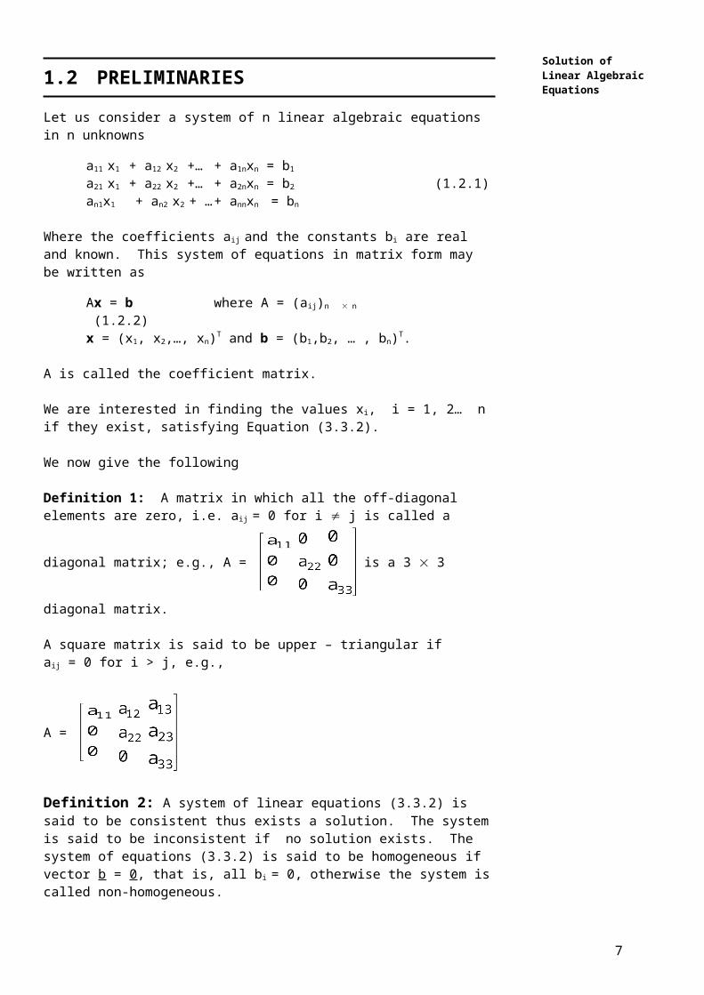
Definition 1: A matrix in which all the off-diagonal elements are zero, i.e. aij = 0 for i

j is called a diagonal matrix; e.g., A = is a 3 3 diagonal matrix.

A square matrix is said to be upper – triangular if aij = 0 for i > j, e.g.,

A =

Definition 2: A system of linear equations (3.3.2) is said to be consistent thus exists a solution. The system is said to be inconsistent if no solution exists. The system of equations (3.3.2) is said to be homogeneous if vector b = 0, that is, all bi = 0, otherwise the system is called non-homogeneous.

We state the following useful result on the solvability of linear systems.

6

Solution of Linear Algebraic EquationsTheorem 1: A non-homogeneous system of n linear equations in n unknown has a

unique solution if and only if the coefficient matrix A is non singular (det A 0) and the solution can be expressed as x = A-1b.

1.3 DIRECT METHODS

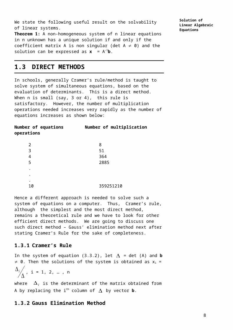
In schools, generally Cramer’s rule/method is taught to solve system of simultaneous equations, based on the evaluation of determinants. This is a direct method. When n is small (say, 3 or 4), this rule is satisfactory. However, the number of multiplication operations needed increases very rapidly as the number of equations increases as shown below:

Number of equations Number of multiplication operations

2 83 514 3645 2885... 10 359251210

Hence a different approach is needed to solve such a system of equations on a computer. Thus, Cramer’s rule, although the simplest and the most direct method, remains a theoretical rule and we have to look for other efficient direct methods. We are going to discuss one such direct method – Gauss’ elimination method next after stating Cramer’s Rule for the sake of completeness.

1.3.1 Cramer’s Rule

In the system of equation (3.3.2), let = det (A) and b 0. Then the solutions of the

system is obtained as xi = , i = 1, 2, … , n

where is the determinant of the matrix obtained from A by replacing the ith column of by vector b.

1.3.2 Gauss Elimination Method

In Gauss’s elimination method, one usually finds successively a finite number of linear systems equivalent to the given one such that the final system is so simple that its solution may be readily computed. In this method, the matrix A is reduced to the form U (upper triangular matrix) by using the elementary row operations like

(i) interchanging any two rows(ii) multiplying (or dividing) any row by a non-zero constant(iii) adding (or subtracting) a constant multiple of one row to another row.

If any matrix A is transformed to another matrix B by a series of row operations, we say that A and B are equivalent matrices. More specifically we have.

Definition 3: A matrix B is said to be row-equivalent to a matrix A, if B can be obtained from A by a using a finite number of row operations. Two linear systems Ax = b and A'x = b' are said to be equivalent if they have the same solution. Hence, if a sequence of elementary operations on Ax = b produces the new system A'x = b', then the systems Ax = b and A'x = b' are equivalent.

7

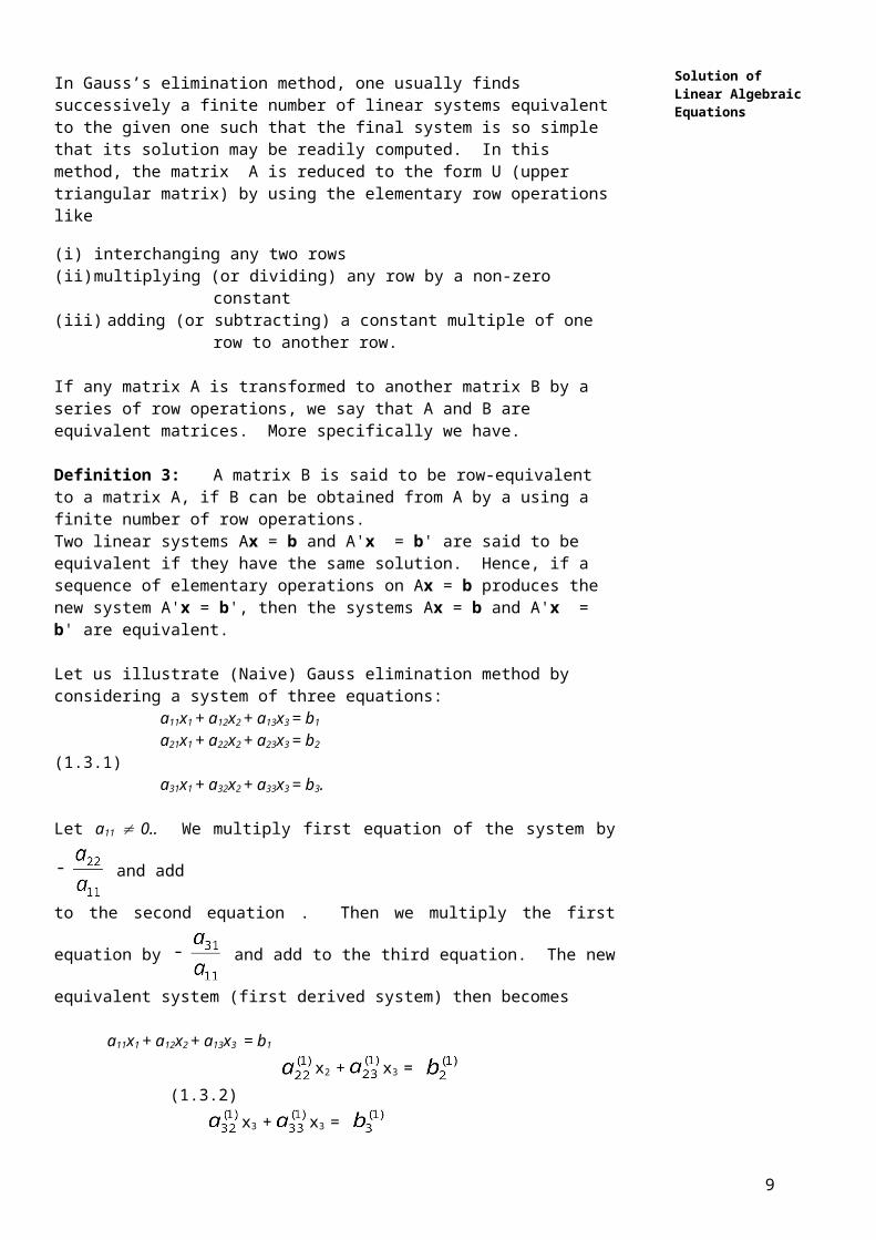
Solution of Linear Algebraic EquationsLet us illustrate (Naive) Gauss elimination method by considering a system of three

equations:a11x1 + a12x2 + a13x3 = b1

a21x1 + a22x2 + a23x3 = b2 (1.3.1)a31x1 + a32x2 + a33x3 = b3.

Let a11 0.. We multiply first equation of the system by and add

to the second equation . Then we multiply the first equation by and add to the

third equation. The new equivalent system (first derived system) then becomes

a11x1 + a12x2 + a13x3 = b1

x2 + x3 = (1.3.2)

x3 + x3 =

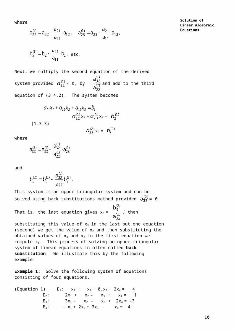
where

etc.

Next, we multiply the second equation of the derived system provided 0, by

and add to the third equation of (3.4.2). The system becomes

x2 + x3 = (1.3.3)

x3 = where

and

This system is an upper-triangular system and can be solved using back substitutions

method provided 0. That is, the last equation gives x3 = then substituting

this value of x3 in the last but one equation (second) we get the value of x2 and then substituting the obtained values of x3 and x2 in the first equation we compute x1. This process of solving an upper-triangular system of linear equations in often called back substitution. We illustrate this by the following example:

Example 1: Solve the following system of equations consisting of four equations.

(Equation 1) E1: x1 + x2 + 0.x3 + 3x4 = 4E2: 2x1 + x2 – x3 + x4 = 1

8

Solution of Linear Algebraic EquationsE3: 3x1 – x2 – x3 + 2x4 = –3

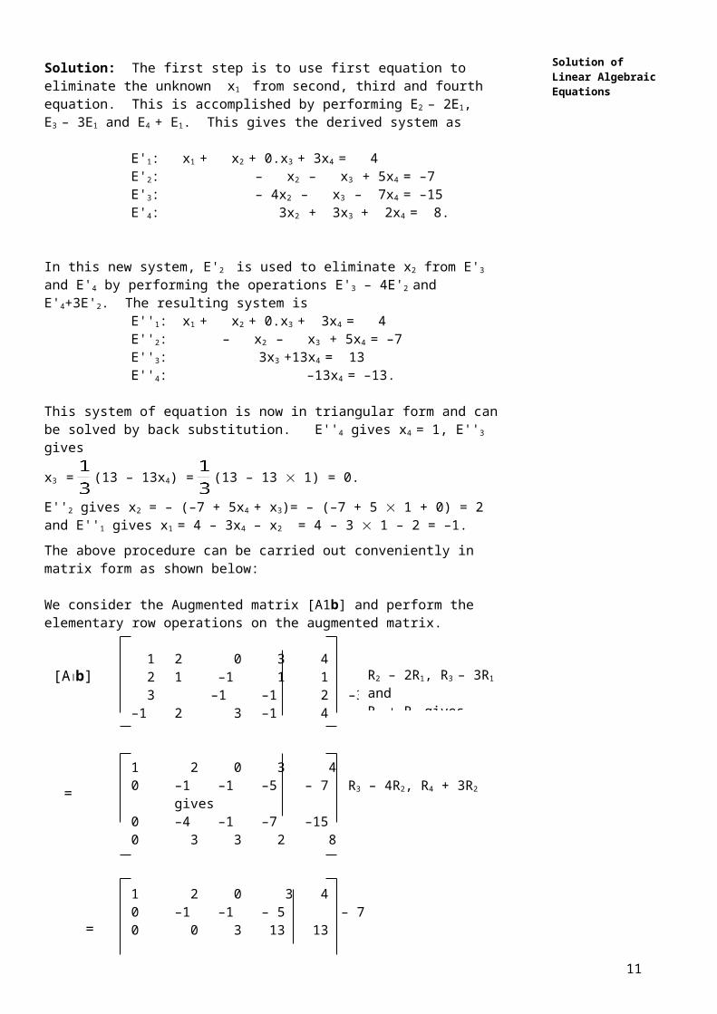
E4: – x1 + 2x2 + 3x3 – x4 = 4.Solution: The first step is to use first equation to eliminate the unknown x1 from second, third and fourth equation. This is accomplished by performing E2 – 2E1, E3 – 3E1 and E4 + E1. This gives the derived system as

E'1: x1 + x2 + 0.x3 + 3x4 = 4E'2: – x2 – x3 + 5x4 = –7E'3: – 4x2 – x3 – 7x4 = –15 E'4: 3x2 + 3x3 + 2x4 = 8.

In this new system, E'2 is used to eliminate x2 from E'3 and E'4 by performing the operations E'3 – 4E'2 and E'4+3E'2. The resulting system is

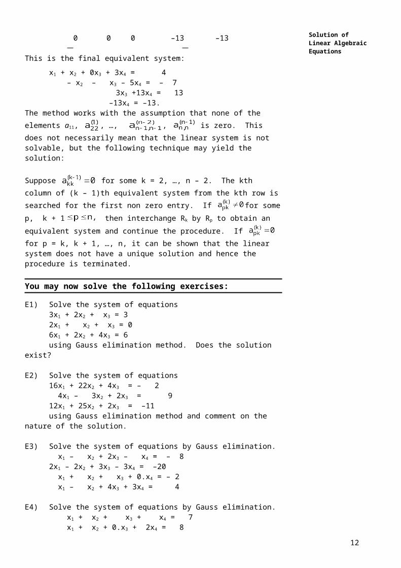
E''1: x1 + x2 + 0.x3 + 3x4 = 4 E''2: – x2 – x3 + 5x4 = –7E''3: 3x3 +13x4 = 13 E''4: –13x4 = –13.

This system of equation is now in triangular form and can be solved by back substitution. E''4 gives x4 = 1, E''3 gives

x3 = (13 – 13x4) = (13 – 13 1) = 0.

E''2 gives x2 = – (–7 + 5x4 + x3)= – (–7 + 5 1 + 0) = 2 and E''1 gives x1 = 4 – 3x4 – x2 = 4 – 3 1 – 2 = –1.

The above procedure can be carried out conveniently in matrix form as shown below:

We consider the Augmented matrix [A1b] and perform the elementary row operations on the augmented matrix.

1 2 0 3 4 2 1 –1 1 1 3 –1 –1 2 –3–1 2 3 –1 4

1 2 0 3 40 –1 –1 –5 – 7 R3 – 4R2, R4 + 3R2 gives0 –4 –1 –7 –150 3 3 2 8

1 2 0 3 40 –1 –1 – 5 – 70 0 3 13 130 0 0 –13 –13

This is the final equivalent system:

x1 + x2 + 0x3 + 3x4 = 4 – x2 – x3 – 5x4 = – 7 3x3 +13x4 = 13

–13x4 = –13.The method works with the assumption that none of the elements a11, , …,

, is zero. This does not necessarily mean that the linear system is not solvable, but the following technique may yield the solution:

9

R2 – 2R1, R3 – 3R1 and R4 + R1 gives

[Ab]

=

=

Solution of Linear Algebraic EquationsSuppose for some k = 2, …, n – 2. The kth column of (k – 1)th equivalent

system from the kth row is searched for the first non zero entry. If for some p, k + 1 then interchange Rk by Rp to obtain an equivalent system and continue the procedure. If for p = k, k + 1, …, n, it can be shown that the linear system does not have a unique solution and hence the procedure is terminated.

You may now solve the following exercises:

E1) Solve the system of equations3x1 + 2x2 + x3 = 32x1 + x2 + x3 = 06x1 + 2x2 + 4x3 = 6using Gauss elimination method. Does the solution exist?

E2) Solve the system of equations16x1 + 22x2 + 4x3 = – 2 4x1 – 3x2 + 2x3 = 912x1 + 25x2 + 2x3 = –11using Gauss elimination method and comment on the nature of the solution.

E3) Solve the system of equations by Gauss elimination. x1 – x2 + 2x3 – x4 = – 82x1 – 2x2 + 3x3 – 3x4 = –20 x1 + x2 + x3 + 0.x4 = – 2 x1 – x2 + 4x3 + 3x4 = 4

E4) Solve the system of equations by Gauss elimination. x1 + x2 + x3 + x4 = 7 x1 + x2 + 0.x3 + 2x4 = 8 2x1 +2x2 + 3x3 + 0.x4 = 10– x1 – x2 – 2x3 + 2x4 = 0

E5) Solve the system of equation by Gauss elimination. x1 + x2 + x3 + x4 = 7 x1 + x2 +2x4 = 5 2x1 + 2x2 + 3x3 = 10– x1 – x2 – 2x3 +2x4 = 0

It can be shown that in Gauss elimination procedure and back substitution

multiplications/divisions and

additions/subtractions are performed respectively. The total arithmetic operation

involved in this method of solving a n n linear system is

multiplication/divisions and additions/subtractions.

Definition 4: In Gauss elimination procedure, the diagonal elements , which have been used as divisors are called pivots and the corresponding equations, are called pivotal equations.

1.3.3 Pivoting Strategies

If at any stage of the Gauss elimination, one of these pivots say , vanishes then we have indicated a modified procedure. But it may also happen that

10

Solution of Linear Algebraic Equationsthe pivot though not zero, may be very small in magnitude compared to the

remaining elements ( i) in the ith column. Using a small number as divisor may lead to growth of the round-off error. The use of large multipliers like

etc. will lend to magnification of errors both during the elimination phase and during the back substitution phase of the solution procedure. This can be avoided by rearranging the remaining rows (from ith row up to nth row) so as to obtain a non-vanishing pivot or to choose one that is largest in magnitude in that column. This is called pivoting strategy.

There are two types of pivoting strategies: partial pivoting (maximal column pivoting) and complete pivoting. We shall confine to simple partial pivoting and complete pivoting. That is, the method of scaled partial pivoting will not be discussed. Also there is a convenient way of carrying out the pivoting procedure where instead of interchanging the equations all the time, the n original equations and the various changes made in them can be recorded in a systematic way using the augmented matrix [A1b] and storing the multiplies and maintaining pivotal vector. We shall just illustrate this with the help of an example. However, leaving aside the complexities of notations, the procedure is useful in computation of the solution of a linear system of equations.

If exact arithmetic is used throughout the computation, pivoting is not necessary unless the pivot vanishes. But, if computation is carried up to a fixed number of digits (precision fixed), we get accurate results if pivoting is used.

The following example illustrates the effect of round-off error while performing Gauss elimination:

Example 2: Solve by the Gauss elimination the following system using four-digit arithmetic with rounding.

0.003000x1 + 59.14 x2 = 59.17 5.291x1 – 6.130x2 = 46.78.

Solution: The first pivot element = a11 = 0.0030 and its associated multiplier is

Performing the operation of elimination of x1 from the second equation with appropriate rounding we got

0.003000 x1 + 59.14x2 = 59.17 – 104300 x2 = –104400

By backward substitution we have

x2 = 1.001 and x1 =

The linear system has the exact solution x1 = 10.00 and x2= 1,000.

11

Solution of Linear Algebraic EquationsHowever, if we use the second equation as the first pivotal equation and solve the

system, the four digit arithmetic with rounding yields solution as x1=10.00 and x2 = 1.000. This brings out the importance of partial or maximal column pivoting.Partial pivoting (Column Pivoting)

In the first stage of elimination, instead of using a11 0 as the pivot element, the first column of the matrix A ([A1b]) is searched for the largest element in magnitude and this largest element is then brought at the position of the first pivot by interchanging first row with the row having the largest element in magnitude in the first column.

Next, after elimination of x1, the second column of the derived system is searched for the largest element in magnitude among the (n – 1) element leaving the first element. Then this largest element in magnitude is brought at the position of the second pivot by interchanging the second row with the row having the largest element in the second column of the derived system. The process of searching and interchanging is repeated in all the (n – 1) stages of elimination. For selecting the pivot we have the following algorithm:

For i = 1, 2, …, n find j such that

Interchange ith and jth rows and eliminate xi.

Complete Pivoting

In the first stage of elimination, we look for the largest element in magnitude in the entire matrix A first. If the element is apq, then we interchange first row with pth row and interchange first column with qth column, so that apq can be used as a first pivot. After eliminating xq, the process is repeated in the derived system, more specifically in the square matrix of order n – 1, leaving the first row and first column. Obviously, complete pivoting is quite cumbersome.

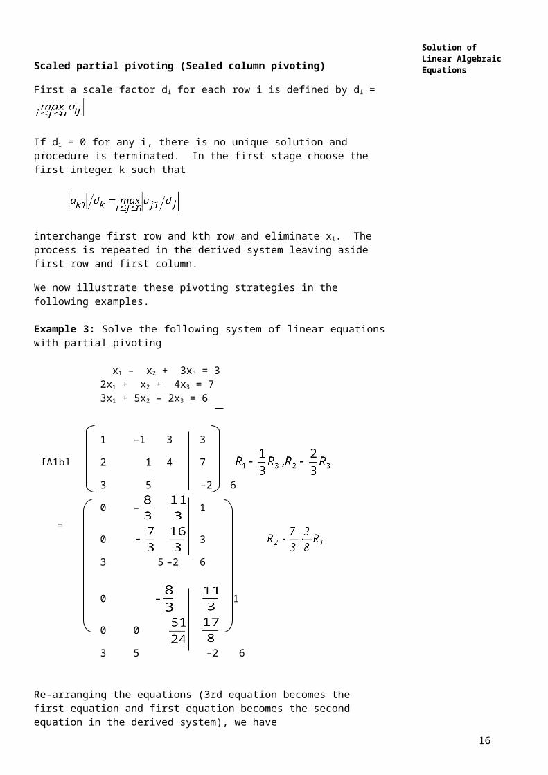
Scaled partial pivoting (Sealed column pivoting)

First a scale factor di for each row i is defined by di =

If di = 0 for any i, there is no unique solution and procedure is terminated. In the first stage choose the first integer k such that

interchange first row and kth row and eliminate x1. The process is repeated in the derived system leaving aside first row and first column.

We now illustrate these pivoting strategies in the following examples.

Example 3: Solve the following system of linear equations with partial pivoting

x1 – x2 + 3x3 = 32x1 + x2 + 4x3 = 73x1 + 5x2 – 2x3 = 6

1 –1 3 3

2 1 4 7

12

[A1b]=

Solution of Linear Algebraic Equations3 5 –2 6

0 – 1

0 3

3 5 –2 6

0 – 1

0 0

3 5 –2 6

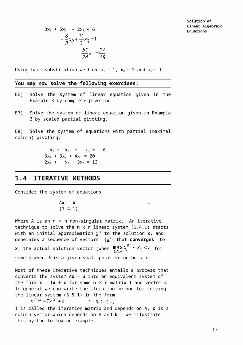
Re-arranging the equations (3rd equation becomes the first equation and first equation becomes the second equation in the derived system), we have

3x1 + 5x2 – 2x3 = 6

Using back substitution we have x1 = 1, x2 = 1 and x3 = 1.

You may now solve the following exercises:

E6) Solve the system of linear equation given in the Example 3 by complete pivoting.

E7) Solve the system of linear equation given in Example 3 by scaled partial pivoting.

E8) Solve the system of equations with partial (maximal column) pivoting.

x1 + x2 + x3 = 63x1 + 3x2 + 4x3 = 202x1 + x2 + 3x3 = 13

1.4 ITERATIVE METHODS

Consider the system of equations

Ax = b … (1.4.1) Where A is an n n non-singular matrix. An iterative technique to solve the n x n linear system (1.4.1) starts with an initial approximation x(0) to the solution x, and generates a sequence of vectors {xk that converges to x, the actual solution vector

(When for some k when is a given small positive numbers.).

Most of these iterative techniques entails a process that converts the system Ax = b into an equivalent system of the form x = Tx + c for some n n matrix T and vector c. In general we can write the iteration method for solving the linear system (3.5.1) in the form

k = 0, 1, 2, …,

13

=

Solution of Linear Algebraic EquationsT is called the iteration matrix and depends on A, c is a column vector which depends

on A and b. We illustrate this by the following example.

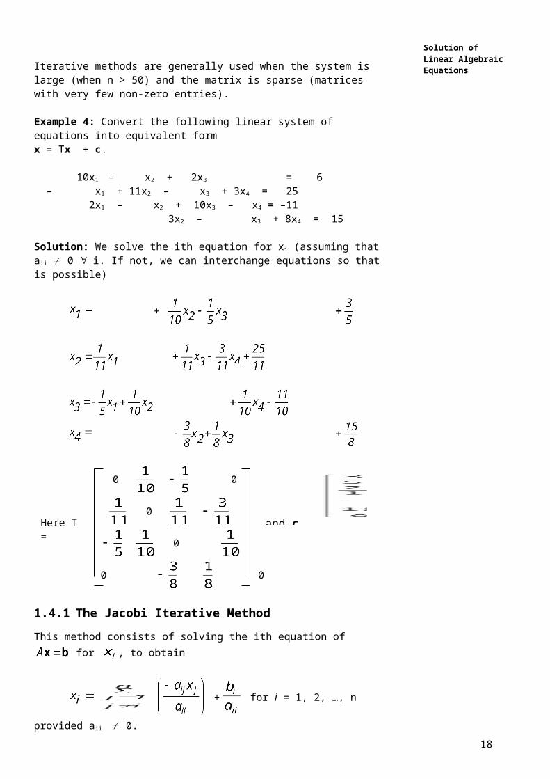
Iterative methods are generally used when the system is large (when n > 50) and the matrix is sparse (matrices with very few non-zero entries).

Example 4: Convert the following linear system of equations into equivalent form x = Tx + c.

10x1 – x2 + 2x3 = 6 – x1 + 11x2 – x3 + 3x4 = 25 2x1 – x2 + 10x3 – x4 = –11 3x2 – x3 + 8x4 = 15

Solution: We solve the ith equation for xi (assuming that aii 0 i. If not, we can interchange equations so that is possible)

+

0 0

0

0

0 0

1.4.1 The Jacobi Iterative Method

This method consists of solving the ith equation of for , to obtain

+ for i = 1, 2, …, n

provided aii 0.

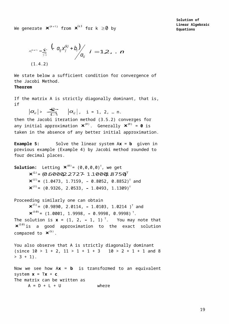
We generate from for k by

(1.4.2)

We state below a sufficient condition for convergence of the Jacobi Method.Theorem

14

and c =Here T =

Solution of Linear Algebraic EquationsIf the matrix A is strictly diagonally dominant, that is, if

> , i = 1, 2, … n.

then the Jacobi iteration method (3.5.2) converges for any initial approximation . Generally = 0 is taken in the absence of any better initial approximation.

Example 5: Solve the linear system Ax = b given in previous example (Example 4) by Jacobi method rounded to four decimal places.

Solution: Letting = (0,0,0,0)T, we get == (1.0473, 1.7159, – 0.8052, 0.8852)T and= (0.9326, 2.0533, – 1.0493, 1.1309)T

Proceeding similarly one can obtain= (0.9890, 2.0114, – 1.0103, 1.0214 )T and= (1.0001, 1.9998, – 0.9998, 0.9998) T.

The solution is x = (1, 2, – 1, 1) T. You may note that is a good approximation to the exact solution compared to .

You also observe that A is strictly diagonally dominant (since 10 > 1 + 2, 11 > 1 + 1 + 3 10 > 2 + 1 + 1 and 8 > 3 + 1).

Now we see how Ax = b is transformed to an equivalent system x = Tx + c.

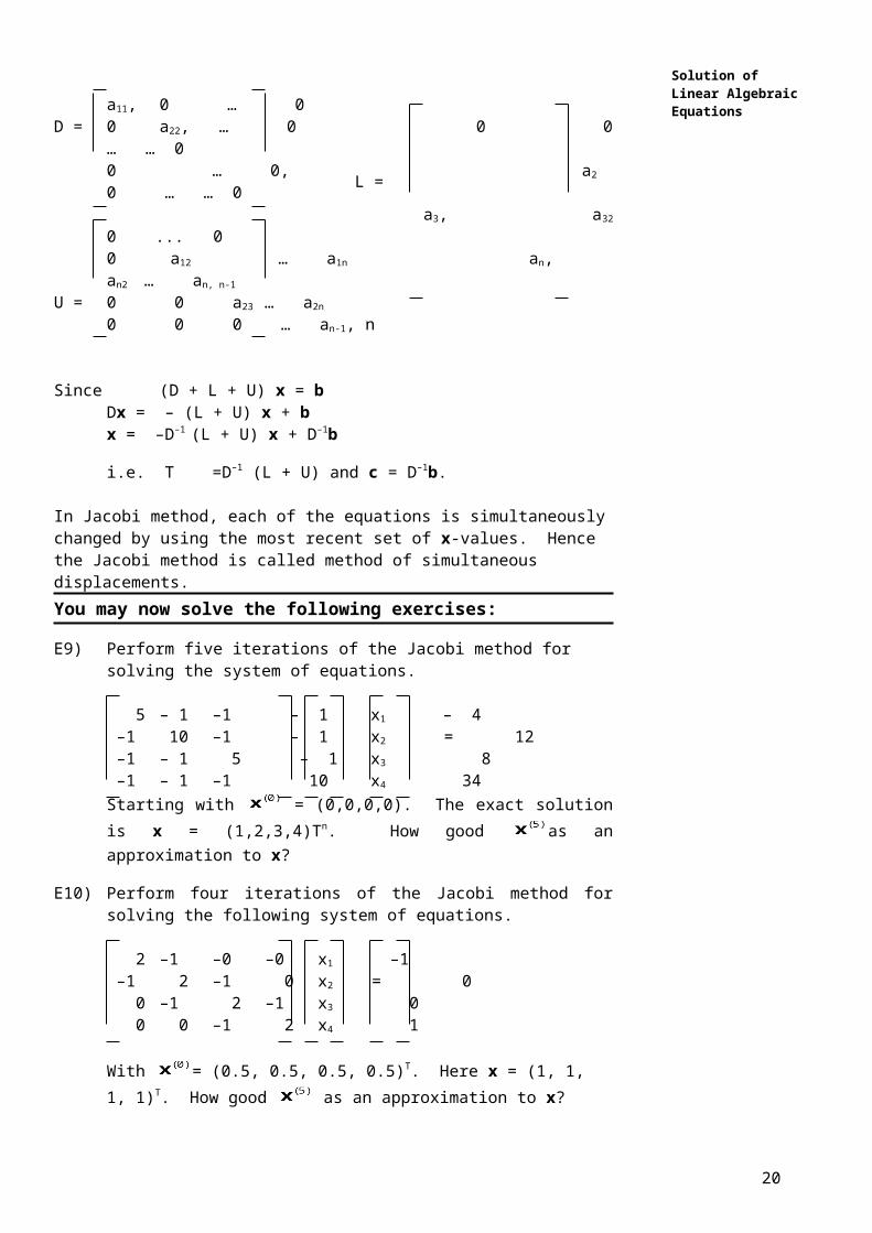
The matrix can be written asA = D + L + U where

a11, 0 … 0D = 0 a22, … 0 0 0 … … 0

0 … 0, ann a2 0 … … 0a3, a32 0 ... 0

0 a12 … a1n an, an2 … an, n-1

U = 0 0 a23 … a2n

0 0 0 … an-1, n

Since (D + L + U) x = bDx = – (L + U) x + b

x = –D–1 (L + U) x + D–1b

i.e. T =D–1 (L + U) and c = D–1b.

In Jacobi method, each of the equations is simultaneously changed by using the most recent set of x-values. Hence the Jacobi method is called method of simultaneous displacements.You may now solve the following exercises:

E9) Perform five iterations of the Jacobi method for solving the system of equations.

5 – 1 –1 – 1 x1 – 4 –1 10 –1 – 1 x2 = 12 –1 – 1 5 – 1 x3 8 –1 – 1 –1 10 x4 34

15

L =

Solution of Linear Algebraic EquationsStarting with = (0,0,0,0). The exact solution is x = (1,2,3,4)Tn. How

good as an approximation to x?

E10) Perform four iterations of the Jacobi method for solving the following system of equations.

2 –1 –0 –0 x1 –1 –1 2 –1 0 x2 = 0 0 –1 2 –1 x3 0 0 0 –1 2 x4 1

With = (0.5, 0.5, 0.5, 0.5)T. Here x = (1, 1, 1, 1)T. How good as an approximation to x?

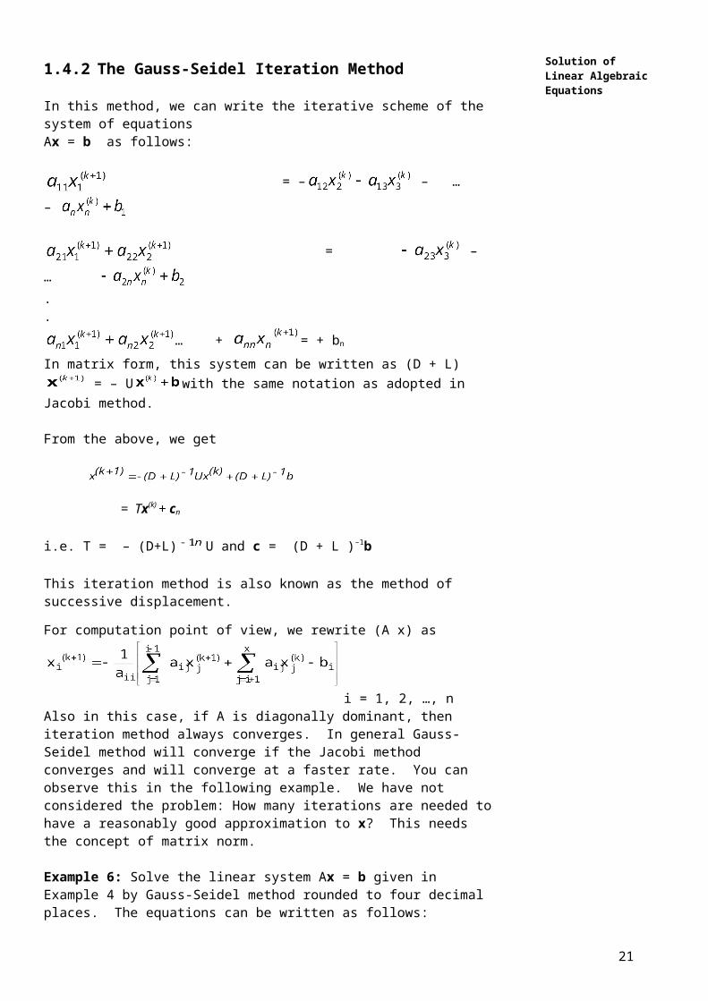
1.4.2 The Gauss-Seidel Iteration Method

In this method, we can write the iterative scheme of the system of equationsAx = b as follows:

= – – … –

= – … ..

…+ = + bn

In matrix form, this system can be written as (D + L) = – U with the same notation as adopted in Jacobi method.

From the above, we get

= Tx(k) + cn

i.e. T = – (D+L) U and c = (D + L )–1b

This iteration method is also known as the method of successive displacement.

For computation point of view, we rewrite (A x) as

i = 1, 2, …, nAlso in this case, if A is diagonally dominant, then iteration method always converges. In general Gauss-Seidel method will converge if the Jacobi method converges and will converge at a faster rate. You can observe this in the following example. We have not considered the problem: How many iterations are needed to have a reasonably good approximation to x? This needs the concept of matrix norm.

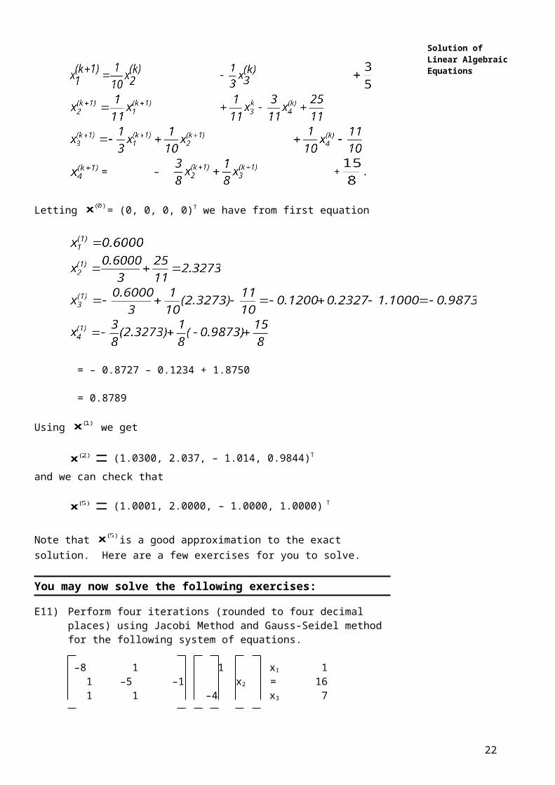
Example 6: Solve the linear system Ax = b given in Example 4 by Gauss-Seidel method rounded to four decimal places. The equations can be written as follows:

16

Solution of Linear Algebraic Equations

= – + .

Letting = (0, 0, 0, 0)T we have from first equation

= – 0.8727 – 0.1234 + 1.8750

= 0.8789

Using we get

(1.0300, 2.037, – 1.014, 0.9844)T and we can check that

(1.0001, 2.0000, – 1.0000, 1.0000) T

Note that is a good approximation to the exact solution. Here are a few exercises for you to solve.

You may now solve the following exercises:

E11) Perform four iterations (rounded to four decimal places) using Jacobi Method and Gauss-Seidel method for the following system of equations.

–8 1 1 x1 1 1 –5 –1 x2 = 16 1 1 –4 x3 7

With = (0, 0, 0)T. The exact solution is (–1, –4, –3)T. Which method gives better approximation to the exact solution?

E12) For linear system given in E10), use the Gauss Seidel method for solving the system starting with = (0.5, 0.5, 0.5, 0.5)T obtain by Gauss-Seidel method and compare this with obtained by Jacobi method in E10).

1.4.3 Comparison of Direct and Iterative Methods

Both the methods have their strengths and weaknesses and a choice is based on the particular linear system to be solved. We mention a few of these below:

17

Solution of Linear Algebraic EquationsDirect Method

1. The direct methods are generally used when the matrix A is dense or filled, that is, there are few zero elements, and the order of the matrix is not very large, say n < 50.

2. The rounding errors may become quite large for ill conditioned equations (If at any stage during the application of pivoting strategy, it is found that all values of for m = k + 1, to n are less than a pre-assigned small quantity , then the equations are ill-conditioned and no useful solution is obtained). Ill-conditioned matrices are not discussed in this unit.

Iterative Method

1. These methods are generally used when the matrix A is sparse and the order of the matrix A is very large say n > 50. Sparse matrices have very few non-zero elements.

2. An important advantage of the iterative methods is the small rounding error. Thus, these methods are good choice for ill-conditioned systems.

3. However, convergence may be guaranteed only under special conditions. But when convergence is assured, this method is better than direct.

With this we conclude this unit. Let us now recollect the main points discussed in this unit.

1.5 SUMMARY

In this unit we have dealt with the following:

1. We have discussed the direct methods and the iterative techniques for solving linear system of equations Ax = b where A is an n n, non-singular matrix.

2. The direct methods produce the exact solution in a finite number of steps provided there are no round off errors. Direct method is used for linear system Ax = b where the matrix A is dense and order of the matrix is less than 50.

3. In direct methods, we have discussed Gauss elimination, and Gauss elimination with partial (maximal column) pivoting and complete or total pivoting.

4. We have discussed two iterative methods, Jacobi method and Gauss-Seidel method and stated the convergence criterion for the iteration scheme. The iterative methods are suitable for solving linear systems when the matrix is sparse and the order of the matrix is greater than 50.

1.6 SOLUTION/ANSWERS

E1) 3 2 1 3 2 1 –1 0 6 2 4 6

3 2 1 3

18

[A1b]

Solution of Linear Algebraic Equations 0 – – 2

0 –2 2 0

3 2 1 3

0 – – – 2

0 0 0 12

This system has no solution since x3 cannot be determined from the last equation. This system is said to be inconsistent. Also note that del (A) = 0.

E2) 16 22 4 – 2 4 – 3 2 9 12 25 2 – 11

16 22 4 2

0 – 1

0 –1 –

16 22 4 2

0 – 1

0 0 0 0

and x3 = (–2 – 22x3 – 22x3)

This system has infinitely many solutions. Also you may check that det (A) = 0.

E3) Final derived system:

1 –1 2 –1 –8 0 2 –1 1 6 and the solution is x4 = 2, x3 = 2 0 0 –1 –1 –4 x2 = 3, x1 = –7. 0 0 0 2 4

E4) Final derived system:

1 –1 1 1 7 0 0 –1 1 1 0 0 1 –2 –4 and the solution is 0 0 0 1 3

x4 = 3, x3 = 2 , x2 arbitrary and x1 = 2 – x2.

Thus this linear system has infinite number of solutions.

E5) Final derived system:

1 1 1 1 7 0 0 –1 1 –2 0 0 1 –2 –4 and the solution does not

19

[A1b]

x3 = arbitrary value, x2 =

Solution of Linear Algebraic Equations 0 0 0 1 3

exist since we have x4 = 3, x3 = 2 and third equation –x3 + x4 = –2 implies 1 = –2, leading to a contradiction.

E6) Since |a32| is maximum we rewrite the system as

5 3 –2 6 by interchanging R1 and R3 and C1 and C2

1 2 4 7 R2 –

gives –1 1 3 3

5 3 –2 6 5 –2 3 6

0 0

0 0

Since |a23| is maximum –

By R3 R2 we have

5 –2 3 6

0

0 0

We have x2 = 1,

3x1 = 6 – 5 + 2 x1 = 1

E7) For solving the linear system by sealed partial pivoting we note that d1 = 3, d2

= 4 and d3 = 5 in

1 –1 3 32 1 4 7 p = [a, 2, 3]T

3 5 –2 6

Since max , third equation is chosen as the first pivotal equation.

Eliminating x1 we haved

3 1

20

by inter-changing C2 and C3

W= [A1b] =

W1=where we have used a square to enclose the pivot element and

Solution of Linear Algebraic Equations4 – 3

5 3 5 –2 6

in place of zero entries, after elimination of x1 from 1st and 2nd equation, we have

stored the multipliers. Here m11 =

Instead of interchanging rows (here R1 and R3)we keep track of the pivotal equations being used by the vector p=[3,2,1]T

In the next step we consider max

So the second pivotal equation is the first equation.

i.e. p = [3, 1, 3]T and multiplier is

1

p = [3, 1, 2]T

3 5 –2 6

The triangular system is as follows:

= 6

By back substitution, this yields x1 = 1, x2 = 1 and x3 = 1.

Remark: The p vector and storing of multipliers help solving the system Ax = b' where b is changed b'.

E8) 1 1 1 6 3 3 4 203 3 4 20 1 1 1 62 1 3 13 2 1 3 13

3 3 4 20 13 3 4 20

0 0 – – 0 –1 –

0 –1 – 0 0 – –

Since the resultant matrix is in triangular form, using back substitution we get x3 = 2, x2 = 1 and x1 = 3.

E9) Using [0, 0, 0, 0]T we have

[–0.8, 1.2, 1.6, 3.4]T

[0.44, 1.62, 2.36, 3.6]T

[0.716,1.84, 2.732, 3.842]T

[0.8823, 1.9290, 2.8796, 3.9288]T

21

[A, b]=

and W(2)=

Solution of Linear Algebraic Equations

E10) Using [0.5, 0.5, 0.5, 0.5]T, we have

[0.75, 0.5, 0.5, 0.75]T

[0.75,0.625,0.625,0.75]T

[0.8125, 0.6875, 0.6875, 0.8125]T

[0.8438, 0.75, 0.75, 0.8438]T

E 11) By Jacobi method we have [–0.125, –3.2, –1.75]T

[–0.7438, –3.5750, –2.5813]T

[–0.8945, –3.8650, –2.8297]T

[–0.9618, –3.9448, –2.9399]

Where as by Gauss-Seidel method, we have [–0.125, –3.225, –2.5875]T

[–0.8516, –3.8878,–2.9349]T

[–0.9778, –3.9825, –2.9901]T

[–0.9966, –3.9973, –2.9985]T

E12) Starting with the initial approximation[0.5, 0.5, 0.5, 0.5]T, we have the following iterates:

[0.75, 0.625,0.5625,0.7813]T

[0.8125, 0.6875, 0.7344, 0.8672]T

[0.8438, 0.7891, 0.8282, 0.9141]T

[0.8946, 0.8614, 0.8878, 0.9439]T

Since the exact solution is x = [1, 1, 1, 1]T, the Gauss, Seidel method gives better approximation than the Jacobi method at fourth iteration.

22