IFRS and European Commercial Banks: Value Relevance and ...

1

UNIVERSITY OF BIRMINGHAM BIRMINGHAM BUSINESS SCHOOL

IFRS and European Commercial Banks: Value Relevance

and Economic Consequences

A thesis submitted to the University of Birmingham, UK

for the degree of Doctor of Philosophy

July 2011

Athanasios A. Dimos

University of Birmingham Research Archive

e-theses repository This unpublished thesis/dissertation is copyright of the author and/or third parties. The intellectual property rights of the author or third parties in respect of this work are as defined by The Copyright Designs and Patents Act 1988 or as modified by any successor legislation. Any use made of information contained in this thesis/dissertation must be in accordance with that legislation and must be properly acknowledged. Further distribution or reproduction in any format is prohibited without the permission of the copyright holder.

2

Abstract

2005 was a landmark year in the European Union’s (EU) financial reporting history as all EU

listed firms were required to switch from national accounting standards to IFRS. Using a sample

of European commercial banks, this study explores two research questions within the framework

of equity valuation theory: (i) whether the disclosed fair value estimates of loans and advances;

held-to-maturity investments; deposits; and other debt, as well as the recognition of derivatives at

fair value, are value relevant, (ii) whether the adoption of IFRS led to a reduction in European

banks’ cost of equity capital.

The results show that the fair value of loans and advances and other debt are value relevant as is

the recognition of derivatives at fair value. Further analysis revealed that the relevance of fair

value of loans and derivatives is contingent on banks’ financial health and earnings variability,

respectively, as well as on the ability of countries to enforce IFRS. The findings also indicate that

the cost of equity capital of European commercial banks decreased after the adoption of IFRS.

However, banks domiciled in countries with continental accounting standards and weak

enforcement rules experienced a greater reduction in their cost of equity capital.

3

Acknowledgements

I am very grateful to my supervisors, Professor Rowan Jones and Dr. George Georgiou who

took a keen interest in the work and provided detailed feedback. I would also like to thank the

State Scholarships Foundation (I.K.Y.) for providing me with a scholarship to perform

postgraduate studies in the field of financial accounting. Its financial support was crucial for the

completion of this thesis.

Finally, I would like to thank my parents, Antonios and Kyratso Dimos for their guidance,

support, and encouragement throughout my life – I therefore dedicate this thesis to them.

4

Table of Contents

Abbreviations ................................................................................................................................ 11

Chapter 1: Introduction ................................................................................................................. 12

1.1 Introduction ........................................................................................................................ 12

1.2 Research objectives ............................................................................................................ 14

1.3 Overview of methodology .................................................................................................. 17

1.3.1 Theoretical framework ................................................................................................ 17

1.3.2 Research Methodology ............................................................................................... 18

1.4 Contribution to the literature .............................................................................................. 20

1.5 Structure of the thesis ......................................................................................................... 22

1.6 Conclusion .......................................................................................................................... 24

Chapter 2: Regulations for European Commercial Banks ............................................................ 25

2.1 Introduction ........................................................................................................................ 25

2.2 Accounting for financial instruments ................................................................................. 26

2.2.1 Classification of financial instruments ....................................................................... 27

2.2.2 Measurement and presentation issues ......................................................................... 28

2.2.3 Hedge accounting ....................................................................................................... 32

2.2.4 EU on the adoption of IFRS ....................................................................................... 34

2.2.5 A new standard on financial instruments (IFRS 9) .................................................... 37

2.2.6 US GAAP on financial instruments ............................................................................ 39

2.3 Capital regulations for commercial banks .......................................................................... 42

2.3.1 The need for regulation ............................................................................................... 42

5

2.3.2 The 1988 Capital Accord (Basel I) ............................................................................. 42

2.3.3 Basel Amendments (1996) to incorporate market risk ............................................... 44

2.3.4 Basel II – The Three Pillar Approach ......................................................................... 45

2.3.5 EU on Capital Adequacy Requirements ..................................................................... 47

2.4 Conclusion .......................................................................................................................... 48

Chapter 3: Theoretical Framework ............................................................................................... 49

3.1 Introduction ........................................................................................................................ 49

3.2 Equity valuation theory ...................................................................................................... 50

3.2.1 Equity valuation models ............................................................................................. 50

3.2.1.1 The Dividend Discount Model (DDM) ................................................................... 50

3.2.1.2 The Residual Income Valuation Model (RIVM) ..................................................... 52

3.2.1.3 The Ohlson (1995) model ........................................................................................ 55

3.2.1.4 The Feltham & Ohlson (1995) model ...................................................................... 58

3.2.1.5 The Earnings Growth Model (EGM) - Ohlson & Juettner (2005) Model ............... 61

3.2.1.6 The Balance Sheet Model (BSM) ............................................................................ 63

3.2.2 Cost of equity capital .................................................................................................. 66

3.3 CE and accounting standards .............................................................................................. 69

3.3.1 Increased disclosure and CE ....................................................................................... 69

3.3.2 Uniformity of accounting standards and CE ............................................................... 74

3.4 A critical view of value relevance research ........................................................................ 76

3.5 Conclusion .......................................................................................................................... 78

6

Chapter 4: Review of Value Relevance Empirical Studies ........................................................... 81

4.1 Introduction ........................................................................................................................ 81

4.2 Empirical Studies on Banks ................................................................................................ 82

4.2.1 The US literature ......................................................................................................... 82

4.2.1.1 Evidence before SFAS No. 107 ............................................................................... 83

4.2.1.2 Evidence under SFAS No. 107, 109, and 133 ......................................................... 85

4.2.1.3 Evidence under SFAS No. 115 ................................................................................ 92

4.2.1.4 Evidence under SFAS No. 157 ................................................................................ 94

4.2.2 The non-US literature ................................................................................................. 95

4.3 Empirical studies on Non-Banks ........................................................................................ 99

4.3.1 US – Empirical Studies ............................................................................................... 99

4.3.1.1 Financial instruments ............................................................................................... 99

4.3.1.2 Non-financial instruments...................................................................................... 102

4.3.2 Non-US – Empirical Studies .................................................................................... 104

4.4 Conclusion ........................................................................................................................ 109

Chapter 5: Review of the Cost of Equity Empirical Studies ....................................................... 114

5.1 Introduction ...................................................................................................................... 114

5.2 Review of the empirical studies ....................................................................................... 115

5.2.1 The Non-IFRS literature ........................................................................................... 115

5.2.2 The IFRS Literature .................................................................................................. 122

5.2.2.1 Voluntary disclosures of IFRS ............................................................................... 123

7

5.2.2.2 Mandatory disclosures of IFRS ............................................................................. 128

5.3 Conclusion ........................................................................................................................ 138

Chapter 6: Research Methodology on the Value Relevance ....................................................... 141

6.1 Introduction ...................................................................................................................... 141

6.2 Development of Hypotheses ............................................................................................. 142

6.2.1 Fair value disclosures................................................................................................ 142

6.2.2 Recognition of derivatives’ fair values ..................................................................... 145

6.3 Empirical Methodology .................................................................................................... 148

6.3.1 Fair value disclosures................................................................................................ 148

6.3.1.1 Primary model specification .................................................................................. 148

6.3.1.2 Alternative model specification ............................................................................. 162

6.3.2 Recognition of derivatives’ fair values ..................................................................... 165

6.3.2.1 Primary model specification .................................................................................. 165

6.3.2.2 Alternative model specification ............................................................................. 167

6.4 Sample Selection .............................................................................................................. 168

6.5 Conclusion ........................................................................................................................ 172

Chapter 7: Research Methodology on the Cost of Equity Capital .............................................. 175

7.1 Introduction ...................................................................................................................... 175

7.2 Development of Hypotheses ............................................................................................. 176

7.3 Empirical Analysis ........................................................................................................... 179

7.3.1 Estimation of cost of equity ...................................................................................... 179

7.3.1.1 The Gebhardt et al. (2001) method ........................................................................ 179

8

7.3.1.2 The Claus & Thomas (2001) method .................................................................... 181

7.3.1.3 The Gode & Mohanram (2003) method ................................................................ 182

7.3.1.4 The Easton (2004) method ..................................................................................... 183

7.3.2 Primary analysis ........................................................................................................ 184

7.3.3 Additional analysis ................................................................................................... 189

7.3.4 Robustness tests ........................................................................................................ 193

7.4 Sample procedure ............................................................................................................. 194

7.5 Conclusion ........................................................................................................................ 196

Chapter 8: Findings on the value relevance ................................................................................ 198

8.1 Introduction ...................................................................................................................... 198

8.2 Descriptive statistics ......................................................................................................... 198

8.3 Fair value disclosures ....................................................................................................... 203

8.3.1 Results from the primary specification model .......................................................... 203

8.3.2 Results from the alternative specification models .................................................... 210

8.4 Derivatives’ fair value recognitions ................................................................................. 213

8.4.1 Results from the primary specification model .......................................................... 214

8.4.2 Results from the alternative specification models .................................................... 219

8.4.3 The use of hedging derivatives by European banks ................................................. 223

8.5 Conclusion ........................................................................................................................ 226

Chapter 9: Findings on the Cost of Equity Capital ..................................................................... 230

9.1 Introduction ...................................................................................................................... 230

9

9.2 Descriptive statistics ......................................................................................................... 231

9.3 Univariate analysis ........................................................................................................... 238

9.4 Multivariate analysis ........................................................................................................ 245



9.5 Robustness tests ................................................................................................................ 257



9.6 Conclusion ........................................................................................................................ 266

Chapter 10: Synopsis and Conclusion ......................................................................................... 268

10.1 Introduction .................................................................................................................... 268

10.2 Summary of the Chapters 1-7 ......................................................................................... 269

10.3 Main findings .................................................................................................................. 272

10.3.1 Value relevance of fair value disclosures ............................................................... 272

10.3.2 Value relevance of derivatives’ fair value recognition ........................................... 274

10.3.3 Economic consequences ......................................................................................... 274

10.4 Limitations of the study .................................................................................................. 275

10.5 Recommendations for future research ............................................................................ 277

10.6 Conclusion ...................................................................................................................... 278

Appendix A ................................................................................................................................. 281

Appendix B ................................................................................................................................. 288

Appendix C ................................................................................................................................. 294

10

Appendix D ................................................................................................................................. 298

Appendix E .................................................................................................................................. 310

References ................................................................................................................................... 311

11

Abbreviations

AG Application Guidance

BIS Bank for International Settlements

BSM Balance Sheet Model

CAPM Capital Asset Pricing Model

CE Cost of Equity Capital

CSR Clean Surplus Relation

DDM Dividend Discount Model

EBF European Banking Federation

EC European Commission

ECB European Central Bank

EFRAG European Financial Reporting Advisory Group

EGM Earnings Growth Model

EU European Union

FDIC Federal Deposit Insurance Corporation

IAS International Accounting Standards

IASB International Accounting Standards Board

IFRS International Financial Reporting Standards

FASB Financial Accounting Standards Board

RIVM Residual Income Valuation Model

12

Chapter 1: Introduction

1.1 Introduction

This thesis deals with the application of the International Financial Reporting Standards

(hereafter IFRS) by a single industry, the European commercial banking. The study relates to

two major streams of accounting literature, i) the value relevance of fair value accounting, and ii)

the economic consequences from the mandatory adoption of IFRS.

Value relevance research deals with the statistical relationship between the accounting numbers

and measures of market value, such as share prices or returns (Barth, 2000). A major strand of

value relevance studies examines the significance of fair value estimates in explaining share

prices (Landsman, 2007). These studies provide evidence on whether fair values are useful in

making investment decisions. Fair value accounting has been proposed as an alternative

measurement system to historical cost accounting and has been adopted by the International

Accounting Standards Board (hereafter, IASB) and the US standard setting body, the Financial

Accounting Standards Board (hereafter, FASB), in several of their standards. For example, fair

values have been used extensively in measuring financial instruments, such as investment

securities and derivative financial instruments (trading and hedging). The usefulness of fair

values over and above other measurement attributes (e.g. historical costs), in explaining market

values, is another major question of the value relevance research. (Barth, 2006b)

The IASB deals with financial instruments in the accounting standards: International Accounting

Standard (hereafter, IAS) 39, IAS 32, IFRS 7 and IFRS 9. IAS 39 is concerned with the

recognition and the measurement of financial instruments, and IAS 32 and IFRS 7 with their

13

presentation and disclosure, respectively. IFRS 9 is a new standard on financial instruments with

which the IASB intents to replace completely IAS 39. The term fair value is defined in IAS 39 as:

‘the amount for which an asset could be exchanged, or a liability settled, between knowledgeable, willing parties in an arm’s length transaction’ (see, IAS 39, 2003b).

Proponents of fair value accounting argue that fair values provide more relevant and up-to-date

information to investors than historical cost accounting, and thus whenever it is possible assets

and liabilities should be measured at fair value (Penman, 2007, p. 33). However, there are

concerns with respect to the reliability of fair value estimates as sometimes they are based on

subjective assumptions.

The other stream of accounting research that this thesis deals with relates to the economic

consequences of the mandatory adoption of IFRS. IFRS are regarded as a set of high quality

accounting standards as compared to national accounting standards. For example, Barth et al.

(2008) examined the accounting quality of the IFRS in 21 countries and found less earnings

management, more timely loss recognition, and more value relevance as compared to a control

group of firms following non-US national accounting standards. Moreover, the adoption of IFRS

is a commitment to increased disclosure by many countries, such as the risk related information

of all financial instruments (e.g., IFRS 7 requires the disclosure of credit risk, liquidity risk, and

market risk). In theory, high quality accounting standards and increased disclosure are related to

less uncertainty for investors and thus, a reduction in the information asymmetry between

managers and shareholders (Diamond & Verrecchia, 1991). This leads to a reduction in the cost

of equity capital (hereafter CE). The adoption of IFRS can also reduce the CE through the

information comparability across the financial statements of firms as investors (and analyst) do

14

not have to adjust financial accounts to overcome the differences between national accounting

standards.

1.2 Research objectives

Previous studies support the view that fair values of financial instruments are relevant and

reliable enough to be reflected in share prices (Barth, 1994; Barth et al., 1996; Venkatachalam,

1996; Ahmed et al., 2006). However, most of these studies deal with US GAAP and US

commercial banks. To date there is not a single study that tests the value relevance of fair values

of European banks that report under the new adopted IFRS. Moreover, there are reasons to

believe that the value relevance of fair values may differ in other jurisdictions outside the US,

such as in Europe. For example, the US market is regarded as a highly efficient market whereas

many European markets, such as the Portuguese and Polish may be less efficient or even

inefficient. Motivated by the argument above the first research objective of the thesis is defined

as follows:

(1) To examine whether fair value estimates under IFRS for the financial instruments of European commercial banks are value relevant incrementally to their book values.

This study provides evidence for the value relevance of disclosed fair values of Loans and

Advances, Held-to-Maturity Investments, Deposit Liabilities, and Other Debt. According to IAS

39, banks recognise these financial instruments at amortised cost. However, IAS 32 requires the

disclosure of their fair values in the notes of the financial statements. The availability of two

values (fair values and amortised costs) for these financial instruments makes feasible the

examination of the value relevance of fair values incrementally to book values.

15

In addition, evidence is also provided for derivatives’ fair value recognition. Prior to the adoption

of IFRS, under national accounting standards, banks were treating derivatives as off-balance

sheet instruments or even ignoring them. Under IFRS, however, most European commercial

banks recognise for the first time derivatives at their fair value (IAS 39). Hence, this thesis also

tests the valuation implications of the recognition of derivatives at fair value.

Further evidence is provided on whether the relevance and reliability of fair value estimates of

loans and derivatives vary with the financial health of banks and their earnings variability

respectively. In particular, Barth et al. (1996) find that fair value estimates of loans are less

relevant for banks with low capital adequacy ratios. This is because banks with low capital

adequacy ratios have more incentives to manipulate fair values estimates of loans in order to

increase this ratio. With respect to the relationship between earnings variability and derivatives,

Barton (2001) found that firms use derivatives to smooth earnings. Thus, investors should also

value less the fair value estimates of derivatives for banks with high earnings volatility.

Even though most of European countries were required to apply a uniform set of accounting

standards from 2005 onwards (i.e. the IFRS), the application of IFRS may have differed from

country to country. Some countries could have applied IFRS in more detail, due to stricter

enforcement rules, and some other in a more relaxed way. This is likely to affect the reliability of

fair value measurements given the fact that investors take into account institutional differences

between countries when making economic decisions. Some studies in the literature found that the

value relevance of accounting numbers (e.g. earnings, book value of equity) varies with country-

specific institutional differences (Ali & Hwang, 2000). Ruland et al. (2007, p. 101) also discuss

16

the importance of controlling in international accounting studies for the institutional differences

between countries. Hence, given the cross-country sample of this thesis, the study controls for

the institutional differences between the sample European countries using the country-specific

scores provided by Kaufmann et al. (2009). It is argued that the market will regard as less

relevant fair value estimates of banks domiciled in countries with weak enforcement rules than of

banks domiciled in countries with strong enforcement rules. This later statement is based on the

notion that banks domiciled in weak enforcement rule countries have more freedom to

manipulate fair value estimates.

With respect to the economic consequences of IFRS, there is some early evidence in the

literature regarding the impact of the mandatory adoption of IFRS on firms’ CE (Daske et al.,

2008; Lee et al., 2008; Li, 2010). However, these studies either examine all industries in

aggregate (including financial institutions) or exclude financial institutions from the analysis.

Therefore, there is a need to examine financial institutions separately in order to avoid the

industry-effect. Thus, the second research objective is as follows:

(2) To examine whether the mandatory adoption of IFRS had an impact on the CE of European banks.

Banking industry is an important sector in each economy: commercial banks act as

intermediaries between savers and investors by allocating funds to productive activities of the

economy. Thus, an increase or a decrease in banks’ CE, could also affect the cost with which

they charge the funds they lend (e.g. the interest rates).

17

It is not clear whether the adoption of IFRS results in lower CE (Armstrong et al., 2010, p. 39-

40). This will depend on a trade-off between the potential benefits and costs. IFRS provide high

quality financial information to investors and thus reduces information asymmetries between

managers and shareholders. On the other hand, firms’ commitment to increased disclosure, as a

result of adopting IFRS, may incur compliance costs to the new standards, especially for smaller

firms.

This study also provides evidence on whether the impact on CE differs between sub-groups of

the sample banks. In particular, the study examines whether the CE is lower for banks with low

analyst following as compared to banks with high analyst following. Usually, firms with high

analyst following provide a substantial amount of financial information to investors independent

to the requirements of accounting standards (Botosan, 1997). This thesis also examines whether

the decrease in the CE is higher for banks domiciled in countries with Continental accounting

systems and in Strong enforcement rule countries. Continental accounting systems (e.g. German

GAAP) have greater differences with IFRS than Anglo-Saxon accounting systems (e.g. the U.K.

GAAP) (Nobes, 2008). Moreover, Strong enforcement rule countries (as measured by country-

specific scores provided by Kaufmann et al., 2009) are more likely to force firms domiciled in

their jurisdictions to apply IFRS in detail than Weak enforcement rule countries.

1.3 Overview of methodology

1.3.1 Theoretical framework

The theoretical framework of the thesis is the equity valuation theory. Value relevance studies

base the development of their empirical models on equity valuation models that provide the

18

theoretical foundation of their results (Barth, 2006b). A number of equity valuation models have

been used by empirical studies to address value relevance questions. For example, Barth et al.

(1996) used the Balance Sheet Model to examine whether fair value disclosures are value

relevant. In another empirical study, Wang et al. (2005) used the Ohlson (1995) model to

examine the value relevance of derivatives’ fair value disclosures.

Equity valuation theory also serves as the theoretical framework for the purpose of estimating the

CE for the economic consequence tests. CE is defined in the literature as the ‘…rate of return

investors require on an equity investment in a firm’ (Damodaran, 2002). Given that the CE is

unobservable, researchers need to calculate it. Early studies in the literature used an asset pricing

model, such as the Capital Asset Pricing Model (hereafter, CAPM), to derive the CE. However, a

major criticism of CAPM is that it involves realized returns (i.e. historical data) (Fama & French,

2004). Therefore, later studies base the estimation of CE on equity valuation models that use

forward-looking data, such as analysts’ forecasted earnings per share. These models are the

Residual Income Valuation Model and the Earnings Growth Model (i.e. Ohlson & Juettner,

2005).

1.3.2 Research Methodology

The value relevance of fair value accounting is tested using econometric techniques which are

standard research approaches in accounting literature. In particular, in order to test the value

relevance of fair value disclosures over and above book values the Balance Sheet Model is

implemented (Landsman, 1986; Barth, 1991). Hence, changes between market values and book

values of equity are regressed on changes between fair values and book values of the financial

19

assets and liabilities. Financial assets include Loans and Advances and Held-to-Maturity

Investments and financial liabilities include Deposit Liabilities and Other Debt. These are the

primary variables of interest. The model also controls for a number of variables that are found in

the literature to explain significantly share prices. These variables are a proxy variable for:

interest rate risk, default risk, core deposit intangible, the notional amounts of derivatives, the

credit-related off-balance sheet instruments, and the non-IAS 39 assets and liabilities. The

findings are tested under alternative specification models for robustness.

With respect to the value relevance of derivatives’ fair value recognition, the empirical model is

based on the valuation model of Ohlson (1995) (see also, Wang et al., 2005). This model

regresses the market value of equity on the book value of equity, two earnings variables

(operating income and securities income), the fair values of net hedging and net trading

derivatives and a set of control variables. The control variables are the same as the ones used in

the previous empirical model, the value relevance of fair value disclosures (see previous

paragraph). Again findings are also provided by using alternative specification models for

robustness, including among others a changes model and a Balance Sheet Model.

The methodology of the economic consequences test is separated into two steps. In the first step

the CE for each commercial bank is calculated for a period of three years before the mandatory

adoption of IFRS (2002, 2003, and 2004) and three years after the mandatory adoption of IFRS

(2005, 2006, and 2007). Four methods are used to calculate the CE. Two methods are based on

the Residual Income Valuation Model as implemented by Gebhardt et al. (2001) and by Claus &

20

Thomas (2001); and two other methods are based on Earnings Growth Model (i.e. Ohlson &

Juettner, 2005) as implemented by Gode & Mohanram (2003) and by Easton (2004).

In the second step the calculated CE is regressed on a dummy variable that takes the value of one

for periods after the mandatory adoption of IFRS and zero otherwise. The empirical model

controls for a number of variables such as the capital adequacy ratio, loans-to-deposits ratio,

market beta, variability in earnings, the book-to-market ratio, size, financial leverage, risk-free

rate, and US listing. A significant and negative coefficient for the dummy variable indicates that

the CE has been decreased after the mandatory adoption of IFRS.

Furthermore, in order to test whether the impact on the CE differs with respect to specific factors,

such as analyst following, the classification of national accounting standards, and countries

enforcement rules, a series of additional models developed. Under these models three indicator

variables are developed, one for each of the factors above: an indicator variable for low vs. high

analyst following, an indicator variable for Continental vs. Anglo-Saxon accounting systems, and

an indicator variable for Strong vs. Weak enforcement rule countries. Finally, these indicator

variables are interacted with the dummy variable that indicates whether an observation is before

or after the mandatory adoption of IFRS.

1.4 Contribution to the literature

The first objective of the research is directly related to the value relevance literature, and

specifically to studies that examine the relevance and the reliability of fair value estimates. Most

of the previous studies focus on US GAAP and provide evidence on whether fair value estimates

21

for specific assets and liabilities are relevant and reliable enough to be reflected in share prices.

Regarding financial instruments, most of the evidence supports the view that fair values are

relevant to investors. For example, Barth (1994), Bernard et al. (1995), Petroni & Wahlen (1995),

and Carroll et al. (2003) found the fair values of investment securities value relevant. Barth et al.

(1996) also found that fair values of loans and core deposits significantly explain market prices.

Venkatachalam (1996) and Ahmed et al. (2006) provide evidence on derivatives’ fair values.

Most of the studies cited above test the value relevance of fair values in the context of US GAAP

and the US banking sector. However, there is no evidence to date on the value relevance of fair

value estimates of European banks in the context of IFRS. Although fair values are relevant in

the US market this may not be the case in other jurisdictions, such as the European market.

Institutional differences between jurisdictions may lead to finding different results. For example,

the US market is regarded as highly efficient. In contrast, most of European markets are less

efficient or even inefficient (an exception can be the UK market which is an equity-based

market). Thus, this thesis contributes to the literature by providing further evidence on the

argument regarding the relevance and reliability of fair value accounting using a unique cross-

country sample of European commercial banks that apply IFRS in a possibly inefficient

environment.

The second objective of the thesis, which is examined under the economic consequences test, is

directly related to studies that investigate the impact of increased disclosure on CE. In general,

there is evidence in the literature that supports the view that increased disclosure reduces the CE

(e.g., Dhaliwal, 1979; Botosan, 1997). Studies which dealt with this issue in the context of the

22

IFRS adoption can be separated into two groups. The first group of studies investigate the

economic consequences of IFRS adoption for periods prior to their mandatory adoption date

(2005); these studies examine the impact of the IFRS adoption on the CE using a sample of early

adopter firms (Cuijpers & Buijink, 2005; Daske, 2006; Leuz & Verrecchia, 2000). These studies

provide mixed results. The second group of studies, which are more relevant to this thesis,

examine periods including the mandatory adoption period after 2005 (Daske et al., 2008; Lee et

al., 2008; Li, 2010). These studies provide some evidence that the CE has reduced after the

mandatory adoption of IFRS. However, all of these studies examine many industries in aggregate

or exclude financial institutions from the analysis (see, Lee et al, 2008). This approach, although

it gives a general indication on whether IFRS decreased CE, it does not take explicitly into

account industry-specific characteristics that may have affected the CE. Moreover, commercial

banking sector is important for the economy as a whole as it provides the funds which are

necessary for other firms to finance their operations and grow. A reduction in commercial banks’

CE results in a reduction of the interest rates which banks charge on the funds they lend. Thus,

lower CE for banks benefits the economy as a whole. This fact dictates the separate examination

of commercial banking sector. Thus, the second test of the thesis contributes to the literature by

investigating the impact of the mandatory adoption of IFRS on European banks’ CE.

1.5 Structure of the thesis

The thesis is organized as follows: Chapter 2 discusses regulations that apply to European

commercial banks, such as accounting standards and capital adequacy rules. European listed

banks were required to adopt the IFRS from 2005 onwards ((EC) No. 1606/2002). Accounting

for financial instruments is discussed in three standards: the IAS 39, IAS 32, and IFRS 7. A

23

discussion is also provided regarding the new project of IASB to replace IAS 39 (i.e. IFRS 9).

US GAAP on financial instruments are also presented. Apart from accounting rules, banks also

follow capital regulatory rules based on the Capital Accord which includes the regulation on

banks’ capital requirements developed by the Bank for International Settlements (BIS).

Chapter 3 presents the theoretical framework of the thesis. Equity valuation theory provides the

theoretical framework for both the value relevance and the economic consequences tests. The

Chapter also discusses methodological approaches to calculate the CE, which is the dependent

variable of the economic consequences test. Moreover, it is analyzed how CE relates to

accounting standards. Finally, a critical view of the value relevance research is presented.

Chapters 4 and 5 are the literature review Chapters of the thesis. Chapter 4 reviews the literature

of the first objective of the thesis, which is to examine the value relevance of fair value

accounting under IFRS, whilst Chapter 5 reviews the literature of the second objective of the

thesis which is to investigate the economic consequences of the mandatory adoption of IFRS on

the CE.

Chapter 6 is dedicated to the research methodology of the value relevance tests, and Chapter 7 to

the research methodology of the economic consequences test. Chapters 8 and 9 report the

findings of the tests, respectively. Finally, Chapter 10 provides a synopsis of the thesis and

concludes.

24

1.6 Conclusion

This thesis deals with the application of IFRS by European commercial banks. It focuses on two

major streams of accounting research: i) the value relevance of fair value accounting, and ii) the

economic consequences of the mandatory adoption of IFRS. This Chapter presents the research

motivation and the research objectives of the thesis. Furthermore, it discusses the theoretical

framework of the thesis, which is the equity valuation theory, and outlines the research

methodology. Finally, it explains the relationship and the contribution of the thesis to the

literature.

25

Chapter 2: Regulations for European Commercial Banks

2.1 Introduction

This chapter discusses the regulatory framework within which European commercial banks

operate. It is separated into two parts. The first part discusses the accounting rules, and

specifically the IFRS which became mandatory in 2005 for all listed European firms. The

accounting standards that were expected to have profound effects on the financial statements of

banks are those related to financial instruments. Thus, the analysis focuses on IAS 39, IAS 32,

and IFRS 7 that provide measurement, disclosure and presentation rules for financial instruments.

IFRS 9 is also briefly explained given that it will replace IAS 39 from 2013 onwards. Although

the discussion focuses on commercial banks, accounting rules for financial instruments are also

applicable to non-financial firms. The second part discusses banks’ capital requirements as have

been developed by the Basel Committee and have been adopted by the EU for all EU’s banks.

The chapter is organised as follows: Section 2.2 discusses the accounting for financial

instruments, such as classification requirements, measurement and reporting issues and hedge

accounting. It also analyzes the endorsement procedure of IAS 39 within the EU, the current

project of the IASB to replace IAS 39 (i.e. IFRS 9), and US rules for financial instruments.

Section 2.3 discusses the capital adequacy rules as have been developed by the Basel committee,

and finally, Section 2.4 draws a conclusion.

26

2.2 Accounting for financial instruments

Accounting for commercial banks is directly related to accounting for financial instruments as

banks’ balance sheets are dominated by financial assets and liabilities. IAS 32 defines financial

instrument as,

“...any contract that gives rise to a financial asset of one entity and a financial liability or equity instrument of another entity” (IAS 32, para 11).

A financial instrument is a contractual right to receive cash or other financial assets from

another entity or to deliver cash or other financial assets to another entity (IAS 32, para 11). Fair

value accounting is at the centre of the discussion on financial instruments as it is a major

measurement basis for recognising and disclosing financial assets and liabilities (see, IAS 39).

However, there are still concerns on whether fair values are the ideal measurement basis for all

financial instruments and thus, other measurement bases are proposed by standard-setters such as

the amortized cost.

The IASB deals with accounting for financial instruments mainly in three accounting standards.

The IAS 39 “Financial instruments: Recognition and Measurement” (IASB, 2003b), IAS 32

“Financial instruments: Presentation” (IASB, 2003a), and IFRS 7 “Financial instruments:

Disclosures” (IASB, 2005). IAS 39 deals with recognition and measurement issues, IAS 32

deals with presentation issues, and IFRS 7 deals with disclosure issues1. IAS 39 is regarded as

one of the most complicated and controversial accounting standard as it requires the

measurement of many financial instruments at fair value. Banks hold a substantial amount of

1 IFRS 7 was issued at the 18th of August 2005 and was effective for annual periods beginning on or after the 1st of January 2007. However, early adoption was encouraged by the IASB. IFRS 7 supersedes IAS 30 “Disclosures in

Financial Statements of Banks and Similar Financial Institutions” and the disclosure requirements of IAS 32. It should be noted that before IFRS 7 becomes effective, IAS 32 was dealing with both presentation and disclosure issues.

27

financial instruments and thus the measurement requirements, imposed by IAS 39, change

radically the way banks value and present the financial instruments in their balance sheets.

2.2.1 Classification of financial instruments

IAS 39 defines four general categories of financial instruments namely: i) Financial assets or

Financial liabilities at fair value through profit or loss, ii) Held-to-maturity investments, iii)

Loans and receivables, and iv) available-for-sale instruments (IAS 39, para 9). For all other

financial liabilities (e.g. deposit liabilities, long-term debt), although IAS 39 does not classify

them in a separate category, it gives general instructions regarding their measurement.

A financial instrument should be classified at fair value through profit or loss if either of the two

following conditions are met: i) it is classified as held for trading or ii) it is designated upon

initial recognition at fair value through profit or loss, usually, referred as the fair value option

(IAS 39, para 9). The first condition is satisfied if a financial instrument is held for short-term

profit-taking or if it is a derivative contract, other than a contract designated as an effective

hedging derivative. The second condition, the fair values option, allows banks to designate a

financial instrument, upon initial recognition, at fair value through profit or loss either because it

eliminates significant inconsistencies arising by measuring the financial assets and liabilities

under different methods, or because a group of financial instruments are managed or evaluated

for risk management purposes at fair value2.

2 The fair value option was one of the two main disagreements between the IASB and the EC in EU’s endorsement process. The other disagreement is the macro-hedging accounting. Regarding the fair value option, the IASB and the EC came into an agreement. Macro-hedging accounting is still pending. A complete discussion on the endorsement procedure of the EC regarding the IAS 39 is included in a later section of this chapter (Section 2.2.4).

28

Held-to-maturity investments are defined as non-derivative financial assets with fixed or

determined payments and fixed maturities (IAS 39, para 9). A bank can classify a financial asset

as held-to-maturity investment if it has the ability and intention to hold it to the maturity. Usually,

debt instruments qualify for this category. Equity instruments are not eligible to be classified as

held-to-maturity investments as they have indefinite life or their related expected cash flows can

not be specified with precision at the inception (AG17, IAS 39).

Under loans and receivables, banks classify the financial instruments with fixed or determinable

payments that are not quoted in an active market. Thus, financial assets that are quoted to active

markets can not be classified as loans and receivables, but they may qualify as held-to-maturity

investments (AG26, IAS 39).

Available-for-sale instruments include financial assets that are designated as available-for-sale

by banks or financial assets that are not classified in one of the previous three categories. Finally,

for all other financial liabilities, such as deposit liabilities and long-term debt (i.e. financial

liabilities other than at fair value through profit or loss) IAS 39 do not gives specific definitions.

With respect to commercial banks, deposits are the most important liability that represents more

than the fifty percent of banks’ total liabilities.

2.2.2 Measurement and presentation issues

IAS 39 requires different measurement bases for the categories of financial assets and liabilities

described above. This means that banks’ balance sheets are a mixture of different measurement

bases, in particular a mixture of fair values and amortized costs.

29

According to IAS 39, all financial instruments should be measured at fair value upon initial

recognition (IAS 39, para 43). However, the subsequent measurement of financial instruments

depends on the category to which they belong. Specifically, the financial assets and liabilities at

fair value through profit or loss and the available for sale assets should be recognised at fair

value. Changes in the fair value of the financial instruments at fair value through profit or loss

should be recognised in the income statement, whilst changes in the fair values of the available

for sales securities should be recognised in equity. Held-to-maturity investments and loans and

receivables should be recognised at amortized cost using the effective interest rate method. For

all other financial liabilities, such as the deposits and the long-term debt, banks should recognise

them at amortized cost using the effective interest rate method. However, each bank at the

balance sheet date should examine whether its financial assets and liabilities, carried at amortized

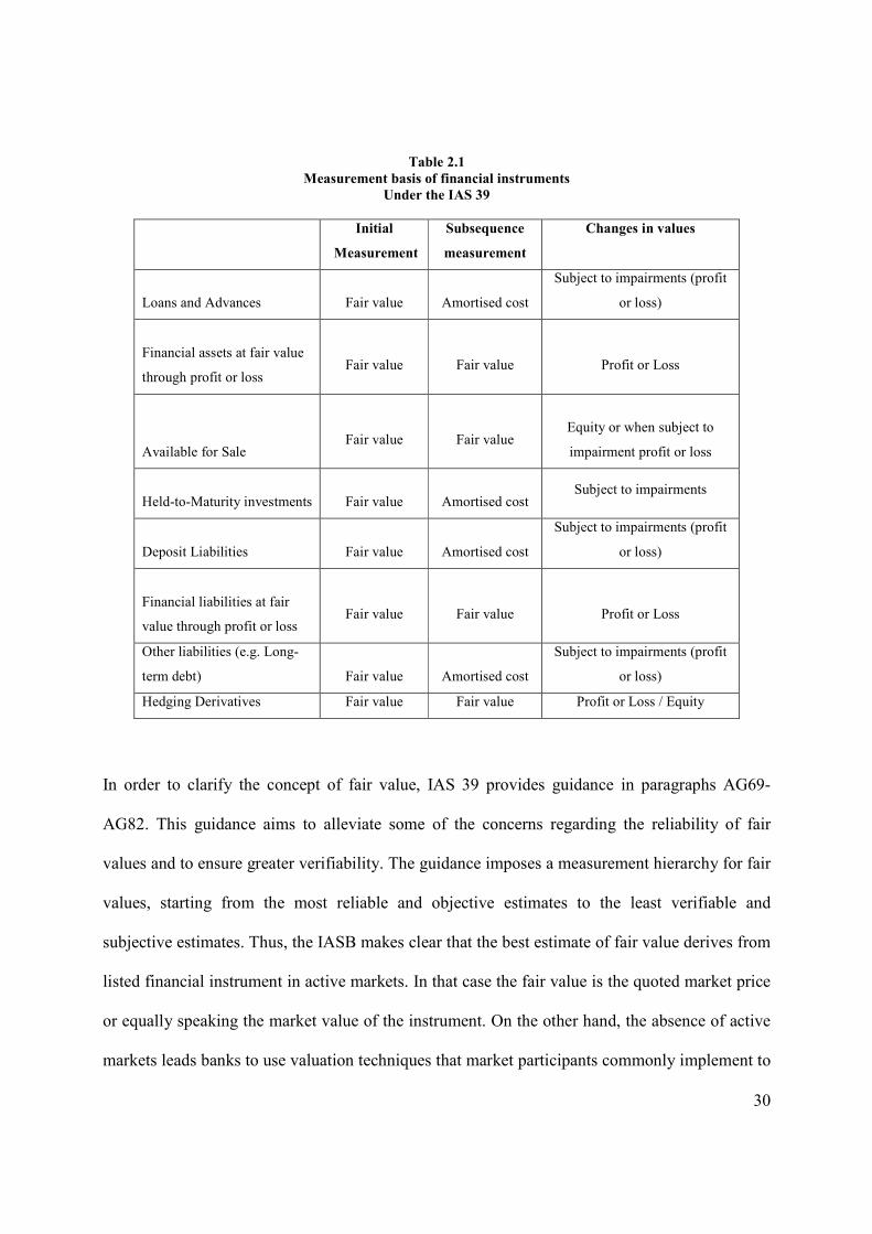
cost and the available-for-sales financial assets, are impaired. See table 2.1 for a summary on the

measurement bases of financial instruments under IAS 39.

Although IAS 39 requires specific categories of financial instruments to be recognised at

amortised cost, IAS 32 (and later IFRS 7) requires the disclosure of their fair values in the notes

to the financial statements for comparison. Thus, banks provide two values for the Loans and

Advances, Held to Maturity investments, Deposit Liabilities, Debt Securities, and Subordinated

Debt: the amortised cost which is recognised in the financial statements (required under IAS 39)

and the fair value which is disclosed in the notes to the financial statements (required under

IAS32/IFRS 7).

30

Table 2.1

Measurement basis of financial instruments

Under the IAS 39

Initial

Measurement

Subsequence

measurement

Changes in values

Loans and Advances

Fair value

Amortised cost

Subject to impairments (profit

or loss)

Financial assets at fair value

through profit or loss

Fair value

Fair value

Profit or Loss

Available for Sale

Fair value

Fair value

Equity or when subject to

impairment profit or loss

Held-to-Maturity investments

Fair value

Amortised cost Subject to impairments

Deposit Liabilities

Fair value

Amortised cost


or loss)

Financial liabilities at fair

value through profit or loss

Fair value

Fair value

Profit or Loss

Other liabilities (e.g. Long-

term debt)

Fair value

Amortised cost


or loss)

Hedging Derivatives Fair value Fair value Profit or Loss / Equity

In order to clarify the concept of fair value, IAS 39 provides guidance in paragraphs AG69-

AG82. This guidance aims to alleviate some of the concerns regarding the reliability of fair

values and to ensure greater verifiability. The guidance imposes a measurement hierarchy for fair

values, starting from the most reliable and objective estimates to the least verifiable and

subjective estimates. Thus, the IASB makes clear that the best estimate of fair value derives from

listed financial instrument in active markets. In that case the fair value is the quoted market price

or equally speaking the market value of the instrument. On the other hand, the absence of active

markets leads banks to use valuation techniques that market participants commonly implement to

31

estimate fair values, such as discounted cash flow models and option pricing models. To assure

greater reliability in estimating fair values using valuation techniques, the IASB requires firms to

base their estimates more on market inputs and less on entity-specific inputs (IAS 39, para.

AG75).

Thus, the fact that the fair value is not always a market value (mark-to-market), but also an

estimated amount (mark-to-model) makes the term “fair value” a broader concept than the term

“market value” even if sometimes these two values coincide (Khurana and Kim, 2003).

When banks calculate the fair value of a financial instrument should consider a number of

observable market factors that can affect its fair value. IAS 39 provides factors such as the time

value of money, credit risk, foreign currency exchange prices, commodity prices, equity prices,

volatility, prepayment risk and surrender risk, and servicing costs (IAS 39, para. AG82). For

example, a bank should account for interest rate changes when estimating the fair value of a loan

by discounting the loan’s expected cash flows with the prevailing interest rate.

Regarding deposit liabilities, which represent a major liability for banks, IAS 39 states that the

fair value of a financial liability with a demand feature, such as a demand deposit, can not be less

than the amount payable on demand (IAS 39, para 49). Hence, banks assume that the fair value

of demand deposits equals the carrying amount and no difference arises between the amortised

cost and the fair value. For all other deposits (i.e. term deposits) banks use discounted cash flow

models to estimate their fair values3.

3 Indicative extracts from the Annual Report 2006 of Lloyds TSB Group (p. 117) illustrate how banks estimate the fair values of loans and deposits in practice. A) For loans: “…For commercial and personal customers, fair value is

32

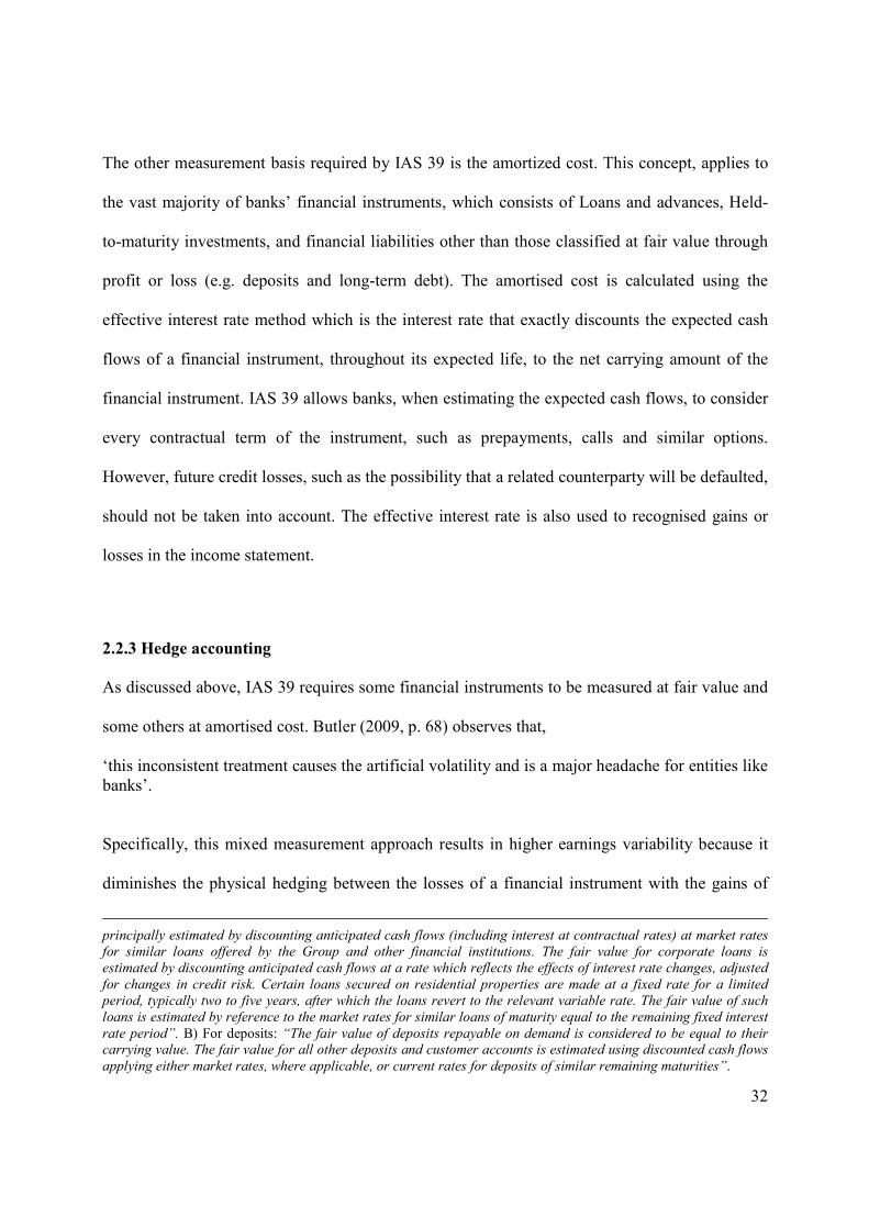
The other measurement basis required by IAS 39 is the amortized cost. This concept, applies to

the vast majority of banks’ financial instruments, which consists of Loans and advances, Held-

to-maturity investments, and financial liabilities other than those classified at fair value through

profit or loss (e.g. deposits and long-term debt). The amortised cost is calculated using the

effective interest rate method which is the interest rate that exactly discounts the expected cash

flows of a financial instrument, throughout its expected life, to the net carrying amount of the

financial instrument. IAS 39 allows banks, when estimating the expected cash flows, to consider

every contractual term of the instrument, such as prepayments, calls and similar options.

However, future credit losses, such as the possibility that a related counterparty will be defaulted,

should not be taken into account. The effective interest rate is also used to recognised gains or

losses in the income statement.

2.2.3 Hedge accounting

As discussed above, IAS 39 requires some financial instruments to be measured at fair value and

some others at amortised cost. Butler (2009, p. 68) observes that,

‘this inconsistent treatment causes the artificial volatility and is a major headache for entities like banks’.

Specifically, this mixed measurement approach results in higher earnings variability because it

diminishes the physical hedging between the losses of a financial instrument with the gains of

principally estimated by discounting anticipated cash flows (including interest at contractual rates) at market rates

for similar loans offered by the Group and other financial institutions. The fair value for corporate loans is

estimated by discounting anticipated cash flows at a rate which reflects the effects of interest rate changes, adjusted

for changes in credit risk. Certain loans secured on residential properties are made at a fixed rate for a limited

period, typically two to five years, after which the loans revert to the relevant variable rate. The fair value of such

loans is estimated by reference to the market rates for similar loans of maturity equal to the remaining fixed interest

rate period”. B) For deposits: “The fair value of deposits repayable on demand is considered to be equal to their

carrying value. The fair value for all other deposits and customer accounts is estimated using discounted cash flows

applying either market rates, where applicable, or current rates for deposits of similar remaining maturities”.

33

another financial instrument when they are all measured at fair values. Thus, the purpose of

hedge accounting is to provide an artificial match between gains and losses in order to reduce

risk.

According to IAS 39 (IAS 39, para 86), the hedging relationships can be of three types, namely:

a fair value hedge, a cash flow hedge, and a hedge of the net investment in a foreign operation.

As the term indicates, a fair value hedge aims to hedge banks’ exposure to changes in fair values

of recognised assets and liabilities and of unrecognised commitments. Similarly, the cash flow

hedge aims to hedge banks’ exposure against the variability of financial instruments’ cash flows.

Finally, a net investment hedge is a hedge of an entity’s interest in the net assets of that operation

against a foreign currency exposure.

The accounting treatment of the hedging activity depends on the type of the hedging discussed

above. If a hedging relationship is a fair value hedge then the gains and losses of both the

hedging instrument and the hedged item are recognised in the profit or loss for the year statement.

If a hedging relationship is a cash flow hedge or a hedge of net investment in a foreign operation

then the effective portion of the gains and losses on the hedging instrument is recognised in

equity, whilst the ineffective portion is recognised in the profit or loss statement.

IAS 39 imposes some restrictions as to which types of financial instruments can qualify for

hedge accounting. For example, it precludes the use of held-to-maturity investments as hedged

instruments, regarding the interest rate risk. Held-to-maturity investments are usually held to

maturity and thus changes in values are irrelevant. Furthermore, IAS 39 precludes the use of fair

34

value hedge accounting for demand deposits that are managed in a portfolio with other financial

assets and liabilities. This is the macro hedging activity of banks that it was also a core

disagreement between the EC and the IASB; this issue is discussed in the next section.

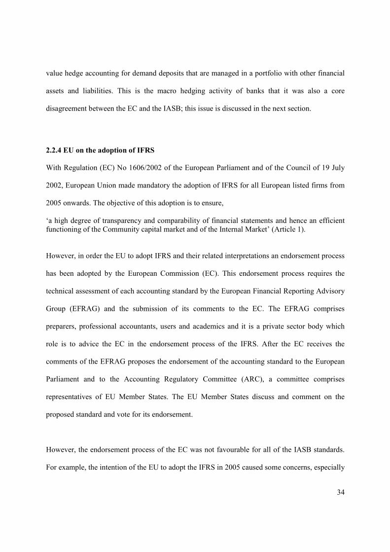
2.2.4 EU on the adoption of IFRS

With Regulation (EC) No 1606/2002 of the European Parliament and of the Council of 19 July

2002, European Union made mandatory the adoption of IFRS for all European listed firms from

2005 onwards. The objective of this adoption is to ensure,

‘a high degree of transparency and comparability of financial statements and hence an efficient functioning of the Community capital market and of the Internal Market’ (Article 1).

However, in order the EU to adopt IFRS and their related interpretations an endorsement process

has been adopted by the European Commission (EC). This endorsement process requires the

technical assessment of each accounting standard by the European Financial Reporting Advisory

Group (EFRAG) and the submission of its comments to the EC. The EFRAG comprises

preparers, professional accountants, users and academics and it is a private sector body which

role is to advice the EC in the endorsement process of the IFRS. After the EC receives the

comments of the EFRAG proposes the endorsement of the accounting standard to the European

Parliament and to the Accounting Regulatory Committee (ARC), a committee comprises

representatives of EU Member States. The EU Member States discuss and comment on the

proposed standard and vote for its endorsement.

However, the endorsement process of the EC was not favourable for all of the IASB standards.

For example, the intention of the EU to adopt the IFRS in 2005 caused some concerns, especially

35

in relation to standards dealing with financial instruments (IAS 32 and 39). The two most

important concerns were the fair value option and the macro hedging (BIS, 2004a; EBF, 2003).

These concerns led the EU to endorse the IAS 32 and 39 with two major ‘carve-outs’ until the

IASB reconsiders the issues. Thus, the paragraphs, relating to the fair value option and the macro

hedging, have not been included in the version of IAS 39 that was adopted by the EU. All other

standards were endorsed by the EU as published by the IASB.

The fair value option permitted firms to measure upon initial recognition all financial assets and

liabilities at fair value without any restriction (IAS 39). This statement caused the reaction of the

European Central Bank (hereafter, ECB) and of prudential supervisors represented in the Basel

Committee who argued that the fair value option could be used inappropriately by firms,

especially for their liabilities (BIS, 2004a). These concerns caused the IASB on 16 June 2005 to

issue amendments to the fair value option in IAS 39. The amendments restricted the use of the

fair value option to specific circumstances. For example, when it eliminates or reduces

accounting mismatches, when a group of financial assets and liabilities is managed and evaluated

at fair value due to risk management purposes, and when an instrument contains an embedded

derivative.

The macro hedging has been raised by European banks through their representative body, the

European Banking Federation (EBF, 2003). European banks argued that IAS 39 restricts the

application of hedge accounting for demand deposits by not permitting the use of fair value

hedge accounting for such instruments. This is because the IAS 39 requires that the fair value of

a demand liability is not less than the amount payable on demand (IAS 39, para 49). This rule

36

became an obstacle for banks to apply the fair value hedging to a portfolio of financial assets and

liabilities that includes demand deposits. Banks were concerned that this prohibition will force

them to change their asset-liability management and to incur addition costs to their accounting

systems. Banks classify their financial instruments in portfolios based on their expected

maturities to manage risk. The argument of banks is that the expected maturities of demand

deposits in aggregate (i.e. core deposits) usually differ significantly from their contractual

maturities (on demand). Based on historical statistical observations, the expected maturities of

demand deposits are longer than on demand. Thus, using discounted cash flow models, the fair

value of demand deposits in aggregate is usually a smaller amount than the amount payable on

demand. However, as stated above, the IAS 39 in paragraph 49 does not allow the fair value of a

liability to be less than the amount payable on demand. This restricted banks to follow their

asset-liability management for their macro hedging activity.

The amendment of the fair value option by the IASB on 16 June 2005 has been endorsed by the

EC on 15 November 2005, and finally the IASB and the EC came into an agreement. On the

other hand, no agreement has yet been achieved regarding the macro hedging, and thus the EC

has adopted a version of the IAS 39 that excludes the provisions for the macro hedging

restrictions.

The other important involvement of the EU in accounting standard setting was in 2008 when the

credit crunch forced many banks to write-down huge amount of losses in financial assets, such as

subprime loans. Arguably, the measurement of financial instruments at fair value became a

difficult procedure in inactive markets; hence fair value is not the ideal measurement method for

37

recognising assets in a forced liquidation or a distressed sale. Furthermore, accounting rules have

been criticised for causing market volatility. This led many European politicians, including the

French President Nicola Sarkozy, to ask the IASB to suspend mark-to-market accounting and

change the rules on fair values. Finally, in 13 October 2008, the IASB succumbed to pressures

and permitted the reclassification of financial assets (other than derivatives) out of the fair value

through profit or loss category.

2.2.5 A new standard on financial instruments (IFRS 9)

IAS 39 has been criticized for its complexity by preparers of financial statements, auditors, and

users (IASB, 2008). Since its publication in 1999 the IASB received numerous comments and

suggestions to improve accounting for financial instruments and to simplify the rules. The

pressure for a change was intensified during the financial crisis of 2008 when accounting

standards, and specifically IAS 39, were blamed for amplifying volatility due to the huge write-

downs of losses relating to the fair values of banks’ financial instruments.

This criticism led the IASB to re-examine accounting rules and gradually to replace completely

IAS 39. Towards this aim, the IASB issued in November 2009 a new standard, the IFRS 9

“Financial instruments” which consists of the first phase of a project to replace IAS 39. This

version of IFRS 9 discusses only the classification and measurement of financial assets. It was

re-issued in October 2010; this version includes the requirements on accounting for financial

liabilities. The effective date of mandatory adoption is 1 January 2013, with early adoption

permitted for the year-end 2009.

38

The aim of the IASB with IFRS 9 is to reduce complexity, improve comparability, and aid

investors to understand better accounting for financial instruments. The differences between the

old standard, IAS 39, and the new standard, IFRS 9, are remarkable. IFRS 9 eliminates two

broad categories of financial instruments, those of available-for-sale assets and held-to-maturity

investments. Financial assets are now classified according to their measurement basis, namely: as

at fair values or at amortized cost. IFRS 9 adopts a new approach to classify financial assets

based on two criteria: the objective of the entity’s business model and the contractual cash flows

of the financial asset. Each entity first considers its business model regarding its purpose to hold

financial assets to collect contractual cash flows, as opposed to holding financial assets to realise

short-term returns. The business model test is not necessarily performed separately for each

asset, but can be applied to aggregated assets. On the other hand, the contractual cash flow

characteristic test should be applied on an asset and only for assets that are measured at

amortized cost because of the business model criterion. According to the contractual cash flow

characteristic, the contractual terms of a financial asset should give rise at specific dates to cash

flows that are solely payments of principal and interest on the principal outstanding.

The debt instruments are measured at amortized cost if both the business model test and the cash

flow characteristic test are met. All other debt instruments should be recognised at fair value.

Equity instruments that are held for speculation should be measured at fair value with changes

recognised in the income statement. A new category of financial assets is the equity investments

with no trading objective. These financial instruments should be also measured at fair value but

their changes are recorded to other comprehensive income instead of the income statement.

39

However, IFRS 9 makes clear that any dividends arising from these instruments should be

recognised in the income statement.

Another important change between the provisions of IAS 39 and IFRS 9 is the different

treatment of equity instruments and derivatives that do not have quoted market prices and their

fair value cannot be estimated reliably. Whilst IAS 39 required their recognition at cost, IFRS 9

requires their measurement at fair value. Finally, all derivatives should be measured at fair value

through profit or loss. However, IFRS 9 gives the option to firms to continue treat hedging

derivatives as required under IAS 39 (see, Section 2.2.3).

The fair value option, which was also present in IAS 39, is permitted by IFRS 9. This rule

applies to all financial assets and allows a firm to designate a financial asset upon initial

recognition at fair value through profit or loss given that this treatment eliminates accounting

mismatches. Finally, reclassifications from the amortized cost category to the fair value category

and vice versa are not prohibited, but they need to be based on changes of the entity’s business

model which are usually rare.

2.2.6 US GAAP on financial instruments

Up to now the accounting for financial instruments is examined within the context of IFRS.

However, a brief mention should be made to the US GAAP for two reasons. First, most of the

value relevance studies on financial instruments are within the context of US accounting

standards, and second both the IASB and the FASB collaborate to produce common rules

40

regarding financial instruments or to eliminate the differences (see, Memorandum of

Understanding between the FASB and the IASB, 2006).

US GAAP addresses accounting for financial instruments in a number of standards. The first

standard that included disclosure requirements for financial instruments was SFAS No. 105

“Disclosure of Information about Financial Instruments with Off-Balance-Sheet Risk and

Financial Instruments with Concentrations of Credit Risk” (FASB, 1990). Specifically, it

required the disclosure of notional principal amounts, the term of the instruments, and possible

losses arise from contracts with off-balance sheet risk (this standard was superseded by SFAS

No. 133 (FASB, 1998)).

An important US standard on this issue was SFAS No. 107 “Disclosures about fair value of

financial instruments” (FASB, 1991). It was the first US standard that required the disclosure of

the fair values of all financial assets and liabilities, either recognised or not in the financial

statements. Although some US firms were disclosing voluntarily the fair values of some financial

instruments, SFAS No. 107 made this disclosure mandatory for both on and off-balance sheet

instruments.

Similar to IAS 39 classification, SFAS No. 115 “Accounting for certain investments in debt and

equity securities” (FASB, 1993) addressed the accounting and reporting for investments in

equity securities (that have readily determinable fair values) and for investments in debt

securities. This standard classifies debt and equity securities in three categories: i) Held-to-

maturity securities (debt instruments where the entity have the ability and intend to hold to

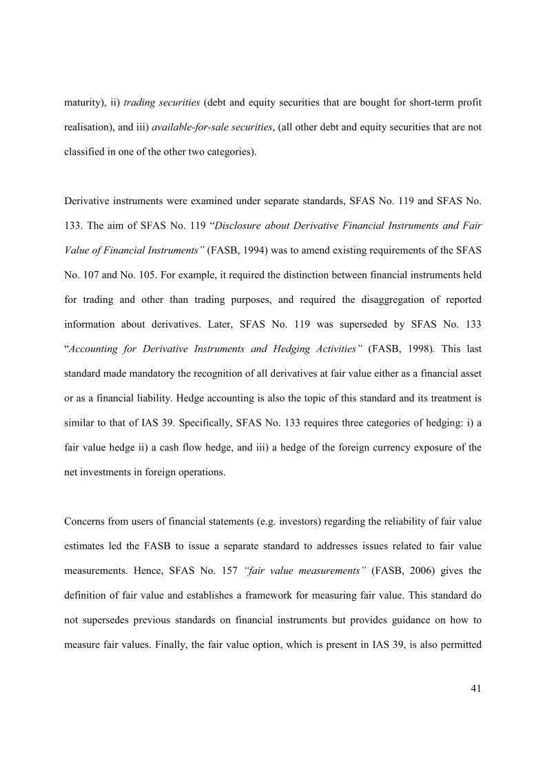
41

maturity), ii) trading securities (debt and equity securities that are bought for short-term profit

realisation), and iii) available-for-sale securities, (all other debt and equity securities that are not

classified in one of the other two categories).

Derivative instruments were examined under separate standards, SFAS No. 119 and SFAS No.

133. The aim of SFAS No. 119 “Disclosure about Derivative Financial Instruments and Fair

Value of Financial Instruments” (FASB, 1994) was to amend existing requirements of the SFAS

No. 107 and No. 105. For example, it required the distinction between financial instruments held

for trading and other than trading purposes, and required the disaggregation of reported

information about derivatives. Later, SFAS No. 119 was superseded by SFAS No. 133

“Accounting for Derivative Instruments and Hedging Activities” (FASB, 1998). This last

standard made mandatory the recognition of all derivatives at fair value either as a financial asset

or as a financial liability. Hedge accounting is also the topic of this standard and its treatment is

similar to that of IAS 39. Specifically, SFAS No. 133 requires three categories of hedging: i) a

fair value hedge ii) a cash flow hedge, and iii) a hedge of the foreign currency exposure of the

net investments in foreign operations.

Concerns from users of financial statements (e.g. investors) regarding the reliability of fair value

estimates led the FASB to issue a separate standard to addresses issues related to fair value

measurements. Hence, SFAS No. 157 “fair value measurements” (FASB, 2006) gives the

definition of fair value and establishes a framework for measuring fair value. This standard do

not supersedes previous standards on financial instruments but provides guidance on how to

measure fair values. Finally, the fair value option, which is present in IAS 39, is also permitted

42

by the FASB under certain conditions (see, SFAS No. 159 “The Fair Value Option for Financial

Assets and Financial Liabilities” (FASB, 2007)).

2.3 Capital regulations for commercial banks

2.3.1 The need for regulation

Commercial banks perform a vital role in an economy. They act as financial intermediaries

between borrowers and savers as they transfer money from people and organizations that have

surplus of funds to those that have deficit of funds (Casu et al., 2006). In other words, they

collect money from the public via deposits and allocate them to productive activities in the

economy by giving loans. This operation of banks contributes significantly to the economic

growth of a country. This sensitive role of banks makes necessary their regulation by imposing

restrictions on minimum capital requirements. In theory, regulation promotes public confidence

and alleviates concerns that a bank will go bust.

2.3.2 The 1988 Capital Accord (Basel I)

Traditionally, the regulation of commercial banks was performed by central banks. Specifically,

for the euro zone, this role is undertaken by the ECB with the cooperation of the independent

central banks based around the EU countries. Central banks also have their own “bank”, the

Bank for International Settlements (BIS), which is an international organization with members

the majority of the central banks of the developed and developing countries. BIS states that the

objective of the organization is to ‘foster international monetary and financial cooperation, and to

serve as a bank for central banks’ (Available from: www.bis.org/ [Accessed 1 September 2009]).

43

In order to achieve its objective, BIS operates a number of committees that discuss on a regular

basis monetary and financial matters. Such a committee is the Basel Committee on Banking

Supervision (hereafter Basel Committee) which aims to improve banking supervision by

developing capital adequacy rules for commercial banks. The Basel Committee published in

1988 the “Capital Accord” which was the first attempt to provide details on how banks shall

measure capital adequacy and minimum capital requirements. Under the Capital Accord the

capital adequacy of a bank is determined using the Capital Adequacy Ratio (CAR) as presented

below:

CAR = Tier 1 + Tier 2

On and off-balance sheet assets (weighted by credit risk)

The numerator of this ratio consists of a bank’s capital. According to the Basel Committee, this

capital is separated between two elements, the core capital, widely known as the Tier 1 and the

supplemental capital, widely known as the Tier 2. Tier 1 capital consists of the i) banks’ equity

capital, and ii) the published reserves from post-tax retained earnings. Tier 2 capital comprises of

i) Undisclosed reserves, ii) Asset revaluation reserves, iii) General provisions/general loan loss

reserves, iv) Hybrid debt capital instruments, and v) Subordinated term debt4.

The denominator of the ratio is the on and off-balance sheet assets of a bank, weighted by credit

risk. The rationale behind this ratio is that banks should keep a minimum amount of capital

relative to their credit risk that can cover future potential losses. Therefore, assets in the

denominator are classified based on their credit risk by specifying risk weights for each bank’s

4 Certain deductions should be made from Tier 1 and Tier 2 capital. Specifically, goodwill needs to be deducted from the Tier 1 capital and investments and subsidiaries from the total capital base (Tier 1 + Tier2).

44

asset. Specifically, it assigns no risk (0%) to cash and claims on central governments and central

banks, low risk (20%) to claims on banks incorporated in the OECD and to short-term claims

with maturities a year or less, moderate risk (50%) to mortgages, and high risk (100%) to claims

to the private sector, such as commercial loans. In addition, the Capital Accord assigns to all off-

balance sheet items equivalent weights based on their credit risk.

The ratio above indicates that banks with more low credit risk assets have higher capital

adequacy ratios, and thus lower possibility to be in trouble due to customer defaults. According

to the Basel Committee, each commercial bank needs to maintain a CAR above 8%. In addition

the Tier 1 capital to weighted assets (i.e. Tier 1/weighted assets) should be above 4%. It also

requires that the Tier 1 capital should be at least 50% of the total bank’s capital base (Tier 1 and

Tier 2).

2.3.3 Basel Amendments (1996) to incorporate market risk

The Capital Accord focused only on credit risk, ignoring other important types of risk, such as

market risk5. This led to criticism of the Basel Accord’s approach of measuring capital adequacy

and urged Basel Committee to re-examine rules on capital in order to incorporate market risk.

The assets of banks that are most vulnerable to market risk are those in their trading book which

consist primarily of short-term positions usually held for speculation.

In order to improve the 1988 Basel Accord, the Basel Committee issued in 1996 specific

amendments to incorporate the market risk in measuring capital requirements. Specifically, it

5 Market risk arises from the fluctuation in values of banks’ assets caused by changes in market prices of equities, interest rates, exchange rates, the commodities’ prices and any other changes in market values.

45

introduced a third type of capital in the numerator of CAR, the Tier 3 capital. This capital

consists of short-term subordinated debt and can be used solely to support the market risk. This

means that the Tier 1 and Tier 2 capital will continue to cover the credit risk including the credit

counterparty risk with respect to derivatives in both the trading and the banking books. Tier 3

capital is limited to up to 250% of the Tier 1 capital.

In order for both the credit risk and the market risk to be incorporated consistently into the

calculations of the CAR, the measure of market risk should be multiplied by 12.5 (which is the

reciprocal of the minimum CAR of 8%) and then added to the risk-weighted assets relating to the

credit risk. Thus the CAR under these calculations represents the capital that is available to cover

both types of risk, the credit and the market risk.

2.3.4 Basel II – The Three Pillar Approach

The amendments introduced in 1996 to overcome the criticisms of the Capital Accord proved

insufficient. Further discussions between the Basel Committee on Banking Supervision and other

constituents, such as bankers, resulted in the publication of a new document in 2004 titled,

“International Convergence of Capital Measurement and Capital Standards: a Revised

Framework” (BIS, 2004b). This document proposes a new framework to measure banks’ credit

risk and introduces three pillars that aim to provide a holistic approach in measuring banks’

capital adequacy.

The first pillar aims to quantify banks’ risk and to set minimum capital requirements to support

the risk undertaken by financial institutions. It allows banks to adopt new measures of credit risk

46

by examining the creditworthiness of their counterparties in detail and not by applying the “one

size fits all” approach which was used by Capital Accord. Banks can use both internal risk

ratings and external credit risk assessments in order to evaluate the credit risk. Furthermore,

Basel II introduces a new type of risk, the operational risk defined as ‘the risk of loss resulting

from inadequate or failed internal processes, people and systems or from external events’. The

rules regarding the measurement of market risk have not changed since the amendments in 1996.

Thus, under Basel II the CAR is expanded to include three types of risk in the denominator,

namely: the unchanged measures of market risk (the amendments of the Capital Accord in 1996);

new measures of credit risk (as discussed above); and the operational risk. Tier 1 and Tier 2

capital in the numerator are kept unchanged as well as the minimum capital adequacy ratio of 8%

for the total CAR (Tier 1 and 2) and the 4% requirement for the ratio of Tier 1 capital to

weighted assets.

The second pillar is referred to as the supervisory review process. Under this pillar supervisors

should closely monitor banks’ activities and risks and provide guidance on the minimum amount

of capital that should be kept separately by each bank in order to support the undertaken risk.

Furthermore, supervisors should encourage banks to develop their own risk management systems

and to improve their risk measurement techniques regarding their financial instruments.

Moreover, supervisors have the right to require banks to hold more capital than the minimum

requirements (i.e. 8%) if they believe that some banks undertake excessive risk.

Finally, the third pillar is a supportive function of the first two pillars. It requires banks to

disclose a substantial amount of information to the financial community (e.g. analyst and

47

investors in general) relating to the capital requirement of banks. In particular, banks need to

disclose information such as the risk exposure, the methods they use to calculate capital

adequacy, and details of their risk management techniques.

Following the financial crisis of 2008, Basel Committee moved again to improve banks capital

regulations by introducing stricter rules. This movement is called the ‘Basel III’ and intends to

strengthen banks’ capital and improve liquidity rules. For example, it gradually increases the

minimum capital for the Tier 1 ratio from 4% to 6% until the 1st of January 2015. The total

capital requirement is retained at 8%.

2.3.5 EU on Capital Adequacy Requirements

The EU promoted the adoption of a single set of rules on capital adequacy requirements that aim

to strengthen the credibility of financial institutions while at the same time it hoped that they

would boost the functioning of an integrated European economy. The Codification of Banking

Directive (2000/12/EC), which was a consolidation of two Directives of the EC (the Directive of

solvency ratio (89/647/EEC) and the Directive of own funds (89/299/EEC)), together with the

Directive of the capital adequacy of investment firms and credit institutions (93/6/EEC)

constitute the EU legislation framework that incorporates the requirements of the Basel Accord.

These laws apply to all credit institutions and investment firms in the EU.

The issue of new capital rules (the Basel II) by the Basel Committee in 2004 led the EU to

commence all the necessary procedures in order to incorporate the new capital adequacy

requirements into its own legislation. The outcome of the discussions resulted in the Capital

48

Requirements Directive (CRD) that consists of the Directive 2006/49/EC on the capital adequacy

of investment firms and credit institutions and the Directive 2006/48/EC which relates to the

taking up and pursuit of the business of credit institutions. These two Directives form an

equivalent agreement to the provisions of the Basel II framework. The new EU law came into

force on the 1st of January 2007 and was fully adopted by the 1st of January 2008.

2.4 Conclusion

This Chapter explored the regulations within which European commercial banks operate by

analysing the accounting and capital adequacy rules that apply to these institutions. Accounting

for financial instruments was the focus of the analysis as they dominate banks’ financial

statements. All European listed firms were required to follow the IFRS from 2005, and thus the

discussion is performed within the IFRS context, covering accounting standards on financial

instruments, such as the IAS 32, IAS 39, and the IFRS 7. However, the US GAAP was also

discussed for two reasons: i) there is a tendency during the last few years between the IASB and

the FASB to develop a common set of accounting standards, and specifically, to achieve

converge on financial instrument rules (see, IASB and FASB’s “Norwalk Agreement”)6, ii) for

comparison, as most value relevance studies on financial instruments use US GAAP. Finally, the

Chapter discussed the capital adequacy rules, such as the Capital Accord requirements and the

Basel II provisions to which Banks are subjected. This was necessary given the fact that a

number of variables in this thesis are based on banks’ capital adequacy ratios.

6 Available from: http://www.fasb.org/news/memorandum.pdf, [Accessed 17 March 2009].

49

Chapter 3: Theoretical Framework

3.1 Introduction

This chapter discusses the theoretical framework of the thesis which is the equity valuation

theory. Both value relevance research and cost of equity research, which this thesis deals with,

are based on this framework. The chapter also explains the relationship between CE and

accounting standards which provides the argument regarding why one should expect that the

adoption of IFRS will reduce the CE. Finally, a critical view of the value relevance research is

discussed.

Barth (2006b) defines value relevance as ‘the relation between share prices, or returns, and

accounting information’. Equity valuation theory provides models that link accounting numbers

to market values, and not surprisingly these models have been used extensively in the value

relevance research (Barth et al., 1996; Eccher et al., 1996; Nelson, 1996; Wang et al., 2005).

Equity valuation theory also provides the theoretical framework for the second part of the thesis

which examines the effects that the mandatory adoption of IFRS has on banks’ cost of equity

(See, the second research objective in Chapter 1). CE, however, is not observable and needs to be

estimated. Equity valuation models provide us with the equity value of a firm given its CE. Most

of the inputs of equity valuation models can be found from published figures, such as share

prices and firms’ expected earnings, and therefore, it is possible to infer the CE under certain

assumptions. Although, this is not the only approach for obtaining the CE (e.g. early studies used

the CAPM that uses historical observations to derive the require rate of return (i.e. the CE)) it is

now the most popular in the accounting literature (Gebhardt et al., 2001).

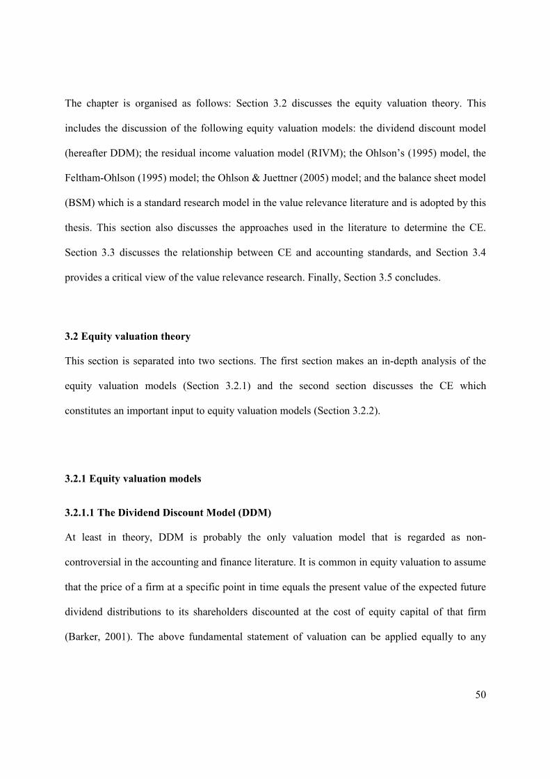
50

The chapter is organised as follows: Section 3.2 discusses the equity valuation theory. This

includes the discussion of the following equity valuation models: the dividend discount model

(hereafter DDM); the residual income valuation model (RIVM); the Ohlson’s (1995) model, the

Feltham-Ohlson (1995) model; the Ohlson & Juettner (2005) model; and the balance sheet model

(BSM) which is a standard research model in the value relevance literature and is adopted by this

thesis. This section also discusses the approaches used in the literature to determine the CE.

Section 3.3 discusses the relationship between CE and accounting standards, and Section 3.4

provides a critical view of the value relevance research. Finally, Section 3.5 concludes.

3.2 Equity valuation theory

This section is separated into two sections. The first section makes an in-depth analysis of the

equity valuation models (Section 3.2.1) and the second section discusses the CE which

constitutes an important input to equity valuation models (Section 3.2.2).

3.2.1 Equity valuation models

3.2.1.1 The Dividend Discount Model (DDM)

At least in theory, DDM is probably the only valuation model that is regarded as non-

controversial in the accounting and finance literature. It is common in equity valuation to assume

that the price of a firm at a specific point in time equals the present value of the expected future

dividend distributions to its shareholders discounted at the cost of equity capital of that firm

(Barker, 2001). The above fundamental statement of valuation can be applied equally to any

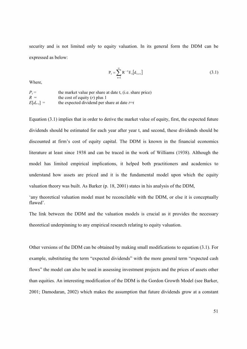
51

security and is not limited only to equity valuation. In its general form the DDM can be

expressed as below:

[ ]∑∞

=+

−=1τ

τttτ

t dERP (3.1)

Where, Pt = the market value per share at date t, (i.e. share price) R = the cost of equity (r) plus 1 E[dt+τ] = the expected dividend per share at date t+τ

Equation (3.1) implies that in order to derive the market value of equity, first, the expected future

dividends should be estimated for each year after year t, and second, these dividends should be

discounted at firm’s cost of equity capital. The DDM is known in the financial economics

literature at least since 1938 and can be traced in the work of Williams (1938). Although the

model has limited empirical implications, it helped both practitioners and academics to

understand how assets are priced and it is the fundamental model upon which the equity

valuation theory was built. As Barker (p. 18, 2001) states in his analysis of the DDM,

‘any theoretical valuation model must be reconcilable with the DDM, or else it is conceptually flawed’. The link between the DDM and the valuation models is crucial as it provides the necessary

theoretical underpinning to any empirical research relating to equity valuation.

Other versions of the DDM can be obtained by making small modifications to equation (3.1). For

example, substituting the term “expected dividends” with the more general term “expected cash

flows” the model can also be used in assessing investment projects and the prices of assets other

than equities. An interesting modification of the DDM is the Gordon Growth Model (see Barker,

2001; Damodaran, 2002) which makes the assumption that future dividends grow at a constant

52

rate in perpetuity. The Gordon growth model can be easily derived by simple mathematical

transformations of Equation (3.1):

gr

dP 1t

t −= + (3.2)

The constant term g in equation (3.2) denotes growth in dividends. Assuming that dividends

grow at a constant percentage, the model requires only the estimation of three parameters,

namely: next period’s dividends dt+1, the cost of equity capital r, and the growth in dividends g.

Equation (3.2) demands r to be greater than g otherwise the value of the asset would be negative.

3.2.1.2 The Residual Income Valuation Model (RIVM)

As analysed above the market value of equity in the context of DDM is based only on expected

dividends (i.e. cash flows to equity), given the cost of equity capital. However, other valuation

models, such as the RIVM, use solely accounting information inputs. As Rees (1995) and Lee

(1999) observe RIVM is not new in the accounting literature, but can be traced in the works of

Preinreich (1938), Edwards & Bell (1961), Edey (1962) and Peasnell (1982). Under this model,

the market value of equity is the outcome of two accounting constructs i) the book value of

equity, and ii) the present value of abnormal earnings. Mathematically this relationship can be

expressed as follows:

[ ]∑∞

=+

−+=1τ

ατtt

τtt xΕRbvP (3.3)

Where: bvt = book value of equity at time t

[ ]ατtt xE + = expected abnormal earnings at date t+τ

53

Ohlson (1995, p. 667) defines abnormal earnings as the excessive amount of earnings over

“normal” earnings. “Normal” earnings are the anticipated return on the beginning of the period

book value of equity (the return that investors expect to earn). This anticipated return can be

expressed as the product of the beginning of the period book value of equity at date t-1 and the

cost of equity capital (r). Thus using symbols abnormal earnings are defined as follows:

1ttαt bvrxx −×−= (3.4)

Where tx is actual earnings for the period (t). RIVM (Equation 3.3.) assumes that the book value

of equity (bv) underestimates the market value of equity, due to conservative accounting, and

thus an additional construct is necessary to capture the difference between the book value and the

market value of equity. This additional construct is the present value of all future abnormal

earnings which alternatively can be viewed as a firm’s goodwill. It is reasonable to assume that

under an accounting system where all assets and liabilities are measured at market value, the

book value of equity (bv) equals the market value (P) and thus the present value of abnormal

earnings in equation (3.3) is zero ( [ ]∑∞

=+

−

1τ

α

τtt

τ xΕR = 0). In all other circumstances P≠ bv and thus

the term [ ]∑∞

=+

−

1τ

α

τtt

τ xΕR ≠ 0. Usually in practice bv < P due to conservative accounting and as a

consequence the present value of abnormal earnings is a positive number.

Substituting equation (3.4) into equation (3.3) and making some simple transformations we can

have a different interpretation of RIVM using the relationship (3.5).

( )[ ]∑∞

=−++ −+=

1

1τtτttτ-

tt bvrROEERbvP

τ

(3.5)

54

Equation (3.5) implies that Pt = bvt if and only if future ROE equals firm’s cost of equity capital

(r). ROEt denotes the return on equity at date t and is defined as the ratio of earnings at date t

divided by the book value of equity at the beginning of the period t-1. In a highly competitive

business environment ROE equals cost of equity capital (r) as firms do not have significant

competitive advantages to support excessive earnings. In a different situation, firms possessing

some forms of competitive advantages have a ROE that is greater than r and as a consequence

their P is greater than bv. However, even in a competitive business environment ROE may differ

from r due to conservative accounting (Frankel & Lee, 1998).

Returning back to the statement of Barker (2001) that every valuation model must be reconciled

to the DDM in order to be theoretical consistent it will be an omission not to present the link

between the DDM and the RIVM. Clean Surplus Relation (CSR) provides this link. The term

Clean Surplus Relation means that all gains and losses pass through the income statement in a

way that the difference between the book value of equity at the end of the period t and at the

beginning of the period t-1 equals earnings at date t minus dividends at date t.

tt1tt dxbvbv −=− − or

t1ttt dbvbvx +−= − (3.6)

Substituting Equation (3.6) into (3.4) and making some arrangements we can express dividends

(dt) as follows:

tαt1tt bvxbvRd −+×= − , where R=r+1 (3.7)

Substituting Equation (3.7) into Equation (3.1) (the DDM formulae), we obtain the RIVM, see

Equation (3.3). Thus, the link between the DDM and the RIVM is justified by assuming that the

accounting system follows the Clean Surplus Relation. The empirical failure of the RIVM to

55

capture market value of equity can be interpreted as a rejection of the DDM, which is the

fundamental valuation model. However, Lo & Lys (2000) argue that this is a naive conclusion

given that RIVM requires prediction of future expected earnings which are usually vulnerable to

measurement errors. Thus, failure of the RIVM to estimate share prices can be attributed to the

noise arising from the input data and not from the misspecification of the model. Lo & Lys (2000)

conclude that the RIVM is ‘…neither implementable nor testable’ and that the contribution of

Ohlson (1995) in the valuation theory is the transformation of the RIVM to an empirically

testable valuation model using Information Dynamics (ID).

3.2.1.3 The Ohlson (1995) model

Ohlson (1995) developed a parsimonious valuation model which links market values to

contemporaneous accounting data. The formulation of the model is based on three

straightforward assumptions. The first one is that the model builds on the neoclassical approach

to equity valuation that of the DDM. The second assumption relates to a Clean Surplus Relation

accounting system where the book value of equity at the end of the year equals the book value of

equity at the beginning of the year plus year’s earnings minus dividends. One can easily observe

that the first two assumptions are the ones that are also used to derive the RIVM. However, the

contribution of Ohlson to equity valuation theory relates to his third assumption, the Information

Dynamics (ID), which impose that the abnormal earnings follow an autoregressive process of

AR(1).

RIVM demands the prediction of abnormal earnings. In order to estimate these predictions,

Ohlson (1995) assumes a linear relationship for abnormal earnings as follows:

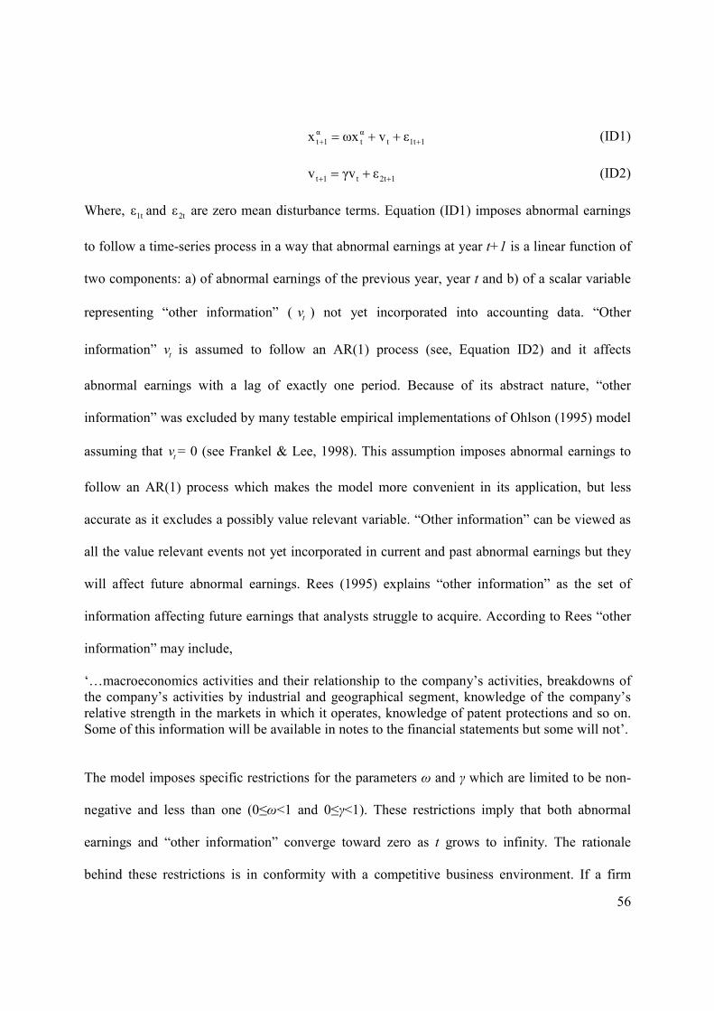
56

11tt

α

t

α

1t εvωxx ++ ++= (ID1)

12tt1t εγvv ++ += (ID2)

Where, 1tε and 2tε are zero mean disturbance terms. Equation (ID1) imposes abnormal earnings

to follow a time-series process in a way that abnormal earnings at year t+1 is a linear function of

two components: a) of abnormal earnings of the previous year, year t and b) of a scalar variable

representing “other information” ( tv ) not yet incorporated into accounting data. “Other

information” tv is assumed to follow an AR(1) process (see, Equation ID2) and it affects

abnormal earnings with a lag of exactly one period. Because of its abstract nature, “other

information” was excluded by many testable empirical implementations of Ohlson (1995) model

assuming that tv = 0 (see Frankel & Lee, 1998). This assumption imposes abnormal earnings to

follow an AR(1) process which makes the model more convenient in its application, but less

accurate as it excludes a possibly value relevant variable. “Other information” can be viewed as

all the value relevant events not yet incorporated in current and past abnormal earnings but they

will affect future abnormal earnings. Rees (1995) explains “other information” as the set of

information affecting future earnings that analysts struggle to acquire. According to Rees “other

information” may include,

‘…macroeconomics activities and their relationship to the company’s activities, breakdowns of the company’s activities by industrial and geographical segment, knowledge of the company’s relative strength in the markets in which it operates, knowledge of patent protections and so on. Some of this information will be available in notes to the financial statements but some will not’.

The model imposes specific restrictions for the parameters ω and γ which are limited to be non-

negative and less than one (0≤ω<1 and 0≤γ<1). These restrictions imply that both abnormal

earnings and “other information” converge toward zero as t grows to infinity. The rationale

behind these restrictions is in conformity with a competitive business environment. If a firm

57

possesses a competitive advantage generating positive abnormal earnings this will attract other

firms to enter into the same market in order to benefit from the excessive profits that the market

generates. In the long-run competition will diminish every competitive advantage that firms have

and thus abnormal earnings will converge toward zero.

Parameters ω and γ can also be interpreted as being the persistence parameters of a

tx and tv . The

closer these parameters are to unity the longer the competitive advantages will last for firms and

the slower the abnormal earnings and “other information” will converge to zero. It is worthwhile

to state that in the long-run both a

tx and tv asymptotically converge to zero.

Based on the three assumptions above, namely: the DDM, the Clean Surplus Relation and the

Information Dynamics, Ohlson (1995) derives a linear equity valuation model that expresses the

equity value of a firm as a linear function of i) current book value of equity, ii) current abnormal

earnings, and iii) “other information”.

t2

α

t1tt vαxαbvP ++= (3.8)

Where, ( ) 0ωRω/α1 ≥−=

( )( ) 0γRωRR/α2 >−−=

The advantage of the Ohlson (1995) model over the RIVM is that it uses contemporaneous

numbers to derive firm’s market value of equity, whilst RIVM relies on the prediction of future

abnormal earnings. However the modelling of Ohlson’s (1995) “other information” is still a

controversial issue in the literature.

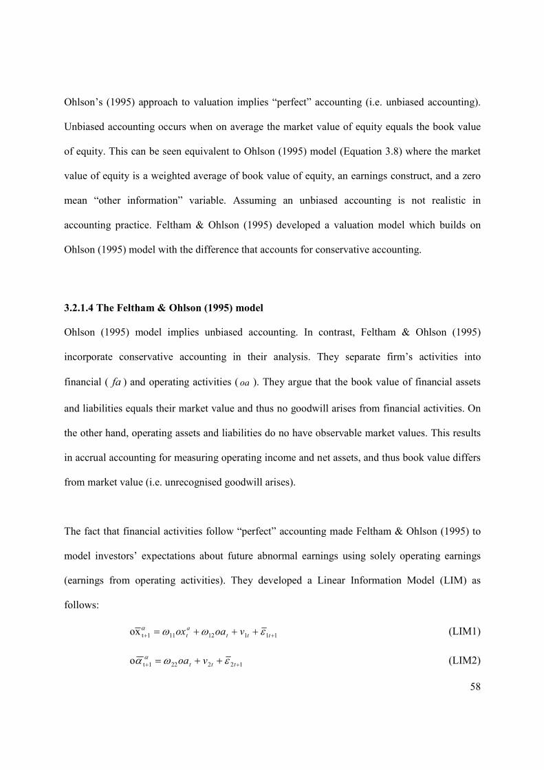
58

Ohlson’s (1995) approach to valuation implies “perfect” accounting (i.e. unbiased accounting).

Unbiased accounting occurs when on average the market value of equity equals the book value

of equity. This can be seen equivalent to Ohlson (1995) model (Equation 3.8) where the market

value of equity is a weighted average of book value of equity, an earnings construct, and a zero

mean “other information” variable. Assuming an unbiased accounting is not realistic in

accounting practice. Feltham & Ohlson (1995) developed a valuation model which builds on

Ohlson (1995) model with the difference that accounts for conservative accounting.

3.2.1.4 The Feltham & Ohlson (1995) model

Ohlson (1995) model implies unbiased accounting. In contrast, Feltham & Ohlson (1995)

incorporate conservative accounting in their analysis. They separate firm’s activities into

financial ( fa ) and operating activities ( oa ). They argue that the book value of financial assets

and liabilities equals their market value and thus no goodwill arises from financial activities. On

the other hand, operating assets and liabilities do no have observable market values. This results

in accrual accounting for measuring operating income and net assets, and thus book value differs

from market value (i.e. unrecognised goodwill arises).

The fact that financial activities follow “perfect” accounting made Feltham & Ohlson (1995) to

model investors’ expectations about future abnormal earnings using solely operating earnings

(earnings from operating activities). They developed a Linear Information Model (LIM) as

follows:

11112111txo ++ +++= ttt

a

t voaox εωωα (LIM1)

122221to ++ ++= ttt voa εωα α (LIM2)

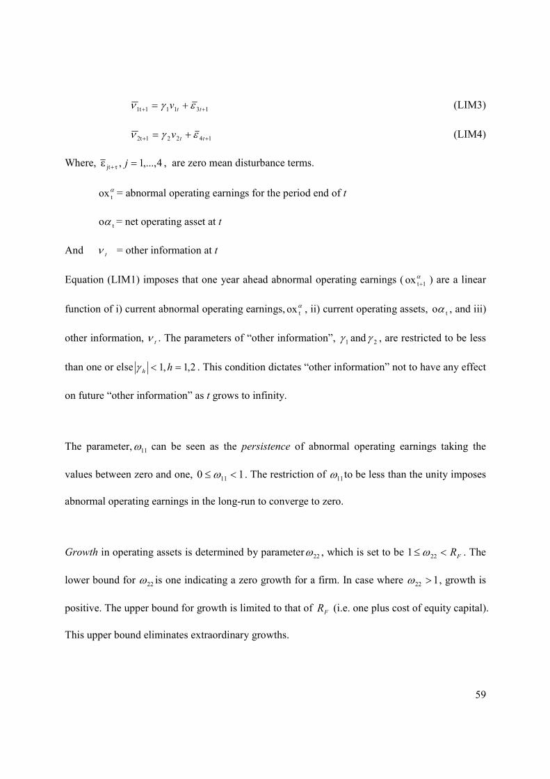
59

131111t ++ += ttv εγν (LIM3)

142212t ++ += ttv εγν (LIM4)

Where, 4,...,1,ε τjt =+ j , are zero mean disturbance terms.

αtox = abnormal operating earnings for the period end of t

toα = net operating asset at t

And tν = other information at t

Equation (LIM1) imposes that one year ahead abnormal operating earnings ( α1tox + ) are a linear

function of i) current abnormal operating earnings, αtox , ii) current operating assets, toα , and iii)

other information, tν . The parameters of “other information”, 1γ and 2γ , are restricted to be less

than one or else 2,1,1 =< hhγ . This condition dictates “other information” not to have any effect

on future “other information” as t grows to infinity.

The parameter, 11ω can be seen as the persistence of abnormal operating earnings taking the

values between zero and one, 10 11 <≤ ω . The restriction of 11ω to be less than the unity imposes

abnormal operating earnings in the long-run to converge to zero.

Growth in operating assets is determined by parameter 22ω , which is set to be FR<≤ 221 ω . The

lower bound for 22ω is one indicating a zero growth for a firm. In case where 122 >ω , growth is

positive. The upper bound for growth is limited to that of FR (i.e. one plus cost of equity capital).

This upper bound eliminates extraordinary growths.

60

The final parameter, 12ω , is related to unbiased versus conservative accounting. As discussed

above (see, Ohlson (1995) model), Feltham & Ohlson (1995) incorporated conservative

accounting in their model. Thus, a positive 12ω indicates conservative accounting whilst a zero

12ω relates to unbiased accounting. Setting 012 =ω , LIM1 becomes similar to Equation (ID1) of

Ohlson (1995) model which is built on “perfect accounting”. Hence, the restriction for the

parameter 12ω is 012 ≥ω . Based on the analysis above, Feltham & Ohlson (1995) derive a linear

valuation function as follows:

tt

a

ttt oaoxbvP βναα +++= 21 (3.9)

Where, ttt oafabv +=

11

111 ω

ωα

−=

FR

( )( )1122

122 ωω

ω−−

=FF

F

RR

Ra

( )( )( ) ( )

−−−==

2

2

111

21 ,,γ

αγω

βββFFF

F

RRR

R

Comparing Ohlson (1995) model, Equation (3.8), and Feltham & Ohlson (1995) model, Equation

(3.9), they differ as of the toa variable. A positive parameter for toa , ( )02 >α , is the correction

for the understatement of book value of equity due to conservative accounting. When 02 =α ,

Equation (3.9) becomes identical to Ohlson (1995) model (see, Equation (3.8)), indicating

unbiased accounting.

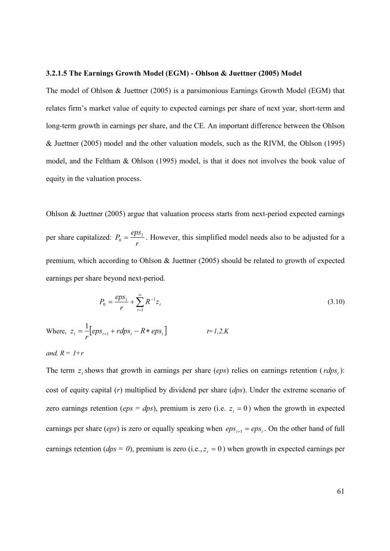
61

3.2.1.5 The Earnings Growth Model (EGM) - Ohlson & Juettner (2005) Model

The model of Ohlson & Juettner (2005) is a parsimonious Earnings Growth Model (EGM) that

relates firm’s market value of equity to expected earnings per share of next year, short-term and

long-term growth in earnings per share, and the CE. An important difference between the Ohlson

& Juettner (2005) model and the other valuation models, such as the RIVM, the Ohlson (1995)

model, and the Feltham & Ohlson (1995) model, is that it does not involves the book value of

equity in the valuation process.

Ohlson & Juettner (2005) argue that valuation process starts from next-period expected earnings

per share capitalized: r

epsP 1

0 = . However, this simplified model needs also to be adjusted for a

premium, which according to Ohlson & Juettner (2005) should be related to growth of expected

earnings per share beyond next-period.

t

t

zRr

epsP ∑

∞

=

−+=1

110 (3.10)

Where, [ ]tttt epsRrdpsepsr

z ∗−+= +1

1 t=1,2,K

and, R = 1+r

The term tz shows that growth in earnings per share (eps) relies on earnings retention ( trdps ):

cost of equity capital (r) multiplied by dividend per share (dps). Under the extreme scenario of

zero earnings retention (eps = dps), premium is zero (i.e. 0=tz ) when the growth in expected

earnings per share (eps) is zero or equally speaking when tt epseps =+1 . On the other hand of full

earnings retention (dps = 0), premium is zero (i.e., 0=tz ) when growth in expected earnings per

62

share equals r ( reps

epseps

t

tt =−+1 ). The case of zero premium ( 0=tz ) in Equation (3.10) leads to

normal earnings performance, withr

epsP 1

0 = . However, in case of zt>0, the model implies

superior earnings performance. Ohlson & Juettner (2005) impose tz to follow an AR (1) process

as shown below:

tt zz ∗=+ γ1 , t=1, 2, K (3.11)

Where, R<≤ γ1 and 01 >z

The growth rate γ is restricted to be equal or greater than the unity. Ohlson & Juettner (2005)

argue that a growth rate of less than one is implausible given conservative accounting. Note that

when 1<γ expected earnings per share (eps) performances become normal as t grows to infinity.

Assuming a fixed growth rate for z , equation (3.10) is restated as:

γ−+=

R

z

r

epsP 11

0 (3.12)

Where, [ ]112

1

1 epsRrdpsepsrz ∗−+= −

Equation (3.12) can be seen as a generalization of the Gordon Growth Model (see, Section

3.2.1.1). Introducing a measure of short-term growth in equation (3.12) such

as rgreps

dpsr

eps

epsepsg −≡−

+

−≡ 2

1

1

1

122

ˆ , Ohlson & Juettner (2005) derive their valuation

formula as follows:

( )( )1

11ˆ1

1 22

1

0

−−

−−∗=

−

+=γγ

γ r

g

rR

g

reps

P (3.13)

Solved as for the cost of equity capital, r:

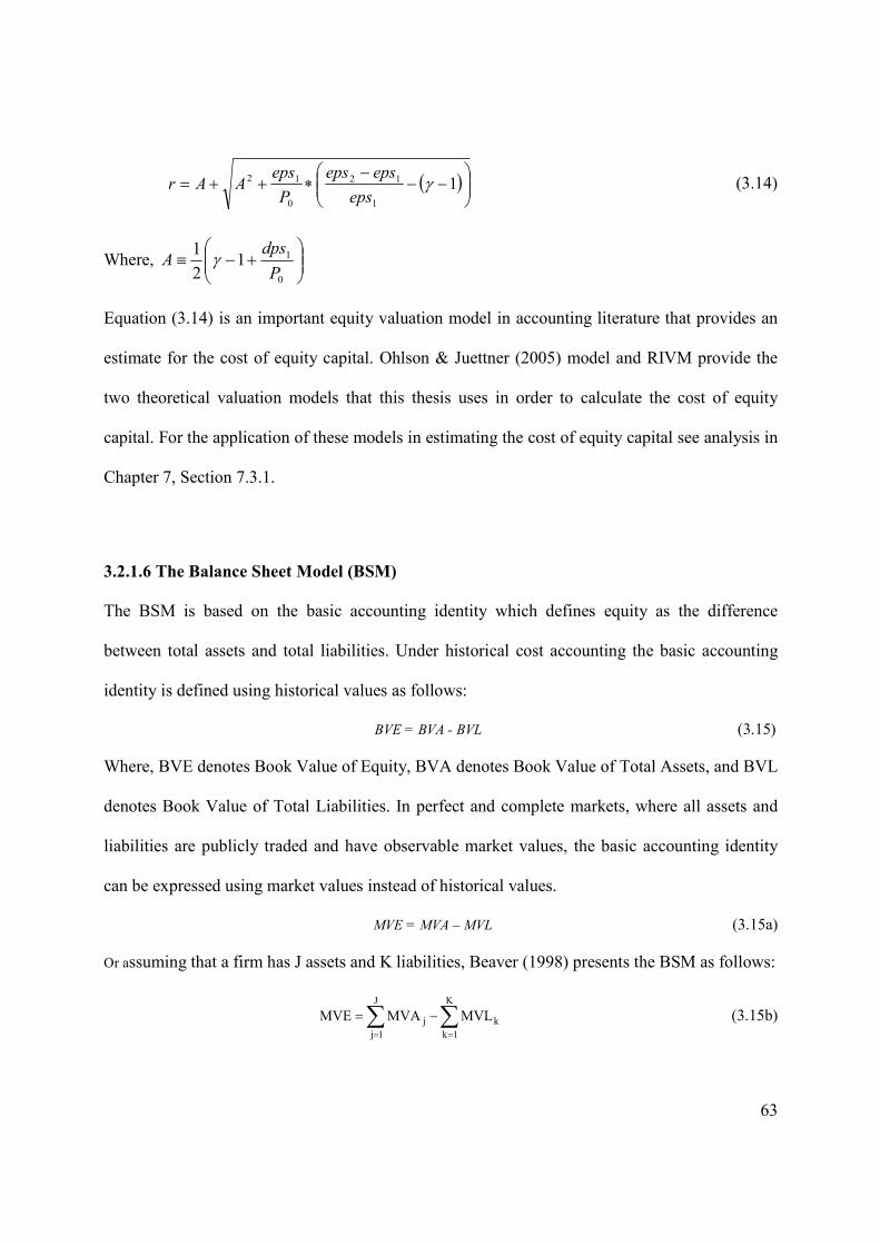
63

( )

−−

−∗++= 1

1

12

0

12 γeps

epseps

P

epsAAr (3.14)

Where,

+−≡

0

112

1

P

dpsA γ

Equation (3.14) is an important equity valuation model in accounting literature that provides an

estimate for the cost of equity capital. Ohlson & Juettner (2005) model and RIVM provide the

two theoretical valuation models that this thesis uses in order to calculate the cost of equity

capital. For the application of these models in estimating the cost of equity capital see analysis in

Chapter 7, Section 7.3.1.

3.2.1.6 The Balance Sheet Model (BSM)

The BSM is based on the basic accounting identity which defines equity as the difference

between total assets and total liabilities. Under historical cost accounting the basic accounting

identity is defined using historical values as follows:

BVE = BVA - BVL (3.15)

Where, BVE denotes Book Value of Equity, BVA denotes Book Value of Total Assets, and BVL

denotes Book Value of Total Liabilities. In perfect and complete markets, where all assets and

liabilities are publicly traded and have observable market values, the basic accounting identity

can be expressed using market values instead of historical values.

MVE = MVA – MVL (3.15a)

Or assuming that a firm has J assets and K liabilities, Beaver (1998) presents the BSM as follows:

∑ ∑= =

−=J

1j

K

1k

kj MVLMVAMVE (3.15b)

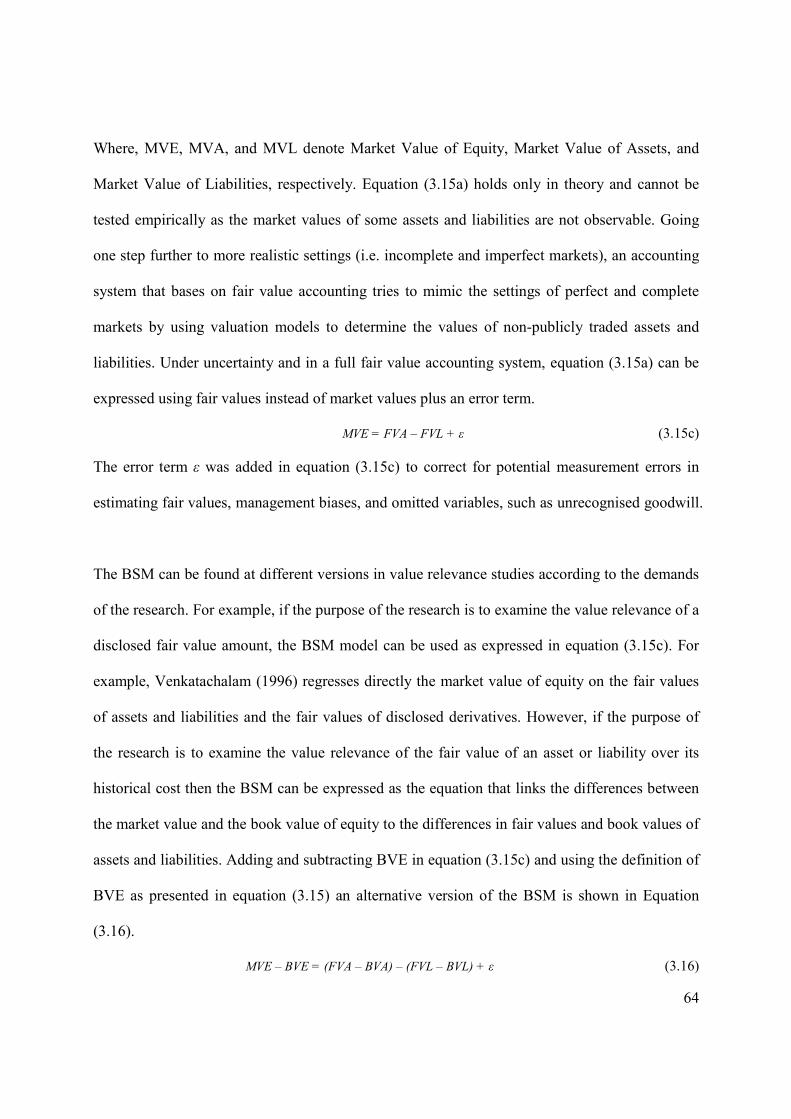
64

Where, MVE, MVA, and MVL denote Market Value of Equity, Market Value of Assets, and

Market Value of Liabilities, respectively. Equation (3.15a) holds only in theory and cannot be

tested empirically as the market values of some assets and liabilities are not observable. Going

one step further to more realistic settings (i.e. incomplete and imperfect markets), an accounting

system that bases on fair value accounting tries to mimic the settings of perfect and complete

markets by using valuation models to determine the values of non-publicly traded assets and

liabilities. Under uncertainty and in a full fair value accounting system, equation (3.15a) can be

expressed using fair values instead of market values plus an error term.

MVE = FVA – FVL + ε (3.15c)

The error term ε was added in equation (3.15c) to correct for potential measurement errors in

estimating fair values, management biases, and omitted variables, such as unrecognised goodwill.

The BSM can be found at different versions in value relevance studies according to the demands

of the research. For example, if the purpose of the research is to examine the value relevance of a

disclosed fair value amount, the BSM model can be used as expressed in equation (3.15c). For

example, Venkatachalam (1996) regresses directly the market value of equity on the fair values

of assets and liabilities and the fair values of disclosed derivatives. However, if the purpose of

the research is to examine the value relevance of the fair value of an asset or liability over its

historical cost then the BSM can be expressed as the equation that links the differences between

the market value and the book value of equity to the differences in fair values and book values of

assets and liabilities. Adding and subtracting BVE in equation (3.15c) and using the definition of

BVE as presented in equation (3.15) an alternative version of the BSM is shown in Equation

(3.16).

MVE – BVE = (FVA – BVA) – (FVL – BVL) + ε (3.16)

65

Equation (3.16) is a widely used theoretical model in the value relevance literature (e.g., Barth et

al., 1996; Eccher et al., 1996; Nelson, 1996; Park et al., 1999; Petroni & Wahlen, 1995). It

examines the extent to which the differences between fair values and book values of assets and

liabilities explain cross-sectionally the discrepancy between the market value and the book value

of equity. The rationale of this model (Equation 3.16) is that as long as the fair values of assets

and liabilities are measures of current values then any material difference between fair values

and historical costs should explain the excess of market value of equity over the book value of

equity.

As discussed in Section 3.2.1.1, Barker (2001) suggests that each valuation model should be

reconciled with the fundamental valuation model, the DDM, in order to be theoretically

consistent. Barth (p. 12, 2000) suggests that the,

‘asset and liability values are the present value of the expected dividends, or cash flows, associated with the underlying rights and obligations’

This statement implies a direct link between the two models, the DDM and the BSM. The

following two equations demonstrate this link as they show that the fair values of assets

(Equation 3.17) and liabilities (Equation 3.18) can be alternatively viewed as the discounted

future claims and obligations, respectively.

( )[ ]( )∑∑

=

∞

= +=

i

i tn

it

k

ACFEFVA

1 1 1

(3.17)

( )[ ]( )∑∑

=

∞

= +=

J

J tn

Jt

k

LCFEFVL

1 1 1

(3.18)

Where, ( )[ ]it ACFE and ( )[ ]Jt LCFE refer to the Expected Cash Flows of an Asset i and

Expected Cash Flows of a Liability J, respectively and k is the prevailing interest rate.

66

3.2.2 Cost of equity capital

The discussion above demonstrated the importance of the CE in the equity valuation theory. This

section discusses the standard approaches in the literature to calculate the CE. The CE is an

unobservable measure that investors require as a return when they invest on a firm. The fact that

it is unobservable requires its estimation. Two streams can be found in the literature to estimate

the CE. The first stream uses asset pricing models, such as the CAPM, and the second stream

uses equity valuation models, such as the RIVM.

Since the development of the CAPM in the 1960s, finance literature recommended the use of an

asset pricing model (e.g. the CAPM or the three-factor model of Fama & French, 1993, 1995,

1996) in estimating the equity risk premium (i.e. the CE)7. Asset pricing models have their origin

to the seminal work of Markowitz (1959) suggesting that individuals base their investment

decisions on two statistical measures, the mean, and the variance. Under the mean-variance

analysis, as it is alternatively known in the finance literature, rational investors seek to select

investment portfolios that maximize their expected returns while at the same time minimize the

variance of returns.

Building on the mean-variance analysis, Sharpe (1964) and Lintner (1965) developed the CAPM

which provided the first theoretical approach on how to quantify the risk and return of capital

assets. Based on two assumptions that all investors have homogenous expectations about the

distribution of assets’ expected returns, and the existence of borrowing and lending at a risk-free

rate of interest, CAPM defines the expected return of an asset as a function of the risk-free

7 The equity risk premium is defined as the excess required rate of return over the risk-free rate usually the interest

rate of the 10-years government US bonds.

67

interest rate, fR plus a risk premium, the covariance of asset’s return, ( )iE R , with the return of

the market portfolio, ( )ME R ,

( ) [ ( ) ]i f iM M fE R R E R Rb= + -

Where, 2

( , )

( )

i MiM

M

Cov R R

Rb

s=

Fama & French (1993, 1995) provided empirical evidence that size and book-to-market equity

(the ratio of book value of equity to market value of equity) can further explain the cross-section

variations of expected returns incrementally to the market risk. The three-factor model has been

used by both empirical research and practitioners as an alternative to the CAPM in order to

provide estimates of the CE. A forth factor usually added to the three-factor model is the

‘momentum effect’ which means that stocks that performed well relative to the market, tend to

continue to outperform in the future and vice versa, stocks that underperformed in the near past

tend to underperform in the future (Carhart, 1997; Jegadeesh & Titman, 1993).

However, later empirical evidence suggests that using the CAPM, or the Fama & French model,

is a flawed way of estimating the equity risk premium (Claus & Thomas, 2001; Fama & French,

2004). A major criticism is that they are based on historical data (i.e. realised returns). Thus, later

studies turned to a more dynamic approach in estimating the CE using forward looking data,

such as forecasted analysts’ earnings per share (Claus & Thomas, 2001; Easton et al., 2002;

Gebhardt et al., 2001; Gode & Mohanram, 2003; Ohlson & Juettner, 2005). These studies are

based on equity valuation theory and specifically on the RIVM and the EGM, discussed in

Sections 3.2.1.2 and 3.2.1.5, respectively.

68

Under the RIVM, the CE is the model-implied required rate of return which can be seen

alternatively as the internal rate of return (IRR) that equates the current share price of a firm, to

the current book value per share and the discounted expected abnormal earnings.

The EGM, as developed by Ohlson-Juettner (2005), is a parsimonious valuation model that

relates share price to the one-year ahead and two-year ahead earnings per share, the forthcoming

dividend per share, a perpetual growth rate (γ), and a short-term growth that is assumed to decay

asymptotically to the perpetual growth rate (γ). Contrary to the RIVM, the Ohlson-Juettner (2005)

model needs no estimates of the forecasted book values per share and does not requires data for

the forecasted earnings per share beyond the second year ahead.

Hence, given the limitations of the CAPM, this thesis focuses on the second stream of research to

estimate the CE, which uses forecasted data instead of historical data. In total, four models are

used to estimate the CE. The first two models are based on the RIVM and are the Gebhardt et al.

(2001) model and the Claus & Thomas (2001) model. The other two models are based on the

EGM and are the Gode & Mohanram (2003) model and the Easton (2004) model. These models

are discussed extensively in the methodology chapter of the cost of equity capital (see, Chapter

7). The fact that all of the four models above are based on subjective assumptions (e.g. expected

growth in earnings) makes the calculation of the CE sensitive to different inputs. Thus, given that

none of these four models is proved in practice to be superior relative to the others, the average

CE is also used in the empirical analysis. The next section shows the link between CE and

accounting standards.

69

3.3 CE and accounting standards

The purpose of this section is to explain the relationship between CE and accounting standards.

The section is separated into two sections. The first section explores how increased disclosure

relates to the CE. Most of theoretical discussion predicts that increased disclosure and more

quality in financial reporting results in lower CE. The second section provides some views that

one set of accounting standards, such as the IFRS, may result in lower CE. Diverse accounting

standards result in more adjustment costs when investors compare financial statements prepared

under different accounting rules.

3.3.1 Increased disclosure and CE

The notion that high quality accounting standards and increased disclosure decrease CE and

hence increase share prices, ceteris paribus, is a dominant theme in the accounting literature

(Ball, 2006; Levitt, 1998). As early as 1950s, Horngren (1957, p. 598) suggested that:

‘It is probable that the analyst would be better able to make intelligent decisions concerning securities if he should receive corporate information in bigger and better quantities and qualities’. He also added that, ‘Analysts generally will be more interested in firms that disclose as opposed to those which do not’. Horngren (1957, p. 600). The argument of Horngren (1957) above implies that increased disclosure constitutes a positive

signal for analysts in particular, and investors in general. Well-informed investors experience

less uncertainty in their investment decision process and as a consequence, apply a relatively

lower CE to those firms that disclose more. A relatively lower CE is translated into a relatively

higher share price for firms with increased disclosure. Two streams of research exist in the

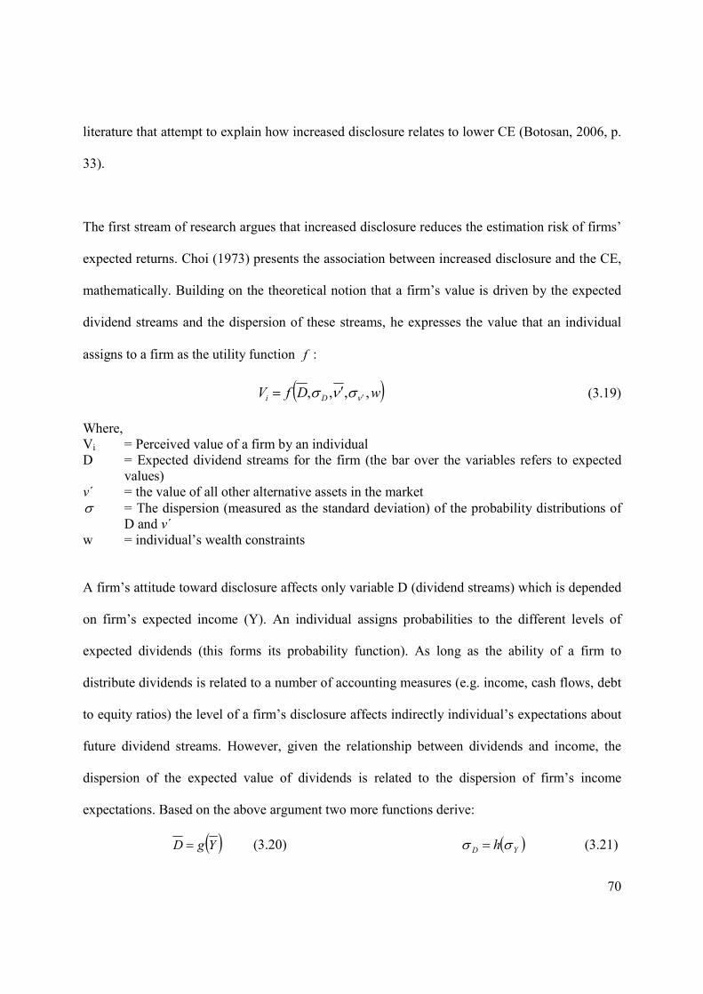
70

literature that attempt to explain how increased disclosure relates to lower CE (Botosan, 2006, p.

33).

The first stream of research argues that increased disclosure reduces the estimation risk of firms’

expected returns. Choi (1973) presents the association between increased disclosure and the CE,

mathematically. Building on the theoretical notion that a firm’s value is driven by the expected

dividend streams and the dispersion of these streams, he expresses the value that an individual

assigns to a firm as the utility function f :

( )wDfV Di ,,,, νσνσ ′′= (3.19)

Where, Vi = Perceived value of a firm by an individual D = Expected dividend streams for the firm (the bar over the variables refers to expected

values) v´ = the value of all other alternative assets in the market

σ = The dispersion (measured as the standard deviation) of the probability distributions of D and v´

w = individual’s wealth constraints

A firm’s attitude toward disclosure affects only variable D (dividend streams) which is depended

on firm’s expected income (Y). An individual assigns probabilities to the different levels of

expected dividends (this forms its probability function). As long as the ability of a firm to

distribute dividends is related to a number of accounting measures (e.g. income, cash flows, debt

to equity ratios) the level of a firm’s disclosure affects indirectly individual’s expectations about

future dividend streams. However, given the relationship between dividends and income, the

dispersion of the expected value of dividends is related to the dispersion of firm’s income

expectations. Based on the above argument two more functions derive:

( )YgD = (3.20) ( )YD h σσ = (3.21)

71

Individuals form their expectations about a firm’s income, Y, based on a set of information, such

as past data and future expectations regarding a firm (e.g. accounting data), data on the related

industry, and macroeconomic factors. Thus, the income distribution function of an individual j

for a firm i in an industry N is conditional on the available information to this individual and can

be expressed mathematically as, ( )iNj ItY = . Choi (1973) makes the assumption that the higher

the level of information iNj I , the better the firm and the industry performs in total8. He also

argues that although the expectations of each individual separately for a firm’s accounting

variables are poor estimates of ‘true’ value, taking the expectations of individuals in total, they

are quite unbiased estimates of the long-term ‘true’ value. Equations (3.19) to (3.21) together

with equation ( )iNj ItY = are aggregated in a single equation (3.22). Taking the differential

calculus of equation (5.22) with respect to I and Iσ , equations (3.23) and (3.24) derive

respectively.

( )[ ]

= ItgfVi (3.22)

IdI

Y

Y

D

D

VdV i

i

∂∂

∂∂

∂∂

= (3.23)

I

I

Y

Y

D

D

ii d

VdV σ

σσ

σσ

σ

∂∂

∂∂

∂∂

= (3.24)

Interpreting equations (3.23) and (3.24), Choi (1973) argues that increased disclosure affect a

firm’s value not by changing the mean expectations of the individuals, which assumed to be

unbiased estimates of the true values and thus 0=∆Ι i , but through the reduction in the

8 Choi (1973) explains that an increase in earnings or/and a decrease in debt to equity ratio are signals of good

performance resulting in both cases in an increase of the level ofiNj I . This is based on the assumption that firms

that perform well are more likely to disclose more, in order to communicate the good ‘news’ to the market.

72

dispersion, Iσ , regarding these expectations. Thus, individuals become less uncertain about the

future expectations of accounting variables. Given the fact that: i) any firm’s value at any point

in time incorporates the mean expectations of all investors, and ii) increased disclosure reduces

the dispersion of these expectations and hence uncertainty, and as a consequence CE is reduced

and share price increases.

In another study, Barry & Brown (1985) provide an example of two securities (A and B) in order

to explain that increased disclosure matters when investors choose between competing

investments. They first assume that the two securities, A and B, have identical estimates of

expected returns and variances, but estimates of security A are based on twenty quarterly

observations, whilst estimates of B are based on only four quarterly observations. Barry &

Brown (1985) argue that in a Bayesian framework the dispersion in the distribution of future

returns will be higher for security B and lower for security A. Thus, investors would prefer to

invest in firm A with the lower estimation risk. Coles et al. (1995) support also the view that

increased disclosure reduces the estimation risk that investors face when estimate payoff

distributions. They argue that investors have more information for some firms which results in

lower beta (i.e. CE) and higher share price.

The second stream of research argues that increased disclosure decreases information

asymmetries between managers and shareholders, which increases securities’ liquidity, which in

return reduces the CE. Amihud & Mendelson (1986) argue that higher bid-ask spreads result in

higher transaction costs for investors who require higher returns. This fact increases firms’ CE.

Amihud & Mendelson (1986) also argue that firms with high bid-ask spreads have incentives to

73

increase the liquidity of the issued securities through information disclosure. In another study,

Diamond & Verrecchia (1991) provide evidence that the CE decreases when the liquidity of

share prices increases due to higher levels of disclosure. They explain that improvement in

liquidity attracts large traders who increase demand for firm’s securities and thus increase share

price and reduce CE. Finally, Easley & O’hara (2004) argued that investors demand higher

return for firms with greater private information than public information. They suggest that:

‘firms can influence their cost of capital by affecting the precision and quantity of information available to investors. This can be accomplished by a firm’s selection of its accounting standards, as well as through its corporate disclosure policies’ Easley & O’hara (2004, p. 1578).

Uninformed investors face higher uncertainty and thus demand higher return for firms with

higher private information. However, if a firm starts to disclose more information to the market

this will increase demand for its shares, which in return will increase liquidity. Finally, more

public information is related to lower information asymmetries which decrease firm’s CE.

However, increased disclosures may not always result in lower CE for all firms. It is likely that

disclosing more information to the financial markets will cause more variability in share prices,

especially when the disclosed information reveals additional risk for these firms. A recent

example was the financial crisis of 2008, where a number of banks that were disclosing the

negative changes in the fair values of their financial instruments resulted in high share price

variability around the date of the disclosures. Hence, even that the theory suggests that increased

disclosure is better than poor disclosure this is may not always be the case under certain

conditions (e.g. financial crises).

74

3.3.2 Uniformity of accounting standards and CE

The adoption of one set of accounting standards by a number of countries that previously applied

diverse accounting standards may reduce CE. Investors when they have to select between two

equity investments usually compare (among other things) the financial statements of these firms.

If the firms follow different accounting standards, investors need to make adjustments in order to

make the results comparable. This procedure demands an in-depth knowledge of the different

accounting rules which incurs additional costs for investors, such as to educate themselves in

order to interpret financial statements prepared under different accounting standards.

There are views in accounting practice and academic literature that one set of accounting

standards may lead to a lower CE. For example, Sir David Tweedie, the then Chairman of IASB,

argued in 2004 in his speech, before the Committee on Banking, Housing and Urban Affairs of

the United States Senate that:

‘A single set of international standards will enhance comparability of financial information and should make the allocation of capital across borders more efficient The development and

acceptance of international standards should also reduce compliance costs for corporations and

improve consistency in audit quality.’9

This view is shared by Ball (2006, p. 11) who suggests that investors will be benefitted if many

countries adopt the IFRS as this will reduce the adjustment costs for making financial statements

comparable. Several other academic studies support this proposition. For example, Armstrong et

al. (2010, p. 32) argued that,

‘Investors also might have believed that application of a common set of standards would have convergence benefits, such as lowering the costs of comparing firms’ financial position and performance across countries…’.

9 Available from: http://www.iasplus.com/resource/040909tweedietestimony.pdf [Accessed 19 January 2011].

75

Moreover, Hail et al. (2010, p. 358) argued that comparability also increases liquidity as

investors can distinguish between less and more profitable firms. As explained above, this

increased liquidity results in lower information asymmetries and as a consequence lower CE.

Ray (2010) also examined the costs and benefits of uniform accounting standards based on a

neoclassical approach. He argues that regulators (e.g. IASB) aim to provide accounting standards

that maximize social welfare. Uniform accounting standards improve social welfare if variation

between firms is low. Firms with small differences (e.g. in size) have lower compliance costs as

standard-setters produce accounting standards that fit better to the ‘average’ firm. On the other

hand, if differences between firms are large, then multiple accounting standards serve better the

needs of firms as they reduce compliance costs, and as a consequence promote social welfare.

Ray (2010) also explains that when differences between investors are large then uniform

accounting standards are those that increase social welfare because they draw more investors in

capital markets providing more liquidity. Investors experience costs of interpreting diverse

accounting standards and making the necessary adjustments. Uniform accounting standards aid

investors to compare investment opportunities in an economy and to allocate capital efficiently.

Efficient capital allocation reduces the CE. Hence, Ray (2010) concludes that standard-setters

need to trade-off the costs and benefits of applying uniform accounting standards as opposed to

diverse accounting standards.

However, despite the benefits of one set of accounting standards (under certain assumptions,

see, Ray, 2010), Zeff (2007) argues that genuine comparability is still difficult to be achieved

(under the IFRS) due to cultural differences between countries. Such differences are related to i)

business and financial culture, ii) accounting culture, iii) auditing culture, and iv) regulatory

76

culture. Thus, whether the adoption of IFRS lead to higher comparability between the financial

statements of firms, which prepare their accounts under different accounting standards, is an

empirical question.

3.4 A critical view of value relevance research

Value relevance research uses empirical models to examine the relevance and reliability of any

accounting number published in financial statements. Beaver (2002, p. 462) explains that,

‘the theoretical foundation of value relevance studies is a combination of a valuation theory plus contextual accounting arguments that allow researchers to predict how accounting variables relate to the market value of equity’.

Thus, Beaver (2002) suggests that value relevance research is based on two elements: valuation

theory (described above in Section 3.2) and contextual accounting arguments which set the

accounting questions that researchers want to explore. For example, a contextual accounting

argument of this thesis is the first research question presented in Section 1.2 that examines

whether fair value estimates under IFRS for the financial instruments of European commercial

banks are value relevant incrementally to their book values.

Proponents of value relevance argue that the results of value relevance research can inform

standard setting as it is a way to operationalize the qualitative characteristics of accounting

information, the relevance and reliability (Barth et al., 2001). Barth (2007, p. 8) observes that,

‘when applying the Framework to measurement questions, the IASB focuses on determining which measurement basis best meets the objective of financial reporting, the elements definitions, and the qualitative characteristics of accounting information’.

77

Thus, Barth (2007, p. 13) argues that value relevance studies can inform standard setters on the

extent various measurement bases comply with the qualitative characteristics of relevance and

reliability (i.e. faithful representation), as stated in the IASB’s Conceptual Framework (IASB,

2010).

However, other studies take an opposite view. For example, Holthausen & Watts (2001, p. 4)

argue that without an underlying descriptive theory of accounting and standard setting, value

relevance research has limited implications for standard setting. They also suggest that the

associations between accounting numbers and market values, that value relevance studies report,

are of little interest to standard setters. Another criticism of value relevance research is that it

focuses only on one group of users of financial statements; the investors, who use accounting

information in their investment decision making process. However, accounting information is

also be used for contracting purposes (Watts & Zimmerman, 1986) and this is ignored by value

relevance research. However, Barth et al. (2001) suggest that,

‘Although financial statements have a variety of applications beyond equity investment, e.g., management compensation and debt contracts, the possible contracting uses of financial statements in no way diminish the importance of value relevance research, which focuses on equity investment’.

Thus, based on the argument above, financial reporting serves different objectives and users of

financial statements. The fact that value relevance research focuses only on a single group of

users, the investors, it does not mean that financial reporting can not serve other purposes such as

contracting purposes (i.e. debt covenants). The methodology of this thesis adopts the investor

point of view as the objective of financial reporting. This decision does not diminish the

78

importance of financial statements for contracting purposes which is also another core objective

of financial reporting.

3.5 Conclusion

This chapter discussed the equity valuation theory which provides the theoretical framework for

the empirical part of the thesis, i.e., value relevance and the economic consequence tests. Value

relevance studies underpin the development of their empirical models on equity valuation theory

as otherwise these models would have been regarded as ad hoc constructs. Equity valuation

theory also provides the theoretical models for estimating the cost of equity capital which is

prerequisite for the economic consequence part.

The valuation models presented are: i) the DDM which is the neoclassical approach to valuation,

ii) the RIVM that uses accounting numbers to derive equity’s value, iii) the Ohlson (1995) model

which builds on the RIVM by incorporating linear information dynamics, iv) the Feltham &

Ohlson (1995) model that extends Ohlson (1995) model to incorporate conservative accounting,

v) the Ohlson & Juettner (2005) model which is a an abnormal earnings growth valuation model,

and vi) the BSM that relates equity value to the difference between assets and liabilities’ values

(i.e. the basic accounting identity).

As stated in the introduction, the interest of this thesis is to examine whether fair value estimates

of banks’ assets and liabilities are value relevant incrementally to their book values. Thus, for the

value relevance tests of this thesis, the model that provides the link between accounting numbers

and market values is the BSM. The advantage of the BSM model over the other valuation models

79

(e.g. RIVM) is that it provides a direct link between the values of assets and liabilities and the

market value of equity.

Equity valuation theory also provides the theoretical background for estimating the CE, a vital

measure for the economic consequence test. In particular, this thesis uses four methods of

estimating the CE, which are the most common in accounting literature (Daske et al., 2008). Two

of the models are based on the RIVM and are the Gebhardt et al. (2001) method and the Claus &

Thomas (2001) method. The other two models are based on the EGM and are the Gode &

Mohanram (2003) method and the Easton (2004) method10. The advantage of these models over

other models, such as the CAPM is that they use forward looking data (e.g. expected earnings)

instead of historical data.

The chapter also analyzed the relationship between CE and accounting standards. In summary,

theoretical studies conclude that increased disclosure reduces CE. Choi (1973) has shown

mathematically that the CE reduces when the dispersion of the expectations on firms accounting

variables decreases. Amihud & Mendelson (1986) and Diamond & Verrecchia (1991) found that

the CE is reduced when increasing the liquidity of share prices and Easley & O’hara (2004)

argue that firms can reduce CE if they choose to provide more public information than private

information. Moreover, the adoption of IFRS (which for most countries is a commitment to

increased disclosure and to more quality in financial reporting) can reduce CE through better

comparability of financial statements across countries. This is mainly because investors will

eliminate the necessary adjustments in order to make firms’ accounts comparable (Ball, 2006;

Armstrong et al., 2010). The benefits of uniform accounting standards will be higher the lower is

the variation between firms (Ray, 2010).

10 These four models are discusses in details in Chapter 7, the methodology chapter for the cost of equity test.

80

Finally, the chapter presented a critical view of the value relevance research. Advocates of the

value relevance research argue that this type of research can provide valuable inputs to standard

setters, given that it is a way to operationalize relevance and reliability (i.e. faithful

representation), two qualitative characteristics stated in IASB’s and FASB’s conceptual

frameworks (Barth et al., 2001). On the other hand, other researchers believe that value relevance

cannot inform standard setters in the absence of an underlying descriptive theory of accounting

and standard setting Holthausen & Watts (2001).

Having analysed extensively the equity valuation theory which underpins both the value

relevance and the economic consequence tests, the next two chapters review the empirical

studies of the value relevance literature (Chapter 4) and the empirical studies relating to the

economic consequence part (Chapter 5).

81

Chapter 4: Review of Value Relevance Empirical Studies

4.1 Introduction

So far this thesis has explored the theoretical framework of the study, the equity valuation theory

(see, Chapter 3). Several value relevance studies have used this framework to empirically test the

relevance and reliability of accounting numbers either recognised in the financial statements or

disclosed in the notes. In particular, the value relevance literature attempts to operationalize the

standard setters’ qualitative characteristics of relevance and reliability by using empirical models

underpinned by the equity valuation theory (Barth et al., 2001).

The purpose of this chapter is to analyse the empirical findings of the value relevance literature.

Value relevance studies adopt the view that investors are the core users of financial statements

and, therefore, they use econometric techniques to provide evidence on the relationship between

accounting numbers and share prices. Barth (2000, p. 16) defines value relevance as the extent to

which ‘…the accounting amount is associated with some measure of value e.g. share prices’. In

another study of Eccher et al. (p. 80, 1996), value relevance is defined ‘…in terms of the

association of supplementary fair value disclosures with share prices’. Although value relevance

studies test several accounting numbers in the financial statements (e.g. net income), this thesis is

particularly focused on the value relevance of fair value measures. Value relevance studies

conclude that the measurement method (e.g. fair value or amortized cost) that correlates the most

with share prices is the most relevant to investors (AAA FASC, 1998).

Due to the fact that this study deals with banks, the review of empirical studies is categorised

into two groups: banking and non-banking. Section 4.2 presents the empirical studies on banks.

82

The analysis distinguishes further between US and non-US studies. This distinction is made

because US studies dominated the value relevance literature, whilst non-US studies and in

particular, studies on IFRS are not in a plethora. All of the studies, however, both US and non-

US relate to financial instruments. Section 4.3 discusses the non-banking literature, which covers

industries such as industrial firms, mutual funds, property-liability insurers, software firms,

investment property firms. The analysis is again presented separately for US and non-US studies.

The literature on non-banks involves not only financial instruments, but also intangible and

tangible assets. Finally, Section 4.4 concludes.

4.2 Empirical Studies on Banks

The value relevance literature on banks is mainly related to financial instruments. This is not

surprising given that financial instruments constitute the majority of bank’s assets and liabilities.

4.2.1 The US literature

As discussed in Chapter 2, Section 2.2.6, SFAS 107 was the first US standard which required the

disclosure of the fair values of all financial instruments in the notes of the financial statements.

Therefore, studies before SFAS No. 107 examined fair values in a period where banks were

disclosing voluntarily fair values in the notes of financial statements. The discussion of these

studies is in Section 4.2.1.1. Section 4.2.1.2 provides the findings under SFAS No. 107 and

under the derivative standards, SFAS Nos. 109 and 133. SFAS No. 115 required the

classification of equity and debt securities in three categories, namely: held-to-maturity, trading

83

assets, and available-for-sale securities. These studies are analysed in Section 4.2.1.3. Finally,

Section 4.2.1.4 discusses recent studies that relate to the requirements of SFAS No. 157.

4.2.1.1 Evidence before SFAS No. 107

Two early studies of Barth (1994) and Ahmed & Takeda (1995) provide some first evidence on

the fair values of investment securities. The samples of these studies cover periods before 1992,

the year when SFAS No. 107 became effective. Before this standard, US banks voluntarily

disclosed the fair values of investment securities.

Barth (1994) provides evidence on the value relevance of investment securities’ fair values and

their related gains and losses. Using data from 1971 – 1990 for US banks she sheds some light

on the argument surrounding the merits of fair value accounting over historical cost accounting.

Specifically, Barth examines two research questions, namely: i) whether investment securities’

fair values are associated with share prices incrementally to historical costs, and ii) whether fair

value gains and losses, resulted by changes in investment securities’ fair values, are associated

more with changes in share prices (returns) than historical costs. Her methodology for the value

relevance of investment securities’ fair values is based on the BSM described in Chapter 3.

Including in a single model the two values of investment securities (the recognised historical

values and disclosed fair values) and the book value of equity before investment securities, she

reports a higher coefficient for investment securities’ fair values, indicating incremental

explanatory power to historical costs. On the other hand, using an earnings capitalisation model

no evidence is provided for the fair values’ gains and losses of investment securities.

84

One should expect that as long as investment securities’ fair values have incremental explanatory

power, then fair values’ gains and losses (which are the changes in investment securities’ fair

values) should also have incremental explanatory power. Barth (1994) provides two

interpretations. i) Estimation errors in investment securities’ fair values are relative small when

considered separately for each year. However, taking together two years to calculate securities’

gains and losses this makes the aggregated estimation errors larger, affecting the results for the

gains and losses. ii) Correlated omitted gains and losses from assets and liabilities that are not

taking into account by the model (e.g. non-investment securities), could have hedged the

investment securities’ fair value gains and losses making them insignificant.

Contrary to Barth (1994) who gives support to the first interpretation, Ahmed & Takeda (1995)

provide evidence for the second interpretation. Specifically, they found that failing to control in

the model for net assets’ gains and losses of non-investment securities (due to interest rate

changes), can bias the coefficient of the changes in unrealised gains and losses of investment

securities.

Another study before SFAS No. 107 is that of Riffe (1997). This study provides evidence on the

valuation implication of the notional amounts of derivatives in a period where the US GAAP did

not require the disclosure of fair values of derivatives. Banks were disclosing from 1986 the

notional amounts of all off-balance sheet instruments in the Y-9 reports as required by Federal

Reserve. Later on, SFAS No. 105 also required banks to disclosure the notional amounts of off-

balance sheet instruments for fiscal years ending after June 15, 1990. Riffe (1997) separates

between market-related and credit-related off-balance sheet instruments. The evidence is based

85

on two pooled across banks and time valuation models, the BSM and the Ohlson (1995) model

(see, Chapter 3). The sample of the research consists of 242 bank holding companies using

quarterly data from September 1986 through December 1989. The results support the value

relevance of the notional amounts for both groups of off-balance instruments. Their signs are

found to be positives, indicating that investors find hidden values in the notional amounts which

they incorporate in share prices.

4.2.1.2 Evidence under SFAS No. 107, 109, and 133

Three concurrent studies of Barth et al. (1996), Eccher et al. (1996), and Nelson (1996) test the

value relevance of disclosed fair values for a sample of US banks. The purpose of their studies is

to examine the value relevance of SFAS No. 107 for the first two years of its adoption, 1992 and

1993. Evidence is provided separately for investment securities, loans, deposits, long-term debt

and off-balance sheet items. Their primary model is based on the BSM which regresses the

differences between the market value and book value of equity (Barth et al., 1996; Nelson, 1996)

or the market-to-book value ratios (Eccher et al., 1996) on the differences between fair value

disclosures under SFAS No. 107 and their related book values (see, Equation 3.16 in Chapter 3).

The findings of the three aforementioned studies support the view that investment securities’ fair

values provide incremental explanatory power beyond that provided by the related book values,

and thus their fair values are relevant in equity valuation. However, findings regarding the other

financial instruments (loans, deposits, long-term debt and off-balance sheet instruments) are not

in consensus.

86

In particular, Nelson (1996) finds that the fair values of loans, deposits, long-term debt and off-

balance sheet instruments do not have incremental explanatory power relatively to book values.

Examining the market-to-book value ratios, in 1992 and 1993, she finds that they are greater than

one, even if the book values are adjusted for the fair values of SFAS No. 107 disclosures. The

greater than one market-to-book value ratio indicates that part of market value of equity remains

unexplained by the book values and the SFAS No. 107 disclosures. Thus, Nelson (1996) adds

two more variables in the primary model to control for future growth opportunities of banks. The

aim is to capture the unexplained value of market value of equity. These variables are the

historical growth in the book value of equity and the return on equity (ROE)11. Under this model,

even though the explanatory power has been increased, the fair values of investment securities

are not any more significant. Nelson (1996) attributes the change in significance of investment

securities to high collinearity between the fair values of investment securities and the ROE.

Contrary to Nelson (1996), Eccher et al. (1996) find the fair values of net loans significant in

1992 with the expected positive sign. The fair values of long-term debt, even though they find to

be significant in 1992, they have the opposite sign. With respect to deposits and off-balance

sheet fair values there are no evidence to suggest that they are value relevant. Results in 1993

support the view that only investment securities’ fair values have incremental explanatory power,

but relatively weaker than in 1992. Loans’ fair values in 1993 are marginally significant in only

one of model specifications.

11 According to Bernard (1994) the growth in book value of equity and the ROE are found to play a significant role

in explaining the market-to-book value ratio.

87

Eccher et al. (1996) also test the incremental value relevance of fair values over and above

historical costs. They argue that historical cost variables, such as profitability, loan quality,

capital adequacy, and liquidity can capture part of goodwill over the fair values. Thus, they first

developed a benchmark model that included the historical cost data discussed above. Then they

expanded this model to include the fair values of SFAS No. 107. The results reveal that fair

value disclosures have incremental explanatory power over and above historical cost. The R-

squared increased in 1992 from 44% for the benchmark model (the model that included only

historical data) to 63% when the fair values were incorporated in the model. Findings in 1993 are

not so robust. Overall, Eccher et al. (1996) conclude that investors are better-off by having

available both values: historical costs and fair values, with historical costs contributing

significantly in the value relevance of reported information.

Contrary to Eccher et al. (1996), the results of Barth et al. (1996) indicate that the fair values of

loans are statistically significant in both years, 1992 and 1993 with the expected positive sign.

Similar to the other two studies (Eccher et al., 1996; Nelson, 1996), no evidence suggests that

deposits and off-balance sheet instruments explain the difference between market and book value

of equity. Regarding long-term debt fair values are found to be significant only in 1993. Barth et

al. (1996) attributed the insignificant results for the fair values of deposits to the requirements of

SFAS No. 107 to state the fair values of deposits, with no defined maturities, equal to their book

values (on demand values). Furthermore, they attribute the insignificant results for off-balance

sheet instruments to measurement issues and ambiguities in deriving their fair values.

88

A major difference between Barth et al. (1996) and the studies of Eccher et al. (1996) and Nelson

(1996) is the way the former study controls for omitted variables. Barth et al. (1996) include in

the primary regression model, apart from the SFAS No. 107 variables, two other sets of variables

that according to the literature are found to contribute significantly in explaining the variation in

banks’ market values. The first set of variables includes the fair values of pension assets, as

disclosed under SFAS No. 87 (see Barth, 1991; Landsman, 1986), the book values of non-

financial assets and liabilities (i.e. non – SFAS No. 107 assets and liabilities) and a proxy

variable for core deposits. Omitting these variables can bias the coefficients of the under

investigation variables. Core deposits are an important intangible asset for banks where

according to US GAAP are permitted but not required to be disclosed in the financial statements.

The second set of variables is competitor to SFAS No. 107 variables and includes nonperforming

loans (Beaver et al., 1989), and interest-sensitive assets and liabilities (see Beaver et al., 1989;

Flannery & James, 1984a, 1984b). The value of a loan portfolio is affected by the financial

health of borrowers (default risk) and by macroeconomics factors such as the change in interest

rates (interest rate risk). Thus, Barth et al. (1996) included the variables of non-performing loans

and the interest-sensitive assets and liabilities to control for the default risk and the interest rate

risk, respectively12.

Barth et al. (1996) find concurrently significant the coefficients of the fair values of loans and the

coefficients of nonperforming loans and the interest-sensitive assets and liabilities. They argue

that although fair values of loans are value relevant, they do not capture all the value related

information of the default risk and the interest rate risk. Findings for the fair values of loans are

12 Interest-sensitive assets are defined as total assets less non-financial assets and interest earning assets reprised within a year. Interest-sensitive liabilities are the total deposits and long-term debt less their values reprised within a

year.

89

robust under alternative model specification (e.g. using December share prices and controlling

for growth opportunities).

Overall, the results of the studies of Barth et al. (1996), Eccher et al. (1996), and Nelson (1996)

support the findings of early studies (e.g. Barth 1994) that investment securities’ fair values are

value relevant. In contrast, fair values of deposits and off-balance sheet instruments do not have

any incremental explanatory power relative to their book values. Fair values of long-term debt

are found statistically significant with the expected sign only in Barth et al. (1996), and only in

1993. Loans’ fair values are significant in Barth el al. (1996), for both years, and in Eccher et al.

(1996) in 1992 (see Table 4.1 below).

Table 4.1

Summary of the value relevance disclosures under SFAS No. 107

Barth et al. (1996) Eccher et al. (1996) Nelson (1996)

Investment Securities Value-relevant Value-relevant Value-relevant*

Loans Value-relevant Value-relevant* No evidence

Deposits No evidence No evidence No evidence

Long-term debt Value-relevant* No evidence No evidence

Off balance sheet No evidence No evidence No evidence

* Value-relevant only in some model specifications or in one of the two years examined, 1992 or 1993 (see the analysis for further information).

All the three studies, did not find significant the fair values of off-balance sheet instruments. An

explanation for this finding is the ambiguities in SFAS No. 107 regarding derivatives and other

off-balance sheet disclosures. For example, under this standard, banks although they disclose the

fair value of off-balance sheet instruments, they do not disclose whether this fair value represents

a net receivable position (i.e. asset) or a net payable position (i.e. liability). Furthermore, SFAS

No. 107 does not distinguish between trading and other than trading derivatives. These

90

ambiguities have been amended by SFAS No. 119, which consists the subject of Venkatachalam

(1996).

Venkatachalam (1996) uses the BSM, described in Chapter 3, to test whether fair values of

derivatives, used in asset-liability management, and the fair values of other off-balance sheet

items (e.g. loan commitments, letters of credit, and guarantees) are significant in explaining

cross-sectional variations in share prices. Venkatachalam (1996) includes also additional

variables in the model to incorporate the values of on-balance sheet items, such as the fair values

of the financial instruments required under SFAS No. 107 (fair values of loans, deposits,

investment securities, long-term debt) and a variable for the remaining net book value.

Furthermore, two other variables are used to control for correlated omitted variables, namely: net

pension and post-retirement benefit obligations, and the book value of nonperforming loans.

The results show that derivative fair values are positively and significantly related to market

values, suggesting that they are value relevant. Similar results are presented for SFAS No. 107

variables and the net pension costs. On the other hand, the fair values of other off-balance sheet

items are insignificant. These results are robust to other model specification (e.g. a changes

model). Fair values of derivatives are also found to be value relevant over and above their

contractual amounts (the notional amounts) indicating that fair values convey additional

information to investors.

SFAS No. 119 requires also the disaggregation of the notional amounts of derivatives.

Venkatachalam (1996) performs two tests. The first test examines the usefulness of separating

91

the notional amounts of off-balance sheet instruments in notional amounts of derivatives and

notional amounts of other off-balance sheet items. The second test investigates whether the

disaggregation of the notional amounts of derivatives in derivatives used for trading and for risk-

management purposes are useful to investors. Both tests reveal that investors are better-off by

having the disaggregated amounts in the financial statements.

Seow & Tam (2002) used a different model to empirically test the value relevance of disclosed

values of derivatives. Specifically, they developed an ad hoc empirical model regressing share

returns on earnings and market beta and on a series of derivative variables, such as the notional

amounts of derivatives, credit derivatives exposure, and gains and losses on trading and non-

trading derivatives. The results support the view that disclosures on derivatives, required under

SFAS No. 105, 107, and 119, explain significantly the returns, with the only exception the

notional amounts of derivatives.

A more recent study on derivative disclosures under SFAS No. 119 and SFAS No. 133 is that of

Wang et al. (2005). Using a different methodological approach than that of Venkatachalam

(1996), they provide evidence on the information content of the notional amounts of derivatives

for a sample of US commercial banks. Based on the suggestions of Ohlson (1995) that the

market value of equity is a linear function of book value of equity and earnings (See, Chapter 3,

Section 3.2.1.3), Wang et al. (2005) find the notional amounts of derivatives value relevant13.

Although they find significant the notional amounts of derivatives, further tests do not support

the view that derivatives’ fair values are also value relevant. The opposite results for the fair

13 Wang et al. (2005) based on Ohlson (1995) include in their model the book value of equity, net earnings, and a third variable that proxies for ‘other information’. ‘Other information’ is proxied by the growth in sales in the last

three years.

92

values of derivatives between this study (Wang et al., 2005) and previous studies

(Venkatachalam, 1996) can be attributed to methodological issues (e.g. different approaches to

the valuation model, explanatory variables, correlated omitted variables).

The studies on derivatives above examine disclosed amounts of fair values. SFAS No. 133

required the recognition of all derivatives in fair values. Ahmed et al. (2006) test the value

relevance of both the disclosed and the recognised fair values of derivatives using a sample of

US banks. They investigate two samples. A sample before the effective date of SFAS No. 133,

where banks held simultaneously disclosed and recognised fair values of derivatives, and a

sample of banks that used to disclose derivatives’ fair value before SFAS No. 133 and after

SFAS No. 133 recognised them in the balance sheet. Ahmed et al. (2006) operate a similar

enough model to the one used by Venkatachalam (1996) (the BSM analysed in Chapter 3). In

particular, the market value of equity is regressed on the disclosed and recognised fair values of

derivatives, on the balance sheet values of the remaining assets and liabilities, and on a number

of control variables, such as the nonperforming loans and the core deposits. Evidence from both

samples indicates that recognised fair values have significant explanatory power in contrast to

disclosed amounts where they found to be insignificant. Thus, investors perceive the recognised

amounts as being more relevant in decision making than disclosed amounts.

4.2.1.3 Evidence under SFAS No. 115

Park et al. (1999) test whether the difference between the fair values and the historical costs of

available-for-sale assets and held-to-maturity investments explain the differences between banks’

93

market value and book value of equity or the returns (raw returns and abnormal returns)14. They

use a model based on the BSM similar to Nelson (1996). Findings indicate that fair values of

available-for-sale assets and held-to-maturity investments are significant in determining market

values (either in level or in changes form). The results from the model that uses raw and

abnormal returns, as a dependent variable, are significant for the available-for-sales assets, whilst

for held-to-maturity investments the results are only significant under the raw returns model.

Held-to-maturity investments have lower marketability than available-for-sale assets as they are

usually debt securities that the management have the intention and ability to hold them to

maturity. In contrast, available-for-sale assets are equity securities which are more liquid. This

resulted in finding the fair values of available-for-sale assets significant with higher explanatory

power than the held-to-maturity investments.

Given that share prices reflect a portion of future expected earnings, Park et al. (1999) examine

whether available-for-sale assets are related to future earnings more than held-to-maturity

investments. Using as the dependent variable next year’s ROE, Park et al. (1999) find that only

the coefficient of available-for-sale assets is significant in explaining future earnings, whilst the

coefficient of held-to-maturity investments is not. This last finding strengthens the view that

available-for-sale assets are more relevant in estimating future earnings and thus equity market

values.

14 Park et al. (1999) do not examine trading securities as the difference between fair values and book values of these

instruments is zero.

94

4.2.1.4 Evidence under SFAS No. 157

Three recent studies of Song et al. (2010), Goh et al. (2009), and Kolev (2008) examine the value

relevance of fair value hierarchy (i.e. three levels of fair value measurements) required under

SFAS No. 157. The aim of these studies is to test whether the market perceives the fair value

measurements of Level 1 as being more reliable estimates than Level 2, and Level 2 estimates as

being more reliable than Level 3.

The sample of these studies is the banking industry covering data from the first three quarters of

2008 (Kolev (2008) examines only the first and the second quarter). Using similar models, they

regress share prices on the three hierarchical levels of fair values (i.e. Level 1, 2, and 3). The

results support the view that fair value estimates based on observable market prices (Level 1) are

more value relevant than the fair value estimates based on indirect observable data (Level 2), and

the fair value estimates based on subjective assumptions made by banks (Level 3).

In addition, Song et al. (2010) found that the reliability of fair value estimates increases for all

Levels as the strength of firm’s corporate governance increases. Specifically, Song et al. (2010)

report for low corporate governance firms a close to zero coefficient for Level 3 variable and

lower, although still significant, coefficients for Level 1 and 2 variables. This finding suggests

that strong corporate governance can mitigate information asymmetries and estimation errors

which are more obvious in Level 3.

Apart from corporate governance, which is tested by Song et al. (2010), capital adequacy ratios

and big four auditors are likely to affect the market pricing of fair values. Goh et al. (2009)

95

provide evidence on these two issues. Banks with capital adequacy ratios over the sample’s

median have significantly higher coefficients for fair value estimates of Level 3 than banks with

capital adequacy ratios below the sample’s median. Interpreting this result, researchers argue that

investors assign higher liquidity risk to banks with low capital adequacy ratios as it is more likely

to sell their illiquid assets in unfavourable prices in case of disorder markets. Regarding the big

four auditors, Goh et al. (2009) find that the presence of ‘high quality auditors’ increases the

reliability of mark-to-model fair value estimates (Level 2, and particularly Level 3) and thus the

value relevance. Similar to Song et al (2010) and Goh et al. (2009), Kolev (2008) documents

higher reliability for mark-to-model estimates of banks with higher equity capital.

Studies on SFAS No. 157 also provide some first evidence on whether the reliability of fair value

estimates decreased as the economic crisis worsened in 2008. Song et al. (2010) fail to provide

evidence that the reliability of fair value estimates decreased during the period of their study

(from the first quarter to the third quarter of 2008). Goh et al. (2009) find that the reliability of

fair values decreased only for mark-to-model levels (Level 2 and 3), but not for mark-to-market

model estimates (Level 1). Further evidence of Goh et al. (2009) suggest that investors assigned

higher liquidity risk to mark-to-model fair value estimates as the economic crisis worsened in

2008, which is indicated by a reduction in the coefficient of Level 3 financial instruments.

4.2.2 The non-US literature

Value relevance literature, analysed above, is dominated by US studies. On the other hand,

research based on non-US data is rare. Moreover, research on banks that examine the value

relevance of the financial instruments’ fair values as required under IFRS does not exist.

96

Some first non-US evidence on the empirical valuation of mark-to-market accounting is

provided by Bernard et al. (1995) using a sample of Danish banks and thrifts. Their research

objective was to provide evidence on the reliability of fair values that will aid US standard-

setters to decide whether to require fair values under US GAAP. Bernard et al. (1995) investigate

two major mark-to-market adjustments, namely: price adjustments on investments and off-

balance sheet items, and the loan loss provisions. Results indicate that Danish banks do not

manipulate price adjustments as they depend on observable market prices. In contrast, with

respect to the loan loss allowance there is some evidence of manipulation.

Bernard et al. (1995) also compare the market-to-book ratios between Danish and US banks.

Although the average ratios are much higher than the unity for both Danish and US banks, the

dispersion in ratios is higher for the US banks. Researches observe that the higher volatility in

US ratios is attributed i) either to the fact that the volatility of the unrecorded goodwill of US

banks is higher than that of Danish banks, or/and ii) the discrepancy between market value and

book value of equity for the US sample is substantially higher than that of the Danish sample.

Due to data availability on goodwill, the first interpretation can not be tested. Regarding the

second interpretation, Bernard et al. (1995) argue that mark-to-market accounting, that Denmark

banks follow, provides more relevant information for valuing their assets than historical cost

accounting that US banks follow.

Having analysed extensively the value relevance literature, regarding the fair values of banks’

financial instruments, the findings can be summarised as follows. Overall, the results support the

view that financial instruments’ fair values are value relevant to investors. However, it is obvious

97

that some fair value estimates are associated more with share prices, whilst some others have

weaker associations. Investment securities’ fair values are found unanimously value relevant by

all studies. For all other fair value estimates, even though results are not uniform, they seem to be

quite relevant and reliable to be reflected in share prices. Table 4.2 below summarises the

empirical studies on the banking literature and facilitates the comparison of the studies. There is

some evidence to support that fair values of loans can explain significantly share prices, even

though their estimates involve subjective assumptions (Barth et al, 1996). Fair value of deposits

proved not to be value relevant. A plausible explanation is the requirement of the FASB for all

banks to state the fair values of demand deposits at face values. A plethora of studies examine

the fair values of derivatives (see Venkatachalam, 1996; Ahmed et al., 2006; Seow & Tam,

2002). The results support the view that the fair values of derivatives, either disclosed or

recognised in the financial statements, are value relevant. Moreover, evidence on the notional

amounts of derivatives show that they provide relevant information to investors incrementally to

their fair values (Venkatachalam, 1996; Riffe, 1997; Wang et al., 2005). Finally, recent studies

on SFAS No. 157, which classifies fair value estimates on three Levels based on the reliability

criterion (i.e. direct observable market values, indirect observable market values, and mark-to-

model estimates) indicate that this classification is value relevant. Furthermore, the findings

show that fair value estimates based on observable market prices (Level 1) have greater

explanatory power than the estimates under Level 2 and 3, which are based on indirect values

and subjective assumptions.

98

Table 4.2

Summary of the em

pirical evidence on Banks

Studies

Market –

Sample

Investm

ent

securities

Loans

Deposits

Long-Term

Debt

Derivatives –

Off balance

sheet item

s

Level 1, 2, 3 –

SFAS No. 157

Bar

th (

19

94

) U

S

Val

ue

rele

van

t N

/A

N/A

N

/A

N/A

N

/A

Ah

med

& T

aked

a (1

995)

US

V

alu

e re

levan

t N

/A

N/A

N

/A

N/A

N

/A

Rif

fe (

19

97)

US

N

/A

N/A

N

/A

N/A

V

alu

e re

levan

t N

/A

Bar

th e

t al

. (1

996)

US

V

alu

e re

levan

t V

alu

e re

levan

t N

o e

vid

ence

V

alu

e re

levan

t N

o e

vid

ence

N

/A

Ecc

her

et

al. (1

996

) U

S

Val

ue

rele

van

t V

alu

e re

levan

t N

o e

vid

ence

N

o e

vid

ence

N

o e

vid

ence

N

/A

Nel

son

(1

996

) U

S

Val

ue

rele

van

t N

o e

vid

ence

N

o e

vid

ence

N

o e

vid

ence

N

o e

vid

ence

N

/A

Ven

kat

ach

alam

(19

96)

US

N

/A

N/A

N

/A

N/A

V

alu

e re

levan

t N

/A

Seo

w &

Tam

(2

00

2)

US

N

/A

N/A

N

/A

N/A

V

alu

e re

levan

t N

/A

Wan

g e

t al

. (2

00

5)

US

N

/A

N/A

N

/A

N/A

V

alu

e re

levan

t N

/A

Ah

med

et

al.

(20

06

) U

S

N/A

N

/A

N/A

N

/A

Val

ue

rele

van

t N

/A

Par

k e

t al

. (1

999

) U

S

Val

ue

rele

van

t N

/A

N/A

N

/A

N/A

N

/A

So

ng e

t al

. (2

010

) U

S

N/A

N

/A

N/A

N

/A

N/A

V

alu

e re

levan

t

Go

h e

t al

. (2

00

9)

US

N

/A

N/A

N

/A

N/A

N

/A

Val

ue

rele

van

t

Kole

v (

200

8)

US

N

/A

N/A

N

/A

N/A

N

/A

Val

ue

rele

van

t

Ber

nar

d e

t al

. (1

995

) D

anis

h

Val

ue

rele

van

t N

/A

N/A

N

/A

N/A

N

/A

Note

s to

Tab

le 4

.2:

1.

‘Val

ue

rele

van

t’ i

nd

icat

es t

hat

th

e val

ues

of

fin

anci

al i

nst

rum

ents

(e.

g.

fair

val

ues

, n

oti

onal

am

ou

nts

) ar

e val

ue

rele

van

t at

lea

st i

n s

om

e m

od

el s

pec

ific

atio

ns.

2

. ‘N

o e

vid

ence

’ in

dic

ates

th

at t

he

stud

y f

ails

to

pro

vid

e val

ue

rele

van

t re

sult

s. 3

. ‘N

/A’

indic

ates

th

at t

he

fin

anci

al i

nst

rum

ent

is n

ot

exam

ined

un

der

this

stu

dy.

99

4.3 Empirical studies on Non-Banks

The non-banking literature includes samples of industrial firms, manufacturing firms,

mining firms, mutual funds, investment property firms, software firms, property-

liability insurers. The findings involve any kind of asset and liability measured at fair

value, such as tangible and intangible assets. The studies are separated into US and

non-US studies.

4.3.1 US – Empirical Studies

The US studies are separated further into financial instruments and non-financial

instruments.

4.3.1.1 Financial instruments

A major argument surrounding fair value accounting is whether fair value estimates,

regarding non-tradable securities, are reliable enough to be value relevant. Carroll et

al. (2003) and Petroni & Wahlen (1995) address this issue by examining the value

relevance of different types of securities for a sample of closed-end mutual funds and

property-liability insurers, respectively.

In particular, Carroll et al. (2003) use a sample of 143 closed-end mutual funds to

examine the reliability of investment securities. They separate between six general

categories of investment securities based on their reliability. The six groups (stated

with the most reliable first) are: investments in publicly held equity securities from

G7 countries, private and public equities from developing countries, US government

and municipal securities, investments in corporate bonds, a group of other

100

investments, such us mortgage backed securities, convertible securities, preferred

stocks, and options and warrants, and a last group of other securities not classified in

one of the above categories.

Using a level and a return model, similar to the ones used by Barth (1994), Carroll et

al. (2003) test for the association of fair values of each of the six categories above

with share prices and returns. They observe that the fair values of all six groups are

highly related to market values. Despite the concerns, this finding indicates that even

the fair value estimates of investment securities trading in thin markets are reliable

enough to be reflected in share prices. Contrary to previous studies (Barth, 1994;

Petroni & Wahlen, 1995), Carroll et al. (2003) argue that their findings support the

reliability of investment securities’ fair value. They explain that such significant

results are mainly related to the full fair value accounting which is applied by closed-

end mutual funds. Specifically, closed-end mutual funds hold solely investment

securities’ assets which are measured in fair values. In contrast, empirical studies that

test other industries that partly apply fair value accounting suffer from correlated

omitted variables, and thus special consideration is needed in designing the research

methodology15.

Although Carroll et al. (2003) find the fair value estimates of different types of

investments value relevant, Petroni & Wahlen (1995) provide opposite results. Using

a sample of 56 property-liability insurers they observe that only the fair values of

equity investments and US Treasury investments are associated to share prices. Other

15 Carroll et al. (2003) suggest that “…the difference in investment securities fair value gains and

losses results between Barth (1994) and this study is most likely attributable to the elimination of

correlated omitted variable problems in the closed-end setting, suggesting that the incremental

informativeness of fair value information may improve when a comprehensive fair value system is

employed”.

101

types of securities, such as municipal and corporate bonds and other debt instruments

proved to be insignificant. Hence, fair value estimates based on securities traded in

active and more liquid markets are considered more reliable, and thus value relevant

to investors, whilst fair values of non-traded securities are found unreliable.

In another study, Simko (1999) examines the value relevance of net cumulative

holding gains of financial assets, financial liabilities, and derivative contracts for a

sample of nonfinancial firms. The net cumulative holding gains are measured as the

difference between fair values (as disclosed under SFAS No. 107) and their related

book values. Simko (1999) implements a model based on Feltham & Ohlson (1995)

(see Chapter 3, Section 3.2.1.4). In his primary specification model (Simko, 1999, p.

253) he regresses the market value of equity on the three primary variables of interest,

namely: the holding gains of financial assets, financial liabilities, and derivative

contracts. He also controls for a number of additional variables imposed by the

theoretical model of Feltham & Ohlson (1995). These variables are the net book value

of financial assets, the net book value of nonfinancial assets, the abnormal earnings of

the current period, and the abnormal earnings of the next period. Findings support

only the value relevance of the cumulative holding gains of financial liabilities and

only in years 1993 and 1995, where the differences between the fair values and book

values are more substantial. Contrary to previous studies on banks (e.g. Barth et al.,

1996; Eccher et al. 1996; Venkatachalam, 1996) fair values of financial assets and

derivatives are found insignificant. Simko (1999) argues that the lower explanatory

power for the financial instruments of nonfinancial firms is attributed to accounting

rules that do not recognise the changes (gains or losses) in values of nonfinancial

assets. Recognised gains and losses of financial instruments are negatively correlated

102

to a proxy of gains and losses of nonfinancial assets, making the fair values of

financial instruments insignificant.

Evidence on investment securities presented above relates to trading assets excluding

equity investments that accounted under the equity method (equity investment over

20 percent). However, large blocks of shares are not treated necessarily as trading

securities in valuation. For example, due to high transaction costs when selling a large

block of shares results in receiving a net amount which is much lower than the quoted

market price. Furthermore, the expected cash flows to blockholders usually exceed

the expected cash flows to trading investors due to synergies between investors

(blockholders) and investees. Based on the argument above, Graham et al. (2003) test

empirically whether fair value disclosures under the equity method are reflected in

share prices. Using the model of Ohlson (1995), they find fair value disclosures

significant under the equity method. However, their findings are limited only to

publicly traded securities and cannot be extended to other types of instruments.

4.3.1.2 Non-financial instruments

US GAAP do not allow upward revaluations of tangible assets. Thus, this section

analyses only intangible asset revaluations. Intangible assets, such us goodwill,

patents, computer software, trademarks, copyrights, and R&D are important elements

in the financial statements of some firms (e.g. software development firms, internet-

based firms, pharmaceutical firms). For most of these firms, intangible assets are the

most valuable asset for profit making.

103

Motivated by FASB’s concerns regarding the capitalisation of R&D expenditures,

Lev and Sougiannis (1996) examine the value relevance of R&D using both a returns

and a level specification model. The capitalisation of R&D expenses was unavailable

and thus researchers estimated it. They first calculated the amortisation rate of R&D

capital, as the coefficient of a regression of current earnings on the R&D expenditures

of the previous year and a series of other control variables. Then they used the

amortisation rates to adjust reported earnings and book values as of the R&D

capitalisation.

Findings suggest that R&D adjustments are highly correlated with contemporaneous

share prices suggesting that R&D capitalisations are relevant in explaining market

values. Additional tests reveal that R&D capitalisation is only partial related to

contemporaneous returns. R&D capitalisation is also found to be related to

subsequent year’s returns, suggesting that a substantial amount of value is not fully

reflected in current prices. Researchers attributed this observation, without testing it,

either to market inefficiency (i.e. investors underreact to R&D information) or to an

additional market risk associated with the R&D capital.

Contrary to the full expensing rule of R&D costs (SFAS No. 2), software

development costs are allowed to be capitalised when the software product reaches

the stage of technological feasibility (SFAS No. 86). Using a sample of 163 software

firms for the period 1987-1995, Aboody and Lev (1998) provide results that software

capitalisation costs are value relevant, as both their annual amounts and their

cumulative values are significantly related to returns and share prices, respectively.

Further results indicate that software capitalisation values, which represent costs after

104

the technological feasibility point, are reliable estimates and provide valuable

information to investors that can aid them in predicting future earnings.

4.3.2 Non-US – Empirical Studies

The non-banking, non-US empirical studies are presented under this section.

Evidence on tangible assets relates to three jurisdictions, the U.K., Germany, and

Australia. The U.K. and Australia allowed upward and downward revaluations of the

tangible assets. Germany allowed only the use of historical cost accounting for

tangible assets.

Easton et al. (1993) examine a sample of 100 Australian firms from 1981-1990 to

conclude whether tangible assets’ revaluations are associated to share prices and

returns. Their model builds on the notion that value is captured by two accounting

measures that of book value of equity and earnings. The findings support the view

that the asset revaluation reserve and the increment to the asset revaluation reserve

have significant explanation power over the earnings variables, suggesting that asset

revaluations capture real changes of the values of tangible assets.

Another interesting study using Australian data is that of Barth & Clinch (1998).

This study provides evidence on the relevance, reliability and timeliness of financial,

tangible, and intangible assets’ revaluations for a sample of 350 publicly traded

Australian firms. The sample represents approximately the 81% of the total market

capitalisation of the ASX (Australian Securities Exchange). Barth & Clinch (1998)

use a model where equity value is captured by two accounting constructs, namely: the

book value of equity and the net income (Ohlson, 1995). They use two measures of

105

equity as the dependent variable, namely: the market value of equity and estimates of

equity values based on analysts forecasted earnings per share. Given that earnings

drive value, the later measure of equity provides a direct link between asset

revaluations and expected future earnings.

The sample of Barth & Clinch (1998) is separated in three general industries, namely:

non-financial, mining, and financial firms. Assets’ revaluations of investments are

disaggregated into investment in associates and other investments (listed investments);

Property, Plant, and Equipment, into property (land and buildings), and plant and

equipment; and intangible assets into goodwill and other intangibles.

Evidence on the revaluation of asset classes is mixed and not the same for the three

industries in the sample. The only revaluations that are found significant in explaining

share prices, across all the three industries, are the listed investments and the

intangible assets other than goodwill. Investments in associates are value relevant

only for the mining industry. With respect to tangible assets, revaluations of property

are only significant for non-financial firms, whist plant and equipment revaluations

are significantly related to prices merely for the mining industry.

Australian GAAP do not require firms to revalue assets every year. Thus, asset

revaluations are related not only to current year revaluations but also to previous

years. Barth & Clinch (1998) investigate also the timeliness of assets’ revaluations

separating the total amount of assets in current year, before two years, and over than

three years’ revaluations. Results are as follows: investments are value relevant more

for current years; intangible assets are significantly related to share prices under all

106

years; tangible assets are value relevant for mining firms (for the current and over

than three years’ revaluations) and for financial firms (for two years before

revaluations). Non-financial firms’ revaluations are found not to be significantly

related to share prices for all years. The results, using as a dependent variable

analysts’ implied equity values are consistent with market values model.

Given that asset values are determined by discounting expected cash flows and that

fair values of assets are a good approximation of ‘real’ value, then a positive

correlation should be observed between fair values and future performance. Using a

sample of UK firms, Aboody et al. (1999) investigate whether upward revaluations of

fixed assets are reflected to changes in future performance over the three subsequent

years of the revaluation date. Future performance is measured as 1) operating income,

before depreciation, amortisation, and gains on asset disposals and 2) operating cash

flows. In addition to the results on the direct relation between fixed asset revaluations

and future performance, they also provide evidence on the relation between asset

revaluations and share prices and returns.

Findings indicate that current year revaluations of fixed assets are positively and

significantly related to three years ahead operating income and cash flows, suggesting

that upward revaluations of fixed assets are a good approximation of their ‘real’

values. However, due to the long-term nature of fixed assets, upward revaluations are

only partially reflected to the short period of future performance (only three years

ahead). Findings on share prices and returns are consistent with the results of future

performance.

107

Aboody et al. (1999) perform also a number of robustness tests. In particular, they

control for the acquisition activity of firms that may resulted in finding positive

associations between upward revaluations of fixed assets and future performance. The

results reveal that the acquisition activity does not affect the primary findings. Finally,

Aboody et al. (1999) provide evidence that firms with higher debt-to-equity ratios

tend to have weaker associations between upward revaluations of fixed assets and

future performance, suggesting that these firms use revaluations to manipulate debt-

to-equity ratios and not to present true and fair financial statements.

Another study that examines long-lived assets is that of Dietrich et al. (2001). They

test the reliability of fair value estimates for a sample of 76 UK investment property

firms from 1988-1996. Taking for benchmark the realised selling prices of investment

properties, Dietrich et al. (2001) provide evidence on the accuracy of fair value

estimates as compared to historical costs. They find that fair value estimates

understate realised selling prices by six percent and that they are less biased and more

accurate measures of the realised selling prices than historical costs.

So & Smith (2009) also analysed investment property for a sample of firms from

Hong Kong. Their aim is to study the change in reporting the unrecognised changes

of the fair values of investments properties from the revaluation reserve (SSAP 13) to

the income statement (HKAS 40). Hong Kong has adopted HKAS 40 as a part of a

project to converge national accounting standards to IFRS from 2005. HKAS 40 is a

word-for-word equivalent standard to IAS 40 “Investment Property”. So & Smith

(2009) following an event study methodology, they implement two empirical models.

One is based on short-window and the other on long-window abnormal returns. In

108

particular, each model regresses the buy-and-hold abnormal returns on a dummy

variable that takes the value of one if HKAS 40 applies for the first time and zero

otherwise. Furthermore, the models control for earnings before gains and losses,

changes in earnings, gains and losses in fair values of investment properties, three

interaction terms between the dummy variable and the earnings, changes in earnings,

and gains and losses variables, firm size, and leverage. Findings of So & Smith (2009)

indicate that the market has a higher respond when changes in fair values of

investment property recognised in income statement (required by HKAS 40) than in

revaluation reserve (required by SSAP 13). These findings are opposite to the results

provided by Owusu & Yeoh (2006) for a sample of New Zealand firms. The results

do not support the view that recognising unrealised gains in income statement have

greater explanatory power than recognising them in a revaluation reserve.

In another recent study, Danbolt & Rees (2008) examine the market valuation of

historical cost accounting as compared to fair value accounting for a sample of UK

real estate firms and investment fund firms. The period of their study is from 1993-

2002. Their model follows the RIVM described in Chapter 3. It regresses price

changes on net income per share, changes in net income per share, changes in equity

per share, and changes in the revaluation component of equity. Their results, under a

model controlling only for earnings, indicate that fair value earnings have higher

explanatory power than historical cost earnings. However, expanding the model to

include the changes in the equity of fair value accounting, they do not find any

significant difference in the explanatory power between the fair value and the

historical cost income measures. This finding is consistent with the statement of Barth

109

& Landsman (1995) that in a full fair value accounting system, which is the case with

investment fund firms,

‘… (2) a fair value-based balance sheet reflects all value relevant information; (3) a fair value-based income statement is redundant to valuation’.

Finally, Christensen & Nikolaev (2009) provide evidence about why firms choose to

use fair value accounting instead of historical cost accounting, and vice versa, for a

number of non-financial assets, when accounting standards permit either of these two

measurement methods. They focus on i) investment property, ii) property, plant and

equipment, and iii) intangible assets. Their sample includes firms from two major

European economies, the UK and the German economy, that were required to swap

from national accounting standards to the IFRS in 2005. They found that only just 3%

of sample firms use fair values for owner-occupied property and 47% for investment

property. They explain that the initiative of a firm to use fair value accounting is

related to contracting: firms that choose fair values rely more on debt financing than

equity. Christensen & Nikolaev (2009) argue that the use of fair values by these firms

is a demand of their creditors and not of the investors. Contrary to previous studies

(e.g. Barth & Clinch, 1998), Christensen & Nikolaev (2009) support the contracting

view of using fair values as compared to the valuation view. Their findings resemble

most the findings of Aboody et al. (1999) who they found that firms with higher debt-

to-equity ratios use fixed asset revaluations to manipulate this ratio.

4.4 Conclusion

The aim of the chapter was to review the value relevance empirical studies on fair

value estimates. Value relevance studies were separated between banking and non-

banking empirical studies. This distinction was made because the focus of this thesis

110

is commercial banks and thus empirical findings on banks are of particular interest.

The value relevance literature on banks focuses solely on financial instruments. The

literature on non-banks covers a variety of financial statement elements, such as such

fair value estimates of tangible and intangible assets. The literature is separated

further between US and non-US studies.

Overall, the empirical findings on banks support the view that fair value estimates of

most financial instruments are value relevant. In particular, investment securities’ fair

values are found significant in explaining share prices in most of the studies (Barth,

1994; Ahmed & Takeda, 1995; Barth et al., 1996; Eccher et al., 1996; Nelson, 1996).

Evidence on the fair values of derivatives indicates that they are relevant in equity

valuation (see, Venkatachalam, 1996; Seow & Tam, 2002). Ahmed et al. (2006) also

find that recognised fair values of derivatives are significantly related to share prices,

whilst derivatives’ disclosures are not. This result suggests that market participants do

not perceive fair value disclosures as being substitutes for fair value recognitions.

Barth et al. (1996), Eccher et al. (1996), and Nelson (1996) find the fair values of off-

balance sheet instruments (including derivatives) insignificant. They explain that their

results are biased by ambiguities in banks’ financial statements due to SFAS No. 107.

These ambiguities have been considered by SFAS No. 119 and No. 133. Apart from

fair values, banks report in the notes the notional amounts of derivatives which

provide further information on banks’ risk. Studies by Venkatachalam (1996), Riffe

(1997), and Wang et al. (2005) provide evidence that notional amounts of derivatives

are important in determining share prices.

111

Fair value estimates of loans are regarded as being more subjective than the fair

values of investment securities. However, Barth et al. (1996) found significant the fair

values of loans under all model specifications. In contrast, Eccher et al. (1996) and

Nelson (1996) do not provide similar results. The different results can be attributed to

methodological approaches and to the research design that each study follows. For

example, Barth et al. (1996, p. 517) explain these differences as follows:

‘...Because the sample banks and time periods are similar across the three studies, the difference in findings is likely attributable to research design. As discussed more fully in Section III, the primary difference between this study’s research design and those in ERT (1996) and Nelson (1996) relates to the explanatory variables in the estimating equation in addition to the SFAS No. 107 variables.’ With respect to other financial instruments, such as deposits and long-term debt, fair

value accounting does not seem to provide relevant information to investors. A

plausible explanation for deposits is that SFAS No. 107 requires that the fair values of

all deposits with no stated maturities equal their amounts payable on demand.

Recent studies of Song et al. (2010), Goh et al. (2009), and Kolev (2008) provide

evidence that SFAS No. 157’s classification of fair value estimates in three Levels is

value relevant. In addition, they found that fair value estimates based on direct

observable market inputs (Level 1) are more value relevant than indirect observable

inputs of comparable items (Level 2) and mark-to-model estimates (Level 3).

Although there is plenty of evidence for the value relevance of financial instruments

of US banks, such evidence for non-US samples is rare. An exception is the study of

Bernard et al. (1995) who reported that price adjustments to investment securities

represented reliable estimates.

112

There is also considerable evidence concerning the value relevance of financial

instruments of firms other than banks. Carroll et al. (2003) provide evidence for

mutual funds; they report that all types of investment securities’ fair values are

reliable enough to be reflected in share prices. On the other hand, Petroni & Wahlen

(1995) find that for property-liability insurers only investment securities traded in

active and liquid markets, such as equity and US Treasury investments, are

significantly related to market values, whilst other types of securities, such as

municipal and corporate bonds are not value relevant. Findings on a sample of

nonfinancial firms (Simko, 1999) indicate that only the fair values of financial

liabilities are significant.

Apart from financial instruments, researchers test the value relevance of intangible

and tangible assets. Lev & Sougiannis (1996) and Aboody & Lev (1998), respectively,

found significant the R&D capitalisations and the software capitalisation costs.

Regarding tangible assets, Easton et al. (1993) and Aboody et al. (1999) provide

evidence that tangible asset revaluations for a sample of Australian and UK firms,

respectively, are value relevant. In another study using Australian data, Barth &

Clinch (1998) found that revaluations of property were only significant for non-

financial firms, whilst plant and equipment revaluations were significantly related to

share prices merely for the mining industry.

Studies on UK investment properties, such as Dietrich et al. (2001), support the view

that fair values are more accurate estimates of the realised selling prices than

historical cost estimates. The results of Danbolt & Rees (2008) on UK real estate

firms and investment fund firms indicate that fair value earnings are value relevant,

113

whilst historical cost earnings are not. Finally, findings from a Hong Kong sample

reveal that recognising in income statement the unrealised profit and losses of

investment properties (required under HKAS 40) are relate more to abnormal returns

than recognising unrealised profit and losses in a revaluation reserve (So & Smith,

2009). However, this later finding is not supported by Owusu & Yeoh (2006) for a

sample of New Zealand firms.

Contrary to all studies above, that take the valuation point of view to explain the use

of fair values, Christensen & Nikolaev (2009) adopted the contracting point of view.

Specifically, they provide evidence that the UK and German firms, that choose to use

fair values for their property, are debt financing firms that intend to signal the current

values of their property more to their creditors and less to the investors.

Overall, most of value relevance studies on fair values relate to US GAAP. However,

studies on the IFRS and specifically, on the value relevance of banks’ financial

instruments’ fair values do not exist. Taking advantage of this gap in the literature,

the aim of this thesis is to provide further evidence on the relevance and reliability of

fair value accounting under IAS 39 and IAS 32. The sample of the thesis is a number

of European commercial banks from the 27 EU member-states including two more

large European economies, Switzerland and Norway.

114

Chapter 5: Review of the Cost of Equity Empirical Studies

5.1 Introduction

The second empirical part of this thesis examines the impact of the mandatory

adoption of IFRS on banks’ CE. The purpose of this chapter is to review the empirical

literature on the relationship between increased disclosure and the CE. Increased

disclosure could be either the result of an initiative by some firms to communicate

more information to the financial markets or an imposition by a law as it is the case

with the adoption of IFRS by all European listed firms from 2005 onwards. The level

of disclosure has been a constant issue in accounting standard-setters’ agenda as the

benefits of providing financial information to the investment community is closely

related to the fundamental economic problem of the optimum wealth allocation; firms

that perform better than their peers should receive more of the available funds of the

society (Healy & Palepu, 2001).

As discussed in Chapter 3 (Section 3.2.2), CE is an important input in equity

valuation procedure as it is used extensively in equity valuation formulae to discount

firms’ expected future cash flows (Pastor & Stambaugh, 1999). Two of the valuation

models explored in Chapter 3, namely, the RIVM and the Ohlson & Juettner (2005)

models have been used extensively by the accounting literature to estimate the CE.

Hence, most of the empirical studies analysed in this chapter use these two models to

derive estimates for the CE.

The chapter is organized as follows: Section 5.2 analyzes the empirical studies on the

relationship between the level and quality of financial disclosures and the CE.

115

Empirical studies are separated between the non-IFRS and the IFRS literature. Finally,

Section 5.3 concludes.

5.2 Review of the empirical studies

This section examines the empirical literature pertaining to the relationship between

firms’ disclosure level and the CE. The studies are separated between the non-IFRS

and the IFRS literature. This distinction was necessary given the fact that this thesis

deals with the IFRS and the CE.

5.2.1 The Non-IFRS literature

The empirical studies analysed below represent the most important studies on the

relationship between increased disclosure and the CE. Early studies in the literature

examined the impact of increased disclosure on firms’ CE using proxies for the CE.

These studies used asset pricing theory (e.g. CAPM) to derive measures for the CE.

For example, Dhaliwal (1979) provides evidence on whether the requirement of the

SEC for multi-product firms to disclose revenues and profits in further analysis, i.e.,

by line-of-business, had an impact on the CE (which was based on proxies derived

from the CAPM, such as the dispersion of the returns of a firm i, ( )iR~

σ ).

The sample of Dhaliwal (1979) was based on two groups of firms. 25 firms that

constituted the experimental group (firms that were affected by the new regulation by

having to report additional information) and 26 firms that constituted the control

group (firms that were not affected). Dhaliwal (1979) developed an empirical model

that regresses the proxies for the CE on a number of control variables and a dummy

116

variable that takes the value of one if a firm belongs to the experimental group, and

the value of zero if a firm belongs to the control group16. The results indicate that

firms in the experimental group (that reported additional information) had lower CE

than firms in the control group.

A complementary study to Dhaliwal (1979) is that of Dhaliwal et al. (1979) who also

examined the requirement of the SEC for disclosing revenue and profits by the type

of product (segmental disclosure). Their results support again the findings of

Dhaliwal (1979) that the CE is decreased for those firms that extended the disclosure

of revenue and profits by type of product.

Later empirical studies, instead of proxing for the CE, they estimated it using equity

valuation models, such as the RIVM and the Ohlson & Juettner (2005) model (see,

Chapter 3, Sections 3.2.1.2 and 3.2.1.5). These models derive the CE as the implied

required rate of return that equates share price to the discounted expectations of future

earnings.

Both RIVM and Ohlson & Juettner (2005) model are theoretical models and one

needs to make specific assumptions in order to apply them. Thus, Gebhardt et al.

(2001) and Claus & Thomas (2001) provide an empirical implementation of the

RIVM, and Gode & Mohanram (2003) and Easton (2004) provide an empirical

implementation of the Ohlson & Juettner (2005) model (for the detailed discussion of

these methods see, Chapter 7). These implementations of the two theoretical models

above have been used extensively by most of the empirical studies discussed below.

16 The control variables are the payout ratio, a growth variable, the leverage ratio, the current liquidity ratio, a size variable (total assets), and the earnings variability (measured as the standard deviation of the E/P ratio).

117

Using a sample of 122 US manufacturing firms, Botosan (1997) examines whether

firms’ with increased disclosure experience lower CE. She approximated the CE

using a derivation of the RIVM based on analysts’ forecasted earnings per share. She

also developed an index to measure the level of disclosure that each firm provides

through its annual report based on five attributes of financial reporting, such as the

background information, summary of historical results, key non-financial statistics,

projected information, and management discussion and analysis.

Botosan’s (1997) primary results indicate that for the full sample although the

coefficient of the disclosure index is found negative as predicted, it is insignificant

which means that increased disclosure is not related to lower CE. Further analysis

reveals that there is a significant inverse relationship between the level of disclosure

and the CE, however, only for firms with low analyst following but not for firms with

high analyst following. Usually, firms with high analyst following keep financial

community well informed by disclosing a substantial amount of financial information.

On the other hand, the benefits of increased disclosure are more profound to firms

with low analyst following.

Similar results with that of Botosan (1997) are also provided by Richardson &

Welker (2001). Their study examines a sample of 87 Canadian firms for 225 firm-

year observations (The period of the study was 1990 – 1992). They used the Gebhardt

et al. (2001) method to estimate the CE which is the implied required rate of return.

Richardson & Welker (2001) document a negative association between higher levels

of disclosure and CE for their full sample model. They also found that analyst

following play an important role in the magnitude of the reduction in the CE, with

118

firms with low analyst following to experience lower CE. However, although these

results hold for the financial disclosures of firms, they do not also hold for the social

disclosures.

Two other studies that found a negative relationship between the level of disclosure

and the CE are those of Botosan & Plumlee (2002) and Hail (2002). Contrary to

Botosan (1997), who developed her own measure of disclosure level, Botosan &

Plumlee (2002) used a disclosure level index found in a report of the Association for

Investment Management and Research (AIMR) and Hail (2002) relied on a study

conducted by the Swiss Banking Institute (SBI).

The focus of Botosan & Plumlee (2002) is a sample of 668 US firms from a wide

range of industries for the period 1986 – 1996. Contrary to previous studies that used

the RIVM (e.g. Richardson & Welker, 2001), Botosan & Plumlee (2002)

implemented a DDM to estimate the CE which is regressed on four measures of

disclosure level under four separate models. The four measures of disclosure level are:

i) the total disclosure level, ii) the annual report score, iii) other publication score, and

iv) investor relations score (where, the last three measures of disclosure are the

disaggregation of the total disclosure measure). Furthermore, in a fifth model they

also included all the last three disclosure measures.

Controlling for market beta and firm size, Botosan & Plumlee (2002) fail to find

significant results for the coefficient of the total disclosure level measure. However,

examining the disclosure level by type, they find significant negative relationship for

the ‘annual report score’, indicating that firms which voluntarily disclose more in

119

annual reports tend to have lower CE. Contrary to the expectations, the ‘other

publication score’ is found to have a significant positive impact on the CE. Botosan &

Plumlee (2002) attribute this positive association to managers’ concerns that greater

disclosure in quarterly reports (a major component of ‘other publication score’) could

increase the CE through greater share price volatility. Finally, the results for the

‘investor relations score’ are insignificant suggesting that greater investor relations

services do not have any impact on the CE.

Another study supporting the view that increased disclosure decreases CE is that of

Hail (2002). The findings are based on 73 non-financial firms listed on the Swiss

Exchange. Hail (2002) estimated the CE using a derivation of the RIVM provided by

Gebhardt et al. (2001). Similar to other studies (Botosan, 1997; Botosan & Plumlee,

2002), Hail (2002) regressed the CE estimates on the primary variable of interest,

namely: the proxy variable for the disclosure level, and a number of control variables,

such as market beta, leverage, and a variable to control for firm size (the natural

logarithm of market value). As it is predicted the coefficient of the primary variable

of interest is found to be negative supporting the view that higher level of disclosure

results in lower CE.

A later study on the relationship between voluntary disclosure and the CE is that of

Francis et al. (2008) who examined a sample of 677 US firms. Similar to Botosan

(1997) the researchers proxy for firms’ voluntary disclosure by developing a self-

constructed index using information from annual reports and K-10 filings17. Francis et

17 Francis et al. (2008) index on voluntary disclosure is an equally weighted index of the scores of four separate categories of corporate information found on annual reports and K-10 filings, namely: summary of historical results, other financial measures, non-financial measures, and projected information.

120

al. (2008) used a number of different ways to calculate the CE. Their primary way is a

model that imposes dividends to be reinvested at firm’s CE. They also used several

other measures of the CE in their sensitivity analysis tests. In particular, they

calculated the CE as: i) the realized portfolio returns, ii) the realized firm-specific

returns, iii) other implied cost of debt, and iv) the implied cost of equity (i.e. Easton,

2004).

The primary results of Francis et al. (2008) indicate that there is a significant inverse

relationship between increased disclosure and the measures of CE. However, this

significance disappeared when they controlled for earnings quality (e.g., accruals

quality and earnings variability). They show that firms with high earnings quality

select to disclosure more information to the financial community in order to

communicate the good news to the market. This means that the lower CE that has

been observed is related more to higher earnings quality and less to the increased

disclosure per se.

All of the studies discussed above relate to non-financial firms. In contrast,

Poshakwale & Coutris (2005) performed an empirical test to examine the impact of

voluntary disclosures of 135 world-wide banks on their CE18. The estimates of the CE

were based on a transformation of the dividend growth model (see, Chapter 3, Section

3.2.1.1). They also constructed an index to proxy for banks’ voluntary disclosures

based on 29 key financial and non-financial performance measures that relate to the

banking industry. Controlling for a number of risk-related factors, such as beta, bank-

18 Poshakwale & Coutris (2005) sample consisted of 135 banks, 73 European banks and 62 non-European banks from the US, Canada, and Australia. The period of this study was the 1995 – 1999.

121

size, Price-to-Book ratio, and the P/E ratio, Poshakwale & Coutris (2005) found

significant lower CE for banks with increased disclosure. Further evidence indicates

that disclosures with respect to risk management activities, contribute the most to the

reduction of banks’ CE. Finally, European banks with high levels of disclosure

experienced lower CE than their peers in non-European countries.

In summary, the non-IFRS literature supports the view that increased disclosure

results in a lower CE (see, Table 5.1). This conclusion holds irrespective of which

proxy or method is used to approximate the CE (e.g., Dhaliwal, 1979; Botosan, 1997;

Hail, 2002; Poshakwale & Coutris, 2005).

Table 5.1

Summary of the non-IFRS literature

Study Sample CE Estimate Impact on CE

Decrease (D) /

Increase (I)1

Dhaliwal (1979) US firms Proxies derived from CAPM

D

Dhaliwal et al. (1979) US firms Proxies derived from CAPM

D

Botosan (1997) US firms RIVM D2

Richardson & Welker (2001)

Canadian firms Gebhardt et al. (2001) D

Botosan & Plumlee (2002)

US firms DDM D/I3

Hail (2002) Swiss firms Gebhardt et al. (2001) D

Poshakwale & Coutris (2005)

European, US, Canadian, Australian banks

DDM D

Francis et al. (2008) US firms

• A model that imposes dividends to be reinvested at firm’s CE.

• Realized portfolio returns.

• Realized firm-specific returns.

• Implied cost of debt.

• Easton (2004).

D4

122

Notes:. 1. The last column indicates the impact of increased disclosure on the CE. (D) for Decreased and

(I) for Increased. 2. Although the study found a reduction in CE, this holds only for firms with low analyst

following. 3. With respect to disclosure in annual reports the CE has decreased. For quarterly disclosures

the CE has increased and for disclosures relating to investor relations there is no impact on the CE.

4. The negative relationship between increased disclosure and CE disappears conditional on earnings quality.

5.2.2 The IFRS Literature

This section discusses the empirical studies that relate to the IFRS literature. The

transition of an increasing number of countries from national accounting standards to

the IFRS is an ideal context to examine whether increased disclosure and

comparability affect the CE. In general, IFRS require firms to disclose a substantial

amount of information in annual reports usually much more than the national

accounting standards (Ashbaugh & Pincus, 2001). Moreover, IFRS are regarded as a

set of high quality accounting standards providing more timely financial information

while at the same time diminish earnings management (Barth et al., 2008).

Comparability, through the adoption of one set of accounting standards, such as the

IFRS, eliminates adjustments in making financial accounts, prepared under different

accounting standards, comparable.

Accounting literature, long before the mandatory adoption of IFRS provided some

first evidence on the impact of IFRS on the CE using samples of early-adopter firms

(see Section 5.2.2.1). Evidence is also provided by later studies, after the mandatory

adoption of IFRS (see Section 5.2.2.2).

123

5.2.2.1 Voluntary disclosures of IFRS

Leuz & Verrecchia (2000) examine whether increased disclosure decreases the

information asymmetry between insiders and investors, and as a consequence

decreases the CE. They developed proxies for the information asymmetry component

of the CE using the bid-ask spreads; trading volumes of share prices; and share price

volatility.

Consistent with their expectations, Leuz & Verrecchia (2000) found significant lower

bid-ask spreads and higher trading volumes for a sample of German firms that

switched from German GAAP to international reporting standards (IFRS or US

GAAP) as compared to a sample of German firms that continued to report under the

German GAAP (their full sample consists of 102 German firms). These findings

support the argument that increased disclosure benefits firms by decreasing the

information asymmetry component of the CE. However, results with respect to share

price volatility indicate none economic benefit for firms. Finally, the differences in

economic benefits between firms that report under IFRS and firms that report under

US GAAP are found to be small and insignificant. This last finding is consistent with

the study of Leuz (2003) which examined the differences in economic consequences

between adopting the IFRS or the US GAAP for a sample of firms in the German

New Market.

Cuijpers & Buijink (2005) examined 114 non-financial EU firms that voluntarily

adopted IFRS or the US GAAP. They implemented only one estimate of the CE that

derived from Easton et al. (2002). Their analysis indicates that firms following

IFRS/US GAAP exhibit higher CE than a comparable sample of firms that reported

124

under national GAAP. The comparable sample was selected on a firm-by-firm basis

in order to match the risk characteristics and the country origination of the IFRS/US

GAAP firms. Thus, Cuijpers & Buijink (2005) using a matched sample design control

for country origination and for specific risk characteristics, such as beta, size

(measured as the natural logarithm of market capitalisation), and the likelihood of a

firm to have adopted the IFRS/US GAAP. Cuijpers & Buijink (2005) provided two

explanations for the higher CE of the IFRS/US GAAP firms: i) either that firms need

time to familiarize themselves with the IFRS/US GAAP, or ii) investors need time to

understand better and interpret correctly the financial results. They tested the later

statement by separating the sample into two groups of ‘early’ and ‘late’ adopters.

Again the results do not support a lower CE for IFRS/US GAAP firms. However, the

differences in the CE between the IFRS/US GAAP firms and the national GAAP

firms for ‘early’ adopters were smaller.

The findings of Cuijpers & Buijink (2005) are in conformity with those of Daske

(2006). Using a sample of 735 German firms, Daske (2006) examines whether the

voluntary adoption of globally recognised accounting standards, such as the IFRS and

the US GAAP, is related to a decrease in CE for the period 1993-2002. His full

sample consists of 24,359 monthly observations of German firms that use IFRS

(4,567 observations), US GAAP (3,542 observations), and German GAAP (16,250

observations).

Daske (2006), in order to derive estimates for the CE, used the Gebhardt et al. (2001)

model and the Gode & Mohanram (2003) model which are an implementation of the

RIVM and the Ohlson & Juettner (2005) model, respectively. These two models

125

require subjective assumptions regarding the long-term growth of earnings that may

add bias to CE estimations (see, Chapter 7, Section 7.3.1). Thus, Daske (2006) also

calculated the CE by simultaneously estimating the CE and the growth of earnings

using Easton et al. (2002) and Easton (2004) models. However, the simultaneous

estimation of the CE can be applied only at a portfolio level and not at an individual

firm level.

The descriptive statistics of Daske (2006) indicate that the CE is higher for firms that

report under IFRS and the US GAAP than for firms that report under German GAAP.

These results apply for the full sample (24,359 observations) as well as for firms that

switched from German GAAP to IFRS/US GAAP within the sample’s period.

Similarly, the results from the multivariate regression models indicate that firms

reporting under IFRS (or the US GAAP) hold on average higher CE than firms

reporting under German GAAP. This is evidenced by the positive coefficient of a

dummy variable that takes the value of one for firms that follow IFRS (or the US

GAAP) and the value of zero otherwise (i.e. firms that follow German GAAP).

However, this dummy variable is not found to be significant under all model

specifications (e.g. using the Gode & Mohanram (2003) model to estimate CE).

Finally, Daske (2006) performed a time-series test. Under this test he examined the

CE for a maximum period of three years before and three after German firms have

switched from German GAAP to IFRS/US GAAP. He found again that the CE has

increased when German firms switched from national accounting standards to

globally accepted accounting standards (e.g., IFRS and US GAAP).

126

Another study on the voluntary adoption of IFRS (and the US GAAP) is that of

Dargenidou et al. (2006). They examined the economic consequences on the CE for a

sample of firms from 16 European countries (EU countries and Switzerland and

Norway) that switched from national accounting standards to either IFRS or US

GAAP. Dargenidou et al. (2006) estimated the CE using one equity valuation model,

the Ohlson & Juettner (2005) model for the period 1995 to 2004. Their results

indicate that the CE has increased for firms that switched from national accounting

standards to the IFRS/US GAAP. This result is in conformity with the findings of

Daske (2006) above that also reported an increased CE for a sample of German firms

that were reporting under globally accepted accounting standards (i.e. IFRS and US

GAAP). However, Dargenidou et al. (2006) found that the increase in the CE is

smaller for larger firms with already increased disclosure.

Daske et al. (2007) used a large sample from 24 countries around the world (e.g.,

Hungary, Switzerland, Italy, Germany, China) to examine the economic

consequences of the adoption of IFRS by firms that voluntarily adopted the standards

in 1988-2004. The valuation models used to estimate the CE are the Claus & Thomas

(2001) model, Gebhardt et al. (2001) model, Ohlson & Juettner (2005) model, and the

Easton (2004) model. Overall, they find little evidence that the adoption of IFRS

reduce CE or increase liquidity. In additional tests, they split the sample into ‘serious’

adopters (i.e., firms that voluntarily adopted IFRS as a commitment to greater

transparency) and ‘label’ adopters (i.e., firms that voluntarily adopted IFRS as a label

without making serious changes to their reporting policies). Under this analysis, their

results indicate that the CE and the liquidity for ‘serious’ adopter firms have been

127

decreased and increased, respectively. In contrast, they do not provide any evidence

for the ‘label’ adopters.

Finally, Christensen et al. (2007) examined the economic consequences of the likely

adoption of IFRS by a sample of UK firms before they become mandatory in 2005.

UK legislation precluded the use of IFRS before the mandatory adoption date. Thus,

Christensen et al. (2007) based on the German experience, where some firms had

adopted voluntarily the IFRS before they became mandatory, they constructed a

counter-factual proxy for the probability that the UK firms would have adopted IFRS

voluntarily if they had been permitted to do so.

Christensen et al. (2007) tested the economic consequences in two ways: First, they

implemented an ‘event-study’ based on announcements (i.e. events) that were in

favour (or not in favour) of mandating IFRS in the UK. Second, they examined the

long-term changes in UK firms’ CE between a period where the mandatory adoption

of IFRS was not certain (January 1996 – December 1998, the pre-announcement

period) and a period where the mandatory adoption of IFRS was certain (September

2001 – October 2004, the post announcement period). With respect to the ‘event

study’, findings reveal that the counter-factual proxy for UK firms (i.e. firms that

were more likely to have voluntarily adopted the IFRS) is positively (negatively)

related to the reactions of share prices to favourable (unfavourable) events of

mandating IFRS. Regarding the second test, results indicate that the CE has increased

from the pre-announcement period to the post announcement period. However,

Christensen et al. (2007) found that the counter-factual proxy is inversely related to

changes in CE. This last finding indicates that UK firms that were more likely to have

128

adopted the IFRS, if they were permitted, experienced lower increases in the CE

which is translated in greater benefits for these firms. Christensen et al. (2007)

estimated the CE using the Gode & Mohanram (2003) and the Easton (2004) model

(see, Chapter 7).

5.2.2.2 Mandatory disclosures of IFRS

This section analyses recent studies that examine the economic consequences of the

mandatory adoption of IFRS. As a rule, these studies implement empirical models

which regress the CE estimates on a dummy variable which takes the value of one for

periods after the mandatory adoption of IFRS and zero for periods prior to the

mandatory adoption of IFRS.

The first study under this category is that of Lee et al. (2008) that used a maximum

sample of 18,900 non-financial firm-year observations from 17 European countries.

They estimate an implied CE using the Ohlson & Juettner (2005) model and the

Easton (2004) model in unadjusted and adjusted forms. The unadjusted CE is derived

directly from the valuation formulae of the Ohlson & Juettner (2005) model and the

Easton (2004) model. The adjusted CE is the residuals from the regression of the

unadjusted CE on company-specific characteristics that are found in the literature to

be correlated with the CE19. Therefore, the adjusted CE includes only the portion of

the unadjusted CE that it is not affected by the changes in the company-specific

characteristics.

19 The company-specific characteristic used in the regression to derive the adjusted CE are: the log of market value, the book-to-market ratio, the debt-to-equity ratio, sales growth, R&D expenses, % of closely held shares of the company, and years dummy variables.

129

The authors control for the institutional environment of the different countries after

considering two competing theories which relate to the benefits of mandatory

adoption of high quality accounting standards, such as IFRS. The first ‘school of

thought’ suggests that accounting standards determine accounting quality.

Consequently the benefits relating to the adoption of high quality accounting

standards, such as IFRS, will be greater for countries with previously low quality

national accounting standards, such as Portugal. This school of thought is referred to

as the pro-standard school. The second ‘school of thought’ suggests that as long as

IFRS are developed as equity-based standards and not as debt-oriented standards, the

benefits from their adoption should be more obvious in equity-based economies, such

as the UK and Ireland than in debt-based economies such as Germany. Moreover,

preparers’ incentives to use discretion techniques when applying IFRS will be lower

for equity-based economies, since the benefits of compliance will be higher for these

firms. Hence, the second ‘school of thought’ suggests that both the institutional

context and preparer’s incentives determine the accounting quality. They refer to this

‘school of thought’ as the pro-incentive school.

On the basis of the above arguments Lee et al. (2008) classify the European countries

into high financial reporting incentive and low financial reporting incentive countries.

They base their classification on Leuz et al (2003). They use five institutional

characteristics to each of which they give a score of one: outsider rights (based on La

Porta et al., 1998), the importance of the equity market (La Porta et al., 1997),

ownership concentration (La Porta et al., 1998), disclosure quality (based on, La Porta

et al., 1998), and earnings management (Leuz et al., 2003). Thus, countries that have

a score of five (only the UK falls into this category) are regarded as the countries with

130

the highest financial reporting incentives, and those with a score of zero (such as

Austria, Belgium, Germany, Greece, Italy, and the Netherlands) as the ones with the

lowest incentives.

In addition, they control for a number of variables which are considered as

explanatory of a firm’s CE, (i.e., market value, book-to-market ratio, debt-to-equity

ratio, sales growth, R&D expenses, % of closely held shares of the company, and

years dummy variables).

Lee et al. (2008) report that their results provide support to the pro-incentive ‘school

of thought’ that firms in high financial reporting incentive countries (i.e. the U.K.)

experience lower CE after the mandatory adoption of IFRS than firms in countries

with low financial reporting incentives. The lower CE for UK firms is surprising

given the fact that UK GAAP and IFRS could be seen as equivalent in terms of

quality. Further analysis of Lee et al. (2008) revealed that only the UK firms with

greater demand for foreign capital (as measured by the annual growth in foreign to

total revenue) experienced the lower CE. This finding implies that the combination of

equity-based economies (such as the UK), higher disclosure incentives and greater

demand for foreign capital leads to a reduction in CE due to cross-border

comparability following the adoption of IFRS. Such observation does not hold for the

other European countries.

The second study, Daske et al. (2008), examined the economic consequences of the

mandatory adoption of IFRS using a world-wide sample of firms from 26 countries.

The study covered the period 2001 – 2005. However, a shorter period is used in the

131

univariate analysis (2004 – 2005, see below). Their objective was to test whether the

adoption of IFRS results in economic benefits for firms, in the form of:

i) increased liquidity; proxied by zero returns, price impact, total trading costs, and

bid-ask spreads.

ii) lower CE; calculated using the average of four CE methods derived by Claus &

Thomas (2001), Gebhardt et al., (2001), Ohlson & Juettner (2005), and Easton (2004).

iii) increased market valuation; measured by Tobin’s q which is defined as (Total

Assets – Book Value of Equity + Market Value of Equity)/Total Assets.

Daske’s et al. (2008) analysis involved a univariate comparison of the CE, liquidity,

and the market valuation between a sample of firms that required to adopt IFRS in

2005 (the mandatory group) and a sample of firms that were not reporting under IFRS

(the benchmark group) during the period 2004 – 2005. The number of observations

differs as to which dependent variable is used. For example, the number of

observations for the CE is 688 observations for the mandatory group and 599

observations for the benchmark group. Thus, comparing the changes in the liquidity,

the CE, and the market valuation between 2004 and 2005 (a year before the

mandatory adoption of IFRS and a year after) they found that liquidity increased

more for the mandatory group (IFRS adopters) than the benchmark group (non-IFRS

adopters) which indicates that the adoption of IFRS results in more economic benefits.

In contrast, results on CE indicate that the mandatory group experienced a greater

increase in the CE than the benchmark group. This finding does not support the

argument that increased disclosure resulted by the IFRS, decreases information

asymmetries and as a consequence the CE. Results on market valuation reveal that the

132

benchmark group had more economic benefits (i.e. market valuation increased) than

the mandatory group.

Daske et al. (2008) also test three separate regression models, one for each of the

economic benefits presented above: CE, liquidity, and market valuation. These three

economic benefits constitute the dependent variables. The independent variables

include a series of dummy variables (i.e. binary variables) such mandatory adopters:

firms that mandatory adopted IFRS, and voluntary adopters (early and late voluntary):

firms that voluntarily adopted IFRS. Daske et al. (2008) also included the interaction

terms between these dummy variables. Apart from dummy variables, they controlled

also for industry-year-fixed effects, US cross-listing, US GAAP reporting, being a

member of a major stock index, firm size, financial leverage, the risk-free rate, return

variability, and forecast bias. The results of the regression tests indicate that the

market liquidity increased for all firms reporting under IFRS. In particular, firms that

mandatory adopted IFRS experienced the smallest increase in liquidity as compared

to firms that voluntarily adopted the IFRS where they experienced greater increase.

Results with respect to the CE are in conformity with the findings in the difference-

in-difference analysis, the univariate analysis (see previous paragraph). The CE

increased for firms that mandatory adopted the IFRS. Daske et al. (2008) attributed

this increase to the anticipation effect: investors given the assumption that IFRS

reduce CE, they might have assigned a lower CE to discount the expected earnings,

quite before the date where the IFRS became mandatory in 2005. Hence, they

specified the regression model in order to account for the anticipation effect. In

particular, Daske et al. (2008) excluded the observations immediately before the IFRS

adoption date (observations of 2004) and in a separate model they assumed as the

133

mandatory date the year before the official mandatory adoption (i.e. 2004 instead of

2005). Under these two models, the CE of the mandatory adopters decreased. With

respect to voluntary adopters, findings are found to be similar but stronger than the

findings of the mandatory adopters above. Findings regarding market valuation

indicate that mandatory firms do not experience economic benefits: market valuation

decreased for firms that reported under IFRS. Similar to the CE, when researchers

controlled for the anticipation effect the market valuation is found to be increased.

Given the cross-country sample of Daske et al. (2008), it is likely that institutional

differences between countries have affected the magnitude of the economic

consequences of the mandatory adoption of IFRS. Thus, they further include dummy

variables to capture the effect of institutional differences. They found that the

liquidity increases only for firms domiciled in countries with strong enforcement

rules as well as for firms domiciled in EU countries where governments forced

additional rules, simultaneously with the IFRS rules, such as corporate governance

enforcement and auditors oversight. Moreover, liquidity increases for firms that

domiciled in countries that the national accounting standards differ significantly from

the IFRS. However, Daske et al. (2008) discuss (without reporting the results) that

findings for market valuation are consistent with the liquidity results (e.g. firms

domiciled in strong enforcement countries experienced greater increase in market

valuation). Finally, results with respect to the CE are weak. Thus, Daske et al. (2008)

only found the CE to be decreased when they control for the anticipation effect. In all

other circumstances the CE increased for mandatory adopters.

134

The third study relating to the mandatory adoption of IFRS is that of Li (2010). The

objective of this study is to examine whether there is a significant reduction in CE

after the mandatory adoption of IFRS in 2005. Her research includes 1,084 firms

from 18 EU countries and covers the period from 1995 – 2006. Similar to Daske et al.

(2008), she measures the CE by using the average of four CE methods: the Claus &

Thomas (2001), the Gebhardt et al. (2001), the Ohlson & Juettner (2005), and the

Easton (2004) method. This average of the CE constitutes the dependent variable of

her study. The independent variables of primary interest were two dummy variables;

the first controlled for voluntary adopters and the second for pre-IFRS and the post-

IFRS period. The other independent variables were control variables that are

commonly used in the CE literature, e.g., U.S. cross-listing, country-specific inflation

rates, firm size, return variability, financial leverage, and dummy variables for

industry and country fixed-effects.

Li’s (2010) findings indicate that the CE has decreased significantly for mandatory

adopters after the mandatory adoption of IFRS in 2005 by 47 basis points. Contrary to

Daske et al. (2008), she failed to find a significant decrease in the CE for the

voluntary adopters after 2005. The CE was significantly higher for mandatory

adopters than for voluntary adopters prior to 2005. But, this difference disappeared

after the mandatory adoption of IFRS in 2005. This finding is consistent with the

argument that the adoption of IFRS will induce convergence of financial reporting

between firms in the EU.

The view that economic benefits for firms are higher in countries with strong

enforcement rules is also supported by Li (2010). Similar to Daske et al. (2008), she

135

run an additional model which included an interaction dummy variable that takes the

value of one if a firm is domiciled in strong enforcement rule countries and the value

of zero if a firm is domiciled in weak enforcement rule countries. The findings reveal

that the reduction in the CE for mandatory adopters is only significant for firms

domiciled in countries with strong enforcement rules. In contrast, firms domiciled in

weak enforcement rule countries did not experience a significant change in their CE.

Li (2010) also provides evidence on whether increased disclosure and information

comparability were responsible for the reduction in the CE. She operationalised

increased disclosure by the number of additional disclosures the IFRS require

(compared to national accounting standards), identified by Nobes (2001). She also

used as a proxy for increased disclosure the number of analysts multiplied by firm

size in 2004, the year before the mandatory adoption of IFRS. Information

comparability is measured by the number of inconsistencies between the IFRS and

the national accounting standards (Nobes, 2001). Her findings indicate that increased

disclosure and increased comparability are two important attributes of the reduction

in the CE due to the adoption of IFRS.

Finally, Li (2010) implemented a number of additional tests. Similar to Leuz &

Verrecchia (2000), her first test examines whether the information asymmetry

(measured by the bid-ask spread) reduced after the adoption of IFRS. For this

purposed, she regressed the natural logarithm of the bid-ask spread to the mandatory

dummy variable (mandatory vs. voluntary disclosers), the post-adoption dummy

variable, and their interaction. Her model also controlled for the U.S. cross-listing, the

natural logarithm of market value, return variability, share turnover, and industry and

country fixed effects. The results indicate that they are only significant in the 10%

136

significance level which provides weak support that the information asymmetry

decreased. Her second model excluded countries with no voluntary adopters. Under

this model, findings support the primary findings that the CE decreased. Her third and

final model controlled for the self-selection bias. She argues that the differences in the

results between the voluntary and mandatory adopters could be attributed to

heterogeneities between the two groups. To test this argument, Li (2010)

implemented a two-stage regression procedure. In the first stage she estimated a

probit model which regressed an indicator variable that takes the value of one for

voluntary adopters and the value of zero for mandatory adopters on a number of

factors that increase the likelihood for a firm to have adopted the IFRS before the

mandatory adoption. These factors are firm size, U.S. cross-listing, earnings growth,

return-on-assets (ROA), country’s legal origin, and industry and year fixed effect. In

the second stage, Li (2010) included the inverse Mills Ratio from the first stage as an

additional variable in her primary model. The primary results remain unchanged, i.e.,

the CE decreased. However, Li (2010) argues that the method that controls for the

self-selection bias using an instrumental variable is problematic (Larcker & Rusticus,

2010).

Overall, the results from the mandatory IFRS literature indicate that the adoption of

IFRS benefits firms either by increasing liquidity (Daske et al., 2008) or by

decreasing the CE (Lee et al., 2008, and Li, 2010) (see, Table 5.2). However, the

early studies, undertaken prior to the mandatory adoption of IFRS and used samples

of firms that voluntarily adopted IFRS, reported conflicting results. Some reported

that the CE of such firms has increased significantly (see, Daske, 2006; Cuijpers &

Buijink, 2005; and, Dargenidou et al., 2006), whilst others reported that they

137

experienced a reduction in their CE (see, Daske et al., 2007; and, Leuz & Verrecchia,

2000). Table 5.2 summarises the IFRS literature discussed above. The four most

common methods in the literature to estimate CE are the Gebhardt et al. (2001); the

Claus & Thomas (2001); the Gode & Mohanram (2003) (which is the Ohlson &

Juenttner, 2005 model); and the Easton (2004). Hence, these four studies are also

implemented by this thesis to derive estimates for the CE (see, Chapter 7).

Table 5.2

Summary of the IFRS literature

Studies Sample Method used for CE Impact on CE

Decrease (D) /

Increase (I)1

Voluntary studies

Leuz & Verrecchia (2000) German firms They used proxies such as bid-

ask spreads, trading volumes, and share price volatility.

D

Cuijpers & Buijink (2005) Non-financial EU

firms • Easton et al. (2002) I

Daske (2006) German firms

• Gebhardt et al. (2001)

• Gode & Mohanram (2003)

• Easton et al. (2002)

• Easton (2004)

I

Dargenidou et al. (2006) European firms • Ohlson & Juettner (2005)

I

Daske et al. (2007) World-wide firms

Average of:


• Claus & Thomas (2001)

• Ohlson & Juettner (2005)

• Easton (2004)

D

Christensen et al. (2007) UK firms • Gode & Mohanram (2003)

• Easton (2004)

D

Mandatory studies

Lee et al. (2008) European firms • Ohlson & Juettner (2005)

• Easton (2004)

D

Daske et al. (2008) World-wide firms

Average of:




• Easton (2004)

D (when controlling for

the anticipation effect)

Li (2010) EU firms

Average of:




• Easton (2004)

D

138

Notes: 1. This column indicates whether the study found a Decreased (D) or Increased (I) CE after the

adoption of IFRS. However, due to the fact that some of the studies found mixed results, this column presents the outcomes of the primary findings. For more information see the analysis in the main text of the thesis.

5.3 Conclusion

The purpose of this Chapter is to review the empirical literature on the relationship

between disclosure and CE. Given that one of the main objectives of this thesis is to

examine whether the mandatory adoption of IFRS had an impact on the CE of

European banks, the emphasis is on studies which test the relationship between the

adoption of IFRS (either voluntarily or mandatory) and CE.

The non-IFRS studies examine whether increased disclosure results in lower CE.

Early evidence finds a negative correlation between CE proxies, such as CAPM’s

beta, and increased disclosure (see, Dhaliwal, 1979; and, Dhaliwal et al., 1979). Later

studies provide direct evidence by approximating the CE using equity valuation

models (Botosan, 1997; Richardson & Welker, 2001; and, Botosan & Plumlee, 2002).

Botosan (1997) calculated the CE as the model-implied required rate of return derived

by the RIVM. She found that the CE is lower for a sample of US firms that disclose

more. However, this finding holds only for firms with low analyst following. Similar

results are provided by Richardson & Welker (2001) using a sample of Canadian

firms. Botosan & Plumlee (2002) tested the type of disclosures. Their findings

suggest that only increased annual report disclosures reduce CE, whilst other

disclosures, such as quarterly disclosures, increase the CE through greater share price

volatility. Hail (2002) found that the CE is lower for a sample of Swiss firms with

increased levels of disclosure and Francis et al. (2008) highlighted the importance of

controlling for earnings quality when examining the relationship between increased

139

disclosure and CE. Finally, Poshakwale & Coutris (2005), using a sample of world-

wide banks, found that the CE is lower for banks with increased disclosure.

The second part of the review relates to the IFRS literature, and therefore, is directly

related to the empirical part of this thesis. Leuz & Verrecchia (2000) examined the

impact of the voluntary adoption of IFRS or US GAAP by a sample of German firms

on the information asymmetry component of CE. They found that these firms

experienced lower bid-ask spreads and higher trading volumes which implies greater

economic benefits for these firms. Other studies did not provide support for the

proposition that firms which voluntarily adopted IFRS experience a reduction in their

CE (see, Cuijpers & Buijink, 2005; Daske, 2006; and, Dargenidou et al., 2006). They

found instead that the CE has increased. However, Dargenidou et al. (2006) found

that this result is more prominent for smaller firms, with already lower disclosures,

than for larger firms. This implies that smaller firms face higher adoption costs to

comply with increased disclosure required by IFRS. In another study, Daske et al.

(2007) found that only ‘serious’ voluntary adopters experience more economic

benefits (i.e. higher volatility and lower CE) than ‘label’ voluntary adopters.

Finally, recent evidence from the mandatory adoption of IFRS supports the notion

that high quality accounting standards reduce uncertainty and as a consequence the

CE. Lee et al. (2008) found that firms from high financial incentive countries (e.g. the

UK) experience greater reduction in their CE than firms from low financial incentive

countries, (e.g. Austria, Greece, and Italy). This evidence is surprising given the fact

that the UK GAAP is perceived as similar to the IFRS. In another study, taking

account the anticipation effect, Daske et al. (2008) report significant economic

140

benefits for firms that mandatorily have adopted the IFRS, namely: higher liquidity,

lower CE, and higher valuation. Contrary to Lee et al. (2008), Daske et al. (2008)

report more economic benefits for firms that are domiciled in countries where the

differences between national accounting standards and the IFRS are significant.

Furthermore, they document more economic benefits for firms that are domiciled in

countries with strong enforcement rules than in countries with weak enforcement

rules. This last finding is also supported by Li (2010), who used a large sample of EU

firms. In addition, Li (2010) reported a decrease of 47 basis points for the CE of

mandatory adopters after the adoption of IFRS in 2005. In contrast, she did not

provide evidence that the CE also decreased for the voluntary adopters after 2005.

Up to now, the value relevance and the CE literature have been reviewed in Chapter 4

and 5, respectively. The next two chapters present the methodology of this thesis on

the value relevance of fair value accounting and the economic consequences from the

mandatory adoption of IFRS.

141

Chapter 6: Research Methodology on the Value Relevance

6.1 Introduction

This chapter develops the research methodology of the value relevance tests. The

analysis distinguishes between the value relevance of fair value disclosures and the

value relevance of derivatives’ fair value recognitions.

The first research objective of the thesis is to provide further evidence on the

relevance and reliability of fair value accounting using a cross-country sample (see,

Chapter 1, Section 1.2). Prior studies provide evidence for the value relevance of fair

value disclosures using US GAAP (Barth, 1994; Barth et al., 1996; Vankatachalam,

1996). This thesis extends this literature by providing evidence from a sample of

European commercial banks that report under IFRS. Moreover, given the cross-

country sample, the study also investigates whether institutional differences between

countries affect the reliability of fair value estimates. In particular, it is examined

whether the level of countries’ enforcement rule (strong vs. weak enforcement) gives

the latitude to banks to manipulate fair value estimates. However, the need of each

firm to manipulate fair values depends on some incentives. This study explores

banks’ financial health as the incentive to manipulate fair value of loans (Barth et al.,

1996) and banks’ earnings variability as the incentive to manipulate fair value of

derivatives (Barton, 2001). Countries’ enforcement rule is combined with these

incentives to develop interaction terms in the empirical models.

Value relevance research is based on valuation models that link accounting numbers

to market values (Barth, 2000). For the purposes of this study, the value relevance of

fair value disclosures is examined using the BSM analyzed in Chapter 3 (Section

142

3.2.1.6). This is consistent with previous studies (Barth et al., 1996). In contrast, the

value relevance of derivatives’ fair value recognition is examined using the Ohlson

(1995) model, similar to Wang et al. (2005). Other studies on derivatives used the

BSM for their analysis (Venkatachalam, 1996; Ahmed et al., 2006). The decision to

use the Ohlson (1995) model instead of the BSM as the primary model specification

was based on high collinearity (over 99%) between two variables in the BSM, the

aggregated fair values of financial assets and liabilities. However, results are also

provided by a BSM for completeness.

The Chapter is organised as follows: Section 6.2 discusses the hypotheses. Section

6.3 develops the empirical models. Sample selection and data issues are presented in

Section 6.4, and finally, Section 6.5 concludes.

6.2 Development of Hypotheses

6.2.1 Fair value disclosures

Fair value accounting has been proposed as an alternative measurement system to

historical cost accounting and has been used extensively by the IASB and the FASB

in their accounting standards. For example, the IASB requires the use of fair values in

measuring financial instruments (IAS 39), post-employment benefits (IAS 19), and

tangible assets’ revaluations (IAS 16). However, the use of fair values in financial

reporting did not found unanimous support in the financial and the academic

community. Fair value estimates have been criticised that provide unreliable numbers,

especially, when assets and liabilities are unique and their measurement is based on

subjective assumptions. Thus, there is an argument in the accounting literature and

practice regarding the merits and limitations of fair value accounting.

143

Advocates of fair value accounting argue that fair values are relevant as they provide

more up-to-date information to users of financial statements than historical cost. They

observe that the historical cost value of an asset becomes irrelevant sometimes even

immediately after the first date of its recognition and thus is of little importance to

investors. Ball (2006, p. 12) argues that,

“the fundamental case in favour of fair value accounting seems obvious to most economists: fair value incorporates more information into the financial statements.”

Other benefits of fair values are timeliness and comparability. Timeliness because

changes in the economic conditions of assets and liabilities are reflected in the

financial statements when they occur and comparability because fair value estimates

are based on specific characteristics of an asset (or liability) and not on unique

characteristics of an entity (Barth, 2006a; Barth, 2007; Penman, 2007). The criticism

of fair values is summarized by Barth (2007, p. 11) as follows:

‘lack of a clear definition of fair value, lack of verifiability, the ability for management to affect fair value estimates, and the potential circularity of reflecting fair values in financial statements when the objective is to provide financial statement users with information to make economic decisions that include assessing the value of the equity’.

Motivated by the argument above, this thesis aims to provide further evidence on the

relevance and reliability of fair values incrementally to historical costs (or in the

context of IAS 39, the amortized costs). The study uses a sample of European

commercial banks for the first two years of the mandatory adoption of IFRS, the 2005

and 2006.

US studies support the view that fair value disclosures, for specific types of financial

instruments, are quite relevant and reliable enough to be reflected in share prices

incrementally to their historical costs. For example, Barth et al. (1996) examine the

144

value relevance of SFAS No. 107 and provide evidence for the relevance of fair value

disclosures of loans. However, up to date, we do not have any evidence with respect

to the value relevance of IAS 32 disclosures required by the IASB.

Hence, the first research objective is directly related to the value relevance literature

that examines the relevance and reliability of fair value measures. For the purposes of

this thesis, value relevance is defined as to what extent fair value estimates are related

to a measure of market value, such as the market value of equity or the differences

between the market value and the book value of equity. The first research objective of

this thesis is examined under Hypothesis H1 stated in the null form:

H1: The IAS 32 fair value disclosures for financial instruments are not incrementally value relevant over and above their recognised amortised costs.

The null hypothesis H1 is examined against the alternative hypothesis that IAS 32 fair

value disclosures are value relevant incrementally to amortised costs. In order to test

H1 two values of banks’ assets and liabilities are required, namely: the fair values and

the amortized costs. IAS 39 requires the recognition of loans and advances, held-to-

maturity investments, deposit liabilities, and other debt to amortised cost, whilst IAS

32 requires the disclosure of their fair values. Thus, for those four categories of

financial instruments two values are available through the annual reports, the

recognised amortized values (required under IAS 39) and the disclosed fair values

(required under IAS 32).

The explanatory power of the fair values of a bank’s financial instruments is likely to

be related to the bank’s financial condition. Barth et al. (1996) report a higher

coefficient for the fair value of loans of banks that have relatively higher capital

145

adequacy ratios. This may be due to the greater incentives that less healthy banks

have to manipulate fair value estimates. Irrespective of these incentives, however,

such banks’ ability to manipulate estimates depends to a great extent on the

regulatory environment in which they operate. In general, firms in countries where

the mechanisms for enforcing accounting standards are weak are more likely to abuse

the discretion afforded by accounting rules and engage in earnings manipulation

(Burgstahler et al., 2006). Therefore, banks domiciled in countries with weak legal

enforcement of accounting rules will be more able to influence fair value estimates

than banks domiciled in countries with strong legal enforcement. This argument leads

to the second hypothesis:

H2: The IAS 32 fair value disclosures of banks with low capital adequacy ratios in countries with weak enforcement of accounting rules are less value relevant than the disclosures of banks with high capital ratios in countries with strong enforcement of accounting rules.

Given, the fact that loans are the most important asset in terms of book value (consist

more than 50% of the total assets) and that the difference between the fair values and

the book values of loans is the highest of all the differences between the fair values

and the book values of the other financial instruments, H2 is examined only for the

fair value estimates of loans (see also, Barth et al., 1996).

6.2.2 Recognition of derivatives’ fair values

Most European national accounting standards do not require the recognition or even

the disclosure of derivative financial instruments. Thus, the values of derivatives

under most national GAAP are hidden from the financial statements. On the other

hand, the IFRS and specifically IAS 39 requires the recognition of all derivatives in

fair values either as an asset if the derivative has a positive value or as a liability if the

146

derivative has a negative value. Furthermore, IAS 39 separates between trading

derivatives and hedging derivatives.

Under historical cost accounting, which is the standard measurement method of most

national GAAP, derivatives had negligible or even zero cost upon initial recognition

(Whittington, 2005, p. 139). In contrast, under fair value accounting, that both the

IASB and the FASB have adopted, an estimate can be provided for the value of the

contract which can either be recognised or disclosed in the financial statements.

The Triennial Central Bank Survey (BIS, 2007) reveals that the OTC derivatives

market was expanded to $516 trillion in notional amounts, an increase of 135% to the

previous survey in 2004 (see Table 1 in Appendix E)20. The rapid development of

derivatives market and the increasing use of derivatives by commercial banks make

interesting the examination of the value relevance of derivatives’ fair values and

notional amounts.

The US literature on derivatives found relevant the disclosures of derivatives’ fair

values in explaining share prices (Venkatachalam, 1996). In a later study, Ahmed et

al. (2006) provide evidence that derivatives’ fair value recognition are value relevant,

whilst derivatives’ disclosures are not. Although there is evidence in the US literature

that supports the value relevance of derivatives’ fair values, evidence under the IFRS

is not existed. Thus, the second test of value relevance deals with the examination of

the relevance and reliability of recognised fair values of derivatives under the IFRS.

20 The Triennial Central Bank Survey is conducted by 54 central banks and monetary authorities and coordinated by the Bank for International Settlements (BIS).

147

Commercial banks disclose also the notional amounts of derivatives (i.e. contractual

amounts) which represent the reference amounts to calculate the cash flows of a

derivative contract. These amounts are not being exchanged between the related

parties and usually are much higher in value than the fair values. Ryan (2007)

suggests that,

‘although the notional amounts of derivatives usually far exceed their fair values, these amounts generally do indicate the risk transferred by derivatives’.

Furthermore, the FASB argues in its SFAS No. 105 that the,

‘notional principal amount of financial instruments… provides a useful basis for assessing the extent to which an entity has open or outstanding contracts’.

Given that the two values of derivatives (the fair values and the notional amounts)

may convey different kind of information to the market this study also examines the

information content of fair values of derivatives incrementally to their notional

amounts. Thus, two more hypotheses are examined in null form:

H3 = The IAS 39 fair value recognitions of derivatives are not value relevant. H4 = The IAS 39 fair value recognitions of derivatives are not incrementally value relevant over and above their notional amounts.

Hypothesis H3 tests whether the recognition of derivatives in fair values (required

under IAS 39) is reflected in share prices and hypothesis H4 examines the value

relevance of derivatives’ fair value recognitions incrementally to their notional

amounts.

Similar to fair values of loans (discussed in the previous section), it is likely that

managers may also have incentives to manipulate the fair values of derivatives. For

148

example, Barton (2001) provides evidence that firms use derivatives to smooth

earnings. If this is also the case for the sample of this thesis then it is expected that

derivatives’ fair values of banks with greater earnings volatility will be less value

relevant than derivatives’ fair values of banks with lower earnings volatility. However,

the ability of banks to manipulate fair values of derivatives is restricted by countries

enforcement rules (weak versus strong enforcement rule countries). Hence, a fifth

hypothesis is examined:

H5 = Fair values of derivatives’ recognition of banks with high earnings volatility in countries with weak enforcement rules are less value relevant than the fair values of derivatives’ recognition of banks with low earnings volatility in countries with strong enforcement rules.

The next section discusses the primary model specifications and a number of

alternative model specifications for robustness.

6.3 Empirical Methodology

This section is separated into two parts. The first part (Section 6.3.1) develops the

empirical models that test the value relevance of fair value disclosures (e.g. banks’

disclosures on loans and advances, held-to-maturity investments, deposit liabilities,

and other debt). The second part (Section 6.3.2) presents the empirical models that

test the value relevance of derivatives’ fair value recognition.

6.3.1 Fair value disclosures

6.3.1.1 Primary model specification

The methodology described below is based on the BSM which has been discussed

extensively in Chapter 3. Value relevance studies usually develop a primary

149

specification model, which is expressed in price level, and alternative specification

models, including a changes model. The same procedure is also followed by this

thesis.

As discussed in Chapter 3 (Section 3.2.1.6), the BSM can be found in many versions

depending on the purpose of the research. This study aims to examine the value

relevance of fair value disclosures over and above their book values. Thus, Equation

(3.16) is used to test Hypotheses H1 and H2. In particular, the differences between the

fair values and book values of assets and liabilities in Equation (3.16) are substituted

by the specific differences between the fair values and book values of: loans and

advances (LNS); held-to-maturity investments (HTM); deposit liabilities (DEP); and

other debt (DT). This model specification tests whether the disclosed fair values are

value relevant incrementally to the amortized costs, and as a consequence are useful

in determining market values.

For all other financial instruments that IAS 39 requires recognition in fair values,

namely: ‘financial assets and liabilities at fair value through profit or loss’, ‘available-

for-sale assets’, and ‘hedging derivatives’ the empirical model (6.1) below implicitly

assumes that the differences between their fair values and book values are zero. The

fact that banks recognise these financial instruments at fair value in the balance sheet,

results in fair values coincide with book values.

Apart from financial instruments, banks also have other assets and liabilities that are

recognised at historical cost, such as property, plant and equipment, and deferred

taxes. The definition of the BSM model in Chapter 3 requires the inclusion of all

150

assets and liabilities in the model. Failing to incorporate these elements in the model

can bias the estimated coefficients of the primary variables of interest. Thus, the book

value of these assets and liabilities are aggregated into two separate variables, the

NON39AS and the NON39LI. The primary model specification is defined as follows:

MBit = a0 + a1 LNSit + a2 HTMit + a3 DEPit + a4 DTit +

+ a5 NON39ASit + a6 NON39LIit + εit (6.1)

Where, i and t refer to a specific commercial bank at a specific point in time,

respectively. According to the literature, in perfect and complete markets the

theoretical values of the coefficients in Equation (6.1) are 1 and -1 for assets and

liabilities, respectively and the theoretical values for the intercept and the error term

are zero (Landsman, 1986). In more realistic settings the estimated coefficients of

assets and liabilities are likely to differ from their theoretical values. Therefore, the

empirical model (Equation 6.1) provides evidence on whether the estimated

coefficients of each asset and liability is statistically different from zero and have the

expected signs, positive for assets and negative for liabilities. The results are from a

two-tailed test when no sign is predicted for the coefficients of variables and from a

one-tailed test when the sign is predicted.

Control variables

As it is, Equation (6.1) suffers from correlated omitted variables, unless it controls for

factors that according to the literature can explain significantly the market values.

These can be grouped into two categories. First, a group of potential competitors

variables to the IAS 39 variables, such as the interest rate risk (denoted as GAP), the

default risk (NPL), and the core deposit intangible (CORE). Second, a group of non-

IAS 39 variables, such as the notional amounts of derivatives (NADER) and the

151

credit-related off-balance sheet items (OFF). The detailed definition and justification

of the control variables is discussed below.

Potential competitors to IAS 39

i) Interest rate risk

Interest rate risk is probably the most important risk of banks. However, it does not

affects all banks in the same way as they hold different mixes of rate-sensitive assets

and liabilities (Casu et al., 2006, p. 262).

Ryan (2007) separates between two interest rate risks, namely: variability in value

and variability in cash flows. Variability in value arises when future cash flows of a

financial instrument do not vary in perfect proportion with interest rate changes.

Thus the values of fixed-rate assets are more vulnerable to interest rate changes than

the values of floating-rate assets. In contrast, variability in cash flows implies that

fixed-rate assets have zero interest rate risk as opposed to floating-rate assets. Hence,

no matter how the interest rate risk is conceptualized, banks are vulnerable to the

unexpected changes of interest rates, affecting both the values and the expected cash

flows of their financial instruments.

Previous studies examined the relationship between interest rate changes and price

returns (see Flannery & James, 1984a, 1984b). These studies provide evidence that

banks’ interest rate sensitivity of share prices is positively related to the nominal

maturities of net assets, suggesting the importance of maturity mismatch of assets

and liabilities in the valuation of banks. This thesis operationalizes the interest rate

risk as the maturity gap of interest-sensitive assets and interest-sensitive liabilities

152

(GAP). Specifically, the variable of interest rate risk is defined as the difference

between the interest-sensitive assets (ISAS) and the interest-sensitive liabilities

(ISLI). Interest-sensitive assets are financial assets that mature or reprised in more

than a year, and interest-sensitive liabilities are financial liabilities that mature or

reprised in more than a year. Financial assets and liabilities with maturities over a

year are regarded as the most sensitive to interest rate changes.

Contrary to this thesis, Barth et al. (1996) include two variables in order to control for

the interest rate risk, the ISAS and ISLI. This thesis considers a single variable (GAP)

for two reasons: i) banks manage their interest rate risk based on the maturity

mismatch of interest-sensitive assets and liabilities over specific time-horizons. Casu

et al. (2006) suggest that,

‘Interest rate risk derives from mismatching the maturities of assets and liabilities, as part of a bank asset transformation function’.

ii) The interpretation of a single variable (GAP) is more straightforward than the

interpretation of two separate variables (ISAS and ISLI). For the sample of this thesis

European commercial banks have on average positive maturity gaps with interest-

sensitive assets exceeding interest-sensitive liabilities (i.e. ISAS – ISLI > 0). Thus,

European commercial banks for the period of the thesis (2005 and 2006) are ‘asset

sensitive’. Adopting the variability in value concept of interest rate risk (Ryan, 2007,

p. 64-66), an increase in interest rates should have a inverse impact on the value of

banks’ assets. During the period of the study, interest rates were in upward trend (see,

Figure 6.1). Figure 6.1 presents the bond yields of three key European 10-years

government bonds that have positive correlations with interest rate changes. The

positive maturity gap of European commercial banks and the upward trend in interest

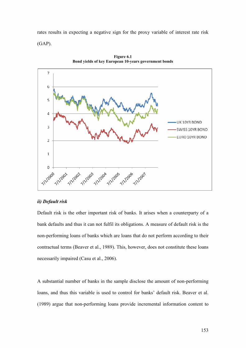
153

rates results in expecting a negative sign for the proxy variable of interest rate risk

(GAP).

Figure 6.1

Bond yields of key European 10-years government bonds

ii) Default risk

Default risk is the other important risk of banks. It arises when a counterparty of a

bank defaults and thus it can not fulfil its obligations. A measure of default risk is the

non-performing loans of banks which are loans that do not perform according to their

contractual terms (Beaver et al., 1989). This, however, does not constitute these loans

necessarily impaired (Casu et al., 2006).

A substantial number of banks in the sample disclose the amount of non-performing

loans, and thus this variable is used to control for banks’ default risk. Beaver et al.

(1989) argue that non-performing loans provide incremental information content to

154

that of loan loss allowance, and thus investors are better-off having this information

in the notes of the financial statements. They conclude that non-performing loans

capture the default risk of financial institutions and predict a negative effect on their

market values. Thus, similar to other studies (Barth et al., 1996; Venkatachalam, 1996)

the variable of non-performing loans (NPL) is also added to Equation (6.1) to control

for the default risk. Based on the discussion above a negative sign is predicted for the

NPL.

iii) Core deposit intangibles

Core deposits are an important intangible asset of banks. Demand deposits and saving

accounts even though they are payable on demand, they tend to be stable over time,

usually over many years, as deposit withdrawals are replaced by new deposits. Core

deposits constitute an intangible asset for banks because they represent customers’

loyalty. Flannery & James (1984b) provide evidence that the effective maturities of

the liabilities with a demand feature or a short notice (e.g., demand deposits, saving

accounts, and small denomination time deposits) are comparable to those of long-

term items, suggesting a core deposit behavior for these liabilities. Banks usually pay

zero or a negligible interest rate on these deposits that constitutes a cheap finance for

banks usually available to them for many years.

Ryan (2007, p. 61) argues that depositors are willing to preserve their funds in

deposits if they believe that the economy will continue to be steady and if their

desirability to invest in riskier alternative investments is low. Deposit insurance

schemes are also another important reason for depositors to continue keeping their

funds in deposits. The US was the first country to establish such a scheme through an

155

independent body the Federal Deposit Insurance Corporation (FDIC) created in 1934

after the massive bank failures of 1930-1933. The FDIC insures an amount of up to

$100,000 per depositor per insured bank which constitutes the basic insurance

amount21. EU does not have a single deposit insurance body to guarantee deposits.

Directive 94/19/EEC of European Commission requires each EU member state to

establish its own deposit insurance scheme in order to protect depositors from bank

failures. This Directive requires a minimum guarantee level of €20,000. On average,

the 27 EU member states (excluding Bulgaria and Romania) guarantee a minimum of

€27,036 as of in 200422.

Core deposits are unobservable to researchers and thus a proxy variable is needed.

Barth et al. (1996) based on the study of Flannery & James (1984b) define core

deposits as domestic deposits minus time deposits in excess of $100,000. Barth et al.

argue that foreign deposits are not insured by the FDIC and thus were excluded from

core deposits’ calculations. They also use an alternative proxy defined as domestic

deposits minus time deposits, without affecting the results.

This study proxies core deposits as deposits with no stated maturities (CORE) (e.g.,

demand deposits, current accounts, savings accounts, and generally deposits with a

demand feature). Due to data availability for European banks on account sizes

breakdown it was not possible to exclude time deposits over a specific amount, as it is

the case of Barth et al. (1996). Furthermore, the fact that EU member-states do not

have consistent deposit insurance schemes and that every member-state excludes

21 Information regarding the FDIC is retrieved via its website, Available from http://www.fdic.gov/

[Accessed 24 October 2008].

22 Data regarding minimum deposit guarantees in the EU are retrieved from the “Report on the

minimum guarantee level of Deposit Guarantee Schemes Directive 94/19/EC”. Available from http://ec.europa.eu/internal_market/bank/docs/guarantee/report_en.pdf [Accessed 24 October 2008].

156

different depositors from the deposit insurance scheme, foreign deposits are not

excluded from the calculations of core deposits. For example under the French

deposit insurance scheme foreign deposits are covered (Demirguc-Kunt et al., 2005).

The discussion above indicates a positive sign for the core deposit variable (CORE).

Non-IAS 39 variables

iv) Notional amounts of derivatives

A number of previous studies found that the notional amounts of derivatives explain

significantly market values. In particular, Riffe (1997) reports a positive relation

between the notional amounts of market-related instruments and market value of

equity, whilst Venkatachalam (1996) and Eccher et al. (1996) report a negative

relation. These opposite results can be attributed to the way investors interpret

notional amounts. In Riffe’s (1997) study, investors perceive notional amounts as an

indicator of future benefits (net expected claims of derivative contracts). In

Venkatachalam (1996) study, investors value more the risk related to the magnitude

of the involvement of banks in derivative contracts. The fact that investors do not

interpret consistently the notional amounts of derivatives, the sing of this variable

(NADER) is not predicted.

v) Credit-related off-balance sheet instruments

Banks apart from engaging in derivative contracts, they also involve in credit-related

instruments, such as commitment to extent credits, guarantees, and other contingent

liabilities. With loan commitments banks agree to lend funds to their customers and

receive a commitment fee on undrawn amounts (see Fabozzi, 2002). Other credit-

related instruments are standbys and commercial letters where banks guarantee to pay

157

the underlying amount in behalf of their costumers in case of a default. Thus, banks

expect to have a cash inflow from credit-related instruments which is the interest

earned on the contractual notional amount, and a cash outflow in case one or more of

their customers default. The sign of the coefficient of credit-related instruments will

depend on whether the present value of the expected cash inflows is greater than the

present value of the potential cash outflows (Riffe, 1997). Previous studies found that

the credit-related instruments are positively related to share prices (Riffe, 1997). The

same results are also provided by Eccher et al. (1996).

Loan Commitments and other contingent liabilities are excluded from IAS 39 but are

covered under IAS 37 “Provisions, Contingent Liabilities and Contingent Assets”

(IASB, 1998)23. Thus, banks are required to disclose in the notes the notional amounts

of these instruments24. Following Riffe (1997) and Eccher et al. (1996), the notional

amounts of credit-related off-balance sheet items are also included in the model

(OFF).

23

An exception is loan commitments that are described in para 4 of IAS 39. 24 An example on how banks disclose information of off-balance sheet items is extracted from the annual report of Fortis in 2005. The text follows is taken out of Note 50. “Credit-related financial

instruments include acceptances, commitments to extend credit, letters of credit and financial

guarantees. Fortis’s exposure to credit loss in the event of non-performance by the counterparty is

represented by the contractual notional amounts of those instruments. Fees received from these credit-

related instruments are recorded in the income statement when the service is delivered”… “The

following is a summary of the notional amounts (principal sums) of Fortis’s credit-related financial

instruments with off-balance-sheet risk at 31 December.

2005 2004

Guarantees and standby letters of credit 15,141.7 5,886.6

Commercial letters of credit 581.0 7,183.5

Documentary credits 7,048.9 4,168.1

Commitments to extend credit 156,932.7 84,628.9

Total 179,704.3 101,867.1

Of these commitments some EUR 17,617.8 million have a maturity of more than one year (2004: EUR

8,477.8 million)”.

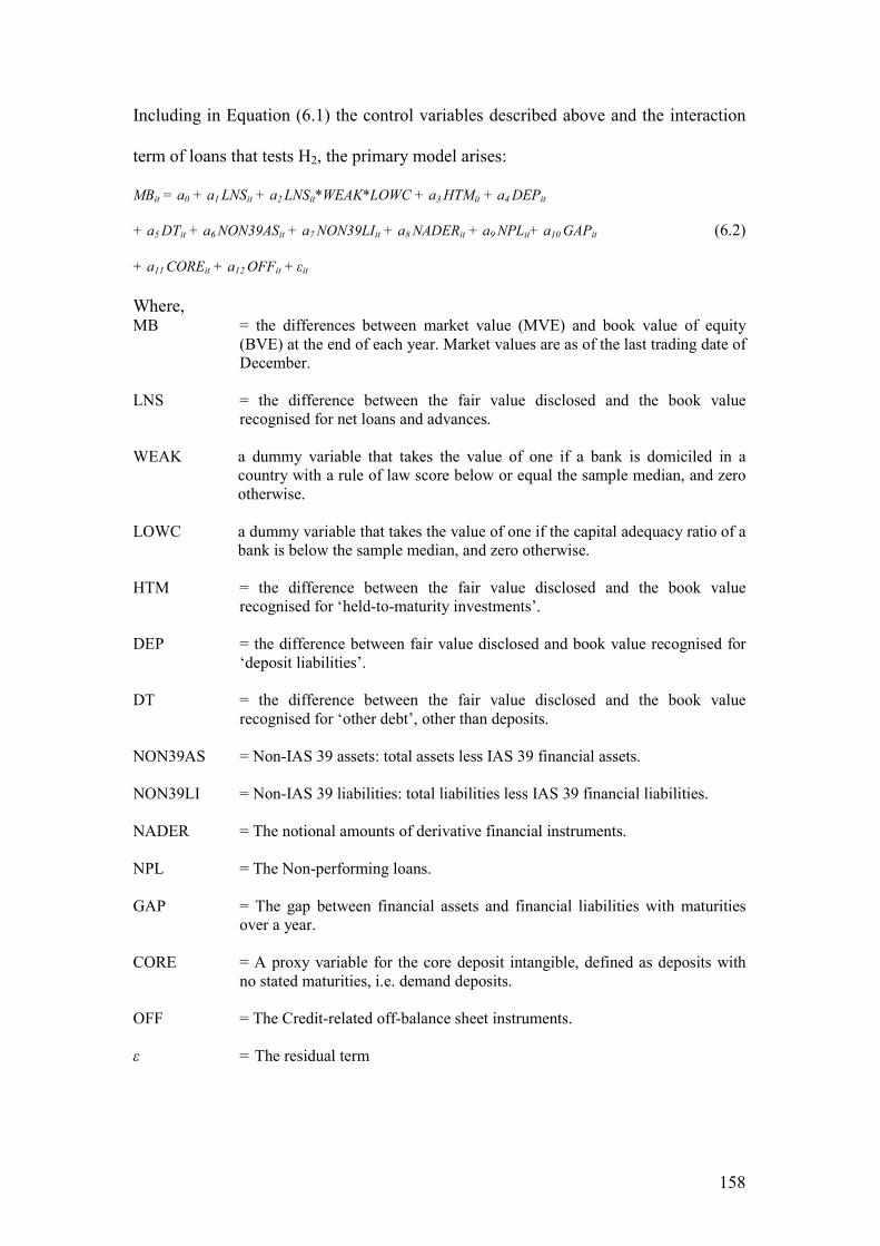
158

Including in Equation (6.1) the control variables described above and the interaction

term of loans that tests H2, the primary model arises:

MBit = a0 + a1 LNSit + a2 LNSit*WEAK*LOWC + a3 HTMit + a4 DEPit

+ a5 DTit + a6 NON39ASit + a7 NON39LIit + a8 NADERit + a9 NPLit+ a10 GAPit (6.2)

+ a11 COREit + a12 OFFit + εit Where, MB = the differences between market value (MVE) and book value of equity

(BVE) at the end of each year. Market values are as of the last trading date of December.

LNS = the difference between the fair value disclosed and the book value

recognised for net loans and advances. WEAK a dummy variable that takes the value of one if a bank is domiciled in a

country with a rule of law score below or equal the sample median, and zero otherwise.

LOWC a dummy variable that takes the value of one if the capital adequacy ratio of a

bank is below the sample median, and zero otherwise. HTM = the difference between the fair value disclosed and the book value

recognised for ‘held-to-maturity investments’. DEP = the difference between fair value disclosed and book value recognised for

‘deposit liabilities’. DT = the difference between the fair value disclosed and the book value

recognised for ‘other debt’, other than deposits. NON39AS = Non-IAS 39 assets: total assets less IAS 39 financial assets. NON39LI = Non-IAS 39 liabilities: total liabilities less IAS 39 financial liabilities. NADER = The notional amounts of derivative financial instruments. NPL = The Non-performing loans. GAP = The gap between financial assets and financial liabilities with maturities

over a year. CORE = A proxy variable for the core deposit intangible, defined as deposits with

no stated maturities, i.e. demand deposits. OFF = The Credit-related off-balance sheet instruments. ε = The residual term

159

Equation (6.2) is used to test both Hypotheses H1 and H2 and it is in undeflated form

similar to Barth et al. (1996). According to Barth & Kallapur (1996) deflating the

model by a variable (e.g., book value of equity) can increase coefficient bias and

often does not reduce heteroscedasticity.

The codification of the WEAK dummy variable is performed based on countries’ rule

of law scores provided by Kaufmann et al. (2009). According to this study the Rule

of Law measures the,

‘perceptions of the extent to which agents have confidence in and abide by the rules of society, and in particular the quality of contract enforcement, property rights, the police, and the courts, as well as the likelihood of crime and violence’.

Although the definition above does not refer explicitly to accounting rules, however,

it gives the general attitude in each country towards every rule within its jurisdiction.

Other studies in the literature used the classification provided by La Porta et al.

(1997;1998) (see Daske et al., 2008; Hail & Leuz, 2006; Lee et al., 2008; Li, 2010).

However, the classification of La Porta et al. (1997;1998) does not apply to this thesis

as it does not provide information for the rule of law of all countries in the sample.

Moreover, La Porta’s scores may be considered outdated as countries’ institutional

characteristics change over time. Table 6.1 below presents the codification of WEAK.

Countries with scores below or equal to the sample median are classified as weak

enforcements (one values) and those with scores above the sample median are

classified as strong enforcements (zero values).

160

Table 6.1

Classification of countries according to Kaufmann et al. (2009) Rule of Law Score

Country

Score 2006

WEAK variable

Classification

Score 2005

WEAK variable

Classification

Austria 1.85 0 1.81 0

Belgium 1.39 1 1.39 1

Cyprus 0.92 1 0.84 1

Czech Republic 0.75 1 0.76 1

Denmark 1.95 0 1.97 0

Finland 1.96 0 1.94 0

France 1.38 1 1.37 1

Germany 1.73 0 1.68 0

Greece 0.74 1 0.70 1

Hungary 0.80 1 0.75 1

Ireland 1.65 0 1.56 0

Italy 0.34 1 0.50 1

Lithuania 0.45 1 0.48 1

Luxemburg 1.81 0 1.90 0

Malta 1.46 0 1.39 1

Netherlands 1.72 0 1.70 0

Norway 2.00 0 1.92 0

Poland 0.28 1 0.36 1

Portugal 0.94 1 1.09 1

Slovakia 0.41 1 0.44 1

Spain 1.04 1 1.07 1

Sweden 1.88 0 1.81 0

Switzerland 1.91 0 1.93 0

UK 1.70 0 1.56 0

Mean 1.29 1.29

Median 1.43 1.39

Std Dev 0.59 0.56

The interaction term LNS*WEAK*LOWC is included in Equation (6.2) to test

whether the reliability of fair value estimates differs with respect to banks’ financial

health and countries’ ability to enforce their rules. Barth et al. (1996) find that the

market assigns a lower coefficient of fair values of loans to those banks with low

capital adequacy ratios. As the authors explain, less healthy banks may have more

incentives to overstate unrealised gains or to understate unrealised losses. However,

in a cross-country study as this one, it is likely that manager’s efficacy to manipulate

fair value estimates is a function of countries’ ability to enforce their rules. Banks

domiciled in weak enforcement rule countries have more latitude to manipulate fair

value estimates than banks domiciled in strong enforcement rule countries.

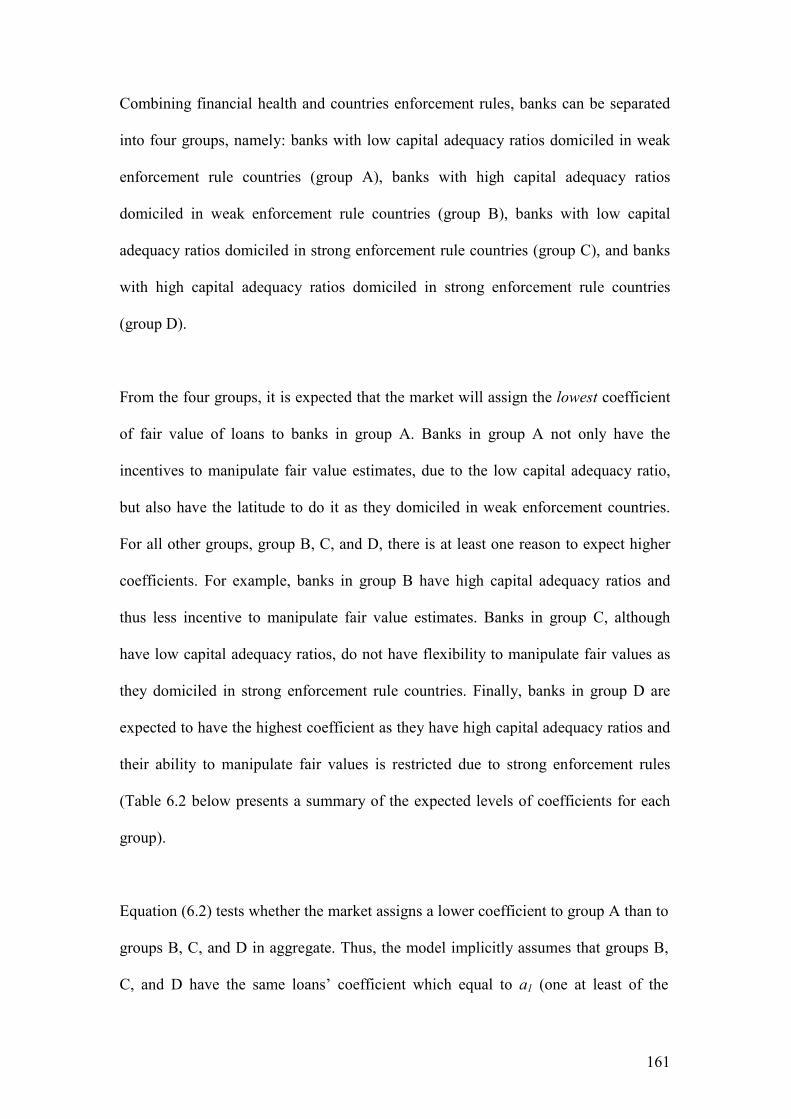
161

Combining financial health and countries enforcement rules, banks can be separated

into four groups, namely: banks with low capital adequacy ratios domiciled in weak

enforcement rule countries (group A), banks with high capital adequacy ratios

domiciled in weak enforcement rule countries (group B), banks with low capital

adequacy ratios domiciled in strong enforcement rule countries (group C), and banks

with high capital adequacy ratios domiciled in strong enforcement rule countries

(group D).

From the four groups, it is expected that the market will assign the lowest coefficient

of fair value of loans to banks in group A. Banks in group A not only have the

incentives to manipulate fair value estimates, due to the low capital adequacy ratio,

but also have the latitude to do it as they domiciled in weak enforcement countries.

For all other groups, group B, C, and D, there is at least one reason to expect higher

coefficients. For example, banks in group B have high capital adequacy ratios and

thus less incentive to manipulate fair value estimates. Banks in group C, although

have low capital adequacy ratios, do not have flexibility to manipulate fair values as

they domiciled in strong enforcement rule countries. Finally, banks in group D are

expected to have the highest coefficient as they have high capital adequacy ratios and

their ability to manipulate fair values is restricted due to strong enforcement rules

(Table 6.2 below presents a summary of the expected levels of coefficients for each

group).

Equation (6.2) tests whether the market assigns a lower coefficient to group A than to

groups B, C, and D in aggregate. Thus, the model implicitly assumes that groups B,

C, and D have the same loans’ coefficient which equal to a1 (one at least of the

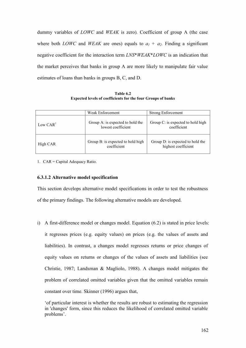
162

dummy variables of LOWC and WEAK is zero). Coefficient of group A (the case

where both LOWC and WEAK are ones) equals to a1 + a2. Finding a significant

negative coefficient for the interaction term LNS*WEAK*LOWC is an indication that

the market perceives that banks in group A are more likely to manipulate fair value

estimates of loans than banks in groups B, C, and D.

Table 6.2

Expected levels of coefficients for the four Groups of banks

Weak Enforcement Strong Enforcement

Low CAR1

Group A: is expected to hold the

lowest coefficient

Group C: is expected to hold high coefficient

High CAR

Group B: is expected to hold high

coefficient

Group D: is expected to hold the highest coefficient

1. CAR = Capital Adequacy Ratio.

6.3.1.2 Alternative model specification

This section develops alternative model specifications in order to test the robustness

of the primary findings. The following alternative models are developed.

i) A first-difference model or changes model. Equation (6.2) is stated in price levels:

it regresses prices (e.g. equity values) on prices (e.g. the values of assets and

liabilities). In contrast, a changes model regresses returns or price changes of

equity values on returns or changes of the values of assets and liabilities (see

Christie, 1987; Landsman & Magliolo, 1988). A changes model mitigates the

problem of correlated omitted variables given that the omitted variables remain

constant over time. Skinner (1996) argues that,

‘of particular interest is whether the results are robust to estimating the regression in 'changes' form, since this reduces the likelihood of correlated omitted variable problems’.

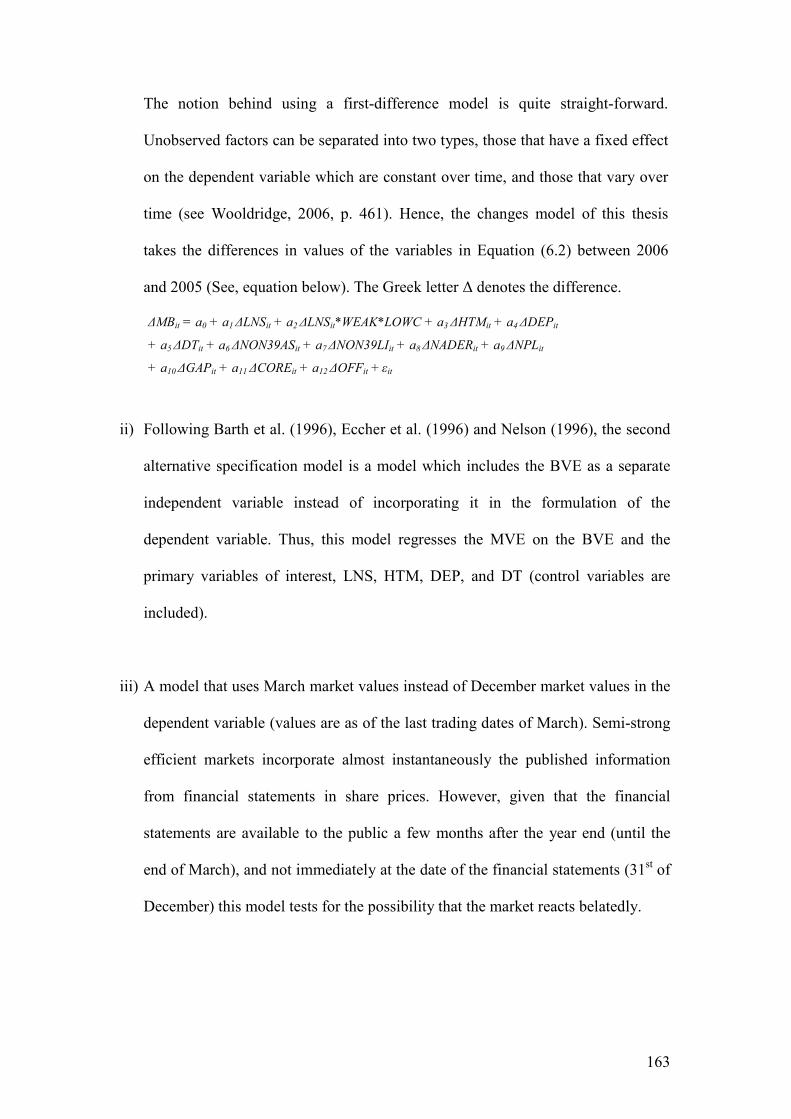
163

The notion behind using a first-difference model is quite straight-forward.

Unobserved factors can be separated into two types, those that have a fixed effect

on the dependent variable which are constant over time, and those that vary over

time (see Wooldridge, 2006, p. 461). Hence, the changes model of this thesis

takes the differences in values of the variables in Equation (6.2) between 2006

and 2005 (See, equation below). The Greek letter ∆ denotes the difference.

∆MBit = a0 + a1 ∆LNSit + a2 ∆LNSit*WEAK*LOWC + a3 ∆HTMit + a4 ∆DEPit

+ a5 ∆DTit + a6 ∆NON39ASit + a7 ∆NON39LIit + a8 ∆NADERit + a9 ∆NPLit

+ a10 ∆GAPit + a11 ∆COREit + a12 ∆OFFit + εit

ii) Following Barth et al. (1996), Eccher et al. (1996) and Nelson (1996), the second

alternative specification model is a model which includes the BVE as a separate

independent variable instead of incorporating it in the formulation of the

dependent variable. Thus, this model regresses the MVE on the BVE and the

primary variables of interest, LNS, HTM, DEP, and DT (control variables are

included).

iii) A model that uses March market values instead of December market values in the

dependent variable (values are as of the last trading dates of March). Semi-strong

efficient markets incorporate almost instantaneously the published information

from financial statements in share prices. However, given that the financial

statements are available to the public a few months after the year end (until the

end of March), and not immediately at the date of the financial statements (31st of

December) this model tests for the possibility that the market reacts belatedly.

164

iv) Similar to Barth et al. (1996) a model which includes a growth variable. This

variable is operationalised using the changes in the book values of net loans for

the last 5-years before 2005 and 2006.

v) A small number of banks, 14 in total, adopted the IFRS before they became

mandatory. These banks are likely more familiar with the standards and the fair

value measures than banks that did not have adopted the IFRS until 2005.

Furthermore, investors may value differently the early adopters assigning greater

market values. Hence, a dummy variable (EARLY) is also included in Equation

(6.2) to control for early adopters. The dummy variable EARLY takes the value

of one for those banks that have adopted the IFRS before they became mandatory

in 2005 and the value of zero otherwise.

vi) A model that controls for banks’ pension fund status. Pension plans are separated

between defined contribution schemes and defined benefit schemes. Moreover,

they separated between funded plans, where a firm establishes an independent

entity (a pension fund) with separate assets and liabilities and an independent

management (trustees), and unfunded plans where a firm operates internally the

pension plan. Defined contribution plans are by definition funded. The firm

makes regular contributions to the pension fund and bears no risk on the level of

the pensions to be paid in the future. Defined benefit plans can be either funded or

unfunded. Contrary to defined contribution plans, firm’s liability is not limited

only to regular contributions, but also extends to employees’ benefits. Thus, if the

assets of a plan cannot cover its pension liability then the firm needs to make

additional payments to the scheme. US studies support the view that the fair value

165

of pension assets and the present value of pension liability are priced by the

market and thus are reflected to share prices (Barth, 1991; Landsman, 1986).

Most European banks in this thesis operate defined benefit plans. Other banks

operate more than one type of pension scheme, such as a defined contribution

plan, a funded defined benefit plan, and an unfunded defined benefit plan. The

different types of pension plans operated by European commercial banks

precluded the use of a consistent variable for the pension obligation. Thus, similar

to other studies (Barth et al., 1996) the pension variable (PENS) is defined as the

‘fair values of plan assets less the present value of pension obligation’. For banks

that do not have a funded schemes this variable is set to be zero.

6.3.2 Recognition of derivatives’ fair values

6.3.2.1 Primary model specification

Value relevance studies on derivatives used the BSM as the primary specification

model. For example, Ahmed et al. (2006) regressed the market value of equity on the

fair values of the aggregated financial assets, the fair values of the aggregated

financial liabilities, the non-financial assets and liabilities, the fair values of

derivatives and a number of other control variables. However, due to high collinearity

in this thesis (more than 0.99) between the aggregated fair values of financial assets

and financial liabilities, the primary specification model on derivatives is based on

Ohlson (1995) model (See, Wang et al., 2005). For completeness, in an alternative

specification test results are also provided by a BSM model.

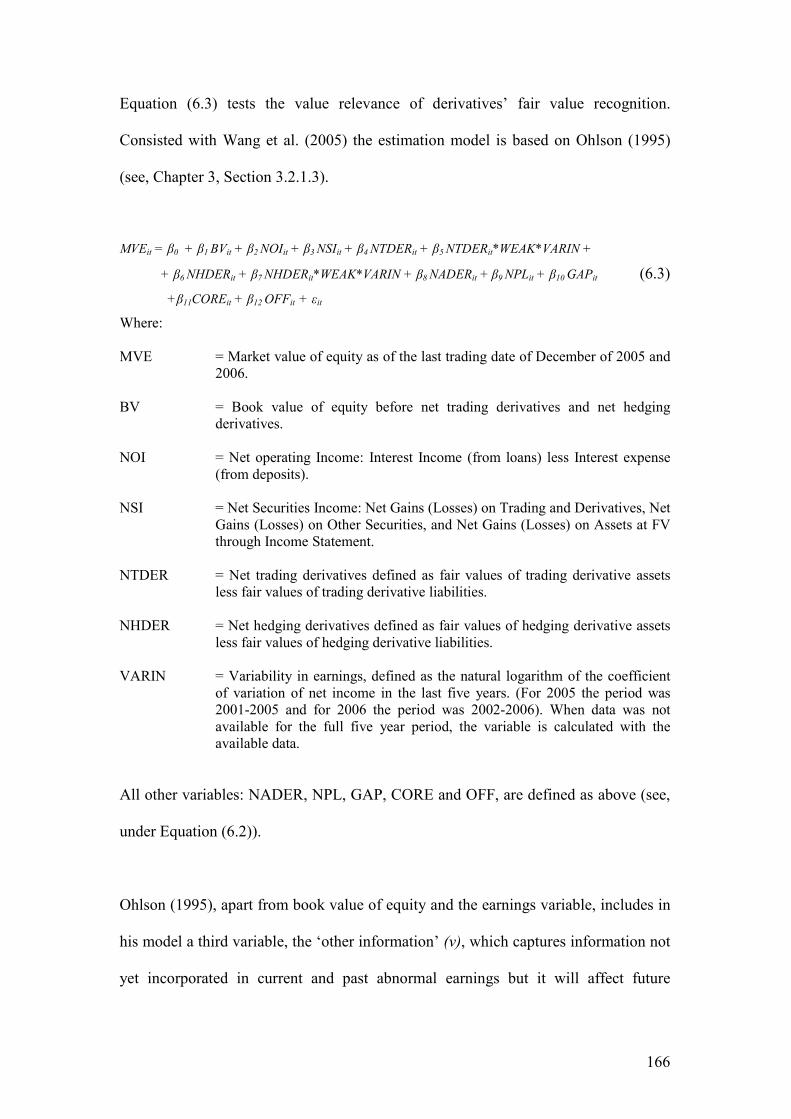
166

Equation (6.3) tests the value relevance of derivatives’ fair value recognition.

Consisted with Wang et al. (2005) the estimation model is based on Ohlson (1995)

(see, Chapter 3, Section 3.2.1.3).

MVEit = β0 + β1 BVit + β2 NOIit + β3 NSIit + β4 NTDERit + β5 NTDERit*WEAK*VARIN +

+ β6 NHDERit + β7 NHDERit*WEAK*VARIN + β8 NADERit + β9 NPLit + β10 GAPit (6.3)

+β11COREit + β12 OFFit + εit

Where: MVE = Market value of equity as of the last trading date of December of 2005 and

2006. BV = Book value of equity before net trading derivatives and net hedging

derivatives. NOI = Net operating Income: Interest Income (from loans) less Interest expense

(from deposits). NSI = Net Securities Income: Net Gains (Losses) on Trading and Derivatives, Net

Gains (Losses) on Other Securities, and Net Gains (Losses) on Assets at FV through Income Statement.

NTDER = Net trading derivatives defined as fair values of trading derivative assets

less fair values of trading derivative liabilities. NHDER = Net hedging derivatives defined as fair values of hedging derivative assets

less fair values of hedging derivative liabilities. VARIN = Variability in earnings, defined as the natural logarithm of the coefficient

of variation of net income in the last five years. (For 2005 the period was 2001-2005 and for 2006 the period was 2002-2006). When data was not available for the full five year period, the variable is calculated with the available data.

All other variables: NADER, NPL, GAP, CORE and OFF, are defined as above (see,

under Equation (6.2)).

Ohlson (1995), apart from book value of equity and the earnings variable, includes in

his model a third variable, the ‘other information’ (ν), which captures information not

yet incorporated in current and past abnormal earnings but it will affect future

167

abnormal earnings. This study assumes other information to equal zero (ν = 0). Barth

(2006b) argues that,

‘…if all assets, including intangible assets, were recognised at fair value, NI [Net Income] is simply gains and losses and ν = 0 ...because, in this setting, the persistence of abnormal earnings equals zero’.

Commercial banks recognise a substantial amount of assets and liabilities at fair value,

and thus this provides support to the operationalization of ν as equal to zero.

Coefficients β4 and β6 test hypothesis H3. Positive and significant values for these

coefficients reject H3 against the alternative hypothesis that fair values of derivatives

are value relevant (Ahmed et al., 2006).

Hypothesis H4 aims to test whether fair values of derivatives are value relevant over

and above the notional amounts of derivatives. This hypothesis is tested by examining

the significance of β4 and β6 coefficients incrementally to the coefficient of notional

amounts of derivatives, the β8.

Finally, coefficients β5 and β7 test Hypothesis H5: whether banks domiciled in weak

enforcements rule countries with higher earnings variability have lower derivatives’

coefficients than banks domiciled in strong enforcement countries with lower

earnings variability. A significant and negative coefficient for β5 and β7 supports H5.

6.3.2.2 Alternative model specification

Similar to the value relevance of fair value disclosures (Section 6.3.1.2), robustness

tests are also carried out for the value relevance of derivatives’ fair value recognition.

168

The alternative model specification includes: i) a changes model. Similar to Ahmed et

al. (2006), the model has been deflated by the beginning market value of equity, ii) a

March model, iii) a growth model, iv) an early adopters model, v) a model that

controls for banks’ pension fund status, vi) a model that disaggregates the NADER in

notional amounts of trading derivatives (NATDER) and notional amounts of hedging

derivatives (NAHDER), and vii) a model based on the BSM that regresses the market

value of equity on the aggregated fair values of financial assets and liabilities, the

non-financial assets and liabilities, the fair values of net trading and hedging

derivatives, their interaction terms and a number of control variables, as in Equation

(6.3).

6.4 Sample Selection

The objective of the study is to assess the value relevance of fair value estimates over

the first two years of the mandatory adoption of IFRS, i.e., 2005 and 2006, for the

European banking sector. Banking sector is an ideal context to examine the value

relevance of fair value accounting as the majority of banks’ assets and liabilities are

financial instruments, such as loans, investment securities, deposits, and derivatives,

all measured at fair values. The tests are performed cross-sectionally.

The concurrent adoption of the IFRS by a large number of firms across Europe

provides a unique sample to test the value relevance of fair value accounting. For the

first time in financial reporting history more than 100 countries have adopted one set

of accounting standards, the IFRS, which have substituted the national accounting

standards (at least for the listed firms).

169

The population of the study was drawn from BankScope as at 6th September 2007

and consisted of banks which met all of the following three criteria: (i) they were

classified as Commercial Banks, Cooperative Banks, Savings Banks, Bank Holding

and Holding Companies, or Real Estate and Mortgage Banks (ii) they were domiciled

in one of the 27 EU member-states, or in Switzerland or Norway; (iii) they were listed

on a stock exchange in one of the 27 EU member-states, or in Switzerland or

Norway25. 196 firms met the above criteria.

For 2005 (and 2006), 20 (21) banks were excluded due to the unavailability of their

annual report. A further 55 (53) banks were excluded due to lack of, or very poor,

information in relation to a number of variables of interest (e.g., the fair values of

financial instruments, non-performing loans). For both years a further three banks

were excluded because they did not grant loans or collect deposits. In addition, for

2005 (2006) three (one) banks were excluded because they were not listed in that year.

Finally, eight banks were excluded (for both years) because their financial year ended

on a date other than 31 December. This resulted in a sample of 107 banks for 2005

and 110 for 2006 (see, Table 6.3). The large missing values in the population result in

some countries not being represented in the final sample by any bank, such as

Bulgaria.

25

Although Norway is not an EU member, it is a member of the European Economic Area (EEA) and

as such Regulation (EC) No. 1606/2002 of the European Parliament and of the Council of 19 July 2002 applies equally to the EEA members. Thus, Norwegian listed firms, similar to the EU listed firms, were required to adopt the IFRS from 2005. Switzerland belongs neither to EU nor to EEA. However, the standard setting body in Switzerland, the Swiss Foundation for Accounting and Reporting, required all listed firms to report their accounts by 2005 either in IFRS or in US GAAP, but not in Swiss GAAP. (Available from: http:// www.iasplus.com / country / norway.htm and http:// www.iasplus.com / country / switzerl.htm [Accessed 12 January 2008]).

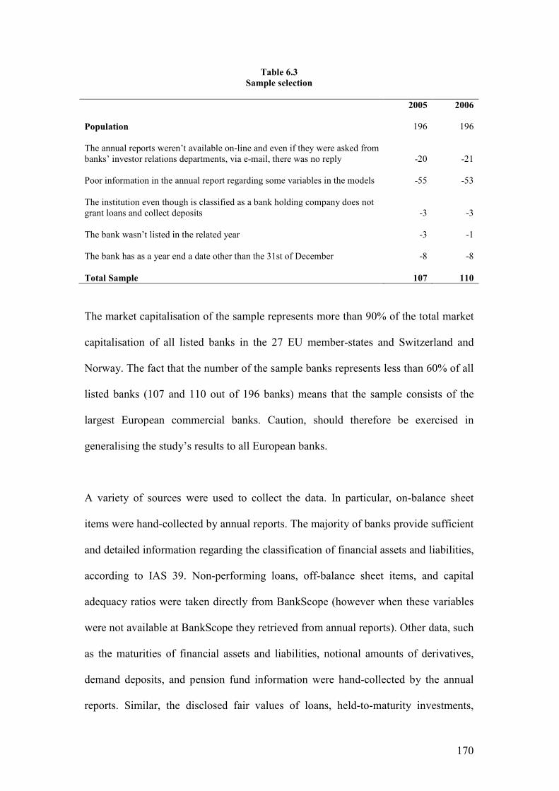
170

Table 6.3

Sample selection

2005 2006

Population

196

196

The annual reports weren’t available on-line and even if they were asked from banks’ investor relations departments, via e-mail, there was no reply

-20

-21

Poor information in the annual report regarding some variables in the models

-55 -53

The institution even though is classified as a bank holding company does not grant loans and collect deposits

-3

-3

The bank wasn’t listed in the related year

-3 -1

The bank has as a year end a date other than the 31st of December

-8 -8

Total Sample 107 110

The market capitalisation of the sample represents more than 90% of the total market

capitalisation of all listed banks in the 27 EU member-states and Switzerland and

Norway. The fact that the number of the sample banks represents less than 60% of all

listed banks (107 and 110 out of 196 banks) means that the sample consists of the

largest European commercial banks. Caution, should therefore be exercised in

generalising the study’s results to all European banks.

A variety of sources were used to collect the data. In particular, on-balance sheet

items were hand-collected by annual reports. The majority of banks provide sufficient

and detailed information regarding the classification of financial assets and liabilities,

according to IAS 39. Non-performing loans, off-balance sheet items, and capital

adequacy ratios were taken directly from BankScope (however when these variables

were not available at BankScope they retrieved from annual reports). Other data, such

as the maturities of financial assets and liabilities, notional amounts of derivatives,

demand deposits, and pension fund information were hand-collected by the annual

reports. Similar, the disclosed fair values of loans, held-to-maturity investments,

171

deposits, and other debt, were hand-collected by the annual reports. Finally,

information related to market-based data, such as share prices and number of shares

outstanding were collected from BankScope and when not available from DataStream

(for more information on data collection, see Table 6.4).

All the amounts in the sample are in million of Euros. Bank accounts that were

reported in a different currency were translated into Euros using the exchange rates

provided by the ECB on the last available date of each year. Data on exchange rates

are retrieved from DataStream (See, Appendix E, Table 2, for the exchange rates).

Table 6.4

Data Availability and Data Sources for key variables

Data description Variables Source

On-balance sheet items AFS, BHTM, FAFVPL, BLNS, NON39AS, FLFVPL, BDEP, BDT, NON39LI, BVE

Banks’ Annual Reports or BankScope

Non-performing loans NPL BankScope

Interest-sensitive assets and liabilities

ISAS, ISLI, GAP Banks’ Annual Reports

Fair values of derivatives NTDER, NHDER

Banks’ Annual Reports

Notional amounts of derivatives

NADER Banks’ Annual Reports

Fair values of on-balance sheet items

FLNS, FHTM, FDEP, FDT

Banks’ Annual Reports

Core deposit intangible proxy

CORE Banks’ Annual Reports

Capital adequacy ratios CAR

BankScope

Pension fund status PENS Banks’ Annual Reports

Off-balance sheet items OFF BankScope

Market-based data MVE, MB BankScope or DataStream

172

6.5 Conclusion

This chapter analysed the methodology to test the value relevance of fair value

disclosures and the value relevance of derivatives’ fair value recognition. The

objective is to provide further evidence on the relevance and reliability of fair value

estimates using a sample of European commercial banks that report in IFRS. The

analysis is performed cross-sectionally for the first two years of the mandatory

adoption of the IFRS, i.e., 2005 and 2006.

Previous studies provide evidence that fair value disclosures are value relevant (Barth

et al., 1996; Eccher et al., 1996; Nelson, 1996). Other studies find derivatives’ fair

value recognitions significant in explaining market values (Ahmed et al., 2006).

However, these results are based on US GAAP, such as the SFAS Nos. 107, 109, and

133. Up to now there is no evidence for the value relevance of banks’ fair value

disclosures under IFRS (e.g. IAS 32) and derivatives’ fair value recognition (e.g. IAS

39). Thus, the purpose of this thesis is to fill this gap.

The thesis also aims to shed some light on whether banks’ financial health and

earnings variability affect the reliability of fair value estimates of loans and

derivatives, respectively. Banks with low capital adequacy ratios have more

incentives to manipulate fair value estimates of loans (Barth et al., 1996). Moreover,

banks with high earnings volatility have more incentives to manipulate fair value

estimates of derivatives in order to smooth earnings (Barton, 2001). However, the

latitude of banks to manipulate fair value estimates is likely to depend on institutional

differences between the sample countries, and specifically on their efficacy to enforce

their rules. The rule of law scores, provided by Kaufmann et al. (2009) are used to

173

classify the sample countries in strong enforcement rules and weak enforcement rules.

The dummy variables of capital adequacy ratio and earnings variability were

interacted in the empirical models (see, Equations 6.2 and 6.3) with the variables of

loans and derivatives, respectively, and with a dummy variable that indicates whether

a bank is domiciled in a weak enforcement rule country or in a strong enforcement

rule country.

The empirical model of the fair value disclosures test is based on the BSM, which has

been a standard valuation model in the value relevance research (see, Landsman,

1986; Eccher et al., 1996; Venkatachalam, 1996; Ahmed et al., 2006). The model

controls for a series of variables that have been found significant in the literature in

explaining the market values of equity of banks. These variables include non-

performing loans (Beaver et al., 1989), the maturity gap between interest-sensitive

assets and liabilities, core deposits (Barth et al., 1996), notional amounts of

derivatives (Riffe, 1997), and credit-related off balance sheet instruments (Eccher et

al., 1996). Apart from the primary model specifications, results are also provided

using alternative models for robustness (e.g. changes model).

Similar to Wang et al. (2005), the empirical model of the derivatives test follows the

Ohlson (1995) model. The reason for not using again as the primary specification

model the BSM is that two of the variables in the model (i.e. BSM) were highly

correlated with each other (more than 99% correlations in both years). However, the

BSM model is run as a robustness test for completeness.

174

The next chapter develops the methodology of the second empirical part of this thesis,

the economic consequence test (i.e. cost of equity test). The findings of the value

relevance part and the economic consequence part are presented in chapters 8 and 9,

respectively.

175

Chapter 7: Research Methodology on the Cost of Equity Capital

7.1 Introduction

This chapter discusses the research methodology relating to the second main research

objective of this thesis which is to examine whether the mandatory adoption of IFRS

had an impact on the CE of European banks (see, Chapter 1, Section 1.2). As

discussed in Chapter 3 (Section 3.3), transparent accounting standards and increased

disclosure reduce information asymmetries between managers and shareholders,

reduce uncertainty, and as a consequence they lower the CE. Moreover, the adoption

of uniform accounting standards across countries reduce firms’ CE through the

reduction in adjustment costs that usually arise when comparing financial statements

prepared under different accounting standards (IASCF, 2002).

As discussed in Chapter 5, which reviewed the empirical evidence on this issue, early

studies documented the existence of an inverse relationship between increased

disclosure and the CE (Botosan, 1997; Dhaliwal et al., 1979; Diamond & Verrecchia,

1991). Studies using samples of IFRS early adopters (firms that adopted the IFRS

before they became mandatory) report mixed results (Cuijpers & Buijink, 2005;

Daske, 2006; Leuz & Verrecchia, 2000). However, empirical studies relating to the

mandatory adoption of IFRS found that this adoption led to a reduction in the CE

under some model specifications (Daske et al., 2008) and for some groups of IFRS

adopters, such as the mandatory adopters (e.g. Li, 2010).

This thesis uses empirical tests to investigate the impact of mandatory adoption of

IFRS on European commercial banks’ CE. Banks are highly affected by the adoption

of IFRS through the accounting standards IAS 32 and IAS 39 as most of their assets

176

and liabilities are financial instruments. Under these two standards, banks are

required to disclose a substantial amount of information regarding the risk of their

financial instruments. Important requirements that relate to banks’ risk are: i) either

the recognition or disclosure of fair values of all financial instruments, ii) the

recognition of previously off-balance sheet items, such as derivatives, iii) the use of

hedge accounting, and iv) relevant disclosures relating to the risk of financial

instruments (i.e. market risk, credit risk and liquidity risk) (See, Chapter 2 for more

analysis of the requirements of IAS 32 and IAS 39).

The chapter is structured as follows. Section 7.2 develops the hypotheses. Based on

the theoretical framework developed in Chapter 3 (Section 3.3), it is expected that the

adoption of IFRS will reduce banks’ CE. However, this statement needs to be tested

empirically under certain hypotheses. Section 7.3 discusses the methods used by this

thesis to estimate the CE and develops the empirical models. Four methods are used

to estimate the CE based on the theoretical models of RIVM (Gebhardt et al., 2001;

Claus & Thomas, 2001) and the EGM (Gode & Mohanram, 2003; Easton, 2004).

Section 7.4 presents the sample procedures and the data collection process. Finally,


7.2 Development of Hypotheses

Literature on the mandatory adoption IFRS provided some first results on whether the

CE has decreased after the adoption of IFRS in 2005. For example, Li (2010) found

lower CE for mandatory adopter firms. Daske et al. (2008) also reported lower CE for

firms but only when they control for the anticipation effect. In another study, Lee et al.

(2008) found greater reduction in the CE of firms domiciled in high financial

177

incentive countries (e.g. the UK) than firms domiciled in low financial incentive

countries, (e.g. Austria, Greece, and Italy). However, these studies analyze either

many industries in aggregate including banks (Daske et al., 2008) or they exclude

financial firms from the analysis because they are highly regulated and their balance

sheets are structured differently from the balance sheets of the industrial firms (Lee et

al., 2008). Thus, there is a need to examine financial institutions separately under a

homogenous sample in order to avoid the industry-effect in the model. Hence, the

sample of this thesis is a set of European commercial banks that were required to

adopt the IFRS from 2005 onward. Based on the discussion above, the first

hypothesis of the CE part is stated in its null form as follows:

H6: The mandatory adoption of IFRS did not have any material impact on banks’ CE.

As it is stated in the introduction of this Chapter, banks are mostly affected by two

IASB standards, the IAS 32 and IAS 39. Hence, this test can also be regarded with

caution as an indirect test of the relevance of these two standards in assessing banks’

risk.

Complementary to Hypothesis H6, three other hypotheses are examined to test

whether the effects on the CE vary with specific characteristics of banks. Specifically,

it is examined whether the level of analyst following, the classification of national

accounting standards, and countries’ enforcement rules have a particular effect in

determining the impact of IFRS on the CE.

Previous research has shown that the reduction in CE differs with the number of

analysts following a firm (Botosan, 1997; Richardson & Welker, 2001). Low analyst

178

following is associated with higher reduction in the CE. On the other hand, firms with

high analyst following tend to have less reduction in their CE, as analysts used to

have access to more information, before the mandatory adoption of IFRS. Hence, the

second hypothesis of the CE in its alternative form:

H7: Banks with low analyst following experienced a higher reduction in their CE than banks with high analyst following.

The study’s sample consists of banks from all EU countries and Norway and

Switzerland. Nobes (2008) classified these countries into those that fall within the

Anglo-Saxon accounting system (Cyprus, Denmark, Ireland, Malta, Netherlands,

Norway, and the UK) and the Continental accounting system (Austria, Belgium,

Czech Republic, Estonia, Finland, France, Germany, Greece, Hungary, Italy, Latvia,

Lithuania, Luxemburg, Poland, Portugal, Slovakia, Slovenia, Spain, Sweden,

Switzerland). Furthermore, Nobes (2008) argues that IFRS, as a reporting system, is

more closely related to the Anglo-Saxon one. Therefore, it is reasonable to suggest

that banks domiciled in countries which have an Anglo-Saxon accounting system are

less likely to be affected by the adoption of IFRS, because they are already using

accounting standards which are similar to the IFRS. The effects, however, on banks

domiciled in Continental countries are likely to be more pronounced because for them

IFRS represents a very different reporting system. Hence the third hypothesis of the

CE in its alternative form:

H8: Banks domiciled in ‘Continental’ countries experienced a higher reduction in their CE than banks domiciled in ‘Anglo-Saxon’ countries. The final hypothesis relates to the effect of countries’ enforcement rules on the CE.

There is evidence in the literature supporting the view that countries with strong

enforcement rules are likely to experience a higher reduction in the CE (Daske et al.,

179

2008; Li, 2010) due to significant less earnings management undertaking by the firms

in such countries (Burgstahler et al., 2006). This observations leads to the forth

hypothesis:

H9: Banks domiciled in ‘strong enforcement rule’ countries experienced a higher reduction in their CE than banks domiciled in ‘weak enforcement rule’ countries.

The next section discusses the methods used by this thesis in the estimation of the CE

(the dependent variable of the empirical models) (Section 7.3.1). It also discusses the

development of the empirical models based on which hypotheses H6 – H9 are tested

(Sections 7.3.2 and 7.3.3).

7.3 Empirical Analysis

7.3.1 Estimation of cost of equity

Following the discussion in Chapter 3 (Section 3.2.2) four methods are used to

estimate banks’ CE. Two of these methods are based on an implementation of the

RIVM as provided by Gebhardt et al. (2001) and Claus & Thomas (2001) and two are

based on the Ohlson & Juettner (2005) model as implemented by Gode & Mohanram

(2003) and Easton (2004).

7.3.1.1 The Gebhardt et al. (2001) method

The Gebhardt et al. (2001) method is an implementation of the RIVM. Due to the fact

that the RIVM involves infinite horizon periods, Gebhardt et al. (2001) made

assumptions regarding the growth of earnings in the long-term (i.e. beyond the period

of the explicit estimation of earnings). The GLS method is defined as follows:

( )TVBVE

r

rFROEBVE

r

rFROEBVEP t

GLS

GLStt

GLS

GLSttt +

+

−+

+

−+= +

++12

21

1)1( (7.1)

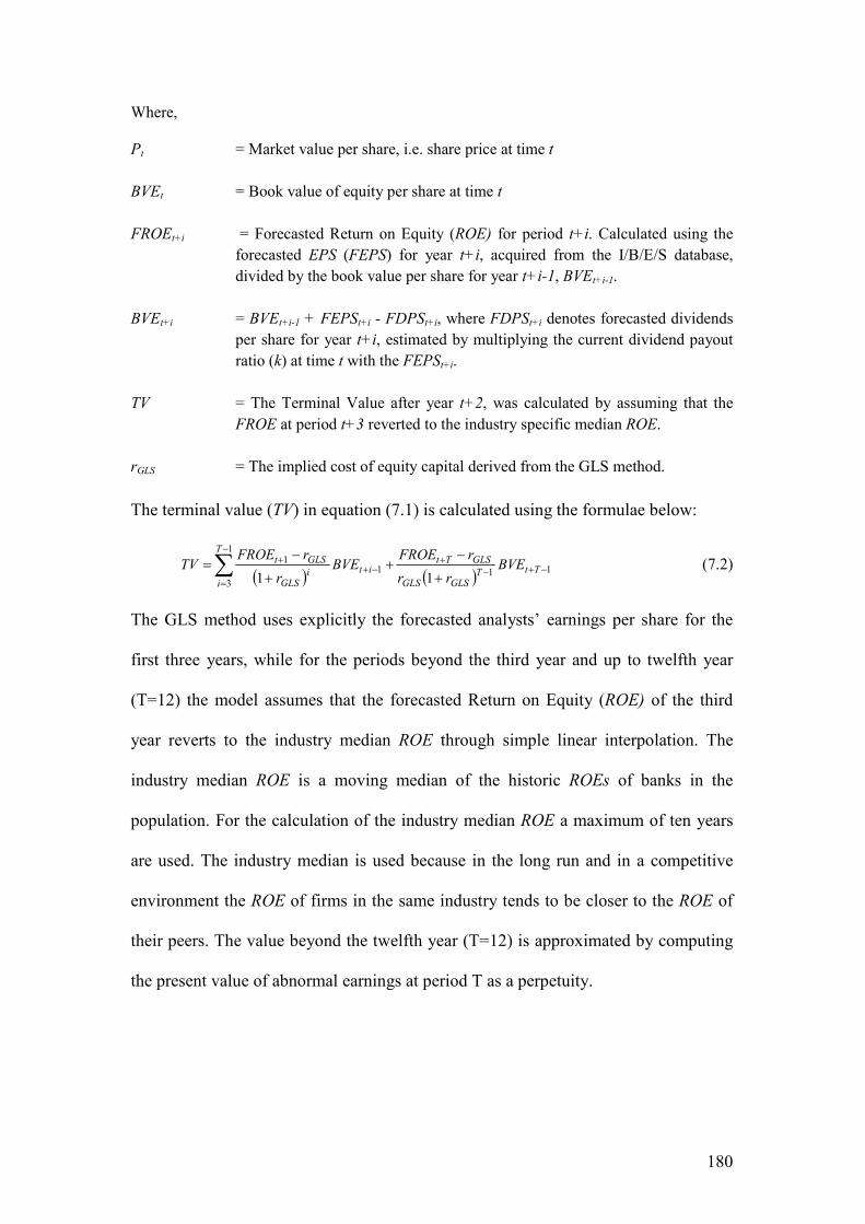
180

Where,

Pt = Market value per share, i.e. share price at time t

BVEt = Book value of equity per share at time t

FROEt+i = Forecasted Return on Equity (ROE) for period t+i. Calculated using the

forecasted EPS (FEPS) for year t+i, acquired from the I/B/E/S database,

divided by the book value per share for year t+i-1, BVEt+i-1.

BVEt+i = BVEt+i-1 + FEPSt+i - FDPSt+i, where FDPSt+i denotes forecasted dividends

per share for year t+i, estimated by multiplying the current dividend payout

ratio (k) at time t with the FEPSt+i.

TV = The Terminal Value after year t+2, was calculated by assuming that the

FROE at period t+3 reverted to the industry specific median ROE.

rGLS = The implied cost of equity capital derived from the GLS method.

The terminal value (TV) in equation (7.1) is calculated using the formulae below:

( ) ( ) 11

1

3

11

11−+−

+−

=−+

+

+

−+

+

−=∑ TtT

GLSGLS

GLSTtT

i

itiGLS

GLSt BVErr

rFROEBVE

r

rFROETV (7.2)

The GLS method uses explicitly the forecasted analysts’ earnings per share for the

first three years, while for the periods beyond the third year and up to twelfth year

(T=12) the model assumes that the forecasted Return on Equity (ROE) of the third

year reverts to the industry median ROE through simple linear interpolation. The

industry median ROE is a moving median of the historic ROEs of banks in the

population. For the calculation of the industry median ROE a maximum of ten years

are used. The industry median is used because in the long run and in a competitive

environment the ROE of firms in the same industry tends to be closer to the ROE of

their peers. The value beyond the twelfth year (T=12) is approximated by computing

the present value of abnormal earnings at period T as a perpetuity.

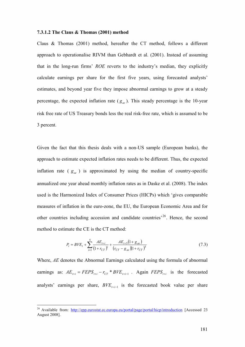
181

7.3.1.2 The Claus & Thomas (2001) method

Claus & Thomas (2001) method, hereafter the CT method, follows a different

approach to operationalise RIVM than Gebhardt et al. (2001). Instead of assuming

that in the long-run firms’ ROE reverts to the industry’s median, they explicitly

calculate earnings per share for the first five years, using forecasted analysts’

estimates, and beyond year five they impose abnormal earnings to grow at a steady

percentage, the expected inflation rate ( aeg ). This steady percentage is the 10-year

risk free rate of US Treasury bonds less the real risk-free rate, which is assumed to be

3 percent.

Given the fact that this thesis deals with a non-US sample (European banks), the

approach to estimate expected inflation rates needs to be different. Thus, the expected

inflation rate ( aeg ) is approximated by using the median of country-specific

annualized one year ahead monthly inflation rates as in Daske et al. (2008). The index

used is the Harmonized Index of Consumer Prices (HICPs) which ‘gives comparable

measures of inflation in the euro-zone, the EU, the European Economic Area and for

other countries including accession and candidate countries’26. Hence, the second

method to estimate the CE is the CT method:

( )( )

( )( )∑=

++

+−

++

++=

5

15

5

1

1

1i CTaeCT

aet

iCT

ittt

rgr

gAE

r

AEBVEP (7.3)

Where, AE denotes the Abnormal Earnings calculated using the formula of abnormal

earnings as: 1* −+++ −= itCTitit BVErFEPSAE . Again itFEPS + is the forecasted

analysts’ earnings per share, 1−+itBVE is the forecasted book value per share

26 Available from: http://epp.eurostat.ec.europa.eu/portal/page/portal/hicp/introduction [Accessed 23 August 2008].

182

calculated using the clean surplus relation as itititit FDPSFEPSBVEBVE ++−++ −+= 1 ,

and CTr is the implied CE as derived under the CT method. Similar to the GLS

method, the itFDPS + is calculated by applying the current dividend payout ratio on

the forecasted earnings per share for the period t+i ( itFEPS + ).

7.3.1.3 The Gode & Mohanram (2003) method

Apart from the RIVM, some other studies use also an Earnings Growth Model to

derive the CE (see, Daske et al., 2008; Dhaliwal et al., 2007). Gode & Mohanram

(2003) provide an empirical implementation of the Ohlson & Juettner (2005) model

which defines market value per share in terms of next-period’s expected earnings per

share; next-period’s expected dividends per share; short-term growth in earnings;

long-term perpetual growth in earnings (γ); and the CE. The model builds on the

Gordon growth model (see, Chapter 3, Section 3.2.1.1) which is based on a dividend

measure of value and the assumption of a constant dividend growth in perpetuity. The

model of Ohlson & Juettner (2005) is a parsimonious equity valuation model that

does not require the consideration of expected book values and the expected earnings

per share beyond the second year. Formula (7.4) below is the Gode & Mohanram

(2003) model which is based on Ohlson & Juettner (2005) model solved as for OJr .

( )( )120

12 −−++= γgP

FEPSAArOJ (7.4)

Where, ( )

+−=

0

112

1

P

FDPSA γ and

1

122

FEPS

FEPSFEPSg

−=

The inputs used to estimate the rOJ are the following: The forecasted analysts’

earnings per share for the following and the next year, 1FEPS and 2FEPS ,

respectively; the one year ahead forecasted dividend per share calculated as in the

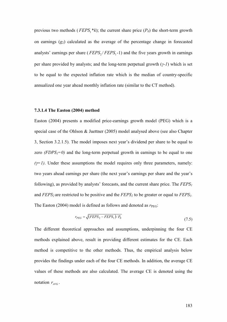
183

previous two methods ( 1FEPS *k); the current share price (P0) the short-term growth

on earnings (g2) calculated as the average of the percentage change in forecasted

analysts’ earnings per share ( 2FEPS / 1FEPS -1) and the five years growth in earnings

per share provided by analysts; and the long-term perpetual growth (γ-1) which is set

to be equal to the expected inflation rate which is the median of country-specific

annualized one year ahead monthly inflation rate (similar to the CT method).

7.3.1.4 The Easton (2004) method

Easton (2004) presents a modified price-earnings growth model (PEG) which is a

special case of the Ohlson & Juettner (2005) model analysed above (see also Chapter

3, Section 3.2.1.5). The model imposes next year’s dividend per share to be equal to

zero (FDPS1=0) and the long-term perpetual growth in earnings to be equal to one

(γ=1). Under these assumptions the model requires only three parameters, namely:

two years ahead earnings per share (the next year’s earnings per share and the year’s

following), as provided by analysts’ forecasts, and the current share price. The FEPS1

and FEPS2 are restricted to be positive and the FEPS2 to be greater or equal to FEPS1.

The Easton (2004) model is defined as follows and denoted as rPEG:

( ) 012 / PFEPSFEPSrPEG −= (7.5)

The different theoretical approaches and assumptions, underpinning the four CE

methods explained above, result in providing different estimates for the CE. Each

method is competitive to the other methods. Thus, the empirical analysis below

provides the findings under each of the four CE methods. In addition, the average CE

values of these methods are also calculated. The average CE is denoted using the

notation AVGr .

184

7.3.2 Primary analysis

The impact of the mandatory adoption of IFRS on banks’ CE is examined under a

univariate analysis, by observing the change of the CE through time, and under a

multivariate analysis using a multiple regression model similar to the one used by Lee

et al. (2008), Li (2010) and by Dhaliwal et al. (2007)27.

The period of the study covers six financial years from 2002 to 2007. Given the fact

that the official adoption of the IFRS by European firms is the year 2005, the CE

estimates in years 2002, 2003, and 2004 are regarded as the pre-IFRS period, and the

CE estimates in years 2005, 2006, and 2007 are regarded as the post-IFRS period.

The results provided under the univariate analysis should be interpreted with caution

as they do not take into account other factors, apart from the IFRS adoption, that may

have affected the CE around that time. Thus, a more complete way to test the impact

of the IFRS is to control in a regression model for other observable factors that

according to the literature are found to explain significantly the expected returns. The

primary empirical model is defined as follows:

CEit = γ0 + γ1 POSTit + γ2MANDit + γ3POST*MANDit + γ4CARit +γ5LDit + γ6BETAit + γ7VARERNit +

γ8BMit + γ9 LOG(ASSET)it + γ10 LEV + γ11RFit + γ12USLISTit+ ∑18

k

kikCOUNTRYδ + ωit (7.6)

Where,

CE = the implied cost of equity capital from the GLS method, the CT method, the OJ method, the PEG method, and the average of all the aforementioned methods (AVG).

POST = a dummy variable that takes the value of one for post-IFRS periods (on

and after 2005) and the value of zero for pre-IFRS periods (before 2005).

27 However, Dhaliwal et al. (2007) examine the expectation that the 2003 Tax Act reduced the cost of equity capital after the new tax law came into effect in May 2003.

185

MAND = a dummy variable that takes the value of one if a commercial bank did not adopt IFRS until 2005, and zero otherwise.

POST*MAND = the interaction term between POST and MAND. CAR = capital adequacy ratio. LD = net Loans to Deposits ratio. BETA = market beta, derived by regressing commercial banks’ weekly returns for

the past five years on the weekly returns of the pan-European index, DJ STOXX 600.

VARERN = variability in earnings, defined as the standard deviations in earnings over

the past five year divided the mean earnings over the same period. BM = Book to Market ratio. LOG(ASSET) = a control for banks’ size, defined as the natural logarithm of the total

assets. LEV = financial leverage, defined as the long-term debt to the book value of

equity ratio. RF = country specific risk-free rate of return. USLIST = a dummy variables that takes the value of one when a bank is listed in the

US market and zero otherwise. COUNTRY = dummy variables to control for the country-effect.

The coefficient of POST (γ1) is the coefficient of interest in examining the impact of

IFRS on the CE. A significant positive coefficient indicates that the IFRS reveal

additional risk for banks that previously (before 2005) was unknown to investors.

Risk overcomes the benefits provided by increased disclosure. On the other hand, a

negative coefficient supports the view that high quality in financial information and

increased disclosure, as it is the case with IFRS, decrease the CE. Finding the γ1

coefficient significant rejects hypothesis H6 that the mandatory adoption of IFRS did

not have any material impact on banks’ CE.

The interaction term POST*MAND tests whether there is any difference between

banks that have adopted IFRS only when they became mandatory (in 2005) and early

186

adopters, banks that voluntarily adopted IFRS prior to 2005. Coefficient γ3 aims to

capture this difference.

The remaining variables are included in equation (7.6) to control for other factors that

were found in the literature to explain significantly the variations in the CE.

Control variables

i) This study uses two industry specific control variables, the capital adequacy ratio

(CAR) and the Loans to Deposits ratio (LD). An extensive discussion of the CAR

is provided in Chapter 2, Section 2.3. According to Basel Committee, banks

should keep this ratio above the 8% in order to have adequate funds to cover

unexpected losses. Thus, whenever this ratio falls below the 8%, supervisors

demand from banks to increase capital or to liquidate some risky assets. The

higher this variable is, the lower are the regulatory costs and hence the lower the

risk for a bank28. The sign for this variable is expected to be negative (Karels et al.,

1989). The other industry specific variable, is the loans to deposit ratio (LD),

which is the control variable for banks’ liquidity and credit risk (Mansur et al.,

1993). Commercial banks use public deposits to finance their loan activity which

are regarded (the deposits) as a cheap source of finance. A high ratio of Loans to

Deposits, usually well above the unity, increases the liquidity risk of banks in the

unexpected event of significant deposit withdrawals. Moreover, high levels of

loans, as compared to deposits, increase credit risk if an important number of

banks’ clients default. Hence, based on the argument above, the sign for the

coefficient of LD is predicted to be positive.

28 Regulatory costs arise when the capital adequacy ratio of a bank falls below the minimum capital requirement which is set to be 8% for the Total Adequacy Ratio (Tier 1 and Tier 2).

187

ii) The BETA is the market beta derived by regressing banks’ weekly returns over

the past five years on the weekly returns of the pan-European index, DJ STOXX

600. Following the CAPM a positive relationship is expected between the market

beta and the CE. Market beta is widely used in the CE literature to control for

market volatility, e.g., Hail (2002), Botosan & Plumlee (2002), Daske (2006), and

Poshakwale & Courtis (2005). Other studies use other measures for market

volatility, such as last year’s return variability (Daske et al., 2008). For

completeness in a separate robustness test the return variability variable is used

instead of the market beta (see Section, 7.3.4 below).

iii) Earnings variability (VARERN) is cited in the literature as an important source of

risk in equity valuation (Beaver et al., 1970; Collins & Kothari, 1989; Easton &

Zmijewski, 1989). Thus, a variable that controls for earnings variability is

included in the empirical model. Following Gebhardt et al. (2001) the VARERN

is defined as the standard deviation of annual net earnings for the past five years

divided by the mean over the same period. In a robustness test this variable is also

operationalized with analysts’ earnings coefficient (see Section, 7.3.4).

iv) Apart from market beta, Fama and French (1993) introduced two other types of

risk, the firm size and the book-to-market ratio. Thus, the BM variable in equation

(7.6) stands for the ratio of the book value to the market value of equity. Firm size

is proxied by the LOG(ASSET) which is the natural logarithm of total assets. The

BM and the LOG(ASSET) have been used extensively as control variables in the

CE literature (see, Daske, 2006; Francis et al., 2008). Given the fact that there is

more than a single way to measure size, an alternative measure is used in a

188

robustness test, namely: the natural logarithm of the market value of equity (see

Section 7.3.4).

v) LEV denotes the financial leverage. According to Modigliani & Miller (1958),

financial leverage is inversely related to the required rate of return (i.e. the CE).

Similar to other studies (e.g. Daske et al., 2008; Lee et al., 2008; and Li, 2010),

this variable is defined as the long-term debt to the book value of equity of banks.

vi) The RF is the risk-free rate of return. Similar to Hail & Leuz (2006) and Daske et

al. (2008), Equation (7.6) controls for the time-series variation in country-specific

risk-free interest rates. RF aims to capture the differences in the level of interest

rates between countries which are a reflection of local savings rates and the

quality of institutional structures. High interest rates in a country should be related

to higher CE for the banks in this country. The RF variable is constructed using

country-specific local yields of short-term treasury bills, central bank papers, or

interbank loans.

vii) The USLIST is a dummy variable taking the value of one if a commercial bank

has securities listed in the New York Stock Exchange and zero otherwise. The

rationale for including this variable is that banks, which file registration

statements with the SEC, disclose a substantial amount of financial information.

Therefore, the disclosure requirement of IFRS would not affect them as much as

the banks which do not have a US listing.

189

viii) Finally, a set of dummy variables are included in the empirical model to control

for the country-effect.

7.3.3 Additional analysis

The empirical models in this section test hypotheses H7, H8, and H9 of the CE test.

Each of these models includes three dummy variables: the POST, the MAND, and a

dummy variable that relates to each of the hypotheses above. They also include the

interaction terms between these dummies and the same set of control variables as in

Equation (7.6). Hence, the theoretical model for H7 is as follows:

CEit = γ0 + γ1 POSTit + γ2MANDit + γ3LOWFit

+ γ4 POSTit* MANDit + γ5 POSTit* LOWFit+ γ6 MANDit* LOWFit (7.7)

+ γ7 POSTit* MANDit*LOWFit+∑9

l

litlCTRLω +∑18

k

kik COUNTRYδ + ωit

Where, LOWF is a dummy variable indicating the level of analyst following (low vs.

high analyst following). The codification of the LOWF variable in low and high

analyst following is performed by taking for each bank the average number of analyst

of the three years before the mandatory adoption of IFRS (i.e. 2002 – 2004). Based on

these estimates, the LOWF takes the value of one for banks with analyst following

below the sample’s median (low analyst following) and the value of zero otherwise

(high analyst following).

∑9

l

litlCTRLω is the set of control variables as in Equation (7.6). The interaction term

POST*LOWF in equation (7.7) tests hypothesis H7. A significant negative coefficient

190

(γ5<0) indicates that banks with low analyst following have a higher reduction in the

CE than banks with high analyst following.

Hypotheses H8 and H9 are examined under two separate empirical models. The

theoretical model for H8 is Equation (7.8):

CEit = γ0 + γ1 POSTit + γ2MANDit + γ3CONTit

+ γ4 POSTit* MANDit + γ5 POSTit* CONTit+ γ6 MANDit* CONTit (7.8)

+ γ7 POSTit* MANDit*CONTit+∑9

l

litlCTRLω +∑18

k


Where, CONT is a dummy variable taking the value of one for banks domiciled in

countries classified as Continental and the value of zero for banks domiciled in

countries classified as Anglo-Saxon (see, earlier discussion in the development of

Hypothesis H8).

The theoretical model for H9 is Equation (7.9)

CEit = γ0 + γ1 POSTit + γ2MANDit + γ3STRNGit

+ γ4 POSTit* MANDit + γ5 POSTit*STRNGit+ γ6 MANDit* STRNGit (7.9)

+ γ7 POSTit* MANDit*STRNGit+∑9

l

litlCTRLω +∑18

k


Where, STRNG is a dummy variable taking the value of one for banks domiciled in

strong enforcement rule countries and zero for banks domiciled in weak enforcement

rule countries.

Estimating equations (7.8) and (7.9) as it is, using the Eviews statistical package,

gives an error message “near singular matrix”. Agung (2009, p. 105) explains that,

‘This error message indicates that the independent variables of the model have (almost) a perfect multicollinearity based on the data sets used. However, there might

191

be nothing wrong with the model, since it could be an estimable model based on other data sets’.

Hence, given the small sample of this thesis (i.e. it involves only one industry) it is

likely that the observations are not sufficient to estimate the full theoretical models

(7.8) and (7.9). Agung (2009, p. 106) argues that the researcher, in order to solve this

problem, can use a trial-and-error method to delete some of the independent variables

that causing the problem. Thus, using the trial-and-error method, Eviews gives results

under the two empirical models below, with lower interaction terms than those

included in the theoretical models (7.8) and (7.9).

CEit = γ0 + γ1 POSTit + γ2MANDit + γ3 POSTit* CONTit

+ γ4 POSTit* MANDit*CONTit+∑9

l

litlCTRLω +∑18

k

kik COUNTRYδ + ωit (7.10)

CEit = γ0 + γ1 POSTit + γ2MANDit + γ3 POSTit* STRNGit

+ γ4 POSTit* MANDit*STRNGit+∑9

l

litlCTRLω +∑18

k

kik COUNTRYδ + ωit (7.11)

Model specifications with lower interaction terms than the full interaction terms

between the dummy variables are also used by previous studies (Daske et al., 2008;

Li, 2010). A significant negative coefficient for the interaction term POST*CONT in

equation (7.10) indicates that banks domiciled in Continental countries experienced a

greater reduction in their CE, after the mandatory adoption of IFRS, than banks

domiciled in Anglo-Saxon countries. Similarly, a significant negative coefficient for

the interaction term POST*STRNG in equation (7.11) is an evidence that banks

domiciled in strong enforcement rule countries experienced a higher reduction in their

CE than banks domiciled in weak enforcement rule countries.

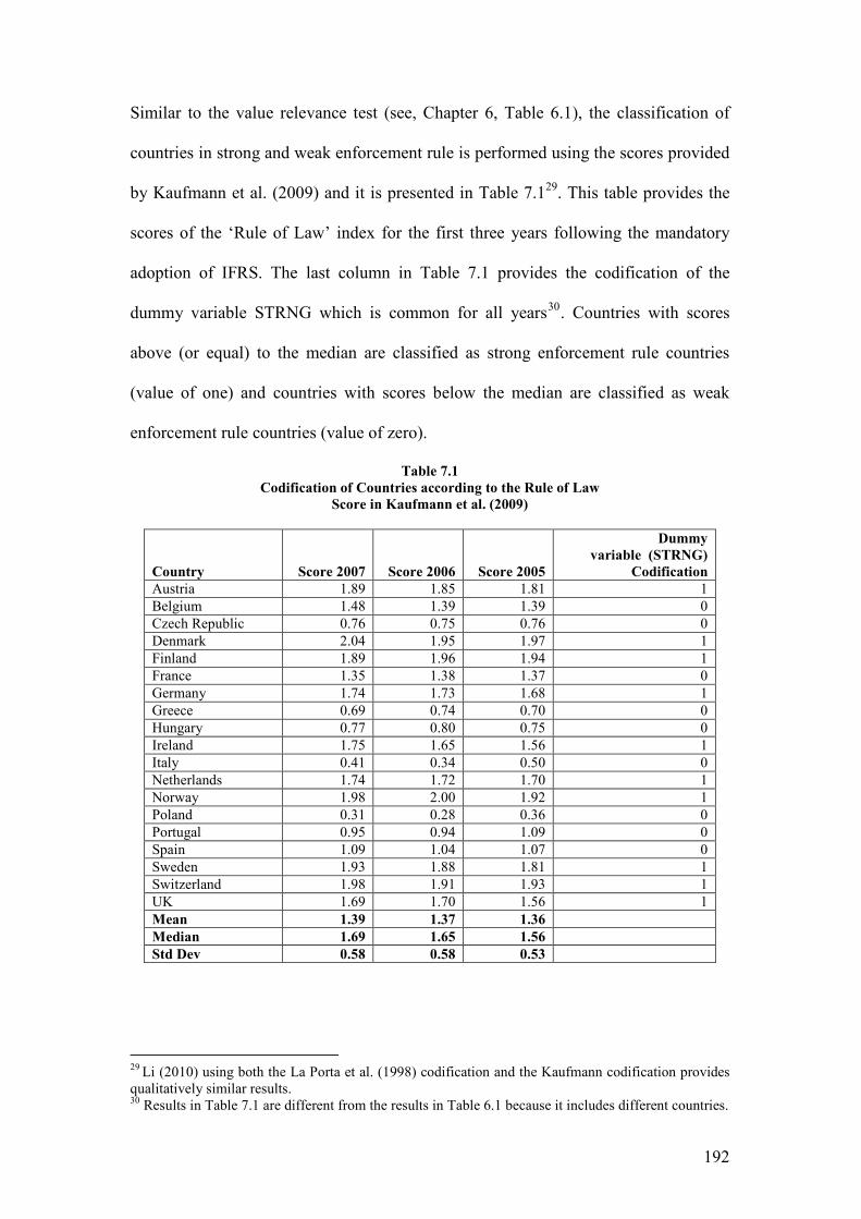
192

Similar to the value relevance test (see, Chapter 6, Table 6.1), the classification of

countries in strong and weak enforcement rule is performed using the scores provided

by Kaufmann et al. (2009) and it is presented in Table 7.129. This table provides the

scores of the ‘Rule of Law’ index for the first three years following the mandatory

adoption of IFRS. The last column in Table 7.1 provides the codification of the

dummy variable STRNG which is common for all years30. Countries with scores

above (or equal) to the median are classified as strong enforcement rule countries

(value of one) and countries with scores below the median are classified as weak

enforcement rule countries (value of zero).

Table 7.1

Codification of Countries according to the Rule of Law

Score in Kaufmann et al. (2009)

Country

Score 2007

Score 2006

Score 2005

Dummy

variable (STRNG)

Codification

Austria 1.89 1.85 1.81 1

Belgium 1.48 1.39 1.39 0

Czech Republic 0.76 0.75 0.76 0

Denmark 2.04 1.95 1.97 1

Finland 1.89 1.96 1.94 1

France 1.35 1.38 1.37 0

Germany 1.74 1.73 1.68 1

Greece 0.69 0.74 0.70 0

Hungary 0.77 0.80 0.75 0

Ireland 1.75 1.65 1.56 1

Italy 0.41 0.34 0.50 0

Netherlands 1.74 1.72 1.70 1

Norway 1.98 2.00 1.92 1

Poland 0.31 0.28 0.36 0

Portugal 0.95 0.94 1.09 0

Spain 1.09 1.04 1.07 0

Sweden 1.93 1.88 1.81 1

Switzerland 1.98 1.91 1.93 1

UK 1.69 1.70 1.56 1

Mean 1.39 1.37 1.36

Median 1.69 1.65 1.56

Std Dev 0.58 0.58 0.53

29 Li (2010) using both the La Porta et al. (1998) codification and the Kaufmann codification provides qualitatively similar results. 30 Results in Table 7.1 are different from the results in Table 6.1 because it includes different countries.

193

7.3.4 Robustness tests

A number of robustness tests are carried out in order to test the validity of the primary

findings and the findings of the additional analysis, using alternative model

specifications. Four robustness tests have been developed.

i) A number of control variables in Equation (7.6) are operationalised differently

by using different proxies. In particular, instead of using BETA, as a proxy for

market volatility, the model uses the annual return variability (RVAR) which is

defined as the standard deviation of the monthly returns at year end (see,

Gebhardt et al., 2001). VARERN is substituted by the coefficient of variation of

all the FY1 analysts’ earnings per share estimates, denoted as VARCOEF.

Finally, banks’ size is controlled by using the natural logarithm of the market

value of equity, LOG(MVE), instead of the natural logarithm of the total assets,

LOG(ASSET).

ii) A model that controls for outliers, by taking the natural logarithms of the

continuous independent variables (Wooldridge, 2006, p. 330).

iii) A model that controls for the long-term growth potential of banks (LTG). This

is proxied by the five-year consensus growth rate provided by equity analysts in

the I/B/E/S. When the growth rate is not available it is calculated from analysts’

forecasted earnings per share, using the formula (FY2/FY1-1). Gebhardt et al.

(2001) explain that analysts tend to be over-optimistic for the high long-term

growth firms which is translated to higher share prices and as a consequence to

an abnormally lower CE.

194

iv) A model that uses the risk premium for the dependent variable instead of the

implied CE (Hail & Leuz, 2006). Risk premium is calculated by subtracting

from the implied CE the risk-free rate. This model aims to test whether the

results are sensitive to other measures of the required rate of return. When the

risk premium is used as the dependent variable, the risk-free interest rate

variable (RF) is excluded from the right-hand side of the equation.

7.4 Sample procedure

The study’s population consists of European listed banks in the 27 EU member-states

and two major European economies, Switzerland and Norway. This is the same

population used in the value relevance tests, i.e., 196 European listed commercial

banks as provided by BankScope at 06/09/2007. However, due to the fact that

analysts (in I/B/E/S) do not provide estimates of the expected earnings per share (EPS)

and the growths for all banks in the population, the final sample was reduced to 88

commercial banks. For these 88 banks, data was sufficient to calculate the CE for

every year in the sample (2002 – 2007) which gives a total of 528 bank-year

observations for the CE. Excluding 108 banks from the population, some of the 29

European countries remain with zero banks and thus are not represented in the final

sample (such countries are, Bulgaria, Cyprus, Estonia, Latvia, Lithuania, Luxemburg,

Malta, Romania, Slovenia, and Slovakia).

Three major databases were used to collect the data for the calculation of the CE

(DataStream, WorldScope and I/B/E/S). Analysts’ forecasted EPS, the growth in EPS,

the actual values of EPS, and the actual values of Dividend per Share (DPS) were

taken from the I/B/E/S database. Book values per shares (BPS) and ROE ratios were

195

retrieved from WorldScope, and data on share prices from the I/B/E/S. Finally, the

information regarding country-specific inflation rates was downloaded from

Eurostat’s web site. Panel A in Table 7.2 provides a summary for the sources of the

data used to calculate the dependent variable (CE).

Table 7.2

Data Sources

Panel A:

Inputs in the CE estimates

Source

Earnings per Share forecasts I/B/E/S Earnings per Share growths I/B/E/S Actual Earnings per Share I/B/E/S Actual Dividend per Share I/B/E/S Actual Book value per Share WorldScope Return on Equity (ROE) WorldScope Share Prices (P) I/B/E/S Inflation rates EuroStat

Panel B:

Independent variables

Description

Source

ASSET Total Assets DataStream MVE Market value of Equity DataStream BETA Market beta Estimated RVAR Return Variability Estimated LD Net Loans to Total Deposits ratio Estimated BM Book to Market ratio DataStream VARERN Earnings Variability Estimated VARCOEF Coefficient of the Variation of FY1 EPS I/B/E/S CAR Capital Adequacy Ratio BankScope or

Annual Reports LTG Long-Term Growth in earnings I/B/E/S LEV Financial Leverage Estimated RF Risk-Free Rate DataStream FOLLOW Analysts’ Follow I/B/E/S

Panel B presents a summary of the sources for the independent variables. Data

relating to some of the independent variables was not directly observable and

therefore was estimated. Specifically, Market Values of Equity (MVE), Total Assets

(ASSET), Book-to-Market ratios (BM), and Risk-Free rates (RF) are retrieved from

DataStream. Capital adequacy ratios (CAR) are found on BankScope. When the CAR

was not available on BankScope the ratio was hand-collected from banks’ annual

reports or from other sources found in banks’ web sites.

196

The Loan to Deposit ratios (LD) are calculated using data from WorldScope on

Banks Net Loans and Total Deposits. Similarly, the variable of financial leverage

(LEV) is calculated using data from WorldScope dividing the Long-Term Debt with

the Book Value of Equity. The BETA, the RVAR, and the VARERN were estimated

using raw data from the DataStream, such as banks’ share price returns, returns of the

DJ STOXX 600 index, and net income data.

As with the value relevance empirical tests, all figures stated in other currencies are

converted into Euros using the exchange rates provided by the DataStream as of the

same date with the measurement date of the related variable (see, Appendix E).

7.5 Conclusion

This chapter provided the research methodology of the second empirical test of this

thesis, the economic consequence test. The chapter develops four hypotheses. The

first hypothesis tests whether the mandatory adoption of IFRS had any material

impact on banks’ CE. The other three hypotheses examine whether the decrease in the

CE is higher for specific groups of banks. These groups are banks that experience low

analyst following, domiciled in countries with Continental accounting standards, and

domiciled in Strong enforcement rule countries.

The CE is not directly observable and therefore it needs to be estimated. Similar to

Daske et al. (2008) and Li (2010), this thesis uses four methods to estimate the CE.

Two of these methods are based on an implementation of the RIVM as provided by

Gebhardt et al. (2001) and Claus & Thomas (2001) and two are based on the

197

implementation of the EGM (the Ohlson & Juettner (2005) model) as developed by

Gode & Mohanram (2003) and by Easton (2004).

The analysis involves a univariate test and a multivariate test. The univariate test

simply examines the change of the CE from 2002 to 2007. The multivariate analysis

provides a more powerful test by controlling for a number of factors that are likely to

impact on CE, i.e., the capital adequacy ratio; the ratio of loans to deposits; the

market beta; earnings variability; a size variable; the book-to-market ratio; the

financial leverage; the risk-free rate; and the US listing.

For robustness, four alternative specification models are developed: i) a model that

uses alternative variables to the variables of the primary model, ii) a model that

controls for outliers by taking the natural logarithms of the continuous independent

variables, iii) a model that controls for the growth expectations of banks by including

a long-term growth variable in the primary model, and iv) a model that uses the risk

premium as the dependent variable instead of the CE.

198

Chapter 8: Findings on the value relevance

8.1 Introduction

This chapter discusses the findings of the first empirical research, namely: the value

relevance of fair value accounting under IFRS. The findings are presented into two

separate sections. A section for the value relevance of fair value disclosures, such as

loans and advances, held-to-maturity investments, deposits, and other debt, and a

section for derivatives’ fair value recognition (net trading and hedging derivatives).

In particular, this chapter is organized as follows: Section 8.2 presents the descriptive

statistics for the dependent and the independent variables. Section 8.3 provides the

results of the regression models that test the value relevance of fair value disclosures.

The analysis begins with a discussion of the results of the primary specification

model and follows with the alternative specification models. Section 8.4 discusses the

findings on derivatives’ fair value recognition under a primary specification model

and under alternative specification models for robustness. Finally, Chapter 8.5

concludes.

8.2 Descriptive statistics

Table 8.1 reports the descriptive statistics for the variables in 2005 and 2006. On

average the market value of equity (MVE) is almost double that of its book value

(BVE). In particular, the market-to-book value ratio for 2005 is 1.73 (€13,103/7,557)

and that for 2006 is 1.84 (€15,860/8,630). Therefore, the differences between MVE

and BVE (i.e. MB), that this study attempts to explain, represent both in absolute and

relative terms, very material amounts.

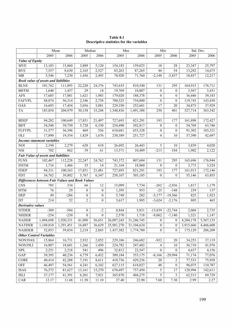
199

Table 8.1

Descriptive statistics for the variables

Mean Median Max Min Std. Dev.

2005 2006 2005 2006 2005 2006 2005 2006 2005 2006

Value of Equity

MVE 13,103 15,860 3,889 5,120 154,183 159,025 10 28 23,347 25,797

BVE 7,557 8,630 2,165 2,527 83,263 87,265 46 54 13,292 14,675

MB 5,546 7,230 1,456 2,493 70,920 71,760 -2,148 -3,837 10,857 12,217

Book value of assets and liabilities

BLNS 101,762 111,893 22,220 24,376 743,635 810,540 131 295 164,915 176,711

BHTM 1,640 1,437 29 14 19,769 18,007 0 0 3,567 3,431

AFS 17,685 17,881 1,621 1,983 179,020 188,378 0 0 36,446 39,183

FAFVPL 48,074 56,314 2,346 2,758 700,525 754,800 0 0 119,743 143,430

OAS 16,693 17,454 3,036 3,081 229,350 252,601 17 20 34,875 37,929

TA 185,854 204,979 30,158 33,248 1,348,836 1,491,388 250 401 327,714 363,542

BDEP 94,282 100,649 17,851 21,497 727,693 821,291 193 177 161,898 172,427

BDT 34,548 39,750 5,728 6,330 254,490 302,817 0 0 54,769 63,746

FLFVPL 31,577 36,396 469 536 610,681 653,328 0 0 91,302 103,321

OLI 17,890 19,554 1,829 1,676 230,389 251,727 4 10 37,390 42,697

Income statement variables

NOI 2,194 2,279 620 618 26,692 26,443 5 10 3,839 4,020

NSI 702 862 39 61 13,571 10,489 -213 -184 1,902 2,122

Fair Value of assets and liabilities

FLNS 102,467 112,228 22,247 24,762 743,372 807,604 131 295 165,696 176,944

FHTM 1,716 1,466 35 14 21,164 18,960 0 0 3,773 3,524

FDEP 94,331 100,363 17,851 21,481 727,693 821,291 193 177 161,913 172,146

FDT 34,762 39,802 5,767 6,347 258,107 303,185 0 0 55,146 63,855

Differences between Fair Values and Book Values

LNS 705 334 66 12 15,099 7,734 -262 -2,936 1,817 1,179

HTM 76 29 0 0 1,395 953 -25 -148 239 137

DEP 49 -286 0 0 5,749 282 -5,177 -19,566 825 1,923

DT 214 52 2 0 3,617 1,985 -3,624 -2,176 805 465

Derivative values

NTDER -309 -584 0 -2 8,844 5,831 -15,839 -22,744 2,068 2,735

NHDER -254 -230 0 0 2,570 1,718 -9,062 -7,140 1,521 1,147

NADER 1,494,698 1,920,331 41,090 56,651 26,097,245 31,246,745 0 0 4,284,178 5,567,135

NATDER 1,149,810 1,291,451 16,887 36,629 25,981,270 31,104,624 0 0 3,915,660 4,466,608

NAHDER 52,853 59,834 2,218 2,865 1,437,382 1,774,780 0 0 175,129 206,209

Other Control Variables

NON39AS 15,864 16,731 2,932 2,852 229,106 246,682 -932 20 34,253 37,119

NON39LI 16,807 18,601 1,266 1,450 224,782 247,482 4 10 36,710 41,976

NPL 2,251 2,218 541 496 32,812 22,547 0 0 4,637 4,156

GAP 39,395 40,236 6,779 6,432 309,184 353,175 -8,166 -29,994 71,174 77,076

CORE 40,414 42,288 7,191 8,611 418,736 429,236 20 2 77,533 75,938

OFF 46,497 54,561 4,241 6,342 627,115 618,027 48 0 96,075 110,787

ISAS 76,572 81,627 13,161 15,270 670,497 757,450 5 17 128,994 142,611

ISLI 37,177 41,391 6,201 7,921 365,870 404,275 5 3 62,513 69,729

CAR 12.17 11.68 11.50 11.10 27.40 22.90 7.60 7.30 2.99 2.27

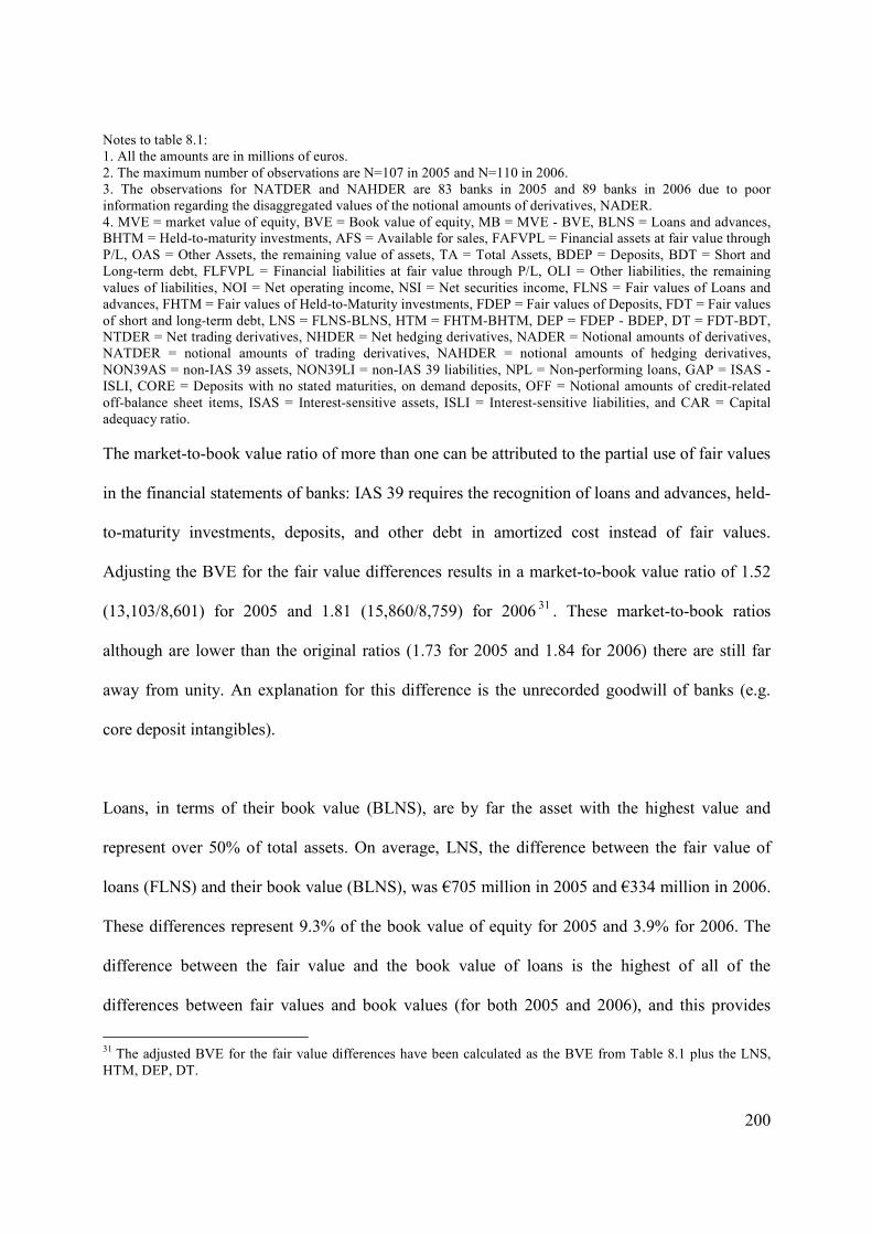
200

Notes to table 8.1: 1. All the amounts are in millions of euros.

2. The maximum number of observations are N=107 in 2005 and N=110 in 2006. 3. The observations for NATDER and NAHDER are 83 banks in 2005 and 89 banks in 2006 due to poor information regarding the disaggregated values of the notional amounts of derivatives, NADER.

4. MVE = market value of equity, BVE = Book value of equity, MB = MVE - BVE, BLNS = Loans and advances, BHTM = Held-to-maturity investments, AFS = Available for sales, FAFVPL = Financial assets at fair value through

P/L, OAS = Other Assets, the remaining value of assets, TA = Total Assets, BDEP = Deposits, BDT = Short and Long-term debt, FLFVPL = Financial liabilities at fair value through P/L, OLI = Other liabilities, the remaining

values of liabilities, NOI = Net operating income, NSI = Net securities income, FLNS = Fair values of Loans and advances, FHTM = Fair values of Held-to-Maturity investments, FDEP = Fair values of Deposits, FDT = Fair values

of short and long-term debt, LNS = FLNS-BLNS, HTM = FHTM-BHTM, DEP = FDEP - BDEP, DT = FDT-BDT, NTDER = Net trading derivatives, NHDER = Net hedging derivatives, NADER = Notional amounts of derivatives, NATDER = notional amounts of trading derivatives, NAHDER = notional amounts of hedging derivatives,

NON39AS = non-IAS 39 assets, NON39LI = non-IAS 39 liabilities, NPL = Non-performing loans, GAP = ISAS - ISLI, CORE = Deposits with no stated maturities, on demand deposits, OFF = Notional amounts of credit-related

off-balance sheet items, ISAS = Interest-sensitive assets, ISLI = Interest-sensitive liabilities, and CAR = Capital adequacy ratio.

The market-to-book value ratio of more than one can be attributed to the partial use of fair values

in the financial statements of banks: IAS 39 requires the recognition of loans and advances, held-

to-maturity investments, deposits, and other debt in amortized cost instead of fair values.

Adjusting the BVE for the fair value differences results in a market-to-book value ratio of 1.52

(13,103/8,601) for 2005 and 1.81 (15,860/8,759) for 2006 31 . These market-to-book ratios

although are lower than the original ratios (1.73 for 2005 and 1.84 for 2006) there are still far

away from unity. An explanation for this difference is the unrecorded goodwill of banks (e.g.

core deposit intangibles).

Loans, in terms of their book value (BLNS), are by far the asset with the highest value and

represent over 50% of total assets. On average, LNS, the difference between the fair value of

loans (FLNS) and their book value (BLNS), was €705 million in 2005 and €334 million in 2006.

These differences represent 9.3% of the book value of equity for 2005 and 3.9% for 2006. The

difference between the fair value and the book value of loans is the highest of all of the

differences between fair values and book values (for both 2005 and 2006), and this provides

31 The adjusted BVE for the fair value differences have been calculated as the BVE from Table 8.1 plus the LNS,

HTM, DEP, DT.

201

support for the operationalisation of the importance of capital adequacy ratio and weak

enforcement environment using, LNS*WEAK*LOWC.

Financial assets at fair value through profit or loss (FAFVPL) are the asset with the second

highest value, at 26% (27%) in 2005 (2006), followed by the available-for-sale assets (AFS), at

10% (9%). The assets with the lowest value are held-to-maturity investments. For example, for

2005 their book value (BHTM) and their fair value (FHTM) represent less than 1% of the total

assets. Moreover, the difference between their fair values and book values is, relative to that

relating to loans, small for both 2005 and 2006 (€76 million and €29 million, respectively).

With respect to the liability variables, book value of deposits (BDEP) are clearly the most

important as they represent the 53% of all liabilities (51% for 2006). However, whilst the

difference between their fair values and their book values (DEP) for 2005 is only 49 million, it is

286 million in 2006. Debt, in terms of its book value (BDT) represents only 19% (20%) of the

total liabilities. However, in contrast to DEP, the difference between the fair value and the book

value of debt (DT) is €214 million in 2005 and €52 million in 2006. The financial liabilities at

fair value through profit or loss (FLFVPL) represent the 18% (19%) of total liabilities.

Income statement variables (NOI and NSI) indicate that the majority of banks’ earnings relate to

their core business, the loan – deposit activity. For example, for 2005 the average net operating

earnings (NOI) were 2,194 million, whilst the average net securities earnings (NSI) were 702

million. Descriptive statistics regarding fair values of derivatives reveal that the net position of

trading and hedging derivatives is negative with trading derivative liabilities and hedging

derivative liabilities overcoming trading derivative assets and hedging derivative assets,

202

respectively. In particular, the net trading derivatives are -309 (-584) million in 2005 (2006) and

the net hedging derivatives are -254 (-230) million in 2005 (2006).

The descriptive statistics for control variables show that the notional amounts of derivatives

(NADER) represent very substantial amounts - an average of €1,494,698 million for 2005. The

notional amounts of derivatives are much higher than their fair values as they represent the

contractual amounts based on which the cash flows of a derivative contract are calculated. The

magnitude of notional amounts cannot be underestimated. For example, for Barclays plc in

Annual Report 2005, whilst its total assets amounted to £924.36 billion, the notional amount of

its derivatives was £17,884.44 billion. Descriptive statistics also show that, on average, the

interest sensitivity assets (ISAS) are almost double the size of interest sensitivity liabilities (ISLI)

for both years: e.g., for 2005, ISAS were €76,572 as opposed to €37,177 million for ISLI. GAP,

which represents the difference between these two variables, is the excess amount of ISAS over

ISLI. It is also noteworthy that off-balance sheet items (OFF) are relatively substantial: for both

years, they exceed the fair value of debt.

The standard deviation for all variables is large, revealing a high dispersion in the sample.

Therefore, although on average the differences between the fair value and book value of some of

the variables of interest may not be particularly large, for many banks these differences represent

very large amounts. For example, for 2005 the maximum difference between fair value and book

value for debt (DT) is €3,617 million, whilst the average difference is only €214 million. The

high dispersion in the sample may result in outliers which are a common dataset problem when

estimating the model using the Ordinary Least Squares (OLS) method. Outliers can affect the

results of the regression model because they minimize the sum of squared residuals (Wooldridge,

203

2006). Given the small population of this thesis and the fact that the sample consists of very large

banks that usually domicile in developed countries, such as the U.K., and of very small banks

that domicile in developing countries, such as Lithuania, outliers are also present in the dataset of

this thesis. Dropping some of the outliers out of the model may decrease further the sample of

the thesis and this will affect the estimated coefficients, given the smaller sample. Thus, the

regression models below were run without taking any action for outliers.

8.3 Fair value disclosures

This section provides the findings regarding the value relevance of fair value disclosures.

Evidence is provided for loans and advances, held-to-maturity investments, deposit liabilities,

and other debt. Section 8.3.1 presents the results from the primary specification model and

Section 8.3.2 discusses the results from the alternative specification models.

8.3.1 Results from the primary specification model

The correlation matrix for the regression variables indicates that some of the independent

variables are highly correlated with each other (Table 8.2, Panel A). Although it is preferable for

the correlations of the independent variables to be as low as possible, it is not clear when

multicollinearity is a problem in the dataset (Wooldridge, 2006, p. 102-103). A standard solution

is to drop one or more variables from the model: the variables that are highly correlated.

However, excluding an important variable from the model results in model misspecification and

as a consequence in bias (Greene, 2002; Wooldridge, 2006). Thus, many researchers run the

model including all variables, ignoring multiciollinearity.

2

04

Table 8.2

Correlation matrixes for the regression variables

P

anel

A:

Co

rrel

atio

ns

for

the

var

iable

s in

clu

ded

in t

he

pri

mar

y m

od

el s

pec

ific

atio

n, E

qu

atio

n (

6.2

).

M

VE

B

VE

M

B

LN

S

LN

S

*W

EA

K

*L

OW

C

HT

M

DE

P

DT

N

ON

39A

S

NO

N3

9L

I N

AD

ER

N

PL

G

AP

C

OR

E

OF

F

MV

E

1

0.9

7

0.9

5

0.2

6

0.1

1*

0.2

0

-0.0

4*

0.2

8

0.7

9

0.6

3

0.6

9

0.5

9

0.8

2

0.8

8

0.8

7

BV

E

0.9

6

1

0.8

6

0.3

1

0.1

5*

0.3

1

0.0

2*

0.3

1

0.7

6

0.7

0

0.7

3

0.6

9

0.8

5

0.9

2

0.9

1

MB

0

.95

0.8

4

1

0.1

8*

0.0

5*

0.0

5*

-0.1

3*

0.2

3

0.7

6

0.4

9

0.5

9

0.4

2

0.7

1

0.7

8

0.7

5

LN

S

0.1

7*

0.1

3*

0.2

0

1

0.8

2

0.1

7*

0.0

1*

0.0

3*

0.2

1

0.2

2

0.2

3

0.3

0

0.4

8

0.3

3

0.4

0

LN

S*W

EA

K*L

OW

C

0.1

2*

0.1

2*

0.1

1*

0.5

2

1

0.0

8*

-0.1

6*

-0.4

5

0.1

3*

0.1

5*

0.1

2*

0.1

6*

0.2

9

0.1

1*

0.3

2

HT

M

0.2

4

0.3

4

0.1

0*

-0.0

8*

-0.0

9*

1

0.0

9*

0.2

1

0.2

9

0.5

3

0.3

4

0.4

0

0.1

7*

0.2

8

0.3

4

DE

P

-0.1

4*

-0.0

9*

-0.1

9

0.0

7*

-0.0

1*

-0.0

1*

1

0.4

3

0.0

1*

0.0

4*

0.0

8*

0.1

5*

-0.0

1*

0.0

7*

-0.0

4*

DT

0

.35

0.3

5

0.3

2

-0.0

5*

-0.3

3

0.0

2*

-0.1

4*

1

0.3

0

0.3

5

0.3

0

0.3

5

0.3

3

0.4

4

0.1

5*

NO

N3

9A

S

0.7

4

0.7

1

0.7

1

0.1

2*

0.1

3*

0.3

1

-0.0

4*

0.4

4

1

0.7

3

0.8

5

0.4

6

0.6

2

0.6

9

0.6

8

NO

N3

9L

I 0

.64

0.6

8

0.5

4

0.0

7*

0.0

5*

0.5

0

-0.2

5

0.3

4

0.7

5

1

0.6

8

0.6

0

0.7

1

0.7

5

0.6

7

NA

DE

R

0.7

1

0.7

6

0.6

0

-0.0

3*

-0.0

4*

0.3

1

-0.0

1*

0.3

2

0.6

8

0.6

4

1

0.5

0

0.6

3

0.7

0

0.7

4

NP

L

0.6

6

0.7

3

0.5

1

0.2

6

0.3

9

0.3

1

-0.0

9*

0.1

0*

0.5

6

0.6

3

0.5

4

1

0.6

0

0.6

3

0.5

9

GA

P

0.7

6

0.8

2

0.6

3

0.1

5*

0.2

2

0.2

0

-0.2

6

0.2

9

0.4

7

0.6

4

0.6

4

0.7

0

1

0.8

8

0.8

4

CO

RE

0

.91

0.9

4

0.8

0

0.0

6*

0.1

2*

0.3

5

-0.2

8

0.3

1

0.6

3

0.7

6

0.7

1

0.7

1

0.8

9

1

0.8

5

OF

F

0.8

1

0.8

8

0.6

6

0.0

6*

0.0

9*

0.4

3

-0.1

4*

0.1

1*

0.5

6

0.6

6

0.7

3

0.6

2

0.7

9

0.8

7

1

1

. T

he

nu

mb

ers

at t

he

upp

er t

rian

gle

in

Pan

el A

rep

rese

nt

corr

elat

ion

s b

etw

een

th

e var

iable

s fo

r 2

005

, an

d a

t th

e lo

wer

tri

angle

co

rrel

atio

ns

bet

wee

n t

he

var

iable

s fo

r 20

06

. 2

. T

he

* i

ndic

ates

p-v

alu

es >

0.0

5.

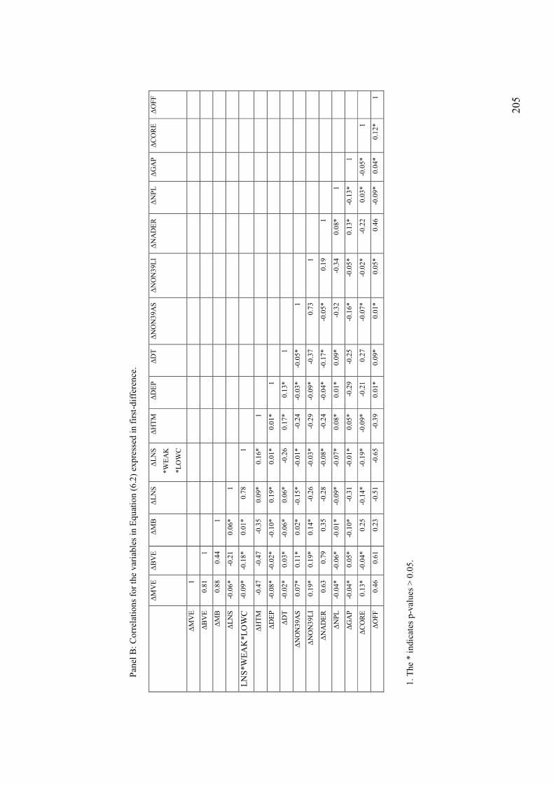
2

05

P

anel

B:

Corr

elat

ion

s fo

r th

e var

iable

s in

Eq

uat

ion (

6.2

) ex

pre

ssed

in

fir

st-d

iffe

ren

ce.

∆M

VE

∆

BV

E

∆M

B

∆L

NS

∆

LN

S

*W

EA

K

*L

OW

C

∆H

TM

∆

DE

P

∆D

T

∆N

ON

39

AS

∆

NO

N3

9L

I ∆

NA

DE

R

∆N

PL

∆

GA

P

∆C

OR

E

∆O

FF

∆M

VE

1

∆B

VE

0

.81

1

∆M

B

0.8

8

0.4

4

1

∆L

NS

-0

.06

*

-0.2

1

0.0

6*

1

LN

S*W

EA

K*L

OW

C

-0.0

9*

-0.1

8*

0.0

1*

0.7

8

1

∆H

TM

-0

.47

-0

.47

-0

.35

0

.09*

0

.16*

1

∆D

EP

-0

.08

*

-0.0

2*

-0.1

0*

0.1

9*

0

.01*

0.0

1*

1

∆D

T

-0.0

2*

0.0

3*

-0.0

6*

0.0

6*

-0

.26

0

.17

*

0.1

3*

1

∆N

ON

39

AS

0

.07*

0.1

1*

0.0

2*

-0.1

5*

-0

.01

*

-0.2

4

-0.0

3*

-0.0

5*

1

∆N

ON

39

LI

0.1

9*

0.1

9*

0.1

4*

-0.2

6

-0.0

3*

-0.2

9

-0.0

9*

-0.3

7

0.7

3

1

∆N

AD

ER

0

.63

0.7

9

0.3

5

-0.2

8

-0.0

8*

-0.2

4

-0.0

4*

-0.1

7*

-0.0

5*

0

.19

1

∆N

PL

-0

.04

*

-0.0

6*

-0.0

1*

-0.0

9*

-0

.07

*

0.0

8*

0.0

1*

0.0

9*

-0.3

2

-0.3

4

0.0

8*

1

∆G

AP

-0

.04

*

0.0

5*

-0.1

0*

-0.3

1

-0.0

1*

0.0

5*

-0.2

9

-0.2

5

-0.1

6*

-0

.05

*

0.1

3*

-0.1

3*

1

∆C

OR

E

0.1

3*

-0.0

4*

0.2

5

-0.1

4*

-0

.19

*

-0.0

9*

-0.2

1

0.2

7

-0.0

7*

-0

.02

*

-0.2

2

0.0

3*

-0.0

5*

1

∆O

FF

0

.46

0.6

1

0.2

3

-0.5

1

-0.6

5

-0.3

9

0.0

1*

0.0

9*

0.0

1*

0

.05

*

0.4

6

-0.0

9*

0.0

4*

0.1

2*

1

1.

The

* i

ndic

ates

p-v

alu

es >

0.0

5.

206

Multicollinearity is also present in previous value relevance studies (Barth et al., 1996). In this

study, researchers examine (apart from the primary specification model that suffers from high

collinearity) other model specifications, such as a first-difference specification model where the

correlations between the explanatory variables are less prevalent. Similar, to Barth et al. (1996)

the multicollinearity for the first-difference model of this study is much less of an issue (see,

Table 8.2, Panel B).

Table 8.3 reports the results of the regression analysis based on the primary specification model,

Equation (6.2). As indicated by the White (1980) chi-square test the null hypothesis of correct

model specification and the homoskedasticity assumption is not rejected for either of the two

years. White’s chi-squares are 0.0825 and 0.0656, respectively. Failing to reject the null

hypotheses of White’s test (1980) is an indication that the primary specification model, Equation

(6.2), is well specified. The model has high explanatory power: the adjusted R2 shows that in

total the independent variables explain 91% and 85% of the variation of the dependent variable

in 2005 and 2006, respectively.

The results reject the null hypothesis H1 against the alternative hypothesis that the fair values are

value relevant over and above the amortized costs. This observation holds for the disclosures of

the fair value of loans (LNS) and debt (DT). The loans variable (LNS), which represents the most

important financial asset for banks, is significant at the 0.01 level with the expected positive sign

in both years. There is also strong support for the value relevance of debt (DT) whose coefficient

is significant and negative (as hypothesized) for both years under study. The significant positive

coefficient of the loan variable (LNS) supports the findings of Barth et al. (1996) where they also

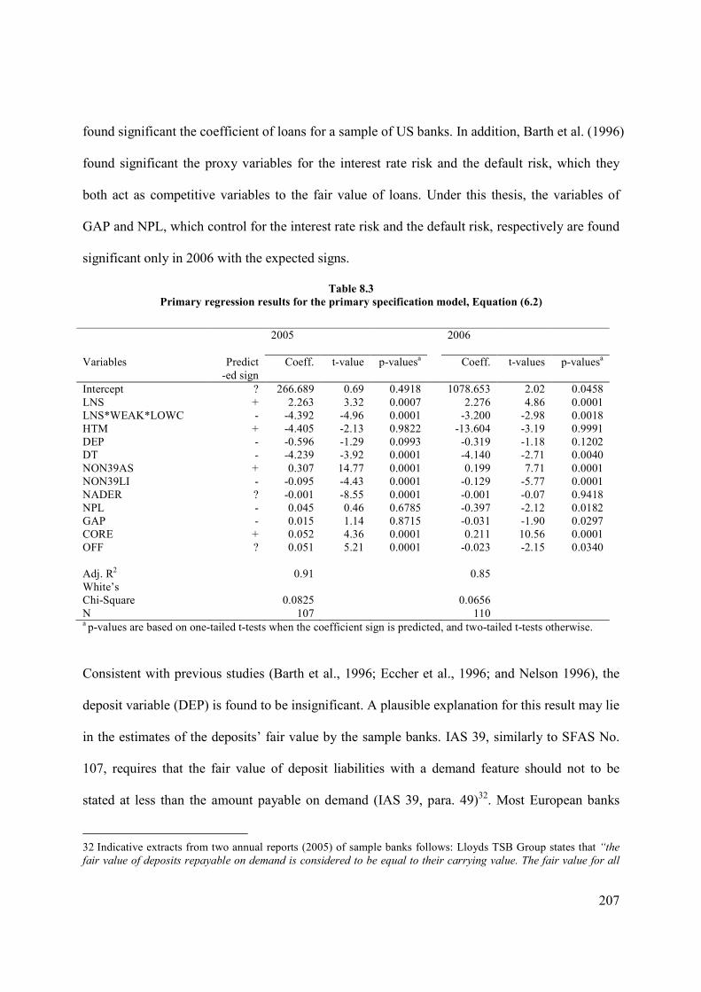
207

found significant the coefficient of loans for a sample of US banks. In addition, Barth et al. (1996)

found significant the proxy variables for the interest rate risk and the default risk, which they

both act as competitive variables to the fair value of loans. Under this thesis, the variables of

GAP and NPL, which control for the interest rate risk and the default risk, respectively are found

significant only in 2006 with the expected signs.

Table 8.3

Primary regression results for the primary specification model, Equation (6.2)

2005 2006

Variables Predict

-ed sign

Coeff. t-value p-valuesa Coeff. t-values p-valuesa

Intercept ? 266.689 0.69 0.4918 1078.653 2.02 0.0458

LNS + 2.263 3.32 0.0007 2.276 4.86 0.0001 LNS*WEAK*LOWC - -4.392 -4.96 0.0001 -3.200 -2.98 0.0018 HTM + -4.405 -2.13 0.9822 -13.604 -3.19 0.9991 DEP - -0.596 -1.29 0.0993 -0.319 -1.18 0.1202 DT - -4.239 -3.92 0.0001 -4.140 -2.71 0.0040

NON39AS + 0.307 14.77 0.0001 0.199 7.71 0.0001 NON39LI - -0.095 -4.43 0.0001 -0.129 -5.77 0.0001

NADER ? -0.001 -8.55 0.0001 -0.001 -0.07 0.9418 NPL - 0.045 0.46 0.6785 -0.397 -2.12 0.0182 GAP - 0.015 1.14 0.8715 -0.031 -1.90 0.0297 CORE + 0.052 4.36 0.0001 0.211 10.56 0.0001 OFF ? 0.051 5.21 0.0001 -0.023 -2.15 0.0340

Adj. R2 0.91 0.85 White’s Chi-Square

0.0825

0.0656

N 107 110 a p-values are based on one-tailed t-tests when the coefficient sign is predicted, and two-tailed t-tests otherwise.

Consistent with previous studies (Barth et al., 1996; Eccher et al., 1996; and Nelson 1996), the

deposit variable (DEP) is found to be insignificant. A plausible explanation for this result may lie

in the estimates of the deposits’ fair value by the sample banks. IAS 39, similarly to SFAS No.

107, requires that the fair value of deposit liabilities with a demand feature should not to be

stated at less than the amount payable on demand (IAS 39, para. 49)32. Most European banks

32 Indicative extracts from two annual reports (2005) of sample banks follows: Lloyds TSB Group states that “the

fair value of deposits repayable on demand is considered to be equal to their carrying value. The fair value for all

208

appear to state the fair value of deposits with no stated maturities at this minimum amount which

is required by the standard, i.e., their carrying amount, which may not reflect their true fair value.

Finally, held-to-maturity investments (HTM) are insignificant for both 2005 and 2006, but not in

the hypothesised direction. The negative sign of the coefficient suggests that the market

penalizes banks that classify financial assets as held-to-maturity. This may be due to the riskiness

of these investments. Held-to-maturity investments do not qualify as hedged instruments in terms

of interest rate risk (IAS 39, para. 79). Potential material variations in the value of these

investments that are not hedged, coupled with the uncertainty surrounding management’s

intention and ability to hold these instruments until maturity, may lead the market to take a

conservative stance on them, anticipating potential future losses. This is also consistent with the

view of Ryan (1999) that the long maturity and low marketability of these investments may lead

to ‘greater incompleteness, noise, and discretion’ relating to their disclosed fair values.

H2 is also strongly supported: the interaction variable (LNS*WEAK*LOWC), which permits the

fair value of loans coefficient to vary with the financial health of commercial banks and the

strength of countries’ enforcement rules, is significant for both years. The negative coefficient

for this interaction term supports the hypothesis that the market assigns a lower coefficient to the

fair value of loans of commercial banks that have a low capital adequacy ratio and domicile in

countries with weak enforcement of accounting rules (banks in group A of Table 6.2).

other deposits and customer accounts is estimated using discounted cash flows applying either market rates, where

applicable, or current rates for deposits of similar remaining maturities”. Bank Austria Creditanstalt AG states also that “To the extent that market prices were available from exchanges or other efficient markets, these were stated as

fair values. For the other financial instruments, internal valuation models were used, in particular the present value

method (discounting future cash flows on the basis of current yield curves). For fixed-rate loans and advances to, and amounts owed to, banks and customers with a remaining maturity of, or regular interest rate adjustment within

a period of, less than one year, amortised cost was stated as fair value”.

209

The findings with respect to the control variables are broadly consistent with those of past

studies. For both years the coefficients for both assets and liabilities other than those covered by

IAS 39 (NON39AS and NON39LI) are statistically different from zero at p<0.01, with the

predicted sign: positive for assets, and negative for liabilities. There is also support for the

importance of the notional amounts for derivatives (NADER), which are found significant, with

a negative sign, in 2005. This confirms the findings of past studies (e.g., Eccher et al., 1996 and

Venkatachalam, 1996), that investors associate the notional amount of derivatives with an

additional risk for banks. The results also strong support the importance of core deposits (CORE),

which are found significant in both years. This reinforces the findings of Barth et al. (1996) that

core deposits constitute an important unrecognized intangible asset which is reflected in the

market value of banks. Also, similarly to previous studies (Eccher et al., 1996 and Riffe, 1997),

the variable for credit-related off-balance sheet items (OFF) is found significant, with a positive

sign in 2005 and a negative sign in 2006. This change in sing can be attributed to a number of

factors, e.g., changes in the general financial outlook of banks might have led investors to take a

more negative stance on off-balance sheet items. Default risk, proxied by non-performing loans

(NPL), also has the predicted negative sign, supporting the view that investors interpret non-

performing loans as having a negative effect on market values (Beaver et al., 1989); but it is only

significant for 2006. Moreover, the results support the importance of interest rate risk, proxied by

GAP (i.e., the difference between financial assets and financial liabilities with maturities over a

year), which is significant for 2006. As predicted, because interest rates were in an upward trend

from the second half of 2005 and on, this variable had a negative sign, indicating that the market

had indeed taken a negative view on banks which were ‘asset sensitive’ (whose interest-sensitive

assets exceeded their interest-sensitive liabilities).

210

8.3.2 Results from the alternative specification models

This section tests the robustness of the primary findings using a number of alternative models.

Getting consistent findings under different model specifications strengthens the validity of the

primary results and increases researcher’s confidence for the relationship between the cause and

the effect, in this case the relationship between the differences in assets and liabilities’ values (i.e.

fair values less book values) and the differences in equity values (i.e. market value less book

value of equity).

i) Table 8.4 presents the results from the first-difference model that implicitly controls for

correlated omitted variables to the extent the omitted variables are constant over time.

According to White’s test the model is well specified and do not suffer from

heteroscedasticity (chi-square 0.2026). The model’s explanatory power is lower than that

of the primary model, but at 32% it is still substantial. The results with respect to the

significance of the variables of interest are substantially the same. LNS and the interaction

variable (LNS*WEAK*LOWC) are both significant at the 1% level, with the predicted

sign: positive for LNS, and negative for LNS*WEAK*LOWC. DT also continues to be

significant, with p-value of 0.0290. As in the primary model, deposits (DEP) and held-to-

maturity investments (HTM) are not significant. There are, however, some differences

concerning the significance of the control variables. CORE is still significant, as is

NADER. In contrast, GAP and NPL, which were significant for 2006 in the primary model,

are no longer significant. Finally, credit-related off-balance sheet items (OFF), and both

assets and liabilities other than those covered by IAS 39 (NON39AS and NON39LI),

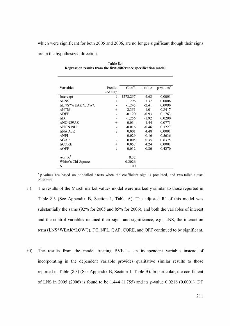
211

which were significant for both 2005 and 2006, are no longer significant though their signs

are in the hypothesized direction.

Table 8.4

Regression results from the first-difference specification model

Variables Predict -ed sign

Coeff. t-value p-valuesa

Intercept ? 1272.257 4.68 0.0001

∆LNS + 1.296 3.37 0.0006 ∆LNS*WEAK*LOWC - -1.245 -2.41 0.0090

∆HTM + -2.351 -1.01 0.8417 ∆DEP - -0.120 -0.93 0.1763

∆DT - -1.256 -1.92 0.0290 ∆NON39AS + 0.034 1.44 0.0771

∆NON39LI - -0.016 -0.46 0.3227 ∆NADER ? 0.001 4.48 0.0001 ∆NPL - 0.029 0.16 0.5636 ∆GAP - 0.005 0.35 0.6375 ∆CORE + 0.057 4.24 0.0001

∆OFF ? -0.012 -0.80 0.4270

Adj. R2 0.32 White’s Chi-Square 0.2026 N 100

a p-values are based on one-tailed t-tests when the coefficient sign is predicted, and two-tailed t-tests

otherwise.

ii) The results of the March market values model were markedly similar to those reported in

Table 8.3 (See Appendix B, Section 1, Table A). The adjusted R2 of this model was

substantially the same (92% for 2005 and 85% for 2006), and both the variables of interest

and the control variables retained their signs and significance, e.g., LNS, the interaction

term (LNS*WEAK*LOWC), DT, NPL, GAP, CORE, and OFF continued to be significant.

iii) The results from the model treating BVE as an independent variable instead of

incorporating in the dependent variable provides qualitative similar results to those

reported in Table (8.3) (See Appendix B, Section 1, Table B). In particular, the coefficient

of LNS in 2005 (2006) is found to be 1.444 (1.755) and its p-value 0.0216 (0.0001). DT

212

and the interaction term (LNS*WEAK*LOWC) are also significant with the expected

sings, e.g., for 2006, DT coefficient = -7.39 and p-value = 0.0001, and interaction term

coefficient = -2.881 and p-value = 0.0020. One difference from the primary model results

was that the deposits variable (DEP) was significant in the hypothesised direction for both

years: for 2005, coefficient of -1.036 and p-value = 0.0139; and for 2006 co-efficient of -

0.869 and p-value = 0.0010.

iv) With respect to the growth model, the growth variable (the five years change in net loans)

is found marginally significant in 2005 with a coefficient of 0.014 and a p-value of 0.0575,

and insignificant in 2006 (coefficient = 0.010, p-value = 0.2110). However, there was no

variation in the results relating to the primary variables of interest (See Appendix B,

Section 1, Table C).

v) A small number of banks (fourteen in 2005) have adopted the IFRS before the introduction

of their mandatory use in 2005. The longer experience that the market had had in dealing

with the fair value estimates of these banks could have resulted to different valuation

between the early adopters and the mandatory adopters. The dummy variable of early

adopters (EARLY) is found insignificant in both years and did not have any effect on

either the signs or the significance of the other variables (See Appendix B, Section 1, Table

D).

vi) Finally, the model that controls for banks’ pension fund status supports again the view that

the fair values of loans and the fair values of other debt are value relevant over and above

213

their amortized cost (e.g., for 2005 the coefficient of LNS is 2.192 with a p-value of 0.0010

and the coefficient of DT is -4.223 with a p-value of 0.0001). The interaction term

(LNS*WEAK*LOWC) continues to support Hypothesis H2 (coefficient = -4.298 and p-

value = 0.0001) and the results with respect to the control variables are consistent with

those reported in Table 8.3 (See Appendix B, Section 1, Table E).

Overall, the results indicate that the LNS, its interaction term (LNS*WEAK*LOWC), and the

DT are significant under all model specifications with the expected signs. Consistent to previous

studies (Barth et al., 1996), fair values of loans are found value relevant. Fair values of banks’

debt are also found significant with a negative sign. Moreover, the significant and negative

coefficient for the interaction term of loans (LNS*WEAK*LOWC) indicates that the market

assigns lower coefficient to those banks that hold low capital adequacy ratios and domicile in

countries with weak enforcement rules. As explained in the methodology chapter (Chapter 6,

Section 6.3.1.1), banks in group A have higher incentives to manipulate the fair values of loans

due to low capital adequacy ratios. Moreover, they also have the latitude to do it as they domicile

in weak enforcement rule countries.

8.4 Derivatives’ fair value recognitions

This section reports the findings regarding the value relevance of derivatives’ fair value

recognition. Section 8.4.1 presents the results from the primary specification model and Section

8.4.2 the results from the alternative specification models.

214

8.4.1 Results from the primary specification model

Correlation matrixes for the derivatives’ test indicate that the correlations between some of the

independent variables are high in the primary model (Table 8.5, Panel A). For example, the

correlation between the GAP and the NOI is 0.87 for 2005. However, the correlations are

substantial lower in the changes model (Table 8.5, Panel B). For the same variables (GAP and

NOI) the correlation fell to 0.34.

Table 8.6 reports the findings of the primary specification model, Equation (6.3). White’s chi-

square indicates that the model is well specified and does not suffer from heteroskedasticity (chi-

square = 0.0940 in 2005 and 0.0653 in 2006). Similar to previous studies (Ahmed et al., 2006)

the explanatory power of the model is high with an adjusted R-squared of 98% (97%) in 2005

(2006).

The fair values of net trading derivatives (NTDER) and net hedging derivatives (NHDER) are

found to be value relevant. Specifically, in 2005 (2006) the coefficient of NHDER is 2.804

(1.045) and its p-value is 0.0001 (0.0359). NTDER is significant in 2005 (coefficient = 2.012, p-

value = 0.0001). These findings reject the null hypothesis H3 that the fair values of derivatives

are not value relevant. Ahmed et al. (2006) provide similar results for the net fair values of

recognised derivatives.

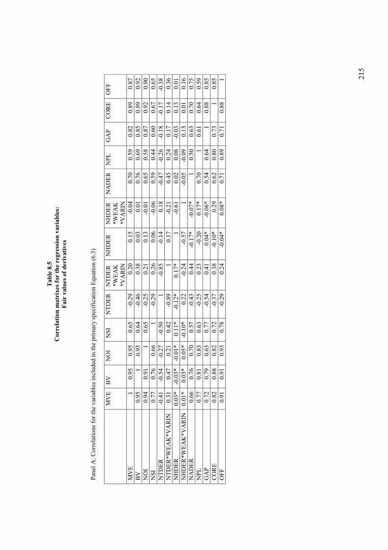
2

15

Table 8.5

Correlation matrixes for the regression variables:

Fair values of derivatives

P

anel

A:

Co

rrel

atio

ns

for

the

var

iable

s in

clu

ded

in t

he

pri

mar

y s

pec

ific

atio

n E

qu

atio

n (

6.3

)

MV

E

BV

N

OI

NS

I N

TD

ER

N

TD

ER

*W

EA

K

*V

AR

IN

NH

DE

R

NH

DE

R

*W

EA

K

*V

AR

IN

NA

DE

R

NP

L

GA

P

CO

RE

O

FF

MV

E

1

0.9

5

0.9

5

0.6

5

-0.2

9

0.2

0

0.1

5

-0.0

4

0.7

0

0.5

9

0.8

2

0.8

9

0.8

7

BV

0

.95

1

0.9

3

0.6

4

-0.4

6

0.3

8

0.0

3

0.0

1

0.7

6

0.6

9

0.8

5

0.8

9

0.9

2

NO

I 0

.94

0.9

1

1

0.6

5

-0.2

5

0.2

1

0.1

3

-0.0

1

0.6

5

0.5

8

0.8

7

0.9

2

0.9

0

NS

I 0

.77

0.7

6

0.6

6

1

-0.2

9

0.2

6

0.0

6

-0.0

6

0.5

9

0.4

4

0.6

0

0.6

7

0.6

5

NT

DE

R

-0.4

1

-0.5

4

-0.2

7

-0.5

0

1

-0.8

5

-0.1

4

0.1

8

-0.4

7

-0.2

6

-0.1

8

-0.1

7

-0.3

8

NT

DE

R*W

EA

K*V

AR

IN

0.3

1

0.4

7

0.2

1

0.4

2

-0.8

9

1

0.1

7

-0.2

1

0.4

5

0.2

4

0.1

7

0.1

4

0.3

6

NH

DE

R

0.0

3*

-0.0

3*

-0.0

1*

0.1

1*

-0.1

2*

0.1

7*

1

-0.6

1

0.0

2

0.0

8

-0.0

3

0.1

3

0.0

1

NH

DE

R*W

EA

K*

VA

RIN

0

.01

*

0.0

3*

0.0

5*

-0.1

0*

0.2

2

-0.2

4

-0.5

7

1

-0.0

5

-0.0

9

0.1

3

0.0

1

0.1

6

NA

DE

R

0.6

6

0.7

6

0.7

0

0.5

7

-0.4

3

0.4

4

-0.1

7*

-0.0

7*

1

0.5

0

0.6

3

0.7

0

0.7

5

NP

L

0.7

7

0.8

1

0.8

3

0.6

3

-0.2

5

0.2

3

-0.2

0

0.1

7*

0.7

0

1

0.6

1

0.6

4

0.5

9

GA

P

0.7

2

0.7

9

0.6

3

0.7

7

-0.5

4

0.4

1

0.0

4*

-0.0

6*

0.5

4

0.6

4

1

0.8

8

0.8

5

CO

RE

0

.82

0.8

8

0.8

2

0.7

2

-0.3

7

0.3

8

-0.1

0*

0.2

9

0.6

2

0.8

0

0.7

3

1

0.8

5

OF

F

0.9

1

0.9

1

0.9

3

0.7

8

-0.2

9

0.2

4

-0.0

4*

0.0

8*

0.7

1

0.8

9

0.7

1

0.8

8

1

2

16

Table 8.5 (continued)

Pan

el B

: C

orr

elat

ion

s fo

r th

e var

iable

s in

Eq

uat

ion (

6.3

) ex

pre

ssed

in

fir

st-d

iffe

ren

ce (

chan

ges

mo

del

).

∆

MV

E

∆B

V

∆N

OI

∆N

SI

∆N

TD

ER

∆

NT

DE

R

*W

EA

K

*V

AR

IN

∆N

HD

ER

∆

NH

DE

R

*W

EA

K

*V

AR

IN

∆N

AD

ER

∆

NP

L

∆G

AP

∆

CO

RE

∆

OF

F

∆M

VE

1

∆B

V

0.5

4

1

∆N

OI

0.1

1*

0.2

5

1

∆N

SI

0.3

6

0.0

4*

-0.1

5*

1

∆N

TD

ER

-0

.04

*

-0.3

2

-0.0

2*

0.0

2*

1

∆N

TD

ER

*W

EA

K*V

AR

IN

0.2

6

0.4

2

-0.0

3*

0.0

3*

-0.5

0

1

∆N

HD

ER

-0

.05

*

-0.2

0

-0.0

5*

-0.0

6*

-0.2

8

0.0

4*

1

∆N

HD

ER

*W

EA

K*V

AR

IN

0.0

4*

-0.0

1*

0.0

8*

0.1

2*

0.1

1*

-0.1

6*

-0.2

7

1

∆N

AD

ER

0

.28

0.5

1

0.0

1*

-0.1

2*

-0.3

9

0.6

8

0.0

4*

-0.2

1

1

∆N

PL

-0

.04

*

-0.0

1*

0.0

9*

-0.1

9*

0.0

8*

0.0

4*

-0.0

2*

0.0

3*

0.0

4*

1

∆G

AP

0

.18

*

0.2

5

0.3

4

0.1

8*

0.1

8*

-0.0

5*

-0.0

8*

0.0

7*

-0.0

6*

-0.1

8*

1

∆C

OR

E

0.1

5*

0.4

1

0.1

0*

-0.1

9*

-0.3

6

0.5

7

0.0

2*

-0.1

5*

0.5

9

0.0

4*

-0.0

5*

1

∆O

FF

0

.16

*

0.2

9

-0.0

2*

-0.0

7*

-0.1

5*

0.3

3

0.0

3*

-0.1

7*

0.5

1

0.1

7*

-0.1

2*

0.3

5

1

a. T

he

nu

mb

ers

at t

he

up

per

tri

angle

in

Pan

el A

rep

rese

nt

corr

elat

ion

s b

etw

een t

he

var

iable

s fo

r 2

00

5,

and

at

the

low

er t

rian

gle

co

rrel

atio

ns

bet

wee

n t

he

var

iable

s fo

r 20

06

. b

. T

he

* i

ndic

ates

p-v

alu

es >

0.0

5.

217

Table 8.6

Primary regression results for the primary specification model, Equation (6.3)

2005 2006


Coeff. t-value p-valuesa Coeff. t-values p-valuesa

C ? 385.342 0.88 0.3800 1050.158 1.95 0.0533 BV + 2.155 15.24 0.0001 1.614 9.85 0.0001

NOI + 0.809 1.84 0.0340 1.723 3.68 0.0002 NSI + 1.284 4.59 0.0001 2.415 5.33 0.0001

NTDER + 2.012 4.62 0.0001 0.153 0.30 0.3821 NTDER*WEAK*VARIN - -1.128 -3.66 0.0002 -1.036 -2.06 0.0209

NHDER + 2.804 7.91 0.0001 1.045 1.82 0.0359

NHDER*WEAK*VARIN - 0.373 0.99 0.8379 1.204 1.19 0.8832 NADER ? 0.000 1.41 0.1589 -0.001 -2.78 0.0064

NPL - -0.682 -5.52 0.0001 -0.782 -3.93 0.0001 GAP - 0.002 0.18 0.5728 -0.021 -1.43 0.0771

CORE + -0.073 -4.45 0.9999 0.007 0.25 0.4009 OFF ? -0.037 -2.77 0.0066 -0.047 -3.28 0.0014

Adjusted R-squared 0.98 0.97 N 107 110 White’s chi-square 0.0940 0.0653 a p-values are based on one-tailed t-tests when the coefficient sign is predicted, and two-tailed t-tests otherwise.

Null hypothesis H4 tests the statement that derivatives’ fair values are not incrementally value

relevant over and above their notional amounts. The coefficient of the notional amounts of

derivatives (NADER) is only significant in 2006 with a negative sign. This finding is consistent

with previous studies (Venkatachalam, 1996) and the results presented in Table 8.3 of this thesis

(the value relevance disclosures). The concurrent significance of the NADER with the NTDER

and NHDER in 2006 indicates that the fair values of derivatives are value relevant over and

above their notional amounts. This leads to a rejection of the null hypothesis, H4. Investors

regard fair values of derivatives, which represent the current values of derivative contracts, as

providing additional information content to their notional (contractual) amounts. Fair values

show whether derivative contracts are a value-added activity for banks (positive fair values of

derivatives) or whether they decrease banks’ market value of equity (negative fair values). In

218

contrast, the notional amounts of derivatives only provide the magnitude of the involvement of a

bank in derivative contracts without revealing whether the bank is better-off from this activity.

The interaction term of trading derivatives (NTDER*WEAK*VARIN) is found negative and

significant in both years, e.g., for 2005 the coefficient = -1.128 and the p-value = 0.0002. This

result supports Hypothesis H5 that the market assigns a lower coefficient to the fair values of

derivatives of banks with high earnings volatility, domiciled in weak enforcement rule countries.

This finding is consistent with Barton (2001) that reports evidence that firms use derivatives to

smooth earnings. Thus, investors are more concern with the fair value estimates of derivatives of

banks that experience high earnings volatility. However, this result does not hold for hedging

derivatives (e.g. for 2005 the p-value of the interaction term NHDER*WEAK*VARIN is

0.8379).

As predicted the book value of equity before trading and hedging derivatives (BV), the net

operating income (NOI), and the net securities income (NSI) are all significant for both years

with positive signs. These findings are consistent with those of Wang et al. (2005) who also

found the book value of equity and the earnings variables significant with positive coefficients.

Regarding the other control variables only non-performing loans (NPL) and off-balance sheet

items (OFF) are found value relevant in both years. NPL also holds the expected negative

coefficient. NADER is only found significant in 2006 with a negative sign. Contrary to the

results from the value relevance disclosure test (see, Table 8.3) the CORE variable is

insignificant.

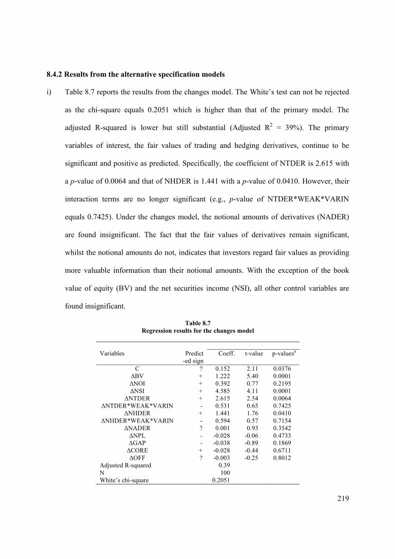
219

8.4.2 Results from the alternative specification models

i) Table 8.7 reports the results from the changes model. The White’s test can not be rejected

as the chi-square equals 0.2051 which is higher than that of the primary model. The

adjusted R-squared is lower but still substantial (Adjusted R2 = 39%). The primary

variables of interest, the fair values of trading and hedging derivatives, continue to be

significant and positive as predicted. Specifically, the coefficient of NTDER is 2.615 with

a p-value of 0.0064 and that of NHDER is 1.441 with a p-value of 0.0410. However, their

interaction terms are no longer significant (e.g., p-value of NTDER*WEAK*VARIN

equals 0.7425). Under the changes model, the notional amounts of derivatives (NADER)

are found insignificant. The fact that the fair values of derivatives remain significant,

whilst the notional amounts do not, indicates that investors regard fair values as providing

more valuable information than their notional amounts. With the exception of the book

value of equity (BV) and the net securities income (NSI), all other control variables are

found insignificant.

Table 8.7

Regression results for the changes model


Coeff. t-value p-valuesa

C ? 0.152 2.11 0.0376 ∆BV + 1.222 5.40 0.0001

∆NOI + 0.392 0.77 0.2195 ∆NSI + 4.585 4.11 0.0001

∆NTDER + 2.615 2.54 0.0064 ∆NTDER*WEAK*VARIN - 0.531 0.65 0.7425

∆NHDER + 1.441 1.76 0.0410

∆NHDER*WEAK*VARIN - 0.594 0.57 0.7154 ∆NADER ? 0.001 0.93 0.3542

∆NPL - -0.028 -0.06 0.4733 ∆GAP - -0.038 -0.89 0.1869

∆CORE + -0.028 -0.44 0.6711 ∆OFF ? -0.003 -0.25 0.8012

Adjusted R-squared 0.39

N 100 White’s chi-square 0.2051

220

ii) The results of the March model show that the fair values of trading (NTDER) and hedging

(NHDER) derivatives are only significant in 2005 (See, Appendix B, Section 2, Table A).

The interaction term of trading derivatives (NTDER*WEAK*VARIN) is significant and

negative in both years supporting again the view that the market assigns a lower coefficient

to the fair values of trading derivatives of banks with high earnings volatility, domiciled in

weak enforcement rule countries. NADER is found concurrently significant with the fair

values of derivatives. This rejects hypothesis H4, which means that fair values of

derivatives are value relevant incrementally to their notional amounts. Consistent with the

results of the primary model (Table 8.6) the variables of BV, NOI, NSI, NPL, and OFF are

significant.

iii) The results of the model which incorporates the growth variable (LNS_5YR_CH) show

that this variable is found to be positive but insignificant in both years (e,g., for 2005

coefficient = 0.004, p-value = 3440). The inclusion of this variable in the primary model do

not changes the results with respect to the other variables (See, Appendix B, Section 2,

Table B).

iv) The early adopters’ dummy variable is also found insignificant under the derivatives’

model (See, Appendix B, Section 2, Table C). For 2005 its coefficient is 1,084.55 and p-

value = 0.3450 and for 2006 coefficient = 945.72 and p-value = 0.5286. Fair values of

hedging derivatives (NHDER) continue to be significant in both years and fair values of

trading derivatives (NTDER) are only significant in 2005 (coefficient = 2.014 and p-value

= 0.0001). Consistent with the findings of the primary model (Table 8.6) only the

interaction term of trading derivatives is found significant, supporting again Hypothesis H5.

221

NADER is concurrently significant with the fair values of derivatives in 2006, whilst the

NPL and the OFF are found significant with a negative coefficient in both years.

v) The model that controls for the pension fund status of banks (PENS) indicates that

investors do not regard the pension fund deficit or surplus of banks as an equity related

figure (See Appendix B, Section 2, Table D). For example, the coefficient of PENS in

2005 is positive and amounts to 0.558 with a p-value = 0.1926. The findings with respect

to the other variables are similar to that of the primary model specification.

vi) A model that disaggregates the notional amounts of derivatives (NADER) into notional

amounts of trading (NATDER) and notional amounts of hedging derivatives (NAHDER)

has also been tested (See Appendix B, Section 2, Table E)33. Similar to Venkatachalam

(1996), this model supports the view that investors are better-off having available the

disaggregated information for the notional amounts of derivatives. The adjusted R-squared

has increased from 97% to more than 99%. Another important finding is that the White’s

chi-square is also found to be extremely high, 0.99 in 2005 and 0.98 in 2006. The fair value

of trading derivatives (NTDER) and hedging derivatives (NHDER) are found value

relevant in both years (e.g., for 2006 the coefficient of NTDER equals 1.725 and the p-

value = 0.0001, and the coefficient of NHDER equals 1.507 and the p-value = 0.0027). The

interaction term of trading derivatives (NTDER*WEAK*VARIN) for 2005 is significant

and negative as in the previous model, whilst the interaction term of hedging derivatives

(NHDER*WEAK*VARIN) is found insignificant in both years. With respect to the

33 This model results in a substantial smaller sample (for 2005, N = 83, and for 2006, N = 88) due to lack of the disaggregated information regarding the notional amounts of total derivatives (NADER) in trading and hedging

notional amounts.

222

disaggregated values of trading (NATDER) and hedging (NAHDER) derivatives, only the

notional amounts of trading derivatives have a significant negative relationship to the

market value of equity (p-value = 0.0078 in 2005, and p-value = 0.0001 in 2006). These

results provide additional support to the findings of the previous models which show that

the fair values of derivatives are incrementally value relevant over and above their notional

amounts. Consistent with the results of the previous models the coefficient of NPL is

negative and significant in both years. OFF is found insignificant, whilst core deposits

(CORE) are value relevant only in 2006 with the expected sign (coefficient = 0.051 and p-

value = 0.0083). Finally, as expected, the book value of equity before derivatives’ fair

values (BV) is significantly related to the market value of equity. Regarding the earnings

variables, only the net securities income (NSI) is found significant and positive in 2005,

whilst the net operating income (NOI) is no longer value relevant.

vii) Venkatachalam (1996) and Ahmed et al. (2006) used the BSM to provide results for

derivatives’ fair values. As discussed in Chapter 6 (Section 6.3.2.1), due to the fact that

two variables in the BSM, the aggregated fair values of financial assets (FVFAS) and the

aggregated fair values of financial liabilities (FVFLI) were highly correlated (more than

99% correlation in both years), a decision was taken not to use the BSM as the primary

specification model. Instead, a model based on Ohlson (1995) model served as the study’s

primary model. However, for completeness a model based on the BSM is also tested (See,

Appendix B, Section 2, Table F). Fair values of hedging derivatives (NHDER) continue to

be significant in both years (for 2005 coefficient = 2.277 and p-value = 0.0001 and for

2006 coefficient = 2.897 and p-value = 0.0001). In contrast, fair values of trading

223

derivatives (NTDER) are no longer significant. For both years, the coefficient of the

notional amounts of derivatives (NADER) has a negative sign and it is significant. The

other control variables have the expected signs. The non-performing loans (NPL) continue

to be significant with a negative sing in both years. The maturity gap (GAP) is value

relevant in 2006 with a coefficient of -0.038 and a p-value of 0.0019. Similar to previous

studies (Barth et al., 1996), the core deposits (CORE) have a positive impact on market

values. Finally, the aggregated fair values (FVFAS) of financial assets and financial

liabilities (FVFLI) had the predicted signs, positive for assets and negative for liabilities.

The same observation also holds for non-IAS 39 assets and liabilities.

Overall, the derivatives’ tests indicate that the recognised fair values of trading and hedging

derivatives are value relevant, which means that investors incorporate the new information

provided by the fair values in their investment decisions. In addition, fair values of derivatives

have incremental explanatory power over and above their notional amounts. Results also support

the view that investors assign a lower coefficient to the fair values of trading derivatives for

those banks with high earnings volatility that domiciled in weak enforcement rule countries. This

finding provides support to the results of Barton (2001) that firms use derivatives to smooth

earnings. However, this last result does not hold for hedging derivatives.

8.4.3 The use of hedging derivatives by European banks

As shown in the previous section, European banks do not use hedging derivatives to smooth

earnings. In order to investigate further the role of hedging derivatives, this study examines

whether banks use hedging derivatives solely for their primary purpose, which is to hedge their

224

positions. Carter & Sinkey (1998) provide evidence that interest-rate derivatives of a sample of

US banks are positively related to the maturity gap of financial assets and liabilities. This finding

indicates that US banks use derivatives to reduce the interest rate risk related to the maturity gap

of net financial assets. Hence, this thesis also examines whether European banks use hedging

derivatives solely to hedge their maturity gap.

A multivariate regression model is operated to test whether banks use hedging derivatives to

hedge the maturity gap between financial assets and liabilities, given earnings volatility. In

particular, the model regresses the notional amounts of hedging derivatives (NAHDER) on the

maturity gap between financial assets and liabilities (GAP), the credit related off-balance sheet

items (OFF), the notional amounts of trading derivatives (NATDER), the natural logarithm of

the coefficient of variation of earnings (VARIN), and a size variable, the market value of equity

(MVE). The results of this model are provided in Table 8.8 below.

Findings in Table 8.8 reveal that the independent variables in the model explain more than the

70% of the variation of the notional amounts of hedging derivatives. The maturity mismatch of

interest-rate sensitive financial assets and liabilities (GAP) is found to be significantly and

positively correlated to the notional amounts of hedging derivatives (NAHDER). This result

indicates that banks use hedging derivatives to hedge the maturity gap of interest-rate sensitive

assets and liabilities (Carter & Sinkey, 1998). The same result can also be observed for off-

balance sheet instruments (OFF). This is consistent with the IAS 39 statement that a fair value

hedge relationship is,

‘a hedge of the exposure to changes in fair value of a recognised asset or liability or an unrecognised firm commitment, or an identified portion of such an asset, liability or firm

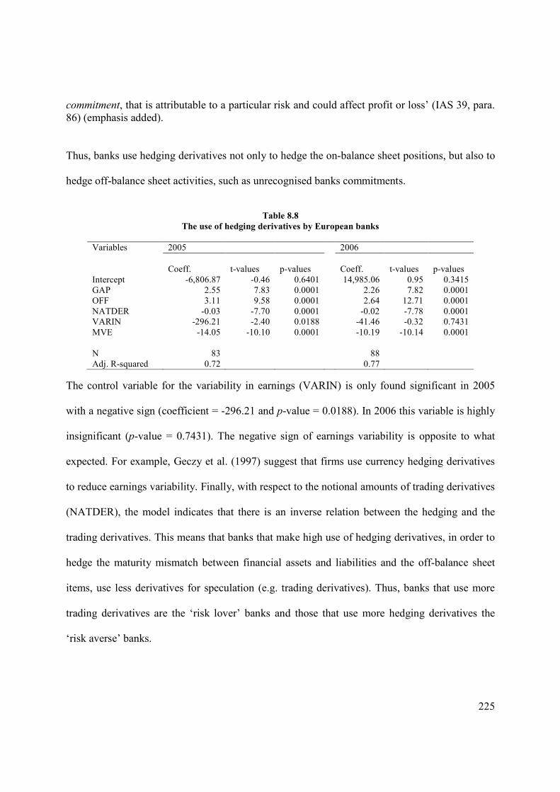
225

commitment, that is attributable to a particular risk and could affect profit or loss’ (IAS 39, para. 86) (emphasis added). Thus, banks use hedging derivatives not only to hedge the on-balance sheet positions, but also to

hedge off-balance sheet activities, such as unrecognised banks commitments.

Table 8.8

The use of hedging derivatives by European banks

Variables 2005 2006

Coeff. t-values p-values Coeff. t-values p-values

Intercept -6,806.87 -0.46 0.6401 14,985.06 0.95 0.3415 GAP 2.55 7.83 0.0001 2.26 7.82 0.0001 OFF 3.11 9.58 0.0001 2.64 12.71 0.0001

NATDER -0.03 -7.70 0.0001 -0.02 -7.78 0.0001 VARIN -296.21 -2.40 0.0188 -41.46 -0.32 0.7431

MVE -14.05 -10.10 0.0001 -10.19 -10.14 0.0001

N 83 88 Adj. R-squared 0.72 0.77

The control variable for the variability in earnings (VARIN) is only found significant in 2005

with a negative sign (coefficient = -296.21 and p-value = 0.0188). In 2006 this variable is highly

insignificant (p-value = 0.7431). The negative sign of earnings variability is opposite to what

expected. For example, Geczy et al. (1997) suggest that firms use currency hedging derivatives

to reduce earnings variability. Finally, with respect to the notional amounts of trading derivatives

(NATDER), the model indicates that there is an inverse relation between the hedging and the

trading derivatives. This means that banks that make high use of hedging derivatives, in order to

hedge the maturity mismatch between financial assets and liabilities and the off-balance sheet

items, use less derivatives for speculation (e.g. trading derivatives). Thus, banks that use more

trading derivatives are the ‘risk lover’ banks and those that use more hedging derivatives the

‘risk averse’ banks.

226

8.5 Conclusion

This chapter discussed the findings of the value relevance of fair value disclosures and fair value

recognition of derivatives of European banks under IFRS. The first test examines fair value

disclosures for a number of banks’ financial assets and liabilities that according to IAS 39 are

recognised in amortized costs. These items are loans and advances, held-to-maturity investments,

deposit liabilities, and other debt. IAS 32 requires the disclosure of these items in fair values.

The second test investigates the market valuation of derivatives’ fair value recognition.

Overall, the results support the view that fair value of loans are value relevance incrementally to

amortized costs. In all of the empirical models (primary and alternative specification models) the

variable of loans is found significant with the expected positive sign. This finding is consisted

with the results of previous studies that also found fair value of loans significant over and above

their book values (Barth et al., 1996). Apart from loans, fair values of other debt (other than

deposits) are also found significant in explaining market values. Their sign is estimated to be

negative as predicted.

The coefficients of the other variables of interest: the fair value of held-to-maturity investments

and the fair value of deposits are found to be insignificant. The coefficient of held-to-maturity

investments was always negative and insignificant. The negative coefficient indicates that

investors penalize banks that hold held-to-maturity investments as they do not qualify for the

interest rate hedging relationship (IAS 39, para. 79) and due to the uncertainty surrounding

management’s intention and ability to hold these instruments to maturity. The variable of

deposits is also found insignificant in most of the models, however with the expected negative

227

sign. A plausible explanation is the restriction imposed by IAS 39 that the fair value of a liability

with a demand feature can not be less than the amount payable on demand (IAS 39, para. 49).

This restriction forced many banks to equal the fair value of demand deposits with their carrying

amounts.

The chapter also provided evidence that investors assign lower coefficient to the fair value of

loans of those banks that hold low capital adequacy ratios and domicile in Weak enforcement

rule countries. Previous studies provide evidence that banks with low capital adequacy ratios

have more incentives to manipulate fair value estimates of loans (Barth et al., 1996). This study

extended this literature by relating banks’ incentives to manipulate fair values to countries

enforcement rules. In particular, it is argued that the latitude of banks to manipulate fair values

depends on country-specific institutional factors, such as the ability of each country to enforce its

rules. Thus, banks domiciled in Weak enforcement rule countries have more freedom to

manipulate fair values than banks domiciled in Strong enforcement rule countries. Countries

classified into Weak enforcement and Strong enforcement rule countries based on the rule of law

scores provided by Kaufmann et al. (2009).

The control variables supported the findings of previous studies. Specifically, core deposit

intangible (CORE) is found positive and significant (Barth et al., 1996). This result supports the

view that investors consider core deposits as having a positive impact on banks market values.

This is logical given the fact that core deposits proxy for the long-term relationship of banks with

their customers. Non-performing loans (NPL) had a negative impact on the market value of

equity (Beaver et al., 1989). Although non-performing loans do not necessarily indicate

228

impairment of these loans, they do indicate the level of banks’ default risk. The variable that

controlled for interest rate risk: the maturity gap of interest-sensitive assets and liabilities (GAP)

was found significant with the expected negative coefficient. European banks in the sample were

‘asset sensitive’ (i.e. interest-sensitive assets exceeded interest-sensitive liabilities). Given the

fact that interest rates were in an upward trend during 2005 – 2006 (see, Figure 6.1), the value of

net interest-sensitive assets decreased. Consistent with Venkatachalam (1996) and Eccher et al.

(1996), the coefficient of notional amounts of derivatives (NADER) is estimated to be negative.

This result indicates that the higher the involvement of a bank in derivative contracts the lower

its marker value of equity.

Results regarding derivatives indicate that the fair values of derivatives’ recognition (trading and

hedging derivatives) are value relevant over and above their notional amounts in most of the

empirical models. Investors consider fair value of derivatives as providing additional information

content to the notional amounts of derivatives. Although notional amounts of derivatives provide

the magnitude of derivative contracts, they do not provide the current values of these contracts,

which is what fair values represent. Fair values can aid investors to conclude on whether

derivatives are a value-added activity for banks or an activity that increases the overall risk of

banks. These findings are consistent with the results reported by Venkatachalam (1996) who

found the fair values of derivative disclosures value relevant incrementally to their notional

amounts. Moreover, they are consistent with the results of Ahmed et al. (2006) that they found

value relevant the recognised fair values of derivatives.

229

The chapter also provided evidence that the market assigns lower coefficient to derivatives’ fair

value estimates of banks with high earnings volatility. As predicted, banks with high earnings

volatility have more incentives to manipulate the fair value estimates of derivatives in order to

smooth earnings (Barton, 2001). However, the latitude of banks to manipulate fair value

estimates will depend again on the ability of countries to enforce their rules. Hence, the market

will assign lower coefficient to banks with high earnings volatility that also domicile in Weak

enforcement rule countries. However, this result holds only for trading derivatives but not for

hedging derivatives. Further analysis revealed that banks use hedging derivatives for their

primary purpose that is to hedge the maturity gap of interest-sensitive assets and liabilities.

230

Chapter 9: Findings on the Cost of Equity Capital

9.1 Introduction

This chapter provides the empirical results of the impact of the mandatory adoption of IFRS on

banks’ CE. The univariate analysis involves comparisons between the level of CE for the three

years before the official adoption of IFRS in 2005 and the level of CE for the first three years

after their adoption. The results of the univariate analysis are provided for the full sample, and

separately, i) for banks with low analyst following vs. high analyst following, ii) for banks

domiciled in ‘Anglo-Saxon’ countries vs. ‘Continental’ countries, and iii) for banks domiciled in

‘Strong Enforcement rule’ countries vs. ‘Weak Enforcement rule’ countries.

Given the fact that the univariate analysis does not take into account other factors (apart from the

IFRS adoption) that have affected the CE, results are also provided from a multivariate model

that controls for a number of risk-related variables. The chapter also reports the findings from a

number of additional tests in order to assess whether the effects on the CE vary with the level of

analysts following (low following vs. high following), the countries’ legal enforcement

environment (Weak enforcement rule vs. strong enforcement rule countries), and the

classification of the national accounting standards (Continental vs. Anglo-Saxon accounting

standards). Finally, findings are also provided under alternative model specifications for

robustness.

This chapter is organized as follows: Section 9.2 presents the descriptive statistics, Section 9.3

discusses the findings of the univariate analysis, Section 9.4 reports the findings of the primary

231

multivariate models as well as the findings of the additional analysis which relates to the

influence on the CE of: the level of analysts following; the countries’ enforcement rules, and

national accounting standards. Section 9.5 reports the findings of the robustness tests, and


9.2 Descriptive statistics

The number of banks in the sample of the cost of equity tests differs substantially from that of

the value relevance test due to the availability of some variables. For example, for the cost of

equity test, analysts’ forecasted earnings per share (provided via I/B/E/S) was a vital input in the

calculations of the CE. The fact that analysts cover only a small fraction of the population of this

thesis results in a smaller sample for the cost of equity test (88 banks) as compared to the sample

of the value relevance test (110 banks in 2006).

Panel A in Table 9.1 reports the descriptive statistics for the independent continuous variables

and Panel B for the dummy variables. The results indicate that the sample includes different

types of bank sizes with the smallest bank having a value of total assets (market value of equity)

of 317.00 million (29.42 million) and the biggest bank a value of 2.64 trillion (154.21 billion).

The average ASSET is 208,710.80 million and the median 43,599.89 million, indicating that the

series of ASSET is positively skewed. The same observation can be made for MVE with average

and median values of 14,779.71 million and €5,290.09 million, respectively.

The average book value of net loans is higher than the average book value of deposits which

gives an average LD ratio of 1.78. The LD ratio combined with the Long-term debt to Equity

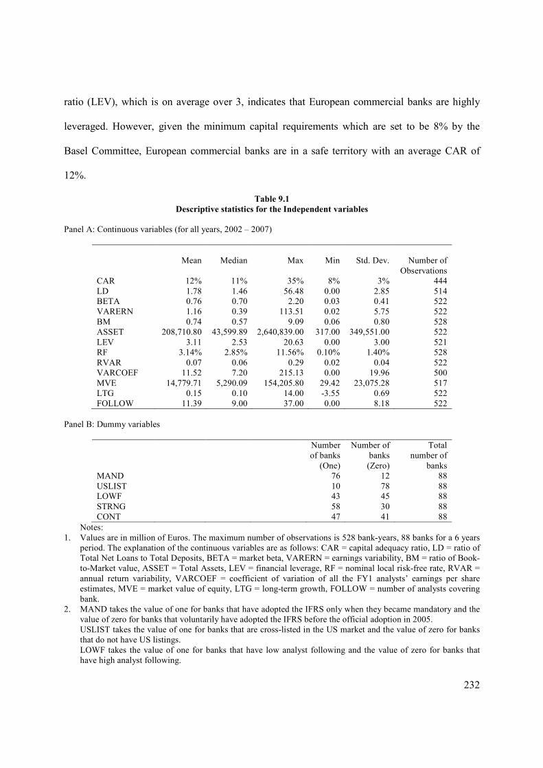
232

ratio (LEV), which is on average over 3, indicates that European commercial banks are highly

leveraged. However, given the minimum capital requirements which are set to be 8% by the

Basel Committee, European commercial banks are in a safe territory with an average CAR of

12%.

Table 9.1

Descriptive statistics for the Independent variables

Panel A: Continuous variables (for all years, 2002 – 2007)

Mean Median Max Min Std. Dev. Number of

Observations CAR 12% 11% 35% 8% 3% 444

LD 1.78 1.46 56.48 0.00 2.85 514 BETA 0.76 0.70 2.20 0.03 0.41 522 VARERN 1.16 0.39 113.51 0.02 5.75 522

BM 0.74 0.57 9.09 0.06 0.80 528 ASSET 208,710.80 43,599.89 2,640,839.00 317.00 349,551.00 522

LEV 3.11 2.53 20.63 0.00 3.00 521 RF 3.14% 2.85% 11.56% 0.10% 1.40% 528

RVAR 0.07 0.06 0.29 0.02 0.04 522 VARCOEF 11.52 7.20 215.13 0.00 19.96 500

MVE 14,779.71 5,290.09 154,205.80 29.42 23,075.28 517 LTG 0.15 0.10 14.00 -3.55 0.69 522 FOLLOW 11.39 9.00 37.00 0.00 8.18 522

Panel B: Dummy variables

Number of banks

(One)

Number of banks

(Zero)

Total number of

banks MAND 76 12 88

USLIST 10 78 88 LOWF 43 45 88

STRNG 58 30 88 CONT 47 41 88

Notes:

1. Values are in million of Euros. The maximum number of observations is 528 bank-years, 88 banks for a 6 years period. The explanation of the continuous variables are as follows: CAR = capital adequacy ratio, LD = ratio of Total Net Loans to Total Deposits, BETA = market beta, VARERN = earnings variability, BM = ratio of Book-to-Market value, ASSET = Total Assets, LEV = financial leverage, RF = nominal local risk-free rate, RVAR =

annual return variability, VARCOEF = coefficient of variation of all the FY1 analysts’ earnings per share estimates, MVE = market value of equity, LTG = long-term growth, FOLLOW = number of analysts covering

bank. 2. MAND takes the value of one for banks that have adopted the IFRS only when they became mandatory and the

value of zero for banks that voluntarily have adopted the IFRS before the official adoption in 2005. USLIST takes the value of one for banks that are cross-listed in the US market and the value of zero for banks that do not have US listings.

LOWF takes the value of one for banks that have low analyst following and the value of zero for banks that have high analyst following.

233

STRNG takes the value of one for banks that domicile in strong enforcement rule countries and zero for banks

that domicile in weak enforcement rule countries. CONT takes the value of one for banks that used to follow Continental accounting standards, before the mandatory adoption of IFRS, and zero for banks that used to follow Anglo-Saxon accounting standards.

The average BETA of the sample is 0.76. This number indicates that share prices of European

commercial banks fluctuate less to the variations of the market index DJ STOXX 600. The

alternative measure of market variability (RVAR) is found to be 0.07 (or 7%). The higher it is

the higher the risk of a bank. The variables that control for earnings variability, the VARERN

and the VARCOEF have a value of 1.16 and 11.52, respectively. Higher values for these

variables indicate higher variability in banks’ earnings. The below the unity BM variable reveals

that commercial banks are priced quite above their book values with an average book-to-market

ratio of 0.74. The average long-term growth (LTG) of earnings per share is approximately 15%,

while on average each European commercial bank in the sample is covered by 11 analysts.

Finally, the average risk-free rate (RF) is found 3.14% implying an average risk premium for

commercial banks of 6.26% (calculated as the average CE, 9.40%, from Table 9.3 below, less

the risk-free rate of 3.14%).

Panel B in Table 9.1 presents the descriptive statistics of the dummy variables which take the

value of ‘one’ or ‘zero’. MAND shows that only 12 out of 88 banks have voluntarily adopted the

IFRS before they became mandatory and USLIST reveals that only 10 banks have US listing.

STRNG indicates that most of the sample banks domicile in strong enforcement rule countries

(58 banks); in contrast, CONT shows that there is no material difference between the number of

banks from Continental countries (47) and the number of banks from Anglo-Saxon reporting

countries (41). No material difference can also be observed between banks with low and high

234

analyst following (e.g., 43 banks with low analyst following and 45 banks with high analyst

following).

Table 9.2 presents the descriptive statistics of the independent variables by country. The UK is

the country with the largest banks on average when the criterion of size is the market value of

equity (MVE). The average MVE for UK commercial banks is approximately €41.63 billion.

However, when the criterion of size is the variable of total assets (ASSET), French banks have

an average of €661.13 billion, while the UK banks fell in the second position, with an average of

482.18 billion. The countries with the smallest banks are Norway and Poland (in terms of MVE).

Germany is the country with the most sensitive banks to market volatilities as indicated by the

high values of BETA (1.30) and the RVAR (11%). It is also the country with the most leveraged

banks as it holds an average of 3.60 loans-to-deposits ratio (LD) and an average of 7.61 long-

term debt to equity ratio (LEV). The earnings volatility variables (VARERN and VARCOEF)

indicate again that Germany is the country with the most earnings volatile banks.

All countries in the sample hold a capital adequacy ratio well above the minimum capital

requirements of 8% imposed by the Basel Committee. Commercial banks in Switzerland

experience the highest CAR of 20%. All the remaining countries have a CAR equal or below the

13%. Regarding, the LTG variable, Netherland, Poland, and Greece are the three countries with

the highest future potential growths. Finally, the country with the lowest risk-free rates is

Switzerland with 0.87% value. On the other hand the country with the highest risk-free rates is

Hungary with 8.36% value.

23

5

Table 9.2

Descriptive statistics for the continuous independent variables – by Country

Number

of banks

CAR

LD

BETA VARERN

BM

ASSET

LEV

RF

RVAR

VARCOEF

MVE

LTG

FOLLOW

Au

stri

a 1

11

%

1.2

3

0.4

3

0.3

9

0.5

0

15

3,7

19

.20

5.4

6

2.8

8%

0.0

5

7.2

6

9,5

56.9

3

0.1

9

12

.66

Bel

giu

m

4

12

%

1.0

5

1.0

4

0.5

6

0.7

6

35

2,8

09

.20

2.6

6

2.8

1%

0.0

6

10

.73

20,4

04

.54

0.1

5

11

.04

Cze

ch R

epu

bli

c 1

13

%

1.0

2

0.6

3

1.6

9

0.4

0

17

,856

.66

0.4

6

2.3

7%

0.0

7

7.7

7

3,6

56.2

8

0.0

7

8.5

0

Den

mar

k

5

13

%

1.5

0

0.3

3

3.1

2

0.6

9

69

,806

.72

2.3

4

2.9

1%

0.0

5

7.1

9

4,4

73.3

7

0.1

4

5.2

6

Fin

lan

d

2

13

%

2.6

9

0.6

0

0.4

3

0.6

8

26

,468

.17

2.8

8

2.7

0%

0.0

6

10

.75

3,9

91.2

2

0.0

3

6.8

3

Fra

nce

5

10

%

1.1

9

0.8

4

0.4

2

0.7

8

66

1,1

33

.10

1.5

5

2.7

6%

0.0

6

8.6

6

29,3

49

.27

0.1

1

16

.66

Ger

man

y

6

12

%

3.6

0

1.3

0

4.0

1

0.9

1

17

7,8

56

.20

7.6

1

2.7

0%

0.1

1

41

.77

5,8

87.1

7

-0.0

4

11

.33

Gre

ece

5

12

%

1.1

5

0.7

1

0.9

3

0.4

2

38

,219

.53

1.5

5

2.7

9%

0.0

8

11

.76

5,5

71.8

3

0.2

4

11

.23

Hu

ngar

y

1

13

%

0.9

9

0.6

9

0.4

1

0.3

4

20

,411

.80

1.1

1

8.3

6%

0.0

8

5.1

8

5,8

60.8

2

0.1

4

7.8

3

Irel

and

4

11

%

1.5

9

0.6

3

0.3

6

0.4

9

88

,560

.25

3.8

0

2.7

0%

0.0

6

3.9

7

9,3

10.2

8

0.1

0

11

.54

Ital

y

10

12

%

2.3

8

0.8

1

0.3

9

0.7

7

13

6,5

70

.60

3.3

8

2.6

9%

0.0

6

13

.37

11,8

10

.50

0.1

5

11

.64

Net

her

land

4

12

%

1.1

3

1.0

5

0.9

1

0.5

8

40

9,4

65

.10

2.1

8

2.7

6%

0.0

9

14

.20

22,8

90

.54

0.6

7

13

.83

No

rway

7

11

%

1.7

3

0.3

8

0.4

7

2.1

8

21

,587

.67

3.8

5

3.8

1%

0.0

6

7.7

5

1,4

31.8

9

-0.0

2

4.1

9

Pola

nd

4

14

%

1.0

2

0.6

2

6.6

2

0.4

0

13

,941

.11

1.2

3

5.4

7%

0.0

9

10

.31

3,4

44.3

5

0.5

1

5.6

2

Port

ugal

3

11

%

1.6

9

0.4

3

0.2

4

0.5

0

51

,844

.12

5.3

3

2.7

6%

0.0

6

9.9

0

5,1

58.6

5

0.0

9

8.8

8

Spai

n

8

11

%

1.7

0

0.6

3

0.2

5

0.4

3

14

7,3

98

.80

3.0

0

2.6

8%

0.0

6

7.7

5

16,1

12

.39

0.1

5

13

.12

Sw

eden

4

10

%

2.2

3

0.7

9

0.2

5

0.6

0

19

8,0

53

.50

3.6

3

2.8

8%

0.0

5

6.2

4

13,2

92

.33

0.0

5

17

.41

Sw

itze

rlan

d

4

20

%

0.7

8

1.1

5

0.6

5

0.6

1

30

2,9

62

.30

0.9

9

0.8

7%

0.0

8

15

.56

22,1

30

.77

0.1

2

10

.54

UK

1

0

12

%

2.3

3

0.8

2

0.3

5

0.5

1

48

2,1

84

.20

3.0

0

4.4

9%

0.0

6

6.2

9

41,6

31

.77

0.0

9

16

.90

All

88

12

%

1.78

0.76

1.16

0.74

208,710.80

3.11

3.14%

0.07

11.52

14,779.71 0.15

11.39

Note

s:

Val

ues

of

AS

SE

T,

and

MV

E a

re i

n m

illi

on o

f E

uro

s. C

AR

= c

apit

al a

deq

uac

y r

atio

, L

D =

rat

io o

f T

ota

l N

et L

oan

s to

Tota

l D

eposi

ts,

BE

TA

= m

arket

bet

a,

VA

RE

RN

= e

arnin

gs

var

iab

ilit

y,

BM

= r

atio

of

Bo

ok-t

o-M

arket

val

ue,

AS

SE

T =

To

tal

Ass

ets,

LE

V =

fin

anci

al l

ever

age,

RF

= n

om

inal

lo

cal

risk

-fre

e ra

te,

RV

AR

= a

nn

ual

ret

urn

var

iabil

ity,

VA

RC

OE

F =

co

effi

cien

t of

var

iati

on

of

all

the

FY

1 a

nal

ysts

’ ea

rnin

gs

per

sh

are

esti

mat

es,

MV

E =

mar

ket

val

ue

of

equit

y,

LT

G =

lo

ng-t

erm

gro

wth

, F

OL

LO

W =

nu

mb

er o

f an

alyst

s co

ver

ing b

ank.

236

Table 9.3 presents the descriptive statistics by year and by country for the average CE. Panel A

presents the classification of the average CE by year and Panel B by country. However,

Appendix C also presents the results for each of the four CE methods (Gebhardt et al., 2001;

Claus & Thomas, 2001; Gode & Mohanram, 2003; and Easton, 2004). The number of

observations in Panel A represents the number of banks included in each year and the number of

observations in Panel B represents the number of bank-years observations. The calculations of

the CE are as of the last date of each year (31st December).

Table 9.3

Descriptive statistics for the Cost of Equity Capital

Panel A: By Year Mean Median Max Min Std. Dev. Number of

Observations

2002 11.35% 10.45% 24.88% 6.08% 3.47% 88 2003 9.33% 9.17% 15.74% 1.11% 2.43% 88

2004 9.42% 9.05% 27.72% 5.70% 2.68% 88 2005 8.44% 8.47% 13.12% 5.01% 1.49% 88

2006 8.54% 8.63% 12.69% 4.94% 1.50% 88 2007 9.30% 9.42% 14.28% 5.64% 1.73% 88

All 9.40% 9.15% 27.72% 1.11% 2.51% 528

Panel B: By Country (for all years, 2002 – 2007)

Mean Median Max Min Std. Dev. Number of Observations

Austria 10.25% 10.26% 11.49% 9.06% 0.77% 6 Belgium 8.94% 9.28% 11.56% 5.64% 1.39% 24

Czech Republic 7.78% 7.62% 11.48% 5.01% 2.09% 6 Denmark 9.30% 8.64% 24.88% 5.25% 3.63% 30 Finland 8.36% 7.87% 11.50% 6.17% 1.73% 12 France 9.70% 9.35% 14.98% 6.49% 1.82% 30 Germany 11.65% 9.95% 27.72% 5.91% 4.97% 36

Greece 10.94% 10.80% 13.99% 7.24% 1.38% 30 Hungary 10.10% 10.21% 11.05% 8.72% 0.92% 6 Ireland 9.50% 9.22% 12.66% 7.95% 1.22% 24 Italy 9.51% 9.42% 21.64% 1.11% 2.92% 60

Netherland 9.00% 8.81% 12.72% 5.98% 1.79% 24 Norway 9.83% 9.52% 15.74% 7.03% 1.78% 42

Poland 10.89% 10.37% 16.91% 6.32% 3.21% 24 Portugal 8.49% 8.30% 10.91% 6.32% 1.12% 18 Spain 8.70% 8.81% 11.56% 5.67% 1.36% 48

Sweden 7.80% 7.65% 10.39% 6.41% 1.02% 24 Switzerland 8.18% 7.92% 11.94% 5.89% 1.57% 24

UK 8.62% 8.58% 11.80% 5.90% 1.36% 60

All 9.40% 9.15% 27.72% 1.11% 2.51% 528

237

The descriptive statistics indicate that the average CE has decreased from 2002 to 2005.

Specifically, the average CE is at the highest point at the first year of the sample in 2002 with a

value of 11.35%, and takes the lowest value in 2005 where the IFRS became mandatory, 8.44%.

After 2005 the CE started to increase again and in 2007 returned above nine percent at 9.30%,

however quite below the highest value observed in 2002. Hence, the analysis indicates that the

CE is lower for the post-IFRS period than the pre-IFRS period. The results for the medians are

qualitative similar to the averages. Similar findings can also be observed for each of the four CE

methods (see, Appendix C).

The banks with the five highest average CE are those domiciled in Germany, 11.65%, Greece,

10.94%, Poland 10.89%, Austria, 10.25%, and Hungary, 10.10%. On the other hand, the banks

with the five lowest average CE are those domiciled in Czech Republic, 7.78%, Sweden, 7.80%,

Switzerland, 8.18%, Finland, 8.36%, and Portugal, 8.49%. German banks are found to hold the

highest average CE (11.65%) due to a number of extreme observations. The examination of the

medians, which are not affected by extreme values, reveals that German banks fall to the fifth

position with a median CE of 9.95%, quite below Greek banks with a median CE of 10.80%,

Polish banks with a median of 10.37%, Austrian banks with 10.26%, and Hungarian banks with

a median of 10.21%. The results of the medians for banks domicile in countries with the lowest

CE do not change materially from the averages. Findings from each of the four CE methods (see,

Appendix C) reveal that German banks hold the highest CE only under the Easton (2004)

method (i.e. 14.04%). For all other methods, although German banks still hold high CE are not in

the first position. Unexpectedly, banks domicile in Greece and Poland that are found to hold one

of the highest CE under the average CE, under the GLS method they hold one of the lowest CE

238

(Appendix C, Table C1). With respect to the other CE methods (see, Appendix C, Tables C2-C4),

both Greece and Poland hold high CE.

9.3 Univariate analysis

The univariate analysis involves the examination of the changes in the CE over the period, 2002

to 2007. Exhibit 9.1 lists all the hypotheses developed in section 7.2 relating to the cost of equity

tests.

Exhibit 9.1

List of hypotheses of the cost of equity tests

H6: The mandatory adoption of IFRS did not have any material impact on banks’ CE. H7: Banks with low analyst following experienced a higher reduction in their CE than banks with high analyst following. H8: Banks domiciled in ‘Continental’ countries experienced a higher reduction in their CE than banks domicile in ‘Anglo-Saxon’ countries. H9: Banks domiciled in ‘strong enforcement rule’ countries experienced a higher reduction in their CE than banks domiciled in ‘weak enforcement rule’ countries.

Table 9.4 shows the level of CE for these six years using four different methods (see, Section

7.3.1.), as well as the average of these methods. Figure 9.1 presents these data graphically. The

examination of the four CE methods (see columns GLS, CT, OJ, and PEG method in Table 9.4)

indicates that the CE has decreased from the pre-IFRS period to the post-IFRS period under all

methods. The GLS, the CT, and the PEG methods clearly reveal that the CE has slightly

increased again during 2007, which is also reflected in the average CE (rAVG). The only method

239

under which the CE is decreasing for the whole sample period is the OJ method. This method

gives the lowest CE estimates, 8.21%, whilst the method that gives the highest CE is the CT

method, which gives an average CE of 10.09%. The increase in the CE that is observed in 2007

can be attributed to the financial crisis of 2008 with the first signs of the crisis having emerged in

2007. That year a great number of financial institutions made huge losses in financial assets,

including subprime loans and CDOs.

Table 9.4

Cost of equity capital – Full Sample

Quarter

GLS method

CT Method

OJ Method

PEG Method

Average

N rGLS N rCT N rOJ N RPEG N rAVG

Pre-IFRS

2002 88 10.66% 88 11.71% 82 10.18% 84 12.61% 88 11.35% 2003 88 8.93% 87 10.02% 85 8.55% 80 10.16% 88 9.33%

2004 88 8.88% 87 9.98% 81 8.71% 76 10.40% 88 9.42%

Average

Post-IFRS

9.49% 10,57% 9.15% 11.06% 10.04%

2005 88 8.43% 87 9.04% 80 7.34% 74 8.93% 88 8.44% 2006 88 8.72% 88 9.24% 80 7.13% 72 8.79% 88 8.54% 2007 88 9.84% 88 10.54% 80 7.28% 71 9.12% 88 9.30%

Average 9.00% 9.61% 7.25% 8.95% 8.76%

All 528 9.24% 525 10.09% 488 8.21% 457 10.00% 528 9.40%

240

Figure 9.1

Cost of Equity Capital by Estimation Method

Table 9.5 reports the average CE for 2002 – 2007 for the different groups of banks that are used

in the testing of Hypotheses H7, H8 and H9, i.e., those banks that are followed by Low and High

number of analysts; those that are domiciled in Continental and Anglo-Saxon countries, and

those domiciled in Strong and Weak enforcement environments.

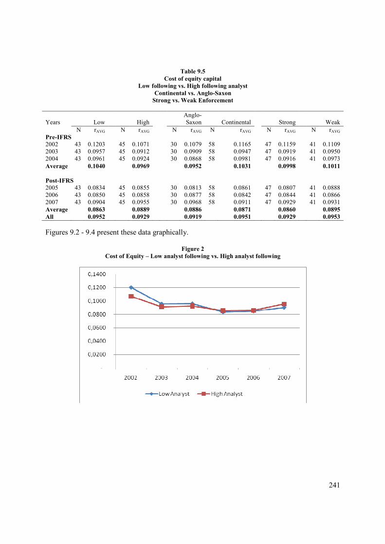
241

Table 9.5

Cost of equity capital

Low following vs. High following analyst

Continental vs. Anglo-Saxon

Strong vs. Weak Enforcement

Years

Low

High

Anglo-Saxon

Continental

Strong

Weak

N rAVG N rAVG N rAVG N rAVG N rAVG N rAVG

Pre-IFRS

2002 43 0.1203 45 0.1071 30 0.1079 58 0.1165 47 0.1159 41 0.1109 2003 43 0.0957 45 0.0912 30 0.0909 58 0.0947 47 0.0919 41 0.0950 2004 43 0.0961 45 0.0924 30 0.0868 58 0.0981 47 0.0916 41 0.0973

Average 0.1040 0.0969 0.0952 0.1031 0.0998 0.1011

Post-IFRS

2005 43 0.0834 45 0.0855 30 0.0813 58 0.0861 47 0.0807 41 0.0888 2006 43 0.0850 45 0.0858 30 0.0877 58 0.0842 47 0.0844 41 0.0866 2007 43 0.0904 45 0.0955 30 0.0968 58 0.0911 47 0.0929 41 0.0931

Average 0.0863 0.0889 0.0886 0.0871 0.0860 0.0895

All 0.0952 0.0929 0.0919 0.0951 0.0929 0.0953

Figures 9.2 - 9.4 present these data graphically.

Figure 2

Cost of Equity – Low analyst following vs. High analyst following

242

Figure 3

Cost of Equity – Continental vs. Anglo Saxon

Figure 4

Cost of Equity – Strong Enforcement vs. Weak Enforcement rule

243

Figure 9.2 indicates that before the mandatory adoption of IFRS banks with low analyst

following had higher CE than banks with high analyst following (e.g., in 2003 banks with low

analyst following had a CE of 9.57%, whilst banks with high analyst following had a CE of

9.12%). However, this discrepancy almost disappears after the mandatory adoption of IFRS in

2005. Figure 9.3 depicts the CE of banks domiciled in Continental and Anglo-Saxon countries.

On average, banks in the Anglo-Saxon group, for 2002 – 2007, had lower CE than banks in the

Continental group. However, during the post-IFRS period and especially in 2006 – 2007,

Continental banks experienced lower CE than Anglo-Saxon banks (e.g., in 2006 Continental

banks hold a CE of 8.42%, whilst Anglo-Saxon banks a CE of 8.77%). Figure 9.4 presents the

CE of banks domiciled in Strong enforcement vs. Weak enforcement rule countries. For most of

the post-IFRS period, banks domiciled in Strong enforcement rule countries experienced lower

CE.

Table 9.6 reports the difference-in-difference analysis for the CE around the mandatory adoption

period of IFRS. The data is taken from Tables 9.4 and 9.5, and are the average CE for the pre-

IFRS period and post-IFRS period for the full sample (Section A of the Table) and for the

different groups of interest (i.e., banks with high vs. low analyst following (Section B); banks

from Continental vs. Anglo-Saxon countries (Section C); and banks in Strong vs. Weak

enforcement environments, (Section D)).

244

Table 9.6

Difference-in-differences analysis for the cost of equity

Around the mandatory adoption period of IFRS

A) Full Sample

B) Low vs. High Analyst Following

C) Anglo-Saxon vs. Continental sample

D) Strong vs. Weak Enforcement sample

1. The CE data is that from the average CE (rAVG). 2. The three stars (***) indicate statistical significance of the differences in means, with p-values < 0.01 based

on two-tailed t-tests. The two stars (**) indicate statistical significance of the differences in means, with 0.01<p-value<0.05 based on two-tailed t-tests. The one star (*) indicates statistical significance of the

differences in means, with 0.1>p-value>0.05.

Pre-IFRS period Post-IFRS period Diff

Full sample, N = 528 bank-years

10.04% 8.76% -1.28%***


Low Analyst, N = 258 bank quarters

10.40%

8.63%% -1.77%***

High Analyst, N = 270 bank-quarters

9.69% 8.89% -0.80%***

Diff

0.71%

-0.26

-0.97%**


Continental, N = 348 bank quarters

10.31%

8.71% -1.60%***

Anglo-Saxon, N = 180 bank-quarters

9.52% 8.86% -0.66%

Diff

0.79%

-0.15%

-0.94%**

**


Strong, N = 282 bank-quarters

9.98% 8.60% -1.38%***

Weak, N = 246 bank quarters

10.11%

8.95% -1.16%***

Diff

-0.13%

-0.35%

-0.22%*

**

245

The results show that the average CE for the full sample of European commercial banks has

decreased from 10.04% in the pre-IFRS period to 8.76% in the post-IFRS period which is a

decrease of 1.28%. This difference is significant based on the equality test of means (p-

value<0.01). This finding rejects Hypothesis H6 that the mandatory adoption of IFRS did not

have a material impact on the CE.

Further results support Hypothesis H7 that banks with low analyst following experienced a

higher reduction in their CE after the mandatory adoption of IFRS (1.77% as compared to 0.80%

for high analyst following). The difference in the mean reductions (-0.97%) is significant at the

5% level of significance. Hypothesis H8 is also supported. but in the 10% level. Banks from

Continental countries experienced 1.60% reduction in their CE, whilst banks from Anglo-Saxon

countries experienced only a 0.66% reduction, which is a difference of 0.94%. This difference is

significant at the 10% level. With respect to Hypothesis H9, banks from Strong enforcement rule

countries experienced 1.38% reduction in their CE as opposed to a reduction of 1.16% that banks

in Weak enforcement rule countries experienced. This finding indicates a difference in the mean

reductions of 0.22, which based on the equality test of means is not significant.

9.4 Multivariate analysis


The univariate analysis above indicates that the CE of European commercial banks has decreased

after the mandatory adoption of IFRS. This section reports the findings of the multivariate

analysis which involves the testing of Equation (7.6):

246

CEit = γ0 + γ1 POSTit + γ2MANDit + γ3POST*MANDit + γ4CARit +γ5LDit + γ6BETAit + γ7VARERNit + γ8BMit + γ9

LOG(ASSET)it + γ10 LEV + γ11RFit + γ12USLISTit+ ∑18

k

kikCOUNTRYδ + ωit

Table 9.7 reveals that the issue of multicollinearity is not present among the independent

variables. The correlations between the independent variables are low with just a few values over

the fifty percent. Table 9.8 reports the primary findings that test Hypothesis H6. The explanatory

power of the model depends on the CE method. The GLS method gives the highest adjusted R-

squared, 68%, while the CT method provides the lowest adjusted R-squared, 31%. The adjusted

R-squared of the average CE method is 45%, indicating that the independent variables explain a

significant proportion of the variation of the dependent variable, the average CE. This

explanatory power is higher than that of Li (2010) but lower than that reported by Daske et al.

(2008). For example, Li (2010) reports an adjusted R-squared of 22% in her primary analysis,

while Daske et al. (2008) report an adjusted R-squared of around 80%.

The coefficient of the primary variable of interest, POST, is found significant with a negative

sign under all the CE estimation methods. This finding rejects the null Hypothesis H6 that the CE

has not been affected by the mandatory adoption of IFRS. The coefficient of POST indicates a

reduction of 111 to 383 basis points in the CE from the pre-IFRS period to the post-IFRS period,

depending on the method of the CE. The average reduction in the CE is 291 basis points.

This finding is in conformity with that of Daske et al. (2008), who reported a significant

reduction in the CE for a sample of worldwide firms from different industries. However, the

findings of that study held only when the researchers took into account the anticipation effect

(See, literature review, Chapter 5, Section 5.2.2.2).

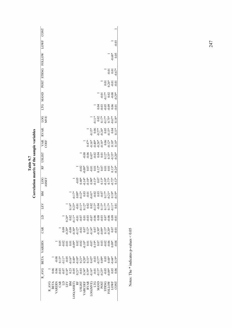
24

7

Table 9.7

Correlation matrix of the sample variables

R_

AV

G

BE

TA

V

AR

ER

N

CA

R

LD

L

EV

B

M

LO

G

AS

SE

T

RF

U

SL

IST

V

AR

C

OE

F

RV

AR

L

OG

M

VE

L

TG

M

AN

D

PO

ST

S

TR

NG

F

OL

LO

W

LO

WF

C

ON

T

R_

AV

G

1

B

ET

A

0.0

6

1

VA

RE

RN

0

.06

-0

.08

1

C

AR

-0

.03

0

.13*

0

.05

1

LD

-0

.07

-0

.11

*

-0.0

2

0.0

9

1

L

EV

0

.14*

-0

.05

-0

.01

-0

.20

*

0.2

4*

1

BM

0

.23

-0

.16

*

0.0

1

-0.0

9

0.0

2

0.1

4*

1

L

OG

(AS

SE

T)

-0.0

5

0.4

0*

-0

.09

*

-0.3

0*

-0.1

1*

0

.23*

-0.1

7*

1

RF

0

.21*

-0

.10

*

0.0

2

-0.1

2*

-0.0

1

-0.0

1

0.0

9*

-0

.05

1

U

SL

IST

-0

.03

0

.21*

-0

.02

-0

.02

-0

.07

-0

.11

*

-0.1

2*

0

.40*

-0.0

2

1

VA

RC

OE

F

0.3

4*

0

.20*

-0

.10

*

0.0

7

0.0

1

0.1

2*

0.0

3

-0.1

4*

-0.0

9*

-0.0

8

1

R

VA

R

0.3

9*

0

.31*

0

.01

0.1

2*

-0.0

3

0.0

2

-0.0

1

-0.1

8*

0.0

7

-0.0

6

0.4

7*

1

LO

G(M

VE

) -0

.16

*

0.4

5*

-0

.07

-0

.14

*

-0.0

7

0.0

2

-0.4

1*

0

.90*

-0.0

1

0.4

3*

-0.1

6*

-0.1

5*

1

L

TG

-0

.01

-0

.03

0

.19*

0.0

7

-0.0

6

-0.1

3*

-0.0

2

-0.1

3*

0.0

1

-0.0

2

-0.4

0*

0.0

6

-0.1

1*

1

MA

ND

-0

.13

*

-0.3

7*

0

.07

-0.3

0*

0.0

8

-0.0

4

0.0

3

0.0

7

0.1

2*

0.0

4

-0.2

6*

-0.2

7*

0.0

2

0.0

4

1

P

OS

T

-0.2

5*

0

.09*

0

.03

-0.0

9*

-0.0

3

0.1

3*

-0.0

7

0.1

3*

0.0

7

0.0

1

-0.1

6*

-0.2

4*

0.1

7*

-0

.03

-0

.01

1

ST

RN

G

-0.0

5

0.0

5

-0.0

2

0.1

3*

0.0

7

0.1

7*

0.1

7*

-0

.10

*

0.0

1

0.1

2*

0.0

6

0.0

5

-0.1

7*

-0

.05

-0

.17

*

0.0

1

1

F

OL

LO

W

-0.0

9*

0

.48*

-0

.06

-0

.20

*

-0.0

6

0.1

7*

-0.2

1*

0

.77*

0.0

1

0.3

5*

-0.1

2*

-0.1

5*

0.7

5*

-0

.09

0

.02

0

.26*

-0.0

1

1

LO

WF

0

.05

-0

.44

*

0.0

9*

0.0

7

0.0

9

-0.1

1*

0.1

9*

-0

.72

*

0.1

3*

-0.3

5*

0.1

0*

0.0

4

-0.6

7*

0

.06

-0.0

8

-0.0

1

0.0

1

-0.6

8*

1

C

ON

T

0.0

6

0.1

9*

-0

.04

-0

.01

-0

.01

0

.01

-0.1

9*

0

.12*

-0.2

4*

-0.2

0*

0.1

4*

0.1

1*

0.1

8*

-0

.01

-0

.29

*

-0.0

1

-0.6

7*

0

.05

-0.0

3

1

No

tes:

The

* i

ndic

ates

p-v

alu

es <

0.0

5

24

8

Table 9.8

Primary regression model

r G

LS

r C

T

r O

J

r PE

G

r A

VG

Var

iable

s C

oef

f.

t-val

ue

C

oef

f.

t-val

ue

C

oef

f.

t-val

ue

C

oef

f.

t-val

ue

C

oef

f.

t-val

ue

Inte

rcep

t 0

.04

31

3.2

411

***

0.0

075

0.3

110

***

0.0

995

2.8

800

***

0.0

714

1.8

444

***

0.0

723

3.5

531

***

P

OS

T

-0.0

11

1

-3.4

47

8***

-0.0

18

5

-3.1

60

7***

-0.0

35

0

-4.3

17

4***

-0.0

38

3

-4.5

78

9***

-0.0

291

-5.9

03

5***

M

AN

D

0.0

015

0.1

864

***

0.0

175

1.1

885

***

-0.0

33

5

-1.6

72

5***

-0.0

09

1

-0.3

71

0***

-0.0

117

-0.9

51

1***

M

AN

D*P

OS

T

0.0

058

1.6

991

***

0.0

058

0.9

338

***

0.0

230

2.6

784

***

0.0

239

2.6

770

***

0.0

164

3.1

175

***

C

AR

-0

.02

68

-1.0

54

8***

0.0

857

1.8

454

***

0.0

517

0.8

166

***

-0.0

02

0

-0.0

30

4***

0.0

273

0.7

020

***

L

D

-0.0

01

4

-2.4

09

0***

-0.0

04

6

-4.2

08

0***

-0.0

06

9

-4.6

38

0***

-0.0

07

3

-3.8

44

2***

-0.0

049

-5.3

45

0***

B

ET

A

0.0

070

2.9

963

***

0.0

023

0.5

504

***

-0.0

06

1

-1.0

33

0***

0.0

057

0.9

222

***

0.0

015

0.4

241

***

V

AR

ER

N

0.0

001

1.8

641

***

0.0

001

0.4

813

***

0.0

005

2.3

303

***

0.0

003

1.4

956

***

0.0

003

2.5

160

***

B

M

0.0

174

18

.283

3***

0.0

002

0.1

344

***

0.0

403

5.0

928

***

0.0

497

5.9

643

***

0.0

094

6.4

709

***

L

OG

(AS

SE

T)

0.0

001

0.1

817

***

0.0

028

2.1

746

***

-0.0

03

0

-1.6

10

0***

-0.0

01

3

-0.6

81

5***

-0.0

008

-0.7

87

3***

L

EV

0

.00

07

2.6

691

***

0.0

011

2.1

444

***

0.0

012

1.7

194

***

0.0

014

1.8

068

***

0.0

012

2.7

768

***

R

F

0.0

064

9.7

871

***

0.0

093

7.7

382

***

0.0

039

2.2

371

***

0.0

054

2.8

933

***

0.0

072

7.1

253

***

U

SL

IST

0

.00

29

1.2

562

***

0.0

015

0.3

526

***

0.0

074

1.2

480

***

0.0

001

0.0

204

***

0.0

042

1.1

755

***

C

oun

try d

um

mie

s In

clu

ded

In

clu

ded

In

clu

ded

In

clu

ded

In

clu

ded

N

4

44

44

4

42

2

39

0

44

4

A

dj.

R2

0.6

8

0.3

1

0.4

7

0.4

0

0.4

5

Th

e *** i

ndic

ates

p-v

alu

es <

0.0

1,

** i

ndic

ates

p-v

alu

es <

0.0

5,

and

* i

ndic

ates

p-v

alu

es <

0.1

0.

249

Under all CE methods, the interaction term, MAND*POST, is positive, which means that banks

that did not adopt the IFRS before 2005 (the year of mandatory adoption) experienced a lower

reduction in the CE as compared to banks that voluntarily adopted IFRS prior to 2005. However,

it is only significant under the OJ, the PEG, and importantly, under the AVG method. The

relevant coefficients reported in Table 9.8 were used to calculate the implied CE for the

mandatory and voluntary adopters, before and after the mandatory adoption of IFRS. The results

are presented in Table 9.9 using the average CE. Mandatory adopters experienced a CE of

0.0606 in the pre-IFRS period which has decreased by 0.0127 to 0.0479 in the post-IFRS period.

On the other hand, voluntary adopters had a CE of 0.0723 in the pre-IFRS period and a CE of

0.0432 in the post-IFRS period, implying a reduction of 0.029134. This result is opposite to the

findings of Li (2010) who found that mandatory adopters experienced a higher decrease in the

CE than voluntary adopters. However, consistent with Li (2010), the findings also show that the

difference in the CE between the mandatory adopters and the voluntary adopters in the pre-IFRS

period (0.0606 and 0.0723, respectively) has been eliminated in the post-IFRS period (0.0479

and 0.0432, respectively).

Table 9.9

CE of Mandatory and Voluntary adopters

based on the coefficients of the AVG method in Table 9.8

Pre-IFRS Post-IFRS Diff.

Mandatory Adopters 0.0606 0.0479 -0.0127***

Voluntary Adopters 0.0723 0.0432 -0.0291***

Diff. -0,0117 0,0047

*** indicates p-values < 0.01.

34 The CE estimates of the mandatory and the voluntary adopters have been calculated by the rAVG model in Table 9.8 by setting the two dummy variables of POST and MAND equal zero or one. For example, the CE of the

mandatory adopters in the pre-IFRS period (i.e. 0.0606), is calculated by setting the POST variable equal to zero and the MAND variable equal to one. Thus, the CE of this group is the sum of the intercept of the model (0.0723) with

the coefficient of MAND (-0.0117).

250

The findings in this thesis can be interpreted as follows. In contrast to voluntary adopters, firms

which adopted IFRS only when they became mandatory did not expect substantial benefits, such

as a reduction in the CE, and this is why they did not adopt IFRS earlier. In fact, as the post-

IFRS results show, the mandatory adoption of IFRS resulted in the elimination of the CE

advantage (a 0.0117 lower CE) they had during the pre-IFRS period over the voluntary adopters.

As Li (2010, p. 623) explains this finding is:

‘consistent with the assertion that a uniform set of high-quality accounting standards improves financial reporting convergence across the EU member states’.

The significance of the control variables vary depending on which CE estimation method is used.

The results of the bank specific variables are mixed. The capital adequacy ratio (CAR) is found

to be insignificant under all the CE methods. The LD variable is found to be significant in all CE

models with a negative coefficient. Mansur et al. (1993) predict a positive association between

this ratio and measures of risk (e.g. CE). As discussed in the methodology (Chapter 7, Section

7.3.2), a high net loans-to-deposits ratio should be associated with higher liquidity risk. However,

the negative coefficient of LD is supported by Wetmore (2004, p. 100) who argues that,

‘One argument in favor of high level of loan activity is banks securitize their loans thus reducing risk by removing them from the balance sheet. This permits them to make additional loans without having to increase the deposit base’.

However, whether the activity of securitization is a plausible explanation to support a negative

coefficient for the LD ratio is an empirical testable question.

BETA is found to be significant with the expected positive sign only under the GLS method

(coefficient = 0.0070, p-value = 0.0029). This finding indicates that banks with higher betas have

a higher risk which is reflected in their CE. The variable that controls for the variability of

251

earnings (VARERN) has a significant positive sign in two out of the five methods, the OJ

method (coefficient = 0.0005, p-value = 0.0203) and the average CE method (coefficient =

0.0003, p-value = 0.0122), indicating that the CE increases as the variability in earnings

increases.

In conformity with the literature, the BM ratio is found to be significant and positive (Daske,

2006; Gebhardt et al., 2001; Gode & Mohanram, 2003) while the variable controlling for size,

LOG(ASSET) is found significant (p-value = 0.0302) only under the CT method with a positive

sign. The significant coefficient (p-value = 0.0057 for the average CE method) of the leverage

ratio, LEV supports the view that there is a positive relationship between leverage and CE.

The variable of time-series variation in risk-free rates, the RF, is highly significant with a

positive sign under all CE methods. This finding suggests that the higher a country’s risk-free

rates are, the higher are the rates of return that investors demand from their investments in that

country, which is translated into higher CE for firms domiciled in that country. Finally, the US

cross-listing variable is insignificant under all methods.


This section reports the results of tests relating to Hypotheses: H7, H8 and H9. Additional analysis

examines whether the impact on the CE by the mandatory adoption IFRS vary with: i) analyst

following, ii) the classification of accounting standards, and iii) countries’ legal enforcement

rules.

252

The results on whether analyst following affects the impact of the IFRS on the CE are reported

on Table 9.10 (Hypothesis H7 in Chapter 7). The coefficient of POST is still significant with a

negative sign under all CE methods. This indicates again that the CE has decreased in the post-

IFRS period for the full sample. However, the coefficient of the interaction term, POST*LOWF,

is not found to be significant except under the GLS model. Thus, there is little support for

Hypothesis H7, that banks with low analyst following experienced lower reduction in their CE.

This finding contradicts the results of Botosan (1997) and Botosan & Plumlee (2002) who

reported a higher reduction in the CE of firms with low analyst following. However, with respect

to mandatory and voluntary adopters, results indicate that the three-way interaction term,

POST*MAND*LOWF, is significant and negative under two out of five CE methods (i.e. the

GLS and the CT method). This reveals that mandatory adopters with low analyst following had a

greater reduction in their CE after the mandatory adoption of IFRS than the voluntary adopters.

With respect to the other control variables, the results are similar to those relating to the primary

regression model (see Table 9.8). An exception is the LEV variable which is significant in less

models (GLS and AVG model) and the LOG(ASSET) which is insignificant under all models.

25

3

Table 9.10

Regression results based on analysts’ following

r G

LS

r C

T

r O

J

r PE

G

r A

VG

Var

iable

s C

oef

f.

t-val

ue

C

oef

f.

t-val

ue

C

oef

f.

t-val

ue

C

oef

f.

t-val

ue

C

oef

f.

t-val

ue

Inte

rcep

t 0

.04

60

3.2

153

***

0.0

205

0.7

786

***

0.0

402

1.0

827

***

0.0

430

1.0

264

***

0.0

570

2.5

824

***

P

OS

T

-0.0

17

3

-4.1

09

5***

-0

.02

54

-3.2

78

7***

-0.0

29

9

-2.8

08

7***

-0.0

41

7

-3.7

31

5***

-0.0

33

0

-5.0

733

***

M

AN

D

-0.0

03

9

-0.4

71

6***

0.0

176

1.1

516

***

-0.0

05

4

-0.2

62

3***

0.0

044

0.1

748

***

-0.0

03

2

-0.2

539

***

L

OW

F

-0.0

04

4

-0.6

42

3***

0.0

035

0.2

807

***

0.0

789

4.6

023

***

0.0

419

2.3

214

***

0.0

290

2.7

310

***

P

OS

T*M

AN

D

0.0

165

3.7

082

***

0.0

195

2.3

775

***

0.0

178

1.5

912

***

0.0

270

2.2

836

***

0.0

242

3.5

139

***

P

OS

T*L

OW

F

0.0

128

2.0

499

***

0.0

160

1.3

921

***

-0.0

15

0

-0.9

65

6***

0.0

058

0.3

598

***

0.0

073

0.7

648

***

M

AN

D*

LO

WF

0

.01

20

1.7

451

***

-0

.00

28

-0.2

20

2***

-0.0

73

4

-4.2

58

1***

-0.0

42

5

-2.3

45

2***

-0.0

24

5

-2.2

993

***

P

OS

T*M

AN

D*

LO

WF

-0

.02

40

-3.6

12

4***

-0

.03

05

-2.4

89

2***

0.0

127

0.7

567

***

-0.0

06

3

-0.3

56

0***

-0.0

16

7

-1.6

338

***

C

AR

-0

.03

58

-1.4

37

0***

0.0

721

1.5

698

***

0.0

743

1.1

935

***

0.0

105

0.1

555

***

0.0

272

0.7

078

***

L

D

-0.0

01

4

-2.3

90

3***

-0

.00

43

-4.0

37

4***

-0.0

06

6

-4.5

20

9***

-0.0

06

9

-3.6

03

4***

-0.0

04

7

-5.1

729

***

B

ET

A

0.0

079

3.2

653

***

0.0

007

0.1

678

***

-0.0

01

8

-0.2

93

6***

0.0

072

1.0

907

***

0.0

030

0.8

011

***

V

AR

ER

N

0.0

001

2.0

561

***

0.0

001

0.4

590

***

0.0

004

1.8

903

***

0.0

002

1.2

357

***

0.0

003

2.2

501

***

B

M

0.0

172

18

.587

***

0.0

002

0.1

525

***

0.0

393

4.9

579

***

0.0

486

5.7

074

***

0.0

094

6.5

805

***

L

OG

(AS

SE

T)

0.0

002

0.3

254

***

0.0

018

1.2

916

***

-0.0

00

7

-0.3

43

7***

-0.0

00

3

-0.1

36

3***

-0.0

00

3

-0.3

246

***

L

EV

0

.00

06

2.2

205

***

0.0

008

1.5

101

***

0.0

010

1.4

038

***

0.0

012

1.5

515

***

0.0

010

2.2

135

***

R

F

0.0

064

9.8

296

***

0.0

092

7.6

801

***

0.0

035

2.0

411

***

0.0

054

2.8

970

***

0.0

070

6.9

773

***

U

SL

IST

0

.00

25

1.0

758

***

0.0

013

0.3

089

***

0.0

024

0.4

148

***

-0.0

02

7

-0.4

39

8***

0.0

023

0.6

369

***

C

ou

ntr

y d

um

mie

s In

clu

ded

In

clu

ded

In

clu

ded

In

clu

ded

In

clu

ded

N

44

4

444

42

2

39

0

44

4

A

dj.

R2

0.7

0

0.3

3

0.5

0

0.4

1

0.4

8

Th

e *** i

ndic

ates

p-v

alu

es <

0.0

1,

** i

ndic

ates

p-v

alu

es <

0.0

5,

and

* i

ndic

ates

p-v

alu

es <

0.1

0.

254

The interaction term POST*CONT in Table 9.11 tests hypothesis H8. The significant and negative

coefficient indicates that, compared to banks domiciled in Anglo-Saxon countries, banks

domiciled in Continental countries experienced a higher reduction in their CE. This result provides

support for Hypothesis H8. The differences between the Anglo-Saxon accounting systems and

IFRS are regarded to be small which means that the benefits of adopting IFRS should be greater

for banks domiciled in countries with Continental accounting systems. Under the average CE

method, the negative coefficient of POST*CONT indicates that the CE of banks in Continental

countries decreased by 180 basis points more than the CE of banks in Anglo-Saxon countries. This

decrease ranges from 76 to 231 basis points depending on which CE method is used. The three-

way interaction term, POST*MAND*CONT, is significant and positive under the OJ, the PEG,

and the AVG method (e.g., for the AVG method, coefficient = 0.0157 and p-value = 0.0001). This

indicates that mandatory adopters domiciled in Continental countries experienced a lower

reduction in their CE after the mandatory adoption of IFRS than voluntary adopters.

Finally, the findings regarding the influence of countries’ enforcement rules support hypothesis H9

(Table 9.12). The interaction term POST*STRNG is significant and negative which suggests that

banks domiciled in strong enforcement countries have a higher reduction in their CE than banks

domiciled in weak enforcement countries. This finding is in conformity with the results of

previous studies, such as those of Li (2010). The reduction in the average CE is 136 basis points

for banks in weak enforcement countries and 371 basis points (136 + 235 basis points) for banks

in strong enforcement countries. The difference in the reduction of the CE varies from 79 to 341

basis points based on the CE method. The three-way interaction term, POST*MAND*STRNG,

gauges the difference in the reduction of CE between the mandatory adopters

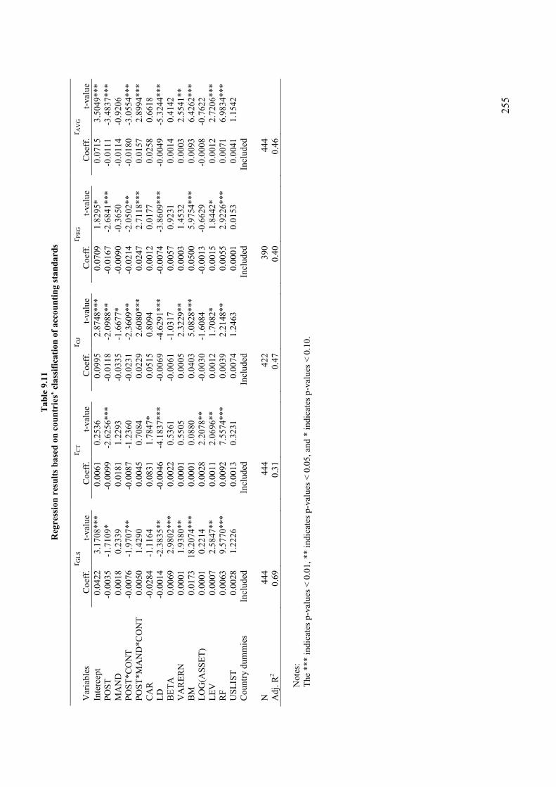
25

5

Table 9.11

Regression results based on countries’ classification of accounting standards

r G

LS

r C

T

r O

J

r PE

G

r A

VG

Var

iable

s C

oef

f.

t-val

ue

C

oef

f.

t-val

ue

C

oef

f.

t-val

ue

C

oef

f.

t-val

ue

C

oef

f.

t-val

ue

Inte

rcep

t 0

.04

22

3.1

708

***

0.0

061

0.2

536

***

0.0

995

2.8

748

***

0.0

709

1.8

295

***

0.0

715

3.5

049

***

P

OS

T

-0.0

03

5

-1.7

10

9***

-0.0

09

9

-2.6

25

6***

-0.0

11

8

-2.0

98

8***

-0.0

16

7

-2.6

841

***

-0.0

11

1

-3.4

83

7***

M

AN

D

0.0

018

0.2

339

***

0.0

181

1.2

293

***

-0.0

33

5

-1.6

67

7***

-0.0

09

0

-0.3

650

***

-0.0

11

4

-0.9

20

6***

P

OS

T*C

ON

T

-0.0

07

6

-1.9

70

7***

-0.0

08

7

-1.2

36

0***

-0.0

23

1

-2.3

60

9***

-0.0

21

4

-2.0

502

***

-0.0

18

0

-3.0

55

4***

P

OS

T*M

AN

D*C

ON

T

0.0

050

1.4

290

***

0.0

045

0.7

084

***

0.0

229

2.6

080

***

0.0

247

2.7

118

***

0.0

157

2.8

994

***

C

AR

-0

.02

84

-1.1

16

4***

0.0

831

1.7

847

***

0.0

515

0.8

094

***

0.0

012

0.0

177

***

0.0

258

0.6

618

***

L

D

-0.0

01

4

-2.3

83

5***

-0.0

04

6

-4.1

83

7***

-0.0

06

9

-4.6

29

1***

-0.0

07

4

-3.8

609

***

-0.0

04

9

-5.3

24

4***

B

ET

A

0.0

069

2.9

802

***

0.0

022

0.5

361

***

-0.0

06

1

-1.0

31

7***

0.0

057

0.9

231

***

0.0

014

0.4

142

***

V

AR

ER

N

0.0

001

1.9

380

***

0.0

001

0.5

505

***

0.0

005

2.3

229

***

0.0

003

1.4

532

***

0.0

003

2.5

541

***

B

M

0.0

173

18

.207

4***

0.0

001

0.0

880

***

0.0

403

5.0

828

***

0.0

500

5.9

754

***

0.0

093

6.4

262

***

L

OG

(AS

SE

T)

0.0

001

0.2

214

***

0.0

028

2.2

078

***

-0.0

03

0

-1.6

08

4***

-0.0

01

3

-0.6

629

***

-0.0

00

8

-0.7

62

2***

L

EV

0

.00

07

2.5

847

***

0.0

011

2.0

696

***

0.0

012

1.7

082

***

0.0

015

1.8

442

***

0.0

012

2.7

206

***

R

F

0.0

063

9.5

770

***

0.0

092

7.5

574

***

0.0

039

2.2

148

***

0.0

055

2.9

226

***

0.0

071

6.9

834

***

U

SL

IST

0

.00

28

1.2

226

***

0.0

013

0.3

231

***

0.0

074

1.2

463

***

0.0

001

0.0

153

***

0.0

041

1.1

542

***

C

ou

ntr

y d

um

mie

s In

clu

ded

In

clud

ed

Incl

ud

ed

Incl

ud

ed

Incl

ud

ed

N

44

4

44

4

42

2

39

0

44

4

A

dj.

R2

0.6

9

0.3

1

0.4

7

0.4

0

0.4

6

Note

s:

Th

e *** i

ndic

ates

p-v

alu

es <

0.0

1,

** i

ndic

ates

p-v

alu

es <

0.0

5,

and

* i

ndic

ates

p-v

alu

es <

0.1

0.

25

6

Table 9.12

Regression results based on countries’ enforcem

ent rules

r G

LS

r C

T

r O

J

r PE

G

r A

VG

Var

iable

s C

oef

f.

t-val

ue

C

oef

f.

t-val

ue

C

oef

f.

t-val

ue

C

oef

f.

t-val

ue

C

oef

f.

t-val

ue

Inte

rcep

t 0

.04

45

3.3

727***

0.0

121

0.5

048

***

0.1

012

2.9

307

***

0.0

737

1.9

094

***

0.0

752

3.7

339

***

P

OS

T

-0.0

06

6

-4.2

080

***

-0.0

13

6

-4.7

19

0***

-0.0

14

1

-3.4

93

0***

-0.0

13

5

-3.1

997

***

-0.0

13

6

-5.6

26

8***

M

AN

D

-0.0

01

0

-0.1

334

***

0.0

122

0.8

266

***

-0.0

36

7

-1.8

17

8***

-0.0

11

6

-0.4

716

***

-0.0

15

8

-1.2

85

0***

P

OS

T*S

TR

NG

-0

.00

79

-1.9

963

***

-0.0

14

1

-1.9

33

5***

-0.0

26

5

-2.6

50

9***

-0.0

34

1

-3.3

014

***

-0.0

23

5

-3.8

65

8***

P

OS

T*M

AN

D*S

TR

NG

0

.01

16

2.8

532***

0.0

181

2.4

284

***

0.0

307

2.9

656

***

0.0

316

2.8

844

***

0.0

264

4.2

445

***

C

AR

-0

.03

00

-1.1

855

***

0.0

783

1.6

938

***

0.0

498

0.7

860

***

-0.0

02

3

-0.0

344

***

0.0

231

0.5

980

***

L

D

-0.0

01

4

-2.4

010

***

-0.0

04

5

-4.1

94

9***

-0.0

06

9

-4.6

59

6***

-0.0

07

4

-3.8

825

***

-0.0

04

9

-5.3

88

0***

B

ET

A

0.0

070

2.9

919***

0.0

027

0.6

420

***

-0.0

06

0

-1.0

18

2***

0.0

065

1.0

487

***

0.0

019

0.5

477

***

V

AR

ER

N

0.0

001

2.0

645***

0.0

001

0.6

525

***

0.0

005

2.4

537

***

0.0

003

1.5

758

***

0.0

003

2.7

026

***

B

M

0.0

172

18.2

59

9***

0.0

001

0.0

318

***

0.0

387

4.8

573

***

0.0

476

5.6

830

***

0.0

092

6.3

951

***

L

OG

(AS

SE

T)

0.0

001

0.2

333***

0.0

027

2.1

698

***

-0.0

03

0

-1.6

32

8***

-0.0

01

5

-0.7

581

***

-0.0

00

8

-0.8

34

3***

L

EV

0

.00

07

2.4

170***

0.0

009

1.8

394

***

0.0

011

1.6

002

***

0.0

014

1.6

892

***

0.0

011

2.5

037

***

R

F

0.0

065

9.8

984***

0.0

094

7.8

499

***

0.0

045

2.5

241

***

0.0

062

3.3

159

***

0.0

075

7.4

922

***

U

SL

IST

0

.00

27

1.1

821***

0.0

011

0.2

775

***

0.0

073

1.2

348

***

0.0

001

0.0

163

***

0.0

040

1.1

257

***

C

ou

ntr

y d

um

mie

s In

clu

ded

In

clu

ded

In

clu

ded

In

clu

ded

In

clud

ed

N

44

4

44

4

42

2

39

0

44

4

A

dj.

R2

0.6

9

0.3

1

0.4

7

0.4

0

0.4

7

Th

e *** i

ndic

ates

p-v

alu

es <

0.0

1,

** i

ndic

ates

p-v

alu

es <

0.0

5,

and

* i

ndic

ates

p-v

alu

es <

0.1

0.

257

and the voluntary adopters. The results indicate that mandatory adopters domiciled in strong

enforcement rule countries had a lower reduction in their CE (for the AVG method, the

coefficient of POST*MAND*STRNG equals 0.0264, p-value = 0.0001). On the other hand,

voluntary adopters had a greater reduction in their CE when the IFRS became mandatory.

Overall, the results regarding the control variables, of the additional models, do not differ

materially from those of the primary regression model (Table 9.8). The BETA variable is found

significant only under the GLS method. The variability in earnings (VARERN) is found

significant with the expected positive sign in the GLS, the OJ and the AVG method. Again, the

ratio of Loans to Deposits (LD) is significant under all CE methods, however with the opposite

sign of the expected. The LEV variable is found significant in only one of the four CE methods

and in the average CE. Finally, the BM and the RF variables are also significant with the

expected signs, while the size variable, the natural logarithm of ASSET is significant in only one

of the CE methods.

9.5 Robustness tests


The primary findings reported above indicate that the CE has significantly decreased after the

mandatory adoption of IFRS in 2005. Based on the average CE estimates this reduction is 291

basis points (Table 9.8). In order to test whether these findings are affected by model

specification issues this section provides further evidence using alternative specification models.

258

Table 9.13 presents the results of the model that operationalizes a number of control variables in

a different way by using alternative variables (as explained in the methodology, Chapter 7, these

variables are: RVAR instead of BETA, VARCOEF instead of VARERN, LOG(MVE) instead of

LOG(ASSET)). The coefficient of POST is found to be significant and negative again (for the

AVG model, coefficient = -0.0186; p-value = 0.0001). The average CE model indicates a

reduction of 186 basis points from the pre to the post-IFRS period. The control variables, RVAR,

VARCOEF, and LOG(MVE), continue to be significant with the expected signs. Specifically,

the return variability (RVAR) is significant with a positive sign under the GLS (p-value =

0.0019), the PEG (p-value = 0.0002), and the AVG (p-value = 0.0053) models. The coefficient

of the alternative variable to earnings variability (VARCOEF) is significant and positive as

expected (e.g., for the AVG model, coefficient = 0.0002; p-value = 0.0001). The size variable,

LOG(MVE), is only significant under the OJ method with a coefficient of -0.0036 and a p-value

of 0.0118. The results with respect to all of the other variables are not different from those of the

primary regression model (Table 9.8).

Table 9.14 reports the findings of a model that controls for outliers by taking the natural

logarithms of the continuous independent variables. Under all the CE methods, the results show a

reduction in the CE after the mandatory adoption of IFRS. The coefficient of the POST variable

for the AVG method is -0.0276 with a p-value of 0.0001. A notable difference between the

model that controls for outliers and the primary estimation model in Table 9.8 is that the

explanatory power of the former model increases significantly up to 73% for the GLS model.

25

9

Table 9.13

Regression model using alternative control variables

r G

LS

r C

T

r O

J

r PE

G

r A

VG

Var

iable

s C

oef

f.

t-val

ue

C

oef

f.

t-val

ue

C

oef

f.

t-val

ue

C

oef

f.

t-val

ue

C

oef

f.

t-val

ue

Inte

rcep

t 0.0

539

4.4

873

***

0.0

328

1.5

182***

0.1

020

3.8

560

***

0.0

242

0.8

527

***

0.0

756

4.6

212

***

P

OS

T

-0.0

09

1

-2.6

20

3***

-0.0

19

7

-3.1

50

4***

-0.0

218

-2.9

07

0***

-0.0

118

-1.6

21

4***

-0.0

18

6

-3.9

20

2***

M

AN

D

-0.0

04

4

-0.5

39

7***

0.0

097

0.6

524***

-0.0

280

-1.5

69

0***

0.0

323

1.5

623

***

-0.0

11

8

-1.0

43

2***

M

AN

D*P

OS

T

0.0

053

1.4

614

***

0.0

075

1.1

497***

0.0

119

1.5

260

***

0.0

026

0.3

460

***

0.0

089

1.7

943

***

C

AR

-0

.03

23

-1.2

87

5***

0.0

495

1.0

956***

-0.0

153

-0.2

83

7***

-0.0

544

-1.0

18

9***

-0.0

13

3

-0.3

89

9***

L

D

-0.0

01

4

-2.3

23

6***

-0.0

04

5

-4.0

86

7***

-0.0

047

-3.5

80

5***

-0.0

063

-4.0

08

7***

-0.0

03

8

-4.4

93

1***

R

VA

R

0.0

685

3.1

310

***

0.0

561

1.4

228***

0.0

529

1.1

180

***

0.1

773

3.7

759

***

0.0

837

2.8

053

***

V

AR

CO

EF

-0

.00

01

-1.3

92

2***

-0.0

00

1

-1.9

48

9***

0.0

006

6.8

903

***

0.0

009

9.7

367

***

0.0

002

4.5

989

***

B

M

0.0

172

16

.550

4***

0.0

003

0.1

993***

0.0

174

2.2

359

***

0.0

316

4.1

388

***

0.0

080

5.6

965

***

L

OG

(MV

E)

-0.0

00

1

-0.1

70

8***

0.0

020

1.8

223***

-0.0

036

-2.5

29

8***

-0.0

004

-0.2

94

4***

-0.0

01

0

-1.2

37

0***

L

EV

0.0

008

2.7

732

***

0.0

015

2.7

610***

0.0

008

1.3

578

***

0.0

015

2.3

192

***

0.0

011

2.6

730

***

R

F

0.0

063

9.0

572

***

0.0

088

7.0

599***

0.0

033

2.0

963

***

0.0

042

2.6

910

***

0.0

061

6.4

191

***

U

SL

IST

0.0

055

2.3

795

***

0.0

047

1.1

204***

0.0

061

1.2

041

***

-0.0

001

-0.0

14

7***

0.0

052

1.6

455

***

C

ou

ntr

y d

um

mie

s In

clu

ded

In

clu

ded

In

clu

ded

In

clu

ded

In

clu

ded

N

4

30

43

0

41

4

382

43

0

A

dj.

R2

0.6

7

0.2

9

0.5

2

0.5

3

0.5

0

Note

s:

RV

AR

= i

s th

e an

nu

al r

etu

rn v

aria

bil

ity d

efin

ed a

s th

e st

and

ard

dev

iati

on

of

the

month

ly r

eturn

s at

yea

r en

d,

VA

RC

OE

F =

is

the

coef

fici

ent

of

var

iati

on

of

all

the

FY

1 a

nal

yst

s’ e

stim

ates

. It

is

a m

easu

re o

f sp

read

of

the

esti

mat

es i

n t

erm

s of

the

stan

dar

d d

evia

tio

n.

MV

E =

is

the

mar

ket

val

ue

of

equit

y a

nd

is

stat

ed i

n

mil

lio

ns

of

Euro

s. A

ll t

he

oth

er v

aria

ble

s ar

e d

efin

ed i

n T

able

9.8

. A

ltho

ugh t

he

mo

del

co

ntr

ols

fo

r th

e co

untr

y-e

ffec

t, t

he

table

do n

ot

pro

vid

es t

he

resu

lts

for

the

cou

ntr

y d

um

my v

aria

ble

s fo

r b

revit

y. T

he

**

* i

nd

icat

es p

-val

ues

< 0

.01

, ** i

ndic

ates

p-v

alu

es <

0.0

5, an

d *

in

dic

ates

p-v

alues

< 0

.10

.

260

The significance of most of the control variables is similar to the findings in Table 9.8.

VARERN, BM, and the RF are found significant with positive coefficients and LD has a

negative coefficient. For the first time the CAR is found significant with a negative sign,

however only under the GLS method (coefficient = -0.0093; p-value = 0.0049). As discussed in

Chapter 7 the higher it is the capital adequacy ratio the lower the CE which is supported by the

negative sign.

Table 9.15 reports the findings of the growth model which includes a proxy for the long-term

growth in earnings per share. Consistent with the findings of the primary model and the other

robustness tests, the coefficient of POST, shows that the CE has decreased after the mandatory

adoption of IFRS, under all CE methods. The results regarding the LTG are mixed. Although, it

is found significant under two CE methods, its coefficient is estimated to be positive under the

CT method (coefficient = 0.0098) and negative under the PEG method (coefficient = -0.0173).

Finally, Table 9.16 reports the results of the model that uses as the dependent variable the risk

premium instead of the CE. As explained in the methodology chapter (Chapter 7), this model

aims to test whether the results are sensitive to other measures of the required rate of return.

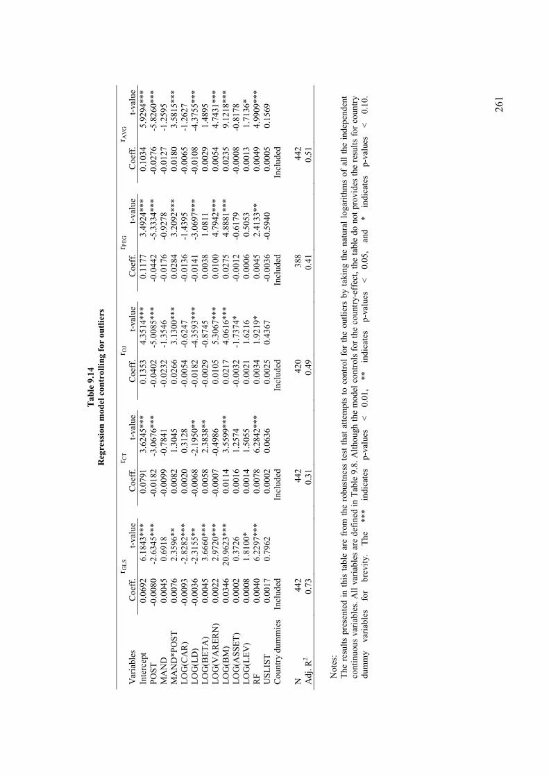
26

1

Table 9.14

Regression model controlling for outliers

r G

LS

r C

T

r O

J

r PE

G

r A

VG

Var

iable

s C

oef

f.

t-val

ue

C

oef

f.

t-val

ue

C

oef

f.

t-val

ue

C

oef

f.

t-val

ue

C

oef

f.

t-val

ue

Inte

rcep

t 0.0

692

6.1

843

***

0.0

791

3.6

245***

0.1

353

4.3

514

***

0.1

177

3.4

924

***

0.1

034

5.9

294

***

P

OS

T

-0.0

08

0

-2.6

34

5***

-0.0

18

2

-3.0

67

6***

-0.0

402

-5.0

08

5***

-0.0

442

-5.3

33

4***

-0.0

27

6

-5.8

26

0***

M

AN

D

0.0

045

0.6

918

***

-0.0

09

9

-0.7

84

1***

-0.0

232

-1.3

54

6***

-0.0

176

-0.9

27

8***

-0.0

12

7

-1.2

59

5***

M

AN

D*P

OS

T

0.0

076

2.3

596

***

0.0

082

1.3

045***

0.0

266

3.1

300

***

0.0

284

3.2

092

***

0.0

180

3.5

815

***

L

OG

(CA

R)

-0.0

09

3

-2.8

28

2***

0.0

020

0.3

128***

-0.0

054

-0.6

24

7***

-0.0

136

-1.4

39

5***

-0.0

06

5

-1.2

62

7***

L

OG

(LD

) -0

.00

36

-2.3

15

5***

-0.0

06

8

-2.1

95

0***

-0.0

182

-4.3

59

3***

-0.0

141

-3.0

69

7***

-0.0

10

8

-4.3

75

5***

L

OG

(BE

TA

) 0.0

045

3.6

660

***

0.0

058

2.3

838***

-0.0

029

-0.8

74

5***

0.0

038

1.0

811

***

0.0

029

1.4

895

***

L

OG

(VA

RE

RN

) 0.0

022

2.9

720

***

-0.0

00

7

-0.4

98

6***

0.0

105

5.3

067

***

0.0

100

4.7

942

***

0.0

054

4.7

431

***

L

OG

(BM

) 0.0

346

20

.962

3***

0.0

114

3.5

599***

0.0

217

4.0

616

***

0.0

275

4.8

881

***

0.0

235

9.1

218

***

L

OG

(AS

SE

T)

0.0

002

0.3

726

***

0.0

016

1.2

574***

-0.0

032

-1.7

37

4***

-0.0

012

-0.6

17

9***

-0.0

00

8

-0.8

17

8***

L

OG

(LE

V)

0.0

008

1.8

100

***

0.0

014

1.5

055***

0.0

021

1.6

216

***

0.0

006

0.5

053

***

0.0

013

1.7

136

***

R

F

0.0

040

6.2

297

***

0.0

078

6.2

842***

0.0

034

1.9

219

***

0.0

045

2.4

133

***

0.0

049

4.9

909

***

U

SL

IST

0.0

017

0.7

962

***

0.0

002

0.0

636***

0.0

025

0.4

367

***

-0.0

036

-0.5

94

0***

0.0

005

0.1

569

***

C

ou

ntr

y d

um

mie

s In

clu

ded

In

clu

ded

In

clu

ded

In

clu

ded

In

clu

ded

N

4

42

44

2

42

0

388

44

2

A

dj.

R2

0.7

3

0.3

1

0.4

9

0.4

1

0.5

1

Note

s:

Th

e re

sult

s p

rese

nte

d i

n t

his

tab

le a

re f

rom

th

e ro

bust

nes

s te

st t

hat

att

emp

ts t

o c

ontr

ol

for

the

outl

iers

by t

akin

g t

he

nat

ura

l lo

gar

ithm

s o

f al

l th

e in

dep

end

ent

conti

nu

ou

s var

iable

s. A

ll v

aria

ble

s ar

e d

efin

ed i

n T

able

9.8

. A

lth

ou

gh

th

e m

od

el c

ontr

ols

for

the

cou

ntr

y-e

ffec

t, t

he

table

do n

ot

pro

vid

es t

he

resu

lts

for

coun

try

du

mm

y

var

iab

les

for

bre

vit

y.

Th

e ***

indic

ates

p

-val

ues

<

0

.01

, **

indic

ates

p

-val

ues

<

0

.05

, an

d

*

indic

ates

p

-val

ues

<

0.1

0.

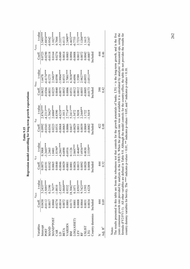
26

2

Table 9.15

Regression model controlling for long-term growth expectations

r G

LS

r C

T

r O

J

r PE

G

r A

VG

Var

iable

s C

oef

f.

t-val

ue

C

oef

f.

t-val

ue

C

oef

f.

t-val

ue

C

oef

f.

t-val

ue

C

oef

f.

t-val

ue

Inte

rcep

t 0

.04

30

3.2

435

***

0.0

073

0.3

068

***

0.0

992

2.8

763

***

0.0

632

1.6

478

***

0.0

723

3.5

495

***

P

OS

T

-0.0

11

2

-3.5

09

5***

-0.0

19

1

-3.2

68

5***

-0.0

34

3

-4.2

31

3***

-0.0

36

6

-4.4

17

4***

-0.0

290

-5.8

85

4***

M

AN

D

0.0

017

0.2

190

***

0.0

182

1.2

465

***

-0.0

34

1

-1.7

04

2***

-0.0

03

1

-0.1

27

5***

-0.0

118

-0.9

54

2***

M

AN

D*P

OS

T

0.0

060

1.7

657

***

0.0

065

1.0

401

***

0.0

223

2.6

068

***

0.0

225

2.5

483

***

0.0

164

3.1

027

***

C

AR

-0

.02

74

-1.0

81

0***

0.0

840

1.8

194

***

0.0

531

0.8

390

***

0.0

040

0.0

598

***

0.0

274

0.7

044

***

L

D

-0.0

01

4

-2.4

33

3***

-0.0

04

6

-4.2

66

1***

-0.0

06

8

-4.6

21

8***

-0.0

07

5

-3.9

90

4***

-0.0

049

-5.3

35

7***

B

ET

A

0.0

072

3.0

849

***

0.0

029

0.6

890

***

-0.0

06

5

-1.1

01

3***

0.0

052

0.8

515

***

0.0

014

0.4

113

***

V

AR

ER

N

0.0

001

0.9

532

***

-0.0

00

1

-0.6

91

6***

0.0

006

2.7

714

***

0.0

006

2.7

001

***

0.0

003

2.3

490

***

B

M

0.0

173

18

.304

2***

0.0

001

0.1

126

***

0.0

417

5.2

411

***

0.0

531

6.3

838

***

0.0

094

6.4

652

***

L

OG

(AS

SE

T)

0.0

001

0.1

071

***

0.0

026

2.0

697

***

-0.0

02

9

-1.5

47

2***

-0.0

01

2

-0.6

09

6***

-0.0

008

-0.7

75

5***

L

EV

0

.00

08

2.8

593

***

0.0

013

2.4

640

***

0.0

011

1.5

038

***

0.0

012

1.5

589

***

0.0

012

2.7

231

***

R

F

0.0

064

9.7

423

***

0.0

092

7.6

936

***

0.0

039

2.2

449

***

0.0

055

2.9

827

***

0.0

072

7.1

204

***

U

SL

IST

0

.00

31

1.3

393

***

0.0

020

0.4

830

***

0.0

069

1.1

722

***

-0.0

00

5

-0.0

95

5***

0.0

042

1.1

615

***

L

TG

0

.00

34

1.6

228

***

0.0

098

2.5

359

***

-0.0

08

2

-1.5

41

9***

-0.0

17

3

-3.0

51

1***

-0.0

007

-0.2

18

7***

C

oun

try d

um

mie

s In

clu

ded

In

clu

ded

In

clu

ded

In

clu

ded

In

clu

ded

N

4

44

44

4

42

2

39

0

44

4

A

dj.

R2

0.6

9

0.3

2

0.4

8

0.4

2

0.4

6

Note

s:

Th

e re

sult

s p

rese

nte

d i

n t

his

tab

le a

re f

rom

th

e ro

bu

stn

ess

test

th

at c

ontr

ols

for

the

gro

wth

pote

nti

als

of

ban

ks.

LT

G =

is

the

long-t

erm

gro

wth

, an

d i

s th

e fi

ve

yea

rs c

onse

nsu

s gro

wth

rat

e pro

vid

ed b

y a

nal

yst

s in

the

I/B

/E/S

. W

hen

th

e gro

wth

rat

e w

as n

ot

avai

lable

it

is c

alcu

late

d b

y a

nal

yst

s’ f

ore

cast

ed e

ps,

usi

ng t

he

form

ula

(F

Y2

/FY

1-1

).

All

oth

er v

aria

ble

s ar

e d

efin

ed i

n T

able

9.8

. A

lthou

gh

th

e m

od

el c

ontr

ols

for

the

cou

ntr

y-e

ffec

t, t

he

table

do

no

t p

rovid

es t

he

resu

lts

for

cou

ntr

y d

um

my v

aria

ble

s fo

r b

revit

y. T

he

**

* i

nd

icat

es p

-val

ues

< 0

.01

, ** i

ndic

ates

p-v

alu

es <

0.0

5, an

d *

in

dic

ates

p-v

alues

< 0

.10

.

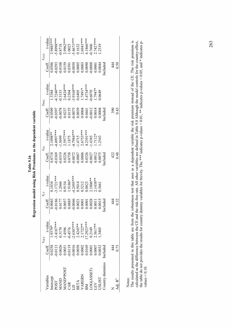
26

3

Table 9.16

Regression model using Risk Premiums as the dependent variable

r G

LS

r C

T

r O

J

r PE

G

r A

VG

Var

iable

s C

oef

f.

t-val

ue

C

oef

f.

t-val

ue

C

oef

f.

t-val

ue

C

oef

f.

t-val

ue

C

oef

f.

t-val

ue

Inte

rcep

t 0.0

258

1.9

379

***

0.0

043

0.1

834***

0.0

718

2.1

098

***

0.0

509

1.3

384

***

0.0

586

2.9

485

***

P

OS

T

-0.0

11

3

-3.4

18

7***

-0.0

18

6

-3.1

72

1***

-0.0

369

-4.4

99

7***

-0.0

397

-4.7

24

0***

-0.0

29

3

-5.8

99

8***

M

AN

D

0.0

026

0.3

170

***

0.0

177

1.2

044***

-0.0

319

-1.5

69

9***

-0.0

078

-0.3

15

3***

-0.0

10

8

-0.8

71

8***

M

AN

D*P

OS

T

0.0

051

1.4

596

***

0.0

057

0.9

154***

0.0

226

2.5

977

***

0.0

237

2.6

424

***

0.0

159

2.9

962

***

C

AR

-0

.01

19

-0.4

57

6***

0.0

885

1.9

186***

0.0

758

1.1

875

***

0.0

155

0.2

304

***

0.0

391

1.0

023

***

L

D

-0.0

01

6

-2.6

30

7***

-0.0

04

6

-4.2

49

5***

-0.0

072

-4.7

98

4***

-0.0

075

-3.9

16

8***

-0.0

05

0

-5.4

67

1***

B

ET

A

0.0

058

2.4

245

***

0.0

021

0.5

014***

-0.0

087

-1.4

71

5***

0.0

039

0.6

405

***

0.0

005

0.1

632

***

V

AR

ER

N

0.0

002

2.1

722

***

0.0

001

0.5

212***

0.0

006

2.6

753

***

0.0

004

1.7

491

***

0.0

003

2.6

941

***

B

M

0.0

169

17

.292

3***

0.0

001

0.0

823***

0.0

326

4.2

391

***

0.0

441

5.4

734

***

0.0

090

6.1

866

***

L

OG

(AS

SE

T)

0.0

001

0.2

149

***

0.0

028

2.1

806***

-0.0

027

-1.4

38

5***

-0.0

012

-0.6

07

0***

-0.0

00

8

-0.7

60

6***

L

EV

0.0

007

2.5

617

***

0.0

011

2.1

438***

0.0

012

1.7

112

***

0.0

014

1.7

947

***

0.0

001

2.7

427

***

U

SL

IST

0.0

032

1.3

405

***

0.0

015

0.3

661***

0.0

075

1.2

543

***

0.0

004

0.0

649

***

0.0

044

1.2

319

***

C

ou

ntr

y d

um

mie

s In

clu

ded

In

clu

ded

In

clu

ded

In

clu

ded

In

clu

ded

N

4

44

44

4

42

2

390

44

4

A

dj.

R2

0.7

3

0.3

2

0.4

8

0.4

3

0.5

0

Note

s:

Th

e re

sult

s p

rese

nte

d i

n t

his

tab

le a

re f

rom

th

e ro

bust

nes

s te

st t

hat

use

s as

a d

epen

den

t var

iable

th

e ri

sk p

rem

ium

in

stea

d o

f th

e C

E.

Th

e ri

sk p

rem

ium

is

calc

ula

ted a

s th

e dif

fere

nce

bet

wee

n t

he

CE

an

d t

he

risk

-fre

e ra

te.

All

oth

er v

aria

ble

s ar

e def

ined

in

Tab

le 9

.8 A

lth

ou

gh

th

e m

od

el c

ontr

ols

fo

r th

e co

un

try-e

ffec

t,

the

table

do

no

t p

rovid

es t

he

resu

lts

for

cou

ntr

y d

um

my v

aria

ble

s fo

r bre

vit

y. T

he

**

* i

nd

icat

es p

-val

ues

< 0

.01

, ** i

ndic

ates

p-v

alu

es <

0.0

5,

and

* i

ndic

ates

p-

val

ues

< 0

.10

.

264

Similar, to the models that use the CE as the dependent variable, the coefficient of POST

continues to be negative and significant. For example, for the AVG model the coefficient is -

0.0293 (p-value = 0.0001) indicating a reduction of 293 basis points after the mandatory

adoption of IFRS. Regarding the control variables the findings do not change materially from

those presented above (Table 9.8). CAR is still insignificant and LD is significant with a

negative sign. BETA and the size variable LOG(ASSET) are only significant under the GLS (p-

value = 0.0158) and the CT (p-value = 0.0298) method, respectively. Overall, the VARERN, the

BM, and the LEV variables continue to be significant and positive as before.


This section provides the robustness tests for the addition analysis performed under Section 9.4.2.

Four robustness tests are used for each of the additional tests. The robustness tests are similar to

the ones used in the primary analysis (See, Section 9.5.1).

Findings of the analyst following analysis are presented in Tables D1-D4 of Appendix D. Results

indicate again that banks with low analyst following do not experience lower reduction in their

CE after the mandatory adoption of IFRS than banks with high analyst following. The interaction

term POST*LOWF is insignificant almost in all the robustness tests and under all CE methods.

This finding do not supports Hypothesis H7. However, the POST variable that examines whether

the CE has decreased for the full sample after the mandatory adoption of IFRS is highly

significant in most of the models. For example, the coefficient of the AVG method for the model

that controls for outliers indicates that the CE has significantly decreased by 309 basis points (t-

stastistic = 4.8286, see Table D2 in Appendix D).

265

Tables D5-D8 in Appendix D report the robustness tests that examine whether banks domiciled

in Continental countries experienced higher reduction in their CE after the mandatory adoption

of IFRS. Contrary to the findings in Table 9.11, where most of the models clearly support the

view that the CE of Continental banks has decreased more than the CE of Anglo-Saxon banks

(POST*CONT is significant in four out of five CE methods), results from the robustness tests are

mixed. The interaction term POST*CONT that tests Hypothesis H8 is significant in only half of

the robustness tests. For example, the coefficient of POST*CONT under the average CE method

(i.e. AVG) of the robustness test in Table D5 in Appendix D is significant with a negative sign

(coefficieint -0.0121, p-value = 0.0298). In contrast, under the CT method in Table D7 the

coefficient of POST*CONT is insignificant (t-value = -1.3535, p = 0.1766). However, it should

be noted that under all the robustness tests the average CE method gives a significant and

negative coefffient for the interaction term POST*CONT. This is important given the fact that

non of the CE methods (i.e. GLS, CT, OJ, and PEG) is proved to be superior in the literature, and

thus the average CE is likely to provide a more accurate estimate of the CE. Moreover, most of

previous studies use solely in their analysis the results from the average CE (Daske et al., 2008;

Li, 2010).

Finally, Tables D9 – D12 in Appendix D report the findings of the test that examines whether

banks domiciled in strong enforcement rule countries experienced higher reduction in their CE,

from the pre-IFRS period to the post-IFRS period, than banks domiciled in weak enforcement

rule countries. Under this test the POST variable continues to be significant and negative, as

expected, indicating that European commercial banks hold a lower CE in the post-IFRS period.

The interaction term POST*STRNG is significant and negative under all the robustness tests and

266

in almost all the CE method, with the only exception the GLS, the OJ, and the PEG method in

Table D9. In all other Tables (i.e. Tables D10 – D12) the POST*STRNG is always significant

(e.g. in Table D12 under the AVG method, coefficient = -0.0248, and t-value = -4.0693). These

findings support Hypothesis H9 that banks domiciled in strong enforcement rule countries

experienced lower reduction in their CE after the mandatory adoption of IFRS.

9.6 Conclusion

This chapter reports the findings of the economic consequences part of the thesis that examines

the impact of the mandatory adoption of IFRS on European commercial banks’ CE. Unlike

previous studies (Daske et al., 2008; Lee et al., 2008; Li, 2010), which examined the CE using

heterogeneous samples in terms of firms’ industry, this thesis deals with only one industry the

European commercial banking.

A major finding of the study is that the mandatory adoption of IFRS has reduced European

banks’ CE. The primary regression model indicates that the average CE of European banks has

decreased by 291 basis points after the mandatory adoption of IFRS in 2005. This finding is also

supported by several robustness tests: i) a robustness test that controlled for a number of

alternative variables to the explanatory variables in the primary model (i.e. alternative proxies),

ii) a model that controlled for outliers by taking the natural logarithms of the continuous

independent variables, iii) a model that controlled for the growth expectations of banks, and iv) a

model that used the risk premium as the dependent variable instead of the CE.

267

Additional analysis provided support to the view that institutional differences between countries

affect the magnitude of the reduction in the CE. In particular, the primary results show that banks

domiciled in countries with Continental accounting systems and Strong enforcement rules tend to

have greater reduction in their CE. Banks domiciled in Continental countries experienced a

greater reduction in their CE than banks domiciled in Anglo-Saxon countries. However, results

from the robustness analysis provided mixed results. Specifically, half of the robustness test

models and CE methods did not provide significant differences between banks domiciled in

Continental and Anglo-Saxon countries.

Finally, banks domiciled in Strong enforcement rule countries had more reduction in their CE,

after the mandatory adoption of IFRS, than banks in Weak enforcement rule countries. These

findings hold both for the primary findings as well as for most of the robustness tests. With

respect to analyst following, the results do not provide support for the hypothesis that banks with

low analyst following experience a higher reduction in their CE than banks with high analyst

following.

Overall, the findings of this chapter support the view that increased disclosure and transparent

accounting standards (such as the IFRS) reduce the CE. The mandatory adoption of IFRS reveals

benefits for the European commercial banks as it reduces the required rate of return that

investors demand when they invest in such kind of institutions. This results in lower CE for the

funds banks obtain from the capital markets.

268

Chapter 10: Synopsis and Conclusion

10.1 Introduction

This Chapter provides the conclusion of the thesis. The study deals with two major streams of

accounting research, the value relevance research and the economic consequences research. The

context of the study is the IFRS as has been applied by a single industry, the European banking

sector. The research objective of the value relevance part is to explore the relevance of fair value

estimates under IFRS. Evidence is provided on the value relevance of fair value disclosures of

European banks for the fair value of loans and advances, held-to-maturity investments, deposits,

and other debt. Moreover, in a separate empirical test, evidence is provided for derivatives’ fair

value recognition. The period of the study for the value relevance tests covers the first two years

of the mandatory adoption of IFRS, namely: 2005 and 2006.

The research objective of the economic consequences part is to examine whether the mandatory

adoption of IFRS resulted in net benefits for European commercial banks, such as a reduction in

their cost of equity capital. The period for the economic consequences tests covers three years

before the mandatory adoption of IFRS, the pre-IFRS period (i.e., 2002, 2003, and 2004) and

three years after the mandatory adoption of IFRS, the post-IFRS period (i.e., 2005, 2006, and

2007).

The chapter is structured as follows: Section 10.2 summarizes the first seven Chapters of the

thesis; Section 10.3 summarizes the main findings, reported in Chapters 8 and 9; Section 10.4

reflects on the limitations of the study; Section 10.5 makes recommendations for future research;

finally, Section 10.6 draws the conclusion by summarising the study’s contribution to knowledge.

269

10.2 Summary of the Chapters 1-7

Chapter 1 was the introductory chapter of the thesis. Its aim was to introduce the reader to the

topics of the study and to set the research objectives.

Chapter 2 presented the regulatory environment within which European commercial banks

operate. All European listed firms were required to adopt IFRS from 2005 onwards. The

accounting standards that were expected to have profound effects on banks’ financial reporting

where those relating to the accounting for financial instruments (i.e. IAS 32, IAS 39, IFRS 7, and

the new adopted IFRS 9). Hence, the discussion on accounting regulatory rules focuses solely on

financial instruments which constitute the majority of banks’ assets and liabilities. Commercial

banks play an important role in an economy which is to collect public funds (i.e. deposits) and to

allocate them to productive activities of the economy. Due to this role, banks are required to

comply with capital adequacy rules. The capital adequacy rules that apply to European banks

were the Capital Accord which has been replaced by Basel II. Both of these regulatory rules

were analyzed in this chapter (Chapter 2).

Chapter 3 presented the theoretical framework of the thesis. The research methodology of the

value relevance part and the economic consequences part was based on equity valuation theory

which provided the theoretical underpinning of the study. Value relevance research examines the

relationship between accounting numbers and market values. This link is provided by equity

valuation models. The valuation models analysed in this chapter where the DDM, the RIVM, the

Ohlson (1995) model, the Feltham & Ohlson (1995) model, the Ohlson & Juettner (2005) model,

and the BSM. The value relevance of fair value disclosures (e.g. fair value of loans and advances)

270

was examined under the BSM model. The value relevance of derivatives’ fair value recognition

was examined under the Ohlson (1995) model. With respect to the economic consequences test,

valuation models were used to derive banks’ cost of equity capital. Specifically, based on the

RIVM and the Ohlson & Juettner (2005) model, four methods were used to provide estimates for

the dependent variable of the economic consequence test (i.e. the cost of equity capital). Chapter

3 also discussed the relationship between accounting standards and cost of equity capital, which

provides a justification about why increased disclosure and financial statements’ comparability

may decrease cost of equity capital. Finally, the chapter provided a critical view on the value

relevance research.

Chapter 4 reviewed the value relevance literature on fair values. It was separated between

banking and non-banking literature. Empirical studies on banks solely deal with the value

relevance of financial instruments’ fair values. Most of these studies focus on US GAAP and on

US banks (Barth et al., 1996; Wang et al., 2005; Ahmed et al, 2006). The literature with respect

to non-US data is rare. Moreover, there is no up-to-date literature that examines the value

relevance of fair value disclosures of European banks that report under the IFRS. The non-

banking literature includes different industries, such as industrial firms, mutual funds, property-

liability insurers, software firms, investment property firms. This literature examines apart from

financial instruments, other elements in financial statements such as tangible and intangible

assets.

Chapter 5 provided the literature review of the economic consequences test. Empirical studies

were separated between non-IFRS literature and IFRS literature. The non-IFRS literature deals

271

with empirical studies that examine the impact of increased disclosure on cost of equity capital

(Botosan, 1997; Richardson & Welker, 2001; Hail, 2002). The IFRS literature is separated

further into voluntary and mandatory adoption of IFRS. Empirical studies on the voluntary

adoption explore the economic consequences of the adoption of IFRS in a period where the IFRS

where not required to be applied for financial reporting purposes (Daske, 2006; Daske et al.,

2007). In contrast, mandatory empirical studies, which are related the most to this thesis,

examined the impact of the adoption of IFRS on the cost of equity capital in a period where the

IFRS were mandatory for financial reporting purposes (Lee et al., 2008; Daske et al., 2008; Li,

2010).

Chapter 6 developed the research methodology with respect to the value relevance of fair value

disclosures and derivatives’ fair value recognition. First, the chapter presented the hypotheses of

the value relevance research. Second, the empirical models were developed. Similar to Barth et

al. (1996), the value relevance of fair value disclosures of banks (i.e. fair value of loans and

advances, held-to-maturity investments, deposits, and other debt) were examined under the BSM

which is a standard valuation model in the value relevance literature of banks. Under this model

the differences between market values and book values of equity are regressed on the changes

between the fair values and book values of the financial assets and liabilities. Similar to Wang et

al. (2005), derivatives’ fair value recognition were tested under the Ohlson (1995) model. Under

this model market value of equity is regressed on the book value of equity before trading and

hedging derivatives, the net operating income, the net securities income, the fair values of

trading and hedging derivatives, and a series of control variables. Apart from the primary

specification models, a series of alternative specification models were developed for robustness.

272

Chapter 7 developed the research methodology of the economic consequences of the mandatory

adoption of IFRS on the cost of equity capital. In the first step, four methods were analysed for

the calculation of the cost of equity capital, which serves as the dependent variable in the

economic consequences tests. These four methods are: the Gebhardt et al. (2001) and the Claus

& Thomas (2001) methods which are based on the RIVM, and the Gode & Mohanram (2003)

and Easton (2004) methods which are based on Ohlson & Juettner (2005) model. In the second

step, cost of equity capital estimates were regressed on a dummy variable that indicated whether

an observation was before or after the mandatory adoption of IFRS, a dummy variable for

mandatory adopters and a series of other control variables. Similar to the value relevance part, a

series of alternative models were developed for robustness.

10.3 Main findings

The empirical findings of this thesis are reported in Chapters 8 and 9. This section is separated

into three sections: i) value relevance of fair value disclosures, such as fair values of loans and

advances, held-to-maturity investments, deposits, and other debt; ii) value relevance of

derivatives’ fair value recognition; and iii) the economic consequences of the mandatory

adoption of IFRS on banks’ CE.

10.3.1 Value relevance of fair value disclosures

The results of the study support the view that the disclosures of fair values of loans and of other

debt are significant in explaining market values over and above their amortised costs. The

estimated signs for these instruments are in conformity with the predictions, positive for loans

273

and negative for debt. This finding indicates that investors regard fair values as providing value

relevant information, incrementally to amortized costs, which are priced by the market.

Fair values of held-to-maturity investments are not found to be value relevant. Their coefficients

are estimated to be negative. The negative coefficient for the held-to-maturity investments

indicates that investors penalize banks that hold such kind of instruments. This is because IAS 39

precludes the use of held-to-maturity assets for the interest rate hedging and thus any material

change in their values that is not hedged by banks may result in losses. Furthermore, the

uncertainly, surrounding the ability and intention of the management to hold these financial

assets to maturity, leads investors to take a conservative stance on held-to-maturity investments.

Fair value of deposits is also found insignificant. A plausible explanation can be the restriction

imposed by IAS 39 that the fair values of financial liabilities with a demand feature (i.e. demand

deposits) cannot be less than the amount payable on demand.

This study also provided evidence that the reliability of fair values of loans is subject to banks’

financial health and to the legal environment in which banks are domiciled. In particular, low

capital adequacy ratios as combined with weak enforcement rule countries result in lower

coefficient for the fair value of loans. Banks with low capital adequacy ratios have more

incentives to manipulate fair value estimates of loans in order to affect this ratio. Furthermore,

the ability of banks to make any manipulation is subject to the legal environment in which they

domicile. Thus, banks from weak enforcement rule countries have more freedom to manipulate

fair value estimates than banks from strong enforcement countries. These results hold under

different model specifications.

274

10.3.2 Value relevance of derivatives’ fair value recognition

Findings indicate that fair values of net trading and hedging derivatives are value relevant

incrementally to their notional amounts. Although notional amounts of derivatives give the

magnitude of the involvement of banks in derivative contracts, they do not provide any clue on

the current values of these instruments. In contrast, fair values of derivatives aid investors to

conclude on whether these instruments are a value-added operation for banks.

Results also support the view that the coefficient of fair value estimates of derivatives is lower

for banks with high earnings volatility (with the exception of the changes model). As predicted,

banks with high earnings volatility have more incentives to manipulate the fair values of

derivatives to smooth earnings. This statement holds only for trading derivatives but not for

hedging derivatives. Further analysis indicates that hedging derivatives are used by banks to

hedge the maturity gap between interest-sensitive assets and liabilities.

10.3.3 Economic consequences

Findings on the economic consequences test reveal that European commercial banks have

benefited by the mandatory adoption of IFRS. The results indicate that their CE has decreased by

291 basis points from the pre-IFRS to the post-IFRS period. This observation also holds under

different model specifications (i.e. robustness tests). Another important finding is that the

reduction in the CE is higher for banks domiciled in strong enforcement rule countries than weak

enforcement rule countries. Banks domiciled in weak enforcement countries apply IFRS more in

a ‘box-tick’ way than banks from strong enforcement countries that are forced to apply IFRS in

detail. This resulted in higher reduction in the CE of the later group of banks.

275

The primary findings also support the hypothesis (Hypothesis H8) that banks that were using

Continental accounting standards, before the mandatory adoption of IFRS, experienced greater

reduction in their CE than banks using Anglo-Saxon accounting standards. Continental

accounting standards (e.g. the German and French) have more differences with IFRS than

Anglo-Saxon accounting standards (e.g. the U.K. and Irish). These differences resulted in higher

reduction in the CE of banks using Continental accounting standards. However, the results of the

robustness tests are mixed and thus this hypothesis is only supported by half of the robustness

test models. Finally, findings provide no support that the CE of banks with low analyst following

has decreased more than the CE of banks with high analyst following.

10.4 Limitations of the study

i) An important limitation of the study relates to data availability. A large number of banks do

not provide detailed information in their financial statements regarding vital variables in the

analysis. For example, some European banks do not provide clear information regarding fair

value disclosures. Other banks do not report non-performing loans and the notional amounts of

derivatives. Data limitations resulted in losing something less than the fifty per cent of the

population for the value relevance test. However, even with this sample the number of banks is

comparable to the samples of other studies (Barth et al., 1996).

ii) Another limitation of the value relevance tests is the measurement of some variables. For

example, due to the fact that ‘core deposits’ (the CORE variable in the value relevance) are not

observable, a proxy variable used which equals deposit liabilities with no stated maturities (i.e.

demand deposits). Non-performing loans, NPL, which control for default risk, is another proxy

276

variable. The fact that there is some measurement error in these proxy variables makes the

interpretation of the findings of the value relevance part a more difficult task.

With respect to the economic consequence test data availability was more of an issue.

Calculations of the CE were based on analysts’ forecasted earnings per share that they cover only

a limited number of banks. Thus, the sample of the economic consequences test is determined by

the availability of analysts’ earnings per share estimates.

iii) This thesis calculated the CE using four methods. Given that each method has its advantages

and drawbacks, it is not clear in the literature which of these methods provide accurate estimates

of the CE. Thus, most of previous studies (Daske et al., 2008; Li, 2010) used the average CE of a

number of CE methods. Moreover, the estimation of the CE is based on subjective assumptions

regarding the growth in earnings: the horizon period of the short-term growth in earnings and the

long-term growth in earnings. Small changes in the assumptions may result in significant

differences in the calculations of the CE. For example, even that the Gebhardt et al. (2001) and

the Claus & Thomas (2001) methods are both based on the RIVM their different assumptions

regarding the growth in earnings per share resulted in different amounts of CE. Thus, given the

aforementioned limitations of the CE, the results of the economic consequences test should be

interpreted with caution.

iv) Another limitation of the thesis is the short period of the analysis for the value relevance test.

The relevance and reliability of fair values is examined for the first two years of the mandatory

adoption of IFRS, 2005 and 2006. Most of the variables in the analysis have been hand-collected

277

from annual reports. This procedure was time-consuming precluding the inclusion of more years

in the analysis.

10.5 Recommendations for future research

i) This thesis deals only with European countries. However, IFRS have been adopted by over

100 countries around the world. An interesting study would be to extend the research to a world-

wide sample including as many countries as possible.

ii) Furthermore, the analysis can be extended to more years to test whether the results sustain in

the long-run. For, example a future study may examine whether fair values under the IFRS

remained value relevant during the period of the financial crisis of 2008. Fair values have been

accused of not reflecting the ‘true’ values of the financial assets when the markets are in disorder

and sometimes inactive.

iii) The results of this thesis apply only to banks. However, a future study can test whether the

results apply to other industries of the economy such as insurance companies or mutual funds.

These firms also hold a large number of financial assets and liabilities in their balance sheets

recognised in fair values. Results can also be provided for the economic consequences of the

mandatory adoption of IFRS on insurance companies.

iv) The methodology of this thesis involved the use of empirical models to statistically test the

hypotheses. However, an alternative research methodology could be a combination of

quantitative and qualitative approach. For example, questionnaires could be sent to both banks’

278

CFO and Analysts asking them to comment on the perceived relevance and reliability of fair

values estimates, using for example Likert scales. Moreover, they could be asked for the

perceived economic consequences of the mandatory adoption of IFRS on banks’ cost of equity

capital.

v) Finally, given that the book value of equity of banks incorporates a significant amount of fair

values (e.g., financial assets at fair value through profit or loss), another avenue for future

research is to examine indirectly the value relevance of fair values by developing a model that

regresses market values on banks’ book value of equity. Moreover, similar to Kousenidis et al.

(2010), this type of study can be extended to test the change in the value relevance of the book

value of equity of banks from the pre-IFRS to the post-IFRS period.

10.6 Conclusion

The findings of this study contribute to our knowledge and understanding of the relevance and

reliability of fair value accounting. A plethora of studies in the literature examined the value

relevance of financial instruments’ fair values. However, all these studies deal with US GAAP.

For example, Barth et al. (1996) examined the value relevance of SFAS No. 107 for a number of

US banks and found the fair values of loans significant over and above their book values. Other

studies, such as Venkatachalam (1996) investigated the value relevance of SFAS No. 109 and

found the fair values of derivative disclosures value relevant incrementally to the notional

amounts. Moreover, Ahmed et al. (2006) provided evidence for SFAS No. 133. Their results

indicate that fair value recognitions of derivatives are value relevant, whilst fair value disclosures

are not.

279

Assuming that the results of the US studies hold also for European banks and for different

accounting standards may lead to incorrect conjectures. For example, US market is regarded as

highly efficient, whereas many European markets, such as the Polish and the Portuguese, may be

less efficient or even inefficient. Thus, this study extends the results of the US literature to

European banks and the IFRS context. The findings support the value relevance of fair value

disclosures (required under IAS 32) of loans and other debt over their amortised costs (required

under IAS 39). In addition, findings also support the value relevance of the fair values of

derivative recognition. For the first time, many European banks have recognised derivatives in

the financial statements.

Given that the sample of this thesis is a cross-country product it is likely that the relevance and

reliability of fair values is subject to the institutional differences of European countries. Thus,

this study contributes also to international accounting literature that examines the impact of

institutional differences between countries on the information content of accounting numbers

(Alford et al., 1993; Ali & Hwang, 2000; Hung, 2001). In particular, the scores provided by

Kaufmann et al. (2009) are used to classify countries into strong enforcement rule and weak

enforcement rule countries. It is argued that banks from weak enforcement countries have more

freedom to manipulate fair values. This combined with low capital adequacy ratios and high

earnings variability result in lower coefficients for the fair values of loans and trading derivatives,

respectively.

280

This thesis also enhances our understanding of the risk management policies of European banks.

Findings reveal that banks make wise use of hedging derivatives which is to hedge the maturity

gap of financial assets and liabilities with maturities over a year.

With respect to the economic consequence test, this thesis contributes to the literature in at least

two ways. i) Three recent studies provided evidence on the economic consequences of the

mandatory adoption of IFRS (Daske et al, 2008; Lee et al., 2008; Li, 2010). However, all of

these studies examined a mixture of different industries. For example, Li (2010) examines firms

from 18 EU countries including financial institutions as one more industry in the analysis. Lee et

al. (2008) exclude financial institutions from their analysis. In contrast, this thesis focuses in a

single and important industry of the economy, that of commercial banking. It is possible that the

economic consequences from the mandatory adoption of IFRS differ from sector to sector.

Moreover, banks are a vital industry in an economy and a decrease in their cost of equity capital

may leads to a reduction in interest rates with which they charge their customers, other things

being equal. ii) Due to data availability at the time of their studies, Daske et al. (2008), Lee et al.

(2008), and Li (2010) cover only limited number of years after the mandatory adoption of IFRS.

For example, Baske et al. (2008) cover 2001 – 2005 periods with just one year after the

mandatory adoption. Lee et al. (2008) and Li (2010) both cover 1995 – 2006 periods. In contrast,

this thesis covers a balanced period with three years before (2002 – 2004) and three years after

(2005 – 2007) the mandatory adoption of IFRS. Covering more years in the post-IFRS period

strengthens the findings of the study showing that the economic consequences sustain in the

long-run.

28

1

Appendix A

Literature review summary

Section 1: Studies in the value relevance literature concerning financial instruments

Author(s)

Research Objective

Sample

Methodology

Primary variable(s) of

interest

Control variables

Primary Findings

Ahmed & Takeda

(1995)

How

th

e m

arket

val

ues

in

ves

tmen

t se

curi

ties

’ re

alis

ed

and

unre

alis

ed g

ain

s an

d l

oss

es.

US

ban

ks

for

the

seco

nd

qu

arte

r of

1986

to

th

e fo

urt

h

qu

arte

r of

19

91

. N

=15

2 b

ank

s.

Use

a r

eturn

s le

vel

mod

el

Rea

lise

d G

/L, an

d t

he

chan

ges

in

unre

alis

ed G

/L

Ear

nin

gs

bef

ore

rea

lise

d G

/L,

chan

ges

of

issu

ance

new

equ

ity, th

e v

alu

e o

f as

sets

bef

ore

in

ves

tmen

t se

curi

ties

les

s li

abil

itie

s th

at m

atu

re

in m

ore

th

an 1

yea

r, m

ult

ipli

ed b

y

the

chan

ges

in

in

tere

st r

ates

.

Ch

anges

in

un

real

ised

G/L

an

d

real

ised

G/L

are

posi

tivel

y a

nd

si

gn

ific

antl

y r

elat

ed t

o r

eturn

s.

Ahmed et al.

(2006)

Wh

ether

rec

ogn

itio

ns

ver

sus

dis

closu

res

of

der

ivat

ives

’ fa

ir

val

ues

are

val

ue

rele

van

t.

US

ban

ks

for

the

per

iod

1995

-20

00

, N

=14

6 b

ank

s.

Bal

ance

shee

t m

od

el,

in l

evel

an

d c

han

ges

form

. N

et f

air

val

ues

of

dis

closu

re a

nd

rec

ogn

ised

d

eriv

ativ

es.

Non

-per

form

ing

loan

s, c

ore

d

eposi

ts.

Der

ivat

ives

’ fa

ir v

alu

e re

cogn

itio

ns

are

val

ue

rele

van

t b

ut

dis

closu

res

are

not.

Barth (1994)

If d

isclo

sed

in

ves

tmen

t se

curi

ties

’ fa

ir v

alu

es a

nd

th

eir

rela

ted

G/L

are

re

flec

ted

in

sh

are

pri

ces

incr

emen

tall

y

to h

isto

rica

l co

st

val

ues

.

US

-Ban

ks

for

the

per

iod

1971

-19

90

. N

=10

0 b

ank

s fo

r th

e p

rice

lev

el

mod

el,

an

d N

=87

ban

ks

for

the

retu

rns

level

mod

el.

Use

a p

rice

lev

el m

od

el t

o t

est

the

val

ue

rele

van

ce o

f in

ves

tmen

t se

curi

ties

’ fa

ir

val

ues

an

d a

ret

urn

s le

vel

m

od

el t

o t

est

the

valu

e re

levan

ce o

f in

ves

tmen

t se

curi

ties

’ G

/L.

For

the

pri

ce l

evel

mod

el,

inves

tmen

t se

curi

ties

’ fa

ir

val

ues

, an

d f

or

the

retu

rns

level

mod

el,

in

ves

tmen

t se

curi

ties

’ fa

ir v

alu

e G

/L.

For

the

pri

ce l

evel

mod

el, h

isto

rica

l co

st o

f in

ves

tmen

t se

curi

ties

an

d

book

val

ue

of

equ

ity b

efore

in

ves

tmen

t se

curi

ties

. F

or

the

retu

rns

level

, bo

ok

val

ue

of

secu

riti

es G

/L a

nd

ear

nin

gs

bef

ore

se

curi

ties

G/L

.

Inves

tmen

t se

curi

ties

’ fa

ir v

alu

es

are

fou

nd

val

ue-

rele

van

t in

crem

enta

lly t

o h

isto

rica

l valu

es,

bu

t fa

ir v

alu

e gai

ns

and

loss

es d

o

not.

Barth & Clinch

(1998)

To p

rovid

e ev

iden

ce

on

th

e re

levan

ce,

reli

abil

ity a

nd

ti

mel

ines

s o

f fi

nan

cial

, ta

ngib

le,

and

in

tan

gib

le a

sset

s’

reval

uat

ion

s

Au

stra

lian

fir

ms

for

the

per

iod

1991

-19

95

. N

=35

0 f

irm

s. E

vid

ence

pro

vid

ed s

epar

atel

y f

or

non

-fin

anci

al,

min

ing,

and

fin

anci

al

ind

ust

ries

.

Use

th

e th

eore

tica

l fr

amew

ork

o

f O

hls

on

(1

995).

R

eval

ued

am

ou

nts

of

inves

tmen

ts;

pro

per

ty,

pla

nt,

an

d e

qu

ipm

ent;

an

d

inta

ngib

le a

sset

s.

Fu

rth

erm

ore

ass

ets’

re

val

uat

ion

s ar

e d

isag

gre

gat

ed f

urt

her

in

to

two

su

bcl

asse

s as

fo

llow

s:

inves

tmen

ts a

re

dis

aggre

gat

ed i

nto

in

ves

tmen

t in

ass

oci

ates

an

d o

ther

in

ves

tmen

ts

(pri

mar

ily l

iste

d

inves

tmen

ts);

PP

E i

nto

p

roper

ty (

pri

mar

ily l

and

an

d b

uil

din

gs)

and

pla

nt

and

equ

ipm

ent;

an

d

inta

ngib

le a

sset

s in

to

good

wil

l an

d o

ther

in

tan

gib

les.

His

tori

cal

cost

of

inv

estm

ents

; p

roper

ty,

pla

nt,

an

d e

qu

ipm

ent;

an

d

inta

ngib

le a

sset

s.

Net

oper

atin

g i

nco

me

and

a

var

iable

th

at r

epre

sen

ts t

he

dis

close

d v

alu

atio

n i

ncr

emen

ts o

r d

ecre

men

ts o

f th

e p

rim

ary v

aria

ble

s o

f in

tere

st.

Th

e re

val

uat

ion

s th

at a

re f

ou

nd

si

gn

ific

ant

in e

xp

lain

ing s

har

e p

rice

s ac

ross

all

th

e th

ree

indu

stri

es

are

the

list

ed i

nves

tmen

ts a

nd

in

tan

gib

le a

sset

s oth

er t

han

g

ood

wil

l. I

nves

tmen

ts i

n a

ssoci

ated

co

mp

anie

s ar

e val

ue-

rele

van

t on

ly

for

the

min

ing i

nd

ust

ry. R

egar

din

g

tan

gib

le a

sset

s, r

esu

lts

ind

icat

e th

at

reval

uat

ion

s of

pro

per

ty a

re o

nly

si

gn

ific

ant

for

non

-fin

anci

al f

irm

s,

wh

ilst

pla

nt

and

equ

ipm

ent

reval

uat

ion

s ar

e si

gn

ific

antl

y

rela

ted

to

pri

ces

mer

ely f

or

the

min

ing

in

du

stry

.

28

2

Barth et al. (1996)

If f

air

val

ue

dis

closu

res

und

er

SF

AS

No. 1

07

are

val

ue-

rele

van

t.

US

ban

ks

for

the

yea

rs 1

99

2 a

nd

199

3.

N=

13

6 b

ank

s.

Use

th

e B

ala

nce

sh

eet

mod

el,

regre

ss t

he

dif

fere

nce

s b

etw

een

mar

ket

an

d b

ook

v

alu

e o

f eq

uit

y o

n t

he

dif

fere

nce

s bet

wee

n f

air

val

ues

an

d b

ook

val

ues

of

fin

anci

al i

nst

rum

ents

.

Fai

r val

ues

of

Inves

tmen

t se

curi

ties

, lo

ans,

dep

osi

ts,

lon

g-t

erm

deb

t, a

nd

off

-b

alan

ce s

hee

t in

stru

men

ts.

Boo

k v

alu

e of

oth

er t

han

SF

AS

No

. 1

07

ass

ets

and

lia

bil

itie

s, C

ore

d

eposi

ts, fa

ir v

alu

e o

f n

et p

ensi

on

s,

non

-per

form

ing

loan

s, a

nd

in

tere

st-

sen

siti

ve

asse

ts a

nd

lia

bil

itie

s.

Fai

r val

ues

of

inves

tmen

t se

curi

ties

an

d l

oan

s ar

e fo

und

val

ue

rele

van

t.

Lo

ng

-ter

m d

ebt’

s fa

ir v

alu

e o

nly

in

so

me

mod

el s

pec

ific

atio

n. W

hil

e d

eposi

ts a

nd

off

-bal

ance

sh

eet

item

s n

ot

val

ue-r

elev

ant.

Bernard et al.

(1995)

Wh

ether

Dan

ish

ban

ks

and

Thri

fts

man

ipu

late

pri

ce

adju

stm

ents

to

in

ves

tmen

ts a

nd

loan

lo

ss p

rov

isio

ns.

Dan

ish

ban

ks

and

th

rift

s fo

r th

e per

iod

1

976

-19

89

. N

=7

8

ban

ks.

Use

tw

o t

ime

seri

es m

od

els.

T

hey

reg

ress

sep

arat

ely t

he

two

pri

mar

y v

aria

ble

s o

f in

tere

st o

n t

hei

r la

gged

v

alu

es.

If t

her

e is

evid

ence

of

man

ipu

lati

on

th

ey a

ssu

me

that

ad

just

men

ts s

hou

ld b

e re

late

d o

ver

tim

e.

Pri

ce a

dju

stm

ents

an

d l

oan

lo

ss p

rovis

ion

s.

No o

ther

con

troll

ing v

aria

ble

s.

Man

ager

s te

nd

not

to m

anip

ula

te

pri

ce a

dju

stm

ents

. F

or

the

loan

loss

al

low

ance

alt

hou

gh

th

ere

is s

om

e ev

iden

ce o

f m

anip

ula

tion

, th

is

atti

tud

e, c

on

trar

y t

o t

he

con

cern

s, i

s n

ot

rela

ted

to b

anks’

in

ten

tion

to

re

du

ce r

egu

lato

ry i

nte

rven

tion

.

Carroll et al.

(2003)

If i

nves

tmen

t se

curi

ties

’ fa

ir v

alu

es

and

th

eir

rela

ted

fai

r val

ue

gai

ns

and

loss

es

are

val

ue-

rele

van

t.

US

clo

sed

-en

d f

un

ds

for

the

per

iod

19

82

-1

997

. N

=1

43

.

Use

th

e B

ala

nce

Sh

eet

Mo

del

an

d a

n e

arn

ings

capit

ali

sati

on

m

od

el.

Inves

tmen

t se

curi

ties

’ fa

ir

val

ues

, an

d f

air

val

ue

gai

ns

and

loss

es.

His

tori

cal

val

ues

of

inves

tmen

t se

curi

ties

, n

et a

sset

s oth

er t

han

in

ves

tmen

t se

curi

ties

.

Evid

ence

su

pport

th

e vie

w t

hat

in

ves

tmen

t se

curi

ties

fai

r val

ues

an

d t

hei

r re

late

d g

ain

s an

d l

oss

es

are

val

ue-

rele

van

t an

d r

elia

ble

. F

ind

ings

are

also

rob

ust

fo

r d

iffe

ren

t ty

pes

of

inv

estm

ent

secu

riti

es.

Eccher et al.

(1996)

If f

air

val

ue

dis

closu

res

und

er

SF

AS

No. 1

07

are

val

ue-

rele

van

t.

US

ban

ks

for

the

yea

rs 1

99

2, N

=29

3

ban

ks,

an

d 1

993

, N

=31

9 b

ank

s.

Use

th

e bal

ance

sh

eet

mod

el,

regre

ss t

he

mar

ket

to

boo

k

val

ue

rati

o o

n t

he

dif

fere

nce

s b

etw

een

fai

r val

ues

an

d b

oo

k

val

ues

of

fin

anci

al

inst

rum

ents

.

Fai

r val

ues

of

Inves

tmen

t se

curi

ties

, lo

ans,

dep

osi

ts,

lon

g-t

erm

deb

t, a

nd

off

-b

alan

ce s

hee

t in

stru

men

ts.

Noti

on

al v

alu

es o

f cr

edit

-rel

ate

d

and

mar

ket

-rela

ted

off

-bal

ance

it

ems,

a p

rox

y f

or

core

dep

osi

ts.

Inves

tmen

t se

curi

ties

’ fa

ir v

alu

es

val

ue-r

elev

ant.

Loan

s’ f

air

val

ue

on

ly i

n s

om

e m

od

el s

pec

ific

atio

ns,

F

or

dep

osi

ts,

lon

g-t

erm

deb

t an

d

off

-bal

ance

sh

eet

item

s th

ere

is n

o

evid

ence

of

val

ue

rele

van

ce.

Graham et al.

(2003)

Wh

ether

fai

r val

ues

of

equ

ity m

eth

od

in

ves

tmen

ts a

re v

alu

e re

levan

t

US

fir

ms,

for

the

per

iod

1993

-19

97

. N

=55

in

ves

tors

.

Th

e m

od

el f

oll

ow

s th

e th

eore

tic

fram

ewo

rk o

f O

hls

on

(1

99

5).

Fai

r val

ues

of

equ

ity

met

hod

in

ves

tmen

ts.

Boo

k v

alu

e of

equ

ity,

Inco

me

var

iable

s.

Fai

r val

ues

of

equ

ity m

eth

od

in

ves

tmen

ts a

re v

alu

e re

levan

t.

Goh et al. (2009)

How

in

ves

tors

pri

ce

fair

val

ues

duri

ng t

he

eco

nom

ic c

risi

s o

f 2

008

.

US

ban

ks

for

the

per

iod

of

the

firs

t th

ree

qu

arte

rs o

f 2

008

. N

= 5

16

.

Th

e m

od

el f

oll

ow

s th

e th

eore

tic

fram

ewo

rk o

f O

hls

on

(1

99

5).

Fai

r val

ues

of

Lev

el 1

,2,

and

3 h

iera

rch

y of

SF

AS

N

o. 1

57

.

Net

book

val

ue,

ear

nin

gs

per

sh

are,

d

um

mie

s to

con

trol

for

the

stock

ex

chan

ge

in w

hic

h s

har

e p

rice

s ar

e li

sted

(N

YS

E o

r A

ME

X).

Mar

k-t

o-m

od

el (

level 3

) fa

ir v

alu

es

are

pri

ced

les

s th

an m

ark-t

o-

mar

ket

(le

vel

1 a

nd

2).

How

ever

, m

ark

-to

-mod

el v

alu

es a

re p

rice

d

hig

her

for

ban

ks

wit

h h

igh

cap

ital

ad

equ

acy

rati

os

and

th

at a

ud

ited

by

the

big

fou

r.

Kolev (2008)

Wh

ether

mar

k-t

o-

mod

el e

stim

ate

s ar

e m

ore

un

reli

able

th

an

mar

k-t

o-m

arket

.

US

ban

ks

for

the

per

iod

of

the

firs

t tw

o

qu

arte

rs o

f 2

008

. N

=17

7.

An

ad

hoc

mod

el.

Fai

r val

ues

of

Lev

el 1

,2,

and

3 h

iera

rch

y of

SF

AS

N

o. 1

57

.

Net

book

val

ue,

cre

dit

rat

ings,

p

roxie

s fo

r si

ze, gro

wth

, p

rofi

tab

ilit

y.

All

lev

els

of

SF

AS

No. 1

57

are

v

alu

e re

levan

t. L

evel

3 h

as t

he

low

er a

ssoci

atio

n w

ith

sh

are

pri

ces.

Nelson (1996)

If f

air

val

ue

dis

closu

res

und

er

SF

AS

No. 1

07

are

val

ue-

rele

van

t.

US

ban

ks

for

the

yea

rs 1

99

2, N

=14

6

ban

ks,

an

d 1

993

, N

=13

3 b

ank

s.

Use

th

e bal

ance

sh

eet

mod

el,

regre

ss t

he

dif

fere

nce

s b

etw

een

mar

ket

an

d b

ook

v

alu

e o

f eq

uit

y o

n t

he

dif

fere

nce

s bet

wee

n f

air

val

ues

an

d b

ook

val

ues

of

fin

anci

al i

nst

rum

ents

.

Fai

r val

ues

of

Inves

tmen

t se

curi

ties

, lo

ans,

dep

osi

ts,

lon

g-t

erm

deb

t, a

nd

off

-b

alan

ce s

hee

t in

stru

men

ts.

Incl

ud

e var

iable

s to

pro

xy f

or

futu

re g

row

th o

pp

ort

un

itie

s, s

uch

as

th

e h

isto

rica

l gro

wth

in

th

e boo

k

val

ue

of

equ

ity b

etw

een

th

e p

revio

us

and

th

e cu

rren

t ye

ar, an

d

the

curr

ent

RO

E.

On

ly i

nves

tmen

t se

curi

ties

’ fa

ir

val

ues

val

ue-r

elev

ant.

Loan

s,

Dep

osi

ts,

Lon

g-t

erm

deb

t, a

nd

off

-b

alan

ce s

hee

t in

stru

men

ts n

ot

val

ue-r

elev

ant.

28

3

Park et al. (1999)

If d

isclo

sure

s u

nd

er

SF

AS

No. 1

15

are

val

ue-

rele

van

t.

US

ban

ks

for

the

per

iod

1993

-19

95

. N

=22

2 b

ank

s.

Use

th

e B

ala

nce

Sh

eet

Mo

del

ap

pro

ach

. R

egre

ss t

he

dif

fere

nce

s bet

wee

n m

arket

an

d b

ook

val

ue

of

equ

ity o

n

the

dif

fere

nce

bet

wee

n f

air

val

ues

an

d b

ook

val

ues

. In

an

oth

er m

od

el t

hey r

egre

ss

the

stock

ret

urn

s (r

aw a

nd

ab

norm

al)

on

th

e sa

me

exp

lan

ato

ry v

aria

ble

s.

Fai

r val

ues

les

s bo

ok

v

alu

es o

f A

FS

an

d H

TM

in

ves

tmen

ts.

Fai

r val

ues

les

s bo

ok

val

ues

for

loan

s, o

ther

ass

ets,

dep

osi

ts, oth

er

liab

ilit

ies,

off

-bala

nce

der

ivat

ives

. F

or

the

retu

rns

mod

el

they

als

o a

dd

tw

o o

ther

var

iable

s, n

amel

y:

earn

ings

and

th

e lo

g o

f m

arket

v

alu

e o

f eq

uit

y t

o c

on

tro

l fo

r si

ze.

AF

S a

nd

HT

M d

iffe

rence

s ar

e im

port

ant

to i

nves

tors

in

d

eter

min

ing m

arket

pri

ces

in b

oth

le

vels

an

d c

han

ges

form

. U

sin

g a

s a

dep

enden

t var

iab

le r

aw a

nd

ab

norm

al r

etu

rns

resu

lts

are

sign

ific

ant

on

ly f

or

AF

S s

ecu

riti

es,

wh

ile

for

HT

M r

esu

lts

are

on

ly

sign

ific

ant

un

der

th

e ra

w r

etu

rn

mod

el.

Petroni & W

ahlen

(1995)

If f

air

val

ues

of

equ

ity

and

fix

ed m

atu

rity

d

ebt

secu

riti

es a

re

refl

ecte

d i

n s

har

e pri

ces.

Tes

t als

o f

or

the

reli

abil

ity o

f d

iffe

ren

t ty

pes

of

inves

tmen

ts.

US

pro

per

ty-l

iabil

ity

insu

rers

for

the

per

iod

1985

-19

91

.

N=

56

.

Use

th

e B

ala

nce

sh

eet

Mod

el.

Fai

r val

ues

les

s bo

ok

v

alu

es f

or

equ

ity

inves

tmen

ts, fi

xed

mat

uri

ty

inves

tmen

ts.

Un

pai

d c

laim

s, n

et b

oo

k v

alu

e o

ther

th

an e

qu

ity i

nves

tmen

ts, fi

xed

m

atu

rity

in

ves

tmen

ts a

nd

un

pai

d

clai

ms,

boo

k v

alu

e of

equ

ity

secu

riti

es a

nd

fix

ed m

atu

riti

es, an

d

the

log

of

asse

ts.

Equ

ity i

nves

tmen

ts a

nd

US

T

reas

ury

in

ves

tmen

ts’

fair

valu

es

are

asso

ciat

ed w

ith

sh

are

pri

ces,

bu

t o

ther

types

of

secu

riti

es, su

ch a

s m

un

icip

al a

nd

corp

ora

te b

on

ds

and

o

ther

deb

t in

stru

men

ts p

roved

in

sign

ific

ant.

Tra

dab

le s

ecu

riti

es

are

con

sid

ered

more

rel

iab

le.

Riffe (1997)

Wh

ether

noti

on

al

amou

nts

of

off

-bal

ance

ite

ms

are

val

ue

rele

van

t.

US

ban

ks

for

the

per

iod

Sep

tem

ber

1

986

th

rou

gh

D

ecem

ber

19

89

. N

=24

2.

Tw

o e

stim

atio

n m

od

els:

B

alan

ce s

hee

t m

od

el a

nd

O

hls

on

(1

99

5)

Noti

on

al a

mou

nts

of

mar

ket

an

d c

red

it-r

elat

ed

off

-bal

ance

sh

eet

item

s.

Bal

ance

shee

t m

od

el:

BV

E,

Dif

fere

nce

s bet

wee

n m

arket

an

d

book

val

ue

of

secu

riti

es,

dif

fere

nce

s bet

wee

n n

on

-p

erfo

rmin

g l

oan

s an

d a

llow

ance

for

loan

lo

sses

.

Oh

lson

mod

el:

BV

E, ea

rnin

gs

bef

ore

tra

din

g G

/L, a

gro

wth

v

aria

ble

, an

d b

eta

var

iab

le.

Noti

on

al a

mou

nts

of

off

-bal

ance

sh

eet

item

s ar

e si

gn

ific

antl

y r

elat

ed

to m

arket

valu

es.

Seow & Tam

(2002)

Wh

ether

der

ivat

ive-

rela

ted

des

closu

res

con

tain

add

itio

nal

val

ue-

rela

ted

in

form

atio

n.

US

ban

ks

for

the

per

iod

1990

-19

96

. N

=35

.

An

ad

hoc

mod

el.

Dis

closu

res

on

der

ivat

ives

, su

ch a

s n

oti

on

al a

mo

un

ts,

der

ivat

ive-

rela

ted

cre

dit

ex

posu

re, fa

ir v

alu

e gai

ns

and

loss

es o

n t

rad

ing a

nd

n

on

trad

ing d

eriv

ativ

es.

Ear

nin

gs,

mar

ket

bet

a.

All

der

ivat

ive-r

elat

ed d

iscl

uo

sure

s ar

e fo

un

d t

o c

on

vey

new

in

form

atio

n t

o t

he

mar

ket

. (n

ot

for

noti

on

al a

mou

ts).

Simko (1999)

If h

old

ing g

ain

s of

fin

anci

al i

nst

rum

ents

ar

e v

alu

e re

lev

ant.

US

non

-fin

anci

al

firm

s fo

r th

e per

iod

1

992

-19

95

. N

=3

00

.

Use

th

e F

elth

am &

Oh

lson

M

od

el (

1995).

N

et c

um

ula

tive

unre

cogn

ised

gai

ns

on

fi

nan

cial

ass

ets,

lia

bil

itie

s,

and

der

ivat

ive

con

trac

ts,

mea

sure

d a

s th

e d

iffe

ren

ce

bet

wee

n t

he

fair

val

ues

les

s th

e book

val

ues

.

Boo

k v

alu

e of

non

-fin

anci

al

inst

rum

ents

, bo

ok v

alu

e of

fin

anci

al i

nst

rum

ents

, A

bn

orm

al

earn

ings

of

the

curr

ent

year

, ab

norm

al e

arn

ings

of

the

pre

vio

us

yea

r.

Fin

din

gs

are

in f

avor

on

ly f

or

the

fin

anci

al l

iabil

itie

s cu

mu

lati

ve

hold

ing g

ain

s an

d o

nly

for

the

year

s 1

993

and

1995

. F

inan

cial

ass

ets’

an

d d

eriv

ativ

e co

ntr

acts

’ fa

ir v

alu

es

are

fou

nd

in

sign

ific

ant

Song et al. (2010)

Wh

ether

SF

AS

No

. 1

57

fai

r val

ue

hie

rarc

hy

is v

alu

e re

levan

t.

US

ban

ks

for

the

per

iod

of

the

firs

t th

ree

qu

arte

rs o

f 2

008

. In

itia

l sa

mp

le o

f N

=43

1.

Use

th

e th

eore

tica

l fr

amew

ork

o

f O

hls

on

(1

995).

F

air

val

ues

of

Lev

el 1

,2,

and

3 h

iera

rch

y of

SF

AS

N

o. 1

57

.

Non

-fai

r val

ue

asse

ts, N

on

-fai

r v

alu

e li

abil

itie

s, N

et I

nco

me.

A

ll l

evel

s ar

e val

ue

rele

van

t. L

evel

s 1

and

2 h

old

co

effi

cien

ts c

lose

to

th

e th

eore

tica

l val

ues

of

on

e, w

his

t le

vel

3 h

old

coef

fici

ents

les

s th

an

on

e. V

alu

e re

levan

ce o

f L

evels

v

arie

s w

ith

fir

m’s

str

ength

of

corp

ora

te g

over

nan

ce.

28

4

Venkatachalam

(1996)

If d

eriv

ativ

e d

iscl

osu

res

und

er

SF

AS

No. 1

19

are

val

ue

rele

van

t. I

f n

oti

on

al

val

ues

of

der

ivat

ives

hav

e in

crem

enta

l ex

pla

nat

ory

pow

er

over

fai

r v

alu

es.

US

ban

ks

for

the

yea

rs 1

99

3, N

=98

b

anks,

an

d 1

994

, N

=99

ban

ks.

Use

th

e bal

ance

sh

eet

mod

el,

regre

ss t

he

mar

ket

val

ue

of

equ

ity o

n t

he

fair

val

ues

of

der

ivat

ives

use

d i

n A

LM

, th

e fa

ir v

alu

es o

f off

-bal

ance

sh

eet

item

s, a

nd

th

e n

oti

on

al

val

ues

of

der

ivat

ives

.

Fai

r val

ues

of

der

ivat

ives

u

sed

in

AL

M, th

e fa

ir

val

ues

of

off

-bal

ance

sh

eet

item

s,

and

th

e n

oti

on

al v

alu

es o

f d

eriv

ativ

es.

Fai

r val

ues

of

on

-bal

ance

sh

eet

fin

anci

al i

nst

rum

ents

un

der

SF

AS

N

o. 1

07

, n

et a

sset

s of

all

oth

er

item

s, f

air

val

ue

of

net

pen

sion

s,

non

-per

form

ing

loan

s, a

nd

cre

dit

-ri

sk v

alu

es f

or

off

-bala

nce

sh

eet

der

ivat

ives

.

Fai

r val

ues

of

der

ivat

ives

use

d i

n

the

AL

M a

re f

ou

nd

val

ue

rele

van

t.

Noti

on

al v

alu

es h

ave

incr

emen

tal

exp

lan

ato

ry p

ow

er r

elat

ive

to

der

ivat

ives

’ fa

ir v

alu

es a

nd

vis

e v

ersa

.

Wang et al. (2005)

If d

eriv

ativ

e d

iscl

osu

res

und

er

SF

AS

No. 1

19

an

d

SF

AS

No. 1

33

are

val

ue

rele

van

t.

US

ban

ks

for

the

per

iod

1994

-20

02

, N

=16

1 b

ank

s.

Th

eir

mod

el i

s bas

ed o

n t

he

Oh

lson

(1

99

5)

mod

el.

Noti

on

al a

mou

nts

of

trad

ing a

nd

non

-tra

din

g

der

ivat

ives

.

Ear

nin

gs,

bo

ok v

alu

e of

equ

ity,

sale

s gro

wth

in

th

e la

st t

hre

e ye

ars.

In

an

oth

er m

od

el s

pec

ific

atio

n t

hey

al

so c

on

tro

l fo

r d

eriv

ativ

es’

fair

v

alu

es.

Noti

on

al a

mou

nts

of

der

ivat

ives

are

re

late

d t

o s

har

e pri

ces.

Note

s: I

n t

he

colu

mn “

sam

ple

” th

e le

tter

N i

ndic

ates

the

max

imu

m n

um

ber

of

obse

rvat

ions

for

ever

y y

ear.

Section 2: Studies in the value relevance literature concerning non-financial instruments

Author(s)

Research Objective

Sample

Methodology

Primary variable(s) of

interest

Control variables

Primary Findings

Aboody et al.

(1999)

Wh

ether

upw

ard

re

val

uat

ion

s of

fixed

as

sets

are

posi

tivel

y

rela

ted

to

ch

anges

in

oper

atin

g i

nco

me

and

ca

sh f

low

s fr

om

oper

atio

ns.

UK

fir

ms

for

the

per

iod

1983

-19

95

. N

=1

,33

4 f

irm

-yea

r o

bse

rvat

ion

s.

Reg

ress

chan

ges

in

oper

atin

g

per

form

ance

on

th

e in

crea

se

of

the

reval

uat

ion

res

erve,

w

hil

e co

ntr

oll

ing f

or

oth

er

var

iable

s.

Upw

ard

rev

alu

atio

n o

f fi

xed

ass

ets,

usi

ng a

s a

pro

xy t

he

incr

ease

to

th

e re

val

uat

ion

res

erve.

Oper

atin

g i

nco

me

of

the

pre

vio

us

per

iod

, m

arket

-to

-book

rat

io (

boo

k

val

ue

excl

ud

es t

he

rev

alu

atio

n

bal

ance

), t

he

log

of

tota

l as

sets

(e

xcl

ud

ing t

he

rev

alu

atio

n b

ala

nce

),

and

an

in

dic

ato

r var

iable

to

con

tro

l fo

r ch

anges

in

pro

per

ty v

alu

es.

Cu

rren

t ye

ar r

eval

uat

ion

s of

fixed

as

sets

are

posi

tively

an

d

sign

ific

antl

y r

elat

ed t

o b

oth

o

per

atin

g i

nco

me

and

oper

atin

g

cash

flo

ws.

Aboody and Lev

(1998)

Exam

ine

the

valu

e re

levan

ce o

f th

e ca

pit

alis

atio

n o

f so

ftw

are

dev

elop

men

t co

sts.

US

soft

war

e fi

rms

for

the

per

iod

1987

-1

995

. N

=1

63

fir

ms.

1. T

hey

im

ple

men

t a

retu

rn

spec

ific

atio

n m

od

el, 2

. a

pri

ce

spec

ific

atio

n m

od

el, an

d 3

. an

in

tert

emp

ora

l m

od

el,

regre

ssin

g e

arn

ings

on

ca

pit

alis

atio

n a

mo

un

ts.

Th

e an

nu

al s

oft

war

e ca

pit

alis

atio

n a

mo

un

t an

d

the

cum

ula

tive

soft

war

e as

set.

1. F

or

the

retu

rn m

od

el, ch

anges

in

th

e so

ftw

are

dev

elo

pm

ent

expen

ses

(of

the

“expen

sers

”), ch

anges

in

so

ftw

are

dev

elop

men

t ex

pen

ses

(of

the

“cap

ital

izer

s”),

ch

ange

in t

he

amort

isat

ion

of

soft

war

e as

set

(for

the

“cap

ital

izer

s”),

net

in

com

e in

le

vels

an

d i

n c

han

ges

form

bef

ore

so

ftw

are

dev

elop

men

t it

ems.

2.

For

the

pri

ce m

od

el,

EP

S a

nd

book

v

alu

e o

f eq

uit

y b

efore

th

e ca

pit

aliz

ed s

oft

war

e as

set.

3.

Sim

ilar

con

tro

l var

iab

les

wit

h t

he

retu

rn m

od

el.

Cap

ital

isat

ion

am

ou

nts

are

val

ue

rele

van

t.

Barth & Clinch

(1998)

see

tab

le 1

in

th

is

appen

dix

.

28

5

Danbolt & Rees

(2008)

Wh

ether

fai

r val

ue

inco

me

is m

ore

valu

e re

levan

t th

an

his

tori

cal

cost

in

com

e.

Bri

tish

rea

l es

tate

an

d

inves

tmen

t fu

nd

in

dust

ries

. S

tud

y

per

iod

is

19

93

-20

02

. N

=10

0 r

eal es

tate

fi

rms

and

N=

315

in

ves

tmen

t co

mp

anie

s.

Use

a R

IVM

. N

et i

nco

me

un

der

fai

r v

alu

e ac

cou

nti

ng a

nd

h

isto

rica

l co

st a

ccou

nti

ng.

Boo

k v

alu

e of

equ

ity, re

valu

atio

n

com

pon

ent

of

equ

ity.

Fai

r val

ue

inco

me

is m

ore

rel

evan

t th

an h

isto

rica

l co

st i

nco

me.

H

ow

ever

, in

th

e pre

sen

ce o

f fa

ir

val

ue

of

equ

ity t

he

resu

lts

are

wea

k.

Dietrich et al.

(2001)

To i

nves

tigat

e th

e re

liab

ilit

y o

f fa

ir

val

ue

esti

mat

es o

f in

ves

tmen

t p

roper

ties

.

UK

in

ves

tmen

t p

roper

ties

for

the

per

iod

1988

-19

96

. N

=76

fir

ms.

Un

ivar

iate

sta

tist

ical

an

alysi

s.

Ap

pra

isal

est

imat

es o

f in

ves

tmen

t pro

per

ties

. N

/A

Fai

r val

ues

of

inves

tmen

t pro

per

ty

und

erst

ate

actu

al s

ell

ing

pri

ces

by

six p

erce

nt,

bu

t ar

e le

ss b

iase

d a

nd

m

ore

acc

ura

te m

easu

res

than

h

isto

rica

l co

sts.

Easton et al. (1993)

To e

xam

ine

the

asso

ciat

ion

of

the

reval

uat

ion

of

lon

g-

lived

ass

ets

wit

h

shar

e pri

ces

or

retu

rns.

Au

stra

lian

fir

ms

wit

h

ten

yea

rs o

f fi

nan

cial

st

atem

ents

fro

m

1981

. N

=1

00

fir

ms.

Is b

ased

on

th

e th

eore

tica

l fo

un

dat

ion

of

Oh

lson

(1

99

5).

A

sset

rev

alu

atio

n r

eser

ve.

E

arn

ings

per

shar

e.

Ass

et r

eval

uat

ion

res

erve

expla

ins

var

iati

on

s in

mar

ket

-to

-boo

k r

atio

s.

Lev and

Sougiannis (1996)

Wh

ether

R&

D

capit

alis

atio

n i

s val

ue

rele

van

ce. T

hei

r re

sear

ch i

nsp

ired

by

FA

SB

’s c

on

cern

s on

th

e ca

pit

alis

atio

n o

f R

&D

expen

ses.

A l

arge

sam

ple

of

US

p

ub

lic

firm

s fo

r th

e p

erio

d 1

975

-19

81

.

1. T

hey

fir

st c

om

pu

te R

&D

ca

pit

al a

nd

am

ort

isat

ion

rat

es.

2. S

econ

d t

hey

ad

just

rep

ort

ed

earn

ings

and

book v

alu

es f

or

the

R&

D c

apit

alis

atio

n. 3

. F

inal

ly t

hey

im

ple

men

t a

level

and

a r

etu

rn m

od

el

to

test

for

the

val

ue

rele

van

ce o

f R

&D

cap

ital

isat

ion

.

Ad

just

men

ts t

o r

eport

ed

earn

ings

and

book v

alu

es

as a

res

ult

of

the

R&

D

capit

alis

atio

n.

In t

he

level

mod

el t

hey

use

th

e re

port

ed (

GA

AP

) ea

rnin

gs.

In

th

e re

turn

mo

del

th

ey u

se r

eport

ed

(GA

AP

) ea

rnin

gs,

th

e fi

rst-

dif

fere

nce

in

rep

ort

ed e

arn

ings,

re

port

ed e

arn

ings

bef

ore

R&

D

expen

ses.

R&

D a

dju

stm

ents

are

hig

hly

co

rrel

ated

wit

h s

har

e pri

ces,

in

bo

th

level

and

ret

urn

form

s.

Owusu & Yeoh

(2006)

Wh

ether

unre

alis

ed

gai

ns

reco

gn

ised

in

in

com

e st

atem

ent

are

more

val

ue

rele

van

t th

an u

nre

alis

ed g

ain

s re

cogn

ised

in

th

e re

val

uat

ion

res

erve.

New

Zea

lan

d

inves

tmen

t pro

per

ty

firm

s fo

r th

e per

iod

1

990

-19

99

. N

=17

0 f

irm

-yea

r o

bse

rvat

ion

s.

Use

th

e B

SM

. M

ark

et v

alu

e of

com

pan

ies

that

rec

ogn

ise

un

real

ised

g

ain

s in

in

com

e st

atem

ent,

an

d m

arket

val

ue

of

com

pan

ies

that

rec

ogn

ise

unre

alis

ed g

ain

s in

a

reval

uat

ion

res

erve.

Mar

ket

val

ue

of

asse

ts, m

arket

v

alu

e o

f li

abil

itie

s, m

arket

valu

e of

pro

per

ty i

nte

nd

ed f

or

sale

, n

et

oper

atin

g c

ash

flo

ws,

a g

row

th

var

iable

.

No e

vid

ence

th

at r

ecogn

itio

n i

n

inco

me

stat

em

ent

val

ued

hig

her

th

an r

ecogn

itio

n i

n a

rev

alu

atio

n

rese

rve.

So & Smith (2009)

Wh

ether

ives

tors

val

ue

the

chan

ge

in

reco

gn

isin

g c

han

ges

in

th

e fa

ir v

alu

e of

inves

tmen

t p

roper

ties

fr

om

a r

eval

uat

ion

re

serv

e to

in

com

e st

atem

ent.

Hon

g K

on

g p

roper

ty

firm

s fo

r th

e per

iod

2

004

-20

06

. N

=92

.

A s

hort

- w

ind

ow

an

d a

lon

g-

win

dow

even

t st

ud

y.

Gai

ns

and

lo

sses

in

fai

r v

alu

es o

f in

ves

tmen

t p

roper

ties

.

Ear

nin

gs

bef

ore

gai

ns

and

loss

es,

firm

siz

e, l

ever

age,

ch

ange

in

Cen

ta-C

ity I

nte

x.

Pre

sen

tin

g c

han

ges

in

fai

r val

ues

of

inves

tmen

t pro

per

ties

in

in

com

e st

atem

ent

are

more

val

ue

rele

van

t th

an p

rese

nti

ng

th

e ch

anges

in

a

reval

uat

ion

res

erve.

28

6

Section 3: Studies in the cost of equity literature (economic consequence test)

Author(s)

Research Objective

Sample

Methodology

Control variables

Findings

Bo

tosa

n (

199

7)

Exam

ines

th

e ef

fect

of

dis

closu

re

level

on

th

e co

st o

f eq

uit

y.

122

US

fir

ms

com

ing

m

anu

fact

uri

ng i

nd

ust

ry.

Reg

ress

es t

he

CE

on

a s

elf

-con

stru

cted

pro

xy

of

dis

clo

sure

lev

el a

nd

a n

um

ber

of

con

trol

var

iable

s.

Fir

m s

ize

and

mar

ket

bet

a.

On

ly f

or

firm

s th

at h

ave

low

an

alyst

s fo

llo

win

g,

gre

ater

d

iscl

osu

re t

ran

slat

es i

nto

low

er

CE

.

Bo

tosa

n &

P

lum

lee

(200

2)

Exam

ines

th

e as

soci

atio

n b

etw

een

co

st o

f eq

uit

y a

nd

lev

el a

nd

tim

ely

d

iscl

osu

res,

an

d i

nves

tor

rela

tion

s ac

tivit

ies.

US

fir

ms

com

ing

fro

m a

wid

e ra

nge

of

ind

ust

ries

for

the

per

iod

1

985

/86

-19

95

/96

.

Imp

lem

ent

a D

DM

to

est

imat

e C

E. R

egre

ss t

he

CE

on

dis

clo

sure

mea

sure

var

iable

s, s

uch

as

ann

ual

rep

ort

sco

re, oth

er p

ubli

cati

on

sco

re,

and

in

ves

tor

rela

tion

s sc

ore

.

Mar

ket

bet

a an

d f

irm

siz

e (m

arket

val

ue)

. N

egat

ive

asso

ciat

ion

bet

wee

n

cost

of

equ

ity a

nd

lev

el o

f an

nual

dis

closu

re, an

d p

osi

tive

asso

ciat

ion

for

tim

ely

dis

closu

res.

No

ass

oci

atio

n f

or

the

inv

esto

r re

lati

on

s.

Ch

rist

ense

n e

t al

. (2

007)

Exam

ines

th

e ec

on

om

ic

con

sequ

ence

s fo

r U

K f

irm

s fr

om

th

e m

and

atory

ad

opti

on

of

IFR

S.

2,5

38

obse

rvat

ion

s fo

r U

K

firm

s. T

he

per

iod

of

stu

dy

cover

s 19

96

-200

4.

Th

e m

od

el r

egre

sses

th

e ch

ang

e in

CE

fro

m

the

pre

- to

th

e post

-an

noun

cem

ent

per

iod

on

th

e d

egre

e of

sim

ilar

ity o

f U

K f

irm

s to

G

erm

an v

olu

nta

ry a

dop

ters

.

Mar

ket

val

ue,

boo

k-t

o-m

arket

v

alu

e, d

ebt-

to-m

arket

val

ue,

sa

les

gro

wth

, oper

atin

g p

rofi

t m

arg

in.

UK

fir

ms

wit

h i

ncr

ease

d

pro

bab

ilit

ies

to h

ave

adopte

d

IFR

S i

f th

ey p

erm

itte

d,

exper

ience

gre

ater

ben

efit

s fr

om

th

e m

and

atory

ad

opti

on

of

IFR

S

Cu

ijper

s &

B

uij

ink

(2

005)

Wh

ether

non

-lo

cal

GA

AP

ad

opte

rs h

ave

low

er l

evel

s o

f in

form

atio

n a

sym

met

ry.

114

no

n-f

inan

cial

EU

fir

ms.

U

ses

the

AE

G m

od

el t

o e

stim

ate

CE

. C

om

par

es t

he

CE

of

IFR

S/U

S G

AA

P f

irm

s to

a

com

par

able

sam

ple

(in

ter

ms

of

risk

) of

loca

l G

AA

P f

irm

s.

Cou

ntr

y o

rigin

atio

n,

bet

a, s

ize

(mea

sure

d a

s th

e n

atu

ral

logar

ith

m o

f m

ark

et

capit

alis

atio

n),

an

d t

he

likel

ihood

of

IFR

S/U

S G

AA

P

adopti

on

.

IFR

S/U

S G

AA

P f

irm

s ex

hib

it a

n

incr

ease

d C

E a

s co

mpar

ed t

o

loca

l G

AA

P f

irm

s.

Das

ke

(200

6)

Wh

ether

th

e volu

nta

ry a

dop

tion

of

inte

rnat

ion

ally

rec

ogn

ised

fi

nan

cial

rep

ort

ing

sta

nd

ard

s (I

FR

S/U

S G

AA

P)

redu

ces

the

cost

of

equ

ity.

75

sw

itch

and

280

in

itia

l in

tern

atio

nal

rep

ort

ing

Ger

man

fi

rms.

A t

ota

l sa

mp

le o

f 1

3,0

00

H

GB

, 4

,50

0 I

FR

S, an

d 3

,00

0 U

S

GA

AP

fir

m-m

on

ths

for

the

per

iod

1993

-20

02

.

Use

s th

e R

IVM

an

d t

he

AE

G t

o e

stim

ate

CE

. Im

ple

men

ts a

mu

ltiv

aria

te a

nal

ysi

s b

y

dev

elop

ing

du

mm

ies

that

tak

e th

e val

ue

of

1

for

IFR

S a

nd

US

GA

AP

an

d 0

for

HG

B.

Pro

xie

s fo

r sy

stem

atic

(bet

a) a

nd

u

nsy

stem

atic

ris

k (

vo

lati

lity

),

lever

age,

siz

e, a

nal

yst

s’

foll

ow

ing

s, c

ross

-lis

tin

g, B

/M,

Ind

ust

ry a

nd

tim

e.

No e

vid

ence

of

low

er c

ost

of

equ

ity.

In c

on

tras

t, t

he

CE

has

b

een

in

crea

sed

.

Das

ke

et a

l.

(200

7)

Exam

ine

the

econ

om

ic

con

sequ

ence

s of

vo

lun

tary

IF

RS

ad

opti

on

.

Dat

a of

73

,575

fir

m-y

ear

obse

rvat

ion

s fr

om

24

cou

ntr

ies

worl

dw

ide.

Th

e per

iod

cover

s 1

988

-20

04

.

Use

a m

od

el t

hat

reg

ress

es t

he

CE

on

a

du

mm

y v

aria

ble

th

at t

akes

th

e val

ue

of

1 f

or

firm

s th

at a

pp

ly I

FR

S a

nd

0, o

ther

wis

e. T

hey

u

se f

ou

r m

eth

od

s to

cal

cula

te C

E.

US

Lis

tin

g, ex

pec

ted

in

flat

ion

, fi

rm s

ize,

fin

anci

al l

ever

age,

re

turn

var

iabil

ity,

fore

cast

bia

s.

‘Ser

iou

s’ I

FR

S a

dopte

rs

exper

ience

sig

nif

ican

t d

ecli

nes

in

th

eir

CE

rel

ativ

e to

‘la

bel

’ ad

opte

rs.

Das

ke

et a

l.

(200

8)

Exam

ine

the

econ

om

ic

con

sequ

ence

s (i

.e.

liq

uid

ity,

CE

, an

d t

he

mar

ket

val

uat

ion

) of

man

dat

ory

IF

RS

dis

clo

sure

s.

A s

amp

le o

f fi

rms

com

ing

fro

m

26

co

un

trie

s ar

oun

d t

he

worl

d

that

hav

e m

and

atory

ad

opte

d

IFR

S.

Est

imate

th

e C

E a

s an

im

pli

ed f

igu

re u

sin

g

fou

r m

eth

od

s. U

se u

niv

aria

te a

nd

mu

ltiv

aria

te

anal

ysi

s.

Fir

ms

that

are

not

requ

ired

to u

se

IFR

S, fi

rms

that

do

no

t re

port

in

IF

RS

yet

bu

t ar

e re

qu

ired

to

do

so,

Ind

ust

ry-y

ear-

fixed

eff

ects

, si

ze, fi

nan

cial

lev

erag

e, r

isk

-fre

e ra

te, re

turn

var

iabil

ity,

fore

cast

b

ias.

Fin

din

gs

suppo

rt g

reat

er

liqu

idit

y a

fter

th

e IF

RS

ad

opti

on

, an

d c

orr

ecti

ng f

or

the

anti

cipat

ion

eff

ect

the

CE

has

b

een

dec

reas

ed w

hil

e th

e m

ark

et

val

uat

ion

in

crea

sed

.

Dh

aliw

al

(197

9)

Wh

ether

th

e re

qu

irem

ent

to

dis

clo

se r

even

ues

and

pro

fits

in

fu

rther

an

alysi

s b

y l

ine-

of-

bu

sin

ess

has

an

im

pac

t on

th

e C

E.

25

fir

ms

in t

he

exper

imen

tal

gro

up (

affe

cted

by t

he

regu

lati

on

), a

nd

26

in

th

e co

ntr

ol

gro

up (

non

-aff

ecte

d b

y t

he

regu

lati

on

).

Reg

ress

th

e re

lati

ve

chan

ges

of

thre

e su

rrogat

es o

f C

E o

n s

ix c

on

trol

var

iab

les

and

a

du

mm

y v

aria

ble

th

at t

akes

th

e val

ue

of

1 f

or

firm

s in

th

e ex

per

imen

tal

gro

up a

nd

th

e val

ue

of

0 f

or

firm

s in

th

e co

ntr

ol

gro

up.

Payo

ut

rati

o, gro

wth

, le

ver

age

rati

o, cu

rren

t li

qu

idit

y r

atio

, si

ze,

earn

ings

var

iab

ilit

y.

Res

ult

s su

ppo

rt t

he

vie

w t

hat

in

crea

sed

dis

closu

res

for

reven

ues

and

pro

fits

in

fu

rth

er

anal

ysi

s te

nd

to l

ow

er C

E.

28

7

Dh

aliw

al

et a

l.

(197

9)

Wh

ether

th

e re

qu

irem

ent

to

dis

clo

se r

even

ues

and

pro

fits

in

fu

rther

an

alys

is b

y l

ine-

of-

bu

sin

ess

has

an

im

pac

t on

th

e C

E.

25

fir

ms

in t

he

exper

imen

tal

gro

up (

firm

s af

fect

ed b

y t

he

report

ing r

equ

irem

ents

) an

d 2

6

firm

s an

d 2

7 f

irm

s in

to t

wo

co

ntr

ol

gro

ups.

Use

pro

xie

s fo

r th

e C

E, th

e m

arket

bet

a, a

nd

th

e st

andar

d d

evia

tion

of

the

dis

trib

uti

on

of

stock

’s r

eturn

s. U

se a

reg

ress

ion

mod

el.

pay

ou

t ra

tio

, fr

ims’

gro

wth

, le

ver

age

rati

o,

liqu

idit

y o

f fi

rms,

as

set

size

, ea

rnin

gs

var

iabil

ity.

Res

ult

s su

ppo

rt t

he

vie

w t

hat

in

crea

sed

dis

closu

res

for

reven

ues

and

pro

fits

in

fu

rth

er

anal

ysi

s te

nd

to l

ow

er C

E.

Fra

nci

s et

al.

(2

00

8)

1. W

het

her

ear

nin

gs

qu

alit

y r

elat

es

to m

ore

dis

closu

re. 2

. W

het

her

in

crea

sed

dis

closu

re r

elat

es t

o

low

er C

E.

677

US

fir

ms

for

a si

ng

le y

ear,

2

001

. D

evel

op

a s

elf-

con

stru

cted

in

dex

for

the

dis

closu

re l

evel

. R

egre

ss t

his

in

dex

on

a p

rox

y

of

earn

ings

qu

alit

y.

Reg

ress

th

e C

E e

stim

ates

o

n t

he

self

-con

stru

cted

in

dex

.

Mar

ket

bet

a, s

ize

(ln

MV

E),

b

ook

-to

-mar

ket

rat

io, an

alyst

fo

llow

ing

, n

um

ber

of

seg

men

ts

in w

hic

h t

he

firm

oper

ates

, fi

rm

per

form

ance

(R

OA

).

Ear

nin

gs

qu

alit

y i

s posi

tivel

y

rela

ted

to

more

dis

closu

re,

incr

ease

d d

iscl

osu

re h

ave

a n

egat

ive

effe

ct o

n t

he

CE

, th

e n

egat

ive

effe

ct i

s el

imin

ated

co

nd

itio

nal

on

ear

nin

gs

qu

alit

y.

Hai

l (2

002)

Exam

ines

th

e re

lati

on

ship

bet

wee

n

dis

clo

sure

lev

el a

nd

co

st o

f eq

uit

y

for

73

Sw

iss

firm

s.

73

non

-fin

anci

al f

irm

s li

sted

on

th

e S

wis

s E

xch

ange.

U

se a

der

ivat

ion

of

RIV

M t

o e

stim

ate

CE

. R

egre

ss t

he

CE

on

a p

rox

y v

aria

ble

fo

r d

iscl

osu

re l

evel

wh

ile

con

tro

llin

g f

or

oth

er

var

iable

s.

Mar

ket

bet

a, l

ever

age,

fir

m s

ize

(th

e nat

ura

l lo

g o

f m

ark

et v

alu

e).

Sig

nif

ican

t n

egat

ive

resu

lts.

Lee

et

al.

(200

8)

Exam

ine

the

impac

t of

man

dat

ory

IF

RS

ad

op

tion

on

fir

ms’

CE

. F

or

a sa

mp

le o

f n

on

-fin

anci

al

firm

s co

min

g f

rom

17

Eu

ropea

n

cou

ntr

ies.

Est

imate

CE

bas

ed o

n t

he

AE

G a

nd

PE

G

mod

els.

Fo

r th

e an

alysi

s u

ses

t-te

sts

and

re

gre

ssio

n a

nal

ysi

s. U

se a

du

mm

y v

aria

ble

ta

kin

g t

he

val

ue

of

1 f

or

the

po

st-I

FR

S p

erio

d

and

0 o

ther

wis

e.

Con

tro

l fo

r in

stit

uti

on

al

char

acte

rist

ic,

mar

ket

val

ue,

b

ook

-to

-mar

ket

, d

ebt-

to-e

qu

ity

rati

o, sa

les

gro

wth

, R

&D

ex

pen

se, an

d %

of

close

ly h

eld

sh

ares

, co

un

try

and

in

du

stry

v

aria

ble

s.

Lo

wer

CE

aft

er t

he

IFR

S

adopti

on

for

firm

s co

min

g f

rom

h

igh

fin

anci

al r

eport

ing

ince

nti

ve

cou

ntr

ies.

Leu

z &

V

erre

cch

ia

(200

0)

Wh

ether

in

crea

sed

dis

closu

res

hav

e ec

on

om

ic b

enef

its

for

the

adopte

rs.

For

the

cross

-sec

tio

n t

est

use

s 1

02

Ger

man

fir

ms

incl

ud

ed i

n

the

DA

X 1

00

in

dex

du

rin

g 1

99

8.

Use

s pro

xie

s to

des

crib

e th

e in

form

atio

n

asym

metr

y c

om

pon

ent

of

CE

, su

ch a

s th

e b

id-

ask s

pre

ad, tr

adin

g v

olu

me

and

vo

lati

lity

. R

egre

sses

th

e pro

xie

s on

a d

um

my v

ari

able

ta

kin

g t

he

val

ue

of

1 i

f fi

rm f

oll

ow

s IF

RS

/US

G

AA

P o

r 0

oth

erw

ise.

Per

form

ance

, fi

rm s

ize,

fore

ign

li

stin

g, fr

ee f

loat

, se

lf-s

elec

tion

b

ias.

Sig

nif

ican

t lo

wer

bid

-ask

sp

read

s an

d h

igh

er t

rad

ing

vo

lum

es f

or

firm

s fo

llow

ing

IFR

S/U

S G

AA

P. T

hes

e re

sult

s ar

e ev

iden

ce o

f ec

on

om

ic

ben

efit

s.

Res

ult

s on

th

e v

ola

tili

ty i

n s

har

e pri

ces

are

not

support

ive.

Li

(2010

) W

het

her

man

dat

ory

ad

opti

on

of

IFR

S r

edu

ces

the

CE

. 6

,456

fir

m-y

ear

obse

rvat

ion

s o

f 1

,084

EU

fir

ms

for

the

per

iod

1

995

-20

06

.

Reg

ress

CE

est

imat

es o

n a

du

mm

y v

aria

ble

th

at t

akes

th

e val

ue

of

1 f

or

per

iod

s af

ter

the

man

dat

ory

ad

opti

on

of

IFR

S a

nd

0 b

efore

.

Wh

ether

a f

irm

is

cross

-lis

ted

in

th

e U

.S., c

ou

ntr

y-s

pec

ific

in

flat

ion

rat

e, f

irm

siz

e, r

etu

rn

var

iabil

ity,

fin

anci

al l

ever

age,

in

dust

ry a

nd

co

un

try

fixed

ef

fect

s.

Th

e re

sult

s d

ocu

men

t a

redu

ctio

n o

f 4

8 b

asis

poin

ts f

or

the

CE

aft

er t

he

man

dat

ory

ad

opti

on

of

IFR

S. O

nly

fir

ms

fro

m s

tron

g e

nfo

rcem

ent

rule

co

un

trie

s ex

per

ience

th

e lo

wer

C

E.

Posh

akw

ale

&

Co

utr

is (

20

05)

Wh

ether

volu

nta

ry d

iscl

osu

res

dec

reas

e th

e C

E.

135

ban

ks

of

wh

ich

73

Euro

pea

n

and

62

non

-Eu

rop

ean

(U

S,

Can

ada,

Au

stra

lia)

.

Con

stru

ct a

n i

ndex

to

pro

xy f

or

ban

ks’

v

olu

nta

ry d

iscl

osu

res.

R

egre

ss C

E e

stim

ates

on

th

e in

dex

of

vo

lun

tary

dis

closu

res.

Bet

a, b

ank s

ize,

P/B

V, an

d P

/E.

Sig

nif

ican

t lo

wer

CE

fo

r ban

ks

that

dis

closu

re m

ore

. T

he

risk

m

anag

emen

t pra

ctic

es c

on

trib

ute

th

e m

ost

in

th

e re

duct

ion

of

CE

. E

uro

pea

n b

anks

exper

ience

lo

wer

CE

as

com

par

ed t

o n

on

-E

uro

pea

ns.

Ric

har

dso

n &

W

elker

(2

001

) W

het

her

in

crea

sed

dis

closu

res

low

ers

the

CE

. 3

24

Can

adia

n f

irm

s-yea

rs

obse

rvat

ion

s fo

r th

e ye

ars

19

90

, 1

991

, an

d 1

992

.

Use

th

e R

IVM

to

est

imat

e C

E.

Reg

ress

th

e C

E

on

a v

aria

ble

mea

suri

ng t

he

level

of

fin

anci

al

and

soci

al d

iscl

osu

re a

nd

a n

um

ber

of

con

tro

l v

aria

ble

s.

Nu

mber

of

anal

yst

s, l

ever

age

(deb

t to

equ

ity r

atio

), i

nd

ust

ry.

In

crea

sed

fin

anci

al d

isclo

sure

lo

wer

s C

E o

nly

fo

r fi

rms

wit

h

low

an

alyst

s’ f

oll

ow

ing.

Incr

ease

d s

oci

al d

iscl

osu

re

incr

ease

s C

E.

288

Appendix B

Section 1: Tables of the alternative specification models for the value relevance test – fair value disclosures

Table A. The March model

2005 2006

Expect-ed sign Coeff. t-values p-values Coeff. t-values p-values

C ? 641.359 1.84 0.0679 997.973 1.79 0.0761

LNS + 2.291 3.77 0.0002 2.342 4.69 0.0001

LNS*WEAK*LOWC - -4.805 -6.08 0.0001 -3.186 -2.86 0.0026

HTM + -2.683 -1.44 0.9237 -13.448 -3.05 0.9985

DEP - -0.410 -0.99 0.1607 -0.292 -1.02 0.1536

DT - -5.131 -5.32 0.0001 -4.391 -2.61 0.0052

NON39AS + 0.352 18.39 0.0001 0.193 7.20 0.0001

NON39LI - -0.094 -4.89 0.0001 -0.128 -5.56 0.0001

NADER ? -0.001 -10.81 0.0001 -0.001 -0.27 0.7812

NPL - 0.103 1.18 0.8812 -0.331 -1.66 0.0495

GAP - 0.022 1.76 0.9594 -0.031 -1.75 0.0414

CORE + 0.012 1.10 0.1371 0.211 9.82 0.0001

OFF ? 0.064 7.30 0.0001 -0.022 -1.93 0.0562

Adjusted R-squared 0.92 0.85

N 105 107

White’s chi-square 0.1047 0.0942

Table B. The model that treats BVE as an independent variable instead of incorporating in the dependent

variable

2005 2006


C ? 284.895 0.76 0.4434 678.369 1.37 0.1713

BVE + 1.425 10.32 0.0001 1.818 10.28 0.0001

LNS + 1.444 2.05 0.0216 1.755 3.98 0.0001

LNS*WEAK*LOWC - -2.798 -2.82 0.0029 -2.881 -2.95 0.0020

HTM + -5.517 -2.74 0.9964 -14.325 -3.69 0.9998

DEP - -1.036 -2.23 0.0139 -0.869 -3.18 0.0010

DT - -2.246 -1.84 0.0343 -7.390 -4.75 0.0001

NON39AS + 0.234 7.56 0.0001 0.144 5.49 0.0001

NON39LI - -0.072 -3.34 0.0006 -0.047 -1.77 0.0397

NADER ? -0.001 -5.97 0.0001 -0.001 -0.99 0.3229

NPL - -0.185 -1.54 0.9376 -0.876 -4.39 0.0001

GAP - 0.003 0.26 0.6040 -0.012 -0.81 0.2074

CORE + 0.027 1.95 0.0270 0.093 2.98 0.0018

OFF ? 0.026 2.13 0.0352 -0.052 -4.48 0.0001


N 107 110


289

Table C. The growth model The growth variable (LNS_5YR_CH) is the five years change in net loans.

2005 2006

Expect-

ed sign Coeff. t-values p-values Coeff. t-values p-values

C ? 344.507 0.89 0.3750 1109.887 2.06 0.0413

LNS + 2.234 3.30 0.0007 2.204 4.50 0.0001

LNS*WEAK*LOWC - -4.217 -4.77 0.0001 -3.139 -2.91 0.0023

HTM + -4.766 -2.31 0.9885 -14.795 -3.28 0.9993

DEP - -0.724 -1.56 0.0610 -0.343 -1.26 0.1049

DT - -3.650 -3.22 0.0009 -4.656 -2.85 0.0027

NON39AS + 0.301 14.34 0.0001 0.200 7.70 0.0001

NON39LI - -0.085 -3.87 0.0001 -0.116 -4.14 0.0001

NADER ? -0.001 -8.19 0.0001 -0.001 -0.08 0.9335

NPL - 0.016 0.16 0.5648 -0.375 -1.93 0.0279

GAP - 0.008 0.57 0.7168 -0.034 -2.04 0.0217

CORE + 0.040 2.79 0.0032 0.201 7.60 0.0001

OFF ? 0.054 5.46 0.0001 -0.024 -2.14 0.0344

LNS_5YR_CH + 0.014 1.59 0.0575 0.010 0.80 0.2110


N 107 109


Table D. The early adopters’ model The EARLY variable is a dummy variable that takes the value of one for banks that have adopted the IFRS before

they became available in 2005, and zero otherwise.

2005 2006

Expect-


C ? 162.214 0.40 0.6875 898.929 1.60 0.1125

EARLY ? 1015.062 0.95 0.3443 1549.545 1.02 0.3102

LNS + 2.097 2.98 0.0019 2.262 4.83 0.0001

LNS*WEAK*LOWC - -4.207 -4.64 0.0001 -2.956 -2.69 0.0042

HTM + -4.594 -2.21 0.9853 -14.434 -3.32 0.9994

DEP - -0.589 -1.27 0.1022 -0.295 -1.09 0.1388

DT - -4.216 -3.90 0.0001 -4.020 -2.62 0.0051

NON39AS + 0.302 14.00 0.0001 0.190 6.90 0.0001

NON39LI - -0.092 -4.30 0.0001 -0.124 -5.41 0.0001

NADER ? -0.001 -8.46 0.0001 -0.001 -0.04 0.9658

NPL - 0.031 0.31 0.6238 -0.434 -2.27 0.0125

GAP - 0.015 1.16 0.8756 -0.034 -2.04 0.0218

CORE + 0.055 4.46 0.0001 0.214 10.60 0.0001

OFF ? 0.051 5.18 0.0001 -0.021 -1.98 0.0505


N 107 110


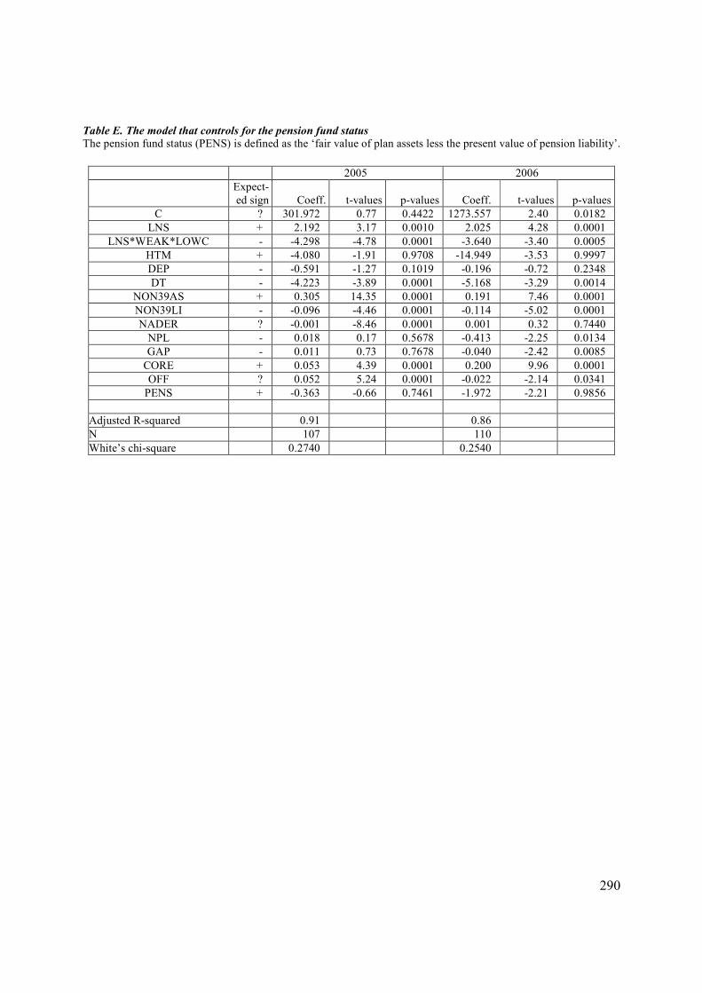
290

Table E. The model that controls for the pension fund status The pension fund status (PENS) is defined as the ‘fair value of plan assets less the present value of pension liability’.

2005 2006

Expect-


C ? 301.972 0.77 0.4422 1273.557 2.40 0.0182

LNS + 2.192 3.17 0.0010 2.025 4.28 0.0001

LNS*WEAK*LOWC - -4.298 -4.78 0.0001 -3.640 -3.40 0.0005

HTM + -4.080 -1.91 0.9708 -14.949 -3.53 0.9997

DEP - -0.591 -1.27 0.1019 -0.196 -0.72 0.2348

DT - -4.223 -3.89 0.0001 -5.168 -3.29 0.0014

NON39AS + 0.305 14.35 0.0001 0.191 7.46 0.0001

NON39LI - -0.096 -4.46 0.0001 -0.114 -5.02 0.0001

NADER ? -0.001 -8.46 0.0001 0.001 0.32 0.7440

NPL - 0.018 0.17 0.5678 -0.413 -2.25 0.0134

GAP - 0.011 0.73 0.7678 -0.040 -2.42 0.0085

CORE + 0.053 4.39 0.0001 0.200 9.96 0.0001

OFF ? 0.052 5.24 0.0001 -0.022 -2.14 0.0341

PENS + -0.363 -0.66 0.7461 -1.972 -2.21 0.9856


N 107 110


291

Section 2: Tables of the alternative specification models from the value relevance test – derivatives’ fair

values

Table A. The March model The dependent variable is the market value of equity (March prices).

2005 2006

Expect-


C ? 742.861 1.82 0.0707 1076.790 2.03 0.0445

BV + 2.193 16.76 0.0001 1.632 10.01 0.0001

NOI + 1.073 2.61 0.0052 1.856 4.03 0.0001

NSI + 1.806 6.98 0.0001 2.594 5.71 0.0001

NTDER + 2.462 6.12 0.0001 0.206 0.39 0.3470

NTDER*WEAK*VARIN - -1.051 -3.70 0.0002 -0.951 -1.86 0.0328

NHDER + 3.066 7.38 0.0001 0.535 0.76 0.2239

NHDER*WEAK*VARIN - 0.602 1.50 0.9317 0.239 0.21 0.5868

NADER ? 0.001 2.41 0.0177 -0.001 -3.41 0.0010

NPL - -0.563 -4.83 0.0001 -1.085 -4.51 0.0001

GAP - -0.015 -1.31 0.0967 -0.002 -0.13 0.4471

CORE + -0.121 -7.93 0.9999 -0.016 -0.54 0.7080

OFF ? -0.026 -2.13 0.0353 -0.040 -2.83 0.0057


N 105 107


Table B. The growth model The growth variable (LNS_5YR_CH) is the five years change in net loans.

2005 2006


C ? 406.461 0.91 0.3601 998.064 1.85 0.0669

BV + 2.117 12.41 0.0001 1.639 8.95 0.0001

NOI + 0.897 1.82 0.0355 1.756 3.78 0.0002

NSI + 1.287 4.58 0.0001 2.499 5.54 0.0001

NTDER + 1.952 4.22 0.0001 0.222 0.39 0.3481

NTDER*WEAK*VARIN - -1.120 -3.62 0.0003 -0.931 -1.75 0.0414

NHDER + 2.763 7.45 0.0001 0.844 1.44 0.0763

NHDER*WEAK*VARIN - 0.394 1.03 0.8478 0.990 0.98 0.8369

NADER ? 0.001 1.46 0.1471 -0.001 -2.86 0.0051

NPL - -0.667 -5.14 0.0001 -0.978 -4.20 0.0001

GAP - 0.001 0.07 0.5313 -0.016 -1.07 0.1435

CORE + -0.074 -4.39 0.9999 0.003 0.10 0.4578

OFF ? -0.037 -2.78 0.0065 -0.048 -3.25 0.0015

LNS_5YR_CH + 0.004 0.40 0.3440 0.001 0.01 0.4922


N 107 109


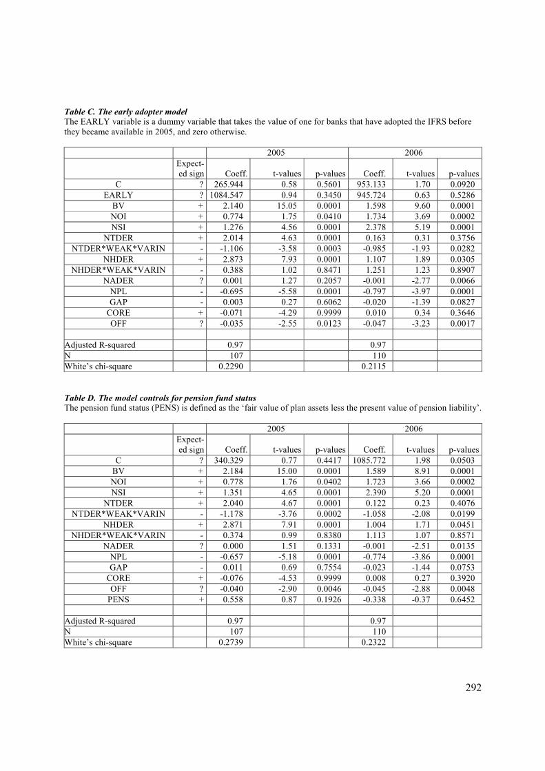
292

Table C. The early adopter model The EARLY variable is a dummy variable that takes the value of one for banks that have adopted the IFRS before they became available in 2005, and zero otherwise.

2005 2006


C ? 265.944 0.58 0.5601 953.133 1.70 0.0920

EARLY ? 1084.547 0.94 0.3450 945.724 0.63 0.5286

BV + 2.140 15.05 0.0001 1.598 9.60 0.0001

NOI + 0.774 1.75 0.0410 1.734 3.69 0.0002

NSI + 1.276 4.56 0.0001 2.378 5.19 0.0001

NTDER + 2.014 4.63 0.0001 0.163 0.31 0.3756

NTDER*WEAK*VARIN - -1.106 -3.58 0.0003 -0.985 -1.93 0.0282

NHDER + 2.873 7.93 0.0001 1.107 1.89 0.0305

NHDER*WEAK*VARIN - 0.388 1.02 0.8471 1.251 1.23 0.8907

NADER ? 0.001 1.27 0.2057 -0.001 -2.77 0.0066

NPL - -0.695 -5.58 0.0001 -0.797 -3.97 0.0001

GAP - 0.003 0.27 0.6062 -0.020 -1.39 0.0827

CORE + -0.071 -4.29 0.9999 0.010 0.34 0.3646

OFF ? -0.035 -2.55 0.0123 -0.047 -3.23 0.0017


N 107 110


Table D. The model controls for pension fund status The pension fund status (PENS) is defined as the ‘fair value of plan assets less the present value of pension liability’.

2005 2006


C ? 340.329 0.77 0.4417 1085.772 1.98 0.0503

BV + 2.184 15.00 0.0001 1.589 8.91 0.0001

NOI + 0.778 1.76 0.0402 1.723 3.66 0.0002

NSI + 1.351 4.65 0.0001 2.390 5.20 0.0001

NTDER + 2.040 4.67 0.0001 0.122 0.23 0.4076

NTDER*WEAK*VARIN - -1.178 -3.76 0.0002 -1.058 -2.08 0.0199

NHDER + 2.871 7.91 0.0001 1.004 1.71 0.0451

NHDER*WEAK*VARIN - 0.374 0.99 0.8380 1.113 1.07 0.8571

NADER ? 0.000 1.51 0.1331 -0.001 -2.51 0.0135

NPL - -0.657 -5.18 0.0001 -0.774 -3.86 0.0001

GAP - 0.011 0.69 0.7554 -0.023 -1.44 0.0753

CORE + -0.076 -4.53 0.9999 0.008 0.27 0.3920

OFF ? -0.040 -2.90 0.0046 -0.045 -2.88 0.0048

PENS + 0.558 0.87 0.1926 -0.338 -0.37 0.6452


N 107 110


293

Table E. The model that disaggregates the notional amounts of derivatives in hedging and trading NATDER is the notional amounts of trading derivatives and NAHDER is the notional amounts of hedging derivatives.

2005 2006

Expect-


C ? 64.0245 0.25 0.7957 649.100 2.26 0.0263

BV + 1.779 12.22 0.0001 1.496 13.30 0.0001

NOI + 0.240 0.84 0.2012 0.530 1.61 0.0554

NSI + 0.865 3.98 0.0001 0.556 1.29 0.1005

NTDER + 1.523 5.09 0.0001 1.725 5.29 0.0001

NTDER*WEAK*VARIN - -0.924 -3.04 0.0017 0.079 0.16 0.5650

NHDER + 1.905 6.18 0.0001 1.507 2.86 0.0027

NHDER*WEAK*VARIN - -0.640 -1.19 0.1175 -0.350 -0.28 0.3883

NATDER ? -0.001 -2.74 0.0078 -0.001 -3.76 0.0001

NAHDER ? 0.001 0.28 0.7764 -0.004 -0.65 0.5144

NPL - -0.471 -4.38 0.0001 -0.433 -3.64 0.0003

GAP - 0.007 0.57 0.7170 0.019 1.66 0.9504

CORE + -0.005 -0.29 0.6169 0.051 2.45 0.0083

OFF ? 0.001 0.07 0.9377 -0.010 -0.98 0.3301


N 83 88


Table F. The balance sheet model Where, FVFAS is the aggregated fair values of the financial assets and FVFLI is the aggregated fair values of the

financial liabilities.

2005 2006


C ? 274.343 0.81 0.4159 395.435 0.92 0.3569

FVFAS + 0.887 6.83 0.0001 1.097 8.53 0.0001

FVFLI - -0.845 -6.32 0.0001 -1.038 -7.92 0.0001

NON39AS + 0.990 7.53 0.0001 1.117 8.99 0.0001

NON39LI - -0.995 -8.11 0.0001 -1.189 -9.98 0.0001

NTDER + -0.427 -1.11 0.8664 -0.968 -2.45 0.9920

NTDER*WEAK*VARIN - -1.435 -5.35 0.0001 -1.868 -4.64 0.0001

NHDER + 2.277 8.44 0.0001 2.897 5.64 0.0001

NHDER*WEAK*VARIN - -1.899 -6.86 0.0001 -1.654 -2.09 0.0193

NADER ? -0.001 -6.64 0.0001 -0.001 -7.26 0.0001

NPL - -0.567 -5.15 0.0001 -0.600 -3.64 0.0004

GAP - 0.002 0.22 0.5876 -0.038 -3.19 0.0019

CORE + 0.031 2.16 0.0164 0.059 2.21 0.0144

OFF ? 0.047 4.53 0.0001 -0.001 -0.05 0.9550


N 107 110


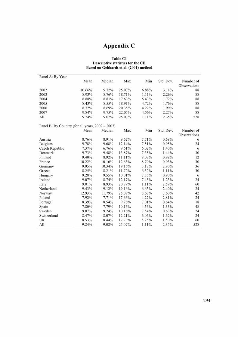
294

Appendix C

Table C1

Descriptive statistics for the CE

Based on Gebhardt et al. (2001) method


Observations 2002 10.66% 9.72% 25.07% 6.88% 3.11% 88 2003 8.93% 8.76% 18.71% 1.11% 2.26% 88 2004 8.88% 8.81% 17.63% 5.43% 1.72% 88 2005 8.43% 8.55% 18.91% 4.72% 1.76% 88

2006 8.72% 8.69% 20.35% 4.22% 1.99% 88 2007 9.84% 9.75% 22.05% 4.56% 2.27% 88

All 9.24% 9.02% 25.07% 1.11% 2.35% 528

Panel B: By Country (for all years, 2002 – 2007) Mean Median Max Min Std. Dev. Number of

Observations Austria 8.76% 8.91% 9.62% 7.71% 0.68% 6 Belgium 9.78% 9.68% 12.14% 7.51% 0.95% 24

Czech Republic 7.37% 6.76% 9.61% 6.02% 1.40% 6 Denmark 9.73% 9.48% 13.87% 7.35% 1.44% 30

Finland 9.40% 8.92% 11.11% 8.07% 0.98% 12 France 10.22% 10.16% 12.63% 8.70% 0.93% 30

Germany 9.95% 10.34% 19.16% 5.17% 2.90% 36 Greece 8.25% 8.21% 11.72% 6.32% 1.11% 30

Hungary 9.28% 9.55% 10.01% 7.55% 0.90% 6 Ireland 9.07% 8.74% 12.17% 7.45% 1.23% 24 Italy 9.01% 8.93% 20.79% 1.11% 2.59% 60

Netherland 9.43% 9.12% 19.16% 6.63% 2.40% 24 Norway 12.93% 11.79% 25.07% 8.60% 3.60% 42 Poland 7.92% 7.71% 17.66% 4.22% 2.81% 24 Portugal 8.39% 8.54% 9.26% 7.01% 0.64% 18

Spain 7.80% 7.79% 10.16% 4.56% 1.33% 48 Sweden 9.07% 9.24% 10.16% 7.54% 0.63% 24

Switzerland 8.47% 8.07% 12.21% 6.05% 1.62% 24 UK 8.53% 8.44% 12.73% 5.25% 1.50% 60 All 9.24% 9.02% 25.07% 1.11% 2.35% 528

295

Table C2


Based on Claus & Thomas (2001) method


Observations 2002 11.71% 11.06% 29.82% 4.48% 4.01% 88

2003 10.02% 10.05% 20.14% 4.49% 2.31% 87 2004 9.98% 10.25% 21.25% 0.74% 2.70% 87 2005 9.04% 9.39% 12.87% 3.55% 1.86% 87 2006 9.24% 9.47% 13.96% 4.15% 1.98% 88 2007 10.54% 10.60% 20.59% 4.00% 2.65% 88

All 10.09% 10.04% 29.82% 0.74% 2.81% 525


Observations Austria 10.60% 10.31% 13.33% 9.30% 1.44% 6

Belgium 9.58% 10.67% 13.12% 3.55% 2.93% 24 Czech Republic 9.25% 9.37% 10.74% 7.50% 1.12% 6 Denmark 9.44% 9.35% 16.42% 6.35% 2.10% 30

Finland 9.81% 9.05% 13.03% 7.28% 1.98% 12 France 10.95% 10.32% 19.00% 7.47% 2.48% 30

Germany 11.21% 9.88% 29.82% 5.40% 5.12% 36 Greece 11.71% 11.77% 14.89% 6.62% 1.83% 30

Hungary 11.02% 11.07% 11.95% 9.93% 0.81% 6 Ireland 11.17% 10.88% 15.29% 8.66% 1.51% 24

Italy 9.85% 10.00% 26.83% 0.74% 3.60% 58 Netherland 10.76% 10.44% 14.55% 4.48% 2.18% 23 Norway 7.99% 7.69% 13.00% 4.64% 2.12% 42

Poland 11.11% 9.14% 21.97% 6.99% 4.41% 24 Portugal 9.80% 9.93% 12.06% 7.10% 1.26% 18 Spain 9.59% 9.93% 14.04% 5.54% 1.82% 48 Sweden 9.75% 9.68% 11.00% 8.50% 0.72% 24

Switzerland 8.45% 7.92% 14.39% 5.06% 2.42% 24 UK 10.60% 10.62% 15.05% 7.38% 1.77% 60

All 10.09% 10.04% 29.82% 0.74% 2.81% 525

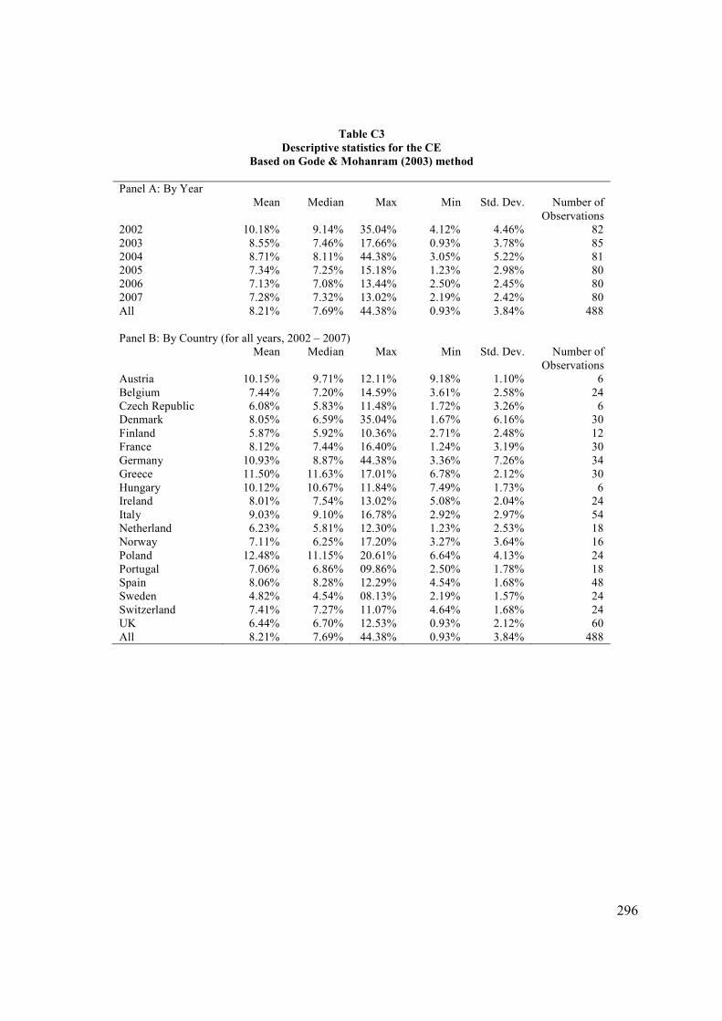
296

Table C3


Based on Gode & Mohanram (2003) method


Observations 2002 10.18% 9.14% 35.04% 4.12% 4.46% 82

2003 8.55% 7.46% 17.66% 0.93% 3.78% 85 2004 8.71% 8.11% 44.38% 3.05% 5.22% 81 2005 7.34% 7.25% 15.18% 1.23% 2.98% 80 2006 7.13% 7.08% 13.44% 2.50% 2.45% 80 2007 7.28% 7.32% 13.02% 2.19% 2.42% 80

All 8.21% 7.69% 44.38% 0.93% 3.84% 488




Finland 5.87% 5.92% 10.36% 2.71% 2.48% 12 France 8.12% 7.44% 16.40% 1.24% 3.19% 30

Germany 10.93% 8.87% 44.38% 3.36% 7.26% 34 Greece 11.50% 11.63% 17.01% 6.78% 2.12% 30

Hungary 10.12% 10.67% 11.84% 7.49% 1.73% 6 Ireland 8.01% 7.54% 13.02% 5.08% 2.04% 24



Switzerland 7.41% 7.27% 11.07% 4.64% 1.68% 24 UK 6.44% 6.70% 12.53% 0.93% 2.12% 60

All 8.21% 7.69% 44.38% 0.93% 3.84% 488

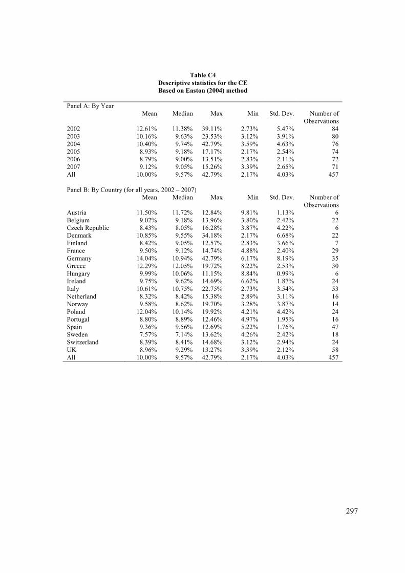
297

Table C4


Based on Easton (2004) method


Observations 2002 12.61% 11.38% 39.11% 2.73% 5.47% 84

2003 10.16% 9.63% 23.53% 3.12% 3.91% 80 2004 10.40% 9.74% 42.79% 3.59% 4.63% 76 2005 8.93% 9.18% 17.17% 2.17% 2.54% 74 2006 8.79% 9.00% 13.51% 2.83% 2.11% 72 2007 9.12% 9.05% 15.26% 3.39% 2.65% 71

All 10.00% 9.57% 42.79% 2.17% 4.03% 457




Finland 8.42% 9.05% 12.57% 2.83% 3.66% 7 France 9.50% 9.12% 14.74% 4.88% 2.40% 29

Germany 14.04% 10.94% 42.79% 6.17% 8.19% 35 Greece 12.29% 12.05% 19.72% 8.22% 2.53% 30

Hungary 9.99% 10.06% 11.15% 8.84% 0.99% 6 Ireland 9.75% 9.62% 14.69% 6.62% 1.87% 24



Switzerland 8.39% 8.41% 14.68% 3.12% 2.94% 24 UK 8.96% 9.29% 13.27% 3.39% 2.12% 58

All 10.00% 9.57% 42.79% 2.17% 4.03% 457

29

8

Appendix D

Robustness tests of the additional analysis on the economic consequences test

Table D1


Using alternative control variables to some variables used in the model of Table 9.10

r G

LS

r C

T

r O

J

r PE

G

r A

VG

Var

iable

s C

oef

f.

t-val

ue

C

oef

f.

t-val

ue

C

oef

f.

t-val

ue

C

oef

f.

t-val

ue

C

oef

f.

t-val

ue

Inte

rcep

t 0

.06

07

4.8

259

***

0.0

453

1.9

779

***

0.0

461

1.6

624

***

0.0

028

0.0

941

***

0.0

624

3.6

003

***

P

OS

T

-0.0

11

9

-2.6

31

8***

-0

.02

60

-3.1

64

9***

-0.0

14

9

-1.5

19

7***

-0.0

09

3

-0.9

63

7***

-0.0

19

4

-3.1

234

***

M

AN

D

-0.0

07

0

-0.8

32

1***

0.0

115

0.7

479

***

-0.0

04

6

-0.2

52

8***

0.0

419

1.9

715

***

-0.0

03

3

-0.2

881

***

L

OW

F

-0.0

07

0

-0.9

34

0***

-0

.00

31

-0.2

26

1***

0.0

880

5.3

908

***

0.0

461

2.8

591

***

0.0

294

2.8

228

***

P

OS

T*M

AN

D

0.0

140

3.0

148

***

0.0

217

2.5

685

***

0.0

056

0.5

591

***

0.0

017

0.1

767

***

0.0

143

2.2

413

***

P

OS

T*L

OW

F

0.0

080

1.2

218

***

0.0

161

1.3

475

***

-0.0

21

8

-1.5

43

4***

-0.0

09

4

-0.6

81

8***

0.0

005

0.0

596

***

M

AN

D*

LO

WF

0

.01

16

1.5

248

***

0.0

025

0.1

855

***

-0.0

79

5

-4.7

98

9***

-0.0

43

5

-2.6

62

4***

-0.0

25

2

-2.3

990

***

P

OS

T*M

AN

D*

LO

WF

-0

.02

12

-3.0

87

8***

-0

.03

23

-2.5

73

3***

0.0

172

1.1

441

***

0.0

041

0.2

755

***

-0.0

11

5

-1.2

123

***

C

AR

-0

.04

00

-1.6

45

9***

0.0

406

0.9

164

***

-0.0

06

6

-0.1

27

4***

-0.0

51

8

-0.9

74

3***

-0.0

15

4

-0.4

617

***

L

D

-0.0

01

3

-2.2

68

9***

-0

.00

43

-3.9

21

0***

-0.0

04

5

-3.5

09

9***

-0.0

05

7

-3.6

76

4***

-0.0

03

6

-4.3

349

***

R

VA

R

0.0

885

3.9

805

***

0.0

711

1.7

533

***

0.0

781

1.6

142

***

0.1

909

3.8

694

***

0.1

036

3.3

766

***

V

AR

CO

EF

-0

.00

01

-1.4

41

6***

-0

.00

01

-2.0

50

9***

0.0

005

6.5

155

***

0.0

009

9.3

215

***

0.0

002

4.3

014

***

B

M

0.0

169

16

.661

8***

-0

.00

01

-0.0

54

9***

0.0

215

2.7

569

***

0.0

325

4.1

202

***

0.0

083

5.9

559

***

L

OG

(MV

E)

-0.0

00

5

-0.7

92

7***

0.0

005

0.3

992

***

-0.0

00

2

-0.1

53

5***

0.0

008

0.5

233

***

-0.0

00

5

-0.5

581

***

L

EV

0

.00

05

1.9

581

***

0.0

010

1.8

886

***

0.0

007

1.1

394

***

0.0

013

1.9

179

***

0.0

008

1.9

835

***

R

F

0.0

059

8.6

603

***

0.0

086

6.8

925

***

0.0

023

1.5

078

***

0.0

037

2.3

148

***

0.0

056

5.9

534

***

U

SL

IST

0

.00

53

2.3

414

***

0.0

043

1.0

507

***

0.0

012

0.2

440

***

-0.0

02

8

-0.5

68

9***

0.0

034

1.0

864

***

C

ou

ntr

y d

um

mie

s In

clu

ded

In

clu

ded

In

clu

ded

In

clu

ded

In

clu

ded

N

43

0

430

41

4

38

2

43

0

A

dj.

R2

0.6

9

0.3

2

0.5

5

0.5

3

0.5

1

Th

e *** i

ndic

ates

p-v

alu

es <

0.0

1,

** i

ndic

ates

p-v

alu

es <

0.0

5,

and

* i

ndic

ates

p-v

alu

es <

0.1

0.

29

9

Table D2



r G

LS

r C

T

r O

J

r PE

G

r A

VG

Var

iable

s C

oef

f.

t-val

ue

C

oef

f.

t-val

ue

C

oef

f.

t-val

ue

C

oef

f.

t-val

ue

C

oef

f.

t-val

ue

Inte

rcep

t 0

.06

67

5.5

125

***

0.0

846

3.6

191

***

0.0

723

2.2

361

***

0.0

749

2.1

035

***

0.0

815

4.3

984

***

P

OS

T

-0.0

12

1

-2.9

05

0***

-0

.02

34

-2.9

02

5***

-0.0

38

3

-3.5

93

7***

-0.0

51

2

-4.5

48

3***

-0.0

30

9

-4.8

286

***

M

AN

D

0.0

006

0.0

886

***

-0

.00

68

-0.5

05

3***

0.0

086

0.4

812

***

0.0

014

0.0

731

***

-0.0

00

6

-0.0

584

***

L

OW

F

-0.0

02

2

-0.3

40

5***

0.0

037

0.2

992

***

0.0

891

5.3

608

***

0.0

538

3.0

560

***

0.0

349

3.5

022

***

P

OS

T*M

AN

D

0.0

135

3.1

139

***

0.0

194

2.3

020

***

0.0

242

2.1

839

***

0.0

351

2.9

801

***

0.0

231

3.4

605

***

P

OS

T*L

OW

F

0.0

077

1.2

755

***

0.0

122

1.0

405

***

-0.0

07

3

-0.4

72

5***

0.0

126

0.7

696

***

0.0

060

0.6

447

***

M

AN

D*

LO

WF

0

.00

78

1.1

923

***

-0

.00

41

-0.3

23

2***

-0.0

84

0

-4.9

90

7***

-0.0

51

1

-2.8

67

7***

-0.0

32

2

-3.1

913

***

P

OS

T*M

AN

D*

LO

WF

-0

.01

34

-2.0

62

7

-0

.02

60

-2.0

67

8***

0.0

034

0.2

031

***

-0.0

16

5

-0.9

33

1***

-0.0

12

0

-1.2

056

***

L

OG

(CA

R)

-0.0

09

9

-3.0

04

5***

0.0

023

0.3

616

***

-0.0

01

8

-0.2

14

3***

-0.0

10

4

-1.1

15

4***

-0.0

05

1

-1.0

119

***

L

OG

(LD

) -0

.00

35

-2.2

12

8***

-0

.00

72

-2.3

38

8***

-0.0

15

3

-3.7

59

0***

-0.0

11

9

-2.5

96

2***

-0.0

09

7

-3.9

790

***

L

OG

(BE

TA

) 0

.00

52

3.9

313

***

0.0

042

1.6

457

***

-0.0

03

0

-0.8

60

2***

0.0

030

0.8

033

***

0.0

025

1.2

607

***

L

OG

(VA

RE

RN

) 0

.00

22

3.0

792

***

-0

.00

05

-0.3

51

1***

0.0

119

6.1

362

***

0.0

112

5.3

887

***

0.0

061

5.3

532

***

L

OG

(BM

) 0

.03

38

20

.249

4***

0.0

096

2.9

903

***

0.0

193

3.6

191

***

0.0

250

4.3

454

***

0.0

223

8.7

366

***

L

OG

(AS

SE

T)

0.0

005

0.7

558

***

0.0

006

0.4

191

***

0.0

001

0.0

290

***

0.0

012

0.5

509

***

0.0

001

0.1

338

***

L

OG

(LE

V)

0.0

008

1.6

560

***

0.0

014

1.5

230

***

0.0

014

1.1

439

***

0.0

002

0.1

525

***

0.0

010

1.3

690

***

R

F

0.0

039

6.1

913

***

0.0

079

6.3

840

***

0.0

032

1.8

830

***

0.0

047

2.5

052

***

0.0

049

5.0

145

***

U

SL

IST

0

.00

14

0.6

705

***

0.0

006

0.1

401

***

-0.0

03

0

-0.5

28

6***

-0.0

07

9

-1.2

76

2***

-0.0

01

4

-0.4

208

***

C

ou

ntr

y d

um

mie

s In

clu

ded

In

clu

ded

In

clu

ded

In

clu

ded

In

clu

ded

N

44

2

442

42

0

38

8

44

2

A

dj.

R2

0.7

3

0.3

3

0.5

2

0.4

3

0.5

3

Th

e *** i

ndic

ates

p-v

alu

es <

0.0

1,

** i

ndic

ates

p-v

alu

es <

0.0

5,

and

* i

ndic

ates

p-v

alu

es <

0.1

0.

30

0

Table D3



r G

LS

r C

T

r O

J

r PE

G

r A

VG

Var

iable

s C

oef

f.

t-val

ue

C

oef

f.

t-val

ue

C

oef

f.

t-val

ue

C

oef

f.

t-val

ue

C

oef

f.

t-val

ue

Inte

rcep

t 0

.04

39

3.0

583

***

0.0

132

0.5

041

***

0.0

410

1.0

983

***

0.0

450

1.0

810

***

0.0

558

2.5

114

***

P

OS

T

-0.0

17

0

-4.0

33

7***

-0

.02

43

-3.1

56

3***

-0.0

30

0

-2.8

10

9***

-0.0

42

4

-3.8

16

5***

-0.0

32

8

-5.0

330

***

M

AN

D

-0.0

02

5

-0.3

07

5***

0.0

224

1.4

621

***

-0.0

05

9

-0.2

86

6***

0.0

050

0.1

977

***

-0.0

02

4

-0.1

899

***

L

OW

F

-0.0

01

4

-0.2

03

3***

0.0

139

1.0

590

***

0.0

777

4.3

351

***

0.0

280

1.4

843

***

0.0

307

2.7

740

***

P

OS

T*M

AN

D

0.0

162

3.6

339

***

0.0

184

2.2

517

***

0.0

179

1.5

962

***

0.0

278

2.3

593

***

0.0

240

3.4

777

***

P

OS

T*L

OW

F

0.0

116

1.8

484

***

0.0

119

1.0

349

***

-0.0

14

6

-0.9

28

7***

0.0

110

0.6

773

***

0.0

066

0.6

858

***

M

AN

D*

LO

WF

0

.00

91

1.2

790

***

-0

.01

28

-0.9

76

6***

-0.0

72

2

-4.0

21

7***

-0.0

29

2

-1.5

52

1***

-0.0

26

2

-2.3

616

***

P

OS

T*M

AN

D*

LO

WF

-0

.02

28

-3.4

00

1

-0

.02

61

-2.1

31

8***

0.0

122

0.7

254

***

-0.0

10

6

-0.6

00

9***

-0.0

16

0

-1.5

468

***

C

AR

-0

.03

55

-1.4

26

1***

0.0

733

1.6

067

***

0.0

742

1.1

898

***

0.0

117

0.1

742

***

0.0

274

0.7

121

***

L

D

-0.0

01

4

-2.3

94

2***

-0

.00

43

-4.0

71

2***

-0.0

06

6

-4.5

14

7***

-0.0

07

2

-3.7

73

9***

-0.0

04

7

-5.1

688

***

B

ET

A

0.0

082

3.3

888

***

0.0

018

0.4

220

***

-0.0

01

9

-0.3

10

4***

0.0

063

0.9

610

***

0.0

032

0.8

482

***

V

AR

ER

N

0.0

001

1.1

148

***

-0

.00

01

-0.9

14

6***

0.0

004

1.7

799

***

0.0

005

2.2

334

***

0.0

002

1.7

070

***

B

M

0.0

172

18

.606

7***

0.0

002

0.1

440

***

0.0

396

4.9

470

***

0.0

515

6.0

310

***

0.0

094

6.5

729

***

LO

G(A

SS

ET

) 0

.00

02

0.3

547

***

0.0

019

1.3

570

***

-0.0

00

7

-0.3

48

6***

-0.0

00

5

-0.2

34

4***

-0.0

00

3

-0.3

131

***

L

EV

0

.00

07

2.3

732

***

0.0

009

1.8

254

***

0.0

010

1.3

664

***

0.0

011

1.4

335

***

0.0

010

2.2

605

***

R

F

0.0

063

9.7

389

***

0.0

090

7.5

637

***

0.0

035

2.0

437

***

0.0

057

3.0

238

***

0.0

069

6.9

258

***

U

SL

IST

0

.00

25

1.0

880

***

0.0

014

0.3

320

***

0.0

024

0.4

137

***

-0.0

02

5

-0.4

05

3***

0.0

023

0.6

405

***

L

TG

0

.00

31

1.4

460

***

0.0

109

2.7

581

***

-0.0

01

2

-0.2

35

5***

-0.0

14

3

-2.3

95

8***

0.0

018

0.5

566

***

C

ou

ntr

y d

um

mie

s In

clu

ded

In

clu

ded

In

clu

ded

In

clu

ded

In

clu

ded

N

44

4

444

42

2

39

0

44

4

A

dj.

R2

0.7

0

0.3

4

0.5

0

0.4

1

0.4

7

Th

e *** i

ndic

ates

p-v

alu

es <

0.0

1,

** i

ndic

ates

p-v

alu

es <

0.0

5,

and

* i

ndic

ates

p-v

alu

es <

0.1

0.

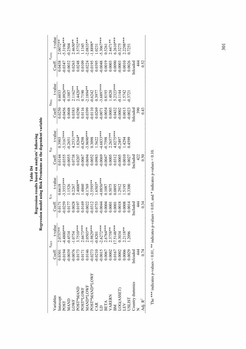
30

1

Table D4



r G

LS

r C

T

r O

J

r PE

G

r A

VG

Var

iable

s C

oef

f.

t-val

ue

C

oef

f.

t-val

ue

C

oef

f.

t-val

ue

C

oef

f.

t-val

ue

C

oef

f.

t-val

ue

Inte

rcep

t 0

.03

01

2.0

757

***

0

.01

71

0.6

618

***

0.0

144

0.3

903

***

0.0

250

0.6

033

***

0.0

438

2.0

072

***

P

OS

T

-0.0

19

4

-4.4

80

0***

-0

.02

59

-3.3

55

3***

-0

.03

55

-3.3

16

7***

-0.0

45

6

-4.0

92

6***

-0.0

34

7

-5.3

196

***

M

AN

D

-0.0

03

9

-0.4

53

4***

0

.01

77

1.1

526

***

-0

.00

55

-0.2

65

1***

0.0

048

0.1

887

***

-0.0

03

2

-0.2

504

***

L

OW

F

-0.0

07

6

-1.0

75

4***

0

.00

28

0.2

267

***

0.0

738

4.2

531

***

0.0

383

2.1

162

***

0.0

263

2.4

650

***

P

OS

T*M

AN

D

0.0

173

3.7

510

***

0

.01

97

2.4

008

***

0.0

207

1.8

264

***

0.0

290

2.4

420

***

0.0

248

3.5

752

***

P

OS

T*L

OW

F

0.0

171

2.6

673

***

0

.01

69

1.4

860

***

-0

.00

67

-0.4

29

8***

0.0

116

0.7

190

***

0.0

109

1.1

345

***

M

AN

D*

LO

WF

0

.01

46

2.0

503

***

-0

.00

22

-0.1

76

9***

-0

.06

94

-3.9

69

0***

-0.0

39

9

-2.1

89

4***

-0.0

22

4

-2.0

835

***

P

OS

T*M

AN

D*

LO

WF

-0

.02

73

-3.9

82

9***

-0

.03

12

-2.5

59

5***

0.0

052

0.3

098

***

-0.0

11

0

-0.6

24

2***

-0.0

19

5

-1.8

898

***

C

AR

-0

.02

10

-0.8

20

1***

0

.07

53

1.6

503

***

0.0

983

1.5

622

***

0.0

269

0.3

977

***

0.0

395

1.0

231

***

L

D

-0.0

01

5

-2.6

27

2***

-0

.00

44

-4.0

85

6***

-0

.00

69

-4.6

83

3***

-0.0

07

1

-3.6

89

7***

-0.0

04

8

-5.3

067

***

B

ET

A

0.0

067

2.6

764

***

0

.00

04

0.1

087

***

-0

.00

47

-0.7

59

8***

0.0

054

0.8

193

***

0.0

019

0.5

261

***

V

AR

ER

N

0.0

002

2.3

758

***

0

.00

01

0.5

075

***

0.0

005

2.2

657

***

0.0

003

1.4

820

***

0.0

003

2.4

471

***

B

M

0.0

167

17

.514

8***

0

.00

01

0.0

895

***

0.0

312

4.0

275

***

0.0

432

5.2

323

***

0.0

090

6.2

610

***

L

OG

(AS

SE

T)

0.0

002

0.3

034

***

0

.00

18

1.2

912

***

-0

.00

05

-0.2

49

7***

-0.0

00

2

-0.1

14

4***

-0.0

00

3

-0.3

275

***

L

EV

0

.00

06

2.2

118

***

0

.00

08

1.5

195

***

0.0

010

1.4

294

***

0.0

013

1.5

742

***

0.0

010

2.2

298

***

U

SL

IST

0

.00

29

1.2

096

***

0

.00

14

0.3

300

***

0.0

027

0.4

599

***

-0.0

02

3

-0.3

72

1***

0.0

026

0.7

251

***

C

ou

ntr

y d

um

mie

s In

lcu

ded

In

clu

ded

In

clu

ded

In

lcu

ded

In

lcu

ded

N

44

4

44

4

422

39

0

44

4

A

dj.

R2

0.7

4

0.3

4

0.5

0

0.4

3

0.5

2

Th

e *** i

ndic

ates

p-v

alu

es <

0.0

1,

** i

ndic

ates

p-v

alu

es <

0.0

5,

and

* i

ndic

ates

p-v

alu

es <

0.1

0.

30

2

Table D5

Regression results based on accounting classification

Using alternative control variables to some variables used in the model of Table 9.11

r GL

S

r C

T

r O

J

r PE

G

r A

VG

Var

iable

s C

oef

f.

t-val

ue

C

oef

f.

t-val

ue

C

oef

f.

t-val

ue

C

oef

f.

t-val

ue

C

oef

f.

t-val

ue

Inte

rcep

t 0.0525

4.3613***

0.0305

1.4084***

0.1009

3.8060***

0.0242

0.8512***

0.0739

4.5007***

PO

ST

-0.0013

-0.5870***

-0.0081

-2.0017***

-0.0071

-1.4096***

-0.0094

-1.8095***

-0.0065

-2.1273***

MA

ND

-0.0038

-0.4674***

0.0107

0.7181***

-0.0273

-1.5310***

0.0324

1.5603***

-0.0110

-0.9750***

PO

ST

*C

ON

T

-0.0078

-1.9229***

-0.0117

-1.5928***

-0.0148

-1.6693***

-0.0023

-0.2694***

-0.0121

-2.1812***

PO

ST

*M

AN

D*C

ON

T

0.0042

1.1289***

0.0057

0.8488***

0.0107

1.3458***

0.0027

0.3499***

0.0074

1.4723***

CA

R

-0.0356

-1.4138***

0.0441

0.9715***

-0.0189

-0.3496***

-0.0540

-1.0042***

-0.0175

-0.5110***

LD

-0.0014

-2.2801***

-0.0045

-4.0465***

-0.0047

-3.5537***

-0.0063

-3.9980***

-0.0037

-4.4524***

RV

AR

0.0709

3.2337***

0.0601

1.5196***

0.0558

1.1730***

0.1770

3.7407***

0.0867

2.9011***

VA

RC

OE

F

-0.0001

-1.4206***

-0.0001

-1.9749***

0.0006

6.8683***

0.0009

9.7105***

0.0002

4.5763***

BM

0.0172

16.547***

0.0003

0.1814***

0.0170

2.1821***

0.0316

4.1126***

0.0080

5.6820***

LO

G(M

VE

) -0.0001

-0.0660***

0.0021

1.9140***

-0.0036

-2.5046***

-0.0004

-0.2935***

-0.0009

-1.1364***

LE

V

0.0008

2.6572***

0.0014

2.6531***

0.0008

1.2969***

0.0015

2.3087***

0.0010

2.5633***

RF

0.0061

8.7376***

0.0086

6.7785***

0.0032

1.9864***

0.0042

2.6738***

0.0059

6.1414***

US

LIS

T

0.0054

2.3033***

0.0044

1.0506***

0.0060

1.1806***

-0.0001

-0.0141***

0.0050

1.5739***

Co

un

try d

um

mie

s In

clu

ded

In

clu

ded

In

clu

ded

In

clu

ded

In

clu

ded

N

43

0

430

41

4

38

2

43

0

A

dj.

R2

0.6

7

0.2

9

0.5

2

0.5

2

0.4

9

T

he

*** i

ndic

ates

p-v

alu

es <

0.0

1,

** i

ndic

ates

p-v

alu

es <

0.0

5,

and

* i

ndic

ates

p-v

alu

es <

0.1

0.

30

3

Table D6



r G

LS

r C

T

r O

J

r PE

G

r A

VG

Var

iable

s C

oef

f.

t-val

ue

C

oef

f.

t-val

ue

C

oef

f.

t-val

ue

C

oef

f.

t-val

ue

C

oef

f.

t-val

ue

Inte

rcep

t 0.0683

5.9952***

0.0766

3.4501***

0.1323

4.2068***

0.1167

3.4289***

0.1009

5.6914***

PO

ST

0.0003

0.1650***

-0.0081

-2.1562***

-0.0107

-1.9460***

-0.0146

-2.3947***

-0.0077

-2.5810***

MA

ND

0.0048

0.7430***

-0.0089

-0.7018***

-0.0219

-1.2711***

-0.0172

-0.9052***

-0.0118

-1.1560***

PO

ST

*C

ON

T

-0.0083

-2.3312***

-0.0101

-1.4532***

-0.0295

-3.0665***

-0.0295

-2.8914***

-0.0199

-3.5694***

PO

ST

*M

AN

D*C

ON

T

0.0072

2.1649***

0.0071

1.1033***

0.0253

2.8837***

0.0279

3.0581***

0.0170

3.2709***

LO

G(C

AR

) -0.0094

-2.8521***

0.0017

0.2670***

-0.0059

-0.6798***

-0.0138

-1.4533***

-0.0067

-1.3145***

LO

G(L

D)

-0.0036

-2.3130***

-0.0068

-2.1931***

-0.0182

-4.3527***

-0.0141

-3.0617***

-0.0108

-4.3731***

LO

G(B

ET

A)

0.0045

3.6440***

0.0057

2.3586***

-0.0029

-0.8846***

0.0038

1.0756***

0.0028

1.4607***

LO

G(V

AR

ER

N)

0.0022

3.0070***

-0.0005

-0.4017***

0.0107

5.3386***

0.0100

4.7728***

0.0056

4.8056***

LO

G(B

M)

0.0345

20.728***

0.0112

3.4526***

0.0213

3.9613***

0.0273

4.7963***

0.0232

8.9531***

LO

G(A

SS

ET

) 0.0002

0.3916***

0.0016

1.2819***

-0.0032

-1.7460***

-0.0012

-0.6248***

-0.0008

-0.7841***

LO

G(L

EV

) 0.0008

1.8110***

0.0014

1.5082***

0.0021

1.6160***

0.0006

0.4987***

0.0013

1.7174***

RF

0.0039

6.1291***

0.0077

6.1659***

0.0032

1.8380***

0.0045

2.3737***

0.0049

4.8661***

US

LIS

T

0.0017

0.7860***

0.0002

0.0511***

0.0026

0.4423***

-0.0036

-0.5874***

0.0004

0.1414***

Co

un

try d

um

mie

s In

clu

ded

In

clu

ded

In

clu

ded

In

clu

ded

In

clu

ded

N

44

2

442

42

0

38

8

44

2

A

dj.

R2

0.7

2

0.3

1

0.4

8

0.4

1

0.5

0

T

he

*** i

nd

icat

es p

-val

ues

< 0

.01

, ** i

ndic

ates

p-v

alu

es <

0.0

5,

and

* i

ndic

ates

p-v

alu

es <

0.1

0.

30

4

Table D7



r G

LS

r C

T

r O

J

r PE

G

r A

VG

Var

iable

s C

oef

f.

t-val

ue

C

oef

f.

t-val

ue

C

oef

f.

t-val

ue

C

oef

f.

t-val

ue

C

oef

f.

t-val

ue

Inte

rcep

t 0.0421

3.1715***

0.0059

0.2462***

0.0992

2.8717***

0.0626

1.6293***

0.0715

3.5016***

PO

ST

-0.0034

-1.6720***

-0.0097

-2.5771***

-0.0118

-2.1101***

-0.0169

-2.7459***

-0.0111

-3.4838***

MA

ND

0.0021

0.2683***

0.0189

1.2901***

-0.0341

-1.7003***

-0.0029

-0.1192***

-0.0114

-0.9237***

PO

ST

*C

ON

T

-0.0078

-2.0440***

-0.0094

-1.3535***

-0.0224

-2.2856***

-0.0195

-1.8854***

-0.0180

-3.0400***

PO

ST

*M

AN

D*C

ON

T

0.0052

1.4883***

0.0051

0.8017***

0.0223

2.5441***

0.0235

2.6071***

0.0156

2.8870***

CA

R

-0.0291

-1.1448***

0.0812

1.7556***

0.0530

0.8338***

0.0079

0.1187***

0.0260

0.6643***

LD

-0.0014

-2.4075***

-0.0046

-4.2413***

-0.0068

-4.6136***

-0.0076

-4.0139***

-0.0049

-5.3154***

BE

TA

0.0071

3.0695***

0.0028

0.6749***

-0.0065

-1.0999***

0.0052

0.8526***

0.0014

0.4020***

VA

RE

RN

0.0001

1.0171***

-0.0001

-0.6302***

0.0006

2.7627***

0.0006

2.6612***

0.0003

2.3805***

BM

0.0173

18.2277***

0.0001

0.0635***

0.0417

5.2313***

0.0535

6.4020***

0.0093

6.4205***

LO

G(A

SS

ET

) 0.0001

0.1472***

0.0026

2.1044***

-0.0029

-1.5451***

-0.0011

-0.5868***

-0.0008

-0.7510***

LE

V

0.0008

2.7758***

0.0013

2.3877***

0.0011

1.4961***

0.0013

1.6082***

0.0012

2.6697***

RF

0.0063

9.5282***

0.0090

7.5066***

0.0039

2.2255***

0.0056

3.0230***

0.0071

6.9781***

US

LIS

T

0.0030

1.3058***

0.0019

0.4526***

0.0069

1.1707***

-0.0006

-0.1023***

0.0041

1.1410***

LT

G

0.0035

1.6406***

0.0099

2.5515***

-0.0082

-1.5395***

-0.0174

-3.0647***

-0.0006

-0.2081***

Co

un

try d

um

mie

s In

clu

ded

In

clu

ded

In

clu

ded

In

clu

ded

In

clu

ded

N

44

2

442

42

0

38

8

44

2

A

dj.

R2

0.7

2

0.3

1

0.4

8

0.4

1

0.5

0

T

he

*** i

ndic

ates

p-v

alu

es <

0.0

1,

** i

ndic

ates

p-v

alu

es <

0.0

5,

and

* i

ndic

ates

p-v

alu

es <

0.1

0.

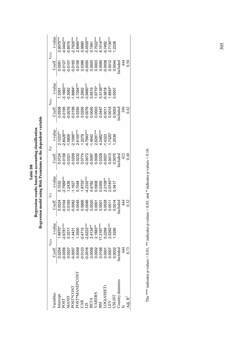
30

5

Table D8



r G

LS

r C

T

r O

J

r PE

G

r A

VG

Var

iable

s C

oef

f.

t-val

ue

C

oef

f.

t-val

ue

C

oef

f.

t-val

ue

C

oef

f.

t-val

ue

C

oef

f.

t-val

ue

Inte

rcep

t 0.0254

1.8970***

0.0024

0.1032***

0.0724

2.1223***

0.0508

1.3351***

0.0581

2.9075***

PO

ST

-0.0056

-2.6781***

-0.0104

-2.7989***

-0.0158

-2.8428***

-0.0195

-3.1660***

-0.0127

-4.0442***

MA

ND

0.0027

0.3317***

0.0183

1.2436***

-0.0321

-1.5809***

-0.0076

-0.3082***

-0.0107

-0.8574***

PO

ST

*C

ON

T

-0.0057

-1.4431***

-0.0082

-1.1827***

-0.0209

-2.1095***

-0.0199

-1.8984***

-0.0165

-2.7925***

PO

ST

*M

AN

D*C

ON

T

0.0049

1.3500***

0.0045

0.7048***

0.0232

2.6105***

0.0250

2.7294***

0.0156

2.8585***

CA

R

-0.0123

-0.4715***

0.0866

1.8755***

0.0774

1.2079***

0.0200

0.2952***

0.0386

0.9880***

LD

-0.0016

-2.6222***

-0.0046

-4.2332***

-0.0072

-4.7993***

-0.0076

-3.9480***

-0.0050

-5.4559***

BE

TA

0.0058

2.4124***

0.0020

0.4782***

-0.0087

-1.4642***

0.0040

0.6519***

0.0005

0.1561***

VA

RE

RN

0.0002

2.1883***

0.0001

0.5908***

0.0006

2.6281***

0.0003

1.6770***

0.0003

2.7022***

BM

0.0168

17.2187***

0.0001

0.0300***

0.0328

4.2482***

0.0447

5.5139***

0.0090

6.1514***

LO

G(A

SS

ET

) 0.0001

0.2269***

0.0028

2.2109***

-0.0027

-1.4323***

-0.0011

-0.5818***

-0.0008

-0.7492***

LE

V

0.0007

2.5282***

0.0011

2.0745***

0.0013

1.7320***

0.0015

1.8597***

0.0012

2.7130***

US

LIS

T

0.0032

1.3295***

0.0014

0.3417***

0.0075

1.2539***

0.0003

0.0557***

0.0044

1.2228***

Co

un

try d

um

mie

s In

clu

ded

In

clu

ded

In

clu

ded

In

clu

ded

In

clu

ded

N

44

4

444

42

2

39

0

44

4

A

dj.

R2

0.7

3

0.3

2

0.4

8

0.4

2

0.5

0

T

he

*** i

ndic

ates

p-v

alu

es <

0.0

1,

** i

ndic

ates

p-v

alu

es <

0.0

5,

and

* i

ndic

ates

p-v

alu

es <

0.1

0.

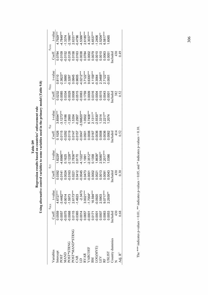
30

6

Table D9


ent rule

Using alternative control variables to some variables used in the primary model (Table 9.8)

r GL

S

r C

T

r O

J

r PE

G

r A

VG

Var

iable

s C

oef

f.

t-val

ue

C

oef

f.

t-val

ue

C

oef

f.

t-val

ue

C

oef

f.

t-val

ue

C

oef

f.

t-val

ue

Inte

rcep

t 0.0559

4.6727***

0.0392

1.8229***

0.1026

3.8594***

0.0232

0.8110***

0.0784

4.7929***

PO

ST

-0.0057

-3.4482***

-0.0141

-4.6986***

-0.0115

-3.1273***

-0.0085

-2.3823***

-0.0109

-4.7849***

MA

ND

-0.0075

-0.9014***

0.0024

0.1625***

-0.0292

-1.6186***

0.0334

1.5880***

-0.0152

-1.3374***

PO

ST

*S

TR

NG

-0.0068

-1.5973***

-0.0163

-2.1228***

-0.0119

-1.2900***

-0.0029

-0.3287***

-0.0128

-2.1990***

PO

ST

*M

AN

D*S

TR

NG

0.0115

2.6173***

0.0221

2.7836***

0.0147

1.5354***

0.0008

0.0845***

0.0158

2.6331***

CA

R

-0.0365

-1.4623***

0.0412

0.9170***

-0.0157

-0.2907***

-0.0515

-0.9605***

-0.0163

-0.4796***

LD

-0.0014

-2.3473

-0.0045

-4.1322***

-0.0047 -3.59820***

-0.0063

-4.0212***

-0.0038

-4.5366***

RV

AR

0.0657

3.0021***

0.0473

1.1991***

0.0501

1.0502***

0.1759

3.7122***

0.0784

2.6185***

VA

RC

OE

F

-0.0001

-1.7004***

-0.0001

-2.3512***

0.0006

6.7408***

0.0009

9.6300***

0.0002

4.3037***

BM

0.0171

16.594***

0.0002

0.1358***

0.0167

2.1311***

0.0316

4.1159***

0.0079

5.6537***

LO

G(M

VE

) -0.0001

-0.0920***

0.0021

1.8636***

-0.0036

-2.5530***

-0.0004

-0.3064***

-0.0010

-1.2406***

LE

V

0.0007

2.5903***

0.0013

2.5080***

0.0008

1.3314***

0.0015

2.3468***

0.0010

2.5204***

RF

0.0063

9.0717***

0.0091

7.2017***

0.0036

2.2217***

0.0043

2.7122***

0.0063

6.5817***

US

LIS

T

0.0053

2.2939***

0.0043

1.0386***

0.0062

1.2074***

-0.0001

-0.0001***

0.0051

1.6065***

Co

un

try d

um

mie

s In

clu

ded

In

clu

ded

In

clu

ded

In

clu

ded

In

clu

ded

N

43

0

430

41

4

38

2

43

0

A

dj.

R2

0.6

8

0.3

0

0.5

2

0.5

2

0.4

9

T

he

*** i

ndic

ates

p-v

alu

es <

0.0

1,

** i

ndic

ates

p-v

alu

es <

0.0

5,

and

* i

ndic

ates

p-v

alu

es <

0.1

0.

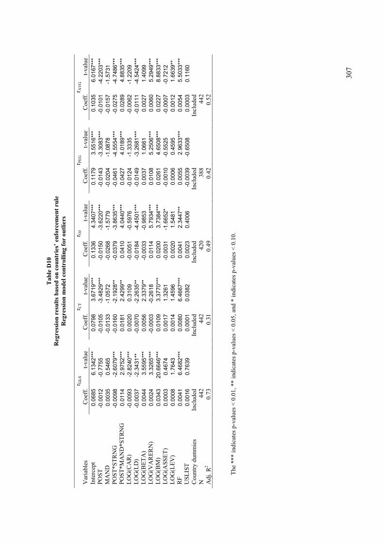
30

7

Table D10


ent rule


r G

LS

r C

T

r O

J

r PE

G

r A

VG

Var

iable

s C

oef

f.

t-val

ue

C

oef

f.

t-val

ue

C

oef

f.

t-val

ue

C

oef

f.

t-val

ue

C

oef

f.

t-val

ue

Inte

rcep

t 0.0685

6.1342***

0.0798

3.6719***

0.1336

4.3407***

0.1179

3.5516***

0.1035

6.0167***

PO

ST

-0.0012

-0.7755***

-0.0105

-3.4829***

-0.0150

-3.6220***

-0.0143

-3.3083***

-0.0101

-4.2203***

MA

ND

0.0035

0.5465***

-0.0133

-1.0572***

-0.0268

-1.5779***

-0.0204

-1.0878***

-0.0157

-1.5731***

PO

ST

*S

TR

NG

-0.0098

-2.6079***

-0.0160

-2.1928***

-0.0379

-3.8635***

-0.0461

-4.5554***

-0.0275

-4.7486***

PO

ST

*M

AN

D*S

TR

NG

0.0114

2.9752***

0.0181

2.4299***

0.0410

4.0440***

0.0427

4.0189***

0.0289

4.8835***

LO

G(C

AR

) -0.0093

-2.8240***

0.0020

0.3109***

-0.0051

-0.5976***

-0.0124

-1.3335***

-0.0062

-1.2209***

LO

G(L

D)

-0.0037

-2.3431***

-0.0070

-2.2635***

-0.0184

-4.4501***

-0.0149

-3.2681***

-0.0111

-4.5424***

LO

G(B

ET

A)

0.0044

3.5595***

0.0056

2.3379***

-0.0033

-0.9853***

0.0037

1.0661***

0.0027

1.4099***

LO

G(V

AR

ER

N)

0.0024

3.3265***

-0.0003

-0.2618***

0.0114

5.7934***

0.0108

5.2506***

0.0060

5.2949***

LO

G(B

M)

0.0343

20.6646***

0.0109

3.3770***

0.0200

3.7384***

0.0261

4.6508***

0.0227

8.8833***

LO

G(A

SS

ET

) 0.0003

0.4674***

0.0017

1.3261***

-0.0031

-1.6652***

-0.0010

-0.5525***

-0.0007

-0.7212***

LO

G(L

EV

) 0.0008

1.7643***

0.0014

1.4596***

0.0020

1.5481***

0.0006

0.4595***

0.0012

1.6639***

RF

0.0041

6.4682***

0.0080

6.4667***

0.0041

2.3447***

0.0055

2.9633***

0.0054

5.5033***

US

LIS

T

0.0016

0.7639***

0.0001

0.0382***

0.0023

0.4006***

-0.0039

-0.6508***

0.0003

0.1160***

Co

un

try d

um

mie

s In

clu

ded

In

clu

ded

In

clu

ded

In

clu

ded

In

clu

ded

N

44

2

442

42

0

38

8

44

2

A

dj.

R2

0.7

3

0.3

1

0.4

9

0.4

2

0.5

2

T

he

*** i

nd

icat

es p

-val

ues

< 0

.01

, ** i

ndic

ates

p-v

alu

es <

0.0

5,

and

* i

ndic

ates

p-v

alu

es <

0.1

0.

30

8

Table D11


ent rule


r G

LS

r C

T

r O

J

r PE

G

r A

VG

Var

iable

s C

oef

f.

t-val

ue

C

oef

f.

t-val

ue

C

oef

f.

t-val

ue

C

oef

f.

t-val

ue

C

oef

f.

t-val

ue

Inte

rcep

t 0.0445

3.3774***

0.0120

0.5032***

0.1008

2.9229***

0.0654

1.7074***

0.0752

3.7298***

PO

ST

-0.0067

-4.2332***

-0.0137

-4.7762***

-0.0139

-3.4484***

-0.0130

-3.1237***

-0.0136

-5.6187***

MA

ND

-0.0008

-0.1073***

0.0128

0.8729***

-0.0371

-1.8388***

-0.0054

-0.2200***

-0.0159

-1.2854***

PO

ST

*S

TR

NG

-0.0082

-2.0567***

-0.0147

-2.0333***

-0.0258

-2.5795***

-0.0324

-3.1643***

-0.0235

-3.8547***

PO

ST

*M

AN

D*S

TR

NG

0.0120

2.9470***

0.0191

2.5818***

0.0297

2.8653***

0.0294

2.7138***

0.0264

4.2265***

CA

R

-0.0307

-1.2165***

0.0763

1.6626***

0.0513

0.8109***

0.0041

0.0615***

0.0231

0.5995***

LD

-0.0014

-2.4274***

-0.0046

-4.2569***

-0.0069

-4.6435***

-0.0076

-4.0278***

-0.0049

-5.3796***

BE

TA

0.0072

3.0844***

0.0033

0.7824***

-0.0064

-1.0825***

0.0060

0.9773***

0.0019

0.5394***

VA

RE

RN

0.0001

1.0972***

-0.0001

-0.5744***

0.0007

2.8536***

0.0007

2.7428***

0.0003

2.4832***

BM

0.0172

18.2738***

0.0001

0.0029***

0.0401

5.0021***

0.0510

6.1032***

0.0092

6.3886***

LO

G(A

SS

ET

) 0.0001

0.1573***

0.0026

2.0666***

-0.0029

-1.5720***

-0.0013

-0.6832***

-0.0008

-0.8265***

LE

V

0.0007

2.6181***

0.0011

2.1660***

0.0010

1.4016***

0.0012

1.4590***

0.0011

2.4648***

RF

0.0065

9.8579***

0.0093

7.8125***

0.0045

2.5246***

0.0063

3.3880***

0.0075

7.4835***

US

LIS

T

0.0029

1.2688***

0.0017

0.4097***

0.0069

1.1630***

-0.0006

-0.0979***

0.0040

1.1164***

LT

G

0.0036

1.7290***

0.0102

2.6459***

-0.0078

-1.4787***

-0.0170

-3.0032***

-0.0004

-0.1348***

Co

un

try d

um

mie

s In

clu

ded

In

clu

ded

In

clu

ded

In

clu

ded

In

clu

ded

N

44

4

444

42

2

39

0

44

4

A

dj.

R2

0.6

9

0.3

2

0.4

8

0.4

2

0.4

6

T

he

*** i

ndic

ates

p-v

alu

es <

0.0

1,

** i

ndic

ates

p-v

alu

es <

0.0

5,

and

* i

ndic

ates

p-v

alu

es <

0.1

0.

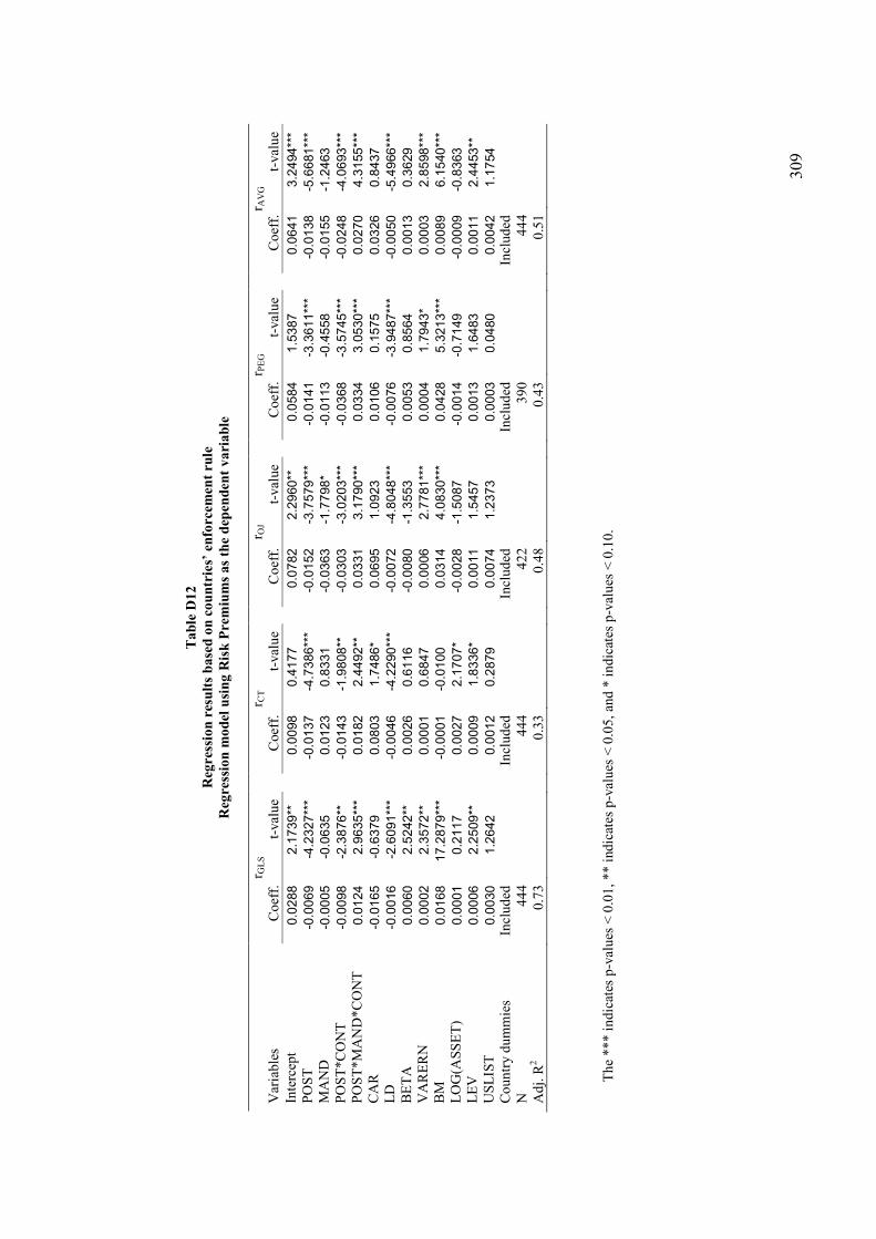
30

9

Table D12


ent rule


r G

LS

r C

T

r O

J

r PE

G

r A

VG

Var

iable

s C

oef

f.

t-val

ue

C

oef

f.

t-val

ue

C

oef

f.

t-val

ue

C

oef

f.

t-val

ue

C

oef

f.

t-val

ue

Inte

rcep

t 0.0288

2.1739***

0.0098

0.4177***

0.0782

2.2960***

0.0584

1.5387***

0.0641

3.2494***

PO

ST

-0.0069

-4.2327***

-0.0137

-4.7386***

-0.0152

-3.7579***

-0.0141

-3.3611***

-0.0138

-5.6681***

MA

ND

-0.0005

-0.0635***

0.0123

0.8331***

-0.0363

-1.7798***

-0.0113

-0.4558***

-0.0155

-1.2463***

PO

ST

*C

ON

T

-0.0098

-2.3876***

-0.0143

-1.9808***

-0.0303

-3.0203***

-0.0368

-3.5745***

-0.0248

-4.0693***

PO

ST

*M

AN

D*C

ON

T

0.0124

2.9635***

0.0182

2.4492***

0.0331

3.1790***

0.0334

3.0530***

0.0270

4.3155***

CA

R

-0.0165

-0.6379***

0.0803

1.7486***

0.0695

1.0923***

0.0106

0.1575***

0.0326

0.8437***

LD

-0.0016

-2.6091***

-0.0046

-4.2290***

-0.0072

-4.8048***

-0.0076

-3.9487***

-0.0050

-5.4966***

BE

TA

0.0060

2.5242***

0.0026

0.6116***

-0.0080

-1.3553***

0.0053

0.8564***

0.0013

0.3629***

VA

RE

RN

0.0002

2.3572***

0.0001

0.6847***

0.0006

2.7781***

0.0004

1.7943***

0.0003

2.8598***

BM

0.0168

17.2879***

-0.0001

-0.0100***

0.0314

4.0830***

0.0428

5.3213***

0.0089

6.1540***

LO

G(A

SS

ET

) 0.0001

0.2117***

0.0027

2.1707***

-0.0028

-1.5087***

-0.0014

-0.7149***

-0.0009

-0.8363***

LE

V

0.0006

2.2509***

0.0009

1.8336***

0.0011

1.5457***

0.0013

1.6483***

0.0011

2.4453***

US

LIS

T

0.0030

1.2642***

0.0012

0.2879***

0.0074

1.2373***

0.0003

0.0480***

0.0042

1.1754***

Co

un

try d

um

mie

s In

clu

ded

In

clu

ded

In

clu

ded

In

clu

ded

In

clu

ded

N

44

4

444

42

2

39

0

44

4

A

dj.

R2

0.7

3

0.3

3

0.4

8

0.4

3

0.5

1

T

he

*** i

ndic

ates

p-v

alu

es <

0.0

1,

** i

ndic

ates

p-v

alu

es <

0.0

5,

and

* i

ndic

ates

p-v

alu

es <

0.1

0.

310

Appendix E

1. Global positions of OTC derivatives markets by type of instrument

The table is a brief reproduction of the Table C.5 in the Triennial Central Bank Survey (BIS, 2007). Amounts outstanding, in billion of US dollars

2. Exchange rates used to translate banks’ accounts into Euros

CURRENCIES 30/12/2005 29/12/2006

CYP - Cyprus Pound 0.5735 0.5782

DKK - Danish Kroner 7.4605 7.4560

GBP - UK pound 0.6853 0.6715

CZK - Czech Koruna 29.0000 27.4850

HUF - Hungarian Forint 252.8700 251.7700

LVL - Latvian Lat 0.6962 0.6972

LTL - Lithuanian Lita 3.4528 3.4528

MTL - Maltese Lira 0.4293 0.4293

RON - Romanian Leu 3.6802 3.3835

SKK - Slovak Koruna 37.8800 34.4350

SIT - Slovenian Tolar 239.5000 239.6400

SEK - Swedish Krona 9.3885 9.0404

USD - US Dollars 1.1797 1.3170

PLN - Polish Zloty 3.8600 3.8310

Notes: 1) Exchange rates are per euro, 2) Data on exchange rates are retrieved from DataStream, and are those provided by ECB on the last available date of each year 2005 and 2006.

Positions at end-June 2004 Positions at end-June 2007

Notional

amounts

Gross market

values

Notional

Amounts

Gross market

values

Foreign exchange contracts 31,500 1,116 57,597 1,611

Interest rate contracts 177,457 4,582 388,627 6,724

Equity-linked contracts 5,094 321 10,760 1,213

Commodity contracts 1,354 176 8,255 690

Credit derivatives 4,474 131 51,095 906

Other derivatives 191 65 78 1

Total contacts 220,070 6,391 516,412 11,145

311

References

Aboody, D., Barth, M. E., & Kasznik, R. (1999). Revaluations of fixed assets and future firm performance: Evidence from the UK. Journal of Accounting and Economics, 26: 149-178.

Aboody, D., & Lev, B. (1998). The value relevance of intangibles: The case of software

capitalization. Journal of Accounting Research, 36(Supplement): 161-191. Agung, I. G. N., (2009). Time series data analysis using Eviews. Singapore: John Wiley & Sons

(Asia) Pte Ltd. Ahmed, A. S., Kilic, E., & Lobo, G. J. (2006). Does recognition versus disclosure matter?

Evidence from value-relevance of banks' recognized and disclosed derivative financial instruments. The Accounting Review, 81(3): 567-588.

Ahmed, A. S., & Takeda, C. (1995). Stock market valuation of gains and losses on commercial

banks' investment securities An empirical analysis. Journal of Accounting and Economics, 20: 207-225.

Alford, A., Jones, J., Leftwich, R. & Zmijewski M. (1993). The relative informativeness of

accounting disclosures in different countries. Journal of Accounting Research, 31: 183-223.

Ali, A. & Hwang Lee-Seok. (2000). Country-specific factors related to financial reporting and the value relevance of accounting data. Journal of Accounting Research, 38(1): 1-21.

American Accounting Association (AAA) Financial Accounting Standards Committee (FASC).

(1998) Response to a discussion paper issued by the IASC/CICA Streering Committee on Financial Instruments, "Accounting for financial assets and financial liabilities" Accounting Horizons, 12(March): 90-97.

Amihud. Y, & Mendelson, H. (1986). Asset Pricing and the Bid-ask Spread. Journal of

Financial Economics: 223-49. Armstrong, C. S., Barth, M. E., & Riedl, E. J. (2010). Market reaction to the adoption of IFRS in

Europe. The Accounting Review, 85(1): 31-61. Ashbaugh, H., & Pincus, M. (2001). Domestic accounting standards, International Accounting

Standards, and the predictability of earnings. Journal of Accounting Research, 39(3): 417-434.

Ball, R. (2006). International Financial Reporting Standards (IFRS): pros and cons for investors.

Accounting and Business Research, 36(Special Issue): 5-27.

312

Barry, C. B. & Brown, S. J. (1985). Differential information and security market equilibrium. Journal of Financial and Quantitative Analysis. 20(4): 407-422.

Barker, R. (2001). Determining Value: valuation models and financial statements: Essex:

Pearson Education Limited. Barth, M. E. (1991). Relative measurement errors among alternative pension asset and liability

measures. The Accounting Review, 66(3): 433-463. Barth, M. E. (1994). Fair value accounting: Evidence from investment securities and the market

valuation of banks. The Accounting Review, 69(1): 1-25. Barth, M. E. (2000). Valuation-based accounting research: Implications for financial reporting

and opportunities for future research. Accounting and Finance, 40: 7-31. Barth, M. E. (2006a). Including estimates of the future in today's financial statements.

Accounting Horizons, 20(3): 271-285. Barth, M. E. (2006b). Research, Standard Setting, and Global Financial Reporting. Foundations

and Trends in Accounting, 1(2): 71-165. Barth, M. E. (2007). Standard-setting measurement issues and the relevance of research.

Accounting and Business Research, Special Issue: 7-15. Barth, M. E., Beaver, W. H., & Landsman, W. R. (1996). Value-relevance of banks' fair value

disclosures under SFAS No. 107. The Accounting Review, 71(4): 513-537. Barth, M. E., Beaver, W. H., & Landsman, W. R. (2001). The relevance of the value relevance

literature for financial accounting standard setting - another view. Journal of Accounting and Economics, 31: 77-104.

Barth, M. E., & Callapur, S. (1996). The effects of cross-sectional scale differences on regression

results in empirical accounting research. Contemporary Accounting Research, 13(2): 527-567.

Barth, M. E., & Clinch, G. (1998). Revalued financial, tangible and intangible assets:

Associations with share prices and non-market-based value estimates. Journal of Accounting Research, 36(Supplement): 199-233.

Barth, M. E., Landsman, W. R., & Lang, M. H. (2008). International Accounting Standards and

accounting quality. Journal of Accounting Research, 46(3): 467-498. Barton. (2001). Does the use of financial derivatives affect earnings management decisions? The

Accounting Review, 76(1): 1-26.

313

Beaver, W. (1998). Financial reporting: an accounting revolution (3rd ed.): New Jersey: Prentice-Hall, Upper Saddle River.

Beaver, W. (2002). Perspectives on recent capital market research. The Accounting Review,

77(2): 453-474. Beaver, W., Eger, C., Ryan, S., & Wolfson, M. (1989). Financial reporting, supplemental

disclosures, and bank share prices. Journal of Accounting Research, 27(2): 157-178. Beaver, W., Kettler, P., & Scholes, M. (1970). The association between market determined and

accounting determined risk measures. The Accounting Review, 45(4): 654-682. Bernard, V. L., Merton, R. C., & Palepu, K. G. (1995). Mark-to-market accounting for banks and

thrifts: Lessons from the Danish experience Journal of Accounting Research, 33(1): 1-32.

BIS (2004a). Comments on the IAS 39 fair value option proposal. Bank for International

Settlements: Basel, Switzerland. BIS (2004b). International Convergence of Capital Measurement and Capital Standards: a

Revised Framework. Bank for International Settlements: Basel, Switzerland. BIS. (2007). Foreign exchange and derivatives market activity in 2007. Bank for International

Settlements, Triennial Central Bank Survey: Basel, Switzerland. Botosan, C. A. (1997). Disclosure level and the cost of equity capital. The Accounting Review,

72(3): 323-349. Botosan, C. A. (2006). Disclosure and the cost of capital: what do we know? Accounting and

Business Research. International Accounting Policy Forum: 31-40. Botosan, C. A., & Plumlee, M. A. (2002). A re-examination of disclosure level and the expected

cost of equity capital. Journal of Accounting Research, 40(1): 21-40. Burgstahler, D. C., Hail, L., & Leuz, C. (2006). The importance of reporting incentives: Earnings

management in European private and Public Firms. The Accounting Review, 81(5): 983-1016.

Butler, C. (2009). Accounting for financial instruments. West Sussex: John Wiley & Sons Ltd. Carhart, M. M. (1997). On persistence in mutual fund performance. The Journal of Finance,

52(1): 57-82. Carroll, T. J., Linsmeier, T. J., & Petroni, K. R. (2003). The reliability of fair value versus

historical cost information: Evidence from closed-end mutual funds. Journal of Accounting, Auditing & Finance, 18(1): 1-23.

314

Carter, D. A. & Sinkey, J. F. (1998). The use of interest rate derivatives by end-users: The case

of Large Community banks. Journal of Financial Services Research, 14(1): 17-34. Casu, B., Girardone, C., & Molyneux, P. (2006). Introduction to banking: Essex: Pearson

Education Limited. Choi, F. D. S. (1973). Financial disclosure in relation to a firm's capital costs. Accounting and

Business Research, 75(Autumn). Christensen, H.B., Lee, E. & Walker, M. (2007). Cross-sectional variation in the economic

consequences of international accounting harmonization: The case of mandatory IFRS adoption in the UK. The International Journal of Accounting, 42: 341-379.

Christensen, H.B. & Nikolaev, V. (2009). Who uses fair value accounting for non-financial

assets after IFRS adoption? Working Paper No. 09-12: The University of Chicago, Booth School of Business.

Christie, A. A. (1987). On Cross-Sectional Analysis in Accounting Research. Journal of

Accounting and Economics, 9(3): 231-258. Claus, J., & Thomas, J. (2001). Equity premia as low as three percent? Evidence from analysts'

earnings forecasts for domestic and international stock markets. The Journal of Finance, 56(5): 1629-1666.

Coles, J. F., Loewenstein, & Suay, J. (1995). On equilibrium pricing under parameter uncertainty.

Journal of Financial and Quantitative Analysis, 30(3): 347-364. Collins, D. W., & Kothari, S. P. (1989). An analysis of intertemporal and cross-sectional

determinants of earnings response coefficients. Journal of Accounting and Economics, 11(3): 143-181.

Cuijpers, R., & Buijink, W. (2005). Voluntary Adoption of Non-local GAAP in the European

Union: A study of determinants and consequences. European Accounting Review, 14(3): 487-524.

Damodaran, A. (2002). Investment Valuation (2nd ed.). New York: John Wiley & Sons, Inc. Danbolt, J. & Rees, W. (2008). An Experiment in Fair Value Accounting: UK Investment

Vehicles. European Accounting Review, 17(2): 271-303. Dargenidou, C., Mcleay, S. & Raonic, I. (2006). Expected Earnings Growth and the Cost of

Capital: An Analysis of Accounting Regime Change in the European Financial Market. Abacus, 42(3/4): 388-414.

315

Daske, H. (2006). Economic benefits of adopting IFRS or US-GAAP - Have the expected cost of equity capital really decreased? Journal of Business, Finance & Accounting, 33(3&4): 329-373.

Daske, H., Hail, L., Leuz, C., & Verdi, R. (2007). Adopting a Label: Heterogeneity in the

Economic Consequences of IFRS Adoptions. Available at SSRN. Daske, H., Hail, L., Leuz, C., & Verdi, R. (2008). Mandatory IFRS reporting around the word:

Early evidence on the economic consequences. Journal of Accounting Research, 46(5): 1085-1142.

Demirguc Kunt, A., Karacaovali, B., & Laeven, L. (2005). Deposit insurance around the world:

A comprehensive datadase, World Bank Research Working Paper. Dhaliwal, D., Krull, L., & Li, O. Z. (2007). Did the 2003 Tax Act reduce the cost of equity

capital? Journal of Accounting and Economics, 43: 121-150. Dhaliwal, D. S. (1979). Disclosure regulations and the cost of capital. Southern Economic

Journal, 45(3): 785-794. Dhaliwal, D. S., Spicer, B. H., & Vickrey, D. (1979). The quality of disclosure and the cost of

capital. Journal of Business, Finance & Accounting, 6(2): 245-266. Diamond, D. W., & Verrecchia, R. E. (1991). Disclosure, Liquidity, and the cost of capital. The

Journal of Finance, 46(4): 1325-1359. Dietrich, J. R., Harris, M. S. & Muller III, K. A. (2001). The reliability of investment property

fair value estimates. Journal of Accounting and Economics, 30: 125-158. Easley, D., & M. O’Hara. 2004. Information and the cost of capital. The Journal of Finance, 59

(4): 1553–1583. Easton, P.D., Taylor, G., Shroff, P., & Sougiannis, T. (2002). Using forecasts of earnings to

simultaneously estimate growth and the rate of return on equity investment. Journal of Accounting Research, 40(3): 657-676.

Easton, P. D. (2004). PE ratios, PEG ratios, and estimating the implied expected rate of return on

equity capital. The Accounting Review, 79(1): 73-95. Easton, P. D., Eddey, P. H. & Harris, T. S. (1993). An investigation of revaluations of tangible

long-lived assets. Journal of Accounting Research, 31: 1-38. Easton, P. D., & Zmijewski, M. E. (1989). Cross-sectional variation in the stock market response

to the announcement of accounting earnings. Journal of Accounting and Economics, 11: 117-141.

316

Eccher, E. A., Ramesh, K., & Thiagarajan, S. R. (1996). Fair value disclosures by bank holding companies. Journal of Accounting and Economics, 22(1-3): 79-117.

Edey, H. (1962). Business valuation, goodwill and the super-profit method: in Baxter, W. and

Davidson, S. (Eds) Studies in accounting theory, Sweet and Maxwell, London. Edwards, E. O., & Bell, P. W. (1961). The theory and measurement of business income.

Berkeley: California University Press. EBF. (2003). FBE Comments on the proposed amendments to IAS 39 financial instruments

“recognition and measurement – fair value hedge accounting for a portfolio hedge

of interest rate risk”. European Banking Federation: Brussels, Belgium. Fabozzi, F. J. (2002). The handbook of financial instruments. Hoboken, New Jersey: John

Wiley & Sons, Inc. Fama, E. F., & French, K. R. (1993). Common risk factors in the returns on stocks and bonds.

Journal of Financial Economics, 33(1): 3-56. Fama, E. F., & French, K. R. (1995). Size and Book-to-Market factors in earnings and returns.

The Journal of Finance, 50(1): 131-155. Fama, E. F., & French, K. R. (1996). Multifactor explanations of asset pricing anomalies. The

Journal of Finance, 51(1): 55-84. Fama, E. F., & French, K. R. (2004). The Capital Asset Pricing Model: Theory and Evidence.

Journal of Economic Perspectives, 18(3): 25-46. Fama, E. F., & Roll, R. (1968). Some properties of symmetric stable distributions. Journal of

the American Statistical Association, 63(323): 817-836. FASB. (1974). Statement of Financial Accounting Standards No. 2, Accounting for Research

and Development Costs. Financial Accounting Standards Board: Norwalk, Connecticut. FASB. (1985). Statement of Financial Accounting Standards No. 86, Accounting for the Costs

of Computer Software to Be Sold, Leased, or Otherwise Marketed. Financial Accounting Standards Board: Norwalk, Connecticut.

FASB. (1985). Statement of Financial Accounting Standards No. 87, Employers’ Accounting

for Pensions. Financial Accounting Standards Board: Norwalk, Connecticut. FASB. (1990). Statement of Financial Accounting Standards No. 105, Disclosure of

Information about Financial Instruments with Off-Balance-Sheet Risk and Financial

Instruments with Concentrations of Credit Risk. Financial Accounting Standards Board: Norwalk, Connecticut.

317

FASB. (1991). Statement of Financial Accounting Standards No. 107, Disclosures about Fair Value of Financial Instruments. Financial Accounting Standards Board: Norwalk, Connecticut.

FASB. (1993). Statement of Financial Accounting Standards No. 115, Accounting for Certain

Investments in Debt and Equity Securities. Financial Accounting Standards Board: Norwalk, Connecticut.

FASB. (1994). Statement of Financial Accounting Standards No. 119, Disclosure about

Derivative Financial Instruments and Fair Value of Financial Instruments. Financial Accounting Standards Board: Norwalk, Connecticut.

FASB. (1998). Statement of Financial Accounting Standards No. 133, Accounting for

Derivative Instruments and Hedging Activities. Financial Accounting Standards Board: Norwalk, Connecticut.

FASB. (2006). Statement of Financial Accounting Standards No. 157, Fair Value

Measurements. Financial Accounting Standards Board: Norwalk, Connecticut. FASB. (2007). Statement of Financial Accounting Standards No. 159, The Fair Value Option

for Financial Assets and Financial Liabilities—Including an amendment of FASB

Statement No. 115. Financial Accounting Standards Board: Norwalk, Connecticut. Feltham, G. A., & Ohlson, J. A. (1995). Valuation and clean surplus accounting for operating

and financial activities. Contemporary Accounting Research, 11(Spring): 689-731. Flannery, M. J., & James, C. M. (1984a). The effect of interest rate changes on the common

stock returns of financial institutions The Journal of Finance, 39(4): 1141-1153. Flannery, M. J., & James, C. M. (1984b). Market evidence on the effective maturity of bank

assets and liabilities. Journal of Money, Credit, and Banking, 16(4): 435-445. Francis, J., Nanda, D., & Olsson, P. (2008). Voluntary disclosure, earnings quality, and cost of

capital. Journal of Accounting Research, 46(1): 53-99. Frankel, R., & Lee, C. M. C. (1998). Accounting valuation, market expectation, and cross-

sectional stock returns. Journal of Accounting and Economics, 25(3): 283-319. Gebhardt, W. R., Lee, C. M. C., & Swaminathan, B. (2001). Toward an implied cost of capital.

Journal of Accounting Research, 39(1): 135-176. Geczy, C., Minton, B. A., & Schrand, C. (1997). Why firms use currency derivatives. The

Journal of Finance, 52(4): 1323-1354. Gode, D., & Mohanram, P. (2003). Inferring the cost of capital using the Ohlson-Juettner model.

Review of Accounting Studies, 8: 399-431.

318

Goh, B. W., Ng, J. & Yong, K. O. (2009). Market Pricing of Banks' Fair Value Assets

Reported under SFAS 157 During the 2008 Economic Crisis. Available at SSRN: http://ssrn.com/abstract=1335848.

Graham, R. C., Lefanowicz, C. E., & Petroni, K. R. (2003). The value relevance of equity

method fair value disclosures. Journal of Business, Finance, and Accounting, 30(7-8): 1065-1088.

Greene, W. H. (2002). Econometric Analysis (5th ed.). Upper Saddle River, New Jersey:

Pearson Education, Inc. Hail, L. (2002). The impact of voluntary corporate disclosures on the ex-ante cost of capital for

Swiss firms. The European Accounting Review, 11(4): 741-773. Hail, L., & Leuz, C. (2006). International differences in the cost of equity capital: Do legal

institutions and securities regulation matter. Journal of Accounting Research, 44(3): 485-531.

Hail, L., Leuz, C. & Wysocki P. (2010). Global Accounting Convergence and the Potential

Adoption of IFRS by the U.S. (Part I): Conceptual Underpinnings and Economic Analysis. Accounting Horizons, 24(3): 355-394.

Healy, P. M., & Palepu, K. G. (2001). Information asymmetry, corporate disclosure, and the

capital markets: A review of the empirical disclosure literature. Journal of Accounting and Economics, 31: 405-440.

Holthausen, R. W., & Watts, R. L. (2001). The relevance of the value relevance literature for

financial accounting standard setting. Journal of Accounting and Economics, 31: 3-75. Horngren, C. T. 1957. Disclosure: (1957). The Accounting Review, 32(4): 598-604. Hung, M. (2001). Accounting standards and value relevance of financial statements: An

international analysis. Journal of Accounting and Economics, 30: 401-420. IASB. (1998). Provisions, Contingent Liabilities and Contingent Assets. London: International

Accounting Standards Board. IASB. (2000a). International Accounting Standard 30: Disclosures in Financial Statements of

Banks and Similar Financial Institutions. London: International Accounting Standards Board.

IASB. (2000b). International Accounting Standard 40: Investment Property. London:

International Accounting Standards Board.

319

IASB. (2003a). International Accounting Standard 32: Financial Instruments: Disclosure and Presentation. London: International Accounting Standards Board.

IASB. (2003b). International Accounting Standard 39: Financial Instruments: Recognition

and Measurement. London: International Accounting Standards Board. IASB. (2005). International Financial Reporting Standard 7: Financial Instruments:

Disclosures. London: International Accounting Standards Board. IASB. (2008). Discussion Paper: Reducing Complexity in Reporting Financial Instruments.

London: International Accounting Standards Board. IASB. (2009). International Financial Reporting Standard 9: Financial Instruments. London:

International Accounting Standards Board. IASB. (2010). The Conceptual Framework for Financial Reporting. International Accounting

Standards Committee: London, UK. IASCF. (2003). Annual Report 2002. International Accounting Standards Committee

Foundation: London, UK. Jegadeesh, N., & Titman, S. (1993). Returns to buying winners and selling losers: Implications

for stock market efficiency The Journal of Finance, 48(1): 65-91. Karels, G. V., Prakash, A. J., & Roussakis, E. (1989). The relationship between bank capital

adequacy and market measures of risk. Journal of Business, Finance & Accounting, 16(5): 663-673.

Kaufmann, D., Kraay, A., & Mastruzzi, M. (2009). Governance Matters VIII: Aggregate and

Individual Governance Indicators 1996-2008, Global Governance Program: The World Bank.

Khurana, I. K., & Kim, M. (2003). Relative value relevance of historical cost vs. Fair value:

Evidence from bank holding companies, Journal of Accounting and Public Policy, 22(1): 19-42.

Kolev, K. (2008). Do Investors Perceive Marking-to-Model as Marking-to-Myth? Early

Evidence from FAS 157 Disclosure. Available at SSRN: http://ssrn.com/abstract=1336368.

Kousenidis, D. V., Ladas, A. C., & Negakis, C. I. (2010) Value relevance of accounting

information in the pre- and post-IFRS accounting periods. European Research Studies, 13(1): 143-152.

La Porta, R., Lopez-de-Silanes, F., & Shleifer, A. (1998). Law and finance. Journal of Political

Economy, 106: 1113-1155.

320

La Porta, R., Lopez-De-Silanes, F., Shleifer, A., & Vishny, R. W. (1997). Legal determinants of

external finance The Journal of Finance, 52(3): 1131-1150. Landsman, W. R. (1986). An empirical investigation of pension fund property rights. The

Accounting Review, 61(4): 662-691. Landsman, W. R., & Magliolo, J. (1988). Cross-sectional capital market research and model

specification. The Accounting Review, 63(4): 586-604. Landsman, W. R. (2007). Is fair value accounting information relevant and reliable? Evidence

from capital market research. Accounting and Business Research, Special Issue: 19-30. Larcker, D. F., & Rusticus, T. O. (2010). On the use of instrumental variables in accounting

research. Journal of Accounting and Economics, 49(3): 186-205. Lee, C. M. C. (1999). Accounting-based valuation: Impact on business practices and research.

Accounting Horizons, 13(4): 413-425. Lee, E., Walker, M., and Christensen, H. B. (2008). Mandating IFRS: Its impact on the cost of

equity capital in Europe. Research Report 105. London: The Association of Chartered Certified Accountants.

Leuz, C. (2003). IAS versus U.S. GAAP: Information asymmetry-based evidence from

Germany's New Market. Journal of Accounting Research, 41(3): 445-472. Leuz, C., Nanda, D., & Wysocki, P. D. (2003). Earnings management and investor protection: an

international comparison. Journal of Financial Economics, 69(3): 505-527. Leuz, C., & Verrecchia, R. E. (2000). The economic consequences of increased disclosure.

Journal of Accounting Research, 38(Supplement): 91-124. Lev, B., & Sougiannis, T. (1996). The capitalization, amortization, and value-relevance of R&D.

Journal of Accounting and Economics, 21: 107-138. Levitt, A. (1998). The importance of high quality accounting standards. Accounting Horizons,

12(1): 79-82. Li, S. (2010). Does mandatory adoption of International Financial Reporting Standards in the

European Union reduce the cost of equity capital? The Accounting Review, 85(2): 607-636.

Lintner, J. (1965). The valuation of risky assets and the selection of risky investments in stock

portfolios and capital budgets. Review of Economics and Statistics, 47: 13-37.

321

Lo, K., & Lys, T. (2000). The Ohlson model: Contribution to valuation theory, limitations, and empirical applications. Journal of Accounting, Auditing & Finance, 15(3): 337-367.

Mansur, I., Zangeneh, H., & Zitz, M. S. (1993). The association between banks' performance

ratios and market-determined measures of risk. Applied Economics, 25: 1503-1510. Markowitz, H. (1959). Portfolio selection: Efficient diversification of investments. New York:

John Wiley. Modigliani, F. & Miller, M. H. (1958). The cost of capital, corporation finance and the theory of

investment. The American Economic Review, 48(3): 261-297. Nelson, K. K. (1996). Fair value accounting for commercial banks: An empirical analysis of

SFAS No. 107. The Accounting Review, 71(2): 161-182. Nobes, C. (2001). GAAP 2001: A Survey of National Accounting Rules Benchmarked

Against International Accounting Standards by Andersen, BDO, Deloitte Touche

Tohmatsu, Ernst & Young, Grant Thornton, KPMG, PricewaterhouseCoopers. New York, NY: J Wiley & Sons.

Nobes, C. (2008). Accounting classification in the IFRS era. Australian Accounting Review,

18(3): 191-198. Ohlson, J. A. (1995). Earnings, book values, and dividends in equity valuation. Contemporary

Accounting Research, 11(2): 661-687. Ohlson, J. A., & Juettner-Nauroth, B. (2005). Expected EPS and EPS Growth as determinants of

value Review of Accounting Studies, 10: 349-365. Owusu-Ansah, S. & Yeoh, J. (2006). Relative Value Relevance of Alternative Accounting

Treatments for Unrealized Gains: Implications for the IASB. Journal of International Financial Management and Accounting, 17(3): 228-255.

Park, M. S., Park, T., & Ro, B. T. (1999). Fair value disclosures for investment securities and

bank equity: Evidence from SFAS No. 115. Journal of Accounting, Auditing & Finance, 14(3): 347-370.

Pastor, L., & Stambaugh, R. F. (1999). Costs of equity capital and model mispricing. The

Journal of Finance, 54(1): 67-121. Peasnell, K. V. (1982). Some formal connections between economic values and yields and

accounting numbers. Journal of Business, Finance & Accounting, 9(3): 361-381. Penman, S. H. (2007). Financial reporting quality: is fair value a plus or a minus? Accounting

and Business Research, 37 (Special Issue): 33-44.

322

Petroni, K. R., & Wahlen, J. M. (1995). Fair values of equity and debt securities and share prices of Property-Liability Insurers. The Journal of Risk and Insurance, 62(4): 719-737.

Poshakwale, S., & Courtis, J. K. (2005). Disclosure level and cost of equity capital: Evidence

from the banking industry. Managerial And Decision Economics, 26: 431-444. Preinreich, G. A. D. (1938). Annual survey of economic theory: The theory of depreciation

Econometrica, 6(3): 219-241. Ray, K. (2010). One size fits all? Costs and benefits of uniform accounting standards. Working

Paper, Georgetown University: McDonough School of Business. Rees, W. P. (1995). Financial Analysis (2nd ed.): Hemel Hempstead: Prentice Hall International. Richardson, A. J., & Welker, M. (2001). Social disclosure, financial disclosure and the cost of

equity capital. Accounting, Organizations and Society, 26: 597-616. Riffe, S. (1997). The valuation of off-balance-sheet financial instrument disclosures in the

banking industry. In B. Schachter (Ed.), Derivatives, regulation and banking: advances in finance, investment and banking series: 93-121. Amsterdam: North-Holland.

Ruland, W., Shon, J., & Zhou, P. (2007). Effective controls for research in international

accounting. Journal of Accounting and Public Policy: 26: 96-116. Ryan, S. G. (1999). Discussion: “Fair value disclosures for investment securities and bank equity:

Evidence from SFAS No. 115”. Journal of Accounting, Auditing & Finance, 14(3): 371-377.

Ryan, S. G. (2007). Financial Instruments & Institutions: Accounting and disclosure rules

(Second ed.). Hoboken, New Jersey: John Wiley & Sons, Inc. Seow, G. S. & Tam, K. The usefulness of derivative-related accounting disclosures. Review of

quantitative finance and accounting, 18(3): 273-291. Sharpe, W. (1964). Capital asset prices: A theory of market equilibrium under conditions of risk.

Journal of Finance, 19: 425-442. Simko, P. J. (1999). Financial instrument fair values and nonfinancial firms. Journal of

Accounting, Auditing & Finance, 14(3): 247-274. Skinner, D. J. (1996). Are disclosures about bank derivatives and employee stock options 'value-

relevant'? Journal of Accounting and Economics, 22: 393-405. So, S. & Smith, M. (2009). Value-relevance of presenting changes in fair value of investment

properties in the income statement: evidence from Hong Kong. Accounting and Business Research, 39(2): 103-118.

323

Song, C. J., Thomas, W. B. & Yi, H. (2010). Value Relevance of FAS No. 157 FairValue

Hierarchy Information and the Impact of Corporate Governance Mechanisms. The Accounting Review, 85(4): 1375-1410.

Venkatachalam, M. (1996). Value-relevance of banks' derivatives disclosures. Journal of

Accounting and Economics, 22(1-3): 327-355. Wang, L., Alam, P., & Makar, S. (2005). The value-relevance of derivative disclosures by

commercial banks: A comprehensive study of information content under SFAS Nos. 119 and 133. Review of Quantitative Finance and Accounting, 25: 413-427.

Watts, R. L., & Zimmerman, J. L. (1986). Positive Accounting Theory. Englewood Cliffs, NJ:

Prentice Hall. Wetmore, J. L. (2004). Panel Data, liquidity risk, and increasing Loans-to-Core Deposits ratio of

large commercial bank holding companies [1992-2000]. American Business Review, 22(2): 99-107.

White, H. (1980). A heteroskedasticity-consistent covariance matrix estimator and a direct test

for heteroskedasticity. Econometrica, 48(4): 817-838. Whittington, G. (2005). The adoption of International Accounting Standards in the European

Union. European Accounting Review, 14(1): 127-153. Williams, J. B. (1938). The theory of investment value. Cambridge: MA Harvard University

Press. Wooldridge, J. M. (2006). Introductory Econometrics (3rd ed.), USA: Thomson South-Western. Zeff, S. A. (2007). Some obstacles to global financial reporting comparability and converge at a

high level of quality. The British Accounting Review, 39(4): 290-302.

IFRS and European Commercial Banks: Value Relevance and ...

Documents

Transcript of IFRS and European Commercial Banks: Value Relevance and ...