ifo WORKING PAPERS

204Update

March 2018

Petrodollar Recycling, Oil Monopoly, and Carbon Taxes Waldemar Marz, Johannes Pfeiffer

ifo Working Paper No. 204

Petrodollar Recycling, Oil Monopoly, and Carbon Taxes*

Abstract We identify a new general equilibrium transmission channel of climate policy on oil extraction, assuming an oil monopolist who accounts for the implications of oil supply on her capital asset returns. Policy-induced adjustments in asset holdings lead to postponement of extraction under a wide range of reasonable parameter settings: present extraction can drop considerably for a moderately high carbon tax. For endogenous exploration, a decrease in first-period extraction and in cumulative extraction at the same time is also possible. This contrasts with the literature on supply-side effects of climate policy which neglects these capital market implications. Concerns about carbon taxes arising from impeding climate-damaging supply reactions are alleviated, while taxing asset returns may induce acceleration of extraction. JEL code: D90; H20; Q31; Q38 Keywords: Monopoly, fossil energy resources, general equilibrium, capital market, climate policy

Waldemar Marz ifo Institute – Leibniz Institute for

Economic Research at the University of Munich,

University of Munich Poschingerstr. 5

81679 Munich, Germany Phone: + 49 89 9224 1244

marz@ifo.de

Johannes Pfeiffer ifo Institute – Leibniz Institute for

Economic Research at the University of Munich,

University of Munich Poschingerstr. 5

81679 Munich, Germany Phone: + 49 89 9224 1238

pfeiffer@ifo.de

This version: 31 March 2018 First draft: September 2015 * This work was supported by the German Federal Ministry of Education and Research (Project No. 01LA1120A). **Corresponding author.

1 Introduction

In the first half of 2016, Saudi Deputy Crown Prince Mohammad bin Salman, entrusted

with Saudi Arabian long-term oil extraction policy, announced a plan to make his country

economically independent of oil by 2030. To achieve this, the Saudi government intends

to establish the so far largest sovereign wealth fund of US $2 trillion. By investing heavily

in all sorts of capital assets, the prince wants to make "investments the source of Saudi

government revenue, not oil" (Waldman 2016). Other OPEC countries have also been

keeping oil wealth in sovereign wealth funds for many years: As of 2016 Abu Dhabi

holds US $792 billion in such funds, Kuwait holds US $592 billion, and Qatar holds US

$256 billion (SWFI 2016).1 OPEC countries appear to be pursuing a two-pillar supply

strategy: While they continue to be suppliers of oil, the prince’s plan suggests that in the

decades to come, they will be shifting toward income from capital assets to prepare for a

future post-oil world. The two strategic pillars – oil revenues and capital asset returns –

are intertwined by a complex interplay of the oil market and the capital market. The oil

price plays a central role in the world economy and can heavily affect the business cycle

and the resulting returns for stock- and bondholders, especially in the major oil importing

countries.2 Moreover, long-term paths of economic growth and capital accumulation are

affected by the availability of oil.3 Fast-growing emerging economies like China, in turn,

have a significant impact on oil demand and prices.4

At the same time, growing concern over climate change drives attempts to limit global

carbon emissions and potentially dangerous mean temperature increases, such as the 2015

Paris Agreement. Naturally, these attempts threaten the oil exporters’ revenues. So, for

1 As of August 2016, the total volume of oil- and gas-related publicly known sovereign wealth funds wasUS $4,205 billion (SWFI 2016).

2 Cf. Hamilton (1983, 2013), Kang et al. (2014), Cunado and Perez de Gracia (2014). Kilian (2009)points out in his econometric study that the magnitude of macroeconomic effects of an oil price shockdepends on whether it is driven by the supply side, the demand side, or demand-side responses to ananticipated supply shock.

3 Cf., from an empirical perspective, Berk and Yetkiner (2014) and Stern and Kander (2012); from atheoretical perspective, see Stiglitz (1974).

4 Cf. Kilian and Hicks (2013) and Fouquet (2014).

1

climate policy to be effective, strategic reactions of suppliers of fossil fuels like oil must be

taken into account. But, to date, there has been no systematic analysis of climate policy

response by an oil supplier with market power5 that takes into account the two-pillar

nature of OPEC countries’ strategic behavior and the interplay between both markets.

We analyze the extraction reaction of an oil monopolist with capital investments in the

oil importing country to the introduction or increase of a carbon tax on oil imports

in a two-country setting. We apply a general equilibrium approach to incorporate the

interplay between the oil market and the capital market and to capture the crucial role

of capital assets for an oil monopolist’s climate policy reaction, which has been neglected

in the literature to date. In doing so, we find a new channel for postponement instead

of acceleration of oil extraction, due to tightening climate policy. In the literature on

the supply-side of fossil fuel markets it has been pointed out that even the credible

announcement of climate policies that are tightened over time could very well cause the

opposite of the intended effect. The dire prospects for future profits would lead fossil fuel

exporters to accelerate extraction in the present and thereby exacerbate climate-change-

related damages, which is called the "Green Paradox".

In our general equilibrium model we distinguish between one country that only exports oil

and another that imports oil and produces final goods. The time horizon is finite with two

periods and we model climate policy with a carbon tax on oil imports. The interest rate

and savings, which determine physical capital accumulation, are endogenously affected

by oil supply, while the resulting capital stock drives oil demand and revenues for the

exporting countries. We build on the scarce literature on fossil resource monopoly in

general equilibrium6, and especially on the framework and crucial role of capital assets

in Marz and Pfeiffer (2015).7 In the present paper, we introduce climate policy into this

5 There are, of course, many suppliers of oil in the world. But the market share of OPEC, which,according to the International Energy Agency, was 42% in 2013 and 48% in 2040 under the 450ppmcarbon scenario (OECD 2014, p. 115, table 3.5), seems to suggest a significant degree of market powerin the oil market. We focus on a pure monopoly as the opposite to perfect competition.

6 Cf. Moussavian and Samuelson (1984) and Hillman and Long (1985), neither of whom considersclimate policy.

7 Marz and Pfeiffer (2015) show (without discussing climate policy) that the interaction of the capital

2

framework and analyze its implications for the monopolist’s oil supply behavior.

Our key finding is that the simultaneous consideration of oil revenues and capital income

gives rise to a new channel for postponement of extraction: The expected income loss

due to future oil taxation leads the oil-rich country to increase its savings. This boosts

the monopolist’s capital asset motive in period 2 and creates an incentive to postpone oil

extraction that can dominate the conventional acceleration incentive. In fact, postpone-

ment of extraction can be observed numerically for a wide range of plausible parameter

settings. The magnitude of postponement can be considerable: In certain parameter

settings present extraction drops by almost 30% for a future ad-valorem carbon tax cor-

responding to a carbon price of about 80 dollars per ton of carbon. The latter number is

in line with estimates for the social cost of carbon by Anthoff et al. (2009) or Nordhaus

(2010) and lies roughly in the middle of the wide range of estimates. Overall, we show

that (even) an over time increasing carbon tax can be a viable policy option in contrast to

conventional partial equilibrium analyses of climate policy instruments. Moreover, Sinn

(2008) suggested a capital income tax to circumvent a potential acceleration reaction. In

our framework with its emphasis on capital assets, however, we find that a capital in-

come tax is no longer immune against undesired acceleration of extraction. Endogenizing

cumulative extraction we identify another implication of the interaction of the capital

and the resource market in general equilibrium: capital accumulation depends on the

exploration investment decision. Accounting for this relationship, the monopolist may

choose to reduce cumulative extraction even when reducing first period resource supply.

Our paper contributes to the literature on the supply-side reaction of fossil energy re-

and the resource market already has implications for the supply decision of a resource owner withmarket power if the monopolist is aware of the more widespread effects of resource supply in a generalequilibrium setting (cf. also Bonanno (1990)). More specifically, additional supply motives arise fromthe interaction of these markets in general equilibrium and from the complementarity of physicalcapital and the fossil resource in final goods production. In particular, the monopolist takes intoaccount the influence of resource supply on the return of her own capital assets, which are investedin the oil importing countries, and on capital accumulation with resulting feedbacks on capital andresource demand. Higgins et al. (2006) conclude that about half of the oil exporting countries’ profitsin the 2000s were invested in foreign assets and over different channels ended up in the U.S. In contrastto the conventional partial equilibrium view (cf. Stiglitz 1976) the arising general equilibrium supplymotives mentioned above additionally affect the optimal supply path of a monopolist and lead it todeviate from the competitive outcome even for a constant demand elasticity and no extraction costs.

3

sources, and particularly oil, to a tightening climate policy that has developed since Sinn

(2008). Indeed, in most cases (see, e.g. van der Ploeg and Withagen 2012a, 2012; Graf-

ton et al. 2012), the analysis of whether or not acceleration of extraction occurs is based

on partial equilibrium models of the fossil resource market and thus does not take into

account the role played by capital market adjustments in the extraction decision. We fill

this gap. There are only few empirical studies testing the acceleration hypothesis. Di

Maria et al. (2014) confirm the underlying mechanisms for the case of the reaction of

coal supply to the introduction of the acid rain program in the U.S. But for coal, neither

market power, nor capital assets play the prominent role, as in the case of oil. Curuk

and Sen (2015) find an increase in oil trade as a reaction to raised R&D spending in

renewable energy, but they also neglect the role of capital assets. For recent overviews of

the literature on unintended supply-side effects of climate policy, see Jensen et al. (2015),

van der Ploeg and Withagen (2015), and van der Werf and Di Maria (2011).

The strand of literature that we directly contribute to deals with supply-side effects of

climate policy in general equilibrium, but to date neglects resource market power.8 Van

der Meijden et al. (2015) apply a model that is very similar to ours, but they consider a

perfectly competitive oil market. In this sense, their paper and ours are complementing

each other by looking at the respective extreme of monopoly or perfect competition. They

show that general equilibrium feedback effects over a capital market can affect competitive

supply-side reactions to an announced carbon tax and that extraction can be postponed

for the specific assumption of asymmetric preferences in the importing and the exporting

country. However, given that assuming (at least some) oil market power seems to be

more realistic to us, we are able to reassess the role of capital asset holdings for the

effects of climate policy. We thereby identify a completely new and different transmission

channel of climate policy which also gives rise to postponement of extraction but holds

even for the more general setting with symmetric consumption preferences. Moreover,

8 Hassler et al. (2010) analyze climate policy in general equilibrium with resource market power. Buttheir approach is only static and they neglect general equilibrium effects of climate policy on theresource supply side.

4

in comparison to the competitive case, a more considerable postponement of extraction

can be observed for a wider range of relevant parameter settings. Finally, while van

der Meijden et al. (2015) point out that the familiar trade-off between postponement of

extraction and increase in cumulative extraction (cf., e.g., Gerlagh (2011)) carries over

to their general equilibrium setting with competitive supply we find that this no longer

holds true with market power and the dependency of capital accumulation on cumulative

extraction. The importance of the general equilibrium feedback effects for the supply-

side reaction to climate policy is also pointed out by van der Ploeg (2015). Long (2015)

takes a slightly different perspective by discussing leakage effects from unilateral climate

policies or, more generally, effects from trade in final goods or production factors that

may either contribute to or counteract acceleration of extraction (see also, e.g., Eichner

and Pethig 2011). In contrast to these studies, as well as Smulders et al. (2012) and Long

and Stähler (2016), however, we account for oil market power.

We present our model in Section 2 and briefly summarize how additional effects of resource

supply in general equilibrium (especially the capital asset motive) modify the monopolist’s

extraction decision in Section 3. In Section 4 we identify and interpret the mechanism

that may lead to postponement of extraction. The theoretical analysis is complemented

by a numerical simulation and sensitivity analysis in Section 5 so as to evaluate the

prevalence of extraction postponement and the role of the most important parameters

for the outcome. We analyze the effects of a capital income tax in Section 6 and discuss

the implications of exploration costs for the effect of carbon taxation on first period and

cumulative extraction in Section 7. Section 8 concludes.

2 Model

We consider a general equilibrium model with two countries (indexed by m ∈ {E, I}) and

a finite time horizon of two periods: t ∈ 1, 2. The entire global stock of oil R̄ is located

in the oil exporting country E. Consumption goods are produced competitively with the

factors oil, physical capital, and labor in the oil importing country I only. Country E

5

exports oil as a monopolist to country I in exchange for consumption goods. In each

country, households derive utility from consuming the numeraire final good.

2.1 Firms

2.1.1 Resource Extraction

Extraction costs are zero.9 In country E, the government or a state-owned oil company

extracts the resource and benevolently distributes the resource revenues

πτtE = p̃tRt (1)

to the households of country E, where Rt denotes resource supply and p̃t the producer

price for oil net of the oil import tax τt levied by country I. For simplicity, we assume

throughout the paper τ1 = 0. We also assume the resource to be scarce such that the

intertemporal resource constraint with the initial stock of oil S1 is binding

R1 +R2 = S̄ (2)

The resource is extracted in both periods (R1, R2 > 0). The monopolist’s optimal ex-

traction path is determined in an intertemporal arbitrage consideration according to the

Hotelling rule and will be described in detail in Section 3.

2.1.2 Final Goods Production

In country I final goods are produced competitively using physical capital Kt, oil Rt, and

labor Lt as input factors and CES technology

Ft = F (Kt, Rt) = A[γK

σ−1σ

t + λRσ−1σ

t + (1− γ − λ)Lσ−1σ

] σσ−1

(3)

9 Later on in Section 7 we introduce exploration costs.

6

with total factor productivity A > 0 and constant elasticity of substitution σ. Labor is

supplied inelastically and constant over time (Lt = L1).10 The CES technology has overall

constant returns to scale but decreasing returns to scale with respect to capital and oil.

With profit-maximizing competitive final goods producers, the first-order conditions for

optimal factor use (implicitly) define oil demand Rdt

11

∂Ft∂Rt

= FtR(Kt, Rdt ) = pt (4)

with the consumer resource price pt and capital demand Kdt

∂Ft∂Kt

= FtK(Kdt , Rt) = it (5)

with the capital rent it. The representative household in country I receives the residual

profits πtI after remuneration of capital and oil as labor income: πtI = Ft − ptRt − itKt.

2.2 Households

2.2.1 Preferences

Households in countries I and E have symmetric homothetic preferences represented by

the life-time utility function

U(c1m, c2m) = u(c1m) + βu(c2m) =

c1−η

1m1− η + β

c1−η2m

1− η for η 6= 1, η > 0

ln c1m + β ln c2m for η = 1(6)

where 1/η equals the constant elasticity of intertemporal substitution and β < 1 denotes

the utility discount factor for the respective country m ∈ E, I.

10 We assume flexible wages under full employment here.11 The superscript "s" indicates supply, while superscript "d" means demand.

7

2.2.2 Capital Supply

For the first period, there is an exogenously given capital endowment to households

in both countries resulting from the savings s0m in the previous period: K1 = s0E +

s0I . Second-period capital supply derives from the aggregated endogenous savings of

households in both countries. The existing capital stock is available for consumption (and

savings) at the end of each period without depreciation. Positive capital accumulation

therefore implies that s1E+s1I > K1. The respective household has rational expectations

and chooses savings so as to maximize its life-time utility (6) subject to country-specific

budget constraints.

In country I, the household takes current and future labor income, market interest rates i1

and i2, and tax revenue T2 (for a constant population size of 1) as given. The tax revenue

is collected through an ad valorem resource tax τ2 in the second period and distributed

to the households of country I in a lump-sum fashion. Therefore, the budget constraints

for country I households in periods 1 and 2 are

c1I + s1I = π1I + (1 + i1)s0I (7)

c2I = πτ2I + (1 + i2)s1I (8)

with πτ2I = π2I + T2. We concentrate on the case of an ad-valorem tax, but point out

when a unit resource tax would have different implications. For the most part, the unit

resource tax case is a complete analogue.

The representative household in country E receives income from the capital endowment

and from resource revenue so that the budget constraints for both periods are given by

c1E + s1E = π1E + (1 + i1)s0E (9)

c2E = πτ2E + (1 + i2)s1E (10)

where πτ2E denotes the resource revenue net of taxes from (1).

8

Households maximize intertemporal utility given the budget constraints taking their in-

come streams and the interest rate i2 as given. This yields the respective Euler equation

u′(c1m)βu′(c2m) = 1 + i2 (11)

From the total derivative of the Euler equation with respect to changes in period incomes

and the interest rate, we derive the savings reactions (cf. Appendix A.1)

∂s1m

∂y1m> 0, ∂s1m

∂πτ2m< 0, ∂s1m

∂i2≷ 0 (12)

Since we assume homothetic consumption preferences, the marginal savings reactions

with respect to changes in period incomes are independent of the household’s income

level. They are determined only by the discount factor β, the intertemporal elasticity

of substitution 1η, and the market interest rate i2. As will be shown in Section 2.3, the

market interest rate is independent of the resource tax in the symmetric country case,

that is, the case where both discount factors are the same for both countries. Thus, in

this case, the marginal saving propensities with respect to changes in period incomes are

also independent of the resource tax and therefore completely equivalent to the no-tax

case. Given that the resource constraint holds, second-period capital supply Ks2 from

aggregated savings can be represented as a function of only the resource supply path and

the interest rate i2 for homothetic preferences (as we show in Appendix A.2):

Ks2 = Ks

2(R2, i2) (13)

A shift of resource extraction to the future period implies a transfer of final goods pro-

duction and thereby aggregate (world) income from the first to the second period, ceteris

paribus. Given the savings propensities in (12), this redistribution of income creates a

disincentive to save. Moreover, aggregate savings unambiguously increase with a rise in

the interest rate i2, ceteris paribus, because the income effect of a change in the interest

rate only has a redistributive effect and cancels out for symmetric homothetic preferen-

9

ces. Similarly, aggregate capital supply does not depend on the future period’s resource

tax levied in country I. By increasing the second-period resource tax, country I is, ceteris

paribus, able to capture a larger share of the resource rents from country E. With symme-

tric homothetic preferences, these income effects from the redistribution of the resource

rents, however, exactly cancel out.

2.3 Conditional Market Equilibrium

2.3.1 General Equilibrium Conditions

In the following, we characterize the market equilibrium in all three markets – the re-

source market, the capital market, and the market for final goods – conditional on the

resource supply path, that is, given any allocation of resources to both periods that fulfills

the binding resource constraint. We analyze the comparative statics of this conditional

market equilibrium with respect to changes in the resource supply path. This will give

us the (general equilibrium) market reaction to the supply decision, which the resource

monopolist will take into account (see Section 3).12

Resource Market

The resource market equilibrium is characterized by the market-clearing condition

Rdt (pt, it) = Rs

t for both periods t = 1, 2 (14)

for resource demand derived from competitive final goods production (cf. Equations (4)

and (5)) and in conjunction with the binding resource constraint (2).

Capital Market

12 The role of an oil monopolist’s level of awareness of the economic structure for the optimal resourcesupply decision in a general equilibrium framework is discussed in Marz and Pfeiffer (2015).

10

With fixed capital supply from aggregate endowments, the capital market equilibrium

condition in the first period is

Kd1 (p1, i1) = K1 = s0E + s0I (15)

with capital demand from Equations (4) and (5). In the second period, the capital market

equilibrium is again characterized by the market-clearing condition

Kd2 (p2, i2) = Ks

2(R2, i2) (16)

where capital supply is a function of the resource supply path and the interest rate only

in case of symmetric and homothetic consumption preferences according to Equation (13).

Final Goods Market

In equilibrium, aggregate consumption (and savings) has to equal aggregate consumption

possibilities, which are given from production and the capital stock in both periods:

c1E + c1I +K2 = F1(K1, R1) +K1

c2E + c2I = F2(K2, R2) +K2

If the resource market and the capital market are in equilibrium, then, according to

Walras’ law, the market for final goods must be in equilibrium, too.

2.3.2 Comparative Statics of the Conditional Market Equilibrium

We now focus on the conditional market equilibrium’s dependency on the chosen resource

supply path. In other words: How do the equilibrium market prices for the resource, pt,

and for capital, it, as well as the second-period capital stock K2, react to changes in the

resource supply path (given a binding resource constraint (2))?

For period 1 we totally differentiate Equations (14) and (15) while taking into account

11

Equations (4) and (5). Solving the two resulting equations together, we observe that

dp1

dR1= ∂p1

∂R1= F1RR < 0 (17)

holds due to the concavity of the production technology. Moreover, we know by the

complementarity of capital and resources in production:

di1dR1

= ∂i1∂R1

= F1KR > 0 (18)

In period 2, factor price reactions to changes in the extraction path are more complex

compared to (17) and (18) due to the endogenous adjustment of the capital stock. By

totally differentiating Equations (13), (14), and (16) while taking into account Equations

(2), (4), and (5) and solving the resulting equations together (cf. Appendix A.3), the

equilibrium market price reactions in period 2 can be decomposed according to

dp2

dR2= ∂p2

∂R2+ ∂p2

∂K2

dK2

dR2= F2RR + F2RK

dK2

dR2< 0 (19)

di2dR2

= ∂i2∂R2

+ ∂i2∂K2

dK2

dR2= F2KR + F2KK

dK2

dR2> 0 (20)

The overall reaction of the period 2 capital stock to, e.g., a postponement of extractiondK2dR2

is determined by two counteracting effects, and is generally ambiguous (cf. (A.2)

in Appendix A.3): On the one hand, a shift in resource extraction causes an according

change in output, aggregate income, and savings incentives. If oil extraction is postpo-

ned, then future income increases, while present income decreases. This income effect

reduces the incentive to save (cf. (12)). On the other hand, postponement of extraction

also increases the productivity of capital in period 2, that is, the interest rate i2. Even

though the income effect of the interest rate change cancels out for symmetric homot-

hetic preferences (cf. Appendix A.2), the increase in the future interest rate induces a

substitution effect which contributes to an increase in savings.

12

The signs of (19) and (20) are unambiguous irrespectively of the sign of dK2dR2

as long as

preferences are symmetric. This implies that the direct effects of oil supply on oil price

and interest rate if the capital stock was kept constant ( ∂p2∂R2

and ∂i2∂R2

) always outweigh

the respective indirect price effects from the endogeneity of capital accumulation.

3 The Monopolist’s Optimal Resource Extraction

To analyze the supply-side reaction to a carbon tax increase (see Section 4) we first sum-

marize the extraction behavior in the present model. The monopolist’s optimal extraction

decision without a carbon tax, which crucially depends on her awareness of the general

equilibrium structure, is discussed in detail by Marz and Pfeiffer (2015).

In the present study, the monopolist is omniscient in the sense that she takes all the

information about general equilibrium feedback effects of her extraction decision via the

endogenous adjustment of the capital stock on factor prices and incomes into account. A

"naïve" monopolist would be unaware of these general equilibrium feedbacks and behave

like in a partial equilibrium world. Our omniscient monopolist is benevolent and seeks to

maximize the utility of households in country E, given the conditional market equilibrium:

maxR1,R2

u(c1E) + βu(c2E) (21)

subject to the resource constraint (2), the budget constraints (9) and (10) and the con-

ditional market equilibrium represented by Equations (14), (15), and (16) and the cor-

responding equilibrium relationships between second-period resource supply and factor

market prices (Equations (19) and (20)). Due to the binding resource constraint, the

monopolist’s optimization problem is one-dimensional (R2 = S̄ − R1). Moreover, the

representative household in country E makes optimal saving decisions for any set of re-

source income streams and interest rates taking them as given. Therefore, the Euler

13

equation (11) holds for any resource supply path chosen by the omniscient monopolist.13

Thus, substituting the marginal rate of substitution from the Euler equation (11) into

the first-order condition and simplifying the first-order condition for the optimal resource

supply path gives the modified Hotelling rule

(1 + i2)[p1 + ∂p1

∂R1R1 + ∂i1

∂R1s0E

]= p̃2 + dp̃2

dR2R2 + di2

dR2s1E (22)

where dp̃2dR2

= (1−τ2) dp2dR2

for an ad valorem resource tax (and dp̃2dR2

= dp2dR2

for a unit resource

tax). Interestingly, there appears no derivative of the market discount factor (1 + i2) in

the modified Hotelling rule (22), although the oil monopolist accounts for her influence

on the capital return i2. This is due to the fact that the discount factor (1 + i2) derives

from the separate savings decision of the households (cf. Euler equation (11)) which act

as price takers on the capital market. In benevolently maximizing household utility in

country E the monopolist takes the households’ Euler equation (11) as given.

From the monopolist’s perspective, the overall marginal resource value consists of the

marginal resource revenue and the marginal capital income effect of resource supply:

MV τt = p̃t + dp̃t

dRt

Rt + ditdRt

s(t−1)E = (1− τt)MRt + ditdRt

s(t−1)E (23)

with dp1dR1

from (17), di1dR1

from (18), dp̃2dR2

= (1 − τ2) dp2dR2

from (19), di2dR2

from (20), and the

marginal oil revenue before taxesMRt.14 As in the standard resource extraction problem,

the modified Hotelling rule requires that the present value of the overall marginal resource

value (not marginal resource revenue) is equal in both periods. A key conclusion of Marz

13 See Appendix B for a more extensive presentation of the monopolist’s optimization problem.14 In the case of an ad valorem resource tax, we have

MV τ2 = (1− τ2)[p2 + dp2

dR2R2

]+ di2dR2

s1E

whereas for a unit resource tax

MV τ2 = p2 + dp2

dR2R2 − τ2 + di2

dR2s1E

14

and Pfeiffer (2015), which is important here, is that an omniscient benevolent monopolist

accounts for the influence of her oil supply on the return on capital assets of country E’s

households. In the modified Hotelling rule (22), this capital asset motive is present in

each period, represented by the terms ∂i1∂R1

s0E and di2dR2

s1E. The endogeneity of the capital

stock in period 2 is included in the factor price reactions dp̃2dR2

and di2dR2

and additionally

modifies the supply pattern compared to that of a naïve partial equilibrium monopolist.

4 Policy Analysis

Given the modified supply decision as characterized in the previous section, we discuss

the effect of future climate policies on the extraction path chosen by the benevolent and

omniscient monopolist. By use of a comparative statics analysis we show that a marginal

increase in the future resource tax may induce postponement of resource extraction due

to the asset motive, and elaborate on the drivers of this result. We also show that the

reaction of resource supply to a future resource tax increase is monotonous in the tax

rate. This allows us to consider discrete increases in the tax rate.

4.1 Supply Reaction to Future Climate Policy

The modified Hotelling rule (22) enhances the extraction decision with additional motives

and market reactions that the monopolist takes into account, particularly the capital

asset motive (cf. Section 3). It appears that these additional considerations also affect the

monopolist’s reaction to future climate policies. We evaluate the change in the extraction

path by use of comparative statics with respect to a marginal increase in the resource tax

in period 2 and obtain the following proposition.

Proposition 1. The reaction of the equilibrium extraction path to an increase of the

15

future ad valorem tax is given by15

dR∗2dτ2

=−MR2 + di2

dR2∂s1E∂π2E

∂πτ2E∂τ2

d[(1+i2)MV1]dR2

− dMV τ2dR2

R 0 (24)

Pursuing the asset motive while savings adjust endogenously can lead the monopolist to

postpone resource extraction upon a future tax increase.

Proof. See Appendix C. �

The denominator of (24) measures how the Hotelling condition (22) changes with a

marginal adjustment of the extraction path and is always positive (cf. Appendix C). The

following analysis thus focuses on the numerator. The numerator captures the direct

effects of the tax change on the two components of MV τ2 (cf. Equation (23)): the

resource income component given by the general equilibrium marginal resource revenue

and the capital income component introduced by the asset motive. Since the conditional

market equilibrium does not directly depend on the resource tax for symmetric homothetic

preferences, there are no direct effects of a tax change on (17), (18), (19), and (20).

We start by considering the direct effect of the resource tax increase on the capital income

component, which is captured by the last term in the numerator of (24) and arises for

the ad valorem tax, as well as for the unit resource tax case. Raising the resource tax

for a given consumer resource price p216 leads to a pure redistribution of income, or

resource rents, from country E to country I, which is measured by ∂πτ2E∂τ2

< 0. This income

redistribution is completely neutral with respect to aggregated capital accumulation for

symmetric homothetic consumption preferences, as we have already discussed, but not

with respect to the savings in both countries. The representative household in country E

– having rational expectations – correctly foresees the loss in its future period’s resource

income. Since ∂s1E∂π2E

< 0 from (12), the household reacts to this anticipated income loss

by increasing its savings so as to smooth consumption over time given its constant first-

15 The asterisk "*" in R∗2 indicates the monopolist’s optimal extraction path (R∗1, R∗2).16 Recall that the numerator measures the effect of the tax rate increase for a given extraction path.

16

period income.17

Regarding the monopolist’s extraction incentives, the larger savings directly strengthen

the asset motive in the second period because the marginal return on resource supply in

the second period, in terms of the capital income gain, is larger. From the monopolist’s

perspective, therefore, the value of the future period’s resource supply increases. This

creates an incentive for the monopolist to shift oil extraction into the future. Thus,

the resource-tax-induced adjustment of the future asset holdings unambiguously works

toward postponement of extraction if the monopolist pursues the asset motive.18

The marginal resource revenue before taxes MR2 in the numerator of (24) captures the

effect of a marginal increase in the resource tax on the resource income component of the

marginal resource value MV τ2 from (23). Note that (24) gives the comparative statics for

the effect of an ad-valorem resource tax. In the case of a unit resource tax, the marginal

effect of a tax increase on the marginal resource revenue, that is, on the resource income

component, would be −1. But for a unit tax, the marginal effect of a tax increase on

the exporting country’s saving behavior and, thus, on the capital income component is

different, too.

If the marginal resource revenue is positive, both tax policies have the same qualitative

effect. An increase in the resource tax reduces the marginal oil revenue and thereby crea-

tes an incentive for the monopolist to shift resources from the future to the present. It is

exactly this devaluation of future resource supply that drives the unintended acceleration

of extraction upon the introduction or strengthening of future climate policies in a stan-

dard partial equilibrium framework. The same holds true if we consider a naive resource

monopolist instead of the omniscient monopolist in our general equilibrium setting.19

17 In turn, the households in country I will decrease their savings due to the higher resource tax revenueand thereby will exactly compensate for the larger capital supply from country E so that overall thecapital stock remains unaffected by the tax increase.

18 Note that this postponement incentive must not be confounded with the endogenous adjustment of themarket interest rate in general equilibrium, which occurs as soon as the tax policy triggers a change inthe extraction path. The latter general equilibrium feedback is already known from the competitiveresource market case in van der Meijden et al., 2015 and is also present in our monopoly setting.

19 Note, however, that, in contrast to these conventional approaches, in our general equilibrium frameworkthe marginal resource revenue from the omniscient monopolist’s perspective not only includes the

17

Overall, if the marginal oil revenue is positive, there are two counteracting effects, so

that the marginal tax effect is generally of ambiguous sign. If the strengthening of the

asset motive via the endogenous savings reaction dominates the reduction in the marginal

resource revenue in the resource market, the future marginal resource value to the mono-

polist will increase and the monopolist will be induced to shift resources to the period in

which the resource is taxed more heavily and thus extraction is postponed. This supply

reaction is exactly opposite to the one in a comparable partial equilibrium framework,

that is, monopolistic resource extraction, without extraction costs, and opposite to the

naive monopolist who does not pursue the asset motive. It crucially depends on the

endogeneity of savings with respect to future resource income (πτ2E).

As a very rough numerical illustrative example, we can conduct a similar exercise as

found in van der Meijden et al. (2015): with a stock of oil of S̄ = 1 (corresponding to a

global carbon stock of 150 billion tons in the form of oil reserves (cf. Abdul-Hamid et al.

2013)), an ad-valorem carbon tax on oil of τ2 = 0.8 corresponds to a carbon price of 80

dollars per ton of carbon and leads to a drop in present oil extraction of almost 30%.20

When the monopolist, however, neglects the capital market channel, then the same tax

in this example in contrast leads to an increase of present oil extraction by approximately

20%.21 The magnitude of the extraction shift can vary substantially with different model

parameters, but large effects, like in this example, are possible for plausible parameter

settings.

direct own price effect of resource supply but also the indirect price effect via the endogeneity ofcapital accumulation as we have dp2

dR2from (19) instead of ∂p2

∂R2.

20 This is the biggest relative change in present extraction that we have observed in our model for stillroughly reasonable parameter values and should be seen as a sort of upper bound for the effect’smagnitude. The first-period output of F1 = 2650 in the model corresponds to approximately 33 yearsmultiplied by US $79.6 trillion world GDP (cf. CIA 2014)). Other model parameters for this exampleare: Utility discount factor β = 0.3 corresponding to a time preference rate of 0.0375 over the length ofperiod 1 of 33 years and an elasticity of intertemporal substitution 1

η = 0.5, capital asset endowmentss0E = 20 and s0I = 180, labor input L = 1, the productivity parameters λ = 0.05 (oil) and γ = 0.45(capital), the elasticity of factor substitution σ = 0.95, and total factor productivity A = 300.

21 Note that "the monopolist neglecting the capital market channel" means that the initial equilibriumfor a tax of zero is also slightly different.

18

4.2 Inelastic Oil Demand

Empirical evidence suggests that oil demand is inelastic (cf. the overview in Hamilton

2009 and Kilian and Murphy 2014). In this case, marginal oil revenue MRt is negative.

Nevertheless, and in contrast to most of the literature on resource monopoly (cf. Stiglitz,

1976 and Tullock, 1979), in our framework inelastic oil demand22 can be consistent with

the assumption of resource scarcity (2): Due to the positive contribution of the capital

asset motive, the overall marginal value of oil MV τt (cf. (23)) can still be positive.

Considering the effect of an ad valorem resource tax under these circumstances leads to

the following proposition.

Proposition 2. In the case of inelastic resource demand the increase of an ad valorem

resource tax will always lead to postponement of extraction (dR∗2

dτ2> 0).

Proof. See Appendix C. �

This case can only occur for an ad valorem resource tax that reduces the negative contri-

bution of MR2 to the total income in country E and therefore raises the future marginal

resource value MV τ2 . This creates an incentive for extraction postponement. The (ne-

gative) marginal resource revenue MR2 increases in absolute terms because a higher ad

valorem resource tax lowers the negative effect of resource supply on the oil price for

the infra-marginal resource quantities sold.23 Since the induced savings reaction already

creates an incentive to postpone extraction, negative marginal resource revenue is a suffi-

cient condition for unambiguous postponement of extraction. In contrast to the unit tax

case and the price elastic resource demand case, the endogenous savings reaction is no

longer crucial for a postponement reaction in the case of inelastic oil demand.

Andrade de Sá and Daubanes (2016) suggest the notion of permanent limit-pricing to

22 Our notion of demand elasticity already takes into account endogenous adjustment of the capital stockand the resulting changes in the demand curve in period 2.

23 Resource demand after taxes becomes more price elastic from the monopolist’s perspective, whichincreases the marginal resource revenue. Note also that in the case of an ad valorem resource tax andinelastic resource demand, climate policy induced postponement of extraction at the margin may evenreduce the absolute carbon tax revenue collected.

19

deter market entry of competitors in a partial equilibrium framework to reconcile mo-

nopolistic oil supply behavior with inelastic oil demand. In their setting, a carbon tax

increase has no effect on the oil extraction path. In contrast to them, our extended gene-

ral equilibrium supply behavior always yields a postponement reaction to a carbon tax

increase with inelastic oil demand.

The possibility that a higher tax increases the future marginal resource value MV τ2 also

has an interesting implication for our scarcity assumption (2): The resource constraint

may become binding only with an increase in the tax rate.24 Contrary to our scarcity

assumption, the resource can be so abundant before the policy intervention, that fully

exhausting the stock would lead to a negative marginal resource value (MV τt < 0), even

accounting for the capital asset motive. In this case, the monopolist leaves a part of the

resource stock in the ground. But the policy-induced rise in marginal resource valueMV τ2

increases aggregate extraction and possibly leads to complete extraction of the resource

stock. Total carbon emissions would rise in this case.

4.3 Discrete Tax Changes

The ambiguity of the numerator in (24) suggests that a borderline case is possible in

which resource taxation is completely neutral so that the (discrete) introduction of the

resource tax policy would not alter the extraction path. The comparative statics in (24),

however, characterize the local effect of a marginal increase in the resource tax. We can

draw a conclusion about such a non-marginal tax policy change based on the (marginal

or local) comparative statics analysis. For the symmetric country case, this is, as long as

the transfer of resource rents does not affect aggregate capital accumulation, the following

proposition holds true.

Proposition 3. The effect of the resource tax on second-period resource supply is strictly

monotonous for symmetric homothetic consumption preferences.

24 Simulations confirmed the possibility of such cases.

20

Proof. See Appendix C. �

Therefore, the sign of the tax reaction is the same for marginal and large discrete changes

in the tax rate, irrespective of the initial tax path over time.25 The monotonicity of

second-period resource supply now allows us to explain an intertemporally neutral tax

policy by just considering the marginal tax effect. By the monotonicity we may also

interpret (24) for an initially time-constant ad valorem resource tax in both periods or

the case where initially there is no resource taxation at all. This gives us the following

proposition. An analogue proposition holds for the unit tax case.

Proposition 4. In contrast to the standard case of a naïve monopolist without extraction

costs, even an over time increasing ad valorem resource tax or the introduction of an ad

valorem resource tax in the future may have no effect on the equilibrium extraction path

due to the asset motive and the endogeneity of savings.

Neither an over time increasing ad valorem resource tax nor the introduction of an ad

valorem resource tax in the second period will induce any adjustment of the extraction

path if the numerator in (24) is exactly zero, that is, both elements must be counte-

racting. This holds true as long as the marginal resource revenue is positive and exactly

compensates the second term di2dR2

∂s1E∂π2E

∂πτ2E∂τ2

. By the monotonicity of the tax reaction we

know that if a marginal change in the future resource tax does not induce any adjustment

of the extraction path, this must also be true for a discrete increase in the resource tax or,

similarly, for the introduction of a resource tax in the second period. In fact, irrespective

of the tax rate, resource taxation will always be without effect with respect to the ex-

traction path in this case. Generally, this result is in contrast to the resource economics

literature. From there we know that (without extraction costs) only a time-constant ad

25 In an extreme case, if the tax rate is set high enough, our model framework could reach its limits:If the tax burden in period 2 becomes too high, then the monopolist in the present model might bebetter off only extracting oil in period 1, even if this means reducing period 2 output to zero. In reality,the role of oil substitutes and green or dirty backstop technologies would be crucial in this context.However, this extension is beyond the scope of our paper and we leave it for future research. Also, weexcluded the case of extraction in only one period in Section 2.1.1. Within these limits of our model’sexplanatory power, the monotonicity result holds. At very high tax rates, the monopolist continuesto supply oil in order to secure his capital asset income stream.

21

valorem resource tax rate does not create any incentive to reallocate resources between

periods both for a competitive resource sector and for a resource monopolist (see, e.g.,

Dasgupta and Heal 1979).26

5 What Drives Postponement of Extraction?

We conduct a numerical sensitivity analysis to carve out the role that different model

parameters are playing in the policy reaction. Due to monotonicity of the tax effect on

extraction (cf. Section 4.3) the strictness of the carbon tax policy does not have any

influence on whether extraction is postponed or accelerated. Instead, the direction of the

extraction shift depends on the resource demand side, on capital demand and supply, and

on the interaction of these markets. As the following analysis shows, the parameters of

the production technology, that is, the elasticity of substitution σ and the productivity

parameter of oil λ, have a profound influence on the policy reaction in our model. They

are in the focus our analysis. In contrast, the influence of the factor endowments K1 and

S̄, the parameters of the households’ utility function β and η, and the distribution of the

initial capital asset endowment s0EK1

is very small at values of the productivity parameter

of oil λ lower than 0.1 and more pronounced at higher values (The sensitivity analysis

with respect to these parameters can be found in the online Appendix G). However,

values of λ higher than 0.1 are less consistent with empirical observations: The reason

is that λ is closely related to oil’s income share in the model (θtR),27 which, in the real

26 Note that, without the assumption of symmetric preferences, monotonicity of the tax reaction is notguaranteed. The reason is that the tax then is no longer neutral with respect to aggregate savings.Therefore, the result that the reaction of the extraction path to a tax increase can be zero independentlyof the tax rate does not necessarily hold with asymmetric preferences. But as a special case or locallyat a specific tax rate it may still occur.

27 In the case of Cobb-Douglas production (substitution elasticity σ = 1) λ corresponds to the incomeshare of oil θtR. For σ < 1 (deviating from Cobb-Douglas production), our simulations showed thata realistic expenditure share of oil θtR < 0.1 corresponds to parameter settings with λ < 0.1. For theproductivity parameters of oil and capital we assume throughout the simulations λ+ γ = 0.5. This ismotivated by the fact that the income share of labor in global GDP amounts to at least 50% accordingto OECD (2015).

22

world, has been below 10% throughout the recent decades.28

Tightening the climate policy will lead to a postponement of oil extraction if the incre-

ase in savings and the accompanying strengthening of the second-period asset motive

overcompensate the larger tax deduction. Thus, the numerator of (24) must be positive:

−MR2 + di2dR2

∂s1E

∂πτ2E

∂πτ2E∂τ2

> 0 (25)

Our simulations show that extraction postponement is a robust outcome of an announced

future carbon tax increase in our model even if we choose λ < 0.1 and σ < 1, which is

most consistent with empirical observations.

5.1 The Role of the Elasticity of Substitution

In our framework, the crucial relationship between the capital market and the oil mar-

ket is strongly dependent on the production technology and is thereby particularly cha-

racterized by the elasticity of substitution σ. In general, the elasticity of substitution

determines the mutual dependency of resource and capital demand via the substituta-

bility of capital and fossil resources in final goods production (“substitutability effect”),

but also the overall production possibilities given the capital and resource endowments

(“scale effect”). Transforming (25) by use of (19) and (20) and standard properties of

the CES production function demonstrates that the monopolist postpones extraction if

the substitution elasticity σ lies below the following threshold:29

σ < 1− θ2R

(1 + i2

∂s1E

∂πτ2E

)− dK2

dR2

R2

K2

(θ2K + (θ2K − 1)i2

∂s1E

∂πτ2E

)(26)

28 According to data by World Bank Group (2016) the ratio of global oil rents to world GDP in theperiod 1970 to 2014 was between 0.5% (1970) and 5.5% (1980). Oil expenditures as a share of GDPpeaked at 6.6% (1981) for the U.S. and at 5.3% for the aggregate of OECD countries except the U.S.(cf. Figure D.1 in Appendix D).

29 This threshold itself changes with σ, but nevertheless allows for some interpretation. The variablesθ2R and θ2K (both < 1) denote the output shares of the resource and of capital, respectively, in thesecond period.

23

with the future income share of oil θ2R and the future income share of capital θ2K . This

postponement condition is compatible with a positive marginal resource value MV τt .

Numerical simulations show that the postponement condition indeed holds for many

parameter settings withMV τt > 0: In Figure 1 we vary the elasticity of factor substitution

σ and the productivity parameter of oil λ to map the according tax reaction to a discrete

increase of an ad-valorem tax from τ2 = 0 to τ2 = 0.1. The corresponding figure for a

unit tax can be found in Appendix F. In the following, we discuss the influence of σ with

the help of condition (26).

Figure 1: Zones of acceleration and postponement of extraction over the elasticity ofsubstitution σ and the productivity parameter of oil λ for an ad-valorem tax.30

With −1 < i2∂s1E∂πτ2E

< 0 (see (12)), the postponement condition (26) means that if the mo-

nopolist was ignorant about her influence on the capital stock dynamics dK2dR2

(cf. (A.2) in

Appendix A.3), then the border line between acceleration and postponement of extraction

would lie in the area σ < 1. But given that the monopolist takes account of the general

30 Parameter values used in the simulation: β = 0.3, η = 2, s0E = 20, and s0I = 180, yielding K1 =s0E + s0I = 200, S̄ = 1. In all shown simulations the TFP parameter from (3) is A = 300 and thelabor input is L = 1. Remember, that, due to monotonicity of the extraction path’s reaction to atax increase (see Section 4.3), the level of the tax rate τ2 does not affect the borderline between theacceleration zone and the postponement zone in the figure. In the shaded area the resource is abundantin the sense that MV τt < 0 for τ2 = 0 if the monopolist was forced to completely extract the stock.Recall from Section 4.2 that for a higher τ2 before the policy intervention the shaded area is smaller.

24

equilibrium feedback between the factor markets and that R2K2

(θ2K + (θ2K − 1)i2 ∂s1E

∂πτ2E

)is

always positive, we obtain the following result: The feedback effect from the endogeneity

of the second-period capital stock in general equilibrium works toward a postponement

(acceleration) of extraction if dK2dR2

< 0 (dK2dR2

> 0). Intuitively, for dK2dR2

< 0 the price

elasticity of resource demand is greater (reducing the acceleration incentive of the mar-

ginal resource revenue MR2 in (24)) and di2dR2

is stronger (increasing the postponement

incentive from the savings reaction in (24)).

An analysis of the limits of dK2dR2

for σ → ∞ (see Appendix E) shows that the right side

of (26) is bounded from above in any case so that the postponement condition must be

violated for sufficiently increasing σ above unity. The change in production structure

brought about by the rising elasticity of substitution and reflected in the change of the

price elasticities of oil and the cross-price elasticity of capital demand prevents postpo-

nement of extraction for sufficiently high σ. Therefore, technological change in the form

of an increase in the elasticity of substitution can increase the possibility that a future

carbon tax will accelerate oil extraction and undermine mitigation goals. In contrast, a

better substitutability of oil is often seen as necessary to overcome the dependency of eco-

nomic growth and development on fossil resources and to make climate change mitigation

compatible with economic growth in the long run.

A decrease in the elasticity of substitution σ until the extreme case of a Leontief pro-

duction function at σ = 0 shows that the resource scarcity is of crucial importance for

the direction of the tax-induced extraction shift. The higher the scarcity of the resource

compared to other production factors, the higher the marginal resource revenue MRt

and the stronger the incentive to accelerate extraction after a tax increase. When appro-

aching the Leontief case, the scarcest factor increasingly dominates production. If the

resource is not the binding factor in the Leontief economy, then the resource will stop to

be scarce at some value of σ (which we excluded from the outset), the marginal value

of the resource will fall below zero, and the monopolist will have an incentive to leave a

part of the resource in the ground. If the resource is scarce in the Leontief case (Rt < Lt,

25

capital was chosen to be always abundant), then the marginal resource revenue at low

values of σ will be rising with a decrease in σ. Given that di2dR2

approaches zero for σ → 0

and that the asset motive becomes vanishingly small, extraction will then necessarily be

accelerated for σ → 0.

5.2 Productivity Parameter of Oil λ

The productivity parameter of oil λ denotes the weight of oil in the production function

and corresponds to the income share of oil in the Cobb-Douglas case (σ = 1). When

shifting weights between oil (parameter λ) and capital (parameter γ) in the production

structure for the sensitivity analysis we assumed that these two parameters together sum

up to 0.5 and that the productivity parameter of capital γ is at least 0.1, while the one of

labor is always 0.5. Increasing the weight of oil thus always implies reducing the weight

of capital.

An increase of λ has two effects: First, it directly raises the marginal resource revenue

MRt and the monopolist’s losses via the carbon tax increase. This contributes to acce-

leration of extraction. Second, it affects the complementarity between both factors and,

therefore, the postponement incentive: Since the capital endowment in the numerical ex-

ample is significantly higher than the resource endowment (200:1), the complementarity

is highest at a rather low value of λ (a high value of γ) and falls with a further increase of

λ.31 Thus, at low (high) values of λ (in the case σ < 1) the postponement incentive due

to the complementarity is strong (weak) and the acceleration incentive is weak (strong),

overall making postponement more (less) likely (cf. Figure 1). For sufficiently low λ, oil

demand can even be inelastic, so that extraction is unambiguously postponed (cf. Section

4.232).

31 In fact, when λ, starting at zero, is rising, then factor complementarity will first increase quite quicklyuntil it reaches its peak value. For this reason, the upper part of the boundary line between thepostponement zone and the acceleration zone in Figure 1 is slightly rising when λ rises above zero.Only with a further increase in λ the complementarity driven postponement incentive weakens.

32 For σ > 1, oil demand is always elastic.

26

There is an interesting implication for the case of inelastic oil demand (MRt < 0) with

even a negative marginal value of oil (MVt < 0, shaded area in Figure 1), so that, initially,

a part of the resource is left in the ground: If technological progress makes the production

technology less dependent on oil and λ decreases, then it is possible that the economy

moves from the shaded area in Figure 1 to the left into the non-shaded area. Here the

resource is scarce again and extracted completely due to the prominent role of factor

complementarity and the capital asset motive. Similar to technological change in the

form of rising σ, increasing resource efficiency in this case would, paradoxically, lead to

higher resource extraction and carbon emissions.

6 Capital Income Tax

To avoid an unintended acceleration of extraction, Sinn (2008) suggests a capital income

tax on assets owned by the oil supplying countries. In his framework, such a policy-driven

reduction in the exporting countries’ capital returns slows down extraction. Throughout

the present paper we emphasize the prominent role of capital assets for the supply-side

effect of climate policies. Naturally, the question arises whether the interaction of the oil

market and the capital market and the resulting modified monopolistic supply behavior

in general equilibrium change the effect of taxing the capital returns of resource-rich

countries.

The government of the oil importing country levies a tax κ2 on the capital market returns

of country E’s assets in period 2 (cf. Habla 2016, who analyzes a capital income tax with

a competitive oil market in general equilibrium). Capital assets of country E, thus, yield

an effective interest rate of i2(1 − κ2) instead of i2. Capital income of households in

country I, however, is not taxed. The tax revenues are distributed in a lump-sum fashion

among the households of country I. To understand the effects of the capital income tax,

we have to answer two questions: How does the tax affect the savings of country E s1E

and the aggregated capital stock K2? And what are the resulting consequences for the

monopolist’s optimal oil extraction path?

27

Proposition 5. The reaction of the monopolist’s optimal resource supply path to an

increase in the future capital income tax κ2 is determined by several counteracting effects,

so that the sign of the overall reaction is ambiguous:

dR∗2dκ2

=∂∂κ2

(dp2dR2

)R2 + ∂

∂κ2

(di2dR2

)s1E + di2

dR2∂s1E∂κ2

+ i2MV1d[(1+i2(1−κ2))MV1]

dR2− dMV κ2

dR2

R 0 (27)

Proof. To derive the comparative statics (27), we totally differentiate (22) with respect

to R2 and κ2 taking into account dR1 = −dR2 by (2) and (17), (18), (19), and (20).

The denominator of (27) is strictly positive (cf. Appendix (B)). Like in Sinn (2008),

a decrease in the effective interest rate for country E contributes to a postponement

of extraction (positive term i2MV1). Due to the asset motive and the endogeneity of

savings in both countries, however, there are additional effects of a capital income tax in

our setting. First, the capital income holdings in country E may increase or decrease due

to an income effect and a counteracting substitution effect induced by the capital income

tax (ambiguous term di2dR2

∂s1E∂κ2

). If an increase in the future capital income tax leads to a

decrease (an increase) in capital assets of country E, then it weakens (strengthens) the

second period’s capital asset motive and creates an incentive to accelerate (postpone)

oil extraction. Second, the aggregate capital stock K2 is unambiguously reduced by the

capital income tax. The reason is that only the substitution effect in country E changes

the aggregate capital stock K2. The income effect only implies a redistribution of income

from country E to country I, which is neutral due to symmetric homothetic preferences.

The reduction of the capital stock K2 affects both, the slope of the oil demand curve dp2dR2

and the influence of oil supply on the interest rate di2dR2

(cf. (19) and (20)) in our general

equilibrium model. However, both terms ( ∂∂κ2

(dp2dR2

)and ∂

∂κ2

(di2dR2

)) have ambiguous signs.

Thus, the sign of (27) is ambiguous. �

With several ambiguous and potentially counteracting terms in the numerator of (27) the

overall effect of a change in the capital income tax on the optimal extraction path is no

longer analytically tractable. However, numerical simulations show that the introduction

of a capital income tax indeed can lead to the intended postponement of extraction. But,

28

in our general equilibrium setting, extraction can also be accelerated for a wide range of

parameters (cf. Figure 2).

Figure 2: Effect of a capital income tax on the equilibrium extraction path (β = 0.3,K1 = s0E + s0I = 20 + 180 = 200, S̄ = 1, λ = 0.1).

The curvature of the utility function η, or its inverse, the elasticity of intertemporal

substitution 1η, plays a significant role in the outcome: It determines the relative weights

of the income and the substitution effect in country E and, thus, country E’s savings

reaction to the capital income tax. For lower values of η, the substitution effect of the

interest rate reduction, which is caused by the capital income tax, dominates the income

effect and country E reduces its capital assets s1E. The monopolist’s future capital asset

motive is weakened, which creates an incentive to accelerate extraction. The elasticity

of factor substitution σ also has a significant influence on the oil supply reaction to the

introduction of a capital income tax on assets held by country E.

Similar to the carbon tax case, the observations of partial equilibrium models with respect

to the supply-side reaction to a capital income tax policy can be reversed if the analysis

accounts for a capital asset motive of a monopolistic oil supplier and endogeneity of

savings in general equilibrium. As a result, the capital income tax policy might have

counterproductive consequences. If both, the carbon tax and the capital income tax lead

to postponement of oil extraction, then the carbon tax, which directly targets the climate

29

externality, is preferable to the capital income tax in welfare terms. This is because the

capital income tax distorts the capital market and dampens capital accumulation, whereas

the carbon tax with symmetric homothetic preferences has no such effect.

7 Cumulative Extraction

Not only short term emissions but also cumulative extraction is crucial for mitigation

of climate change. To study the role of market power given the general equilibrium

interdependencies of the resource and the capital market for the effects of carbon taxation

on cumulative extraction we introduce exploration activities into our framework. We

assume that the resource stock available for extraction over both periods is a function

of exploration investments X with S1(X) and S ′1(X) > 0, S ′′1 (X) < 0. Exploration

expenditures reduce first period’s resource profits (π1E = p̃1R1 −X) so that the budget

constraint (9) is modified.33

The (benevolent) monopolist now faces a two-dimensional maximization problem

maxR2,X

u(c1E) + βu(c2E) subject to R1 = S1(X)−R2

The monopolist thereby takes into account that exploration investments and endogenous

cumulative extraction modify the conditional market equilibrium from Section 2.3, as we

discuss in Appendix A.5. More specifically, the equilibrium future resource and capital

prices are each functions of the cumulative resource supply represented by X and the

intertemporal resource supply for a given resource stock explored represented by R2, in

contrast to (19) and (20).34

The equilibrium outcome is now characterized by two first-order conditions which are

derived analogue to Section 3 for the modified conditional market equilibrium. First, the

33 Like in the case without exploration costs, we still assume τ1 = 0.34 To indicate that and to clearly separate the influence of both choice variables R2 and X, we use thenotation dp2

R2

∣∣∣X, for example, to redefine (19). Also see Appendix A.5.

30

optimal intertemporal supply path given some exploration investments X is again cha-

racterized by Hotelling rule (22).35 Second, for an ad-valorem oil tax optimal exploration

efforts, and thereby optimal cumulative supply over both periods, are such that36

S ′1(X)MV1 − 1 + 1(1 + i2)

dK2

dX

∣∣∣∣∣R2

[(1− τ2) ∂p2

∂K2R2 + s1E

∂i2∂K2

]= 0 (28)

with MV1 defined as in (23). To interpret this first-order condition, note that we set

R1 = S(X)−R2 and therefore that for any given R2 an increase in exploration investments

directly raises R1. Condition (28) states that in equilibrium further exploration must not

be of any positive net value to the monopolist at the margin. The net present value of

exploration expenditures for given R2 comprises two different elements. First, an increase

in exploration efforts incurs costs of −1 at the margin but raises R1 by S ′(X) which,

similar to more standard settings, has a present value of MV1 from the monopolist’s

perspective. Second, as captured by the last term in (28), physical capital accumulation

adjusts to a change in exploration activities for a given second period supply R2 which

is indicated by the term dK2dX

∣∣∣R2

defined in Appendix A.5 and influences future resource

and capital income of country E at the margin.

Since the influences of capital accumulation on resource and capital income are counte-

racting and dK2dX

∣∣∣R2

is ambiguous, the last term (28) is generally ambiguous. However,

given that the present value of the induced future capital stock adjustment in the last

term may be positive, equilibrium outcomes, defined by (22) and (28) holding simultane-

ously, may even entail MVt < 0 (see (23)). This was excluded before without exploration

efforts (see, for example, Figure 1). In fact, the monopolist “freely” choosing to explore

so much that even the extended marginal resource value MVt turning negative may seem

counterintuitive at first. But note that exploration, by altering capital accumulation se-

parately from R2, may be of additional value to the monopolist which can compensate

35 Note that strictly speaking the Hotelling rule now is defined for given exploration expenditures X.36 For a unit tax, (1− τ2) drops out and condition (28) does not directly depend on the tax rate.

31

for the losses induced by the accompanying increase period supply.37 Overall, since with

exploration activities equilibrium outcomes are not only defined for MRt < 0 but also

MVt < 0 (where |MVt| > |MRt| by (23)), this also implies that even more inelastic

demand schedules can be reconciled with market power in a Hotelling-type framework

than before (cf. Section 4.2).

The effects of climate policy in this setup are determined by the two first-order conditi-

ons and their interaction. In this section we choose to use the terms "postponement" and

"acceleration" of extraction only for the change in first-period extraction R1, because R2

can move independently and we want to connect to the line of reasoning of Sections 4

and 5. We focus on the climate-policy-induced changes in present extraction R1 and cu-

mulative extraction S1, as these variables are the most relevant ones from the perspective

of climate policy, and obtain the following proposition.

Proposition 6. The conventional trade-off between postponement of extraction and re-

duction in exploration due to the expectation of climate policy does not always hold any-

more because the monopolist takes the influence of her exploration decision on the physical

capital stock and, therefore, on both income streams into account. Thus, postponement

can be accompanied by a decrease in cumulative extraction. The opposite case of accele-

rated and higher cumulative extraction is also possible.

For illustration assume that the monopolist would ignore the influence of exploration

on capital accumulation, (28) would be just given by S ′1(X)MV1 − 1 = 0. An increase

in τ2 then would affect optimal exploration only indirectly via the Hotelling rule (22)

and the adjustment of MV1 from there. Exploration investments would have to directly

counterbalance this change in MV1. Thus, if MV1 increased (decreased) leading to pos-

tponement (acceleration) of extraction, exploration investments and thereby cumulative

extraction would have to rise (decrease) to reduce (increase) S ′1(X). Only by the effect

37 There are two possible mechanisms for which the last term in (28) can be positive. First, additionalexploration c.p. can raise the future capital stock, which then raises oil demand and oil related incomeof the monopolist more strongly than it decreases the interest rate and capital related income. Or,second, additional exploration can decrease the future capital stock and, thus, increase the interestrate and capital market income by more than it reduces oil related income.

32

of exploration on capital accumulation this trade-off between first period and cumulative

extraction can be resolved. In all four parts of Figure 3 there is a zone of postponement

Figure 3: Reactions of both periods’ extraction and cumulative extraction to low andhigh carbon taxes for the ad-valorem tax case and the unit tax case.38

of extraction with decreasing cumulative extraction. An increase in cumulative extraction

is accompanied by postponement of extraction in the case of an ad-valorem tax and by

acceleration in the case of a unit tax. The latter is contrary to the conventional trade-off.

The effects of the carbon tax do not exhibit monotonicity in the level of the tax rate

like in Section 4.3 anymore due to an interaction of the two first-order conditions. This

means that dR2dτ2

and dXdτ2

can change their sign at more ambitious tax rates for both types

38 For the numerical illustrations in figure 3 we use the exemplary exploration function S1(X) = S̄(1 −e−µX) with the parametric constant µ = 0.03 and a given amount of oil S̄ = 1 in the ground. Theother parameter values are β = 0.3, η = 2, K1 = s0E + s0I = 20 + 180 = 200, A = 300.

33

of taxes. On the one hand, the size of the postponement zone changes with the tax rate.

On the other hand, the area of increasing cumulative extraction grows considerably with

the tax rate for the ad-valorem tax.

For the choice of the appropriate policy instrument this means that an ad-valorem tax

has the advantage that it avoid the catastrophic scenario of faster extraction with more

exploration. Also, the probability of postponement of extraction is higher. But the

main advantage of a unit tax is that the increase of the zone with growing cumulative

extraction is not as much an issue as with an ad-valorem tax. In the case of an ad-valorem

tax this zone grows considerably with the tax rate because of two reasons: First, the tax

rate explicitly appears in the first-order condition for exploration. Second, in the case

of negative marginal resource revenue, which particularly occurs close to the σ-axis, an

ad-valorem tax effectively works like a subsidy of oil extraction (cf. Section 4.2).

8 Conclusion

In contrast to the conventional partial equilibrium literature on unintended supply-side

effects of climate policy, we account for the two-pillar nature of strategic oil extraction

by an oil monopolist in general equilibrium: While banking rents from exporting oil, the

monopolist also considers oil supply’s influence on her petrodollar-financed capital asset

returns ("capital asset motive") and on capital accumulation and the resulting general

equilibrium feedbacks. We show that unintended acceleration of extraction (a "Green

Paradox") may not occur if the resource monopolist pursues the capital asset motive:

due to consumption smoothing, an increase (or introduction) of a future carbon tax

raises future capital assets which by the asset motive can create a sufficiently strong

incentive to postpone extraction. For inelastic oil demand, which is supported by some

empirical evidence, extraction is always postponed whereas in the limit pricing setting

with inelastic demand of Andrade de Sá and Daubanes (2016) carbon taxation does not

affect the monopolist’s supply at all.

34

Whether extraction is accelerated or postponed particularly depends on the sensitivity

of the two income pillars with respect to the carbon tax which in turn depends on how

valuable the resource is in production (especially for limited factor substitutability), how

strong the link between the capital and the resource market is and how strongly the ex-

porting country’s savings react to the tax increase. As the numerical sensitivity analysis

confirms, the value of the resource and the link between the capital and the resource

market are predominantly determined by the parameters defining the production struc-

ture (elasticity of factor substitution, productivity parameters of oil and capital in the

production function, factor endowments) while the magnitude of the savings reaction is

particularly influenced by household preferences. Postponement is more likely if the ca-

pital endowment is lower (and the resource endowment higher), if the discount factor is

lower, and also if postponement reduces capital accumulation more strongly.

Overall, and confirmed by simulations over a wide range of parameter values, even a stee-

ply rising carbon tax appears as a viable climate policy option. We also find in contrast

to the literature that a capital income tax no longer is immune against counterproductive

supply-side reactions when taking into account resource market power and the asset mo-

tive. If the resource stock has to be explored first, the trade-off between first period

supply and cumulative extraction, which typically is found in the literature so far, may

be resolved: short term supply together with cumulative extraction may be reduced but,

unfortunately, the opposite is not excluded, too.

The role of the new transmission channel of climate policy given the asset motive may

also be illustrated considering the ongoing debate on so called stranded assets. The

term stranded assets refers to losses in asset values due to unexpected consequences of

climate policies. However, it is often rather unclear why market investors would not

adequately assess the effects of climate policy and systematically misvalue assets. In the

context of the present study we may argue that such a systematic expectation bias is

introduced when the economy-wide relevance of oil and the asset motive are not taken

into account so that the supply reaction of oil rich countries to climate policy is not

fully understood by market participants. In our framework and the exemplary parameter

35

setting of Section 4.139, for example, the present value of cumulative oil profits decreases

by 18.0 percent when the monopolist pursues the asset motive and reduces first period

extraction. If market participants do not account for the asset motive and therefore

expect the monopolist to increase period 1 extraction instead, they would predict a

climate-policy-induced loss in the present value of the oil stock of 16.4 percent. Thus,

the devaluation turns out about 10 percent higher than expected in this case.

Our analysis demonstrates that the widely acknowledged fact that there is market po-

wer in the global oil market can be of fundamental importance for the effects of climate

policies. With the exception of limit pricing, this is in contrast to the existing litera-

ture, in which market power changes the supply-side reactions only quantitatively, but

not qualitatively. An oligopolistic or a competitive fringe setting might be even more

realistic and yield further insights but is left for future research. While interesting, the

analysis of a clean or dirty backstop technology for future research is also beyond the

scope of the present paper. Climate-policy-induced postponement of extraction reduces

future resource prices. A threat of a future backstop technology which the oil monopo-

list counters, for instance, by limit pricing, therefore, does not seem to undermine the

postponement reaction to climate policy. But a more comprehensive analysis is clearly

warranted. Introducing climate damages and analyzing green welfare is a possible next

research step, too. From a macroeconomic perspective, in our framework, postponement

of extraction always reduces current output but future output may increase (fall) if the

induced shift of resources to the future is accompanied by a higher (lower) capital accu-

mulation. In either case, due to the redistribution of resource rents from the resource-rich

to the resource-importing country and the induced savings reactions, the future share of

the resource-rich country in the global capital stock increases raising the potential capital

market influence of “petrodollars” as a further topic for future research.

39 The only difference to Section 4.1 is that here we use a productivity parameter of oil λ = 0.1 insteadof λ = 0.05.

36

Appendix (Intended for online publication)

A Model Details

A.1 Household Capital Supply Behavior

The Euler equation (11) implicitly gives savings as a function of period incomes and the

interest rate i2.

s1m = s1m(y1m, πτ2m, i2)

From the total derivative of the Euler equation with respect to changes in period incomes

and the interest rate, we derive the savings reactions

∂s1m

∂y1m= [β(1 + i2)]

1η

1 + i2 + [β(1 + i2)]1η

> 0

∂s1m

∂πτ2m= ∂s1m

∂π2m= − 1

1 + i2 + [β(1 + i2)]1η

< 0

∂s1m

∂i2= − βu′(c2m)

u′′(c1m) + β(1 + i2)2u′′(c2m) + ∂s1m

∂π2ms1m

= 1η(1 + i2)

πτ2m + (1− η)(1 + i2)s1m

1 + i2 + [β(1 + i2)]1η

≷ 0

(A.1)

A.2 Aggregate Capital Supply with Homothetic Preferences

We show in the following that capital supply is a function of the resource extraction

path and the interest rate i2 only as long as we assume symmetric (and homothetic)

consumption preferences. In case of an unit resource tax, the derivation is completely

analogue.

Totally differentiating Ks2 = s1E + s1I and taking into account (12) yields

dKs2 = ∂s1E

∂y1Edy1E + ∂s1E

∂dπτ2Edπτ2E + ∂s1E

∂i2di2 + ∂s1I

∂y1Idy1I + ∂s1I

∂πτ2Idπτ2I + ∂s1I

∂i2di2

37

as s1m = s1m(y1m, π2m, i2) by the Euler equation (11) of the respective country m = E, I.

The changes in the period income streams in both countries can be further decomposed

with respect to resource inputs, factor prices, and the carbon tax τ2. Taking into account

Equations (2), (4), and (5) and ∂s1E∂y1E

= ∂s1I∂y1I

and ∂s1E∂πτ2E

= ∂s1I∂πτ2I

for symmetric homothetic

preferences yields

dKs2 =

[∂s1E

∂π2Ep2 −

∂s1E

∂y1Ep1

]dR2 + SEdi2

where we use (A.1) to derive the aggregate substitution effect:

SE = ∂s1E

∂i2+ ∂s1I

∂i2− ∂s1I

∂π2IK2

= −[

βu′(c2E)u′′(c1E) + β(1 + i2)2u′′(c2E) + βu′(c2I)

u′′(c1I) + β(1 + i2)2u′′(c2I)

]> 0

A.3 Comparative Statics of Conditional Market Equilibrium

To determine the sign of dp2dR2

, we totally differentiate the market equilibrium conditions

(14) and (16), solve for the market price reactions dp2dR2

and di2dR2

and obtain

dp2

dR2=F2RR − Γ2SE + F2KR

(∂s1E∂π2E

p2 − ∂s1E∂y1E

p1)

1− F2KKSE< 0

with Γt = FtRRFtKK−F 2tKR, while SE = ∂s1E

∂i2+ ∂s1I

∂i2− ∂s1I∂πτ2I

K2 is the aggregated substitution

effect from a change in the interest rate i2, as defined in Appendix A.2. The negative

sign unambiguously holds as F2RR < 0, F2KK < 0, and Γ2 > 0 due to the concavity of

the production technology, F2KR > 0 due to the complementarity of production factors,

and SE > 0 as shown in Appendix A.2, as well as ∂s1E∂π2E

< 0, and ∂s1E∂y1E

> 0 according to

(12). This also implies that the general equilibrium change in the interest rate

di2dR2

=F2KR + F2KK

(∂s1E∂π2E

p2 − ∂s1E∂π2E

p1)

1− F2KKSE> 0

38

is unambiguously positive. Using the total derivative of (13), derived in Appendix A.2,

substituting for di2dR2

yields

dK2

dR2=

∂s1E∂π2E

p2 − ∂s1E∂y1E

p1 + F2KRSE

1− F2KKSE(A.2)

The denominator captures the feedback effect of a change in the second-period capital

stock on savings incentives. A higher capital stock K2 decreases, ceteris paribus, the

marginal productivity of capital due to the concavity of the production technology (3)

and thus the interest rate i2 in capital market equilibrium, which induces households

to substitute savings for present consumption. Recall that the income effects induced in

both countries by this decrease in the interest rate exactly offset each other in case of sym-

metric and homothetic consumption preferences. Due to the concavity of the production

technology and the positive substitution effect SE, the denominator is unambiguously

positive.

A.4 Equilibrium Capital Accumulation with Symmetric Prefe-

rences

From (A.2) we know that

dK2

dR2=

∂s1E∂π2E

p2 − ∂s1E∂y1E

p1 + F2KRSE

1− F2KKSE

where SE = ∂s1E∂y1E

c1E+c1Iη(1+i2) , as derived in Section A.2. Since the denominator is unambigu-

ously positive, the sign of the capital reaction depends solely on the numerator. From

the final goods market equilibrium and the symmetric Euler equation (11) it follows that

c1E + c1I = F1 +K1 −K2 = c2E + c2I

[β(1 + i2)]1η

= F2 +K2

[β(1 + i2)]1η

Moreover, since ∂s1E∂y1E

= − ∂s1E∂π2E

[β(1 + i2)]1η from (12), we can rearrange the numerator

and conclude that capital accumulation will react negatively to a shift of resources to the

39

future period if

∂s1E

∂π2Ep2

{1 + [β(1 + i2)]

1ηp1

p2− 1ησ

i2(F2 +K2)F2(1 + i2)

}< 0

and therefore if

1 + i2θ2K + i2

{1 + [β(1 + i2)]

1ηp1

p2

}>

1ση

Since the left side is greater than unity (θ2K < 1), this implies that ση ≥ 1 is a sufficient

condition for dK2dR2

< 0.40

A.5 Conditional Market Equilibrium with Exploration Invest-

ments

We derive and define the modified conditional market equilibrium completely analogue

to Section 2.3 and Appendices A.1, A.2, A.3 but take into account that, by setting

R1 = S1(X) − R2, first period resource supply now may either change due to a change

in R2, which represents a pure intertemporal reallocation of resources (for given explo-

ration efforts), or due to a change in exploration efforts (for a given R2). Moreover,

since exploration expenditures X directly reduce first period income in country E, the

budget constrain (9) is modified accordingly. Thus, aggregate capital supply is function

of intertemporal resource allocation represented by R2 for a given X and of exploration

efforts.

Overall, proceeding along the lines of the standard setting but consequently separating

the influences of R2 for given X and vice versa, we observe that the second period capital

40 The elasticity of substitution measures how easily capital and oil can be substituted in production.It thus also captures how strongly capital demand reacts to a change in resource input. The inter-temporal elasticity of substitution, in turn, indicates how sensitive households’ savings and, therefore,capital supply are to changes in the interest rate i2. Thus, intuitively, if σ > 1

η , shifting resourcesto the second period lowers the resource price, and thereby capital demand, to such an extent thatthe strong reduction in capital demand outweighs the incentive to increase savings derived from thecomplementarity-driven rise in the interest rate i2.

40

stock in conditional market equilibrium is now a function of R2 and X with

dK2 =

(∂s1E∂πτ2E

p̃2 − ∂s1e∂y1E

p1 + F2KR · SE)

1− F2KKSEdR2 + ∂s1E

∂y1E

(p1S′1(X)− 1)

1− F2KKSEdX

= dK2

dR2

∣∣∣∣∣X

dR2 + dK2

dX

∣∣∣∣∣R2

dX

where we use the notation dK2dR2/dX

∣∣∣R2/X

to indicate that the respective variable is held

constant. While dK2dR2

∣∣∣X

is already known from Appendix A.3, the second term dK2dX

∣∣∣R2

captures the effect of increase in exploration efforts on the aggregate capital stockK2 for a

given second period resource supply R2. As indicated by the numerator, this effect derives

from the first period profits or resource income from a marginal increase in exploration

expenditures which needs not be positive. Thus, dK2dX

∣∣∣R2

is of ambiguous sign, in general.

B The Monopolist’s Second-Order Condition

Consider the maximization problem of the omniscient benevolent monopolist (21).

maxU(c1E, c2E) = u(c1E) + βu(c2E)

= u[p1R1 + (1 + i1)s0E − s1E] + βu[p̃2R2 + (1 + i2)s1E]

The omniscient monopolist is aware that

pt = FtR(Kt, Rt) with dp2

dR2= ∂p2

∂R2+ ∂p2

∂K2

dK2

dR2from (19)

it = FtK(Kt, Rt) with di2dR2

= ∂i2∂R2

+ ∂i2∂K2

dK2

dR2from (20)

K1 given

K2 = K2(R2) from (A.2)

s1E = s1E(y1E, π2E, i2) with ds1E

dR2= −∂s1E

∂y1E

∂y1E

∂R1+ ∂s1E

∂π2E

dπ2E

dR2+ ∂s1E

∂i2

di2dR2

41

Additionally taking into account the budget constraints (9) and (10) and the resource

constraint (2) reduces (21) to a one-dimensional optimization problem. Thus, for the

necessary first-order condition, we obtain

dU

dR2= u′(c1E)

[ (p1 + ∂p1

∂R1R1 + ∂i1

∂R1s0E

)︸ ︷︷ ︸

MV1

dR1

dR2− ds1E

dR2

]

+ βu′(c2E)[p̃2 + dp̃2

dR2R2 + di2

dR2s1E︸ ︷︷ ︸

MV τ2

+(1 + i2)ds1E

dR2

]!= 0

where u′(ctE) = ∂u∂ctE

. The second-order condition for a (local) welfare maximum then

reads

d2U

(dR2)2 = u′′(c1E)[MV1

dR1

dR2− ds1E

dR2

]2

+ u′(c1E)∂MV1

∂R1

(dR1

dR2

)2

− d2s1E

(dR2)2

+ βu′′(c2E)

[MV τ

2 + (1 + i2)ds1E

dR2

]2

+ βu′(c2E)[dMV τ

2dR2

+ di2dR2

ds1E

dR2+ (1 + i2) d

2s1E

(dR2)2

](B.1)

where

∂MV1

∂R1= 2 ∂p1

∂R1+ ∂2p1

(∂R1)2R1 + ∂2i1(∂R1)2 s0E

dMV τ2

dR2= 2 dp̃2

dR2+ d2p̃2

(dR2)2R2 + d2i2(dR2)2 s1E + di2

dR2

ds1E

dR2

From the savings decision of the representative household, we know that the Euler equa-

tion

u′(c1E)βu′(c2E) = 1 + i2

42

holds in the optimal equilibrium outcome. This implies, on the one hand, that the

necessary first-order condition of the monopolist’s utility maximization problem (21)

−u′(c1E)[p1 + ∂p1

∂R1R1 + ∂i1

∂R1s0E

]+ u′(c2E)

[p̃2 + dp̃2

dR2R2 + di2

dR2s1E

]= 0

can be reduced to the modified Hotelling rule (22), i.e.,

(1 + i2)MV1 = MV τ2

On the other hand, we can also conclude that for any extraction path in the conditional

market equilibrium the Euler equation has to hold. Thus, from the total derivative of the

Euler equation with respect to R2 we obtain

u′′(c1E)[MV1

dR1

dR2− ds1E

dR2

]= βu′(c2E) di2

dR2+ β(1 + i2)u′′(c2E)

[MV τ

2 + (1 + i2)ds1E

dR2

]

This allows us to substitute the first term in (B.1) and, upon rearranging, arrive at

d2U

(∂R2)2 =[MV1

dR1

dR2− ds1E

dR2

] [βu′(c2E) di2

dR2+ β(1 + i2)u′′(c2E)

(MV τ

2 + (1 + i2)ds1E

dR2

)]

+ βu′(c2E)(1 + i2)∂MV1

∂R1

(dR1

dR2

)2

+ dMV τ2

dR2

+ βu′(c2E) di2dR2

ds1E

dR2

+ βu′′(c2E)[MV τ

2 + (1 + i2)ds1E

dR2

]2

= βu′(c2E)[(1 + i2)∂MV1

∂R1+MV1

dR1

dR2

di2dR2

+ dMV τ2

dR2

]

For a welfare maximum we must have d2U(dR2)2 < 0 and therefore, since βu′(c2E) > 0,

(1 + i2)∂MV1

∂R1+MV1

dR1

dR2

di2dR2

+ dMV τ2

dR2< 0

Given that dR1dR2

= −1 by the resource constraint, this also implies that

d[(1 + i2)MV1]dR2

− dMV τ2

dR2= (1 + i2)∂MV1

∂R1

dR1

dR2+ di2dR2

MV1 −dMV τ

2dR2

> 0

43

C Proofs

Proof of Proposition 1:

To derive the comparative statics (24), we totally differentiate (22) with respect to R2

and τ2 taking into account dR1 = −dR2 by (2) and (17), (18), (19), and (20).

For the denominator, we have

d[(1 + i2)MV1]dR2

− dMV τ2

dR2= di2dR2

MV1 − (1 + i2)dMV1

dR1− dMV τ

2dR2

> 0

along the equilibrium supply path as shown in Appendix (B).41

The numerator, in contrast, is generally of ambiguous sign and captures the direct effect

of a marginal increase in the second period’s resource tax on the Hotelling condition (22)

for the initially, that is, before the tax increase, optimal resource supply path.

Proof of Proposition 2:

We know that di2dR2

∂s1E∂π2E

∂πτ2E∂τ2

> 0 and d[(1+i2)MV1]dR2

− dMV τ2dR2

> 0 always hold (cf. Section 4.1

and Appendix B). If marginal oil revenue is negative, so that −MR2 > 0, then

dR∗2dτ2

=−MR2 + di2

dR2∂s1E∂π2E

∂πτ2E∂τ2

d[(1+i2)MV1]dR2

− dMV τ2dR2

> 0

must always hold. �

Proof of Proposition 3:

Proof by contradiction. We label the numerator of (24) as M := −MR2 + di2dR2

∂s1E∂π2E

∂πτ2E∂τ2

.

Since the denominator must be positive for any tax rate as long as we restrict the analysis

to utility-maximizing resource extraction policies, we consider only the numerator.

sgn(M) = sgn

(dR∗2dτ2

)(C.1)

41 More generally, the positive sign also implies that the familiar Hotelling arbitrage consideration willlead the monopolist to the equilibrium outcome (at least locally).

44

M depends on the tax rate only indirectly via the resource supply path because the

second-period capital stock K2 and market prices i2 and p2 are functions of the resource

supply path only (see (A.2), (19), and (20)): M = M(R2). M is not directly a function

of the future tax rate τ2: M 6= M(R2, τ2). ⇒ sgn(M) is a function of R2, but not directly

of τ2. Assume M is not monotonous. ⇒ There are two tax rates τ2,a, τ2,b for which the

monopolist chooses the same optimal extraction path

R∗2(τ2,a) = R∗2(τ2,b) (C.2)

and for which, according to (C.1), it holds that

sgn(M(R∗2(τ2,a))) 6= sgn(M(R∗2(τ2,b)))

⇒ From (C.2) follows

sgn(M(R∗2(τ2,a))) 6= sgn(M(R∗2(τ2,a)))

E�.

D Share of Oil Expenditures in GDP

Figure D.1 shows the share of oil expenditures in GDP for the U.S. and for all OECD

countries except the U.S. The expenditure share of oil remained below 10% for the whole

data range. The data for U.S. oil consumption (EIA 2016b) and oil prices (EIA 2016a)

comes from the United States Energy Information Administration. GDP data for the

U.S. come from the databank of the Federal Reserve Bank St. Louis (FRED 2016b).

Oil consumption of OECD countries from (OECD 2016b), global oil prices (for OECD

countries) (FRED 2016a), and GDP of OECD countries (OECD 2016a). Although diffe-

rent countries became additional OECD members over time, the data considers the ones

which were OECD members in 2015 for the whole period of 1980 until 2015.

45

Figure D.1: Share of oil expenditures in GDP for U.S. and non-U.S. OECD countries.

E The Effect of the Elasticity of Substitution on the

Postponement Condition

By increasing σ for a given intertemporal elasticity of substitution 1η, in general, dK2

dR2< 0

is more likely, but this implies that not only the left side but also the right side of

the postponement condition (26) may increase in σ. To resolve this ambiguity and to

investigate whether acceleration of extraction becomes more likely with a higher elasticity

of substitution, we now consider the behavior of the right side in the limiting case σ →∞.

For σ →∞, the CES production technology (3) becomes linear42 and we have

limσ→∞

∂i2∂R2

= limσ→∞

∂F2K

∂R2= 0 and lim

σ→∞

∂i2∂K2

= limσ→∞

∂F2K

∂K2= 0

This implies that resource supply no longer influences capital demand neither directly

via the complementarity of production factors nor indirectly via its influence on savings.

However, the resource supply path continues to influence the capital market equilibrium

via capital supply because a shift in the resource supply path, ceteris paribus, transfers

aggregate income from one period to the other, and households adapt their savings, that

is, aggregate capital supply. Since in the limiting case σ → ∞ the extraction profile no

42 We then have F (Rt,Kt, L) = λRt + γKt + (1− λ− γ)L.

46

longer has a direct complementarity-driven influence on the interest rate and therefore

can no longer induce a substitution effect, the endogeneity of the future capital stock is

entirely dependent on this income transfer from the first to second period. We therefore

have43

limσ→∞

dK2

dR2= lim

σ→∞

∂s1E∂πτ2E

p2 − ∂s1E∂y1E

p1 + F2KRSE

1− F2KKSE= ∂s1E

∂πτ2Ep2 −

∂s1E

∂y1Ep1

Since pt = FtR = λ and it = FtK = γ for the linear production technology in the limiting

case σ →∞ and since the savings reactions are just functions of the interest rate i2 and

the preference parameters by (A.1), we conclude that |dK2dR2|44 is bounded from above for

σ → ∞. Since θ2R < 1 and θ2K < 1 by definition, and |i2 ∂s1E∂πτ2E| < 1 by (A.1), the right

side of postponement condition (26) is also bounded from above.

F Unit Tax without Exploration Costs

Figure F.2 shows the zones of acceleration and postponement of oil extraction as a reaction

to climate policy for the case of a unit tax on oil without any exploration costs over the

two main parameters of the production structure, the elasticity of factor substitution σ

and the productivity parameter of oil λ. This figure is the counterpart to figure 1 (cf.

Section 5) which depicts the case of an ad-valorem tax. The red shaded area, where the

marginal value of oil would fall below zero if the monopolist was forced to extract the

whole oil stock, is identical for both types of taxes since it is determined by the pre-

policy state τ = t = 0. For the unit tax, the border line between the acceleration zone

43 Regarding the denominator, note that F2KK = 0 for a linear production technology. Moreover, weknow that SE = ∂s1E

∂y1Ec1E+c1Iη(1+i2) , which is bounded for σ → ∞ due to the limited capital and resource

endowments, c1E+c1I = F1 +K1−K2 = λR1 +(1+γ)K1 +(1−λ−γ)L−K2 by the budget constraints(7) and (9) and i2 = F2K = γ. Together, this implies that limσ→∞ F2KKSE = 0.

44 In fact, we get by (A.1)

limσ→∞

dK2

dR2= −λ 1 + [β(1 + i2)]

1η

1 + i2 + [β(1 + i2)]1η

> −1

as λ < 1.

47

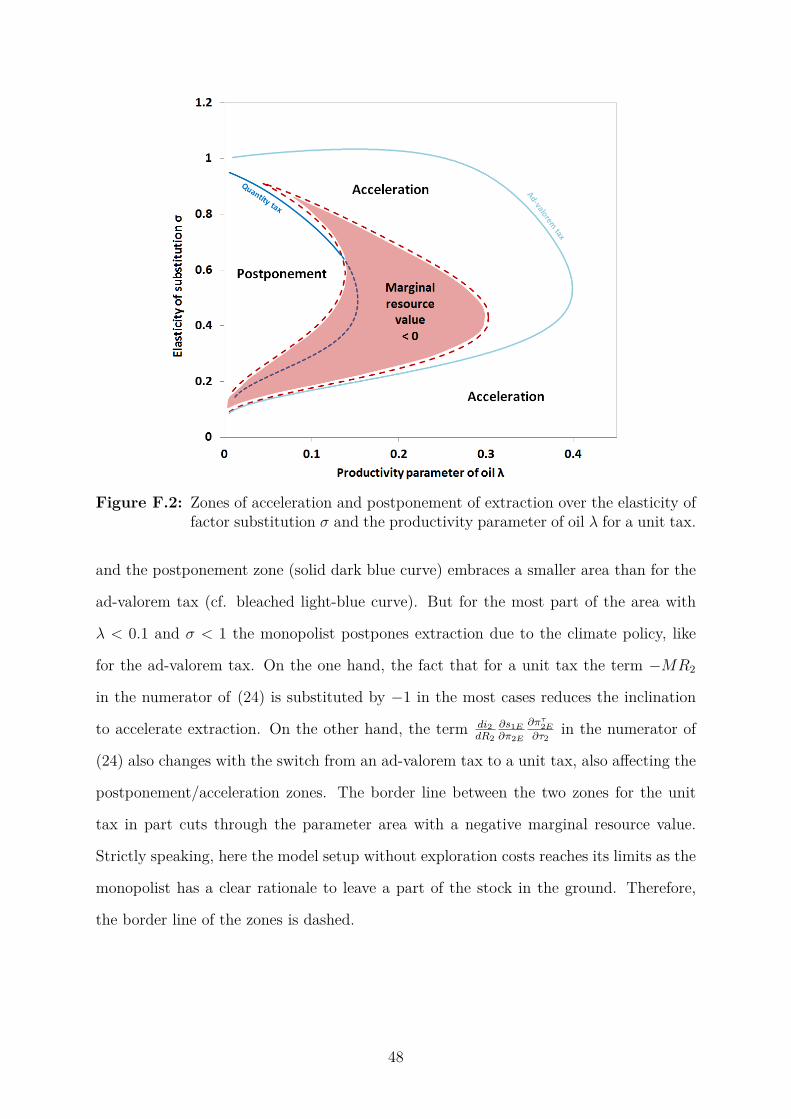
Figure F.2: Zones of acceleration and postponement of extraction over the elasticity offactor substitution σ and the productivity parameter of oil λ for a unit tax.

and the postponement zone (solid dark blue curve) embraces a smaller area than for the

ad-valorem tax (cf. bleached light-blue curve). But for the most part of the area with

λ < 0.1 and σ < 1 the monopolist postpones extraction due to the climate policy, like

for the ad-valorem tax. On the one hand, the fact that for a unit tax the term −MR2

in the numerator of (24) is substituted by −1 in the most cases reduces the inclination

to accelerate extraction. On the other hand, the term di2dR2

∂s1E∂π2E

∂πτ2E∂τ2

in the numerator of

(24) also changes with the switch from an ad-valorem tax to a unit tax, also affecting the

postponement/acceleration zones. The border line between the two zones for the unit

tax in part cuts through the parameter area with a negative marginal resource value.

Strictly speaking, here the model setup without exploration costs reaches its limits as the

monopolist has a clear rationale to leave a part of the stock in the ground. Therefore,

the border line of the zones is dashed.

48

G Sensitivity Analysis for Further Parameters

G.1 Initial Factor Endowments K1 and S̄

The results of the numerical simulation in Figure G.3 show that the initial endowments

of capital and oil can affect the direction of the extraction shift. Obviously, changes

in (relative) factor endowments are closely related to the basic logic of Section 5.1. The

scarcity of oil compared to the other production factors heavily affects the policy reaction

of the extraction path. A higher initial resource endowment leads to a lower marginal

product and to a lower marginal resource revenue (cf. numerator of (24)). The resulting

tax-induced losses in resource rents are lower. This reduces the incentive to accelerate

extraction and makes postponement of extraction more likely (cf. Figure G.3). The same

scarcity reasoning explains the effect of a decrease in capital endowment K1: A lower

initial capital endowment K1 of the world economy decreases the resource’s marginal

revenue and marginal productivity and, thus, makes postponement of extraction more

likely. This suggests that we can expect a different supply-side reaction to a credible

threat of climate policy today than at some other point in the past or the future with

proceeding depletion of the oil stock and capital accumulation over time.

The parameter λ can be seen as a scaling parameter for the marginal revenue of oil

and the according acceleration incentive. This is the reason why changes in both factor

endowments are more pronounced at higher values of the productivity parameter of oil

λ.45

The distribution of initial capital asset endowments can in principle also affect the policy

reaction. If the exporting country’s share in the capital endowment is higher, then its

capital asset motive in the present is reinforced more than the one in the future. The-

refore, present extraction is higher and equilibrium values of all model variables differ.

45 Due to decreasing returns to scale with respect to (K,R), but constant returns to scale with respect to(K,R,L), in final goods production, higher capital endowments can lead to scenarios in which thereis no longer positive capital accumulation as households more and more tend to consume and save outof the given stock, which rises linearly in capital endowments (cf. c1E + c1I +K2 = F1 +K1).

49

Figure G.3: Influence of the initial capital endowment K1 and the resource endowmentS̄ on the borderline between the acceleration and the postponement area(β = 0.3, η = 2, s0E

K1= 0.1).

Unfortunately, if the initial equilibrium before introduction of a climate policy is diffe-

rent, a comparison of reactions to climate policy under various distributions of capital

endowment becomes analytically intractable. The numerical simulation in Figure G.4,

however, shows that a higher share of country E in the (constant) global capital asset

endowment increases the area of extraction postponement. We see that the distribution

of the capital endowment is almost irrelevant for the policy outcome for more realistic

parameter settings of λ < 0.1. But this also implies that transfer payments from the im-

porting to the exporting countries as part of a climate policy agreement would be neither

detrimental, nor beneficial for the result of postponement of oil extraction.

G.2 Household Preferences

The households’ preference parameters β and η also affect the extraction reaction to a

future tax increase. Figure G.5 illustrates the role of the utility discount factor β. A

lower β, indicating higher impatience, reinforces the savings reaction to the tax increase

and the according income loss in the second period ∂s1m∂πτ2m

(cf. (12)). This increases the

50

Figure G.4: Influence of the amount of capital assets of country E s0E on the boundarybetween acceleration and postponement of extraction (β = 0.3, η = 2,K1 = 200, S̄ = 1).

probability of extraction postponement. This effect is more pronounced at higher values

of the productivity parameter of oil λ: The tax-induced income loss and the according

savings adjustment are higher when a higher productivity parameter of oil λ leads to a

higher marginal product and a higher income share of oil.

The second preference parameter η, which indicates the curvature of the utility function

and whose inverse 1ηis the elasticity of intertemporal substitution, also affects the strength

and the sign of the savings reaction to the tax-induced income loss in the future. In

Figure G.6, a higher value of η leads to a stronger future capital asset motive and makes

postponement of extraction more likely in the case of higher substitution elasticites σ.

But the opposite is the case for lower values of σ. The absolute value of the savings

reaction to an income loss ∂s1m∂πτ2m

(cf. (A.1) in the Appendix) is higher for higher values

of η. But the pre-policy equilibrium is different with a different η, as well. This leads

to similar analytical difficulties as in the previous Section G.1. Although the influence

of η depends on other model parameters, the result that extraction is postponed for

reasonable parameter ranges like λ < 0.1 and 0.2 < σ < 0.9 remains rather robust.

51

Figure G.5: Influence of the utility discount factor β on the boundary between accele-ration and postponement of extraction (η = 2, K1 = s0E+s0I = 20+180 =200, S̄ = 1).

Figure G.6: Influence of the elasticity of intertemporal substitution 1ηon the boundary

between acceleration and postponement of extraction (β = 0.3, K1 =s0E + s0I = 20 + 180 = 200, S̄ = 1).

52

References

Abdul-Hamid, Omar, Adedapo Odulaja, Ramadan Janan, Angela Agoawike, and Alvino-

Mario Fantini (2013). OPEC Annual Statistical Bulletin 2013. Vienna. url: https://

www.opec.org/opec_web/static_files_project/media/downloads/publications/

ASB2013.pdf.

Andrade de Sá, Saraly and Julien Daubanes (2016). “Limit pricing and the (in)effectiveness

of the carbon tax”. Journal of Public Economics 139, pp. 28–39.

Anthoff, David, Richard S. J. Tol, and Gary W. Yohe (2009). “Risk aversion, time

preference, and the social cost of carbon”. Environmental Research Letters 4 (2),

p. 24002.

Berk, Istemi and Hakan Yetkiner (2014). “Energy prices and economic growth in the long

run: Theory and evidence”. Renewable and Sustainable Energy Reviews 36, pp. 228–

235.

Bonanno, Giacomo (1990). “Equilibrium theory with imperfect competition”. Journal of

Economic Surveys 4 (4), pp. 297–328.

Central Intelligence Agency (2014). CIA World Factbook. url: https://www.cia.gov/

library/publications/the-world-factbook/.

Cunado, Juncal and Fernando Perez de Gracia (2014). “Oil price shocks and stock market

returns: Evidence for some European countries”. Energy Economics 42, pp. 365–377.

Curuk, Malik and Suphi Sen (2015). “Oil trade and climate policy”. CESifo Working

Paper Series (5285).

Dasgupta, Partha S. and Geoffrey M. Heal (1979). Economic theory and exhaustible

resources. Cambridge Economic Handbooks. Cambridge: Cambridge University Press.

Di Maria, Corrado, Ian Lange, and Edwin van der Werf (2014). “Should we be worried

about the green paradox? Announcement effects of the Acid Rain Program”. European

Economic Review 69, pp. 143–162.

Eichner, Thomas and Rüdiger Pethig (2011). “Carbon leakage, the green paradox, and

perfect future markets”. International Economic Review 52 (3), pp. 767–805.

53

Energy Information Administration (2016a). Online data base - U.S. crude oil composite

acquisition cost by refiners. 2016. url: http://www.eia.gov/dnav/pet/hist/

LeafHandler.ashx?n=PET&s=R0000____3&f=A (visited on 12/02/2016).

Energy Information Administration (2016b). Online data base - U.S. product supplied of

crude oil and petroleum products. 2016. url: http://www.eia.gov/dnav/pet/hist/

LeafHandler.ashx?n=PET&s=MTTUPUS2&f=A (visited on 12/02/2016).

Federal Reserve Bank St. Louis (2016a). Economic data base - Global price of APSP

crude oil. https://fred.stlouisfed.org/series/POILAPSPUSDA. 2016. url: https:

//fred.stlouisfed.org/series/POILAPSPUSDA (visited on 12/02/2016).

Federal Reserve Bank St. Louis (2016b). Economic data base - U.S. gross domestic

product. https://fred.stlouisfed.org/series/FYGDP. 2016. url: https : / / fred .

stlouisfed.org/series/FYGDP (visited on 12/02/2016).

Fouquet, Roger (2014). “Long-run demand for energy services: Income and price elasti-

cities over two hundred years”. Review of Environmental Economics and Policy 8 (2),

pp. 186–207.

Gerlagh, Reyer (2011). “Too Much Oil”. CESifo Economic Studies 57 (1), pp. 79–102.

Grafton, Quentin R., Tom Kompas, and Ngo Van Long (2012). “Substitution between bi-

ofuels and fossil fuels: Is there a green paradox?” Journal of Environmental Economics

and Management 64 (3), pp. 328–341.

Habla, Wolfgang (2016). “The green paradox and interjurisdictional competition across

space and time”. University of Gothenburg Working Papers in Economics (No. 668).

(Visited on 08/08/2016).

Hamilton, James D. (1983). “Oil and the macroeconomy since World War II”. Journal

of Political Economy 91 (2), pp. 228–248.

Hamilton, James D. (2009). “Understanding crude oil prices”. Energy Journal 30 (2),

pp. 179–206.

Hamilton, James D. (2013). “Oil prices, exhaustible resources, and economic growth”.

In: Handbook on Energy and Climate Change. Ed. by Roger Fouquet. Cheltenham,

UK and Northampton, MA, USA: Edward Elgar, pp. 29–57.

54

Hassler, John, Per Krusell, and Conny Olovsson (2010). “Oil monopoly and the climate”.

American Economic Review: Papers & Proceedings 100 (2), pp. 460–464.

Higgins, Matthew, Thomas Klitgaard, and Robert Lerman (2006). “Recycling petrodol-

lars”. Current Issues in Economics and Finance 12 (9).

Hillman, Arye L. and Ngo Van Long (1985). “Monopolistic recycling of oil revenue and

intertemporal bias in oil depletion and trade”. Quarterly Journal of Economics 100 (3),

pp. 597–624.

Jensen, Svenn, Kristina Mohlin, Karen Pittel, and Thomas Sterner (2015). “An intro-

duction to the green paradox: The unintended consequences of climate policies”. Review

of Environmental Economics and Policy 9 (2), pp. 246–265.

Kang, Wensheng, Ronald A. Ratti, and Kyung Hwan Yoon (2014). “The impact of oil

price shocks on U.S. bond market returns”. Energy Economics 44, pp. 248–258.

Kilian, Lutz (2009). “Not all oil price shocks are alike: Disentangling demand and supply

shocks in the crude oil market”. American Economic Review 99 (3), pp. 1053–1069.

Kilian, Lutz and Bruce Hicks (2013). “Did unexpectedly strong economic growth cause

the oil price shock of 2003–2008?” Journal of Forecasting 32 (5), pp. 385–394.

Kilian, Lutz and Daniel P. Murphy (2014). “The role of inventories and speculative

trading in the global market for crude oil”. Journal of Applied Econometrics 29 (3),

pp. 454–478.

Long, Ngo Van (2015). “The green paradox in open economies: Lessons from static and

dynamic models”. Review of Environmental Economics and Policy 9 (2), pp. 266–284.

Long, Ngo Van and Frank Stähler (2016). “General equilibrium effects of green techno-

logical progress”. Environmental and Resource Economics, pp. 1–8.

Marz, Waldemar and Johannes Pfeiffer (2015). “Resource market power and levels of

knowledge in general equilibrium”. IFO Working Paper No. 197.

Moussavian, Mohammed and Larry Samuelson (1984). “On the extraction of an exhausti-

ble resource by a monopoly”. Journal of Environmental Economics and Management

11 (2), pp. 139–146.

55

Nordhaus, William D. (2010). “Economic aspects of global warming in a post-Copenhagen

environment”. Proceedings of the National Academy of Sciences 107 (26), pp. 11721–

11726.

Organisation for Economic Cooperation and Development (2014). World Energy Outlook

2014. Paris: OECD Publishing.

Organisation for Economic Cooperation and Development (2016a). Online data base -

Gross domestic product. 2016. url: https://data.oecd.org/gdp/gross-domestic-

product-gdp.htm (visited on 12/02/2016).

Organisation for Economic Cooperation and Development (2016b). Online data base -

Total oil demand. 2016. url: http://stats.oecd.org/BrandedView.aspx?oecd_

bv_id=oil-data-en&doi=data-00474-en (visited on 12/02/2016).

Organisation for Economic Cooperation and Development and International Labour Or-

ganization (2015). The Labour Share in G20 Economies. Paris. url: https://www.

oecd.org/g20/topics/employment-and-social-policy/The-Labour-Share-in-

G20-Economies.pdf (visited on 11/11/2016).

Sinn, Hans-Werner (2008). “Public policies against global warming: A supply side appro-

ach”. International Tax and Public Finance 15 (4), pp. 360–394.

Smulders, Sjak, Yacov Tsur, and Amos Zemel (2012). “Announcing climate policy: Can

a green paradox arise without scarcity?” Journal of Environmental Economics and

Management 64 (3), pp. 364–376.

Sovereign Wealth Fund Institute (2016). Sovereign Wealth Fund Rankings. url: http:

//www.swfinstitute.org/fund-rankings/ (visited on 08/02/2016).

Stern, David I. and Astrid Kander (2012). “The role of energy in the industrial revolution

and modern economic growth”. Energy Journal 33 (3).

Stiglitz, Joseph (1974). “Growth with exhaustible natural resources: Efficient and optimal

growth paths”. Review of Economic Studies 41, pp. 123–137.

Stiglitz, Joseph E. (1976). “Monopoly and the rate of extraction of exhaustible resources”.

American Economic Review 66 (4), p. 655.

56

Tullock, Gordon (1979). “Monopoly and the rate of extraction of exhaustible resources:

Note”. American Economic Review 69 (1), pp. 231–233.

van der Meijden, Gerard, Frederick van der Ploeg, and Cees Withagen (2015). “Inter-

national capital markets, oil producers and the green paradox”. European Economic

Review 76, pp. 275–297.

van der Ploeg, Frederick (2015). “Second-best carbon taxation in the global economy:

The green paradox and carbon leakage revisited”. CEPR Discussion Paper No. 10549.

van der Ploeg, Frederick and Cees Withagen (2012a). “Is there really a green paradox?”

Journal of Environmental Economics and Management 64 (3) (2012), pp. 342–363.

van der Ploeg, Frederick and Cees Withagen (2012b). “Too much coal, too little oil”.

Journal of Public Economics 96 (1–2) (2012), pp. 62–77.

van der Ploeg, Frederick and Cees Withagen (2015). “Global warming and the green

paradox: A review of adverse effects of climate policies”. Review of Environmental

Economics and Policy 9 (2), pp. 285–303.

van der Werf, Edwin and Corrado Di Maria (2011). “Unintended detrimental effects of

environmental policy: The green paradox and beyond”. CESifo Working Paper Series

(3466).

Waldman, Peter (2016). “Deputy Crown Prince Mohammed bin Salman is preparing

Saudi Arabia for the end of oil”. Bloomberg Businessweek (4/25/2016).

World Bank Group (2016). World DataBank - World Development Indicators. url:

http://databank.worldbank.org/data/reports.aspx?source=2&series=NY.GDP.

PETR.RT.ZS&country=#advancedDownloadOptions (visited on 11/11/2016).

57