iFEM: AN INNOVATIVE FINITE ELEMENT METHOD PACKAGE …

iFEM: AN INNOVATIVE FINITE ELEMENT METHOD PACKAGE IN MATLAB

LONG CHEN

ABSTRACT. Sparse matrixlization, an innovative programming style for MATLAB, is introduced and usedto develop an efficient software package, iFEM, on adaptive finite element methods. In this novel codingstyle, the sparse matrix and its operation is used extensively in the data structure and algorithms. Ourmain algorithms are written in one page long with compact data structure following the style “Ten digit,five seconds, and one page” proposed by Trefethen. The resulting code is simple, readable, and efficient.A unique strength of iFEM is the ability to perform three dimensional local mesh refinement and twodimensional mesh coarsening which are not available in existing MATLAB packages. Numerical examplesindicate that iFEM can solve problems with size 105 unknowns in few seconds in a standard laptop. iFEMcan let researchers considerably reduce development time than traditional programming methods.

1. INTRODUCTION

Finite element method (FEM) is a powerful and popular numerical method on solving partial dif-ferential equations (PDEs), with flexibility in dealing with complex geometric domains and variousboundary conditions. MATLAB (Matrix Laboratory) is a powerful and popular software platform usingmatrix-based script language for scientific and engineering calculations. This paper is on the develop-ment of an finite element method package, with emphasis on adaptive finite element method (AFEM)through local mesh refinement, in MATLAB using an innovative programming style: sparse matrixl-ization. In this novel coding style, to make use of the unique strength of MATLAB on fast matrixoperations, the sparse matrix and its operation is used extensively in the data structure and algorithms.iFEM, the resulting package, is a good balance between simplicity, readability, and efficiency. It willbenefit not only education but also future research and algorithm development on finite element meth-ods.

Finite element methods first decompose the domain into a grid (also indicated by mesh or triangula-tion) consisting of small elements. A family of grids are used to construct appropriate finite dimensionalspaces. Then an appropriate form (so-called weak form) of the original equation is restricted to thosefinite dimensional spaces to get a set of algebraic equations. Solving these algebraic equations will giveapproximated solutions of original PDEs within certain accuracy.

A natural approach to improve the accuracy is to divide each element into small elements which isknown as uniform refinement. However, uniform refinement will dramatically increase the computa-tion effort including the physical memory as well as CPU time since the number of unknowns growsexponentially.

Intuitively only elements in the region where the solution changes dramatically need to be divided.Adaptive finite element method is such a methodology that adjust the element size according to thebehavior of the solution automatically and systematically. Comparing with the uniform refinement,adaptive finite element methods are more preferred to locally increase mesh densities in the regionsof interest, thus saving the computer resources. In this approach, the relation between accuracy andcomputational labor is optimized.

Date: November 15, 2008.2000 Mathematics Subject Classification. 68N15, 65N30, 65M60.Key words and phrases. Matlab program, adaptive Finite Element Method, sparse matrix.The author was supported in part by NSF Grant DMS-0811272, and in part by NIH Grant P50GM76516 and R01GM75309.

1

2 LONG CHEN

Because of its wide application, the finite element method courses are usually offered to engineeringand mathematics students in colleges. Many literature, see, for example, the books [20, 13], are devotedto the theoretical foundation on finite element methods. However, the programming of finite elementmethod is not straightforward. Coding adaptive finite element methods requires sophisticated data struc-ture on the grids and could be very time-consuming. Therefore it is necessary to have a software pack-age with readable implementation of the basic components of adaptive finite element methods. iFEMis such a package implemented in MATLAB. It contains robust, efficient, and easy-following codes forthe main building blocks of adaptive finite element methods.

We choose MATLAB because of its simplicity, readability, and popularity. MATLAB is a high-level programming language. Typically one line MATLAB code can replace ten lines of Fortran orC code. The matrix-based script is expressiveness and very close to the operator-based description ofalgorithms. MATLAB supports a range of operating systems and processor architectures, providingportability and flexibilty. Additionally, MATLAB provides its users with rich graphics capabilities forvisualization. Today MATLAB has emerged as one of the predominant languages of education andtechnical computing.

These merits of using MATLAB in the scientific computing are best summarized in the beautifullittle book “Spectral methods in MATLAB” [60] by Trefethen:

A new era in scientific computing has been ushered in by the development of MATLAB. One can nowpresent advanced numerical algorithms and solutions of nontrivial problems in complete detail withgreat brevity, covering more applied mathematics in a few pages that would have been imaginable a fewyears ago. By sacrificing sometimes (not always!) a certain factor in machine efficiency compared withlower-level languages such as Fortran or C, one obtains with MATLAB a remarkable human efficiency– an ability to modify a program and try something new, then something new again, with unprecedentedease.

All this convenience came at a cost of performance. To be interactive, MATLAB is an interpretlanguage. Indeed a common misperception is “MATLAB is slow for large finite element problems”[22]. This problem is typically due to an incorrect usage of sparse matrix as explained below.

The matrix in the algebraic equation obtained by FEM is a sparse matrix. Namely although theN ×N matrix is of size N2, there are only cN nonzero entries with a small constant c independent ofN . Sparse matrix is the corresponding data structure to take advantage of this sparsity which makes thesimulation of large systems possible. The basic idea of sparse matrix is to use a single array to store allnonzero entries and two additional integer arrays to store the location of nonzero entries.

The accessing and manipulating sparse matrices one element at a time requires searching the indexarrays to find such nonzero entry. It takes time at least proportional to the logarithm of the length ofthe column of the matrix [29]. If the sparse pattern is changed, for example, inserting or removing anonzero, it may require extensive data movement to reform the index and nonzero value arrays. Onthe other hand, since MATLAB is an interpret language, each line is compiled when it is going to beexecuted. If a loop or subroutine caused certain lines to be executed multiple times, they would berecompiled every time.

Therefore manipulating a sparse matrix element-by-element in a large for loop in MATLAB wouldquickly add significant overhead and slow down the performance. Unfortunately the straightforwardimplementation of main components of AFEM typically involves updating sparse matrices in a largeloop over all elements. This is the main reason why most MATLAB implementation of finite elementmethods are slow for number of unknowns larger than thousands.

Therefore the development of an efficient MATLAB package on AFEM is not a simple translationof the code from existing packages using other low-level programming languages. This difference isnot fully noticed in the existing implementation of finite element methods using MATLAB; See, forexample, the books [49, 34, 35] and articles [30, 19, 14, 6, 3, 26, 10, 2]. Codes in some of these workare still written in the low-level fashion. It is simply a translation of other low-level languages, such

iFEM 3

as Fortran or C, to make use of the easy access of MATLAB to public. Some of them aims to shortimplementation of algorithms for the education purpose. In a word, they are simple and readable butnot efficient. 1

We shall gain the efficiency by an innovative programming style: sparse matrixlization. We shallreformulate algorithms on AFEM in terms of matrix operations. To maintain the optimal complexityboth in time and space, we shall use sparse matrix in most places. With such a methodology, wecan make use of fast matrix operations build in the MATLAB. Our numerical examples indicate thatiFEM can solve 2-D problems or 3-D problems with size 105 unknowns in 3 seconds or 8 seconds,respectively, in a standard laptop. Researchers then can easily conduct research and spend less effort onprogramming.

A unique strength of iFEM is the ability to perform three dimensional local mesh refinement andtwo dimensional mesh coarsening which are not available in existing MATLAB packages. Note that thethree dimensional local mesh refinement is not easy to implement due to the complicated geometry andsophisticated data structure. The sparse matrixlization presents an innovative way for the eliminationof hanging nodes and make an efficient implementation of three dimensional local refinement possible.On the coarsening, a unique feature is that only the current mesh instead of the whole refinement historyis required. The algorithm can automatically extract a tree structure from the current grid.

Besides the efficiency, we still maintain the simplicity and readability. In iFEM, our main algorithmsare written in one page long with compact data structure following the style “Ten digit, five seconds,and one page” proposed by Trefethen [61]. User can easily get overview and insight on the algorithmsimplemented, which is impossible to obtain when dealing with closed black-box routines such as thePDEtool box in MATLAB or more advanced commercial package FEMLAB.

We should mention that sparse matrixlization belongs to a more general coding style – vectorization.In the setting of MATLAB programming, vectorization can be understood as a way to replace for loopsby matrix operations or other fast builtin functions. See Code Vectorization Guide at the MathWorksweb page for more tools and techniques on the code vectorization. Sparse matrixlization is a vectoriza-tion technique tailored to adaptive finite element methods. The name sparse matrixlization is used toemphasis the extensive usage of sparse matrix for the data structures and algorithms.

To conclude the introduction, we present the layout of this paper. In Section 2, we shall discussthe data structure of sparse matrices and commands in MATLAB to generate and manipulate sparsematrices. In Section 3, we shall introduce triangulations and discuss efficient ways to construct datastructures for geometric relations using sparse matrixlization. In Section 4, we shall improve the stan-dard but not efficient assembling procedure of stiffness matrix to an efficient way. In Section 5, we shalldiscuss implementation of bisection methods in both two and three dimensions. In Section 6, we shalldiscuss the coarsening of bisection grids in two dimensions. In Section 7, we present a typical loop ofAFEM and present numerical examples using iFEM to illustrate the efficiency of our package. In thelast section, we shall summarize and present future working projects.

2. SPARSE MATRIX IN MATLAB

In this section, we shall explain basics on sparse matrix and corresponding operations in MATLAB,which will be used extensively later. The content presented here is mostly based on Gilbert, Moler andSchereiber [29] and is included here for the convenience of readers.

Sparse matrix is a data structure to take advantage of the sparsity of a matrix. Sparse matrix al-gorithms require less computational time by avoiding operations on zero entries and sparse matrix datastructures require less computer memory by not storing many zero entries. We refer to books [44, 25, 23]for detailed description on sparse matrix data structure and [54] for a quick introduction on popular data

1Very recently Funken, Praetorius, and Wissgott [28] provide an efficient implementation of adaptive P1 finite element methodin two dimensions in MATLAB. Our package is developed independently and includes adaptive finite element in three dimensionswhich is much harder than that in two dimensions.

4 LONG CHEN

structures of sparse matrix. In particular, the sparse matrix data structure and operations has been addedto MATLAB by Gilbert, Moler and Schereiber and documented in [29].

2.1. Storage scheme. There are different types of data structures for the sparse matrix. All of themshare the same basic idea: use a single array to store all nonzero entries and two additional integer arraysto store the indices of nonzero entries.

A natural scheme, known as coordinate format, is to store both the row and column indices. In thesequel, we suppose A is a m × n matrix containing only nnz nonzero elements. Let us look at thefollowing simple example:

(1) A =

1 0 00 2 40 0 00 9 0

, i =

1242

, j =

1223

, s =

1294

.In this example, i vector stores row indices of non-zeros, j column indices, and s the value of non-zeros. All three vectors have the same length nnz. The two indices vectors i and j contains redundantinformation. We can compress the column index vector j to a column pointer vector with length n+ 1.The value j(k) is the pointer to the beginning of k-th column in the vector of i and s, and j(n + 1) =nnz+ 1. This scheme is known as Compressed Sparse Column (CSC) scheme and is used in MATLABsparse matrices package. For example, in CSC formate, the vector to store the column pointer will bej = [ 1 2 4 5 ]t. Comparing with coordinate formate, CSC formate saves storage for nnz − n − 1integers which could be nonnegligilble when the number of nonzero is much larger than that of thecolumn. In CSC formate it is efficient to extract a column of a sparse matrix. For example, the k-thcolumn of a sparse matrix can be build from the index vector i and the value vector s ranging from j(k)to j(k+ 1)− 1. There is no need of searching index arrays. An algorithm that builds up a sparse matrixone column at a time can be also implemented efficiently [29].

Remark 2.1. CSC is an internal representation of sparse matrices in MATLAB. For user convenience,the coordinate scheme is presented as the interface. This allows users to create and decompose sparsematrices in a more straightforward way.

Comparing with the dense matrix, the sparse matrix lost the direct relation between the index (i,j)and the physical location to save the value A(i,j). The accessing and manipulating matrices oneelement at a time requires the searching of the index vectors to find such nonzero entry. It takes timeat least proportional to the logarithm of the length of the column; inserting or removing a nonzeromay require extensive data movement [29]. Therefore, do not manipulate a sparse matrix element-by-element in a for loop in MATLAB.

Due to the lost of the link between the index and the value of entries, the operations on sparsematrices is delicate. One needs to write subroutines for standard matrix operations: multiplication of amatrix and a vector, addition of two sparse matrices, and transpose of sparse matrices etc. Since someoperations will change the sparse pattern, typically there is a priori loop to set up the nonzero pattern ofthe resulting sparse matrix. Good sparse matrix algorithms should follow the “time is proportional toflops” rule [29]: The time required for a sparse matrix operation should be proportional to the numberof arithmetic operations on nonzero quantities. The sparse package in MATLAB follows this rule; See[29] for details.

2.2. Create and decompose sparse matrix. To create a sparse matrix, we first form i, j and s vectors,i.e., a list of nonzero entries and their indices, and then call the function sparse using i, j, s as input.Several alternative forms of sparse (with more than one argument) allow this. The most commonlyused one is

A = sparse(i,j,s,m,n).

iFEM 5

This call generates an m × n sparse matrix, using [i, j, s] as the coordinate formate. The first threearguments all have the same length. However, the indices in these three vectors need not be given inany particular order and could have duplications. If a pair of indices occurs more than once in i and j,sparse adds the corresponding values of s together. This nice summation property is very useful forfinite element computation.

The function [i,j,s]=find(A) is the inverse of sparse function. It will extract the nonzeroelements together with their indices. The indices set (i, j) are sorted in column major order and thus thenonzero A(i,j) is sorted in lexicographic order of (j,i) not (i,j). See the example in (1).

Remark 2.2. There is a similar command accumarray to create a dense matrix A from indices andvalues. It is slightly different from sparse. We need to pair [i j] to form a subscript vector. So is thedimension [m n]. Since the accessing of a single element in a dense matrix is much faster than that ina sparse matrix, when m or n is small, say n = 1, it is better to use accumarray instead of sparse. Amost commonly used command is

accumarray([i j], s, [m n]).

3. TRIANGULATION

In this section, we shall discuss triangulations used in finite element methods. We would like todistinguish two structures of a triangulation: one is the topology of a mesh which is determined by thecombinatorial connectivity of vertices; another is the geometric shape which depends on the location ofvertices. Correspondingly there are two basic data structure used to represents a triangulation. The datastructures and corresponding algorithms on the topological/combinatorial structure of triangulationsdiscussed here can be applied to other adaptive methods or other discretization methods. Note that thetopological/combinatorial structure of triangulations is not thoroughly discussed in the literature.

3.1. Geometric simplex and triangulation. Let xi = (x1,i, · · · , xd,i)t, i = 1, · · · , d + 1, be d + 1points in Rd, d ≥ 1, which do not all lie in one hyper-plane. The convex hull of the d + 1 pointsx1, · · · ,xd+1,

(2) τ := x =d+1∑i=1

λixi | 0 ≤ λi ≤ 1, i = 1 : d+ 1,d+1∑i=1

λi = 1

is defined as a geometric d-simplex generated (or spanned) by the vertices x1, · · · ,xd+1. For example,a triangle is a 2-simplex and a tetrahedron is a 3-simplex. For the convenience of notation, we also call apoint 0-simplex. For an integer 0 ≤ m ≤ d−1, anm-dimensional face of τ is anym-simplex generatedby m+ 1 of the vertices of τ . Zero-dimenisonal faces are called vertices or nodes and one-dimensionalfaces are called edges.

The numbers λ1(x), · · · , λd+1(x) are called barycentric coordinates of x with respect to the d+ 1points x1, · · · ,xd+1. There is a simple geometric meaning of the barycentric coordinates. Given ax ∈ τ , let τi(x) be the simplex by replacing the vertex xi of τ by x. Then it can be shown that

(3) λi(x) = |τi(x)|/|τ |,where | · | is the Lebesgure measure in Rd, namely area in two dimensions and volume in three dimen-sions. From (3), it is easy to deduce that λi(x) is an affine function of x and vanished on the (d−1)-faceopposite to the vertex xi.

Let Ω be a polyhedral domain in Rd, d ≥ 1. A geometric triangulation T of Ω is a set of d-simplicessuch that

∪τ∈T τ = Ω, andτi ∩ τj= ∅, for any τi, τj ∈ T , i 6= j.

Remark 3.1. There are other type of meshes by partition the domain into quadrilateral (in 2-D), cube(in 3-D), hexahedron (in 3-D), and so on. In this paper, we restrict ourself to simplicial triangulations

6 LONG CHEN

and thus will mix the usage of three words: grid, triangulation, and mesh. We also identify the words‘node’ and ‘vertex’ since only linear element will be used in this paper.

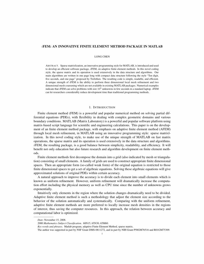
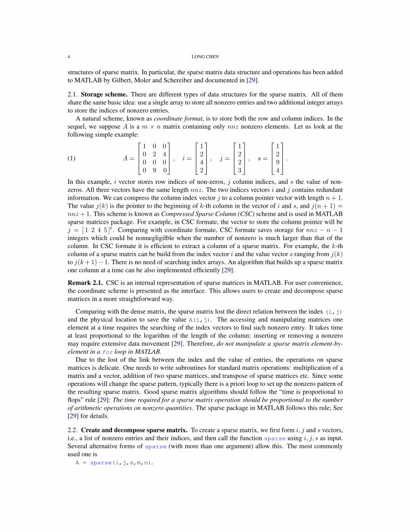
There are two conditions that we shall impose on triangulations that are important in the finite ele-ment computation. The first requirement is a topological property. A triangulation T is called conform-ing or compatible if the intersection of any two simplexes τ and τ ′ in T is either empty or a commonlower dimensional simplex (nodes in two dimensions, nodes and edges in three dimensions). The nodefalls into the interior of a simplex is called a hanging node; See Figure 1 (a).

(a) Bisect a triangle (b) Completion

FIGURE 1. Newest vertex bisection

1

(a) A triangulation with a hanging node(a) Bisect a triangle (b) Completion

FIGURE 1. Newest vertex bisection

1

(b) A conforming triangulation

FIGURE 1. Two triangulations. The left is non-conforming and the right is conforming.

The second important condition is on the geometric structure. A set of triangulations T is calledshape regular if there exists a constant c0 such that

(4) maxτ∈T

diam(τ)d

|τ | ≤ c0, ∀ T ∈ T ,

where diam(τ) is the diameter of τ . In two dimensions, it is equivalent to the minimal angle of eachtriangulation is bounded below uniformly in the shape regular class.

Remark 3.2. In addition to (4), if there exists a constant c1 such that

(5)maxτ∈T |τ |minτ∈T |τ | ≤ c1, ∀ T ∈ T ,

T is called quasi-uniform.

3.2. Abstract simplex and simplicial complex. To distinguish the topological structure with geomet-ric one, we now understand the points as abstract entities and introduce abstract simplex or combinato-rial simplex [48]. The set τ = v1, · · · , vd+1 of d + 1 abstract points is called an abstract d-simplex.A face σ of a simplex τ is a simplex determined by a non-empty subset of τ . A proper face is any facedifferent from τ .

Let N = v1, v2, · · · , vN be a set of N abstract points. An abstract/combinatorial simplicialcomplex T is a set of simplices formed by finite subsets of N such that

(1) if τ ∈ T is a simplex, then any face of τ is also a simplex in T ;(2) for two simplices τ1, τ2 ∈ T , the intersection τ1 ∩ τ2 is a face of both τ1 and τ2.

By the definition, a two dimensional combinatorial simplicial complex T contains not only trianglesbut also edges and vertices of these triangles. A geometric triangulation defined before is only a set ofd-simplex but no faces. By including all faces, we shall get a simplicial complex if the triangulation isconforming which corresponds to the second requirement of a simplicial simplex.

A subset M ⊂ T is a subcomplex of T if M is a simplicial complex itself. Important classes ofsubcomplex includes the star or ring of a simplex. That is for a simplex σ ∈ T

star(σ) = τ ∈ T , σ ⊂ τ.If two, or more, simplices of T share a common face, they are called adjacent or neighbors. The

boundary of T is formed by any proper face that belongs to only one simplex, and its faces.

iFEM 7

By associating the set of abstract points with geometric points in Rn, n ≥ d, we obtain a geometricshape consisting of piecewise flat simplices. This is called a geometric realization of an abstract sim-plicial complex or, using the terminology of geometry, the embedding of T into Rn. The embedding isuniquely determined by the identification of abstract and geometric vertices.

A planar triangulation is a two dimensional abstract simplicial complex which can be embeddedinto R2 and thus called 2-D triangulation. A 2-D simplicial complex could also be embedding intoR3 and result a triangulation of a surface. Therefore the surface mesh in R3 is usually called 2 1

2 -Dtriangulation. For these two different embedding, they many have the same combinatorary structure asan abstract simplicial complex but different geometric structure by representing a flat domain in R2 ora surface in R3.

3.3. Data structure for triangulations. We shall discuss the data structure to represent triangulationsand facilitate the mesh adaptation procedure. There is a dilemma for the data structure in the imple-mentation level. If more sophisticated data structure is used to easily traverse in the mesh, for example,to save the star of vertices or edges, it will simplify the implementation of most adaptive finite elementsubroutines. On the other hand, if the triangulation is changed, for example, a triangle is bisected, onehas to update those data structure which in turn complicates the implementation.

Our solution is to maintain two basic data structure and construct auxiliary data structure inside eachsubroutine when it is necessary. It is not optimal in terms of the computational cost. But it will benefitthe interface of accessing subroutines, simplify the coding and save the memory. Also as we shall seesoon, the auxiliary data structure can be constructed by sparse matrixlization efficiently. This is anexample we scarifies a small factor of efficiency to gain the simplicity.

3.3.1. Basic data structure. The matrices node(1:N,1:d) and elem(1:NT,1:d+1) are used to rep-resent a d-dimensional triangulation embedded in Rd, where N is the number of vertices and NT is thenumber of elements. These two matrices represent two different structure of a triangulation: elem forthe topology and node for the embedding.

The matrix elem represents a set of abstract simplices. The index set 1, 2, · · · , N is called theglobal index set of vertices. Here a vertex is thought as an abstract entity. By definition, elem(t,1:d+1)are the global indices of d+ 1 vertices which form the abstract d-simplex t. Note that any permutationof vertices of t will represent the same abstract simplex.

The matrix node gives the geometric realization of the simplicial complex. For example, for a 2-Dtriangulation, node(k,1:2) contain x- and y-coordinates of the k-th node. We shall always order thevertices of a simplex such that the signed volume is positive. That is in 2-D, three vertices of a triangleis ordered counter-clockwise and in 3-D, the ordering of vertices follows the right-hand rule. Note thateven permutation of vertices is still allowed to represent the same element.

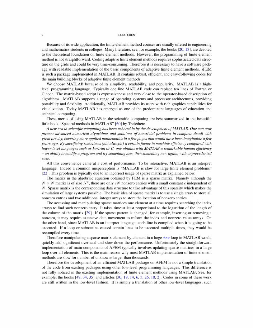
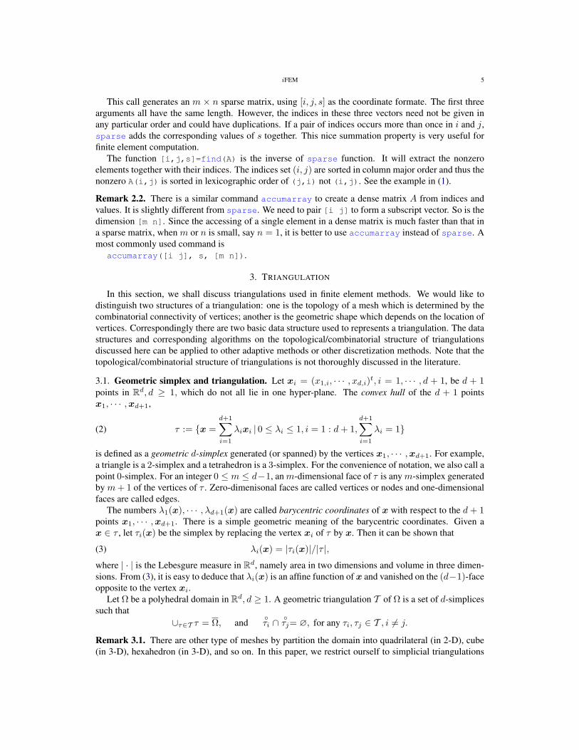
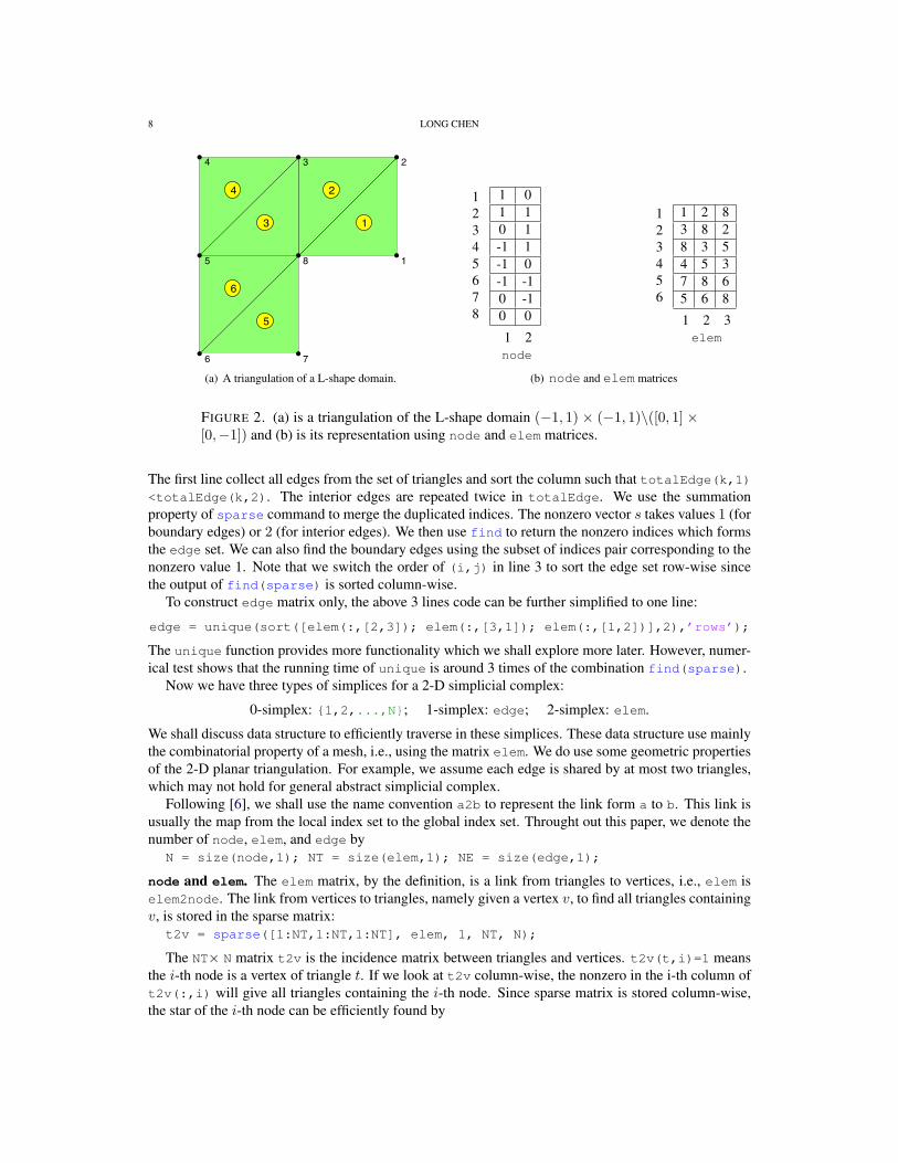
As an example, node and elem matrices to represent the triangulation of the L-shape domain(−1, 1)× (−1, 1)\([0, 1]× [0,−1]) in the Figure 2 (a) and (b).

3.3.2. Auxiliary data structure for 2-D triangulation. We shall discuss how to extract the topologicalor combinatorial structure of a triangulation by using elem array only. The combinatorial structure willbenefit the implementation of finite element methods.

edge. We first complete the 2-D simplicial complex by constructing the 1-dimensional simplex. In thematrix edge(1:NE,1:2), the first and second rows contain indices of the starting and ending points.The column is sorted in the way that for the k-th edge, edge(k,1)<edge(k,2). The following codewill generate an edge matrix.

1 totalEdge = sort([elem(:,[2,3]); elem(:,[3,1]); elem(:,[1,2])],2);

2 [i,j,s] = find(sparse(totalEdge(:,2),totalEdge(:,1),1));

3 edge = [j,i]; bdEdge = [j(s==1),i(s==1)];

8 LONG CHEN

1

234

5

6 7

8

1

2

3

4

5

6

(a) A triangulation of a L-shape domain.

8 LONG CHEN

1

234

5

6 7

8

1

2

3

4

5

6

FIGURE 3. A triangulation of a L-shape domain.

12345678

1 01 10 1-1 1-1 0-1 -10 -10 0

1 2node

123456

1 2 83 8 28 3 54 5 37 8 65 6 8

1 2 3elem

123456789

10111213

1 21 82 32 83 43 53 84 55 65 86 76 87 8

1 2edge

TABLE 1. node,elem and edge matrices for the L-shape domain in Figure 3.

3.3.2. Auxiliary data structure for 2-D triangulation. We shall discuss how to extract the topologicalor combinatorial structure of a triangulation by using elem array only. The combinatorial structure willbenefit the finite element implementation.

edge. We first complete the 2-D simplicial complex by constructing the 1-dimensional simplex. In thematrix edge(1:NE,1:2), the first and second rows contain indices of the starting and ending points.The column is sorted in the way that for the k-th edge, edge(k,1)<edge(k,2). The following codewill generate an edge matrix.



3 edge = [j,i]; bdEdge = [j(s==1),i(s==1)];

The first line collect all edges from the set of triangles and sort the column such that totalEdge(k,1)<totalEdge(k,2). The interior edges are repeated twice in totalEdge. We use the summationproperty of sparse command to merge the duplicated indices. The nonzero vector s takes values 1 (forboundary edges) or 2 (for interior edges). We then use find to return the nonzero indices which forms

(b) node and elem matrices

FIGURE 2. (a) is a triangulation of the L-shape domain (−1, 1) × (−1, 1)\([0, 1] ×[0,−1]) and (b) is its representation using node and elem matrices.

The first line collect all edges from the set of triangles and sort the column such that totalEdge(k,1)<totalEdge(k,2). The interior edges are repeated twice in totalEdge. We use the summationproperty of sparse command to merge the duplicated indices. The nonzero vector s takes values 1 (forboundary edges) or 2 (for interior edges). We then use find to return the nonzero indices which formsthe edge set. We can also find the boundary edges using the subset of indices pair corresponding to thenonzero value 1. Note that we switch the order of (i,j) in line 3 to sort the edge set row-wise sincethe output of find(sparse) is sorted column-wise.

To construct edge matrix only, the above 3 lines code can be further simplified to one line:

edge = unique(sort([elem(:,[2,3]); elem(:,[3,1]); elem(:,[1,2])],2),’rows’);

The unique function provides more functionality which we shall explore more later. However, numer-ical test shows that the running time of unique is around 3 times of the combination find(sparse).

Now we have three types of simplices for a 2-D simplicial complex:

0-simplex: 1,2,...,N; 1-simplex: edge; 2-simplex: elem.

We shall discuss data structure to efficiently traverse in these simplices. These data structure use mainlythe combinatorial property of a mesh, i.e., using the matrix elem. We do use some geometric propertiesof the 2-D planar triangulation. For example, we assume each edge is shared by at most two triangles,which may not hold for general abstract simplicial complex.

Following [6], we shall use the name convention a2b to represent the link form a to b. This link isusually the map from the local index set to the global index set. Throught out this paper, we denote thenumber of node, elem, and edge by

N = size(node,1); NT = size(elem,1); NE = size(edge,1);

node and elem. The elem matrix, by the definition, is a link from triangles to vertices, i.e., elem iselem2node. The link from vertices to triangles, namely given a vertex v, to find all triangles containingv, is stored in the sparse matrix:

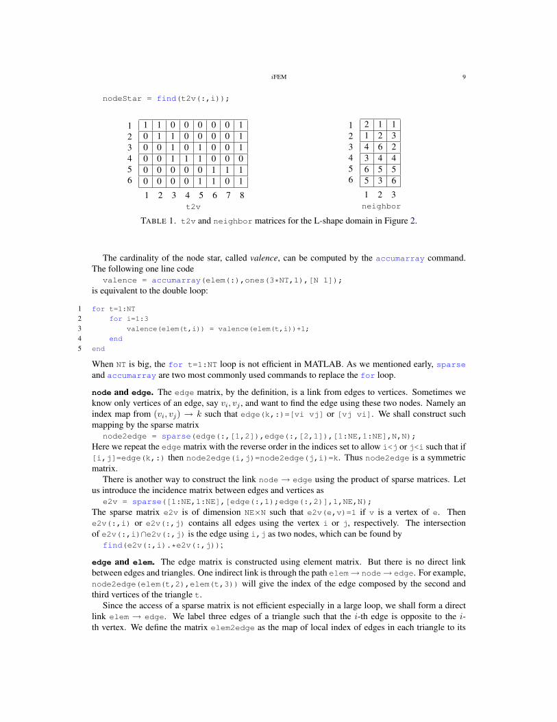
t2v = sparse([1:NT,1:NT,1:NT], elem, 1, NT, N);

The NT× N matrix t2v is the incidence matrix between triangles and vertices. t2v(t,i)=1 meansthe i-th node is a vertex of triangle t. If we look at t2v column-wise, the nonzero in the i-th column oft2v(:,i) will give all triangles containing the i-th node. Since sparse matrix is stored column-wise,the star of the i-th node can be efficiently found by

iFEM 9

nodeStar = find(t2v(:,i));

123456

1 1 0 0 0 0 0 10 1 1 0 0 0 0 10 0 1 0 1 0 0 10 0 1 1 1 0 0 00 0 0 0 0 1 1 10 0 0 0 1 1 0 1

1 2 3 4 5 6 7 8t2v

123456

2 1 11 2 34 6 23 4 46 5 55 3 6

1 2 3neighbor

TABLE 1. t2v and neighbor matrices for the L-shape domain in Figure 2.

The cardinality of the node star, called valence, can be computed by the accumarray command.The following one line code

valence = accumarray(elem(:),ones(3*NT,1),[N 1]);

is equivalent to the double loop:

1 for t=1:NT

2 for i=1:3

3 valence(elem(t,i)) = valence(elem(t,i))+1;

4 end

5 end

When NT is big, the for t=1:NT loop is not efficient in MATLAB. As we mentioned early, sparseand accumarray are two most commonly used commands to replace the for loop.

node and edge. The edge matrix, by the definition, is a link from edges to vertices. Sometimes weknow only vertices of an edge, say vi, vj , and want to find the edge using these two nodes. Namely anindex map from (vi, vj) → k such that edge(k,:)=[vi vj] or [vj vi]. We shall construct suchmapping by the sparse matrix

node2edge = sparse(edge(:,[1,2]),edge(:,[2,1]),[1:NE,1:NE],N,N);

Here we repeat the edge matrix with the reverse order in the indices set to allow i<j or j<i such that if[i,j]=edge(k,:) then node2edge(i,j)=node2edge(j,i)=k. Thus node2edge is a symmetricmatrix.

There is another way to construct the link node→ edge using the product of sparse matrices. Letus introduce the incidence matrix between edges and vertices as

e2v = sparse([1:NE,1:NE],[edge(:,1);edge(:,2)],1,NE,N);

The sparse matrix e2v is of dimension NE×N such that e2v(e,v)=1 if v is a vertex of e. Thene2v(:,i) or e2v(:,j) contains all edges using the vertex i or j, respectively. The intersectionof e2v(:,i)∩e2v(:,j) is the edge using i,j as two nodes, which can be found by

find(e2v(:,i).*e2v(:,j));

edge and elem. The edge matrix is constructed using element matrix. But there is no direct linkbetween edges and triangles. One indirect link is through the path elem→ node→ edge. For example,node2edge(elem(t,2),elem(t,3)) will give the index of the edge composed by the second andthird vertices of the triangle t.

Since the access of a sparse matrix is not efficient especially in a large loop, we shall form a directlink elem → edge. We label three edges of a triangle such that the i-th edge is opposite to the i-th vertex. We define the matrix elem2edge as the map of local index of edges in each triangle to its

10 LONG CHEN

global index. The following three lines code will construct elem2edge using more output from unique

function.


2 [edge, i2, j] = unique(totalEdge,’rows’);

3 elem2edge = reshape(j,NT,3);

Line 1 collects all edges element-wise. The size of totalEdge is thus 3NT×2. By the construction,there is a natural index mapping from totalEdge to elem. In line 2, we apply unique function toobtain the edge matrix. The output index vectors i2 and j contain the index mapping between edge

and totalEdge. Here i2 is a NE×1 vector to index the last (2-nd in our case) occurrence of eachunique value in totalEdge such that edge = totalEdge(i2,:), while j is a 3NT×1 vector suchthat totalEdge = edge(j,:). (Try help unique in MATLAB to learn more examples.) Thenusing the natural index mapping from totalEdge to elem, we reshape the 3NT×1 vector j to a NT×3matrix which is elem2edge.

An alternative but more cost way to construct elem2edge using the product of sparse matrices willbe discussed for 3-D mesh.

We then define a NE×4 matrix edge2elem such that edge2elem(k,1) and edge2elem(k,2)

are two triangles sharing the k-th edge for an interior edge. If the k-th edge is on the boundary,then we set edge2elem(k,1) = edge2elem(k,2). Furthermore, we shall record the local indicesin edge2elem(k,3:4) such that elem2edge(edge2elem(k,1),edge2elem(k,3))=k. Similarlyedge2elem(k,4) is the local index of k-th edge in edge2elem(k,2).

To construct edge2elem matrix, we need to find out the index map from edge to elem. The follow-ing code is a continuation of the code constructing elem2edge.

1 i1(j(3*NT:-1:1)) = 3*NT:-1:1; i1=i1’;

2 k1 = ceil(i1/NT); t1 = i1 - NT*(k1-1);

3 k2 = ceil(i2/NT); t2 = i2 - NT*(k2-1);

4 edge2elem = [t1,t2,k1,k2];

The code in line 1 use j to find the first occurrence of each unique edge in the totalEdge. In MATLAB,when assign values using an index vector with duplication, the value at the repeated index will bethe last one assigned to this location. Obvious j contains duplication of edge indices. For example,j(1)=j(2)=4which means totalEdge(1,:)=totalEdge(2,:)=edge(4,:). We reverse the orderof j such that i1(4)=1 which is the first occurrence.

Using the natural index mapping from totalEdge to elem, for an index i between 1:N, the formulak=ceil(i/NT) computes the local index of i-th edge, and t=i-NT*(k-1) is the global index of thetriangle which totalEdge(i,:) belongs to. The edge2elem is just composed by t1,t2,k1 and k2.

elem and elem. We use the matrix neighbor(1:NT,1:3) to record the neighboring triangles foreach triangle. By definition, neighbor(t,i) is opposite to the i-th vertex of the t-th triangle. If iis opposite to the boundary, then we set neighbor(t,i)=t. Using the index map between edge andelem, we can easily form the neighbor matrix by the following 2 lines code.

1 ix = (i1 ˜= i2);

2 neighbor = accumarray([[t1(ix),k1(ix)];[t2,k2]],[t2(ix);t1],[NT 3]);

In line 1, to avoid the duplication in the index array, we find the index set of interior edges by notingthat if e is a boundary edge, then i1(e)=i2(e). Since t1 and t2 share the same edge, we form theneighbor matrix by using t1,k1 and t2,k2 as indices set and t2,t1 as the value in line 2.

We summarize the construction of these auxiliary data structure in a subroutine auxstructure.m.

1 function [neighbor,elem2edge,edge2elem,edge,bdEdge]=auxstructure(elem)


iFEM 11

3 [edge, i2, j] = unique(totalEdge,’rows’);

4 NT = size(elem,1);

5 elem2edge = reshape(j,NT,3);

6 i1(j(3*NT:-1:1)) = 3*NT:-1:1; i1=i1’;

7 k1 = ceil(i1/NT); t1 = i1 - NT*(k1-1);

8 k2 = ceil(i2/NT); t2 = i2 - NT*(k2-1);

9 ix = (i1 ˜= i2);


11 bdEdge = edge((i1 == i2),:);

12 edge2elem = [t1,t2,k1,k2];

3.3.3. Auxiliary data structure for 3-D triangulation. Most codes discussed for 2-D triangulations canbe generalized to 3-D triangulations in a straightforward way. Due to the page limit, we pick up thefollowing important data structures to explain in detail.

elem and face. The face matrix, which represents the 2-D simplex, can be generated by the uniquefunction of all element-wise faces. The link elem2face, faceStar, and neighbor can be constructedsimilarly using the index map. We list auxstructure3.m below and skip the explanation.

1 function [neighbor,elem2face,face2elem,face,bdFace] = auxstructure3(elem)

2 face = [elem(:,[2 4 3]);elem(:,[1 3 4]);elem(:, [1 4 2]);elem(:, [1 2 3])];

3 [face, i2, j] = unique(sort(face,2),’rows’);

4 NT = size(elem,1);

5 elem2face = reshape(j,NT,4);

6 i1(j(4*NT:-1:1)) = 4*NT:-1:1; i1 = i1’;

7 k1 = ceil(i1/NT); t1 = i1 - NT*(k1-1);

8 k2 = ceil(i2/NT); t2 = i2 - NT*(k2-1);

9 ix = (i1 ˜= i2);


11 bdFace = face((i1 == i2),:);

12 face2elem = [t1,t2,k1,k2];

elem and edge. The edge matrix can be generated using find(sparse) commands as in the 2-Dcase. The vector edgeValence is used to denote the number of elements sharing each edge.

1 totalEdge = sort([elem(t,[1 2]); elem(t,[1 3]); elem(t,[1 4]); ...

2 elem(t,[2 3]); elem(t,[2 4]); elem(t,[3 4])],2);


4 edge = [j,i]; edgeValence = s;

We then find the link elem2edge which is useful for the high order elements and edge element.

1 e2v = sparse([1:NE,1:NE],[edge(:,1);edge(:,2)],1,NE,N);

2 [i,j,s] = find(e2v(:,totalEdge(:,1)).*e2v(:,totalEdge(:,2)));

3 elem2edge = reshape(i,NT,6);

The first line generates the incidence matrix between edges and vertices. The sparse matrix e2v is ofdimension NE×N such that e2v(e,v)=1 if v is a vertex of e. Then e2v(:,p1) or e2v(:,p2) containsall edges using the vertex p1 or p2, respectively. The intersection of e2v(:,p1)∩e2v(:,p2) is theedge using p1 and p2 as two vertices. The intersection is found by the Hadamard product, i.e., itemwise product, of two sparse matrices e2v(:,totalEdge(:,1)) and e2v(:,totalEdge(:,2)), andrecorded in the index set i. In line 3 the 6NT×1 vector i is reshaped to a NT×6 matrix which is whatwe want.

We now discuss the construction of edgeStar. This link from edge to elem is important since the3-D local mesh refinement is always cutting edges. Unlike the 2-D case, we cannot use a NE×2 dense

12 LONG CHEN

matrix for edgeStar since the number of elements sharing one edge varies a lot. Again we shall resortto the sparse matrix.

1 t2v = sparse([1:NT,1:NT,1:NT,1:NT], elem(1:NT,:), 1, NT, N);

2 nodeStar1 = t2v(1:NT,edge(:,1));

3 nodeStar2 = t2v(1:NT,edge(:,2));

4 edgeStar = nodeStar1.*nodeStar2;

The elements containing an edge is characterized as the intersection two stars of the ending nodes ofthis edge. The first line generates the incidence matrix t2v. Line 2 and 3 extract columns from t2v.The intersection is found by the Hadamard product of two sparse matrix nodeStar1 and nodeStar2.The resulting sparse matrix edgeStar is a NT×NE sparse matrix and find(edgeStar(:,i)) will givethe element indices containing the i-th edge.

In the construction of elem2edge and edgeStar, we use Hadamard product of sparse matrices tofind the quantity associated two index sets. This technique is crucial in 3-D refinement.

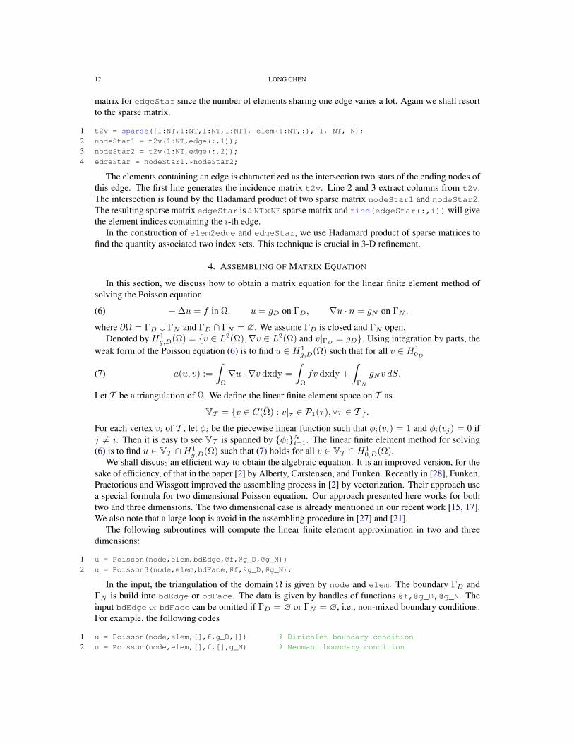
4. ASSEMBLING OF MATRIX EQUATION

In this section, we discuss how to obtain a matrix equation for the linear finite element method ofsolving the Poisson equation

(6) −∆u = f in Ω, u = gD on ΓD, ∇u · n = gN on ΓN ,

where ∂Ω = ΓD ∪ ΓN and ΓD ∩ ΓN = ∅. We assume ΓD is closed and ΓN open.Denoted by H1

g,D(Ω) = v ∈ L2(Ω),∇v ∈ L2(Ω) and v|ΓD= gD. Using integration by parts, the

weak form of the Poisson equation (6) is to find u ∈ H1g,D(Ω) such that for all v ∈ H1

0D

(7) a(u, v) :=∫

Ω

∇u · ∇v dxdy =∫

Ω

fv dxdy +∫

ΓN

gNv dS.

Let T be a triangulation of Ω. We define the linear finite element space on T as

VT = v ∈ C(Ω) : v|τ ∈ P1(τ),∀τ ∈ T .For each vertex vi of T , let φi be the piecewise linear function such that φi(vi) = 1 and φi(vj) = 0 ifj 6= i. Then it is easy to see VT is spanned by φiNi=1. The linear finite element method for solving(6) is to find u ∈ VT ∩H1

g,D(Ω) such that (7) holds for all v ∈ VT ∩H10,D(Ω).

We shall discuss an efficient way to obtain the algebraic equation. It is an improved version, for thesake of efficiency, of that in the paper [2] by Alberty, Carstensen, and Funken. Recently in [28], Funken,Praetorious and Wissgott improved the assembling process in [2] by vectorization. Their approach usea special formula for two dimensional Poisson equation. Our approach presented here works for bothtwo and three dimensions. The two dimensional case is already mentioned in our recent work [15, 17].We also note that a large loop is avoid in the assembling procedure in [27] and [21].

The following subroutines will compute the linear finite element approximation in two and threedimensions:

1 u = Poisson(node,elem,bdEdge,@f,@g_D,@g_N);

2 u = Poisson3(node,elem,bdFace,@f,@g_D,@g_N);

In the input, the triangulation of the domain Ω is given by node and elem. The boundary ΓD andΓN is build into bdEdge or bdFace. The data is given by handles of functions @f,@g_D,@g_N. Theinput bdEdge or bdFace can be omitted if ΓD = ∅ or ΓN = ∅, i.e., non-mixed boundary conditions.For example, the following codes

1 u = Poisson(node,elem,[],f,g_D,[]) % Dirichlet boundary condition

2 u = Poisson(node,elem,[],f,[],g_N) % Neumann boundary condition

iFEM 13

will compute the solution to the Poisson equation with Dirichlet or Neumann boundary condition in thewhole boundary ∂Ω. The boundary will be found by find(sparse) commands. See also Section 4.3.This provides more flexibility in mesh adaptation without tracking boundary edges or faces.

4.1. Assembling the stiffness matrix. For any function v ∈ VT , there is a unique representation:v =

∑Ni=1 viφi. We define an isomorphism VT ∼= RN by

(8) v =N∑i=1

viφi ←→ v = (v1, · · · , vN )t,

and call v the vector representation of v (with respect to the basis φiNi=1). We introduce the stiffnessmatrix

A = (aij)N×N , with aij = a(φj , φi).In this subsection, we shall discuss how to form the matrixA efficiently in MATLAB.

4.1.1. Standard assembling process. By the definition, for 1 ≤ i, j ≤ N ,

aij =∫

Ω

∇φj · ∇φi dx =∑τ∈T

∫τ

∇φj · ∇φi dx.

For each simplex τ , we define the local stiffness matrix Aτ = (aτij)(d+1)×(d+1) as

aτij =∫τ

∇λj · ∇λi dx, for 1 ≤ i, j ≤ d+ 1.

The computation of aij will be decomposed into the computation of local stiffness matrix, aτij and thesummation over all elements. Note that the index set in aτij is local index while in aij it is global index.The assembling process is to distribute the quantity associated to the local index to that to the globalindex.

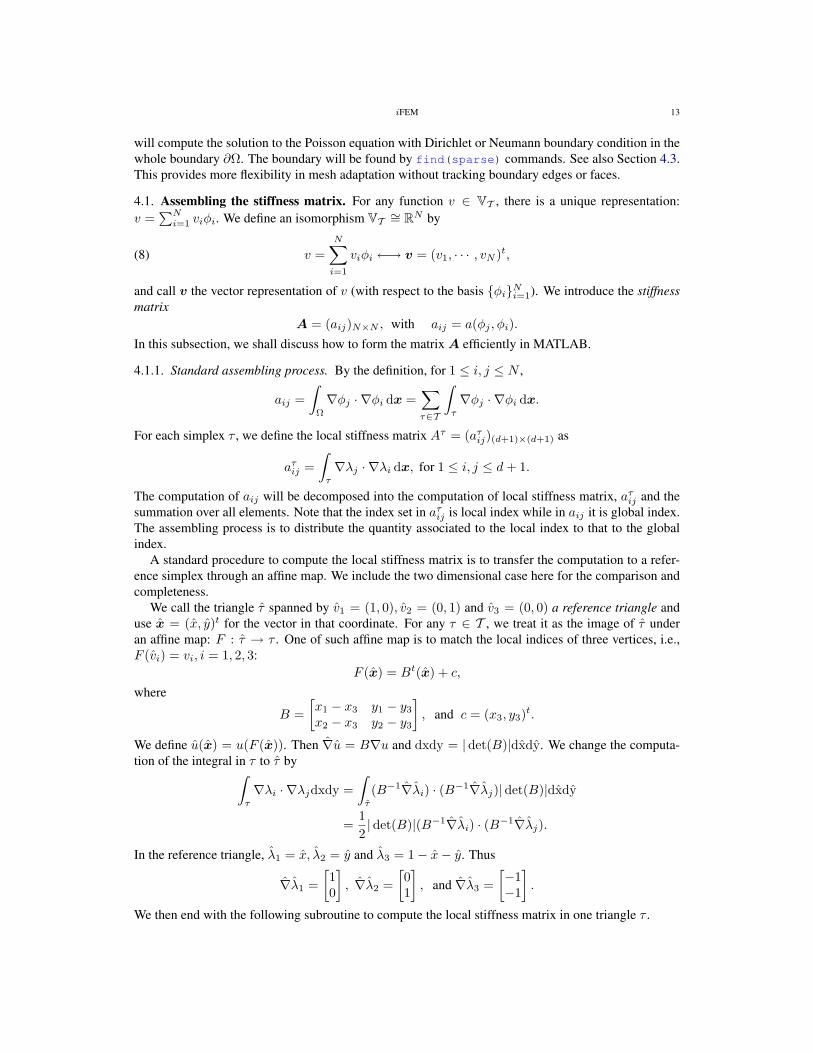
A standard procedure to compute the local stiffness matrix is to transfer the computation to a refer-ence simplex through an affine map. We include the two dimensional case here for the comparison andcompleteness.

We call the triangle τ spanned by v1 = (1, 0), v2 = (0, 1) and v3 = (0, 0) a reference triangle anduse x = (x, y)t for the vector in that coordinate. For any τ ∈ T , we treat it as the image of τ underan affine map: F : τ → τ . One of such affine map is to match the local indices of three vertices, i.e.,F (vi) = vi, i = 1, 2, 3:

F (x) = Bt(x) + c,

where

B =[x1 − x3 y1 − y3

x2 − x3 y2 − y3

], and c = (x3, y3)t.

We define u(x) = u(F (x)). Then ∇u = B∇u and dxdy = |det(B)|dxdy. We change the computa-tion of the integral in τ to τ by∫

τ

∇λi · ∇λjdxdy =∫τ

(B−1∇λi) · (B−1∇λj)|det(B)|dxdy

=12|det(B)|(B−1∇λi) · (B−1∇λj).

In the reference triangle, λ1 = x, λ2 = y and λ3 = 1− x− y. Thus

∇λ1 =[10

], ∇λ2 =

[01

], and ∇λ3 =

[−1−1

].

We then end with the following subroutine to compute the local stiffness matrix in one triangle τ .

14 LONG CHEN

1 function [At,area] = localstiffness(p)

2 At = zeros(3,3);

3 B = [p(1,:)-p(3,:); p(2,:)-p(3,:)];

4 G = [[1,0]’,[0,1]’,[-1,-1]’];

5 area = 0.5*abs(det(B));

6 for i = 1:3

7 for j = 1:3

8 At(i,j) = area*((B\G(:,i))’*(B\G(:,j)));

9 end

10 end

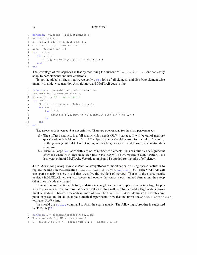
The advantage of this approach is that by modifying the subroutine localstiffness, one can easilyadapt to new elements and new equations.

To get the global stiffness matrix, we apply a for loop of all elements and distribute element-wisequantity to node-wise quantity. A straightforward MATLAB code is like

1 function A = assemblingstandard(node,elem)

2 N=size(node,1); NT=size(elem,1);

3 A=zeros(N,N); %A = sparse(N,N);

4 for t=1:NT

5 At=locatstiffness(node(elem(t,:),:));

6 for i=1:3

7 for j=1:3

8 A(elem(t,i),elem(t,j))=A(elem(t,i),elem(t,j))+At(i,j);

9 end

10 end

11 end

The above code is correct but not efficient. There are two reasons for the slow performance:

(1) The stiffness matrix A is a full matrix which needs O(N2) storage. It will be out of memoryquickly when N is big (e.g., N = 104). Sparse matrix should be used for the sake of memory.Nothing wrong with MATLAB. Coding in other languages also need to use sparse matrix datastructure.

(2) There is a large for loops with size of the number of elements. This can quickly add significantoverhead when NT is large since each line in the loop will be interpreted in each iteration. Thisis a weak point of MATLAB. Vectorization should be applied for the sake of efficiency.

4.1.2. Assembling using sparse matrix. A straightforward modification of using sparse matrix is toreplace the line 3 in the subroutine assemblingstandard by A=sparse(N,N). Then MATLAB willuse sparse matrix to store A and thus we solve the problem of storage. Thanks to the sparse matrixpackage in MATLAB, we can still access and operate the sparse A use standard format and thus keepother lines of code unchanged.

However, as we mentioned before, updating one single element of a sparse matrix in a large loop isvery expensive since the nonzero indices and values vectors will be reformed and a large of data move-ment is involved. Therefore the code in line 8 of assemblingstandard will dominate the whole com-putation procedure. In this example, numerical experiments show that the subroutine assemblingstandardwill take O(N2) time.

We should use sparse command to form the sparse matrix. The following subroutine is suggestedby T. Davis [22].

1 function A = assemblingsparse(node,elem)

2 N = size(node,1); NT = size(elem,1);

3 i = zeros(9*NT,1); j = zeros(9*NT,1); s = zeros(9*NT,1);

iFEM 15

4 index = 0;

5 for t = 1:NT

6 At = localstiffness(node(elem(t,:),:));

7 for ti = 1:3

8 for tj = 1:3

9 index = index + 1;

10 i(index) = elem(t,ti);

11 j(index) = elem(t,tj);

12 s(index) = At(ti,tj);

13 end

14 end

15 end

16 A = sparse(i, j, s, N, N);

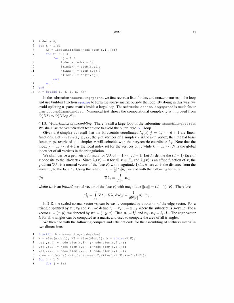
In the subroutine assemblingsparse, we first record a list of index and nonzero entries in the loopand use build-in function sparse to form the sparse matrix outside the loop. By doing in this way, weavoid updating a sparse matrix inside a large loop. The subroutine assemblingsparse is much fasterthan assemblingstandard. Numerical test shows the computational complexity is improved fromO(N2) to O(N logN).

4.1.3. Vectorization of assembling. There is still a large loop in the subroutine aseemblingsparse.We shall use the vectorization technique to avoid the outer large for loop.

Given a d-simplex τ , recall that the barycentric coordinates λj(x), j = 1, · · · , d + 1 are linearfunctions. Let k=elem(t,j), i.e, the j-th vertices of a simplex τ is the k-th vertex, then the hat basisfunction φk restricted to a simplex τ will coincide with the barycentric coordinate λj . Note that theindex j = 1, · · · , d + 1 is the local index set for the vertices of τ , while k = 1, · · · , N is the globalindex set of all vertices in the triangulation.

We shall derive a geometric formula for ∇λi, i = 1, · · · , d + 1. Let Fi denote the (d − 1)-face ofτ opposite to the ith-vertex. Since λi(x) = 0 for all x ∈ Fi, and λi(x) is an affine function of x, thegradient ∇λi is a normal vector of the face Fi with magnitude 1/hi, where hi is the distance from thevertex xi to the face Fi. Using the relation |τ | = 1

d |Fi|hi, we end with the following formula

(9) ∇λi =1

d! |τ |ni,

where ni is an inward normal vector of the face Fi with magnitude ‖ni‖ = (d− 1)!|Fi|. Therefore

aτij =∫τ

∇λi · ∇λj dxdy =1

d!2|τ |ni · nj .

In 2-D, the scaled normal vector ni can be easily computed by a rotation of the edge vector. For atriangle spanned by x1,x2 and x3, we define li = xi+1 − xi−1 where the subscript is 3-cyclic. For avector v = (x, y), we denoted by v⊥ = (−y, x). Then ni = l⊥i and ni · nj = li · lj . The edge vectorli for all triangles can be computed as a matrix and used to compute the area of all triangles.

We then end with the following compact and efficient code for the assembling of stiffness matrix intwo dimensions.

1 function A = assembling(node,elem)

2 N = size(node,1); NT = size(elem,1); A = sparse(N,N);

3 ve(:,:,1) = node(elem(:,3),:)-node(elem(:,2),:);



6 area = 0.5*abs(-ve(:,1,3).*ve(:,2,2)+ve(:,2,3).*ve(:,1,2));

7 for i = 1:3

8 for j = 1:3

16 LONG CHEN

9 Aij = dot(ve(:,:,i),ve(:,:,j),2)./(4*area);;

10 A = A + sparse(elem(:,i),elem(:,j),Aij,N,N);

11 end

12 end

In 3-D, the scaled normal vector ni can be computed by the cross product of two edge vectors. Welist the code below and explain it briefly.

1 function A = assembling3(node,elem)

2 face = [elem(:,[2 4 3]);elem(:,[1 3 4]);elem(:, [1 4 2]);elem(:, [1 2 3])];

3 v12 = node(face(:,2),:)-node(face(:,1),:);

4 v13 = node(face(:,3),:)-node(face(:,1),:);

5 allNormal = cross(v12,v13,2);

6 normal = zeros(NT,3,4);

7 normal(1:NT,:,1) = allNormal(1:NT,:);

8 normal(1:NT,:,2) = allNormal(NT+1:2*NT,:);

9 normal(1:NT,:,3) = allNormal(2*NT+1:3*NT,:);

10 normal(1:NT,:,4) = allNormal(3*NT+1:4*NT,:);

11 v12 = v12(3*NT+1:4*NT,:); v13 = v13(3*NT+1:4*NT,:);

12 v14 = node(elem(:,4),:)-node(elem(:,1),:);

13 volume = dot(cross(v12,v13,2),v14,2)/6;

14 for i = 1:4

15 for j = 1:4

16 Aij = dot(normal(:,:,i),normal(:,:,j),2)./(36*volume);

17 A = A + sparse(elem(:,i),elem(:,j),Aij,N,N);

18 end

19 end

The code in line 2 will collect all faces of the tetrahedron mesh. So the face is of dimension 4NT×3.For each face, we form two edge vectors v12 and v13, and apply the cross product to obtain the scalednormal vector in allNormal matrix. The code in line 6-10 is to reshape the 4NT×3 normal vector to aNT×3×4 matrix. Line 13 use the mix product of three edge vectors to compute the volume and line 14–19 is similar to 2-D case. The introduction of the scaled normal vector ni simplify the implementationand enable us to vectorize the code.

Remark 4.1. The computation of the local stiffness matrix, i.e., the subroutine localstiffness, canbe written in a concise way by avoiding the two inner loops; See [2, 28]. Similarly the small loop fori, j = 1, · · · , d + 1 can be avoid by reshape the vector. But we shall not preform the vectorizationfor these small loops since the gained efficiency is marginal and cannot compensate the reduction ofreadability.

4.2. Right hand side. We define the vector f = (f1, · · · , fN )t by fi =∫

Ωfφi, where φi is the hat

basis at the vertex vi. For quasi-uniform meshes, all simplices are in the same size, while in adaptivefinite element method, some elements with large mesh size could remain unchanged. Therefore, al-though the 1-point quadrature is adequate for linear element on quasi-uniform meshes, to reduce theerror introduced by the numerical quadrature, we compute the load term

∫Ωfφi by 3-points quadrature

rule in 2-D and 4-points rule in 3-D.We list the 2-D code below as an example to emphasis again that the command accumarray is used

to avoid the slow for loop over all elements.

1 mid1 = (node(elem(:,2),:)+node(elem(:,3),:))/2;



4 bt1 = area.*(f(mid2)+f(mid3))/6;


iFEM 17


7 b = accumarray(elem(:),[bt1;bt2;bt3],[N 1]);

4.3. Boundary condition. To build the boundary condition into the matrix equation, we first discussthe data structure to represent Dirichlet boundary ΓD and Neumann boundary ΓN .

We shall use bdEdge(1:NT,1:3) to indicate which edge of each element is on the boundary. Thevalue is the type of boundary condition: 1 for first type, i.e., Dirichlet boundary edges, 2 for sec-ond type, i.e., Neumann boundary edges, and 0 for non-boundary, i.e., interior edges. For example,bdEdge(t,:)=[1 0 2] means, the edge opposite to elem(t,1) is a Dirichlet boundary face, the oneto elem(t,3) is of Neumann type, and the other is an interior edge. The third type of boundary condi-tion, i.e., Robin boundary condition, can be easily added into bdEdge but is not discussed in this paper.We can extract boundary edges from bdEdge using the following code:

1 totalEdge = [elem(:,[2,3]); elem(:,[3,1]); elem(:,[1,2])];

2 isBdEdge = reshape(bdEdge,3*NT,1);

3 Dirichlet = totalEdge((isBdEdge == 1),:);

4 Neumann = totalEdge((isBdEdge == 2),:);

Similarly in 3-D, we use bdFace(1:NT,1:4) to indicate which face of each element is on theboundary and extract different type of boundary faces in this way.

Remark 4.2. The matrix bdFace is sparse but we use dense matrix to store it. It would save storageif we save boundary edges or faces only. The current form is more convenient for the local refinementand coarsening since the update on the boundary can be easily done with the bisection of elements.

We do not save bdFace as a sparse matrix since updating sparse matrix is time consuming. We setup the type of bdEdge to int8 to minimize the waste of spaces.

Remark 4.3. When only Dirichlet or Neumann boundary condition is posed, we do not have to storethe boundary edges or faces. The boundary will be found by

[bdNode,bdEdge] = findboundary(elem)

[bdNode,bdFace] = findboundary3(elem)

for 2-D or 3-D domains, respectively, using find(sparse) commands.

The boundary condition is then treated in the same way as that in [2]. We list the code for 2-D caseand briefly explain it for the completeness.

1 %-------------------- Dirichlet boundary conditions------------------------

2 isBdNode = false(N,1); isBdNode(Dirichlet) = true;

3 bdNode = find(isBdNode);

4 freeNode = find(˜isBdNode);

5 u = zeros(N,1); u(bdNode) = g_D(node(bdNode,:));

6 b = b - A*u;

7 %-------------------- Neumann boundary conditions -------------------------

8 Nve = node(Neumann(:,1),:) - node(Neumann(:,2),:);

9 edgeLength = sqrt(sum(Nve.ˆ2,2));

10 mid = (node(Neumann(:,1),:) + node(Neumann(:,2),:))/2;

11 b = b + accumarray([Neumann(:),ones(2*size(Neumann,1),1)], ...

12 repmat(edgeLength.*g_N(mid)/2,2,1),[N,1]);

Line 1-3 will find all Dirichlet boundary nodes. The Dirichlet boundary condition is posed by assignthe function values at Dirichlet boundary nodes. Note that the vector u is initialized as zero vector.Therefore after line 5, the vector u will represent a function uD ∈ HgD,ΓD

. Writing u = u + uD,finding u is equivalent to finding u ∈ VT ∩H1

0 (Ω) such that a(u, v) = (f, v)− a(uD, v) + (gN , v)ΓN

for all v ∈ VT ∩ H10 (Ω). The modification of the right hand side (f, v) − a(uD, v) is realized by the

18 LONG CHEN

code b=b-A*u in line 6. The boundary integral involving the Neumann boundary part is computed inline 8–12. Note that the code is speed up using accumarray.

Since uD and u use disjoint nodes set, one vector u is used to represent both. The addition of u+uDis realized by assign values to different node sets of the same vector u. We have assigned the value toboundary nodes in line 5. We will compute u, i.e., the value at other nodes (denoted by freeNode), by

(10) u(freeNode)=A(freeNode,freeNode)\b(freeNode).

Here A\b computes A−1b using MATLAB build int direct solver.

5. BISECTION

In this section, we shall discuss bisection methods for the local mesh refinement and efficient imple-mentations of newest vertex bisection in 2-D and longest edge bisection in 3-D. In short, the bisectionmethod will divide one simplex into two children simplicies. Another class of mesh refinement method,known as regular refinement, which divide one simplex into 2d children simplicies, will not be discussedin this paper.

5.1. Bisection methods. In this subsection, we shall present an abstract definition of bisection methodsand review existing bisection methods in 2-D and 3-D.

5.1.1. Abstract definition. Given a simplex τ , we shall choose one of its edges as refinement edge. Alabeled simplex is a pair (τ, e) and a labeled triangulation is a set (T ,L) := (τ, e) : τ ∈ T . Startingfrom an initial triangulation T0, a bisection method consists of:

(1) a rule to assign refinement edges for each element τ ∈ T0;(2) a rule to divide a simplex with a refinement edge into two children simplices;(3) a rule to assign refinement edges to children simplices.

Rule 1 can be described by a mapping T0 → (T0,L) and called initial labeling. This rule is anessential ingredient of bisection methods. Once the initial labeling is given, the subsequent grids inheritlabels according to Rule 3 such that the bisection can proceed. Mathematically, let τ1 and τ2 be twosimplices such that τ1 ∪ τ2 = τ is a simplex. Rule 2 and 3 can be described by a mapping

bτ : (τ, e) → (τ1, e1), (τ2, e2).For a labeled triangulation (T ,L), and a bisection bτ for τ ∈ T , we define a formal addition

T + bτ :=[(T ,L)\(τ, e)

]∪ (τ1, e1), (τ2, e2).

For a sequence of bisections B = (bτ1 , bτ2 , · · · , bτN), we define

(11) T + B := ((T + bτ1) + bτ2) + · · ·+ bτN,

whenever the addition is well defined, i.e., τi should exists in the previous labeled triangulation. Theseadditions are a convenient mathematical description of bisection methods on triangulations.

Given a labeled initial grid T0 and a bisection method, we define

F (T0) = T : there exists a bisection sequence B such that T = T0 + B,and C (T0) = T ∈ F (T0) : T is conforming.

Namely F (T0) contains all triangulations obtained from T0 using this bisection method. But a triangu-lation T ∈ F (T0) could be non-conforming and thus we define C (T0) as a subset of F (T0) containingonly conforming triangulations.

We then define a partial ordering in the set F (T0). We say T2 is a refinement of T1 and denoted byT1 ≤ T2 if there exists a bisection sequence B such that T2 = T1 +B. Given a triangulation T ∈ F (T0),if there exists a triangulation T ∈ C (T0) with minimal number of elements such that T ≤ T , we callT the completion of T .

iFEM 19

CHAPTER 1. CONVERGENCEOF ADAPTIVE FINITE ELEMENTMETHODS 10

Figure 1.1: Edges in bold case are bases

1 2 3

1 1

4 4

2 3 2 3

3 2

2 3

Figure 1.2: Four similarity classes of triangles generated by the newest vertex bisection

1.2 Preliminaries

In this section we shall present some preliminaries needed for the convergence analysis of the

adaptive finite element methods. We first discuss the newest vertex bisection which is the rule

we used to divide the triangles. We then present a quasi-interpolation operator which is crucial

to prove the upper bound of residual type a posteriori error estimator.

Newest vertex bisection

In this subsection we give a brief introduction of the newest vertex bisection and mainly concern

the number of elements added by the completion process. We refer to [31, 42] and [11] for

detailed description of the newest vertex bisection refinement procedure.

Given an initial shape regular triangulation T0 of Ω, it is possible to assign to each τ ∈ T0

exactly one vertex called peak or the newest vertex. The opposite edge of the peak is called base.

The rule of the newest vertex bisection includes: 1) a triangle is divided to two new children

triangles by connecting the peak to the midpoint of the base; 2) the new vertex created at a

midpoint of a base is assigned to be the peak of the children. Sewell [39] showed that all the

decendants of an original triangle fall into four similarity classes (see Figure 1.2) and hence the

angles are bounded away from 0 and π.

To generate a triangulation Tk+1 from previous one Tk, we first mark some of the triangles of

Tk according to some marking strategy and subdivide the marked triangles using newest vertex

bisection to get T ′k+1. The new partition T ′

k+1 might have hanging nodes. We make additional

subdivisions to eliminate the hanging nodes i.e. complete the new partition. The completion is

made by dividing triangles using the designated peaks and base points. Tk+1 will be defined as

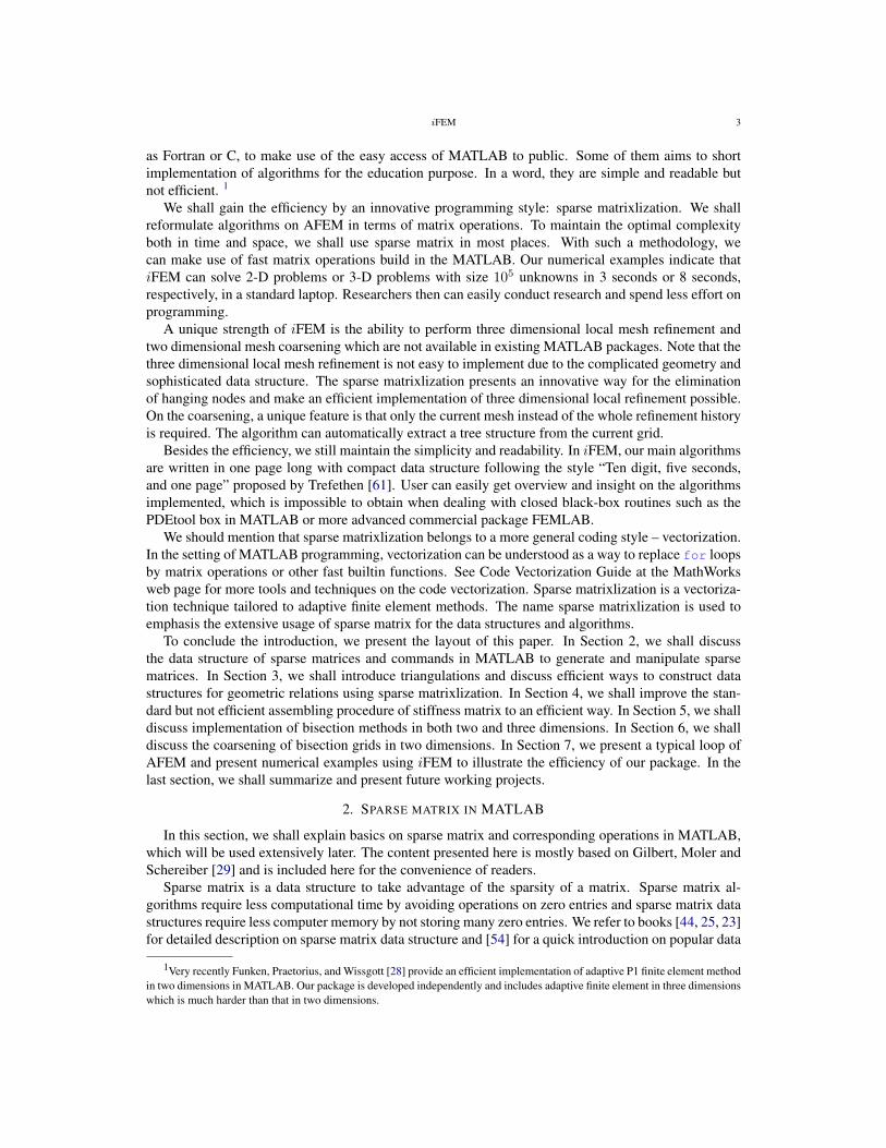
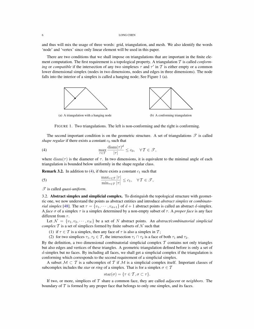
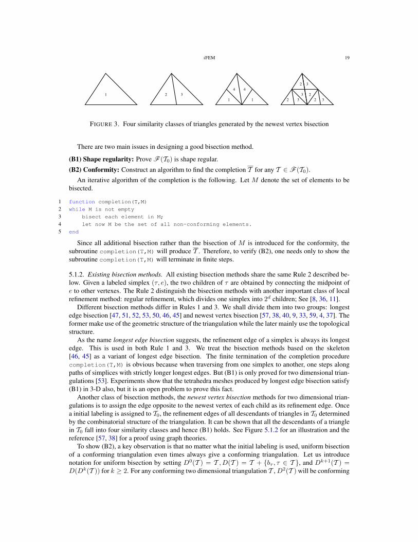
FIGURE 3. Four similarity classes of triangles generated by the newest vertex bisection

There are two main issues in designing a good bisection method.

(B1) Shape regularity: Prove F (T0) is shape regular.

(B2) Conformity: Construct an algorithm to find the completion T for any T ∈ F (T0).

An iterative algorithm of the completion is the following. Let M denote the set of elements to bebisected.

1 function completion(T,M)

2 while M is not empty

3 bisect each element in M;

4 let now M be the set of all non-conforming elements.

5 end

Since all additional bisection rather than the bisection of M is introduced for the conformity, thesubroutine completion(T,M) will produce T . Therefore, to verify (B2), one needs only to show thesubroutine completion(T,M) will terminate in finite steps.

5.1.2. Existing bisection methods. All existing bisection methods share the same Rule 2 described be-low. Given a labeled simplex (τ, e), the two children of τ are obtained by connecting the midpoint ofe to other vertexes. The Rule 2 distinguish the bisection methods with another important class of localrefinement method: regular refinement, which divides one simplex into 2d children; See [8, 36, 11].

Different bisection methods differ in Rules 1 and 3. We shall divide them into two groups: longestedge bisection [47, 51, 52, 53, 50, 46, 45] and newest vertex bisection [57, 38, 40, 9, 33, 59, 4, 37]. Theformer make use of the geometric structure of the triangulation while the later mainly use the topologicalstructure.

As the name longest edge bisection suggests, the refinement edge of a simplex is always its longestedge. This is used in both Rule 1 and 3. We treat the bisection methods based on the skeleton[46, 45] as a variant of longest edge bisection. The finite termination of the completion procedurecompletion(T,M) is obvious because when traversing from one simplex to another, one steps alongpaths of simplices with strictly longer longest edges. But (B1) is only proved for two dimensional trian-gulations [53]. Experiments show that the tetrahedra meshes produced by longest edge bisection satisfy(B1) in 3-D also, but it is an open problem to prove this fact.

Another class of bisection methods, the newest vertex bisection methods for two dimensional trian-gulations is to assign the edge opposite to the newest vertex of each child as its refinement edge. Oncea initial labeling is assigned to T0, the refinement edges of all descendants of triangles in T0 determinedby the combinatorial structure of the triangulation. It can be shown that all the descendants of a trianglein T0 fall into four similarity classes and hence (B1) holds. See Figure 5.1.2 for an illustration and thereference [57, 38] for a proof using graph theories.

To show (B2), a key observation is that no matter what the initial labeling is used, uniform bisectionof a conforming triangulation even times always give a conforming triangulation. Let us introducenotation for uniform bisection by setting D0(T ) = T , D(T ) = T + bτ , τ ∈ T , and Dk+1(T ) =D(Dk(T )) for k ≥ 2. For any conforming two dimensional triangulation T ,D2(T ) will be conforming

20 LONG CHEN

although D(T ) may not. For example, uniform bisect the mesh in Figure 1 (b) using longest edgebisection leads to a non-conforming mesh. By the definition of completion

(12) T ≤ D2(T ), ∀ T ∈ F (T0).

Since all additional bisection rather than the bisection of M is introduced for the conformity, the sub-routine completion(T,M) will produce T .

There are several bisection methods proposed in three and higher dimensions which try to generalizethe newest vertex bisection [9, 33, 59, 4, 37]. Indeed all of these methods are more or less equivalentin Rule 3. We shall not give detailed description of these bisection methods here since the descriptionof Rules 1 and 3 is very technical for three and higher dimensions. In these methods, (B1) is relativelyeasy to prove by showing all descendants of a simplex in T0 fall into similarity classes. Usually (B2)requires special initial labeling, i.e., Rule 1.

For some special triangulations and initial labeling, longest edge bisection and newest vertex bisec-tion are equivalent. For example, for triangulations composed by isosceles right triangles using thelongest edge in Rule 1, then longest bisection and newest vertex bisection coincides. Similar fact holdsfor 3-D triangulations obtained by dividing one cube into six tetrahedron. But in general, these twomethods are quite different. See [38] for a throughly comparison in 2-D.

Remark 5.1. IfDk(T0) is conforming, for any k ≥ 0, there is a recursive algorithm for the completion.But to ensure this condition, special initial labeling is needed. The requirement of such initial labelingis practical in 2-D [38, 40] and more restrictive in three and high dimensions [33, 12, 59, 37, 58].

5.2. Implementation of newest vertex bisection in two dimensions. In this subsection, we shallpresent an efficient completion algorithm which will terminate for arbitrary initial labeling. This com-pletion algorithm is firstly proposed in our recent work [15].

The following subroutine[node,elem,bdEdge] = bisect(node,elem,markedElem,bdEdge)

will refine the current triangulation by bisecting marked elements and minimal neighboring ele-ments to get a conforming and shape regular triangulation. Newest vertex bisection is used. The inputmarkedElem is a vector containing the index of elements to be bisected, and bdEdge stores boundaryedges. The argument bdEdge in the input and output is optional and can be omitted.

5.2.1. Refinement edge. The first question is: how to represent a labeled triangulation? Of coursewe could introduce an additional vector to record the refinement edge of each element. But we havea better way to do that. Recall that our representation of a triangle: elem(t,[1 2 3]) are globalindices of three vertices of the triangle t. The only requirement on the ordering is that the orienta-tion is counter-clockwise. A cyclical permutation of three indices still represents the same triangle.Namely elem(t,[2 3 1]), elem(t,[3 1 2]) represent the same triangle as elem(t,[1 2 3]).We shall use the following rule to record the refinement edge:

(13) The refinement edge of t is elem(t,[2 3]).

That is elem(t,1) will be always the newest vertex of the triangle t. By following this rule, we buildthe labeled triangle into the ordering of the second dimension of the matrix elem.

5.2.2. Completion. We now give a more efficient algorithm, comparing with completion(T,M), forthe completion procedure. A key observation is that since T ≤ D2(T ), the new points added from T toT are middle points of some edges of T . Therefore instead of operating on triangles, we cut necessaryedges first.

Let us denote the refinement edge of τ by cutEdge(τ). For a triangle τ ∈ T , there are at mostthree neighbors of τ . We define the refinement neighbor of τ , denoted by F (τ), as the neighbor sharingthe refinement edge of τ . When cutEdge(τ) is on the boundary, we define F (τ) = τ . Note that

iFEM 21

cutEdge(τ) may not be the refinement edge of F (τ). To ensure the conformity, it suffices to satisfy therule

If cutEdge(τ) is bisected, then cutEdge(F (τ)) should also be bisected.

Given a triangle τ to be bisected, we bisect cutEdge(τ) and check the refinement edge of the re-finement neighbor of τ , i.e., cutEdge(F (τ)). If it is bisected already, we stop. Otherwise, we bisectcutEdge(F (τ)) and check cutEdge(F 2(τ)) and so on. Starting form a marked triangle τ , we then havea flow:

cutEdge(τ)→ cutEdge(F (τ))→ . . .→ cutEdge(Fm(τ)).The flow will end if cutEdge(Fm(τ)) is already bisected. In the best senior, τ and F (τ) share arefinement edge and thus m = 1. In general, the length of the flow could be very long. But since this isa flow among all edges of T , it will stop in finite steps (the worst case is that it traverse all edges).

Using our auxiliary data structure neighbor and elem2edge, this completion can be implementedefficiently; See the following self-explanatory code.

1 isCutEdge = false(NE,1);

2 while sum(markedElem)>0

3 isCutEdge(elem2edge(markedElem,1)) = true;

4 refineNeighbor = neighbor(markedElem,1);

5 markedElem = refineNeighbor(˜isCutEdge(elem2edge(refineNeighbor,1)));

6 end

7 edge2newNode = zeros(NE,1);

8 edge2newNode(isCutEdge) = N+1:N+sum(isCutEdge);

9 node(N+1:N+sum(isCutEdge),:) = (node(edge(isCutEdge,1),:) + node(edge(isCutEdge,2),:))/2;

5.2.3. Bisections of marked triangles. Since we have added all necessary nodes from T to T , we onlyneed to bisect the triangle whose refinement edge is bisected.

1 for k=1:2

2 t = find(edge2newNode(elem2edge(:,1))>0);

3 newNT = length(t);

4 if (newNT == 0), break; end

5 L = t; R = NT+1:NT+newNT;

6 p1 = elem(t,1); p2 = elem(t,2); p3 = elem(t,3);

7 p4 = edge2newNode(elem2edge(t,1));

8 elem(L,:) = [p4, p1, p2];

9 elem(R,:) = [p4, p3, p1];

10 bdEdge(R,[[1 3]) = bdEdge(t,[2 1]);

11 bdEdge(L,[[1 2]) = bdEdge(t,[3 1]);

12 elem2edge(L,1) = elem2edge(t,3);

13 elem2edge(R,1) = elem2edge(t,2);

14 NT = NT + newNT;

15 end

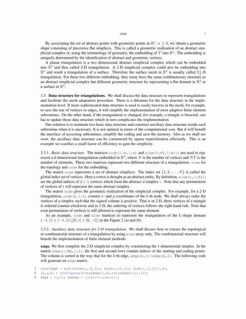
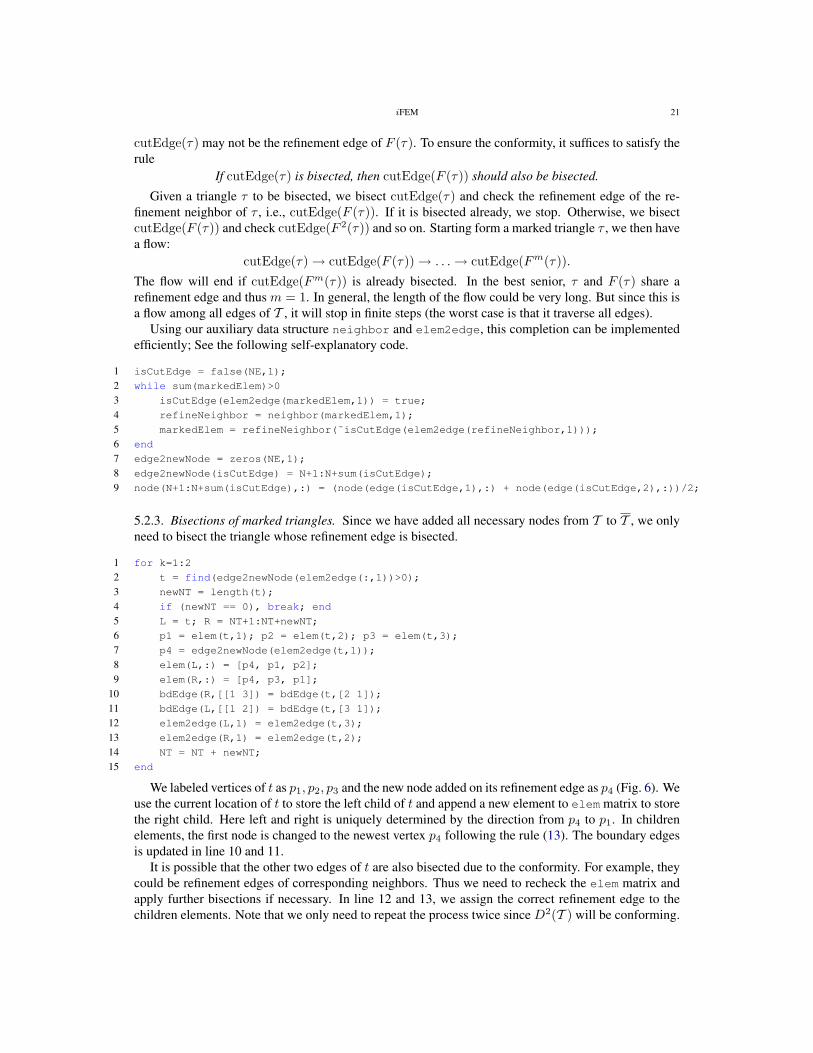
We labeled vertices of t as p1, p2, p3 and the new node added on its refinement edge as p4 (Fig. 6). Weuse the current location of t to store the left child of t and append a new element to elem matrix to storethe right child. Here left and right is uniquely determined by the direction from p4 to p1. In childrenelements, the first node is changed to the newest vertex p4 following the rule (13). The boundary edgesis updated in line 10 and 11.

It is possible that the other two edges of t are also bisected due to the conformity. For example, theycould be refinement edges of corresponding neighbors. Thus we need to recheck the elem matrix andapply further bisections if necessary. In line 12 and 13, we assign the correct refinement edge to thechildren elements. Note that we only need to repeat the process twice since D2(T ) will be conforming.

22 LONG CHEN12 LONG CHEN

1 1 1

2 2 23 3 34 4 4

right left

FIGURE 5. Divide a triangle according to the marked edges

of this new nodes is added into the node matrix. Then we take the neighbor con-

taining its base and repeat the process. The while loop ends until the base of ct

is already marked or it is a boundary edge.

We only append new nodes in the node matrix during the marking. Since we

do not bisect any triangles, we can keep using the auxiliary data structure edge,

dualedge,d2p.

3.4. Refinement. Refinement is short and easy since the conformity is ensured in

the marking step. It is purely local in the sense that we only need to divide each

triangle according to how many edges are marked.

for t=1:NT

base=d2p(elem(t,2),elem(t,3));

if (marker(base)>0)

p=[elem(t,:), marker(base)];

elem=divide(elem,t,p);

left=d2p(p(1),p(2)); right=d2p(p(3),p(1));

if (marker(right)>0)

elem=divide(elem,size(elem,1), [p(4),p(3),p(1),marker(right)]);

end

if (marker(left)>0)

elem=divide(elem,t,[p(4),p(1),p(2),marker(left)]);

end

end

end

%----------------------------------------------------------------------

function elem=divide(elem,t,p)

elem(size(elem,1)+1,:)=[p(4),p(3),p(1)]; elem(t,:)=[p(4),p(1),p(2)];

We first explain the divide function. t is the current triangle to be divided. Its

vertices are p(1), p(2), p(3), and p(4) is the new vertex added in its base (Fig. 5).We modify the current triangle t and add one new element to elem array. Note

that in those elements, the first node is changed to p(4), newest vertex added bythe bisection.

We do a loop for elem matrix. For each triangle, we first check if its base is

marked. If so we divide it and then check the other two edges. If one of them is

marked, we then divide children with suitable order. See Fig. 5 for an illustration.

4. NUMERICAL EXAMPLE

In this section, we shall present a numerical example to show how to cooperate

our bisection algorithm in adaptive finite element methods.

FIGURE 4. Divide a triangle according to the marked edges

5.2.4. Initial labeling. Although the completion procedure we proposed will terminate for arbitrary ini-tial labeling, for the sake of shape regularity, we shall use the longest edge rule in Rule 1. Namely weassign the longest edge as the refinement edge of each triangle in the initial triangulation T0. The sub-routine label is only need for the initial triangulation and thus called outside of the function bisect.It is interesting to note that if we call label inside bisect, then bisect becomes the longest edgebisection.

The following code is self-explanatory.

1 function elem = label(node,elem)

2 totalEdge = [elem(:,[2,3]); elem(:,[3,1]); elem(:,[1,2])];

3 ve = node(totalEdge(:,1),:)-node(totalEdge(:,2),:);

4 edgeLength = reshape(sum(ve.ˆ2,2),size(elem,1),3);

5 [temp,I] = max(edgeLength,[],2);

6 elem((I==2),[1 2 3]) = elem((I==2), [2 3 1]);

7 elem((I==3),[1 2 3]) = elem((I==3), [3 1 2]);

5.3. Implementation of longest edge bisection in three dimensions. We shall implement the longestedge bisection in three dimensions. For this method, the Rule 1 and 3 are pretty simple: we always bisectthe longest edge of a tetrahedron. The completion procedure is the standard one completion(T,M).The function

[node,elem,bdFace] = bisect3(node,elem,markedElem,bdFace)

will refine the current triangulation by bisecting marked elements and minimal neighboring elementsto get a conforming and shape regular triangulation. Longest edge bisection is used in the bisection.The input markedElem is an array containing the index of elements to be bisected, and bdFace storesboundary edges. The argument bdFace in input and output is optional and can be omitted.

5.3.1. Bisection of marked elements. For each element in the marked set M , we can get its refinementedge by finding its longest edge. If the refinement edge is not cut before, we add its middle point as anew node. Otherwise, we need to find out the index of this already added middle point. In 2-D, thisis solved by a pointer vector edge2newNode and the link matrix elem2edge; See the code in Section5.2.2. In 3-D, we use the idea in the construction elem2edge without generating elem2edge matrix.

The following code will find out the refinement edge of each marked element is cut or not.

1 elem = label3(node,elem,markedElem);

2 p1 = elem(markedElem,1); p2 = elem(markedElem,2);

3 ncEdge = find(˜isConforming(1:Ncut));

4 nv2v = sparse([cutEdge(ncEdge,3);cutEdge(ncEdge,3)],...

5 [cutEdge(ncEdge,1);cutEdge(ncEdge,2)],1,N,N);

6 [i,j] = find(nv2v(:,p1).*nv2v(:,p2));

7 isNewCutEdge = true(NM,1);

8 isNewCutEdge(j) = false;

9 ix = find(isNewCutEdge);

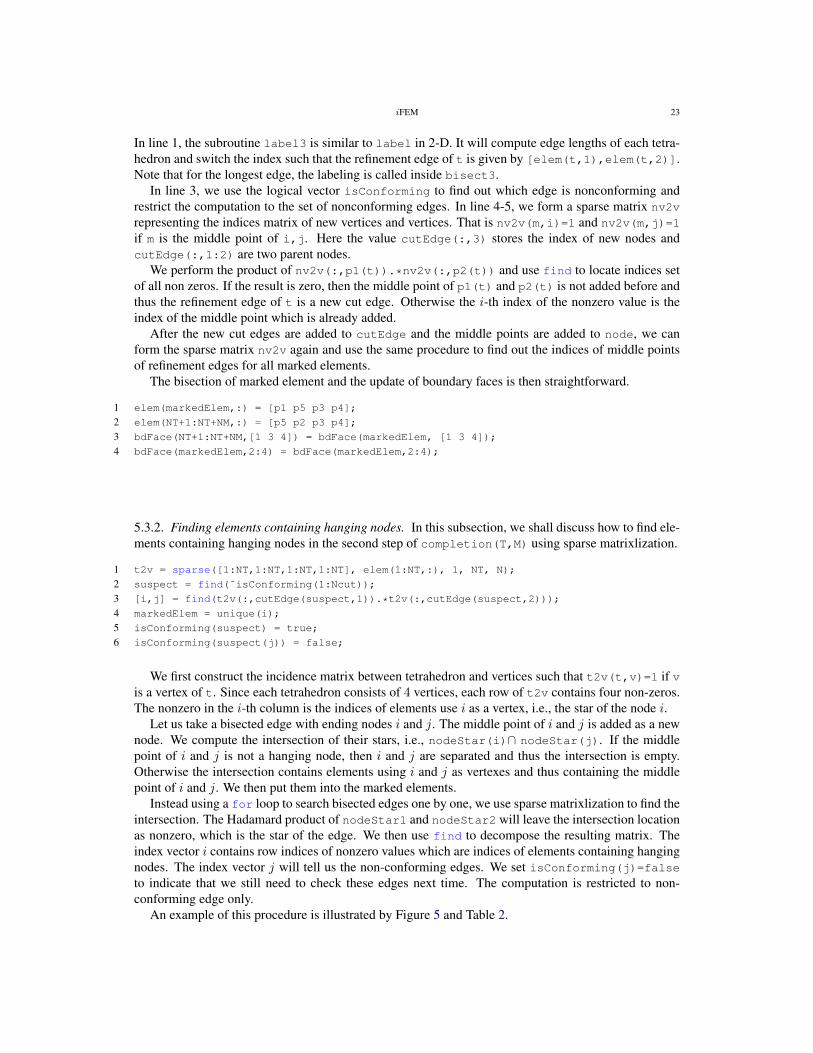
iFEM 23

In line 1, the subroutine label3 is similar to label in 2-D. It will compute edge lengths of each tetra-hedron and switch the index such that the refinement edge of t is given by [elem(t,1),elem(t,2)].Note that for the longest edge, the labeling is called inside bisect3.

In line 3, we use the logical vector isConforming to find out which edge is nonconforming andrestrict the computation to the set of nonconforming edges. In line 4-5, we form a sparse matrix nv2v

representing the indices matrix of new vertices and vertices. That is nv2v(m,i)=1 and nv2v(m,j)=1

if m is the middle point of i,j. Here the value cutEdge(:,3) stores the index of new nodes andcutEdge(:,1:2) are two parent nodes.

We perform the product of nv2v(:,p1(t)).*nv2v(:,p2(t)) and use find to locate indices setof all non zeros. If the result is zero, then the middle point of p1(t) and p2(t) is not added before andthus the refinement edge of t is a new cut edge. Otherwise the i-th index of the nonzero value is theindex of the middle point which is already added.

After the new cut edges are added to cutEdge and the middle points are added to node, we canform the sparse matrix nv2v again and use the same procedure to find out the indices of middle pointsof refinement edges for all marked elements.

The bisection of marked element and the update of boundary faces is then straightforward.

1 elem(markedElem,:) = [p1 p5 p3 p4];

2 elem(NT+1:NT+NM,:) = [p5 p2 p3 p4];

3 bdFace(NT+1:NT+NM,[1 3 4]) = bdFace(markedElem, [1 3 4]);

4 bdFace(markedElem,2:4) = bdFace(markedElem,2:4);

5.3.2. Finding elements containing hanging nodes. In this subsection, we shall discuss how to find ele-ments containing hanging nodes in the second step of completion(T,M) using sparse matrixlization.

1 t2v = sparse([1:NT,1:NT,1:NT,1:NT], elem(1:NT,:), 1, NT, N);

2 suspect = find(˜isConforming(1:Ncut));

3 [i,j] = find(t2v(:,cutEdge(suspect,1)).*t2v(:,cutEdge(suspect,2)));

4 markedElem = unique(i);

5 isConforming(suspect) = true;

6 isConforming(suspect(j)) = false;

We first construct the incidence matrix between tetrahedron and vertices such that t2v(t,v)=1 if vis a vertex of t. Since each tetrahedron consists of 4 vertices, each row of t2v contains four non-zeros.The nonzero in the i-th column is the indices of elements use i as a vertex, i.e., the star of the node i.

Let us take a bisected edge with ending nodes i and j. The middle point of i and j is added as a newnode. We compute the intersection of their stars, i.e., nodeStar(i)∩ nodeStar(j). If the middlepoint of i and j is not a hanging node, then i and j are separated and thus the intersection is empty.Otherwise the intersection contains elements using i and j as vertexes and thus containing the middlepoint of i and j. We then put them into the marked elements.

Instead using a for loop to search bisected edges one by one, we use sparse matrixlization to find theintersection. The Hadamard product of nodeStar1 and nodeStar2 will leave the intersection locationas nonzero, which is the star of the edge. We then use find to decompose the resulting matrix. Theindex vector i contains row indices of nonzero values which are indices of elements containing hangingnodes. The index vector j will tell us the non-conforming edges. We set isConforming(j)=falseto indicate that we still need to check these edges next time. The computation is restricted to non-conforming edge only.

An example of this procedure is illustrated by Figure 5 and Table 2.

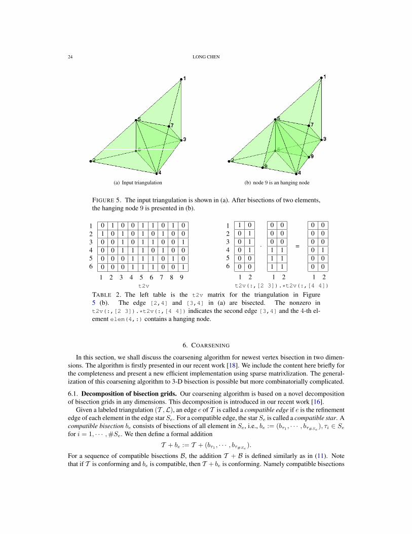
24 LONG CHEN

(a) Input triangulation (b) node 9 is an hanging node

FIGURE 5. The input triangulation is shown in (a). After bisections of two elements,the hanging node 9 is presented in (b).

123456

0 1 0 0 1 1 0 1 01 0 1 0 1 0 1 0 00 0 1 0 1 1 0 0 10 0 1 1 1 0 1 0 00 0 0 1 1 1 0 1 00 0 0 1 1 1 0 0 1

1 2 3 4 5 6 7 8 9t2v

123456

1 00 10 10 10 00 0

·

0 00 00 01 11 11 1

=

0 00 00 00 10 00 0

1 2 1 2 1 2t2v(:,[2 3]).*t2v(:,[4 4])

TABLE 2. The left table is the t2v matrix for the triangulation in Figure5 (b). The edge [2,4] and [3,4] in (a) are bisected. The nonzero int2v(:,[2 3]).*t2v(:,[4 4]) indicates the second edge [3,4] and the 4-th el-ement elem(4,:) contains a hanging node.

6. COARSENING

In this section, we shall discuss the coarsening algorithm for newest vertex bisection in two dimen-sions. The algorithm is firstly presented in our recent work [18]. We include the content here briefly forthe completeness and present a new efficient implementation using sparse matrixlization. The general-ization of this coarsening algorithm to 3-D bisection is possible but more combinatorially complicated.

6.1. Decomposition of bisection grids. Our coarsening algorithm is based on a novel decompositionof bisection grids in any dimensions. This decomposition is introduced in our recent work [16].

Given a labeled triangulation (T ,L), an edge e of T is called a compatible edge if e is the refinementedge of each element in the edge star Se. For a compatible edge, the star Se is called a compatible star. Acompatible bisection be consists of bisections of all element in Se, i.e., be := (bτ1 , · · · , bτ#Se

), τi ∈ Sefor i = 1, · · · ,#Se. We then define a formal addition

T + be := T + (bτ1 , · · · , bτ#Se).

For a sequence of compatible bisections B, the addition T + B is defined similarly as in (11). Notethat if T is conforming and be is compatible, then T + be is conforming. Namely compatible bisections

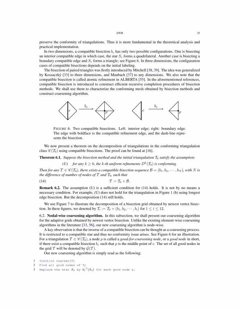
iFEM 25

preserve the conformity of triangulations. Thus it is more fundamental in the theoretical analysis andpractical implementation.

In two dimensions, a compatible bisection be has only two possible configurations. One is bisectingan interior compatible edge in which case, the star Se forms a quadrilateral. Another case is bisecting aboundary compatible edge and Se forms a triangle; see Figure 6. In three dimensions, the configurationcases of compatible bisections depends on the initial labeling.

The bisection of paired triangles was firstly introduced by Mitchell [38, 39]. The idea was generalizedby Kossaczky [33] to three dimensions, and Maubach [37] to any dimensions. We also note that thecompatible bisection is called atomic refinement in ALBERTA [55]. In the aforementioned references,compatible bisection is introduced to construct efficient recursive completion procedures of bisectionmethods. We shall use them to characterize the conforming mesh obtained by bisection methods andconstruct coarsening algorithm.

ebe

p ebe

p

FIGURE 1. Two compatible bisections. Left: interior edge; right:

boundary edge. The vertex near the dot is the newest vertex, the edge

with boldface is the refinement edge, and the dash-line represents the

bisection.

1

FIGURE 6. Two compatible bisections. Left: interior edge; right: boundary edge.The edge with boldface is the compatible refinement edge, and the dash-line repre-sents the bisection.

We now present a theorem on the decomposition of triangulations in the conforming triangulationclass C (T0) using compatible bisections. The proof can be found at [16].

Theorem 6.1. Suppose the bisection method and the initial triangulation T0 satisfy the assumption:

(U) for any k ≥ 0, the k-th uniform refinements Dk(T0) is conforming.

Then for any T ∈ C (T0), there exists a compatible bisection sequence B = (b1, b2, · · · , bN ), with N isthe difference of number of nodes of T and T0, such that

(14) T = T0 + B.Remark 6.2. The assumption (U) is a sufficient condition for (14) holds. It is not by no means anecessary condition. For example, (U) does not hold for the triangulation in Figure 1 (b) using longestedge bisection. But the decomposition (14) still holds.

We use Figure 7 to illustrate the decomposition of a bisection grid obtained by newest vertex bisec-tion. In these figures, we denoted by Ti := T0 + (b1, b2, · · · , bi) for 1 ≤ i ≤ 12.

6.2. Nodal-wise coarsening algorithm. In this subsection, we shall present our coarsening algorithmfor the adaptive grids obtained by newest vertex bisection. Unlike the existing element-wise coarseningalgorithms in the literature [33, 56], our new coarsening algorithm is node-wise.

A key observation is that the inverse of a compatible bisection can be thought as a coarsening process.It is restricted to a compatible star and thus no conformity issue arises. See Figure 6 for an illustration.For a triangulation T ∈ C (T0), a node p is called a good-for-coarsening node, or a good node in short,if there exist a compatible bisection be such that p is the middle point of e. The set of all good nodes inthe grid T will be denoted by G(T ).

Our new coarsening algorithm is simply read as the following:

1 function coarsen(T)

2 Find all good nodes of T;

3 Replace the star Sx by b−1e (Sx) for each good node x.

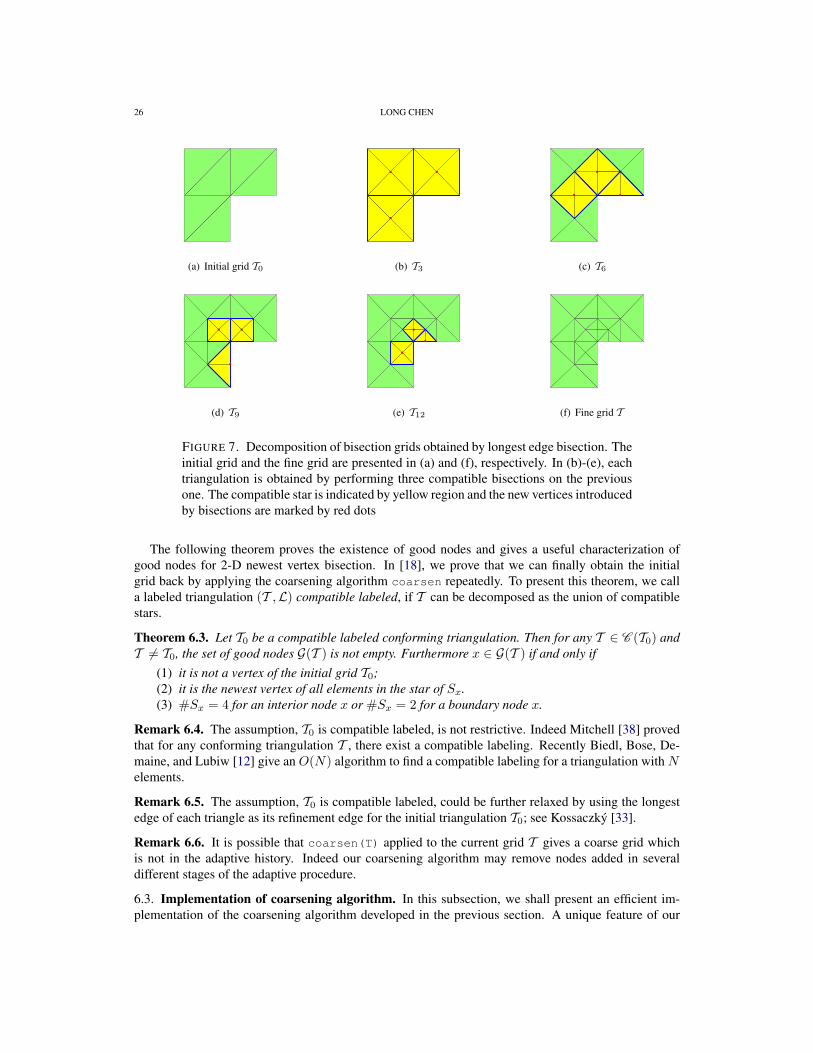
26 LONG CHEN

(a) Initial grid T0 (b) T3 (c) T6

(d) T9 (e) T12 (f) Fine grid T

FIGURE 7. Decomposition of bisection grids obtained by longest edge bisection. Theinitial grid and the fine grid are presented in (a) and (f), respectively. In (b)-(e), eachtriangulation is obtained by performing three compatible bisections on the previousone. The compatible star is indicated by yellow region and the new vertices introducedby bisections are marked by red dots

The following theorem proves the existence of good nodes and gives a useful characterization ofgood nodes for 2-D newest vertex bisection. In [18], we prove that we can finally obtain the initialgrid back by applying the coarsening algorithm coarsen repeatedly. To present this theorem, we calla labeled triangulation (T ,L) compatible labeled, if T can be decomposed as the union of compatiblestars.

Theorem 6.3. Let T0 be a compatible labeled conforming triangulation. Then for any T ∈ C (T0) andT 6= T0, the set of good nodes G(T ) is not empty. Furthermore x ∈ G(T ) if and only if

(1) it is not a vertex of the initial grid T0;(2) it is the newest vertex of all elements in the star of Sx.(3) #Sx = 4 for an interior node x or #Sx = 2 for a boundary node x.

Remark 6.4. The assumption, T0 is compatible labeled, is not restrictive. Indeed Mitchell [38] provedthat for any conforming triangulation T , there exist a compatible labeling. Recently Biedl, Bose, De-maine, and Lubiw [12] give an O(N) algorithm to find a compatible labeling for a triangulation with Nelements.

Remark 6.5. The assumption, T0 is compatible labeled, could be further relaxed by using the longestedge of each triangle as its refinement edge for the initial triangulation T0; see Kossaczky [33].

Remark 6.6. It is possible that coarsen(T) applied to the current grid T gives a coarse grid whichis not in the adaptive history. Indeed our coarsening algorithm may remove nodes added in severaldifferent stages of the adaptive procedure.

6.3. Implementation of coarsening algorithm. In this subsection, we shall present an efficient im-plementation of the coarsening algorithm developed in the previous section. A unique feature of our

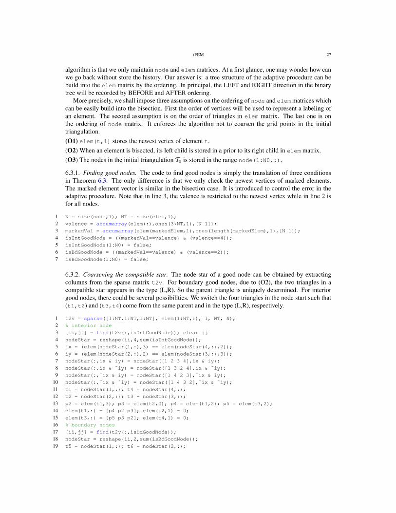
iFEM 27

algorithm is that we only maintain node and elem matrices. At a first glance, one may wonder how canwe go back without store the history. Our answer is: a tree structure of the adaptive procedure can bebuild into the elem matrix by the ordering. In principal, the LEFT and RIGHT direction in the binarytree will be recorded by BEFORE and AFTER ordering.

More precisely, we shall impose three assumptions on the ordering of node and elem matrices whichcan be easily build into the bisection. First the order of vertices will be used to represent a labeling ofan element. The second assumption is on the order of triangles in elem matrix. The last one is onthe ordering of node matrix. It enforces the algorithm not to coarsen the grid points in the initialtriangulation.(O1) elem(t,1) stores the newest vertex of element t.(O2) When an element is bisected, its left child is stored in a prior to its right child in elem matrix.(O3) The nodes in the initial triangulation T0 is stored in the range node(1:N0,:).

6.3.1. Finding good nodes. The code to find good nodes is simply the translation of three conditionsin Theorem 6.3. The only difference is that we only check the newest vertices of marked elements.The marked element vector is similar in the bisection case. It is introduced to control the error in theadaptive procedure. Note that in line 3, the valence is restricted to the newest vertex while in line 2 isfor all nodes.

1 N = size(node,1); NT = size(elem,1);

2 valence = accumarray(elem(:),ones(3*NT,1),[N 1]);

3 markedVal = accumarray(elem(markedElem,1),ones(length(markedElem),1),[N 1]);

4 isIntGoodNode = ((markedVal==valence) & (valence==4));

5 isIntGoodNode(1:N0) = false;

6 isBdGoodNode = ((markedVal==valence) & (valence==2));

7 isBdGoodNode(1:N0) = false;

6.3.2. Coarsening the compatible star. The node star of a good node can be obtained by extractingcolumns from the sparse matrix t2v. For boundary good nodes, due to (O2), the two triangles in acompatible star appears in the type (L,R). So the parent triangle is uniquely determined. For interiorgood nodes, there could be several possibilities. We switch the four triangles in the node start such that(t1,t2) and (t3,t4) come from the same parent and in the type (L,R), respectively.

1 t2v = sparse([1:NT,1:NT,1:NT], elem(1:NT,:), 1, NT, N);

2 % interior node

3 [ii,jj] = find(t2v(:,isIntGoodNode)); clear jj

4 nodeStar = reshape(ii,4,sum(isIntGoodNode));

5 ix = (elem(nodeStar(1,:),3) == elem(nodeStar(4,:),2));

6 iy = (elem(nodeStar(2,:),2) == elem(nodeStar(3,:),3));

7 nodeStar(:,ix & iy) = nodeStar([1 2 3 4],ix & iy);

8 nodeStar(:,ix & ˜iy) = nodeStar([1 3 2 4],ix & ˜iy);

9 nodeStar(:,˜ix & iy) = nodeStar([1 4 2 3],˜ix & iy);

10 nodeStar(:,˜ix & ˜iy) = nodeStar([1 4 3 2],˜ix & ˜iy);

11 t1 = nodeStar(1,:); t4 = nodeStar(4,:);


13 p2 = elem(t1,3); p3 = elem(t2,2); p4 = elem(t1,2); p5 = elem(t3,2);

14 elem(t1,:) = [p4 p2 p3]; elem(t2,1) = 0;

15 elem(t3,:) = [p5 p3 p2]; elem(t4,1) = 0;

16 % boundary nodes

17 [ii,jj] = find(t2v(:,isBdGoodNode));

18 nodeStar = reshape(ii,2,sum(isBdGoodNode));


28 LONG CHEN

20 p2 = elem(t5,3); p3 = elem(t6,2); p4 = elem(t5,2);

21 elem(t5,:) = [p4 p2 p3]; elem(t6,1) = 0;

Remark 6.7. The correct configuration for the node star of an interior good node can be constructed byusing neighbor matrix. But since auxstructure subroutine calls a unique command, the currentimplementation using only one sparse command is more efficient.

6.3.3. Clearance of the empty entries. To efficiently use the memory, we shall empty unused memoryin the node and elem matrices.

1 elem((elem(:,1) == 0),:) = [];

2 node(isIntGoodNode | isBdGoodNode,:) = [];

3 indexMap = zeros(N,1);

4 indexMap(˜(isIntGoodNode | isBdGoodNode))= 1:size(node,1);

5 elem = indexMap(elem);

The clearance of node,elem matrices is relatively easy; See the code line 1 and 2. But we should alsoshift the indices in elem to reflect to the change of node indices. So we build an index map from oldnode index to the new and shortened node index. Then elem is shifted by the index map in line 5.

6.3.4. Update of boundary edges. Since some points are deleted and the node index is shifted, we needto update the boundary edges accordingly. The following code is for this purpose.

1 bdEdge(t1,:) = [bdEdge(t1,2) bdEdge(t2,1) bdEdge(t1,1)];



7. ADAPTIVE FINITE ELEMENT METHODS

Standard adaptive finite element methods (AFEM) based on local mesh refinement can be written asloops of the form

(15) SOLVE → ESTIMATE→ MARK → REFINE/ COARSEN.

More precisely, starting from an initial triangulation T0, to get Tk+1 from Tk for k ≥ 0, we first solve theequation to get the solution uk. The error between the exact solution u and the computed approximationuk is estimated using uk, Tk, and possibly the data f . The error estimator is distributed to element-wiseerror indicator which is used to mark a set of of triangles in Tk. Marked triangles and possible moreneighboring triangles are then refined or coarsened in such a way that the triangulation is still shaperegular and conforming.

7.1. The module SOLVE. We shall not discuss the step SOLVE in this paper. We use the build in direc-tor solver of MATLAB. The performance is acceptable for systems with size less than 1 million. We doimplement the most efficient iterative solver: using multigrid as a preconditioner in the PreconditionedConjugate Gradient method in 2-D. For details, we refer to our recent paper [18].

7.2. The module ESTIMATE. The a posteriori error estimators and indicator are essential part of theESTIMATE step. We use residual type error estimator as an example to illustrate the idea. For anyτ ∈ T and any vT ∈ VT , we define

(16) η(vT , τ) =(‖hτf‖20,τ +

∑e∈∂τ

‖h1/2τ [∇vT · ne]‖20,e

)1/2

,

where hτ = |τ |1/d represents the size of the element and the jump of flux across the side e (edge in 2-Dor face in 3-D) is defined as

[∇vT · νe] = ∇vT · νe|τ1 −∇vT · νe|τ2 ,

iFEM 29

if e = τ1 ∩ τ2 and [∇u · νe] = 0 if e ∈ ∂Ω. Here νe is a fixed unit normal direction of side e.Let u and uT be the exact solution and the linear finite element approximation of the Poisson equation

with pure Dirichilet boundary condition. Then one can prove the error estimator

(17) |u− uT |21 ≤ C∑τ∈T

η2(uτ , τ).

The element wise quantity η(uτ , τ) is called error indicator of τ . Note that it may not be a upper boundof the local error in τ .

The computation of the residual type error indicator is easy using our auxiliary data structure neighbor.Here we take part of codes in estimateresidual3 to explain how to compute the jump of ∇u. Theelement residual is computed using 4-points quadrature rule.

1 [Du,volume,normal] = gradient3(node,elem,u);

2 h = volume.ˆ(1/3);

3 neighbor = auxstructure3(elem);

4 faceJump = dot((Du-Du(neighbor(:,1),:)),normal(:,:,1),2).ˆ2 ...

5 + dot((Du-Du(neighbor(:,2),:)),normal(:,:,2),2).ˆ2 ...

6 + dot((Du-Du(neighbor(:,3),:)),normal(:,:,3),2).ˆ2 ...

7 + dot((Du-Du(neighbor(:,4),:)),normal(:,:,4),2).ˆ2;

8 faceJump = h.ˆ(-1).*faceJump;

Line 1 calls a subroutine gradient3 to compute the gradient of a finite element function u using theformula of ∇λi in (9). The output normal is the scaled normal. Therefore the faceJump is scaledaccordingly in line 8.

Remark 7.1. In iFEM, we also implement recovery type error estimators; See estimateW21 andrecoveryZZ subroutines.

7.3. The module MARK. The a posteriori error estimator is split into local error indicators and theyare then employed to make local modifications by dividing the elements whose error indicator is largeand possibly coarsening the elements whose error indicator is small. The way we mark these elementsinfluences the efficiency of the adaptive algorithm. The traditional maximum marking strategy proposedin the pioneering work of Babuska and Vogelius [5] is to mark triangles τ∗ for refinement such that

(18) η(uT , τ∗) ≥ θmaxτ∈T

η(uT , τ), for some θ ∈ (0, 1).

Similar marking by reversing the inequality in (18) is used for coarsening. Such marking strategy isdesigned to evenly equi-distribute the error. We may leave some exceptional elements and focus on theoverall amounts of the error. This leads to the bulk criterion firstly proposed by Dorfler [24] in order toprove the convergence of the local refinement strategy. With such strategy, one defines the marking setM⊂ T such that

(19)∑τ∈M

η2(uT , τ) ≥ θ∑τ∈T

η2(uT , τ), for some θ ∈ (0, 1).

We implement these two popular marking strategies in mark subroutine where we call (18) as ‘MAX’type and (19) as ‘L2’ type. The default one is the later.

1 function markedElem = mark(elem,eta,theta,method)

2 NT = size(elem,1); isMark = false(NT,1);

3 if (nargin < 4), method = ’L2’; end % default marking is L2 based

4 switch upper(method)

5 case ’MAX’

6 isMark(eta>theta*max(eta))=1;

7 case ’COARSEN’

8 isMark(eta<theta*max(eta))=1;

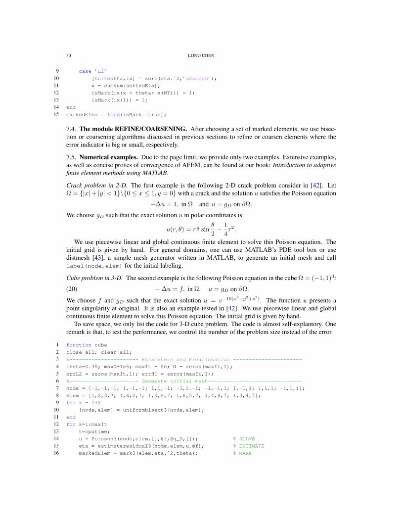
30 LONG CHEN

9 case ’L2’

10 [sortedEta,ix] = sort(eta.ˆ2,’descend’);

11 x = cumsum(sortedEta);

12 isMark(ix(x < theta* x(NT))) = 1;

13 isMark(ix(1)) = 1;

14 end

15 markedElem = find(isMark==true);

7.4. The module REFINE/COARSENING. After choosing a set of marked elements, we use bisec-tion or coarsening algorithms discussed in previous sections to refine or coarsen elements where theerror indicator is big or small, respectively.

7.5. Numerical examples. Due to the page limit, we provide only two examples. Extensive examples,as well as concise proves of convergence of AFEM, can be found at our book: Introduction to adaptivefinite element methods using MATLAB.

Crack problem in 2-D. The first example is the following 2-D crack problem consider in [42]. LetΩ = |x|+ |y| < 1\0 ≤ x ≤ 1, y = 0 with a crack and the solution u satisfies the Poisson equation

−∆u = 1, in Ω and u = gD on ∂Ω.

We choose gD such that the exact solution u in polar coordinates is

u(r, θ) = r12 sin

θ

2− 1

4r2.

We use piecewise linear and global continuous finite element to solve this Poisson equation. Theinitial grid is given by hand. For general domains, one can use MATLAB’s PDE tool box or usedistmesh [43], a simple mesh generator written in MATLAB, to generate an initial mesh and calllabel(node,elem) for the initial labeling.

Cube problem in 3-D. The second example is the following Poisson equation in the cube Ω = (−1, 1)3:

(20) −∆u = f, in Ω, u = gD on ∂Ω.

We choose f and gD such that the exact solution u = e−10(x2+y2+z2). The function u presents apoint singularity at original. It is also an example tested in [42]. We use piecewise linear and globalcontinuous finite element to solve this Poisson equation. The initial grid is given by hand.

To save space, we only list the code for 3-D cube problem. The code is almost self-explantory. Oneremark is that, to test the performance, we control the number of the problem size instead of the error.

1 function cube

2 close all; clear all;

3 %---------------------- Parameters and Preallocation ----------------------

4 theta=0.35; maxN=1e5; maxIt = 50; N = zeros(maxIt,1);

5 errL2 = zeros(maxIt,1); errH1 = zeros(maxIt,1);

6 %---------------------- Generate initial mesh------------------------------

7 node = [-1,-1,-1; 1,-1,-1; 1,1,-1; -1,1,-1; -1,-1,1; 1,-1,1; 1,1,1; -1,1,1];

8 elem = [1,2,3,7; 1,6,2,7; 1,5,6,7; 1,8,5,7; 1,4,8,7; 1,3,4,7];

9 for k = 1:2

10 [node,elem] = uniformbisect3(node,elem);

11 end

12 for k=1:maxIt

13 t=cputime;

14 u = Poisson3(node,elem,[],@f,@g_D,[]); % SOLVE

15 eta = estimateresidual3(node,elem,u,@f); % ESTIMATE

16 markedElem = mark3(elem,eta.ˆ2,theta); % MARK

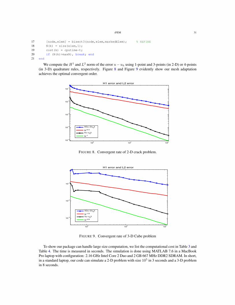
iFEM 31

17 [node,elem] = bisect3(node,elem,markedElem); % REFINE

18 N(k) = size(elem,1);

19 cost(k) = cputime-t;

20 if (N(k)>maxN), break; end

21 end

We compute the H1 and L2 norm of the error u− uh using 1-point and 3-points (in 2-D) or 4-points(in 3-D) quadrature rules, respectively. Figure 8 and Figure 9 evidently show our mesh adaptationachieves the optimal convergent order.

103 104 10510−5

10−4

10−3

10−2

10−1

H1 error and L2 error

||Du−Duh||

N−0.5

||u−uh||

N−1

FIGURE 8. Convergent rate of 2-D crack problem.

103 104 105

10−3

10−2

10−1

H1 error and L2 error

||Du−Duh||

N−1/3

||u−uh||

N−2/3

FIGURE 9. Convergent rate of 3-D Cube problem

To show our package can handle large size computation, we list the computational cost in Table 3 andTable 4. The time is measured in seconds. The simulation is done using MATLAB 7.6 in a MacBookPro laptop with configuration: 2.16 GHz Intel Core 2 Duo and 2 GB 667 MHz DDR2 SDRAM. In short,in a standard laptop, our code can simulate a 2-D problem with size 105 in 3 seconds and a 3-D problemin 8 seconds.

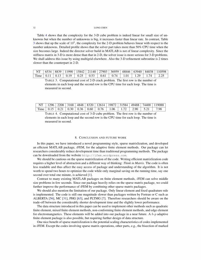
32 LONG CHEN

Table 4 shows that the complexity for the 3-D cube problem is indeed linear for small size of un-knowns but when the number of unknowns is big, it increases faster than linear rate. In contrast, Table3 shows that up the scale of 105, the complexity for the 2-D problem behaves linear with respect to thenumber unknowns. Detailed profile shows that the solver part takes more than 50% CPU time when thesize becomes large. Indeed the director solver build in MATLAB is not of linear complexity. Since thestiffness matrix in 3-D is more dense than that in 2-D, the solver issue is more serious for 3-D problems.We shall address this issue by using multigrid elsewhere. Also the 3-D refinement subroutine is 2 timesslower than the counterpart in 2-D.

NT 6534 8839 11990 15842 21140 27903 36959 48846 63940 84038 110598Time 0.11 0.13 0.19 0.25 0.53 0.61 0.74 1.01 1.29 1.74 2.25

TABLE 3. Computational cost of 2-D crack problem. The first row is the number ofelements in each loop and the second row is the CPU time for each loop. The time ismeasured in second.

NT 1296 2208 3168 4848 8320 12614 19872 31584 49488 74400 119088Time 0.15 0.21 0.30 0.36 0.60 0.76 1.06 1.72 2.90 5.21 7.98

TABLE 4. Computational cost of 3-D cube problem. The first row is the number ofelements in each loop and the second row is the CPU time for each loop. The time ismeasured in second.

8. CONCLUSION AND FUTURE WORK

In this paper, we have introduced a novel programming style, sparse matrixlization, and developedan efficient MATLAB package, iFEM, for the adaptive finite element methods. Our package can letresearchers considerably reduce development time than traditional programming methods. The packagecan be downloaded from the website http://ifem.wordpress.com.

We should be cautious on the sparse matrixlization of the code. Writing efficient matrixlization coderequires a higher level of abstraction and a different way of thinking: Think in Matrix. The code is oftenless readable and thus affect the easy access of package and understanding of the algorithm. It is notworth to spend two hours to optimize the code while only marginal saving on the running time, say onesecond over total one minute, is achieved [1].

Contrast to many existing MATLAB packages on finite element methods, iFEM can solve middlesize problems in few seconds. Since our package heavily relies on the sparse matrix package, we couldfurther improve the performance of iFEM by combining other sparse matrix packages.

We should also mention the limitation of our package. Only linear element and fixed quadrature ruleis implemented. The code is still one magnitude slower than packages written by Fortran or C such asALBERTA [56], MC [31], PHG [63], and PLTMG [7]. Therefore researchers should be aware on thetrade-off between the considerably shorter development time and the slightly lower performance.

The data structure introduced in this paper can be used to implement other methods such as quadraticfinite element, mixed finite element methods, non-conforming finite element methods, and edge elementfor electromangnetics. These elements will be added into our package in a near future. A h-p adaptivefinite element package is also possible, but requiring further design of data structure.

One nice benefit of sparse matrixlization is the potential scaling characteristics of codes implementedin iFEM. Except the codes involving sparse matrix operations, other parts, e.g., the bisection of marked

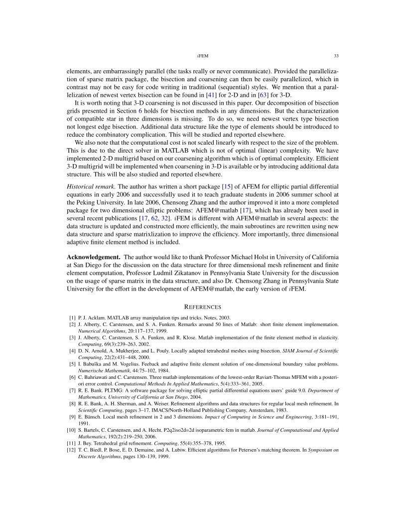
iFEM 33

elements, are embarrassingly parallel (the tasks really or never communicate). Provided the paralleliza-tion of sparse matrix package, the bisection and coarsening can then be easily parallelized, which incontrast may not be easy for code writing in traditional (sequential) styles. We mention that a paral-lelization of newest vertex bisection can be found in [41] for 2-D and in [63] for 3-D.

It is worth noting that 3-D coarsening is not discussed in this paper. Our decomposition of bisectiongrids presented in Section 6 holds for bisection methods in any dimensions. But the characterizationof compatible star in three dimensions is missing. To do so, we need newest vertex type bisectionnot longest edge bisection. Additional data structure like the type of elements should be introduced toreduce the combinatory complication. This will be studied and reported elsewhere.

We also note that the computational cost is not scaled linearly with respect to the size of the problem.This is due to the direct solver in MATLAB which is not of optimal (linear) complexity. We haveimplemented 2-D multigrid based on our coarsening algorithm which is of optimal complexity. Efficient3-D multigrid will be implemented when coarsening in 3-D is available or by introducing additional datastructure. This will be also studied and reported elsewhere.

Historical remark. The author has written a short package [15] of AFEM for elliptic partial differentialequations in early 2006 and successfully used it to teach graduate students in 2006 summer school atthe Peking University. In late 2006, Chensong Zhang and the author improved it into a more completedpackage for two dimensional elliptic problems: AFEM@matlab [17], which has already been used inseveral recent publications [17, 62, 32]. iFEM is different with AFEM@matlab in several aspects: thedata structure is updated and constructed more efficiently, the main subroutines are rewritten using newdata structure and sparse matrixlization to improve the efficiency. More importantly, three dimensionaladaptive finite element method is included.

Acknowledgement. The author would like to thank Professor Michael Holst in University of Californiaat San Diego for the discussion on the data structure for three dimensional mesh refinement and finiteelement computation, Professor Ludmil Zikatanov in Pennsylvania State University for the discussionon the usage of sparse matrix in the data structure, and also Dr. Chensong Zhang in Pennsylvania StateUniversity for the effort in the development of AFEM@matlab, the early version of iFEM.

REFERENCES

[1] P. J. Acklam. MATLAB array manipulation tips and tricks. Notes, 2003.[2] J. Alberty, C. Carstensen, and S. A. Funken. Remarks around 50 lines of Matlab: short finite element implementation.

Numerical Algorithms, 20:117–137, 1999.[3] J. Alberty, C. Carstensen, S. A. Funken, and R. Klose. Matlab implementation of the finite element method in elasticity.

Computing, 69(3):239–263, 2002.[4] D. N. Arnold, A. Mukherjee, and L. Pouly. Locally adapted tetrahedral meshes using bisection. SIAM Journal of Scientific

Computing, 22(2):431–448, 2000.[5] I. Babuska and M. Vogelius. Feeback and adaptive finite element solution of one-dimensional boundary value problems.

Numerische Mathematik, 44:75–102, 1984.[6] C. Bahriawati and C. Carstensen. Three matlab implementations of the lowest-order Raviart-Thomas MFEM with a posteri-

ori error control. Computational Methods In Applied Mathematics, 5(4):333–361, 2005.[7] R. E. Bank. PLTMG: A software package for solving elliptic partial differential equations users’ guide 9.0. Department of

Mathematics, University of California at San Diego, 2004.[8] R. E. Bank, A. H. Sherman, and A. Weiser. Refinement algorithms and data structures for regular local mesh refinement. In

Scientific Computing, pages 3–17. IMACS/North-Holland Publishing Company, Amsterdam, 1983.[9] E. Bansch. Local mesh refinement in 2 and 3 dimensions. Impact of Computing in Science and Engineering, 3:181–191,

1991.[10] S. Bartels, C. Carstensen, and A. Hecht. P2q2iso2d=2d isoparametric fem in matlab. Journal of Computational and Applied

Mathematics, 192(2):219–250, 2006.[11] J. Bey. Tetrahedral grid refinement. Computing, 55(4):355–378, 1995.[12] T. C. Biedl, P. Bose, E. D. Demaine, and A. Lubiw. Efficient algorithms for Petersen’s matching theorem. In Symposium on

Discrete Algorithms, pages 130–139, 1999.

34 LONG CHEN

[13] S. C. Brenner and L. R. Scott. The mathematical theory of finite element methods, volume 15 of Texts in Applied Mathemat-ics. Springer-Verlag, New York, second edition, 2002.

[14] C. Carstensen and R. Klose. Elastoviscoplastic finite element analysis in 100 lines of Matlab. J. Numer. Math., 10(3):157–192, 2002.

[15] L. Chen. Short implementation of bisection in MATLAB. In P. Jorgensen, X. Shen, C.-W. Shu, and N. Yan, editors, RecentAdvances in Computational Sciences – Selected Papers from the International Workship on Computational Sciences and ItsEducation, pages 318 – 332, 2008.

[16] L. Chen, R. H. Nochetto, and J. Xu. Multilevel methods on graded bisection grids I: H1 system. Preprint, 2007.[17] L. Chen and C.-S. Zhang. AFEM@matlab: a Matlab package of adaptive finite element methods. Technique Report, De-

partment of Mathematics, University of Maryland at College Park, 2006.[18] L. Chen and C.-S. Zhang. A coarsening algorithm and multilevel methods on adaptive grids by newest vertex bisection.

Technique Report, Department of Mathematics, University of Maryland at College Park, 2007.[19] J. Chessa. Programing the finite element method with matlab. 2002.[20] P. G. Ciarlet. The Finite Element Method for Elliptic Problems, volume 4 of Studies in Mathematics and its Applications.

North-Holland Publishing Co., Amsterdam-New York-Oxford, 1978.[21] M. Dabrowski, M. Krotkiewski, and D. Schmid. MILAMIN: MATLAB-based finite element method solver for large prob-

lems. Geochemistry Geophysics Geosystems, 9(4), 2008.[22] T. Davis. Creating sparse Finite-Element matrices in MATLAB. http://blogs.mathworks.com/loren/2007/03/01/creating-

sparse-finite-element-matrices-in-matlab/, 2007.[23] T. A. Davis. Direct methods for sparse linear systems, volume 2 of Fundamentals of Algorithms. Society for Industrial and

Applied Mathematics (SIAM), Philadelphia, PA, 2006.[24] W. Dorfler. A convergent adaptive algorithm for Poisson’s equation. SIAM Journal on Numerical Analysis, 33:1106–1124,

1996.[25] I. S. Duff, A. M. Erisman, and J. K. Reid. Direct methods for sparse matrices. Monographs on Numerical Analysis. The

Clarendon Press Oxford University Press, New York, second edition, 1989. Oxford Science Publications.[26] H. C. Elman, A. Ramage, and D. J. Silvester. Algorithm 866: IFISS, a Matlab toolbox for modelling incompressible flow.

ACM Transactions on Mathematical Software, 33(2):14, June 2007. Article 14, 18 pages.[27] H. C. Elman, A. Ramage, and D. J. Silvester. Algorithm 866: Ifiss, a matlab toolbox for modelling incompressible flow.

ACM Trans. Math. Softw., 33(2):14, 2007.[28] S. Funken, D. Praetorius, and P. Wissgott. Efficient implementation of adaptive P1-FEM in MATLAB. Preprint, 2008.[29] J. R. Gilbert, C. Moler, and R. Schreiber. Sparse matrices in MATLAB: design and implementation. SIAM J. Matrix Anal.

Appl., 13(1):333–356, 1992.[30] M. Holst. MCLite: An adaptive multilevel finite element MATLAB package for scalar nonlinear elliptic equations in the

plane. UCSD Technical report and guide to the MCLite software package, 2000.[31] M. Holst. Adaptive numerical treatment of elliptic systems on manifolds. Advances in Computational Mathematics, 15:139–

191, 2001.[32] R. H. W. Hoppe, G. Kanschat, and T. Warburton. Convergence analysis of an adaptive interior penalty discontinuous galerkin

method. Technical report, Texas A & M University, 2007.[33] I. Kossaczky. A recursive approach to local mesh refinement in two and three dimensions. Journal of Computational and

Applied Mathematics, 55:275–288, 1994.[34] Y. W. Kwon and H. Bang. The finite element method using MATLAB. CRC Mechanical Engineering Series. Chapman &

Hall/CRC, Boca Raton, FL, second edition, 2000. With 1 CD-ROM (Windows 95, 98 or NT4.0).[35] J. Li and Y.-T. Chen. Computational Partial Differential Equations Using MATLAB. Applied Mathematics & Nonlinear

Science. Chapman & Hall/CRC, 2008.[36] A. Liu and B. Joe. Quality local refinement of tetrahedral meshes based on bisection. SIAM Journal on Scientific Computing,

16(6):1269–1291, 1995.[37] J. Maubach. Local bisection refinement for n-simplicial grids generated by reflection. SIAM Journal of Scientific Computing,

16(1):210–227, 1995.[38] W. F. Mitchell. Unified Multilevel Adaptive Finite Element Methods for Elliptic Problems. PhD thesis, University of Illinois

at Urbana-Champaign, 1988.[39] W. F. Mitchell. A comparison of adaptive refinement techniques for elliptic problems. ACM Transactions on Mathematical

Software (TOMS) archive, 15(4):326 – 347, 1989.[40] W. F. Mitchell. Optimal multilevel iterative methods for adaptive grids. SIAM Journal on Scientific and Statistical Comput-

ing, 13:146–167, 1992.[41] W. F. Mitchell. A refinement-tree based partitioning method for dynamic load balancing with adaptively refined grids.

Journal of Parallel and Distributed Computing, 67(4):417–429, 2007.[42] P. Morin, R. H. Nochetto, and K. G. Siebert. Convergence of adaptive finite element methods. SIAM Review, 44(4):631–658,

2002.[43] P.-O. Persson and G. Strang. A simple mesh generator in matlab. SIAM Review, 46(2):329–345, 2004.

iFEM 35

[44] S. Pissanetsky. Sparse matrix technology. Academic Press, 1984.[45] A. Plaza and G. F. Carey. Local refinement of simplicial grids based on the skeleton. Applied Numerical Mathematics,

32(2):195–218, 2000.[46] A. Plaza, M. A. Padron, and G. F. Carey. A 3d refinement/derefinement algorithm for solving evolution problems. Applied

Numerical Mathematics, 32(4):401–418, 2000.[47] A. Plaza and M.-C. Rivara. Mesh refinement based on the 8-tetrahedra longest-edge partition. 12th meshing roundtable,

2003.[48] K. Polthier. Computational aspects of discrete minimal surfaces. In Global theory of minimal surfaces, volume 2 of Clay

Math. Proc., pages 65–111. Amer. Math. Soc., Providence, RI, 2005.[49] C. Pozrikidis. Introduction To Finite And Spectral Element Methods Using Matlab. Chapman & Hall/CRC, 2005.[50] M. C. Rivara. Mesh refinement processes based on the generalized bisection of simplices. SIAM Journal on Numerical

Analysis, 21:604–613, 1984.[51] M.-C. Rivara and P. Inostroza. Using longest-side bisection techniques for the automatic refinement fo Delaunay triangula-

tions. International Journal for Numerical Methods in Engineering, 40:581–597, 1997.[52] M. C. Rivara and G. Iribarren. The 4-triangles longest-side partition of triangles and linear refinement algorithms. Mathe-

mathics of Computation, 65(216):1485–1501, 1996.[53] M. C. Rivara and M. Venere. Cost analysis of the longest-side (triangle bisection) refinement algorithms for triangulations.

Engineering with Computers, 12:224–234, 1996.[54] Y. Saad. Iterative methods for sparse linear systems. Society for Industrial and Applied Mathematics, Philadelphia, PA,

second edition, 2003.[55] A. Schmidt and K. G. Siebert. Design of adaptive finite element software, volume 42 of Lecture Notes in Computa-

tional Science and Engineering. Springer-Verlag, Berlin, 2005. The finite element toolbox ALBERTA, With 1 CD-ROM(Unix/Linux).

[56] A. Schmidt and K. G. Siebert. The finite element toolbox ALBERTA. Springer-Verlag, Berlin, 2005.[57] E. G. Sewell. Automatic generation of triangulations for piecewise polynomial approximation. In Ph. D. dissertation. Purdue

Univ., West Lafayette, Ind., 1972.[58] R. Stevenson. The completion of locally refined simplicial partitions created by bisection. Mathemathics of Computation,

77:227–241, 2008.[59] C. T. Traxler. An algorithm for adaptive mesh refinement in n dimensions. Computing, 59(2):115–137, 1997.[60] L. N. Trefethen. Spectral methods in MATLAB, volume 10 of Software, Environments, and Tools. Society for Industrial and

Applied Mathematics (SIAM), Philadelphia, PA, 2000.[61] L. N. Trefethen. Ten digit algorithms. Mitchell Lecture, June 2005.[62] J. Xu, Y. Zhu, and Q. Zou. Convergence analysis of adaptive finite volume element methods for general elliptic equations.

(submitted), 2006.[63] L. Zhang. A parallel algorithm for adaptive local refinement of tetrahedral meshes using bisection. NUMERICAL MATHE-

MATICS: Theory, Methods and Applications, 2008.

DEPARTMENT OF MATHEMATICS, UNIVERSITY OF CALIFORNIA AT IRVINE, IRVINE, CA 92697E-mail address: [email protected]

iFEM: AN INNOVATIVE FINITE ELEMENT METHOD PACKAGE …

Documents

Transcript of iFEM: AN INNOVATIVE FINITE ELEMENT METHOD PACKAGE …