IEOR E4602: Quantitative Risk Management Fall 2016 2016...

IEOR E4602: Quantitative Risk Management Fall 2016c© 2016 by Martin Haugh

Asset Allocation and Risk Management

These lecture notes provide an introduction to asset allocation and risk management. We begin with a briefreview of: (i) the mean-variance analysis of Markowitz (1952) and (ii) the Capital Asset Pricing Model (CAPM).We also review the problems associated with implementing mean-variance analysis in practice and discuss someapproaches for tackling these problems. We then discuss the Black-Litterman approach for incorporatingsubjective views on the markets and also describe some simple extensions of this approach. Mean -Value-at-Risk (Mean-VaR) portfolio optimization is also studied and we highlight how this is generally a badidea as the optimal solution can often inherit the less desirable properties of VaR. Finally we discuss some recentand very useful results for solving mean-CVaR optimization problems. These results lead to problemformulations and techniques that can be useful in many settings including non-Gaussian settings.

We will only briefly discuss issues related to parameter estimation in these notes. This is a very important topicas optimal asset allocations are typically very sensitive to the estimated expected returns. Estimated covariancematrices also play an important role and so many estimation techniques including shrinkage, Bayesian and robustestimation techniques are employed in practice. It is also worth mentioning that in practice estimation errors areoften significant and this often results in the “optimal portfolios” performing no better than portfolios chosen bysimple heuristics. Nonetheless, some of the techniques we describe in these notes can be particularly useful whenwe have strong views on the market that we wish to incorporate into our portfolio selection. They are also usefulin settings where it is desirable to control extreme downside risks such as the CVaR of a portfolio.

1 Review of Mean-Variance Analysis and the CAPM

Consider a one-period market with n securities which have identical expected returns and variances, i.e.E[Ri] = µ and Var(Ri) = σ2 for i = 1, . . . , n. We also suppose Cov(Ri, Rj) = 0 for all i 6= j. Let wi denotethe fraction of wealth invested in the ith security at time t = 0. Note that we must have

∑ni=1 wi = 1 for any

portfolio. Consider now two portfolios:

Portfolio A: 100% invested in security # 1 so that w1 = 1 and wi = 0 for i = 2, . . . , n.

Portfolio B: An equi-weighted portfolio so that wi = 1/n for i = 1, . . . , n.

Let RA and RB denote the random returns of portfolios A and B, respectively. We immediately have

E[RA] = E[RB ] = µ

Var(RA) = σ2

Var(RB) = σ2/n.

The two portfolios therefore have the same expected return but very different return variances. A risk-averseinvestor should clearly prefer portfolio B because this portfolio benefits from diversification without sacrificingany expected return. This was the cental insight of Markowitz who (in his framework) recognized that investorsseek to minimize variance for a given level of expected return or, equivalently, they seek to maximize expectedreturn for a given constraint on variance.

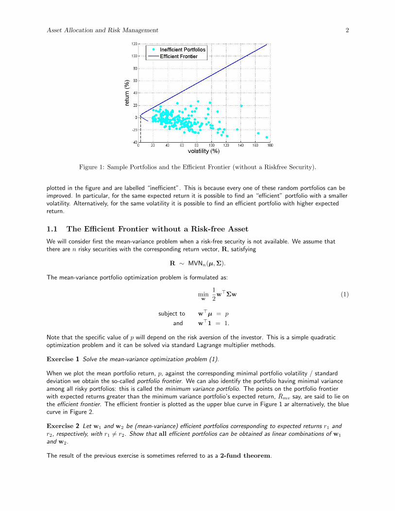
Before formulating and solving the mean variance problem consider Figure 1 below. There were n = 8 securitieswith given mean returns, variances and covariances. We generated m = 200 random portfolios from these nsecurities and computed the expected return and volatility, i.e. standard deviation, for each of them. They are

Asset Allocation and Risk Management 2

Figure 1: Sample Portfolios and the Efficient Frontier (without a Riskfree Security).

plotted in the figure and are labelled “inefficient”. This is because every one of these random portfolios can beimproved. In particular, for the same expected return it is possible to find an “efficient” portfolio with a smallervolatility. Alternatively, for the same volatility it is possible to find an efficient portfolio with higher expectedreturn.

1.1 The Efficient Frontier without a Risk-free Asset

We will consider first the mean-variance problem when a risk-free security is not available. We assume thatthere are n risky securities with the corresponding return vector, R, satisfying

R ∼ MVNn(µ,Σ).

The mean-variance portfolio optimization problem is formulated as:

minw

1

2w>Σw (1)

subject to w>µ = p

and w>1 = 1.

Note that the specific value of p will depend on the risk aversion of the investor. This is a simple quadraticoptimization problem and it can be solved via standard Lagrange multiplier methods.

Exercise 1 Solve the mean-variance optimization problem (1).

When we plot the mean portfolio return, p, against the corresponding minimal portfolio volatility / standarddeviation we obtain the so-called portfolio frontier. We can also identify the portfolio having minimal varianceamong all risky portfolios: this is called the minimum variance portfolio. The points on the portfolio frontierwith expected returns greater than the minimum variance portfolio’s expected return, Rmv say, are said to lie onthe efficient frontier. The efficient frontier is plotted as the upper blue curve in Figure 1 ar alternatively, the bluecurve in Figure 2.

Exercise 2 Let w1 and w2 be (mean-variance) efficient portfolios corresponding to expected returns r1 andr2, respectively, with r1 6= r2. Show that all efficient portfolios can be obtained as linear combinations of w1

and w2.

The result of the previous exercise is sometimes referred to as a 2-fund theorem.


1.2 The Efficient Frontier with a Risk-free Asset

We now assume that there is a risk-free security available with risk-free rate equal to rf . Letw := (w1, . . . , wn)′ be the vector of portfolio weights on the n risky assets so that 1−

∑ni=1 wi is the weight on

the risk-free security. An investor’s portfolio optimization problem may then be formulated as

minw

1

2w>Σw (2)

subject to

(1−

n∑i=1

wi

)rf + w>µ = p.

The optimal solution to (2) is given byw = ξ Σ−1(µ− rf1) (3)

where ξ := σ2min/(p− rf ) and σ2

min is the minimized variance, i.e., twice the value of the optimal objectivefunction in (2). It satisfies

σ2min =

(p− rf )2

(µ− rf1)> Σ−1 (µ− rf1)(4)

where 1 is an n× 1 vector of ones. While ξ (or p) depends on the investor’s level of risk aversion it is ofteninferred from the market portfolio. For example, if we take p− rf to denote the average excess market returnand σ2

min to denote the variance of the market return, then we can take σ2min/(p− rf ) as the average or market

value of ξ.

Suppose now that rf < Rmv. When we allow our portfolio to include the risk-free security the efficient frontierbecomes a straight line that is tangential to the risky efficient frontier and with a y-intercept equal to therisk-free rate. This is plotted as the red line in Figure 2. That the efficient frontier is a straight line when weinclude the risk-free asset is also clear from (4) where we see that σmin is linear in p. Note that this result is a1-fund theorem since every investor will optimally choose to invest in a combination of the risk-free securityand a single risky portfolio, i.e. the tangency portfolio. The tangency portfolio, w∗, is given by the optimalw of (3) except that it must be scaled so that its component sum to 1. (This scaled portfolio will not dependon p.)

Exercise 3 Without using (4) show that the efficient frontier is indeed a straight line as described above.Hint: consider forming a portfolio of the risk-free security with any risky security or risky portfolio. Show thatthe mean and standard deviation of the portfolio varies linearly with α where α is the weight on therisk-free-security. The conclusion should now be clear.

Exercise 4 Describe the efficient frontier if no borrowing is allowed.

The Sharpe ratio of a portfolio (or security) is the ratio of the expected excess return of the portfolio to theportfolio’s volatility. The Sharpe optimal portfolio is the portfolio with maximum Sharpe ratio. It isstraightforward to see in our mean-variance framework (with a risk-free security) that the tangency portfolio,w∗, is the Sharpe optimal portfolio.

1.3 Including Portfolio Constraints

We can easily include linear portfolio constraints in the problem formulation and still easily solve the resultingquadratic program. No-borrowing or no short-sales constraints are examples of linear constraints as are leverageand sector constraints. While analytic solutions are generally no longer available, the resulting problems are stilleasy to solve numerically. In particular, we can still determine the efficient frontier.


Figure 2: The Efficient Frontier with a Riskfree Security.

1.4 Weaknesses of Traditional Mean-Variance Analysis

The traditional mean-variance analysis of Markowitz has many weaknesses when applied naively in practice.They include:

1. The tendency to produce extreme portfolios combining extreme shorts with extreme longs. As a result,portfolio managers generally do not trust these extreme weights. This problem is typically caused byestimation errors in the mean return vector and covariance matrix.

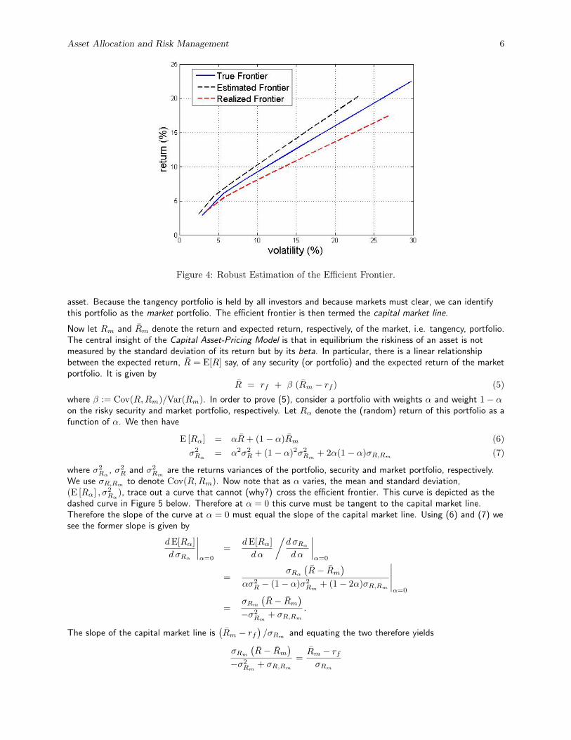
Figure 3: The Efficient Frontier, Estimated Frontiers and Realized Frontiers.

Consider Figure 3, for example, where we have plotted the same efficient frontier (of risky securities) as inFigure 2. In practice, investors can never compute this frontier since they do not know the true meanvector and covariance matrix of returns. The best we can hope to do is to approximate it. But how mightwe do this? One approach would be to simply estimate the mean vector and covariance matrix usinghistorical data. Each of the black dashed curves in Figure 3 is an estimated frontier that we computed by:(i) simulating m = 24 sample returns from the true (in this case, multivariate normal) distribution (ii)estimating the mean vector and covariance matrix from this simulated data and (iii) using these estimatesto generate the (estimated) frontier. Note that the blue curve in Figure 3 is the true frontier computedusing the true mean vector and covariance matrix.

The first observation is that the estimated frontiers are quite random and can differ greatly from the true


frontier. They may lie below or above the true frontier or they may cross it and an investor who uses suchan estimated frontier to make investment decisions may end up choosing a poor portfolio. How poor? Thedashed red curves in Figure 3 are the realized frontiers that depict the true portfolio mean - volatilitytradeoff that results from making decisions based on the estimated frontiers. In contrast to the estimatedfrontiers, the realized frontiers must always (why?) lie below the true frontier. In Figure 3 some of therealized frontiers lie very close to the true frontier and so in these cases an investor would do very well.But in other cases the realized frontier is far from the (generally unobtainable) true efficient frontier.

These examples serve to highlight the importance of estimation errors in any asset allocation procedure.Note also that if we had assumed a heavy-tailed distribution for the true distribution of portfolio returnsthen we might expect to see an even greater variety of sample mean-standard deviation frontiers. Inaddition, it is worth emphasizing that in practice we may not have as many as 24 relevant observationsavailable. For example, if our data observations are weekly returns, then using 24 of them to estimate thejoint distribution of returns is hardly a good idea since we are generally more concerned with estimatingconditional return distributions and so more weight should be given to more recent returns. A moresophisticated estimation approach should therefore be used in practice. More generally, it must be statedthat estimating expected returns using historical data is very problematic and is not advisable!

2. The portfolio weights tend to be extremely sensitive to very small changes in the expected returns. Forexample, even a small increase in the expected return of just one asset can dramatically alter the optimalcomposition of the entire portfolio. Indeed let w and w denote the true optimal and estimated optimalportfolios, respectively, corresponding to the true mean return vector, µ, and the sample mean returnvector, µ, respectively. Then Best and Grauer (19911) showed that

||w − w|| ≤ ξ ||µ− µ|| 1

γmin

(1 +

γmaxγmin

)where γmax and γmin are the largest and smallest eigen values, respectively, of the covariance matrix, Σ.Therefore the sensitivity of the portfolio weights to errors in the mean return vector grows as the ratioγmax/γmin grows. But this ratio, when applied to the estimated covariance matrix, Σ, typically becomeslarge as the number of asset increases and the number of sample observations is held fixed. As a result,we can expect large errors for large portfolios with relatively few observations.

3. While it is commonly believed that errors in the estimated means are of much greater significance, errorsin estimated covariance matrices can also have considerable impact. While it is generally easier toestimate covariances than means, the presence of heavy tails in the return distributions can result insignificant errors in covariance estimates as well. These problems can be mitigated to varying extentsthrough the use of more robust estimation techniques.

As a result of these weaknesses, portfolio managers traditionally have had little confidence in mean-varianceanalysis and therefore applied it very rarely in practice. Efforts to overcome these problems include the use ofbetter estimation techniques such as the use of shrinkage estimators, robust estimators and Bayesian techniquessuch as the Black-Litterman framework introduced in the early 1990’s. (In addition to mitigating the problem ofextreme portfolios, the Black-Litterman framework allows users to specify their own subjective views on themarket in a consistent and tractable manner.) Many of these techniques are now used routinely in general assetallocation settings. It is worth mentioning that the problem of extreme portfolios can also be mitigated in partby placing no short-sales and / or no-borrowing constraints on the portfolio.In Figure 4 above we have shown an estimated frontier that was computed using a more robust estimationprocedure. We see that it lies much closer to the true frontier which is also the case with it’s correspondingrealized frontier.

1.5 The Capital Asset Pricing Model (CAPM)

If every investor is a mean-variance optimizer then we can see from Figure 2 and our earlier discussion that eachof them will hold the same tangency portfolio of risky securities in conjunction with a position in the risk-free

1Sensitivity Analysis for Mean-Variance Portfolio Problems, Management Science, 37 (August), 980-989.


Figure 4: Robust Estimation of the Efficient Frontier.

asset. Because the tangency portfolio is held by all investors and because markets must clear, we can identifythis portfolio as the market portfolio. The efficient frontier is then termed the capital market line.

Now let Rm and Rm denote the return and expected return, respectively, of the market, i.e. tangency, portfolio.The central insight of the Capital Asset-Pricing Model is that in equilibrium the riskiness of an asset is notmeasured by the standard deviation of its return but by its beta. In particular, there is a linear relationshipbetween the expected return, R = E[R] say, of any security (or portfolio) and the expected return of the marketportfolio. It is given by

R = rf + β (Rm − rf ) (5)

where β := Cov(R,Rm)/Var(Rm). In order to prove (5), consider a portfolio with weights α and weight 1− αon the risky security and market portfolio, respectively. Let Rα denote the (random) return of this portfolio as afunction of α. We then have

E [Rα] = αR+ (1− α)Rm (6)

σ2Rα = α2σ2

R + (1− α)2σ2Rm + 2α(1− α)σR,Rm (7)

where σ2Rα

, σ2R and σ2

Rmare the returns variances of the portfolio, security and market portfolio, respectively.

We use σR,Rm to denote Cov(R,Rm). Now note that as α varies, the mean and standard deviation,(E [Rα] , σ2

Rα), trace out a curve that cannot (why?) cross the efficient frontier. This curve is depicted as the

dashed curve in Figure 5 below. Therefore at α = 0 this curve must be tangent to the capital market line.Therefore the slope of the curve at α = 0 must equal the slope of the capital market line. Using (6) and (7) wesee the former slope is given by

dE[Rα]

d σRα

∣∣∣∣α=0

=dE[Rα]

dα

/d σRαdα

∣∣∣∣α=0

=σRα

(R− Rm

)ασ2

R − (1− α)σ2Rm

+ (1− 2α)σR,Rm

∣∣∣∣∣α=0

=σRm

(R− Rm

)−σ2

Rm+ σR,Rm

.

The slope of the capital market line is(Rm − rf

)/σRm and equating the two therefore yields

σRm(R− Rm

)−σ2

Rm+ σR,Rm

=Rm − rfσRm


Figure 5: Proving the CAPM relationship.

which upon simplification gives (5).

The CAPM result is one of the most famous results in all of finance and, even though it arises from a simpleone-period model, it provides considerable insight to the problem of asset-pricing. For example, it is well-knownthat riskier securities should have higher expected returns in order to compensate investors for holding them.But how do we measure risk? Counter to the prevailing wisdom at the time the CAPM was developed, theriskiness of a security is not measured by its return volatility. Instead it is measured by its beta which isproportional to its covariance with the market portfolio. This is a very important insight. Nor, it should benoted, does this contradict the mean-variance formulation of Markowitz where investors do care about returnvariance. Indeed, we derived the CAPM from mean-variance analysis!

Exercise 5 Why does the CAPM result not contradict the mean-variance problem formulation where investorsdo measure a portfolio’s risk by its variance?

The CAPM is an example of a so-called 1-factor model with the market return playing the role of the singlefactor. Other factor models can have more than one factor. For example, the Fama-French model has threefactors, one of which is the market return. Many empirical research papers have been written to test the CAPM.Such papers usually perform regressions of the form

Ri − rf = αi + βi (Rm − rf ) + εi

where αi (not to be confused with the α we used in the proof of (5)) is the intercept and εi is the idiosyncraticor residual risk which is assumed to be independent of Rm and the idiosyncratic risk of other securities. If theCAPM holds then we should be able to reject the hypothesis that αi 6= 0. The evidence in favor of the CAPM ismixed. But the language inspired by the CAPM is now found throughout finance. For example, we use β’s todenote factor loadings and α’s to denote excess returns even in non-CAPM settings.


2 The Black-Litterman Framework

We now discuss Black and Litterman’s2 framework which was developed in part to ameliorate the problems withmean-variance analysis outlined in Section 1.4 but also to allow investors to impose their own subjective viewson the market-place. It has been very influential in the asset-allocation world.

To begin, we now assume the n× 1 vector of excess3 returns, X, is multivariate normal conditional on knowingthe mean excess return vector, µ. In particular, we assume

X | µ ∼ MVNn(µ,Σ)

where the n× n covariance matrix, Σ, is again assumed to be known. In contrast to the mean-varianceapproach of Section 1, however, we now assume that µ is also random and satisfies

µ ∼ MVNn(π,C)

where π is an n× 1 vector and C is an n× n matrix, both of which are assumed to be known. In practice, it iscommon4 to take

C = τΣ

where τ is a given subjective constant that we use to quantify the level of certainty we possess regarding thetrue value of µ. In order to specify π, Black-Litterman invoked the CAPM and set

π = λΣ wm (8)

where wm is some observable market portfolio and where λ measures the average level of risk aversion in themarket. Note that (8) can be justified by identifying λ with 1/ξ in (3). It is worth emphasizing, however, thatwe are free to choose π in any manner we choose and that we are not required to select π according to theCAPM and (8). For example, one could simply assume that the components of π are all equal and representsome average expected level of return in the market.

Remark 1 It is also worth noting that setting π according to (8) can lead to unsatisfactory values for π. Forexample, Meucci (2008) considers the simplified case where the available assets are the national stock marketindices of Italy, Spain, Switzerland, Canada, the U.S. and Germany. In this case he takes the market portfolio tobe wm = (4%, 4%, 5%, 8%, 71%, 8%). Note in particular that the US index represents 71% of the “market”.Having estimated the covariance matrix, Σ, he obtains π = (6%, 7%, 9%, 8%, 17%, 10%) using (8). But there isno reason to assume that the market expects the U.S. to out-perform the other indices by anywhere from 5% to11%! Choosing π according to (8) is clearly not a good idea in this situation.

Exercise 6 Can you provide some reasons for why (8) leads to a poor choice of π in this case?

Subjective Views

The Black-Litterman framework allows the user to express subjective views on the vector of mean excessreturns, µ. This is achieved by specifying a k × n matrix P, a k × k covariance matrix Ω and then defining

V := Pµ + ε

where ε ∼ MVNk(0,Ω) independently of µ. In practice it is common to set Ω = PΣP>/c for some scalar,c > 0, that represents the level of confidence we have in our views. Specific views are then expressed by

2Asset Allocation: Combining Investor Views with Market Equilibrium, (1990) Goldman Sachs Fixed Income Research.3X = R − rf in the notation of the previous section. We follow the notation of Meucci’s 2008 paper The Black-Litterman

Approach: Original Model and Extensions, in this section.4This is what Black-Litterman did in their original paper. They also set λ = 2.4 in (8) in their original paper but obviously

other values could also be justified.


conditioning on V = v where v is a given k × 1 vector. Note also that we can only express linear views on theexpected excess returns. These views can be absolute or relative, however. For example, in the internationalportfolio setting of Remark 1, stating that the Italian index is expected to rise by 10% would represent anabsolute view. Stating that the U.S. will outperform Germany by 12% would represent a relative view. Both ofthese views could be expressed by setting

P =

(1 0 0 0 0 00 0 0 0 1 −1

)and v = (10%, 12%)′. If the ith view, vi, is more qualitative in nature, then one possibility would be to expressthis view as

vi = Pi.π + η

√(PΣP>)i,i (9)

for some η ∈ −β,−α, α, β representing “very bearish”, “bearish”, “bullish” and “very bullish”, respectively.Meucci (2008) recommends taking α = 1 and β = 2 though of course the user is free to set these values as shesees fit. Note that Pi. appearing in (9) denotes the ith row of P.

2.1 The Posterior Distribution

The goal now is to compute the conditional distribution of µ given the views, v. Conceptually, we assume thatV = has been observed equal to v and we now want to determine the conditional or posterior distribution of µ.This posterior distribution is given by Proposition 1 which follows from a straightforward application of Baye’srule.

Proposition 1 The conditional distribution of µ given v is multivariate normal. In particular, we have

µ | v ∼ MVNn(µbl,Σbl) (10)

where

µbl := π + C P> (PC P> + Ω)−1 (v −Pπ)

Σbl := C − C P>(PC P> + Ω)−1 PC.

Sketch of Proof: Since V|µ ∼ MVN(Pµ,Ω), the posterior density of µ|V = v satisfies

f(µ|v) ∝ f(v|µ) f(µ)

∝ exp

(−1

2(v −Pµ)>Ω−1(v −Pµ)

)exp

(−1

2(µ− π)>C−1(µ− π)

).

After some tedious algebraic manipulations, we obtain

f(µ|v) ∝ exp

(−1

2µ>A−1µ + µ>

(P>Ω−1v + C−1π

))(11)

where A−1 := P>Ω−1P + C−1. By completing the square in the exponent in (11) we find that

µ | v ∼ MVNn(A(P>Ω−1v + C−1π

), A

). (12)

A result from linear algebra, which can be confirmed directly, states that(P>Ω−1P + C−1

)−1= C−CP>

(PCP> + Ω

)−1

PC

and this result, in conjunction with (12), can now be used to verify the statements in the proposition.

Of course what we really care about is the conditional distribution of X given V = v. Indeed using the resultsof Proposition 1 it is easy to show that

X | V = v ∼ MVN(µbl,Σxbl) (13)

where Σxbl := Σ + Σbl.


Exercise 7 Show (13).

Once we have expressed our views the posterior distribution can be computed and then used in any assetallocation setting including, for example, the mean-variance setting of Section 1 or the mean-CVaR setting ofSection 4.

Exercise 8 Suppose we choose π in accordance with (8) and then solve a mean-variance portfoliooptimization problem using the posterior distribution of X. Explain why we are much less likely in general toobtain the extreme corner solutions that are often obtained in the traditional implementation of themean-variance framework where historical returns are used to estimate expected returns and covariances.

Exercise 9 What happens to the posterior distribution of X as5 Ω→∞? Does this make sense?

2.2 An Extension of Black-Litterman: Views on Risk Factors

In the Black-Litterman framework, views are expressed on µ, the vector of mean excess returns. It may be moremeaningful, however, to express views directly on the market outcome, X. (It would certainly be more naturalfor a portfolio manager to express views regarding X rather than µ.) It is straightforward to model this situationand indeed we can view X more generally as denoting a vector of changes in risk factors. As we shall see, wecan allow these risk factors to influence the portfolio return in either a linear or non-linear manner. We no longermodel µ as a random vector but instead assume µ ≡ π so that the reference model becomes

X ∼ MVNn(π,Σ) (14)

We express our (linear) views on the market via a matrix, P, and assume that

V|X ∼ MVNk(PX,Ω) (15)

where again Ω represents our uncertainty in the views. Letting v denote our realization of V, i.e. our view, wecan compute the posterior distribution of X. An application of Baye’s Theorem leads to

X|V = v ∼ MVNn(µmar,Σmar) (16)

where

µmar := π + Σ P> (PΣ P> + Ω)−1 (v −Pπ) (17)

Σmar := Σ − Σ P>(PΣ P> + Ω)−1 PΣ. (18)

Note that as Ω→∞, we see that X|v→ MVNn(π,Σ), the reference model.

Scenario Analysis

Scenario analysis corresponds to the situation where Ω→ 0 in which case the user has complete confidence inhis view. A better interpretation, however, is that the user simply wants to understand the posterior distributionwhen he conditions on certain outcomes or scenarios. In this case it is immediate from (17) and (18) that

X|V = v ∼ MVNn(µscen,Σscen)

µscen := π + Σ P> (PΣ P>)−1 (v −Pπ)

Σscen := Σ − Σ P>(PΣ P>)−1 PΣ.

Exercise 10 What happens to µscen and Σscen when P is the identity matrix? Is this what you would expect?

5If you prefer, just consider the case where Ω = PΣP>/c and c→ 0.


Example 1 (From Meucci6 2009)Consider a trader of European options who has certain views on the options market and wishes to incorporatethese views into his portfolio optimization problem. We assume the current time is t and that the investmenthorizon has length τ . Let C(X, It) denote the price of a generic call7 option at time t+ τ as a function of alltime t information, It, and the changes, X, in the risk factors between times t and t+ τ . We can then write

C(X, It) = Cbs(yte

Xy , h(yte

Xy , σt +Xσ,K, T − t)

; K, T − τ, r)

(19)

where Cbs(y, σ,K, T, r) is the Black-Scholes price of a call option on a stock with current price y, impliedvolatility σ, strike K, time-to-maturity T and risk-free rate r. The function h(·) represents a skew mapping andfor a fixed time-to-maturity, T , it returns the implied volatility at some fixed strike K as a function of thecurrent stock price and the current ATM implied volatility. For example, we could take

h(y, σ;K,T ) := σ + aln(y/K)√

T+ b

(ln(y/K)√

T

)2

where a and b are fixed scalars that depend on the underlying security and that can be fitted empirically usinghistorical data for example. Returning to (19), we see that yt is the current price of the underlying security andXy := ln(yt+τ/yt) is the log-change in the underlying security price. σt is the current ATM implied volatilityand Xσ := σt+τ − σt is the change in the ATM implied volatility.

Suppose we consider a total of N different options on a total of m < N underlying securities and s < Ntimes-to-maturity. Using wi to denote the quantity of the ith option in our portfolio we see that the profit, Πw,at time t+ τ satisfies

Πw =

N∑i=1

wi (Ci(X, It)− ci,t) (20)

where ci,t denotes the current price of the ith option. At this point we could use standard statistical techniquesto estimate the mean and covariance matrix of

X = (X(1)y , X(1)

σ1, . . . , X(m)

y , X(m)σs ) (21)

where X(i)σj denotes the ATM implied volatility for the ith security and the jth time-to-maturity. We could then

solve a portfolio optimization problem by maximizing the expected value of (20) subject to various constraints.For example, we may wish to impose delta-neutrality on our portfolio and this is easily modeled (how?) as alinear constraint on w. We could also impose risk-constraints by limiting some measure of downside risk such asVaR8 or CVaR. Alternatively we could subtract a constant times the variance or CVaR from the objectivefunction and control our risk in this manner. Numerical methods and / or simulation techniques can then beused if necessary to solve the problem.

Including Subjective Views

Suppose now that the trader has her own subjective views on the risk factors in (21) and possibly some otherrisk factors as well. These additional risk factors do not directly impact the option prices but they can impactthe option prices indirectly via their influence on the posterior distribution of X. These other risk factors mightrepresent macro-economic factors such as inflation or interest rates or the general state of the economy. Thetrader could express these views as in (15) and then calculate the posterior distribution as given by (16). Shecould now solve her portfolio optimization where she again maximizes Πw subject to the same risk constraintsbut now using the posterior distribution of the risk factors instead of the reference distribution.

6“Enhancing the Black-Litterman and Related Approaches: Views and Stress-test on Risk Factors”, Working paper, 2009.7To simplify the discussion we will only consider call options but note that put options are just as easily handled.8We will see in Section 3, however, that using VaR to control risk in a portfolio optimization problem can be a very bad

idea.


Remark 2 In Example 1 the posterior distribution of the risk factors was assumed to be multivariate normal.This of course is consistent with the model specification of (14) and (15). However it is worth mentioning thatstatistical and numerical techniques are also available for other models where there is freedom to specify themultivariate probability distributions.

3 Mean-VaR Portfolio Optimization

In this section we consider the situation where an investor maximizes the expected return on her portfoliosubject to a constraint on the VaR of the portfolio. Given the failure of VaR to be subadditive, it is perhaps notsurprising that such an exercise could result in a very unbalanced and undesirable portfolio. We demonstrate thisusing the setting of Example 2 of the Risk Measures, Risk Aggregation and Capital Allocation lecture9 notes.

Example 2 (From QRM by MFE)Consider an investor who has a budget of V that she can invest in n = 100 defaultable corporate bonds. Theprobability of a default over the next year is identical for all bonds and is equal to 2%. We assume that defaultsof different bonds are independent from one another. The current price of each bond is 100 and if there is nodefault, a bond will pay 105 one year from now. If the bond defaults then there is no repayment. Let

ΛV := λ ∈ R100 : λ ≥ 0,

100∑i=1

100λi = V (22)

denote the set of all possible portfolios with current value V . Note that (22) implicitly rules out short-selling orthe borrowing of additional cash. Let L(λ) denote the loss on the portfolio one year from now and suppose theobjective is to solve

maxλ∈ΛV

E [−L(λ)] − β VaRα (L(λ)) (23)

where β > 0 is a measure of risk aversion. This problem is easily solved: E [L(λ)] is identical for every λ ∈ ΛVsince the individual loss distributions are identical across all bonds. Selecting the optimal portfolio thereforeamounts to choosing the vector λ that minimizes VaRα (L(λ)). When α = .95 we have already10 seen that itwas “better” (from the perspective of minimizing VaR) to invest all funds, i.e. V , into just one bond rather thaninvesting equal amounts in all 100 bonds. Clearly this “better” portfolio is not a well diversified portfolio.

As MFE point out, problems of the form (23) occur frequently in practice, particularly in the context of riskadjusted performance measurement. For example the performance of a trading desk might be measured by theratio of profits earned to the risk capital required to support the desk’s operations. If the risk capital iscalculated using VaR, then the traders face a similar problem to that given in (23).

Given our earlier result on the subadditivity of VaR when the risk-factors are elliptically distributed, it should notbe too surprising that we have a similar result when using the Mean-VaR criterion to select portfolios.

Proposition 2 (Proposition xxx in MFE)Suppose X ∼ En(µ,Σ, ψ) with Var(Xi) <∞ for all i and let W := w ∈ Rn :

∑ni=1 wi = 1 denote the

set of possible portfolio weights. Let V be the current portfolio value so that L(w) = V∑ni=1 wiXi is the

(linearized) portfolio loss and let Θ := w ∈ W : −w>µ = m be the subset of portfolios giving expectedreturn m. Then if % is any positive homogeneous and translation invariant real-valued risk measure that dependsonly on the distribution of risk we have

argminw∈Θ

%(L(w)) = argminw∈Θ

Var(L(w))

where Var(·) denotes11 variance.

9That example was in turn taken from Quantitative Risk Management by McNeil, Frey and Embrechts.10See Example 2 of the Risk Measures, Risk Aggregation and Capital Allocation lecture notes.11As opposed to Value-at-Risk, VaR.


Before giving a proof of Proposition 2, we recall an earlier definition.

Definition 1 We say two random variables V and W are of the same type if there exist scalars a > 0 and bsuch that V ∼ aW + b where ∼ denotes “equal in distribution”.

Proof: Recall that if X ∼ En(µ,Σ, ψ) then X = AY + µ where A ∈ Rn×k, µ ∈ Rn and Y ∼ Sk(ψ) is aspherical random vector. For any w ∈ Θ the loss L(w) can therefore be represented as

L(w) = Vw>X = Vw>AY + Vw>µ

∼ V ||w>A|| Y1 + Vw>µ (24)

where (24) follows from part 3 of Theorem 2 in the Multivariate Distributions lecture notes. Therefore L(w) is

of the same type for every w ∈ Θ and it follows (why?) that %(

(L(w) +mV )/√

Var(L(w)))

= k for all

such w ∈ Θ and where k is some constant. Positive homogeneity and translation invariance then imply

%(L(w)) = k√

Var(L(w))−mV. (25)

It is clear from (25) that minimizing %(L(w)) over w ∈ Θ is equivalent to minimizing Var(L(w)) over w ∈ Θ.

Note that Proposition 2 states that when risk factors are elliptically distributed then we can replace variance inthe Markowitz / mean-variance approach with any positive homogeneous and translation invariant risk measure.This of course includes Value-at-Risk.

4 Mean-CVaR Portfolio Optimization

We now consider12 the problem where the decision maker needs to strike a balance between CVaR and expectedreturn. This could be formulated as either minimizing CVaR subject to a constraint on the expected return orequivalently, maximizing expected return subject to a constraint on CVaR. We begin by describing the problemsetting and then state some important results regarding the optimization of CVaR.

Suppose there are a total of N securities with initial price vector, p0, at time t = 0. Let p1 denote the randomsecurity price vector at date t = 1 and let f denote13 its probability density function. We use w to denote thevector of portfolio holdings that are chosen at date t = 0. The loss function14, l(w,p1), then satisfies

l(w,p1) = w> (p0 − p1) .

Let Ψ(w, α) denote the probability that the loss function does not exceed some threshold, α. Recalling thatVaRβ(w) is the quantile of the loss distribution with confidence level β, we see that

Ψ (w,VaRβ(w)) = β.

We also have the familiar definition of CVaRβ as the expected portfolio loss conditional on the portfolio lossexceeding VaRβ . In particular

CVaRβ(w) =1

1− β

∫l(w,p1)>VaRβ(w)

l(w,p1) f(p1) dp1. (26)

It is difficult to optimize CVaR (with respect to w) using (26) due to the presence of VaRβ on theright-hand-side. The key contribution of Rockafeller and Uryasev (2000) was to define the simpler function

Fβ(w, α) := α +1

1− β

∫l(w,p1)>α

(l(w,p1)− α) f(p1) dp1 (27)

which can be used instead of CVaR due to the following proposition.

12Much of our discussion follows Conditional Value-at-Risk: Optimization Algorithms and Applications, in Financial Engi-neering News, Issue 14, 2000 by S. Uryasev.

13We don’t need to assume that p1 has a probability density but it makes the exposition easier.14Since p0 is fixed, we consider the loss function to be a function of w and p1 only.


Proposition 3 The function Fβ(w, α) is convex with respect to α. Moreover, minimizing Fβ(w, α) withrespect to α gives CVaRβ(w) and VaRβ(w) is a minimum point. That is

CVaRβ(w) = Fβ (w,VaRβ(w)) = minαFβ(w, α).

Proof: See Rockafeller and Uryasev (200015).

We can understand the result in Proposition 3 as follows. Let y := (y1, . . . , yN ) denote N samples and let y(i)

for i = 1, . . . , N denote the corresponding order statistics. Then CVaRβ(y) =(∑N

l=N−K+1 y(l)

)/K where

K := d(1− β)Ne. It is in fact easy to see that CVaRβ(y) is the solution to the following linear program:

maxq=(q1,...,qN )

N∑i=1

qiyi

subject to 1>q = 1

0 ≤ qi ≤ 1/K, for i = 1, . . . , N.

Exercise 11 Formulate the dual of this linear program and relate it to the function Fβ as defined in (27).

Note that we can now use Proposition 3 to optimize CVaRβ over w and to simultaneously calculate VaRβ . Thisfollows since

minw∈W

CVaRβ(w) = minw∈W,α

Fβ(w, α) (28)

where W is some subset of RN denoting the set of feasible portfolios. For example if there is no short-sellingallowed then W = w ∈ RN : wi ≥ 0 for i = 1, . . . N. We can therefore optimize CVaRβ and compute thecorresponding VaRβ by minimizing Fβ(w, α) with respect to both variables. Moreover, because the lossfunction, l(w,p1), is a linear and therefore convex function of the decision variables, w, it can be shown thatFβ(w, α) is also convex with respect to w. Therefore if the constraint set W is convex, we can minimize CVaRβby solving a smooth convex optimization problem. While very efficient numerical techniques are available forsolving these problems, we will see below how linear programming formulations can also be used to solveapproximate or discretized versions of these problems.

Note that the problem formulation in (28) includes the problem where we minimize CVaR subject to aconstraint on the mean portfolio return. We will now see how to solve an approximation to this problem.

4.1 The Linear Programming Formulation

Suppose the density function f is not available to us or that it is simply difficult to work with. Suppose also,

however, that we can easily generate samples, p(1)1 , . . . ,p

(J)1 from f . Typically J would be on the order of

thousands or tens of thousands. We can then approximate Fβ(w, α) with Fβ(w, α) defined as

Fβ(w, α) := α + v

J∑j=1

(l(w,p

(j)1 )− α

)+

. (29)

where v := 1/((1− β)J). Once again if the constraint set W is convex, then minimizing CVaRβ amounts to

solving a non-smooth convex optimization problem. In our setup l(w,p(j)1 ) is in fact linear (and therefore

convex) so that we can solve it using linear programming methods. In fact we have the following formulation forminimizing CVaRβ subject to w ∈ W:

minα,w,z

α + v

J∑j=1

zj (30)

15Optimization of Conditional Value-at-Risk, Journal of Risk, 2(3):21-41.


subject to

w ∈ W (31)

l(w,p(j)1 ) − α ≤ zj for j = 1, . . . , J (32)

zj ≥ 0 for j = 1, . . . , J. (33)

Exercise 12 Convince yourself that the problem formulation in (30) to (33) is indeed correct.

If the constraint W is linear then we have a linear programming formulation of the (approximate) problem andstandard linear programming methods can be used to obtain a solution. These LP methods work well for amoderate number of scenarios, e.g. J = 10, 000 but they become increasingly inefficient as J gets large. Thereare simple16 non-smooth convex optimization techniques that can then be used to solve the problem much moreefficiently.

4.2 Maximizing Expected Return Subject to CVaR Constraints

We now consider the problem of maximizing expected return subject to constraints on CVaR. In particular,suppose we want to maximize the expected gain (or equivalently, return) on the portfolio subject to m differentCVaR constraints. This problem may be formulated as

maxw∈W

E [−l(w,p1)] (34)

subject toCVaRβi(w) ≤ Ci for i = 1, . . . ,m (35)

where the Ci’s are constants that constrain the CVaRs at different confidence levels. However, we can takeadvantage of Proposition 3 to instead formulate the problem as

maxα1,...,αm,w∈W

E [−l(w,p1)] (36)

subject toFβi(w, αi) ≤ Ci for i = 1, . . . ,m. (37)

Exercise 13 Explain why the first formulation of (34) and (35) can be replaced by the formulation of (36) and(37).

Note also that if the ith CVaR constraint in (37) is binding then the optimal α∗i is equal to VaRβi .

Exercise 14 Provide a linear programming formulation for solving an approximate version of the optimizationproblem of (36) and (37). (By “approximate” we are referring to the situation above where we can generate

samples, p(1)1 , . . . ,p

(J)1 from f and use these samples to formulate an LP.)

4.3 Beware of the Bias!

Suppose we minimize CVaR subject to some portfolio constraints by generating J scenarios and then solving theresulting discrete version of the problem as described above. Let w∗ and CVaR∗ denote the optimal portfolioholdings and the optimal objective function respectively. Suppose now we estimate the out-of-sample portfolio

CVaR by running a Monte-Carlo simulation to generate portfolio losses using w∗. Let CVaR(w∗) be the

estimated CVaR. How do you think CVaR(w∗) will compare with CVaR∗? In particular, which of

(i) CVaR(w∗) = CVaR∗

(ii) CVaR(w∗) > CVaR∗

(iii) CVaR(w∗) < CVaR∗

16See Abad and Iyengar’s Portfolio Selection with Multiple Spectral Risk Constraints, SIAM Journal on Financial Mathe-matics, Vol. 6, Issue 1, 2015.


would you expect to hold? After some consideration it should be clear that we would expect (ii) to hold. Thisbias that results from solving a simulated version of the problem can be severe. It is therefore always prudent to

estimate CVaR(w∗).

Exercise 15 Can you think of any ways to minimize the bias?

It is also worth mentioning that some of the problems with mean-variance analysis that we discussed earlier alsoarise with mean-CVaR optimization. In particular, estimation errors can be significant and in fact these errorscan be exacerbated when estimating tail quantities such as CVaR. It is not surprising that if we compute samplemean-CVaR frontiers then we will see similar results to the results of Figure 3. One must therefore be verycareful when performing mean CVaR optimization to mitigate the impact of estimation errors17.

5 Parameter Estimation

The various methods we’ve described all require good estimators of mean return vectors, covariance matricesetc. But without good estimators, the methodology we’ve developed in these notes is of no use whatsoever!This should be be clear from the mean-variance experiments we conducted in Section 1.4. We saw there thatnaive estimators typically perform very poorly generally due to insufficient data. Moreover, it is worthemphasizing that one cannot obtain more data simply by going further back in history. For example, data from10 years ago, for example, will generally have no information whatsoever regarding future returns. Indeed thismay well be true of return (or factor return) data from just 1 year ago.

It is also worth emphasizing, however, that it is much easier to estimate covariance matrices than mean returnvectors. As a simple example, suppose the true weekly return data for a stock is IID N(µ, σ2). (This of course isvery unlikely.) Given weekly observations over 1 year it is easy to see that our estimate of the mean return, µ,will depend only on the value of the stock at the beginning and end of the year. In particular, there is no valuein knowing the value of the stock at intermediate time points. This is not true when it comes to estimating thevariance and in this case our estimator, σ2 will depend on all intermediate values of the stock. Thus we can seehow estimating variances (and indeed covariances) is much easier than estimating means.

Covariance matrices can and should be estimated using robust estimators or shrinkage estimators. Examples ofrobust estimators include the estimator based on Kendall’s τ that we discussed earlier in the course as well asthe methodology (that we did not discuss) that we used to obtain the estimated frontier in Figure 4. Examplesof shrinkage estimators include estimators arising from factor models or Bayesian estimators.

Depending on the time horizon of the investor, it may be very necessary to use time series methods inconjunction with these robust and / or shrinkage methods to construct good estimators. For example, we maywant to use GARCH methods to construct a multivariate GARCH factor model which can then be used toestimate the distribution of the next period’s return vector.

As mentioned above, it is very difficult to estimate mean returns and naive estimators based on historical datashould not be used! Robust, shrinkage, and time series methods may again be useful together with subjectiveviews based on other analysis for estimating mean vectors. As with the Black-Litterman approach, the subjectiveviews can be imposed via a Bayesian framework. There is no easy way to get rich but common sense should helpin avoiding investment catastrophes!

17Conditional Value-at-Risk in Portfolio Optimization, Operations Research Letters, 39: 163–171 by Lim, Shantikumar andVahn (2011) perform several numerical experiments to emphasize how serious these estimation errors can be.

IEOR E4602: Quantitative Risk Management Fall 2016 2016...

Documents

Transcript of IEOR E4602: Quantitative Risk Management Fall 2016 2016...