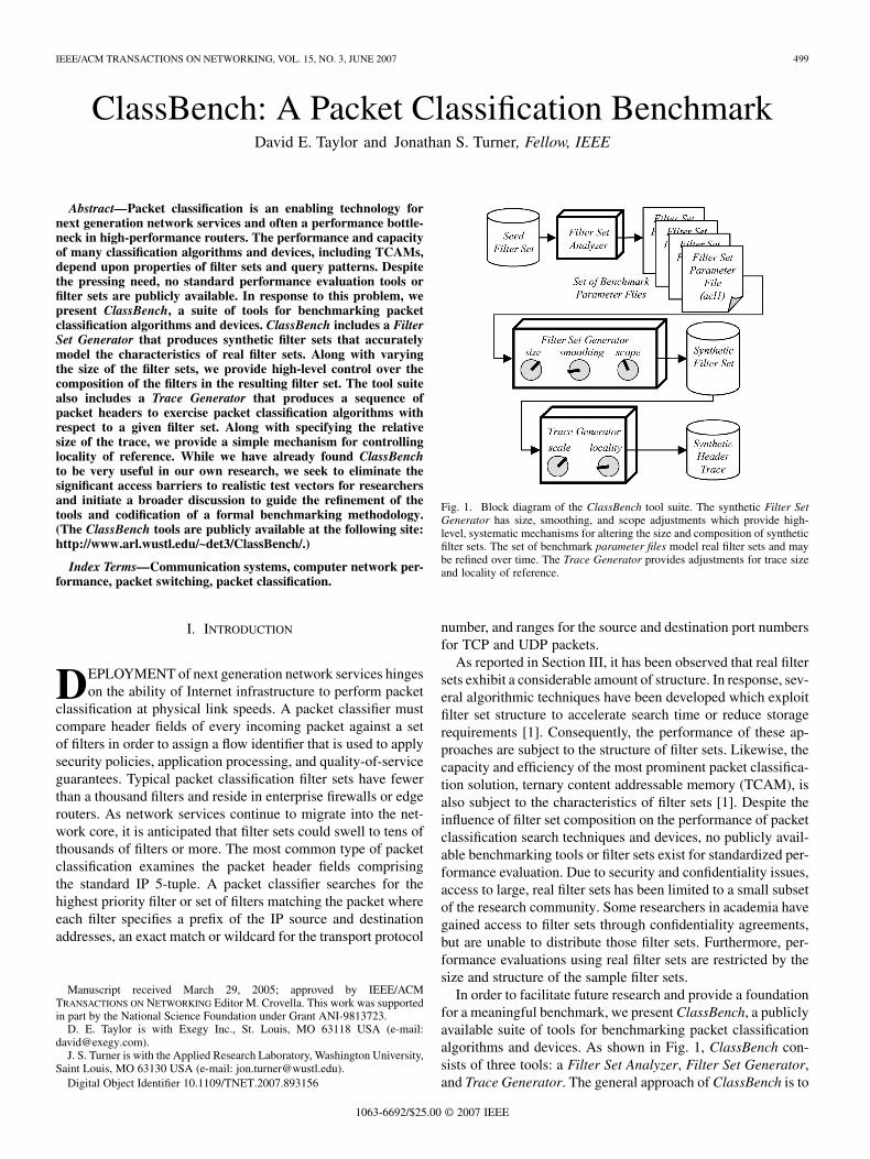
IEEE/ACM TRANSACTIONS ON NETWORKING, VOL. 15, NO. 3, JUNE 2007 499...
13
IEEE/ACM TRANSACTIONS ON NETWORKING, VOL. 15, NO. 3, JUNE 2007 499 ClassBench: A Packet Classification Benchmark David E. Taylor and Jonathan S. Turner, Fellow, IEEE Abstract—Packet classification is an enabling technology for next generation network services and often a performance bottle- neck in high-performance routers. The performance and capacity of many classification algorithms and devices, including TCAMs, depend upon properties of filter sets and query patterns. Despite the pressing need, no standard performance evaluation tools or filter sets are publicly available. In response to this problem, we present ClassBench, a suite of tools for benchmarking packet classification algorithms and devices. ClassBench includes a Filter Set Generator that produces synthetic filter sets that accurately model the characteristics of real filter sets. Along with varying the size of the filter sets, we provide high-level control over the composition of the filters in the resulting filter set. The tool suite also includes a Trace Generator that produces a sequence of packet headers to exercise packet classification algorithms with respect to a given filter set. Along with specifying the relative size of the trace, we provide a simple mechanism for controlling locality of reference. While we have already found ClassBench to be very useful in our own research, we seek to eliminate the significant access barriers to realistic test vectors for researchers and initiate a broader discussion to guide the refinement of the tools and codification of a formal benchmarking methodology. (The ClassBench tools are publicly available at the following site: http://www.arl.wustl.edu/~det3/ClassBench/.) Index Terms—Communication systems, computer network per- formance, packet switching, packet classification. I. INTRODUCTION D EPLOYMENT of next generation network services hinges on the ability of Internet infrastructure to perform packet classification at physical link speeds. A packet classifier must compare header fields of every incoming packet against a set of filters in order to assign a flow identifier that is used to apply security policies, application processing, and quality-of-service guarantees. Typical packet classification filter sets have fewer than a thousand filters and reside in enterprise firewalls or edge routers. As network services continue to migrate into the net- work core, it is anticipated that filter sets could swell to tens of thousands of filters or more. The most common type of packet classification examines the packet header fields comprising the standard IP 5-tuple. A packet classifier searches for the highest priority filter or set of filters matching the packet where each filter specifies a prefix of the IP source and destination addresses, an exact match or wildcard for the transport protocol Manuscript received March 29, 2005; approved by IEEE/ACM TRANSACTIONS ON NETWORKING Editor M. Crovella. This work was supported in part by the National Science Foundation under Grant ANI-9813723. D. E. Taylor is with Exegy Inc., St. Louis, MO 63118 USA (e-mail: [email protected]). J. S. Turner is with the Applied Research Laboratory, Washington University, Saint Louis, MO 63130 USA (e-mail: [email protected]). Digital Object Identifier 10.1109/TNET.2007.893156 Fig. 1. Block diagram of the ClassBench tool suite. The synthetic Filter Set Generator has size, smoothing, and scope adjustments which provide high- level, systematic mechanisms for altering the size and composition of synthetic filter sets. The set of benchmark parameter files model real filter sets and may be refined over time. The Trace Generator provides adjustments for trace size and locality of reference. number, and ranges for the source and destination port numbers for TCP and UDP packets. As reported in Section III, it has been observed that real filter sets exhibit a considerable amount of structure. In response, sev- eral algorithmic techniques have been developed which exploit filter set structure to accelerate search time or reduce storage requirements [1]. Consequently, the performance of these ap- proaches are subject to the structure of filter sets. Likewise, the capacity and efficiency of the most prominent packet classifica- tion solution, ternary content addressable memory (TCAM), is also subject to the characteristics of filter sets [1]. Despite the influence of filter set composition on the performance of packet classification search techniques and devices, no publicly avail- able benchmarking tools or filter sets exist for standardized per- formance evaluation. Due to security and confidentiality issues, access to large, real filter sets has been limited to a small subset of the research community. Some researchers in academia have gained access to filter sets through confidentiality agreements, but are unable to distribute those filter sets. Furthermore, per- formance evaluations using real filter sets are restricted by the size and structure of the sample filter sets. In order to facilitate future research and provide a foundation for a meaningful benchmark, we present ClassBench, a publicly available suite of tools for benchmarking packet classification algorithms and devices. As shown in Fig. 1, ClassBench con- sists of three tools: a Filter Set Analyzer, Filter Set Generator, and Trace Generator. The general approach of ClassBench is to 1063-6692/$25.00 © 2007 IEEE
Transcript of IEEE/ACM TRANSACTIONS ON NETWORKING, VOL. 15, NO. 3, JUNE 2007 499...
IEEE/ACM TRANSACTIONS ON NETWORKING, VOL. 15, NO. 3, JUNE 2007 499
ClassBench: A Packet Classification BenchmarkDavid E. Taylor and Jonathan S. Turner, Fellow, IEEE
Abstract—Packet classification is an enabling technology fornext generation network services and often a performance bottle-neck in high-performance routers. The performance and capacityof many classification algorithms and devices, including TCAMs,depend upon properties of filter sets and query patterns. Despitethe pressing need, no standard performance evaluation tools orfilter sets are publicly available. In response to this problem, wepresent ClassBench, a suite of tools for benchmarking packetclassification algorithms and devices. ClassBench includes a FilterSet Generator that produces synthetic filter sets that accuratelymodel the characteristics of real filter sets. Along with varyingthe size of the filter sets, we provide high-level control over thecomposition of the filters in the resulting filter set. The tool suitealso includes a Trace Generator that produces a sequence ofpacket headers to exercise packet classification algorithms withrespect to a given filter set. Along with specifying the relativesize of the trace, we provide a simple mechanism for controllinglocality of reference. While we have already found ClassBenchto be very useful in our own research, we seek to eliminate thesignificant access barriers to realistic test vectors for researchersand initiate a broader discussion to guide the refinement of thetools and codification of a formal benchmarking methodology.(The ClassBench tools are publicly available at the following site:http://www.arl.wustl.edu/~det3/ClassBench/.)
Index Terms—Communication systems, computer network per-formance, packet switching, packet classification.
I. INTRODUCTION
DEPLOYMENT of next generation network services hingeson the ability of Internet infrastructure to perform packet
classification at physical link speeds. A packet classifier mustcompare header fields of every incoming packet against a setof filters in order to assign a flow identifier that is used to applysecurity policies, application processing, and quality-of-serviceguarantees. Typical packet classification filter sets have fewerthan a thousand filters and reside in enterprise firewalls or edgerouters. As network services continue to migrate into the net-work core, it is anticipated that filter sets could swell to tens ofthousands of filters or more. The most common type of packetclassification examines the packet header fields comprisingthe standard IP 5-tuple. A packet classifier searches for thehighest priority filter or set of filters matching the packet whereeach filter specifies a prefix of the IP source and destinationaddresses, an exact match or wildcard for the transport protocol
Manuscript received March 29, 2005; approved by IEEE/ACMTRANSACTIONS ON NETWORKING Editor M. Crovella. This work was supportedin part by the National Science Foundation under Grant ANI-9813723.
D. E. Taylor is with Exegy Inc., St. Louis, MO 63118 USA (e-mail:[email protected]).
J. S. Turner is with the Applied Research Laboratory, Washington University,Saint Louis, MO 63130 USA (e-mail: [email protected]).
Digital Object Identifier 10.1109/TNET.2007.893156
Fig. 1. Block diagram of the ClassBench tool suite. The synthetic Filter SetGenerator has size, smoothing, and scope adjustments which provide high-level, systematic mechanisms for altering the size and composition of syntheticfilter sets. The set of benchmark parameter files model real filter sets and maybe refined over time. The Trace Generator provides adjustments for trace sizeand locality of reference.
number, and ranges for the source and destination port numbersfor TCP and UDP packets.
As reported in Section III, it has been observed that real filtersets exhibit a considerable amount of structure. In response, sev-eral algorithmic techniques have been developed which exploitfilter set structure to accelerate search time or reduce storagerequirements [1]. Consequently, the performance of these ap-proaches are subject to the structure of filter sets. Likewise, thecapacity and efficiency of the most prominent packet classifica-tion solution, ternary content addressable memory (TCAM), isalso subject to the characteristics of filter sets [1]. Despite theinfluence of filter set composition on the performance of packetclassification search techniques and devices, no publicly avail-able benchmarking tools or filter sets exist for standardized per-formance evaluation. Due to security and confidentiality issues,access to large, real filter sets has been limited to a small subsetof the research community. Some researchers in academia havegained access to filter sets through confidentiality agreements,but are unable to distribute those filter sets. Furthermore, per-formance evaluations using real filter sets are restricted by thesize and structure of the sample filter sets.
In order to facilitate future research and provide a foundationfor a meaningful benchmark, we present ClassBench, a publiclyavailable suite of tools for benchmarking packet classificationalgorithms and devices. As shown in Fig. 1, ClassBench con-sists of three tools: a Filter Set Analyzer, Filter Set Generator,and Trace Generator. The general approach of ClassBench is to
1063-6692/$25.00 © 2007 IEEE
500 IEEE/ACM TRANSACTIONS ON NETWORKING, VOL. 15, NO. 3, JUNE 2007
construct a set of benchmark parameter files that specify the rel-evant characteristics of real filter sets, generate a synthetic filterset from a chosen parameter file and a small set of high-levelinputs, and generate a sequence of packet headers to probe thesynthetic filter set using the Trace Generator. Parameter filescontain various statistics and probability distributions that guidethe generation of synthetic filter sets. The Filter Set Analyzertool extracts the relevant statistics and probability distributionsfrom a seed filter set and generates a parameter file. This pro-vides the capability to generate large synthetic filter sets whichmodel the structure of a seed filter set. In Section IV, we dis-cuss the statistics and probability distributions contained in theparameter files that drive the synthetic filter generation process.
The Filter Set Generator takes as input a parameter file anda few high-level parameters. In addition the filter set size pa-rameter, the smoothing and parameters provide high-levelcontrol over the composition of the filter set, abstracting the userfrom the low-level statistics and distributions contained in theparameter files. The smoothing adjustment provides a structuredmechanism for introducing new address aggregates which isuseful for modeling filter sets significantly larger than the filterset used to generate the parameter file. The scope adjustmentprovides a biasing mechanism to favor more or less specific fil-ters during the generation process. These adjustments and theiraffects on the resulting filter sets are discussed in Section V.Finally, the Trace Generator tool examines the synthetic filterset, then generates a sequence of packet headers to exercise thefilter set. Like the Filter Set Generator, the trace generator pro-vides adjustments for scaling the size of the trace as well as thelocality of reference of headers in the trace. These adjustmentsare described in detail in Section VI.
We highlight previous performance evaluation efforts by theresearch community as well as related benchmarking activityof the IETF in Section II. It is our hope that this work initiatesa broader discussion which will lead to refinement of the tools,compilation of a standard set of parameter files, and codificationof a formal benchmarking methodology. Its value will dependon its perceived clarity and usefulness to the interested commu-nity.
• Researchers seeking to evaluate new classification algo-rithms relative to alternative approaches and commercialproducts.
• Classification product vendors seeking to market theirproducts with convincing performance claims over com-peting products.
• Classification product customers seeking to verify andcompare classification product performance on a uniformscale.1
II. RELATED WORK
Extensive work has been done in developing benchmarks formany applications and data processing devices. Benchmarks areused extensively in the field of computer architecture to evaluatemicroprocessor performance. In the field of computer commu-nications, the Internet Engineering Task Force (IETF) has sev-
1In order to facilitate broader discussion, we make the ClassBench tools and12 parameter files publicly available at the following site: http://www.arl.wustl.edu/~det3/ClassBench/.
eral working groups exploring network performance measure-ment. Specifically, the IP Performance Metrics (IPPM) workinggroup was formed with the purpose of developing standard met-rics for Internet data delivery [2]. The Benchmarking Method-ology Working Group (BMWG) seeks to make measurementrecommendations for various internetworking technologies [3].These recommendations address metrics and performance char-acteristics as well as collection methodologies.
The BMWG specifically attacked the problem of measuringthe performance of forwarding information base (FIB) routers[4] and also produced a methodology for benchmarking fire-walls [5]. The methodology contains broad specifications suchas: the firewall should contain at least one rule for each host,tests should be run with various filter set sizes, and test trafficshould correspond to rules at the “end” of the filter set. Class-Bench complements efforts by the IETF by providing the nec-essary tools for generating test vectors with high-level controlover filter set and input trace composition. The Network Pro-cessor Forum (NPF) has also initiated a benchmarking effort [6].Currently, the NPF has produced benchmarks for switch fabricsand route lookup engines. To our knowledge, there are no cur-rent efforts by the IETF or the NPF to provide a benchmark formultiple field packet classification.
In the absence of publicly available packet filter sets, re-searchers have exerted much effort in order to generate realisticperformance tests for new algorithms. Several research groupsobtained access to real filter sets through confidentiality agree-ments. Gupta and McKeown obtained access to 40 real filtersets and extracted a number of useful statistics which havebeen widely cited [7]. Feldmann and Muthukrishnan composedfilter sets based on NetFlow packet traces from commercialnetworks [8]. Several groups have generated synthetic 2-Dfilter sets consisting of source-destination address prefix pairsby randomly selecting address prefixes from publicly availableroute tables [8]–[10]. Baboescu and Varghese also generatedsynthetic 2-D filter sets by randomly selecting prefixes frompublicly available route tables, but added refinements forcontrolling the number of zero-length prefixes (wildcards) andprefix nesting [11], [12]. A simple technique for appendingrandomly selected port ranges and protocols from real filtersets in order to generate synthetic five-dimensional filter setsis also described [11]. Baboescu and Varghese also introduceda scheme for using a sample filter set to generate a larger syn-thetic five-dimensional filter set [13]. This technique replicatesfilters by changing the IP prefixes while keeping the other fieldsunchanged. While these techniques address some aspects ofscaling filter sets in size, they lack high-level mechanisms foradjusting filter set composition which is crucial for evaluatingalgorithms that exploit filter set characteristics.
Woo provided strong motivation for a packet classificationbenchmark and initiated the effort by providing an overviewof filter characteristics for different environments (ISP PeeringRouter, ISP Core Router, Enterprise Edge Router, etc.) [14].Based on high-level characteristics, Woo generated large syn-thetic filter sets, but provided few details about how the filtersets were constructed. The technique also does not provide con-trols for varying the composition of filters within the filter set.Nonetheless, his efforts provide a good starting point for con-
TAYLOR AND TURNER: CLASSBENCH: A PACKET CLASSIFICATION BENCHMARK 501
structing a benchmark capable of modeling various applicationenvironments for packet classification. Sahasranaman and Bud-dhikot used the characteristics compiled by Woo in a compara-tive evaluation of a few packet classification techniques [15].
Stanford’s Packet Lookup and Classification Simulator(PALAC) [16] tools provide a framework for comparativeperformance evaluation of various IP lookup and packet clas-sification algorithms. The Classifier Description Language(CDL) module of PALAC gerenates a synthetic route tableor filter set based on input parameters controlling the numberof filters and the number of fields per filter. Alternatively,PALAC allows IPMA table snapshots to be used for algorithmevaluation. PALAC also includes traffic generation, statisticscollection, and classifier update modules. The ClassBench toolsuite may be used in conjunction with frameworks such asPALAC to explore the effects of filter set size and compositionon packet classifier performance.
III. ANALYSIS OF REAL FILTER SETS
Recent efforts to identify better packet classification tech-niques have focused on leveraging the characteristics of realfilter sets for faster searches. While lower bounds for the generalmulti-field searching problem have been established, observa-tions made in recent packet classification work offer enticingnew possibilities to provide significantly better performance.The focus of this section is to identify and understand the im-petus for the observed structure of filter sets and to develop met-rics and characterizations of filter set structure that aid in gener-ating synthetic filter sets. We performed a battery of analyses on12 real filter sets provided by Internet Service Providers (ISPs),a network equipment vendor, and other researchers working inthe field. The filter sets range in size from 68 to 4557 entries andutilize one of the following formats: access control list (ACL),firewall (FW), and IP chain (IPC). Due to confidentiality con-cerns, the filter sets were provided without supporting informa-tion regarding the types of systems and environments in whichthey are used. We are unable to comment on “where” in the net-work architecture the filter sets are used. Nonetheless, the fol-lowing analysis provide useful insight into the structure of realfilter sets. We observe that various useful properties hold regard-less of filter set size or format. Due to space constraints, we areunable to fully elaborate on our analysis, but a more completediscussion of this work is available in technical report form [17].
A. Understanding Filter Composition
Many of the observed characteristics of filter sets arise dueto the administrative policies that drive their construction. Themost complex packet filters typically appear in firewall and edgerouter filter sets due to the heterogeneous set of applications sup-ported in these environments. Firewalls and edge routers typi-cally implement security filters and network address translation(NAT), and they may support additional applications such asvirtual private networks (VPNs) and resource reservation. Typ-ically, these filter sets are created manually by a system admin-istrator using a standard management tool such as CiscoWorksVPN/Security Management Solution (VMS) [18] and LucentSecurity Management Server (LSMS) [19]. Such tools conform
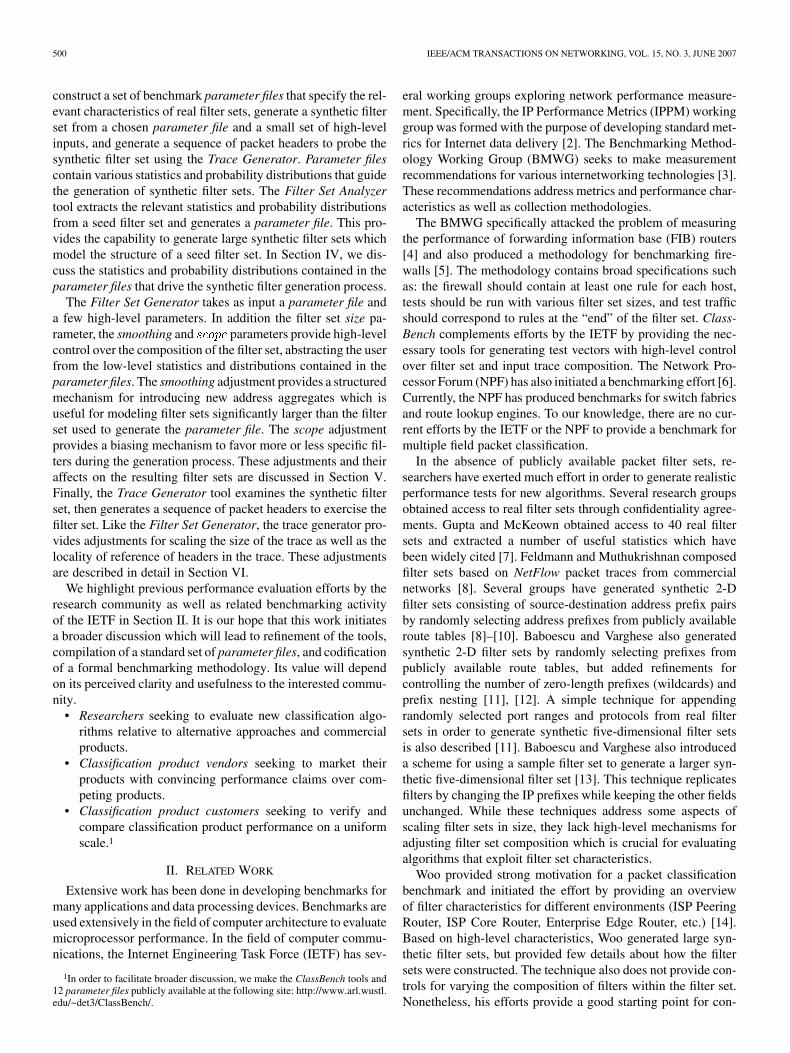
TABLE IDISTRIBUTION OF FILTERS OVER THE FIVE PORT CLASSES FOR SOURCE
AND DESTINATION PORT RANGE SPECIFICATIONS; VALUES GIVEN AS
PERCENTAGE (%) OF FILTERS IN THE FILTER SET
to a model of filter construction which views a filter as speci-fying the communicating subnets and the application or set ofapplications. Hence, we can view each filter as having two majorcomponents: an address prefix pair and an application specifica-tion. The address prefix pair identifies the communicating sub-nets by specifying a source address prefix and a destination ad-dress prefix. The application specification identifies a specificapplication session by specifying the transport protocol, sourceport number, and destination port number. A set of applicationsmay be identified by specifying ranges for the source and desti-nation port numbers.
B. Application Specifications
We analyzed the application specifications in the 12 filter setsin order to corroborate previous observations as well as extractnew, potentially useful characteristics.
1) Protocol: For each of the filter sets, we examined theunique protocol specifications and the distribution of filters overthe set of unique values. Filters specified one of nine protocolsor the wildcard. The most common protocol specification wasTCP (49%), followed by UDP (27%), the wildcard (13%), andICMP (10%). The following protocols were specified by lessthan 1% of the filters: General Routing Encapsulation (GRE),Open Shortest Path First (OSPF) Interior Gateway Protocol(IGP), Enhanced Interior Gateway Routing Protocol (EIGRP),IP Encapsulating Security Payload (ESP) for IPv6, IP Authenti-cation Header (AH) for IPv6, IP Encapsulation within IP (IPE).
2) Port Ranges: Next, we examined the port ranges specifiedby filters in the filter sets and the distribution of filters over theunique values. In order to observe trends among the various filtersets, we define five classes of port ranges:
• WC: wildcard;• HI: ephemeral user port range [1024:65535];• LO: well-known system port range [0:1023];• AR: arbitrary range;• EM: exact match.
Motivated by the allocation of port numbers, the first threeclasses represent common specifications for a port range. Thelast two classes may be viewed as partitioning the remainingspecifications based on whether or not an exact port numberis specified. We computed the distribution of filters over thefive classes for both source and destination ports for each filterset. Table I shows the combined distribution for all filter sets.We observe some interesting trends in the raw data. With rareexception, the filters in the ACL filter sets specify the wildcardfor the source port. A majority of filters in the ACL filtersspecify an exact port number for the destination port. Sourceport specifications in the other filter sets are also dominated bythe wildcard, but a considerable portion of the filters specifyan exact port number. Destination port specifications in the

502 IEEE/ACM TRANSACTIONS ON NETWORKING, VOL. 15, NO. 3, JUNE 2007
Fig. 2. Port Pair Class Matrix for TCP, filter set fw4.
other filter sets share the same trend, however the distributionbetween the wildcard and exact match is a bit more even. Onlyone filter set contained filters specifying the LO port class foreither the source or destination port range.
3) Port Pair Class: As previously discussed, the structure ofsource and destination port range pairs is a key point of interestfor both modeling real filter sets and designing efficient searchalgorithms. We can characterize this structure by defining a PortPair Class (PPC) for every combination of source and destina-tion port class. For example, WC-WC if both source and des-tination port ranges specify the wildcard, AR-LO if the sourceport range specifies an arbitrary range and the destination portrange specifies the set of well-known system ports. As shown inFig. 2, a convenient way to visualize the structure of Port PairClasses is to define a Port Pair Class Matrix where rows sharethe same source port class and columns share the same destina-tion port class. For each filter set, we examined the PPC Matrixdefined by filters specifying the same protocol. For all protocolsexcept TCP and UDP, the PPC Matrix is trivial—a single spikeat WC/WC. Fig. 2 shows the PPC Matrix defined by filters spec-ifying the TCP protocol in filter set fw4.
C. Address Prefix Pairs
A filter identifies communicating hosts or subnets by speci-fying a source and destination address prefix, or address prefixpair. The speed and efficiency of several longest prefix matchingand packet classification algorithms depend upon the number ofunique prefix lengths and the distribution of filters across thoseunique values. We find that a majority of the filter sets specifyfewer than 15 unique prefix lengths for either source or desti-nation address prefixes. The number of unique source/destina-tion prefix pair lengths is typically less than 32, which is smallrelative to the filter set size and the number of possible combi-nations, 1024. For example, the largest filter set contained 4557filters, 11 unique source address prefix lengths, 3 unique desti-nation address lengths, and 31 unique source/destination prefixpair lengths.
Fig. 3. Prefix length distribution for address prefix pairs in filter set ipc1.
Next, we examine the distribution of filters over the uniqueaddress prefix pair lengths. Note that this study is unique in thatprevious studies and models of filter sets utilized independentdistributions for source and destination address prefixes. Realfilter sets have unique prefix pair distributions that reflect thetypes of filters contained in the filter set. For example, fully spec-ified source and destination addresses dominate the distributionfor filter set ipc1 shown in Fig. 3. There are very few filters spec-ifying a 24-bit prefix for either the source or destination address,a notable difference from backbone route tables which are dom-inated by class C address prefixes (24-bit network address) andtheir aggregates. Finally, we observe that while the distributionsfor different filter sets are sufficiently different from each other amajority of the filters in the filter sets specify prefix pair lengthsaround the “edges” of the distribution. This implies that, typi-cally, one of the address prefixes is either fully specified or wild-carded.
By considering the prefix pair distribution, we characterizethe size of the communicating subnets specified by filters inthe filter set. Next, we would like to characterize the relation-ships among address prefixes and the amount of address spacecovered by the prefixes in the filter set. Consider a binary treeconstructed from the IP source address prefixes of all filters inthe filter set. From this tree, we could completely characterizethe data structure by determining a conditional branching proba-bility for each node. For example, assume that an address prefixis generated by traversing the tree starting at the root node. Ateach node, the decision to take to the 0 path or the 1 path exitingthe node depends upon the branching probability at the node.As shown in Fig. 4, is the probability that the 0 pathis chosen at level 2 given that the 1 path was chosen at level 0and the 1 path was chosen at level 1. Such a characterizationis overly complex, hence we employ suitable metrics that cap-ture the important characteristics while providing a more con-cise representation.
We begin by constructing two binary tries from the sourceand destination prefixes in the filter set. Note that there is onelevel in the tree for each possible prefix length 0 through 32for a total of 33 levels. For each level in the tree, we computethe probability that a node has one child or two children. Nodes
TAYLOR AND TURNER: CLASSBENCH: A PACKET CLASSIFICATION BENCHMARK 503
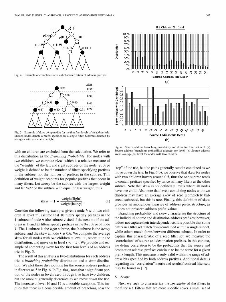
Fig. 4. Example of complete statistical characterization of address prefixes.
Fig. 5. Example of skew computation for the first four levels of an address trie.Shaded nodes denote a prefix specified by a single filter. Subtrees denoted bytriangles with associated weight.
with no children are excluded from the calculation. We refer tothis distribution as the Branching Probability. For nodes withtwo children, we compute skew, which is a relative measure ofthe “weights” of the left and right subtrees of the node. Subtreeweight is defined to be the number of filters specifying prefixesin the subtree, not the number of prefixes in the subtree. Thisdefinition of weight accounts for popular prefixes that occur inmany filters. Let heavy be the subtree with the largest weightand let light be the subtree with equal or less weight, thus
skewweight(light)
weight(heavy)(1)
Consider the following example: given a node with two chil-dren at level , assume that 10 filters specify prefixes in the1-subtree of node (the subtree visited if the next bit of the ad-dress is 1) and 25 filters specify prefixes in the 0-subtree of node
. The 1-subtree is the light subtree, the 0-subtree is the heavysubtree, and the skew at node is 0.6. We compute the averageskew for all nodes with two children at level , record it in thedistribution, and move on to level . We provide and ex-ample of computing skew for the first four levels of an addresstrie in Fig. 5.
The result of this analysis is two distributions for each addresstrie, a branching probability distribution and a skew distribu-tion. We plot these distributions for the source address prefixesin filter set acl5 in Fig. 6. In Fig. 6(a), note that a significant por-tion of the nodes in levels zero through five have two children,but the amount generally decreases as we move down the trie.The increase at level 16 and 17 is a notable exception. This im-plies that there is a considerable amount of branching near the
Fig. 6. Source address branching probability and skew for filter set acl5. (a)Source address branching probability; average per level. (b) Source addressskew; average per level for nodes with two children.
“top” of the trie, but the paths generally remain contained as wemove down the trie. In Fig. 6(b), we observe that skew for nodeswith two children hovers around 0.5, thus the one subtree tendsto contain prefixes specified by twice as many filters as the othersubtree. Note that skew is not defined at levels where all nodeshave one child. Also note that levels containing nodes with twochildren may have an average skew of zero (completely bal-anced subtrees), but this is rare. Finally, this definition of skewprovides an anonymous measure of address prefix structure, asit does not preserve address prefix values.
Branching probability and skew characterize the structure ofthe individual source and destination address prefixes; however,it does not capture their interdependence. It is possible that somefilters in a filter set match flows contained within a single subnet,while others match flows between different subnets. In order tocapture this characteristic of a seed filter set, we measure the“correlation” of source and destination prefixes. In this context,we define correlation to be the probability that the source anddestination address prefixes continue to be the same for a givenprefix length. This measure is only valid within the range of ad-dress bits specified by both address prefixes. Additional detailsregarding the “correlation” metric and results from real filter setsmay be found in [17].
D. Scope
Next we seek to characterize the specificity of the filters inthe filter set. Filters that are more specific cover a small set of

504 IEEE/ACM TRANSACTIONS ON NETWORKING, VOL. 15, NO. 3, JUNE 2007
possible packet headers while filters that are less specific covera large set of possible packet headers. The number of possiblepacket headers covered by a filter is characterized by its tuplespecification. To be specific, we consider the standard 5-tupleas a vector containing the following fields:
• : source address prefix length ;• : destination address prefix length ;• : source port range width, the number of port numbers
covered by the range ;• : destination port range width, the number of port num-
bers covered by the range ;• : protocol specification, Boolean value denoting
whether or not a protocol is specified [0, 1].We define a new metric, scope, to be the logarithmic measureof the number of possible packet headers covered by the filter.Using the definition above, we define a filter’s 5-tuple scope asfollows:
scope
(2)
Thus, scope is a measure of filter specificity on a scale from 0to 104. The average 5-tuple scope for our 12 filter sets rangesfrom 56 to 24. We note that filters in the ACL filter sets tend tohave narrower scope, while filters in the FW filter sets tend tohave wider scope.
E. Additional Fields
An examination of real filter sets reveals that additional fieldsbeyond the standard 5-tuple are relevant. In 10 of the 12 filtersets that we studied, filters contain matches on TCP flags orICMP type numbers. In most filter sets, a small percentage ofthe filters specify a nonwildcard value for the flags, typicallyless then two percent. There are notable exceptions, as approxi-mately half the filters in filter set ipc1 contain nonwildcard flags.We argue that new services and administrative policies will de-mand that packet classification techniques scale to support ad-ditional fields beyond the standard 5-tuple. Matches on ICMPtype number and other higher-level header fields are likely to beexact matches. There may be other types of matches that morenaturally suit the application, such as arbitrary bit masks on TCPflags.
IV. PARAMETER FILES
Given a real filter set, the Filter Set Analyzer generates a pa-rameter file that contains statistics and probability distributionsthat allow the Filter Set Generator to produce a synthetic filterset that retains the relevant characteristics of the original filterset. We chose the statistics and distributions to include in the pa-rameter file based on thorough analysis of 12 real filter sets andseveral iterations of the Filter Set Generator design. Note thatparameter files also provide complete anonymity of addressesin the original filter set. By reducing confidentiality concerns,
we seek to remove the significant access barriers to realistic testvectors for researchers and promote the development of a bench-mark set of parameter files. There still exists a need for a largesample space of real filter sets from various application environ-ments. We have generated a set of 12 parameter files which arepublicly available along with the ClassBench tool suite.
Parameter files include the following entries.2
• Protocol specifications and the distribution of filters overthose values.
• Port Pair Class Matrix for each unique protocol specifica-tion in the filter set
• Flags specifications for each protocol and a distribution offilters over those values.
• Arbitrary port range specifications and a distribution offilters over those values for both the source and destinationport fields.
• Exact port number specifications and a distribution of fil-ters over those values for both the source and destinationport fields.
• Prefix pair length distribution for each Port Pair Class Ma-trix.
• Address prefix branching and skew distributions for bothsource and destination address prefixes.
• Address prefix correlation distribution.• Prefix nesting thresholds for both source and destination
address prefixes.Parameter files represent prefix pair length distributions using
a combination of a total prefix length distribution and sourceprefix length distributions for each specified total length3 asshown in Fig. 7. The total prefix length is simply the sum ofthe prefix lengths for the source and destination address pre-fixes. As we will demonstrate in Section V-B, modeling the totalprefix length distribution allows us to easily bias the generationof more or less specific filters based on the scope input param-eter. The source prefix length distributions associated with eachspecified total length allow us to model the prefix pair lengthdistribution, as the destination prefix length is simply the differ-ence of the total length and the source length.
The number of unique address prefixes that match a givenpacket is an important property of real filter sets and is oftenreferred to as prefix nesting. We found that if the Filter Set Gen-erator is ignorant of this property, it is likely to create filter setswith significantly higher prefix nesting, especially when the syn-thetic filter set is larger than the filter set used to generate theparameter file. Given that prefix nesting remains relatively con-stant for filter sets of various sizes, we place a limit on the prefixnesting during the filter generation process. The Filter Set Ana-lyzer computes the maximum prefix nesting for both the sourceand destination address prefixes in the filter set and records thesestatistics in the parameter file. The Filter Set Generator retainsthese prefix nesting properties in the synthetic filter set, regard-less of size. We discuss the process of generating address pre-fixes and retaining prefix nesting properties in Section V.
2We avoid an exhaustive discussion of parameter file contents and format de-tails; interested readers and potential users of ClassBench may find a discussionof parameter file format in the documentation provided with the tools.
3We do not need to store a source prefix distribution for total prefix lengthsthat are not specified by filters in the filter set.

TAYLOR AND TURNER: CLASSBENCH: A PACKET CLASSIFICATION BENCHMARK 505
Fig. 7. Parameter files represent prefix pair length distributions using a combination of a total prefix length distribution and source prefix length distributions foreach nonzero total length.
V. SYNTHETIC FILTER SET GENERATION
The Filter Set Generator is the cornerstone of the ClassBenchtool suite. Perhaps the most succinct way to describe the syn-thetic filter set generation process is to walk through the pseu-docode shown in Fig. 8. The first step in the filter generationprocess is to read the statistics and distributions from the pa-rameter file. Next, we get the four high-level input parameters:
• size: target size for the synthetic filter set;• smoothing: controls the number of new address aggregates
(prefix lengths);• port scope: biases the tool to generate more or less specific
port range pairs;• address scope: biases the tool to generate more or less spe-
cific address prefix pairs.We refer to the size parameter as a “target” size because the gen-erated filter set may have fewer filters. This is due to the fact thatit is possible for the Filter Set Generator to produce a filter setcontaining redundant filters, thus the final step in the processremoves the redundant filters. The generation of redundant fil-ters stems from the way the tool assigns source and destinationaddress prefixes that preserve the properties specified in the pa-rameter file. This process will be described in more detail in amoment.
Before we begin the generation process, we apply thesmoothing adjustment to the prefix pair length distributions4
(lines 6–10). In order to apply the smoothing adjustment, wemust iterate over all Port Pair Classes (line 7), apply the adjust-ment to each total prefix length distribution (line 8) and iterateover all total prefix lengths (line 9), and apply the adjustmentto each source prefix length distribution associated with thetotal prefix length (line 10). We discuss this adjustment and itseffects on the generated filter set in Section V-A.
The next set of steps (lines 12–27) generate a partial filterfor each entry in the Filters array. Essentially, we assign allfilter fields except the address prefix values. Note that the prefix
4Note that the scope adjustments do not add any new prefix lengths to thedistributions. It only changes the likelihood that longer or shorter prefix lengthsin the distribution are chosen.
lengths for both source and destination address are assigned.The reason for this approach will become clear when we dis-cuss the assignment of address prefix values in a moment. Thefirst step in generating a partial filter is to select a protocol fromthe Protocols distribution (line 14) using a uniform randomvariable, (line 13). We chose to select the protocol first be-cause we found that the protocol specification dictates the struc-ture of the other filter fields. Next, we select the protocol flags5
from the Flags distribution associated with the chosen pro-tocol (line 16).
After choosing the protocol and flags, we select a Port PairClass, , from the Port Pair Class Matrix, PPCMatrix, as-sociated with the chosen protocol (line 18). Note that the se-lection of the is performed with a random variable that isbiased by the port scope parameter (line 17). This adjustment al-lows the user to bias the Filter Set Generator to produce a filterset with more or less specific s, where WC-WC (both portranges wildcarded) is the least specific and EM-EM (both portranges specify an exact match port number) is the most specific.We discuss this adjustment and its effects on the generated filterset in Section V-B. Given the , we can select the source anddestination port ranges from their respective port range distri-butions associated with each port class (lines 20 and 22). Notethat the distributions for port classes WC, HI, and LO are trivialas they define single ranges.
Selecting the address prefix pair lengths is the last step ingenerating a partial filter. We select a total prefix pair lengthfrom the distribution associated with the chosen (line 24)using a random variable biased by the address scope parameter(line 23). We select a source prefix length from the distributionassociated with the chosen and total length (line 26) usinga uniform random variable (line 25). Finally, we calculate thedestination address prefix length using the chosen total lengthand source address prefix length (line 27).
After we generate all the partial filters, we must assign thesource and destination address prefix values. The AssignSA
5Note that the protocol flags field is typically the wildcard unless the chosenprotocol is TCP or ICMP.
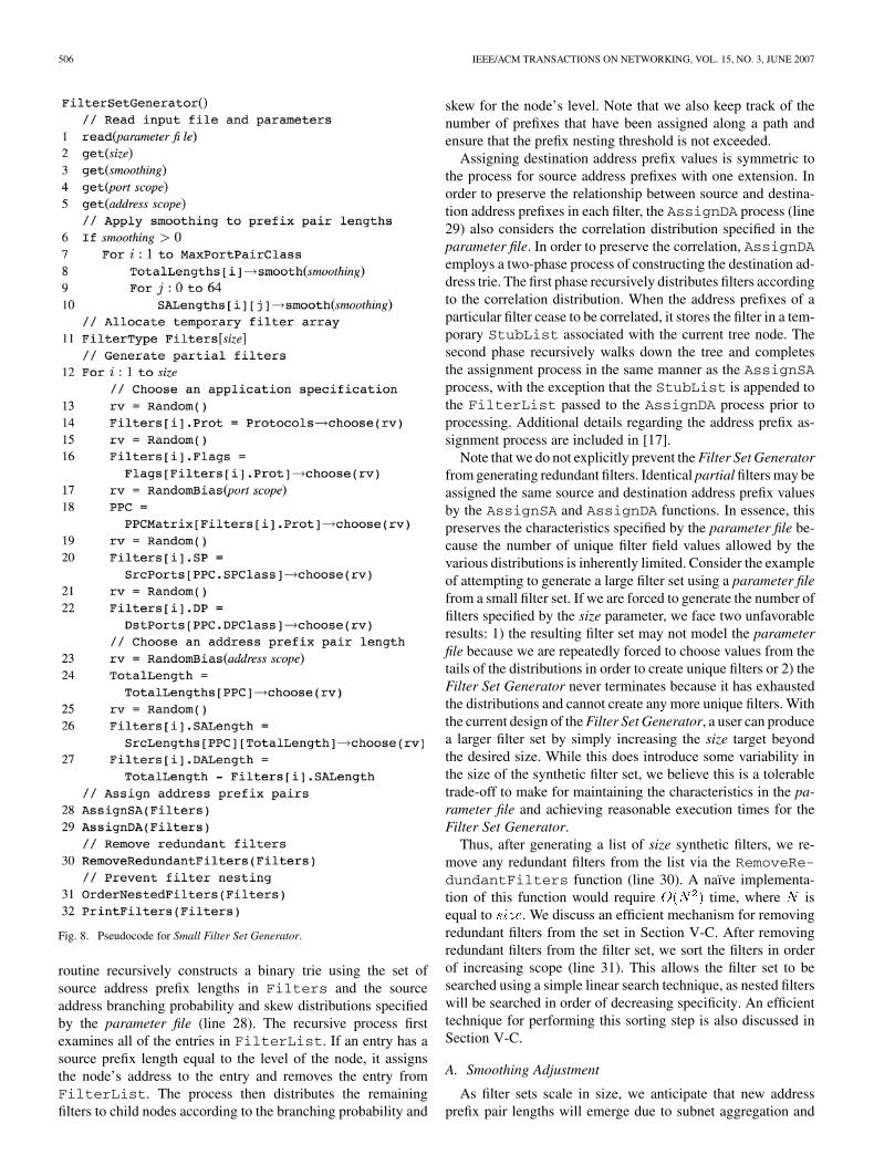
506 IEEE/ACM TRANSACTIONS ON NETWORKING, VOL. 15, NO. 3, JUNE 2007
Fig. 8. Pseudocode for Small Filter Set Generator.
routine recursively constructs a binary trie using the set ofsource address prefix lengths in Filters and the sourceaddress branching probability and skew distributions specifiedby the parameter file (line 28). The recursive process firstexamines all of the entries in FilterList. If an entry has asource prefix length equal to the level of the node, it assignsthe node’s address to the entry and removes the entry fromFilterList. The process then distributes the remainingfilters to child nodes according to the branching probability and
skew for the node’s level. Note that we also keep track of thenumber of prefixes that have been assigned along a path andensure that the prefix nesting threshold is not exceeded.
Assigning destination address prefix values is symmetric tothe process for source address prefixes with one extension. Inorder to preserve the relationship between source and destina-tion address prefixes in each filter, the AssignDA process (line29) also considers the correlation distribution specified in theparameter file. In order to preserve the correlation, AssignDAemploys a two-phase process of constructing the destination ad-dress trie. The first phase recursively distributes filters accordingto the correlation distribution. When the address prefixes of aparticular filter cease to be correlated, it stores the filter in a tem-porary StubList associated with the current tree node. Thesecond phase recursively walks down the tree and completesthe assignment process in the same manner as the AssignSAprocess, with the exception that the StubList is appended tothe FilterList passed to the AssignDA process prior toprocessing. Additional details regarding the address prefix as-signment process are included in [17].
Note that we do not explicitly prevent the Filter Set Generatorfrom generating redundant filters. Identical partial filters may beassigned the same source and destination address prefix valuesby the AssignSA and AssignDA functions. In essence, thispreserves the characteristics specified by the parameter file be-cause the number of unique filter field values allowed by thevarious distributions is inherently limited. Consider the exampleof attempting to generate a large filter set using a parameter filefrom a small filter set. If we are forced to generate the number offilters specified by the size parameter, we face two unfavorableresults: 1) the resulting filter set may not model the parameterfile because we are repeatedly forced to choose values from thetails of the distributions in order to create unique filters or 2) theFilter Set Generator never terminates because it has exhaustedthe distributions and cannot create any more unique filters. Withthe current design of the Filter Set Generator, a user can producea larger filter set by simply increasing the size target beyondthe desired size. While this does introduce some variability inthe size of the synthetic filter set, we believe this is a tolerabletrade-off to make for maintaining the characteristics in the pa-rameter file and achieving reasonable execution times for theFilter Set Generator.
Thus, after generating a list of size synthetic filters, we re-move any redundant filters from the list via the RemoveRe-dundantFilters function (line 30). A naïve implementa-tion of this function would require time, where isequal to . We discuss an efficient mechanism for removingredundant filters from the set in Section V-C. After removingredundant filters from the filter set, we sort the filters in orderof increasing scope (line 31). This allows the filter set to besearched using a simple linear search technique, as nested filterswill be searched in order of decreasing specificity. An efficienttechnique for performing this sorting step is also discussed inSection V-C.
A. Smoothing Adjustment
As filter sets scale in size, we anticipate that new addressprefix pair lengths will emerge due to subnet aggregation and
TAYLOR AND TURNER: CLASSBENCH: A PACKET CLASSIFICATION BENCHMARK 507
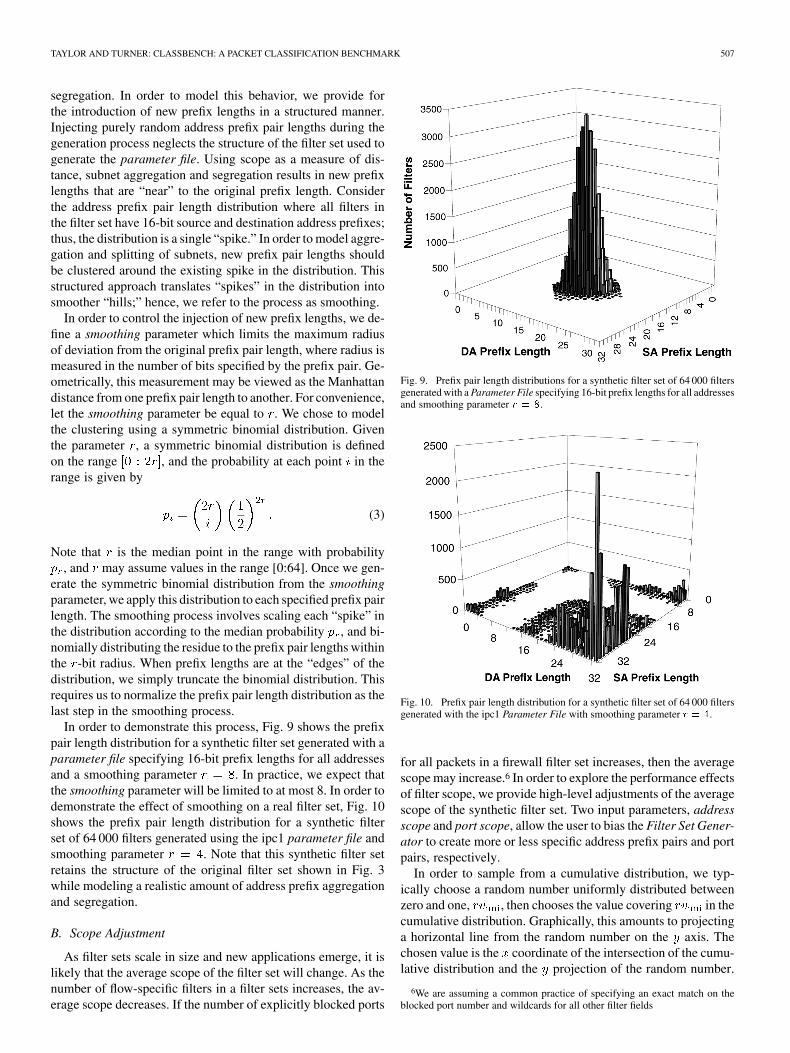
segregation. In order to model this behavior, we provide forthe introduction of new prefix lengths in a structured manner.Injecting purely random address prefix pair lengths during thegeneration process neglects the structure of the filter set used togenerate the parameter file. Using scope as a measure of dis-tance, subnet aggregation and segregation results in new prefixlengths that are “near” to the original prefix length. Considerthe address prefix pair length distribution where all filters inthe filter set have 16-bit source and destination address prefixes;thus, the distribution is a single “spike.” In order to model aggre-gation and splitting of subnets, new prefix pair lengths shouldbe clustered around the existing spike in the distribution. Thisstructured approach translates “spikes” in the distribution intosmoother “hills;” hence, we refer to the process as smoothing.
In order to control the injection of new prefix lengths, we de-fine a smoothing parameter which limits the maximum radiusof deviation from the original prefix pair length, where radius ismeasured in the number of bits specified by the prefix pair. Ge-ometrically, this measurement may be viewed as the Manhattandistance from one prefix pair length to another. For convenience,let the smoothing parameter be equal to . We chose to modelthe clustering using a symmetric binomial distribution. Giventhe parameter , a symmetric binomial distribution is definedon the range , and the probability at each point in therange is given by
(3)
Note that is the median point in the range with probability, and may assume values in the range [0:64]. Once we gen-
erate the symmetric binomial distribution from the smoothingparameter, we apply this distribution to each specified prefix pairlength. The smoothing process involves scaling each “spike” inthe distribution according to the median probability , and bi-nomially distributing the residue to the prefix pair lengths withinthe -bit radius. When prefix lengths are at the “edges” of thedistribution, we simply truncate the binomial distribution. Thisrequires us to normalize the prefix pair length distribution as thelast step in the smoothing process.
In order to demonstrate this process, Fig. 9 shows the prefixpair length distribution for a synthetic filter set generated with aparameter file specifying 16-bit prefix lengths for all addressesand a smoothing parameter . In practice, we expect thatthe smoothing parameter will be limited to at most 8. In order todemonstrate the effect of smoothing on a real filter set, Fig. 10shows the prefix pair length distribution for a synthetic filterset of 64 000 filters generated using the ipc1 parameter file andsmoothing parameter . Note that this synthetic filter setretains the structure of the original filter set shown in Fig. 3while modeling a realistic amount of address prefix aggregationand segregation.
B. Scope Adjustment
As filter sets scale in size and new applications emerge, it islikely that the average scope of the filter set will change. As thenumber of flow-specific filters in a filter sets increases, the av-erage scope decreases. If the number of explicitly blocked ports
Fig. 9. Prefix pair length distributions for a synthetic filter set of 64 000 filtersgenerated with a Parameter File specifying 16-bit prefix lengths for all addressesand smoothing parameter r = 8.
Fig. 10. Prefix pair length distribution for a synthetic filter set of 64 000 filtersgenerated with the ipc1 Parameter File with smoothing parameter r = 4.
for all packets in a firewall filter set increases, then the averagescope may increase.6 In order to explore the performance effectsof filter scope, we provide high-level adjustments of the averagescope of the synthetic filter set. Two input parameters, addressscope and port scope, allow the user to bias the Filter Set Gener-ator to create more or less specific address prefix pairs and portpairs, respectively.
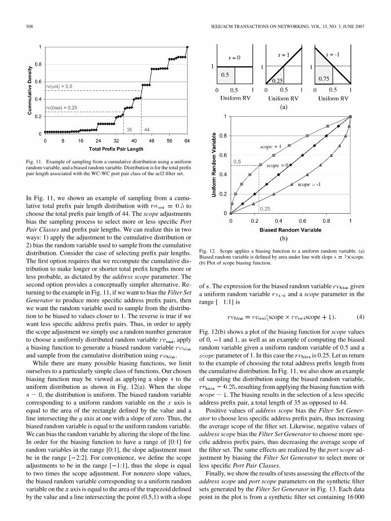
In order to sample from a cumulative distribution, we typ-ically choose a random number uniformly distributed betweenzero and one, , then chooses the value covering in thecumulative distribution. Graphically, this amounts to projectinga horizontal line from the random number on the axis. Thechosen value is the coordinate of the intersection of the cumu-lative distribution and the projection of the random number.
6We are assuming a common practice of specifying an exact match on theblocked port number and wildcards for all other filter fields
508 IEEE/ACM TRANSACTIONS ON NETWORKING, VOL. 15, NO. 3, JUNE 2007
Fig. 11. Example of sampling from a cumulative distribution using a uniformrandom variable, and a biased random variable. Distribution is for the total prefixpair length associated with the WC-WC port pair class of the acl2 filter set.
In Fig. 11, we shown an example of sampling from a cumu-lative total prefix pair length distribution with tochoose the total prefix pair length of 44. The scope adjustmentsbias the sampling process to select more or less specific PortPair Classes and prefix pair lengths. We can realize this in twoways: 1) apply the adjustment to the cumulative distribution or2) bias the random variable used to sample from the cumulativedistribution. Consider the case of selecting prefix pair lengths.The first option requires that we recompute the cumulative dis-tribution to make longer or shorter total prefix lengths more orless probable, as dictated by the address scope parameter. Thesecond option provides a conceptually simpler alternative. Re-turning to the example in Fig. 11, if we want to bias the Filter SetGenerator to produce more specific address prefix pairs, thenwe want the random variable used to sample from the distribu-tion to be biased to values closer to 1. The reverse is true if wewant less specific address prefix pairs. Thus, in order to applythe scope adjustment we simply use a random number generatorto choose a uniformly distributed random variable , applya biasing function to generate a biased random variableand sample from the cumulative distribution using .
While there are many possible biasing functions, we limitourselves to a particularly simple class of functions. Our chosenbiasing function may be viewed as applying a slope to theuniform distribution as shown in Fig. 12(a). When the slope
, the distribution is uniform. The biased random variablecorresponding to a uniform random variable on the axis isequal to the area of the rectangle defined by the value and aline intersecting the axis at one with a slope of zero. Thus, thebiased random variable is equal to the uniform random variable.We can bias the random variable by altering the slope of the line.In order for the biasing function to have a range of [0:1] forrandom variables in the range [0:1], the slope adjustment mustbe in the range [ 2:2]. For convenience, we define the scopeadjustments to be in the range [ 1:1], thus the slope is equalto two times the scope adjustment. For nonzero slope values,the biased random variable corresponding to a uniform randomvariable on the axis is equal to the area of the trapezoid definedby the value and a line intersecting the point (0.5,1) with a slope
Fig. 12. Scope applies a biasing function to a uniform random variable. (a)Biased random variable is defined by area under line with slope s = 2�scope.(b) Plot of scope biasing function.
of . The expression for the biased random variable givena uniform random variable and a scope parameter in therange [ 1:1] is
scope scope (4)
Fig. 12(b) shows a plot of the biasing function for scope valuesof 0, 1 and 1, as well as an example of computing the biasedrandom variable given a uniform random variable of 0.5 and a
parameter of 1. In this case the is 0.25. Let us returnto the example of choosing the total address prefix length fromthe cumulative distribution. In Fig. 11, we also show an exampleof sampling the distribution using the biased random variable,
, resulting from applying the biasing function with. The biasing results in the selection of a less specific
address prefix pair, a total length of 35 as opposed to 44.Positive values of address scope bias the Filter Set Gener-
ator to choose less specific address prefix pairs, thus increasingthe average scope of the filter set. Likewise, negative values ofaddress scope bias the Filter Set Generator to choose more spe-cific address prefix pairs, thus decreasing the average scope ofthe filter set. The same effects are realized by the port scope ad-justment by biasing the Filter Set Generator to select more orless specific Port Pair Classes.
Finally, we show the results of tests assessing the effects of theaddress scope and port scope parameters on the synthetic filtersets generated by the Filter Set Generator in Fig. 13. Each datapoint in the plot is from a synthetic filter set containing 16 000

TAYLOR AND TURNER: CLASSBENCH: A PACKET CLASSIFICATION BENCHMARK 509
Fig. 13. Average scope of synthetic filter sets consisting of 16 000 filters gen-erated with parameter files extracted from filter sets acl3, fw5, and ipc1, andvarious values of the scope parameters.
filters generated from a parameter file from filter sets acl3, fw5,or ipc1. For these tests, both scope parameters were set to thesame value. Over their range of values, the scope parametersalter the average filter scope by 6– 7.5. We also measuredthe individual effects of the address scope and port scope pa-rameters. Over its range of values, the address scope alters theaverage address pair scope by 4– 6. Over its range of values,the port scope alters the average port pair scope by 1.5– 2.5.These scope adjustments provide a convenient high-level mech-anism for exploring the effects of filter specificity on the perfor-mance of packet classification algorithms and devices.
C. Filter Redundancy and Priority
The final steps in synthetic filter set generation are removingredundant filters and ordering the remaining filters in order ofincreasing scope. The removal of redundant filters may be re-alized by simply comparing each filter against all other filtersin the set; however, this naïve implementation requirestime. Such an approach makes execution times of the Filter SetGenerator prohibitively long for filter sets with more than a fewthousand filters. In order to accelerate this process, we first sortthe filters into sets according to their tuple specification. We per-form this sorting efficiently by constructing a binary search treeof tuple set pointers, using the scope of the tuple as the key forthe node. When adding a filter to a tuple set, we search the set forredundant filters. If no redundant filters exist in the set, then weadd the filter to the set. If a redundant filter exists in the set, wediscard the filter. The time complexity of this search techniquedepends on the number of tuples created by filters in the filterset and the distribution of filters across the tuples. In practice,we find that this technique provides acceptable performance.
In order to support the traditional linear search technique,filter priority is often inferred by placement in an ordered list.In such cases, the first matching filter is the best matching filter.This arrangement could obviate a filter if a less specific filter
occupies a higher position in the list. To prevent this,we order the filters in the synthetic filter set according to scope,
Fig. 14. Pseudocode for Trace Generator.
where filters with minimum scope occur first. The binary searchtree of tuple set pointers makes this ordering task simple. Recallthat we use scope as the node key. Thus, we simply perform anin-order walk of the binary search tree, appending the filters ineach tuple set to the output list of filters.
VI. TRACE GENERATION
When benchmarking a particular packet classification algo-rithm or device, many of the metrics of interest such as storageefficiency and maximum decision tree depth may be garneredusing the synthetic filter sets generated by the Filter Set Gen-erator. In order to evaluate the throughput of techniques em-ploying caching or the power consumption of various devicesunder load, we must exercise the algorithm or device using a se-quence of synthetic packet headers. The Trace Generator pro-duces a list of synthetic packet headers that probe filters in agiven filter set. Note that we do not want to generate randompacket headers. Rather, we want to ensure that a packet headeris covered by at least one filter in the FilterSet in order to ex-ercise the packet classifier and avoid default filter matches. Weexperimented with a number of techniques to generate syntheticheaders. One possibility is to compute all the -dimensionalpolyhedra defined by the intersections of the filters in the filterset, then choose a point in the -dimensional space coveredby the polyhedra. The point defines a packet header. The best-matching filter for the packet header is simply the highest pri-ority filter associated with the polyhedra. If we generate at leastone header corresponding to each polyhedra, we fully exercisethe filter set. The number of polyhedra defined by filter inter-sections grows exponentially, and thus fully exercising the filterset quickly becomes intractable. As a result, we chose a methodthat partially exercises the filter set and allows the user to varythe size and composition of the headers in the trace using high-level input parameters. These parameters control the scale ofthe header trace relative to the filter set, as well as the locality ofreference in the sequence of headers. As we did with the FilterSet Generator, we discuss the Trace Generator using the pseu-docode shown in Fig. 14.

510 IEEE/ACM TRANSACTIONS ON NETWORKING, VOL. 15, NO. 3, JUNE 2007
We begin by reading the FilterSet (line 1) and getting theinput parameters scale, ParetoA, and ParetoB (lines 2–4). Thescale parameter is used to set a threshold for the size of the listof headers relative to the size of the FilterSet (line 5). In thiscontext, scale specifies the ratio of the number of headers in thetrace to the number of filters in the filter set. The next set ofsteps continue to generate synthetic headers as long as the sizeof Headers does not exceed the Threshold defined by theproduct of scale and the number filters in FilterSet.
Each iteration of the header generation loop begins by se-lecting a random filter in the FilterSet (line 8). Next, we mustchoose a packet header covered by the filter. In the interest ofexercising priority resolution mechanisms and providing con-servative performance estimates for algorithms relying on filteroverlap properties, we would like to choose headers matching alarge number of filters. In the course of our analyses, we foundthe number of overlapping filters is large for packet headersrepresenting the “corners” of filters. Each field of a filter coversa range of values. Choosing a packet header correspondingto a “corner” translates to choosing a value for each headerfield from one of the extrema of the range specified by eachfilter field. The RandomCorner function chooses a random“corner” of the filter identified by RandFilt and stores theheader in NewHeader.
The last steps in the header generation loop append a variablenumber of copies of NewHeader to the trace. The number ofcopies, Copies, is chosen by sampling from a Pareto distri-bution controlled by the input parameters, ParetoA and ParetoB(line 10). In doing so, we provide a simple control point for thelocality of reference in the header trace. The Pareto distribu-tion7 is one of the heavy-tailed distributions commonly used tomodel the burst size of Internet traffic flows as well as the filesize distribution for traffic using the TCP protocol [20]. For con-venience, let ParetoA and ParetoB. The probability den-sity function for the Pareto distribution may be expressed as
(5)
where the cumulative distribution is
(6)
The Pareto distribution has a mean of
(7)
Expressed in this way, is typically called the shape parameterand is typically called the scale parameter, as the distributionis defined on values in the interval . The following aresome examples of how the Pareto parameters are used to controllocality of reference.
• Low locality of reference, short tail: ( , ) mostheaders will be inserted once.
• Low locality of reference, long tail: ( , ) manyheaders will be inserted once, but some could be insertedover 20 times.
7The Pareto distribution, a power law distribution named after the Italianeconomist Vilfredo Pareto, is also known as the Bradford distribution.
• High locality of reference, short tail: ( , ) mostheaders will be inserted four times.
Once the size of the trace exceeds the threshold, the header gen-eration loop terminates. Note that a large burst near the end ofthe process will cause the trace to be larger than Threshold.After generating the list of headers, we write the trace to anoutput file (line 13).
VII. DISCUSSION
We have already found ClassBench to be tremendously valu-able in our own research [21]–[23]. The ClassBench tools havealso been used in a graduate level computer architecture course.Student groups used the tools to evaluate the performance ofvarious packet classification algorithms [7], [21], [25], [26] im-plemented on an Intel IXP network processor [24].8
ACKNOWLEDGMENT
The authors would like to thank E. Spitznagel for contributinghis insight to countless discussions on packet classification andassisting in the debugging of the ClassBench tools. They alsowould like to thank V. Srinivasan and W. Eatherton for makingreal filter sets available for study.
REFERENCES
[1] D. E. Taylor, “Survey and taxonomy of packet classification tech-niques,” ACM Comput. Surv., vol. 37, no. 5, pp. 238–275, Sep. 2005.
[2] V. Paxson, G. Almes, J. Mahdavi, and M. Mathis, “Framework for IPperformance metrics,” RFC 2330, May 1998.
[3] S. Bradner and J. McQuaid, “Benchmarking methodology for networkinterconnect devices,” RFC 2544, Mar. 1999.
[4] G. Trotter, “Methodology for forwarding information base (FIB) basedrouter performance,” Internet Draft, Jan. 2002.
[5] B. Hickman, D. Newman, S. Tadjudin, and T. Martin, “Benchmarkingmethodology for firewall performance,” RFC 3511, Apr. 2003.
[6] P. Chandra, F. Hady, and S. Y. Lim, “Framework for benchmarkingnetwork processors,” in Proc. Netw. Process. Forum, 2002.
[7] P. Gupta and N. McKeown, “Packet classification on multiple fields,”in Proc. ACM SIGCOMM, Aug. 1999, pp. 147–160.
[8] A. Feldmann and S. Muthukrishnan, “Tradeoffs for packet classifica-tion,” in Proc. IEEE INFOCOM, Mar. 2000, pp. 1193–1202.
[9] P. Gupta and N. McKeown, “Packet classification using hierarchicalintelligent cuttings,” in Proc. Hot Interconnects VII, Aug. 1999, pp.27–31.
[10] P. Warkhede, S. Suri, and G. Varghese, “Fast packet classificationfor 2-D conflict-free filters,” in Proc. IEEE INFOCOM, 2001, pp.1434–1443.
[11] F. Baboescu and G. Varghese, “Scalable packet classification,” in Proc.ACM SIGCOMM, Aug. 2001, pp. 199–210.
[12] F. Baboescu and G. Varghese, “Fast and scalable conflict detection forpacket classifiers,” in Proc. IEEE ICNP, 2002, pp. 270–279.
[13] F. Baboescu, S. Singh, and G. Varghese, “Packet classification for corerouters: Is there an alternative to CAMs?,” in Proc. IEEE INFOCOM,2003, pp. 53–63.
[14] T. Y. C. Woo, “A modular approach to packet classification: Al-gorithms and results,” in Proc. IEEE INFOCOM, Mar. 2000, pp.1213–1222.
[15] V. Sahasranaman and M. Buddhikot, “Comparative evaluation ofsoftware implementations of layer 4 packet classification schemes,” inProc. IEEE Int. Conf. Netw. Protocols, 2001, pp. 220–228.
[16] J. Balkman and P. Gupta, PALAC: Packet Lookup and ClassificationSimulator, User’s Manual, ver. 4, Rev. 1 Oct. 2000.
[17] D. E. Taylor and J. S. Turner, “ClassBench: A packet classificationbenchmark,” Dept. Comp. Sci. Eng., Washington Univ., St. Louis,Tech. Rep. WUCSE-2004-28, May 2004.
[18] Cisco, CiscoWorks VPN/Security Management Solution, Cisco Sys-tems, Inc., 2004, Tech. Rep..
8 The ClassBench tools and 12 parameter files are publicly available at thefollowing site: http://www.arl.wustl.edu/~det3/ClassBench/.

TAYLOR AND TURNER: CLASSBENCH: A PACKET CLASSIFICATION BENCHMARK 511
[19] Lucent, Lucent Security Management Server: Security, VPN, and QoSManagement Solution, Lucent Technologies Inc., 2004, Tech. Rep..
[20] K. Park, G. Kim, and M. Crovella, “On the effect of traffic self-simi-larity on network performance,” in Proc. 1997 SPIE Int. Conf. Perform.Contr. Netw. Syst., pp. 989–996.
[21] D. E. Taylor and J. S. Turner, “Scalable packet classification using dis-tributed crossproducting of field labels,” in Proc. IEEE INFOCOM,Mar. 2005, pp. 269–280.
[22] E. Spitznagel, D. Taylor, and J. Turner, “Packet classification usingextended TCAMs,” in Proc. IEEE ICNP, 2003, pp. 120–131.
[23] D. E. Taylor and E. W. Spitznagel, “On using content addressablememory for packet classification,” Dept. Comp. Sci. Eng., WashingtonUniv., Saint Louis, Tech. Rep. WUCSE-2005-9, Mar. 2005.
[24] Intel Corp., IXP2400 Network Processor, Product Brief, Tech. Rep.,2002.
[25] S. Singh, F. Baboescu, G. Varghese, and J. Wang, “Packet classificationusing multidimensional cutting,” in Proc. ACM SIGCOMM, 2003, pp.213–224.
[26] V. Srinivasan, S. Suri, and G. Varghese, “Packet classification usingtuple space search,” in Proc. ACM SIGCOMM, 1999, pp. 135–146.
David E. Taylor received the B.S. and M.S. degreesin electrical and computer engineering in 1998 and2002, respectively, and the D.Sc. degree in computerengineering in 2004, all from Washington University,St. Louis, MO.
He is a System Architect and the Director ofHardware Engineering at Exegy Inc., St. Louis,MO, where his primary focus is the developmentof high-performance hybrid computing systemsfor government intelligence and financial servicesapplications. Prior to joining Exegy, he was a
Visiting Assistant Professor in the Department of Computer Science and
Engineering, Washington University, where he was also actively involvedin computer communications research at the Applied Research Laboratory.His research interests include the design and analysis of scalable searchingalgorithms and architectures, IP lookup and packet classification algorithms,high-performance reconfigurable hardware systems, programmable routers,and network processors.
Jonathan S. Turner (M’77–SM’88–F’90) receivedthe M.S. and Ph.D. degrees in computer science fromNorthwestern University, Evanston, IL, in 1979 and1981, respectively.
He holds the Barbara and Jerome Cox Chair ofComputer Science at Washington University, St.Louis, MO, and is Director of the Applied ResearchLaboratory. The Applied Research Laboratory cre-ates experimental networking technology to validateand demonstrate new research innovations. TheLaboratory’s current projects center on extensible
networking technology with a particular focus on high performance diversifiedrouters. He served as Chief Scientist for Growth Networks, a startup companythat developed scalable switching components for Internet routers and ATMswitches, before being acquired by by Cisco Systems in early 2000. Hisprimary research interests revolve around the design and analysis of switchingsystems, with special interest in systems supporting multicast communication.His research interests also include the study of algorithms and computationalcomplexity, with particular interest in the probable performance of heuristicalgorithms for NP-complete problems. He has been awarded more than 25patents for his work on switching systems and has many widely cited publica-tions.
Dr. Turner received the Koji Kobayashi Computers and CommunicationsAward from the IEEE in 1994 and the IEEE Millenium Medal in 2000. He is aFellow of ACM.