IEEE TRANSACTIONS ON SPEECH AND AUDIO PROCESSING,...

IEEE TRANSACTIONS ON SPEECH AND AUDIO PROCESSING, VOL. 12, NO. 3, MAY 2004 189

Speech Recognition With Auxiliary InformationTodd A. Stephenson, Member, IEEE, Mathew Magimai Doss, Student Member, IEEE, and

Hervé Bourlard, Fellow, IEEE

Abstract—State-of-the-art automatic speech recognition (ASR)systems are usually based on hidden Markov models (HMMs) thatemit cepstral-based features which are assumed to be piecewisestationary. While not really robust to noise, these features are alsoknown to be very sensitive to “auxiliary” information, such aspitch, energy, rate-of-speech (ROS), etc. Attempts so far to includesuch auxiliary information in state-of-the-art ASR systems haveoften been based on simply appending these auxiliary features tothe standard acoustic feature vectors. In the present paper, weinvestigate different approaches to incorporating this auxiliaryinformation using dynamic Bayesian networks (DBNs) or hybridHMM/ANNs (HMMs with artificial neural networks). Theseapproaches are motivated by the fact that the auxiliary informationis not necessarily (directly) emitted by the HMM states but, rather,carries higher-level information (e.g., speaker characteristics) thatis correlated with the standard features. As implicitly done forgender modeling elsewhere, this auxiliary information then ap-pears as a conditional variable in the emission distributions and canbe hidden (except in the case of some HMM/ANNs) as its estimatesbecome too noisy. Based on recognition experiments carried outon the OGI Numbers database (free format numbers spoken overthe telephone), we show that auxiliary information that conditionsthe distribution of the standard features can, in certain conditions,provide more robust recognition than using auxiliary informationthat is appended to the standard features; this is most evident inthe case of energy as an auxiliary variable in noisy speech.

Index Terms—Artificial neural networks (ANNs), automaticspeech recognition (ASR), auxiliary information, dynamic Bayesiannetworks (DBNs), energy, hidden Markov models (HMMs), pitch,rate-of-speech (ROS).

I. INTRODUCTION

AUTOMATIC speech recognition (ASR) is a complex pat-tern recognition task in which several statistical assump-

tions are typically made to render it more manageable. One isthat the features at time frames are con-ditionally independent, identically distributed (c.i.i.d.), given ahidden state variable (the state variable has values

). Another is that, in the case of modeling usingGaussian mixture models (GMMs) with mixture components,the dimensions of are conditionally independent of eachother, given mixture component and state . Being the

Manuscript received December 13, 2002; revised September 13, 2003. Thiswork was carried out in the framework of the Swiss National Center of Com-petence in Research (NCCR) on Interactive Multimodal Information Manage-ment (IM)2. The NCCR is managed by the Swiss National Science Foundationon behalf of the Federal Authorities. This work was supported by the Swiss Na-tional Science Foundation under Grants BN_ASR (20-64172.00) and PROMO(21-57245.99). The associate editor coordinating the review of this manuscriptand approving it for publication was Dr. Jerome R. Bellegarda.

The authors are with the Dalle Molle Institute for Perceptual Artificial Intel-ligence (IDIAP), CH-1920 Martigny, Switzerland (e-mail: [email protected]; [email protected]; [email protected]).

Digital Object Identifier 10.1109/TSA.2003.822631

standard model used for such processes, the hidden Markovmodel (HMM) [1] models the emission distributionsand the transitions for all time frames. Such amodel is referred to as a first-order Markov process: the statesevolve over time, depending only upon their previous values,and emit features depending only upon their current value.

Buried Markov models (BMMs) [2] relax the c.i.i.d. assump-tion in a controlled, data-driven manner so as to keep a com-pact parameter set that maximizes the discrimination betweenthe different possible values of . In addition to its depen-dency upon , each individual element of is modeled de-pendent upon a small subset of elements (not necessarily fromthe same position in the feature vector) from the feature vectorsof the recent past, .[3] presents the theory for an earlier form of simple time-depen-dencies that can be used to model the evolution of acrosstime.

While BMMs can be used to adapt the modeling to the type offeatures and data being used, the modeling can also be adaptedto speaker variations. A simple and effective way to model inter-speaker variations is to use “high-level” gender information [4]so as to have two subsets of models each of which are moretuned to the characteristics of male and female voices, respec-tively. In this article, we are providing a more general frameworkfor the incorporation of high-level information into the mod-eling of the standard acoustic features; included in this frame-work is the capacity to more easily do recognition when thisinformation is missing.

In contrast to the approach used with BMMs, we are onlylooking at dependencies within a given time frame. We arefocusing here on the dependency between two groups of fea-tures: the standard features and the “auxiliary” features .The auxiliary features are so named because they are slowlychanging features (e.g., speaker-dependent or utterance-depen-dent information) that have a secondary role in the modeling:first, they have some correlation with and, by modelingtheir dependency with , can help give better models forthat adapt to the variations in ; second, as some types ofauxiliary features carry high-level information, they are notemitted by the state and, hence, are not used directly indiscriminating between the states.

Auxiliary features that have a dependency on the state can bereferred to as mid-level auxiliary information (e.g., articulatorfeatures [5]) while auxiliary features that do not have a directdependency upon the state can be referred to as high-level aux-iliary information (e.g., syllable rate-of-speech (ROS), as usedin this paper). Since it is not always clear with some featureswhether they contain mid-level or high-level information, we in-vestigate both scenarios in our experiments. For completeness,

1063-6676/04$20.00 © 2004 IEEE

190 IEEE TRANSACTIONS ON SPEECH AND AUDIO PROCESSING, VOL. 12, NO. 3, MAY 2004

we also look at the effect of modeling the auxiliary feature as astandard feature by appending it to the standard feature vector.

For part of this work, we have been using the framework ofdynamic Bayesian networks (DBNs) [6], [7], which are a typeof graphical model [8]; this is also the framework that BMMswere presented in. DBNs model the evolution in time of a set ofvariables which, in our work, means the modeling of the states

, the standard features , and the (optional) auxiliaryfeatures . As HMMs can also model such a process, thisputs HMMs and DBNs into the same family of models. Theadvantage of using DBNs is that they provide a more flexibleframework for investigating the addition of variables to the mod-eling, the addition and deletion of statistical dependencies be-tween the component variables, and the “hiding” of variables.As hybrid HMM/ANN ASR, which uses artificial neural net-works (ANNs) in the context of HMMs, is a strong alternativeto the HMM or DBN approach in standard ASR [9], we also in-vestigate using auxiliary features in this context.

As DBNs are not widely used within the field of ASR, wegive an overview of both their basic definition and the algo-rithms needed for probabilistic inference in Section II. As hy-brid HMM/ANNs are more established within ASR, we giveonly a brief introduction to them in Section III. In Section IVwe then discuss what an auxiliary variable is and various waysof incorporating it into both DBNs and HMM/ANNs. With theseauxiliary variables we see their effect on ASR performance onthe OGI Numbers database in Section V. We then conclude withdiscussion and paths for future work in Section VI.

II. DYNAMIC BAYESIAN NETWORKS (DBNS)

Bayesian networks (BNs) model a set of variables ,with discrete variables and continuous variables [8, Chapter6] (see [6] for a good introduction to BNs). DBNs extend the BNframework by modeling these variables at each discrete step intime: for time . From agraphical viewpoint, these variables are the vertices in a directedacyclic graph (DAG) , with being the directededges between vertices in , as illustrated in Fig. 1. For each edgepair, the edge is directed so that it points from the “parent” vertexto the “child” vertex. BNs fall in the more general category ofgraphical models, whose edges can also be undirected or a com-bination of directed and undirected [6, Ch. 4]. Defining asall of the parent nodes of an arbitrary vertex in , each vari-able has an associated “local” probability distribution (1), whichis then used to define the joint probability distribution of :

(1)

(2)

In the case of ASR with continuous auxiliary information,and ( can, alternately, be discrete and

in , as illustrated in [10]). For example, the vertices , ,

Fig. 1. Example DBN, where � = fQg; � = fA;Xg; N = 3; andG = hV ;Ei, where V = fQ ;A ;X ; . . . ; Q ;A ;X g and E =

fhQ ; X i; hA ; X i; hQ ; Q i; . . . ; hQ ; Q i; hQ ; X i; hA ; X ig:Discrete variables have bold vertices.

and from Fig. 1 have distributions of the form ,, and , respectively, giving

(3)

where, in this case, (assume in this paper that). This shows one of the main purposes

of DBNs: a sparse parameterization of the joint distributionby introducing certain conditional independence assumptionsbetween variables. On the contrary, local distributions forthese same variables can be used for (1) that do not make anyindependence assumptions. That is, in using the product ruleof probability, the following factorization represents the jointdistribution of without any independence assumptions(with , in the case of Fig. 1). See (4) at the bottom ofthe page. A DBN representing the factorization of (4) wouldhave a lot more edges (i.e., it would be a fully-connected DAG)and, hence, have a lot more parameters in its local probabilitydistributions than that represented in Fig. 1. Hence, in orderto get a more sparsely connected and more robust DBN, ifa variable can be shown (or assumed) to be independent ofa variable that it is conditioned upon, then that conditioningvariable can be removed from its distribution along with thecorresponding edge in the graph. For example, if wereconditionally independent of all the other variables givenand , then the factor in (4)could be simplified to the factor in (3).

We now proceed to explain a DBNs probability distributions.We will then give a very brief introduction to both inference andlearning in DBNs. Then, we will explain how some DBNs cannot use exact inference algorithms because of complexity issues.

A. Probability Distributions

The type of probability distribution for (1) depends on thetypes of variables that are in and :

•– : a table of discrete probabilities (e.g.,

, as represented graphically by inFig. 2(a)–(d)).

– : undefined since a continuous parentcan not have a discrete child in our framework [11].

(4)

STEPHENSON et al.: SPEECH RECOGNITION WITH AUXILIARY INFORMATION 191

Fig. 2. BNs for ASR. (a) has only X and does not use auxiliary information; (b) models A in the same manner as a standard feature (i.e., not true auxiliaryinformation, according to our definition of the term); (c) modelsA as “mid-level” auxiliary information; and (d) modelsA as “high-level” auxiliary information;Fig. 7 shows the DBN, with the control layer, for the case of (d).

Fig. 3. Conditional Gaussian mixture models, illustrated by the first state of the phoneme /w/ and the first and second PLP coefficients with energy as the auxiliaryvariable. These two graphs are taken from a single conditional GMM that was learned from the OGI Numbers data for the “X ;A ” system in Table IV. On the leftis the result of conditioning (instantiating) the (conditional) GMM on a low energy value; on the right is the result of conditioning the same (conditional) GMM ona high energy value. The resulting GMMs after conditioning change with different conditioning values. Furthermore, with different energy values, the covariance(as indicated by the shape of the GMMs) changes as a function of the energy value. Note that the conditional GMM can be viewed as a different (regular) GMMfor each instantiation of the conditioning variable.

•– : a table of Gaussians: for each possible

instantiation of , a Gaussian defined by, for mean and covariance ,

(e.g., , as represented graphically byin Fig. 2(a) and (b).

– : a conditional Gaussian, defined by, where is regression weights

upon the continuous parents contained in (e.g.,). This condition does not exist in the

DBNs used in this work.– and : a table

of conditional Gaussians (e.g., , asrepresented graphically by in Fig. 2(c) and (d).

We note that there are other possibilities for structuring theprobability distributions besides just the discrete tables and (con-ditional) Gaussians above (e.g., a “noisy or” [12, Sec. 3.3.2] fordiscrete variables and ANNs for discrete or continuous variables[13, Sec. C.3.4]). We can even suppose that the first momentof the conditional Gaussian, , can be estimatedin some other, perhaps nonlinear, manner. While not allowed

in our framework, the probabilities of discrete variables withcontinuous parents can be estimated in the framework of [14].

A conditional Gaussian can be viewed as a Gaussian whosemean changes dynamically according to the value of its contin-uous conditioning variable. Fig. 3 illustrates how a mixture ofconditional Gaussians (conditional GMMs) changes accordingto the value of its conditioning variable. The conditioning vari-able, thus, accounts for some of the variation in the data and can,therefore, reduce the variance in the conditional Gaussian [15].

B. (Exact) Probabilistic Inference

Given the set of (random) variables , the estimation ofis referred to as probabilistic inference, where

and are any disjoint subsets of [16]. In this paper,we are interested in computing the posterior distribution

, given all of the observations ( 1 repre-sents the observations for , the possible observations for

, and, if desired, observations for ). There are variousalgorithms that can be used to perform (exact) probabilistic

1In BN literature, o is referred to by e, meaning the “evidence”


inference, some of which are explained in [13, Appendix B]; thealgorithm that we use is known as the junction tree algorithm.To do the inference with a junction tree (also known as a jointree or clique tree), the DAG must be a tree (a graph whereevery vertex has exactly one parent except for the parentlessroot vertex). If the DAG is not a tree, then it can be convertedto a junction tree by combining related vertices in the DAGinto compound vertices called “cliques” (as explained in [17],[18]). In this context, inference, which is described in detailin [11], then proceeds in two stages, an upward pass and adownward pass, analogous to the backward algorithm andforward algorithm used in HMMs [18], [19], respectively. Moredetails regarding this whole process can be found in [6], [11],[13], [17], [18, Appendix B].

C. Learning

Posterior distributions of the form can becomputed during probabilistic inference using any clique where

and exist together. These posterior distributions canbe used in the expectation stage of expectation-maximization(EM) training. To get the expectation for a variable , weget each joint posterior distribution for alltime samples and use them in the maximizationstage to compute . This can then be factored as

, with the finalfactor being used as the new estimate.

Note that in the case of learning conditional Gaussianswe actually learn the (regular) multivariate

Gaussian for . After maximization we then factorthis multivariate distribution into ,and keep the first factor as the learned conditional Gaussian.This explanation is not clearly presented in previous literature.

D. Complexity

While DBN theory places few restrictions on valid topolo-gies, we have found that there are some DBNs upon which exactinference is intractable due to certain of their variables beinghidden. Since there is only limited discussion about this in theBN literature (e.g., [20]), we discuss the problem here.

1) Always Tractable: Assuming that dependencies acrosstime only span one time-frame and do not go back in time,the maximal set of connections that a DBN can have, usingthe variables introduced above, is illustrated inFig. 4. Generally speaking, any variable (e.g., , , ) canreceive connections from discrete variables (e.g., , ).Additionally, a continuous variable (e.g., ) can receive con-nections from any other continuous variable in the current timeframe (e.g., ) and from observed, continuous variables (e.g.,

) in the previous time frame. A continuous variable (e.g.,, ) can not receive connections from hidden continuous

variables in the previous time frame (e.g., ).Restricting the connections from a hidden continuous vari-

able in the previous time frame is because the continuous vari-ables at a given time frame must be ‘d-separated’ [17, Section3.3] from continuous variables more than one time frame away,given only the discrete variables. ‘d-separation’ means that twosets of variables and are conditionally independent of each

Fig. 4. Tractable DBN if X is observed (as indicated by the shading). Theedges A ! X can, optionally, be reversed.

other given a third set ; we notate this by . So, whileis dependent upon , given the continuous variable

, the dependency is broken by the observation sothat the only dependency between and is via thediscrete states: .

2) Tractable Only With Approximations: If we wanted tohave hidden continuous variables connected to other contin-uous variables across time while doing exact probabilistic in-ference, we would need the resulting junction tree to have a“strong root” [6], which guarantees that we will not have to dealwith summing over mixtures of conditional Gaussians, whichis undefined [11, Sec. 4.3]. A necessary condition for havinga strong root is that the DBN can not have a path between twononneighboring discrete variables that has only continuous vari-ables between the two nonneighbors [6, Prop. 7.9]. For example,the path in Fig. 4 violates this by having twocontinuous variables , between the two nonneighboring

, . The solution is that, during the “triangulation” phaseof forming the junction tree, additional edges must be insertedbetween such discrete variables (in this case, between and

) so that the path no longer violates this condition. More gen-erally, for any two of the nonneighboring discrete variables,and , there is such a violating path ; therefore,all of must be fully connected, forming one large clique,with too large a state space (of the order of , since has

values) to allow for tractable, exact inference. The solutionis to use approximation methods [13], [20], [21, Chapter 5] forinference, which is not the focus of this paper.

III. ARTIFICIAL NEURAL NETWORKS (ANNS)

While the DBNs in this work use GMMs or conditionalGMMs to compute the likelihood of the data, ANNs can also beused in the context of HMMs to compute (scaled) likelihoodsin what is termed an HMM/ANN hybrid [9]. The ANN used insuch systems typically has three layers: the input layer containsthe features for the current time frame and a window offrames: , where ; the hidden layer models thecorrelations between the elements of ; and the outputlayer gives the posterior probabilities of each of the phoneticstates. These posteriors are then scaled bythe prior distributions to get scaled-likelihoods

(5)

Like DBNs, ANNs also have some flexibility in changing thestatistical assumptions involved. So we also present modifiedHMM/ANNs in Section IV-C2.


IV. AUXILIARY INFORMATION

Auxiliary information is meaningful only in the context ofstandard information . So, here we first describe what stan-dard information is. We then describe the relation that hasboth with and with . Then we describe how DBNs andHMM/ANNs handle the relations among , , and . Weconclude this section by discussing how we may need DBNs orHMM/ANNs that can have hidden auxiliary information.

A. Standard Versus Auxiliary Information

The standard information is the features that are usefulfor discriminating between the possible values of each of thehidden states . That is, the distribution of should lie ina distinctly different area for each value of . Any elements of

found not to do so may need to be removed from the stan-dard feature vector. In addition to being discriminative,should be robust to noise and speaker/environmental changesthat may arise during recognition. As the current performance ofstate-of-the-art ASR suggests that the standard features are notrobust enough, we propose that we include some other features,referred to as auxiliary features , that serve as conditioninginformation to the distributions of . The goal would be to use

to make the distribution for more robust so that, even innoise, the distributions for can discriminate well betweenthe states because of the information carried in .

As contains fundamental traits of the speech signal, therewill quite possibly be a correlation between and . Hence,we propose that can aid the modeling of by conditioning

’s distribution. As explained in [17, Sec. 2.2.4] and in [2,Sec. 2.2 and Sec. 4.7.2], the benefit of having , in addition to

, condition the distribution of is that can account forvariation in that could not account for. That is, some ofthe variation encountered in may be unexplainable from theviewpoint of the traditionally used but may be explainablefrom ’s viewpoint, and vice-versa. In other words, for a givenstate , may have a distribution with a high variance;however, if is the source behind this high variance, we canreduce the variance in itself by modeling the conditioningof upon .

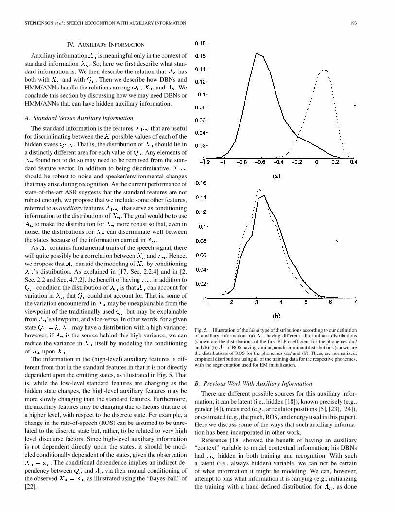
The information in the (high-level) auxiliary features is dif-ferent from that in the standard features in that it is not directlydependent upon the emitting states, as illustrated in Fig. 5. Thatis, while the low-level standard features are changing as thehidden state changes, the high-level auxiliary features may bemore slowly changing than the standard features. Furthermore,the auxiliary features may be changing due to factors that are ofa higher level, with respect to the discrete state. For example, achange in the rate-of-speech (ROS) can be assumed to be unre-lated to the discrete state but, rather, to be related to very highlevel discourse factors. Since high-level auxiliary informationis not dependent directly upon the states, it should be mod-eled conditionally dependent of the states, given the observation

. The conditional dependence implies an indirect de-pendency between and via their mutual conditioning ofthe observed , as illustrated using the “Bayes-ball” of[22].

Fig. 5. Illustration of the ideal type of distributions according to our definitionof auxiliary information: (a) X having different, discriminant distributions(shown are the distributions of the first PLP coefficient for the phonemes /ao/and /f/); (b)A of ROS having similar, nondiscriminant distributions (shown arethe distributions of ROS for the phonemes /ao/ and /f/). These are normalized,empirical distributions using all of the training data for the respective phonemes,with the segmentation used for EM initialization.

B. Previous Work With Auxiliary Information

There are different possible sources for this auxiliary infor-mation; it can be latent (i.e., hidden [18]), known precisely (e.g.,gender [4]), measured (e.g., articulator positions [5], [23], [24]),or estimated (e.g., the pitch, ROS, and energy used in this paper).Here we discuss some of the ways that such auxiliary informa-tion has been incorporated in other work.

Reference [18] showed the benefit of having an auxiliary“context” variable to model contextual information; his DBNshad hidden in both training and recognition. With sucha latent (i.e., always hidden) variable, we can not be certainof what information it might be modeling. We can, however,attempt to bias what information it is carrying (e.g., initializingthe training with a hand-defined distribution for , as done


in [18]). Zweig discussed, but never experimented with, usingreal and continuous data (e.g., articulator positions) for ; wecontinue his line of research in using auxiliary variables withreal data in our experiments.

Discrete auxiliary information with real data has previouslybeen investigated using the gender (male/female) of the speaker[4] or the ROS (slow/average/fast) of the utterance [25]. A sep-arate acoustic model is used for each of the discrete values of

so as to have distributions that are more adapted for the re-spective types of speech. While the is known with certaintyin training the models (at least in the case of using gender), aclassifier is used in recognition to infer its value. In this paper wecontinue this work in the context of certain of our HMM/ANNsystems (those that use discretized auxiliary information) by ex-amining the effect of auxiliary information that is extracted di-rectly from the speech signal (pitch, energy and ROS) instead ofby hand-labeling (e.g., gender) or by a forced alignment (e.g.,ROS of [25]).

A continuous auxiliary variable with data in both training andtesting was used in [15], where auxiliary information related topitch and energy characteristics was used. They showed howusing in a standard manner in speaker-dependent phonemeor isolated word recognition typically increases the error rate.However, if conditions the distributions of in conditionalGaussians, then the error rate decreases. This fits in with ourargument that certain auxiliary information needs to condition

’s distribution as well as possibly be independent of , bothof which were done successfully in [15]. In this paper, we alsoinvestigate having conditional pitch and energy related features(as well as ROS). We further this work by looking at the effectof hiding the continuous auxiliary feature during recognition, bylooking at the effect of having this auxiliary feature itself mod-eled dependent upon the state, and by using mixture models.Additionally, we are looking at the broader task of speaker-in-dependent, spontaneous speech recognition in noisy conditions.

While a discretized ROS was used in [25] above, a continuousROS was used in [26] to condition the transition probabilitiesout of the discrete states. In this paper we show how the emissiondistribution of can also be conditioned by a continuous ROS(like [25] but using a continuous ROS instead).

C. Auxiliary Information Modeling

1) DBNs: The various methods outlined below for includingin GMM based modeling can also be done in the framework

of HMMs. However, different software would need to be de-veloped for handling each change in the assumptions for han-dling . DBNs provide the general framework for being ableto handle any of these assumptions in the same software [18].

a) Only [Baseline, Fig. 2(a)]: Equivalent to standardHMMs, the “BASELINE” system models the emission distri-bution using GMMs with mixture components as

(6)

The elements of are assumed to be conditionally indepen-dent of each other, given the state and mixture component,

meaning that the mixture components have zeros off of thediagonal of each covariance matrix. Doing so reduces thecomplexity in the models and allows more robust models to belearned without the need for large amounts of data that verycomplex models would demand for effective learning.

b) [Fig. 2(b)]: Equivalent to ap-pending to and using the single feature vector in a stan-dard HMM, the “ ” system models theemission distribution with GMMs as

(7)

(8)

As in the BASELINE system, all covariance matrices have zerosoff of the diagonal. Since is dependent upon but condi-tionally independent of (given and ), it is not, ac-cording to our definition, truly auxiliary.

c) , [No Assumptions, Fig. 2(c)]: The ,system enhances the “ ” by conditioningthe elements of the mixture models for upon the respectiveelements of the mixture models for . This gives conditionalGaussians in the mixture components for and regular Gaus-sians in the mixture components for , lettingbe modeled as

(9)

(10)

Thus, is serving as a mid-level auxiliary variable to . Byhaving condition the distribution for , some of the covari-ance between the elements is further modeled implicitly; that is,both and allow more modeling of ’s covariance foreach state. The conditional GMMs in Fig. 3 each illustrate howcovariance is modeled with a mixture variable (i.e., the plots arenot spherical); they also illustrate how the covariance is furthermodeled with an auxiliary variable (i.e., in comparing the twographs, each mixture component shifts according to its respec-tive weight and to the value (low versus high) of the auxiliaryvariable). Note that the use of (10) instead of (8) represents asmall increase in the computation for each mixture. That is, as(10) uses conditional GMMs, there is an additional multiplica-tion and addition to shift each mean of according to the valueof (assuming ’s value is available).

d) [Fig. 2(d)]: Equation (10) in-cludes in the state-dependent mixture model. However, ourstandard way of incorporating involves treating as inde-pendent of . As and have a common child , theyare actually dependent upon each other if that common child isobserved [22]. As this observation is always present inour work, we specify that the independence between andmust be conditioned upon this observation; hence, we specify

in the conditional part of “ .”


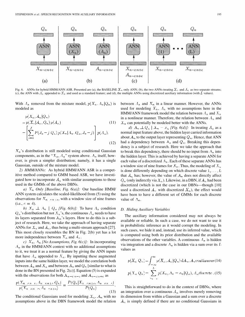
Fig. 6. ANNs for hybrid HMM/ANN ASR. Presented are (a), the BASELINE X only ANN; (b), the two ANNs treatingX and A as two separate streams;(c), the ANN with A appended toX and used as a standard feature; and (d), the multiple ANNs using discretized auxiliary information (with L values).

With removed from the mixture model, ismodeled as

(11)

(12)

’s distribution is still modeled using conditional Gaussiancomponents, as in the “ ” system above. itself, how-ever, is given a simpler distribution; namely, it has a singleGaussian, outside of the mixture model.

2) HMM/ANNs: As hybrid HMM/ANN ASR is a compet-itive method compared to GMM based ASR, we have investi-gated how to incorporate with similar assumptions to thoseused in the GMMs of the above DBNs.

a) Only [Baseline, Fig. 6(a)]: Our baseline HMM/ANN system calculates the scaled-likelihood from (5) using theobservations for , with a window size of nine frames(i.e., ).

b) [Fig. 6(b)]: To have condition’s distribution but not ’s, the continuous needs to have

its layers separated from ’s layers. How to do this is a sub-ject of research. Here, we take the approach of having separateANNs for and , thus being a multi-stream approach [27].This most closely resembles the BN in Fig. 2(b) yet has a lotmore independence between and .

c) , [No Assumptions, Fig. 6(c)]: In incorporatingin the HMM/ANN context with no additional assumptions

to it, we treat it as a normal feature by giving the ANN inputsthat have appended to . By inputting these augmentedinputs into the same hidden layer, we model the correlation bothbetween and and between and [similar to what isdone in the BN presented in Fig. 2(c)]. Equation (5) is expandedwith the observations for both and as

(13)The conditional Gaussians used for modeling , with noassumptions above in the DBN framework model the relation

between and in a linear manner. However, the ANNsused for modeling , with no assumptions here in theHMM/ANN framework model the relation between andin a nonlinear manner. Therefore, the relation between and

can potentially be modeled better with the ANNs.d) [Fig. 6(d)]: In treating as a

normal input feature above, the hidden layer carried informationabout to the output layer representing . Hence, that ANNhad a dependency between and . Breaking this depen-dency is a subject of research. Here we take the approach thatto break this dependency, there should be no input from intothe hidden layer. This is achieved by having a separate ANN foreach value of a discretized . Each of these separate ANNs hasa window size of nine frames for . Thus, the modeling ofis done differently depending on which discrete valuethat has; however, the value of does not directly affect

(only indirectly via ). Likewise, in a DBN, if had beendiscretized (which is not the case in our DBNs—though [10]used a discretized with discretized ), the effect wouldhave been to have a different set of GMMs for each discretevalue of .

D. Hiding Auxiliary Variables

The auxiliary information considered may not always beavailable or reliable. In such a case, we do not want to use itin probabilistic inference as it would corrupt the modeling. Insuch cases, we hide it and, instead, use its inferred value, whichis computed using both its prior distribution and the availableobservations of the other variables. A continuous is hiddenvia integration and a discrete is hidden via a sum over itsvalues as

(14)

(15)

This is straightforward to do in the context of DBNs, wherean integration over a continuous involves merely removingits dimension from within a Gaussian and a sum over a discrete

is simply defined if there are no conditional Gaussians in


the distribution. This is similar to the work done in missing fea-ture theory [28], where certain elements of are integratedout when they are suspected of being corrupted by noise. Notethat if has conditional Gaussians dependent upon a hidden,continuous , there would be additional computation involved(all simple multiplications, divisions, and additions). This is dueto the fact that all the elements are correlated with each other viathis hidden, continuous .

Regarding the case with ANNs, a discrete can easily behidden; as there is an ANN for each value of , we do aweighted sum of the posteriors from each ANN (the weights

are the distribution of in the training data). A con-tinuous can not easily be hidden, as it serves as an input intoan ANN. Hence, for our HMM/ANN systems, we only presentsystems with hidden for the cases where is discrete (i.e.,the HMM/ANN systems).

V. EXPERIMENTS

We have done our experiments using the OGI Numbers data[29], which contains free format numbers spoken over the tele-phone. As done in other work [30], we used 3233 utterances,covering 92 min, from the database for training; this is a subsetof the training list suggested by the database. We used a subsetof 1206 utterances of the suggested development set for evalu-ating the performance of the systems. As done in other workwith the OGI Numbers database at IDIAP, there were thirtywords (including silence) in the lexicon, composed of 27 mono-phone models (the three stops in the lexicon, /t/, /d/, and /k/were each represented as two monophones: one for the closureand one for the release of each respective stop). In the case ofthe DBNs, the silence and closure models were each modeledwith one state models, the releases were modeled with two statemodels, and all of the other monophones were modeled withthree state models, as done in related work at IDIAP. In the caseof the HMM/ANNs, the minimum state duration for trainingeach monophone is the same as the number of states used forthe respective monophone model in the DBNs, as the trainingof both types of systems is based on the same (initial) segmen-tation of OGI Numbers used in-house at IDIAP (this segmenta-tion, in the case of the DBNs is only used to determine the initialparameters to be used in EM training); the minimum state dura-tion for each monophone of the HMM/ANNs in recognition isthree frames, reflecting the constraint of the decoder used that allstates have the same minimum state duration. With the DBNs,except if noted, 12 mixture components were used in the (con-ditional) GMMs; this number of components was chosen so asto provide reasonable recognition results while not being toocomputationally complex. For all features we used a frame rateof 12.5 ms. The standard features used are 13 perceptual linearprediction (PLP) coefficients in addition to their approximatefirst and second derivatives, giving a total feature vector of 39elements (as the HMM/ANNs have inputs spanning nine timeframes, they have 351 inputs related to the PLP coefficients, notcounting any auxiliary feature inputs); the evaluation windowsize was 25 ms. Some of these results have appeared in [31].All significance tests are done on the word error rate (WER)with 99% confidence with a standard proportion test, assuminga binomial distribution for the targets and using a normal ap-

TABLE IEVALUATION OF PITCH ESTIMATION ALGORITHM FOR 5 MALE AND 5 FEMALE

UTTERANCES. Gross Error = n =n , WHERE n IS THE TOTAL NUMBER OF

COMPARISONS FOR WHICH THE DIFFERENCE (ABSOLUTE VALUE) BETWEEN

THE ESTIMATED PITCH AND THE REFERENCE PITCH IS GREATER THAN 20% OF

THE REFERENCE PITCH AND n IS THE TOTAL NUMBER OF COMPARISONS FOR

WHICH BOTH THE ESTIMATED PITCH FREQUENCY AND THE REFERENCE PITCH

REPRESENT VOICED SPEECH. HIGH GROSS ERROR AND LOW GROSS ERROR

BASICALLY REPRESENT THE PITCH DOUBLING EFFECT AND PITCH HALVING

EFFECT, RESPECTIVELY. AMD—ABSOLUTE MEAN DEVIATION

proximation. Recognition with the DBNs is done using a modi-fication of the inference algorithm that finds the most likely paththrough the states (i.e., Viterbi decoding); recognition withthe HMM/ANNs is done with Viterbi decoding.

A. Auxiliary Information Examined

We are looking at three types of auxiliary information:rate-of-speech (ROS), pitch (i.e., the fundamental frequency

), and short-term energy (in the logarithm domain). They areall fundamental features of speech that are speaker-dependentbut which can also change within a given speaker according toprosodic conditions and the environment. The auxiliary infor-mation (estimated from the clean speech signal) is always usedin training all of the systems (except in training the BASELINEsystems, which never use auxiliary information). In recogni-tion, their values are estimated from the speech signal under thesame clean or noisy conditions that the standard features arecalculated from. If the estimated auxiliary information valuesare used in the recognition tests, the auxiliary information isconsidered observed; otherwise, it is considered hidden. Aswith the standard features, all auxiliary features are estimatedusing a frame rate of 12.5 ms.

1) Pitch: The absence or presence of pitch is highly corre-lated with the phonemes. Hence, there is some relation betweenthe states and this auxiliary feature; however, this relation is be-tween groups of states (voiced versus unvoiced) and the auxil-iary feature. Also, it has been observed in the literature (e.g.,[32]) that pitch affects the estimation of the spectral envelope,in particular, the estimation of the spectral peaks, making thestandard features sensitive to changes in pitch. Thus, we mayexpect a certain correlation between the standard features andpitch. The auxiliary feature of pitch was estimated using thesimple inverse filter tracking (SIFT) algorithm [33], also witha window size of 25 ms (note that we did not take its logarithm,as could be done [15]). A five-point median smoothing was per-formed on the estimated pitch contour. We evaluated our pitchestimator with speech from five males and five females (witha total duration of approximately five minutes) from the Keelepitch database [34]. The results of this evaluation in Table I showthat the pitch estimation is reliable.


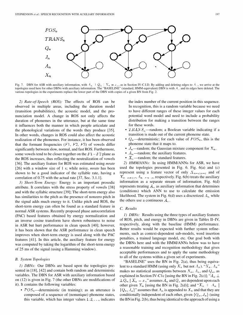
Fig. 7. DBN for ASR with auxiliary information, with A ??Q j X = x , as in Section IV-C.I.D. By adding and deleting edges to A , we arrive at thetopologies used here for other DBNs with auxiliary information. The “BASELINE” (standard, HMM-equivalent) DBN is with A and its edges here deleted. Thevarious topologies in the experiments replace the lower part of the DBN with copies of a given BN from Fig. 2.

2) Rate-of-Speech (ROS): The effects of ROS can beobserved in multiple areas, including the duration model(transition probabilities), the acoustic model, and the pro-nunciation model. A change in ROS not only affects theduration of phonemes in the utterance, but at the same timeit influences both the manner in which people articulate andthe phonological variations of the words they produce [35].In other words, changes in ROS could also affect the acousticrealization of the phonemes. For instance, it has been observedthat the formant frequencies ( , , ) of vowels differsignificantly between slow, normal, and fast ROS. Furthermore,some vowels tend to be closer together on the – plane asthe ROS increases, thus reflecting the neutralization of vowels[36]. The auxiliary feature for ROS was estimated using mrate[26] with a window size of 1 s; while noisy, mrate has beenshown to be a good indicator of the syllable rate, having acorrelation of 0.75 with the actual rate [37, Sec. 3.1.1].

3) Short-Term Energy: Energy is an important prosodicattribute. It correlates with the stress property of vowels [38]and with the syllabic structure [39]; The short-term energy alsohas similarities to the pitch as the presence of nonzero pitch inthe signal adds much energy to it. Unlike pitch and ROS, theshort-term energy can often be found as a standard feature innormal ASR systems. Recently proposed phase autocorrelation(PAC) based features obtained by energy normalization andan inverse cosine transform have shown robustness to noisein ASR but hurt performance in clean speech [40]; however,it has been shown that the ASR performance in clean speechimproves when short-term energy is used along with the PACfeatures [41]. In this article, the auxiliary feature for energywas computed by taking the logarithm of the short-term energyof 25 ms of the signal (using a Hamming window).

B. System Topologies

1) DBNs: Our DBNs are based upon the topologies pre-sented in [18], [42] and contain both random and deterministicvariables. The DBN for ASR with auxiliary information basedon (12) is given in Fig. 7 (the other DBNs are modifications ofit). It contains the following variables:

• —deterministic (in training); as an utterance iscomposed of a sequence of (nonunique) phoneme states,this variable, which has integer values , indicates

the index number of the current position in this sequence.In recognition, this is a random variable because we needto have different ranges of these integer values for eachpotential word model and need to include a probabilitydistribution for making a transition between the rangesfor these words.

• —random; a Boolean variable indicating if atransition is made out of the current phoneme state.

• —deterministic; for each value of , this is thephoneme state that it maps to.

• —random; the Gaussian mixture component for .• —random; the auxiliary features.• —random; the standard features.

2) HMM/ANNs: In using HMM/ANNs for ASR, we haveused the topologies presented in Fig. 6. Fig. 6(a) and (c)represent using a feature vector of only and of

, respectively. Fig. 6(b) treats the auxiliaryinformation as a separate stream of information. Fig. 6(d)represents treating as auxiliary information that determines(conditions) which ANN to use to calculate the emissionlikelihood. The system in Fig. 6(d) uses a discretized whilethe others use a continuous .

C. Results

1) DBNs: Results using the three types of auxiliary featuresof ROS, pitch, and energy in DBNs are given in Tables II–IV,respectively, along with the baseline (HMM) performance.Better results would be expected with further system refine-ments, such as context-dependent sub-models, word insertionpenalties, a trained language model, etc. Our goal both withthe DBNs here and with the HMM/ANNs below was to havea reasonable training and recognition methodology that givesacceptable performances and to apply the same methodologyto all of the systems within a given set of experiments.

“BASELINE” uses the BN in Fig. 2(a), thus being equiva-lent to a standard HMM (using only but not ). “ ”makes no statistical assumptions between , , and , asexplained in Section IV-C1c [using the BN in Fig. 2(c)]; “

” assumes and are dependent upon eachother given [using the BN in Fig. 2(d)]; and “

” assumes that is appended to and that they areconditionally independent of each other, given (usingthe BN in Fig. 2(b), thus being identical to the approach of using a


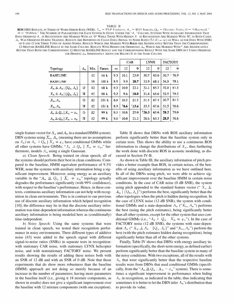
TABLE IIROS DBN RESULTS, IN TERMS OF WORD-ERROR-RATE (WER). X = PLP Features, A = ROS feature, Q = Discrete State, O = \Observed; "H = \Hidden:" THE NUMBER OF PARAMETERS FOR EACH SYSTEM IS GIVEN. UNDER THE ‘A ’ COLUMN, SYSTEMS WITH AUXILIARY INFORMATION THAT

HAVE OBSERVED A IN RECOGNITION ARE MARKED WITH AN ‘O’ WHILE THOSE WITH HIDDEN A IN RECOGNITION ARE MARKED WITH ‘H’; IN BOTH CASES,A WAS OBSERVED DURING TRAINING. RESULTS ARE REPORTED ON CLEAN DATA (SIGNAL TO NOISE RATIO (SNR) =1) AS WELL AS FOR DATA WITH SNRS

OF 0 AND 12 FOR THREE TYPES OF ADDED NOISES. RESULTS WHICH ARE MARKED WITH BOLD ARE SIGNIFICANTLY BETTER THAN THE CORRESPONDING

12-MIXTURE BASELINE RESULT IN THE SAME COLUMN. RESULTS WITH HIDDEN (OR OBSERVED) A WHICH ARE MARKED WITH ARE SIGNIFICANTLY

BETTER THAN BOTH THE CORRESPONDING 12-MIXTURE BASELINE RESULT AND THE CORRESPONDING RESULT WITH THE SAME DBN BUT USING OBSERVED

(OR HIDDEN) A IMMEDIATELY ABOVE (OR BELOW) IT IN THE SAME COLUMN

single feature vector for and in a standard HMM system).DBN systems using , (meaning there are no assumptionson ) or have conditional GMMs whileall other systems have GMMs; “ ,” fur-thermore, models using a single Gaussian.

a) Clean Speech: Being trained on clean speech, all ofthe systems should perform their best in clean conditions. Com-pared to the baseline, HMM equivalent performance of 9.3%WER, none the systems with auxiliary information bring a sig-nificant improvement. Moreover, using energy as an auxiliaryvariable in the “ ” topology actuallydegrades the performance significantly (with 99% confidence),with respect to the baseline’s performance. Hence, in these con-texts, continuous auxiliary information can not help with recog-nition in clean environments. This is in contrast to our previoususe of discrete auxiliary information which helped recognition[10]; the difference may lie in that the discrete auxiliary infor-mation was time-dependent information whereas the continuousauxiliary information is being modeled here as (conditionally)time-independent.

b) Noisy Speech: Using the same systems that weretrained in clean speech, we tested their recognition perfor-mance in noisy environments. Three different types of additivenoise [43] were added to the speech signal with differentsignal-to-noise ratios (SNRs) in separate tests in recognition:with stationary CAR noise, with stationary LYNX helicopternoise, and with nonstationary FACTORY noise. We presentresults showing the results of adding these noises both withan SNR of 12 dB and with an SNR of 0 dB. Note that thoseexperiments that do show more robustness than the baseline(HMM) approach are not doing so merely because of anincrease in the number of parameters; having more parametersin the baseline itself (i.e., giving it 18 mixture components, asshown in results) does not give a significant improvement overthe baseline with 12 mixture components (with one exception).

Table II shows that DBNs with ROS auxiliary informationperform significantly better than the baseline system only incertain tests. This shows the ability to use a continuous ROSinformation to change the distributions of , thus furtheringthe work done with discrete ROS in acoustic modeling, as dis-cussed in Section IV-B.

As shown in Table III, the auxiliary information of pitch pro-vides a better example than ROS, in certain noises, of the ben-efits of using auxiliary information as we have outlined here.In all of the DBNs using pitch, we were able to achieve sig-nificant improvement over the baseline HMM in certain noiseconditions. In the case of CAR noise (0 dB SNR), the systemusing pitch appended to the standard feature vector (“

”) performs the best, significantly better than theother topologies when the pitch is hidden during recognition. Inthe case of LYNX noise (12 dB SNR), the system with condi-tional GMMs and a state-dependent (“ ”) performsthe best (using the pitch estimates), being significantly betterthan all other systems, except for the other system that uses con-ditional GMMs (i.e., “ ”). In the case ofFACTORY noise (12 dB SNR), the systems with state-depen-dent (“ ” and “ ”) perform thebest (with the pitch estimates hidden during recognition), beingsignificantly better than all of the other systems.

Finally, Table IV shows that DBNs with energy auxiliary in-formation (specifically, the short-term energy, as defined earlier)perform significantly better than the baseline system in many ofthe noisy conditions. With two exceptions, all of the results with

that were significantly better than the respective baselineresults were from DBNs that used conditional GMMs (specifi-cally, from the “ ” system). There is some-times a significant improvement in performance when hiding

in recognition, as indicated in the table, thus indicating thatsometimes it is better to let the DBN infer ’s distribution thanto provide its value.


TABLE IIIPITCH DBN RESULTS, WITH A SIMILAR SETUP TO THAT OF TABLE II EXCEPT THAT A = Pitch

TABLE IVENERGY DBN RESULTS, WITH A SIMILAR SETUP TO THAT OF TABLE II EXCEPT THAT A = Energy

TABLE VROS ANN RESULTS, IN TERMS OF WORD-ERROR-RATE (WER). X = PLP Features, A = ROS Feature, Q = Discrete State, O = \Observed",H = \Hidden:"; THE NUMBER OF PARAMETERS FOR EACH SYSTEM IS GIVEN (IN THE CASE OF “A ??Q j X = x ,” WHICH HAS MULTIPLE ANNS, THIS

IS THE SUM OF THE PARAMETERS IN ALL OF ITS ANNS). UNDER THE ‘A ’ COLUMN, SYSTEMS WITH AUXILIARY INFORMATION THAT HAVE OBSERVED A IN

RECOGNITION ARE MARKED WITH AN ‘O’ WHILE THOSE WITH HIDDEN A IN RECOGNITION ARE MARKED WITH ‘H’; IN BOTH CASES, A WAS OBSERVED

DURING TRAINING. HIDDEN AUXILIARY INFORMATION IS ONLY USED IN THE SYSTEM WITH A ??Q j X = x (WHICH HAS THREE DISCRETE VALUES FOR

A ) FOR THEORETICAL REASONS. RESULTS ARE REPORTED ON CLEAN DATA (SNR =1) AS WELL AS FOR DATA WITH SNRS OF 0 AND 12 FOR THREE TYPES

OF ADDED NOISES. RESULTS WHICH ARE MARKED WITH BOLD ARE SIGNIFICANTLY BETTER THAN THE CORRESPONDING BASELINE RESULT IN THE SAME

COLUMN. RESULTS WITH HIDDEN (OR OBSERVED) A WHICH ARE MARKED WITH ARE SIGNIFICANTLY BETTER THAN BOTH THE CORRESPONDING BASELINE

RESULT AND THE CORRESPONDING RESULT WITH THE SAME ANNS BUT USING OBSERVED (OR HIDDEN) A IMMEDIATELY ABOVE (OR BELOW) IT IN THE SAME

COLUMN (THIS DOES NOT OCCUR IN THIS TABLE BUT DOES OCCUR IN THE RELATED TABLES VI AND VII)

2) HMM/ANNs: Results using HMM/ANNs and the auxil-iary features are given in Tables V–VII, along with the base-line results. The various systems used for HMM/ANN hybrids

(note that no DBNs were involved with the ANNs) were pre-sented in Fig. 6. The baseline system uses only the standard fea-tures as its inputs, using (5) to estimate the scaled-likelihoods.


TABLE VIPITCH ANN RESULTS, WITH A SIMILAR SETUP TO THAT OF EXCEPT THAT A = Pitch

TABLE VIIENERGY ANN RESULTS, WITH A SIMILAR SETUP TO THAT OF EXCEPT THAT A = Energy

systems use separate ANNs for and forto jointly estimate the scaled-likelihoods. The , sys-

tems uses both the standard and auxiliary features as its inputs ina standard ANN, using (13) to estimate the scaled-likelihoods.Finally, the systems use multiple ANNs,one for each discrete value of to estimate the scaled-likeli-hoods and with each one using only the standard features as itsinputs.

During the training phase, it is only the ANNs which aretrained (using back propagation with cross-validation over avalidation set of 357 utterances from speakers not occurringin either the training or testing of the ANNs), which is doneusing the previously supplied segmentation. The HMMs are nottrained themselves (their emission distributions are handled bythe ANNs and their transition probabilities are set to a uniformdistribution); their role is to take the scaled-likelihoods for doingViterbi decoding.

a) Clean Speech: As with the DBNs, all of the HMM/ANN systems were trained on clean speech and have their bestperformance when presented with clean speech. With referenceto the baseline HMM/ANN, which uses only standard features,only one of the systems with observed auxiliary informationpresented in the tables performs better. Hiding the (discrete)auxiliary information, as explained in Section IV-D, did notimprove the recognition performance. The one HMM/ANNsystem with auxiliary information that did well used energy asa (discrete) conditioning variable, thus showing the potentialfor using ANNs tailored to different values of a discrete .

b) Noisy Speech: Using auxiliary information in HMM/ANNs in noisy speech brings mixed results. None of the sys-

Fig. 8. For selected states ofQ , plots of the correlation between PLP [1] andan A representing energy. These are taken from the distributions for PLP [1]in the “A ;X ” system from Table IV. Only the first states of each phonemeare represented here.

tems with auxiliary information performs significantly betterthan the baseline in FACTORY noise. Using pitch as auxiliaryinformation was of some benefit, but only under LYNX noiseconditions. As with the DBNs, the best auxiliary informationof the three tested in spontaneous, noisy speech was energy. Ofthe various systems tested with energy, the , system typ-ically did well in noise, at least in CAR and LYNX noise, whereit performed significantly better than the baseline system.


Fig. 9. Calculated versus inferred pitch. For a given utterance from the testingset, the calculated (observed) pitch (using SIFT) in clean conditions is given in(a). Using the “X ;A ” system from Table III, the inferred pitch in 12 dB SNRFACTORY noise is given in (b); the actual inferred values are in the dashedline while the smoothed version of the dashed line is given in a solid line.The distance between the (unsmoothed) inferred pitch values and the observedpitch (in clean conditions) shown here is typical for the testing set in this noisecondition. In this given noisy condition, the DBN did significantly better overthe whole test set with such inferred values instead of the calculated (observed)values.

D. Behavior of Auxiliary Information in Trained Systems

When the distribution of in the DBNs is conditioned by, there will be different amounts of correlation between

and for each value of the state . That is, the emission dis-tributions of for certain hidden states are more dependentupon the value of than others. Fig. 8 illustrates how, for cer-tain phoneme states, there is a stronger correlation than othersbetween and the auxiliary variable of energy. A stronger cor-relation between and for a given state will be reflectedin a larger absolute value of the regression weights for thatstate. Even if and are not directly connected, the distri-

Fig. 10. Inferring energy using a sample utterance, using the “A ?? Q jX = x ” system from Table IV. The thick and thin solid plots show thecalculated energy in noisy and clean speech, respectively. The dashed plot showsthe inferred energy (with median smoothing). The noisy speech is in 0 dB SNRFACTORY noise. The distances between the inferred values (before smoothing)and both the calculated energy in a clean environment and the calculated energyin this noisy environment are both representative in testing in this noise.

bution of will have a unique weight upon for each valueof (since is dependent upon ).

When a conditioning is hidden in the DBNs, its inferreddistribution is used during recognition. This is based on itsprior distribution learned in training as well as the observationsand prior distributions for the other variables in the DBN.As shown in the experimental studies, using this inferreddistribution sometimes gives better results in recognition thanusing the actual calculated values. Fig. 9 illustrates the inferredvalue of pitch during noise versus its calculated value in cleanconditions. The inferred values do vary a lot over the actualestimated values, in comparing the dashed line in Fig. 9(b) withthe line in Fig. 9(a). However, when the inferred values aremedian smoothed (using a window of five values and with allpitch values under 80 Hz being set to zero), the pitch contouris similar to the actual estimates in clean speech. Fig. 10gives an alternate view of what can happen when inferringthe values of an auxiliary variable, in this case, that of energy.The recognition experiments that the illustrated utterance wastaken from did better with hidden energy than with observedenergy; however, the inferred energy values are closer to thenoisy values than to the underlying, clean speech values.Nevertheless, it was better in this set of experiments to use theinferred values.

VI. CONCLUSION

Auxiliary information makes acoustic modeling in ASR morerobust to noise in many cases with DBNs and, to a lesser extent,with HMM/ANNs as well. Improvements with the HMM/ANNscould be possible if there could be a way for to serve as apurely conditioning variable to without having to discretizeit and make a separate ANN for each discrete value; with thetraining data being divided among many ANNs, each individual


ANN will not be as robustly trained with the reduced amount oftraining data. Hence, future work would involve having a singleANN whose parameters dynamically adapt to the value of ,just as the conditional Gaussians do.

In DBNs with auxiliary information, it is important to useto “shift” conditional GMMs that model as opposed to

having GMMs that do not take into account; for a smallamount of additional computation, this allows us to directlymodel the correlation between and and to indirectlymodel even more of the correlation within . This was bestillustrated in the case of using energy, where in noisy speech ofeither LYNX or FACTORY noise at an SNR of 12 dB, a rela-tive reduction of almost 50% in the WER was observed with the

topology.Using pitch as an auxiliary variable in the conditional Gaus-

sians of DBNs did prove useful, showing there is correlation be-tween pitch and . However, we see that using it as a standardfeature (appended to the feature vector), as represented by thetopology “ ” is sometimes significantlybetter than using it with conditional GMMs. Nevertheless, incertain noises (i.e., LYNX), using the conditional GMMs provedbetter. The pitch, as opposed to the energy, may have had moreeffect in the use of appending it as a standard feature because thepresence of pitch indicates whether there is a voiced phoneme ornot; however, energy may be harder to use to give a reliable dis-crimination between phonemes. Hence, the proper use of pitchdeserves more study in future work. Overall, ROS did not pro-vide as significant gains as using the energy and pitch; futurework with ROS would involve having smoother estimates of itas well as using it on a larger database containing more varia-tions in the speaking rate.

Hiding the in the conditional GMMs sometimes makesthe DBNs even more robust to noise. By using the inferredvalues for , we can sometimes achieve a significant perfor-mance improvement over when we use the actual observationsfor . This was best illustrated with the performances in 12 dBSNR FACTORY noise of the various DBNs with pitch auxiliaryinformation, where the tests with the pitch hidden were signifi-cantly better than respective tests with the estimated (observed)pitch values; the WER was reduced by a relative 19%–39%.

The most interesting line of future work would be to investi-gate the use of having the auxiliary variable be time-depen-dent, such that its distribution is modeled as . Thebenefit of this is that, when inferring the distribution of a hidden

, its posterior distribution is constrained by the inferred valueof the hidden ; this better models the evolution of , es-pecially if using an whose values change slowly over time.However, in using a time-dependent, continuous-valued, hidden

, exact probabilistic inference (such as that used in our work)is intractable [20], in which case approximate inference algo-rithms need to be explored [13], [44, Chapter 5].

ACKNOWLEDGMENT

This work benefited from earlier research done by J. CarmonaEscofet as well as from input from I. Lapidot, I. McCowan,and D. Gatica-Perez as well as from the examiners of the firstauthor’s thesis. M. Shajith Ikbal provided the decoder for theHMM/ANN experiments. The comments of the anonymous re-viewers helped to greatly improve the quality of this paper.

REFERENCES

[1] L. R. Rabiner, “A tutorial on hidden Markov models and selected appli-cations in speech recognition,” Proc. IEEE, vol. 77, pp. 257–286, Feb.1989.

[2] J. A. Bilmes, “Natural Statistical Models for Automatic Speech Recog-nition,” Ph.D. dissertation, Univ. California, Berkeley, 1999.

[3] C. J. Wellekens, “Explicit time correlation in hidden Markov models forspeech recognition,” in Proc. 1987 IEEE Int. Conf. Acoustics, Speech,and Signal Processing (ICASSP-87), vol. 1, Dallas, TX, Apr. 1987, pp.384–386.

[4] Y. Konig and N. Morgan, “GDNN: A gender-dependent neural networkfor continuous speech recognition,” in Proc. 1992 Int. Joint Conf. NeuralNetworks (IJCNN), Baltimore, MD, June 1992, pp. 332–337.

[5] T. A. Stephenson, H. Bourlard, S. Bengio, and A. C. Morris, “Automaticspeech recognition using dynamic Bayesian networks with both acousticand articulatory variables,” in Proc. 6th Int. Conf. Spoken Language Pro-cessing (ICSLP 2000), vol. 2, Beijing, China, Oct. 2000, pp. 951–954.

[6] R. G. Cowell, A. P. Dawid, S. L. Lauritzen, and D. J. Spiegelhalter, Prob-abilistic Networks and Expert Systems. New York: Springer-Verlag,1999.

[7] T. Dean and K. Kanazawa, “Probabilistic temporal reasoning,” in Proc.7th National Conf. Artificial Intelligence (AAAI-88), St. Paul, MN, 1988,pp. 524–528.

[8] S. L. Lauritzen, Graphical Models. Oxford, U.K.: Clarendon, 1996,vol. 17.

[9] H. Bourlard and N. Morgan, Connectionist Speech Recognition: A Hy-brid Approach. Boston, MA: Kluwer, 1993, vol. 247.

[10] T. A. Stephenson, M. Mathew, and H. Bourlard, “Modeling auxiliaryinformation in Bayesian network based ASR,” in Proc. 7th Eur. Conf.Speech Communication and Technology (EUROSPEECH ’01), vol. 4,Aalborg, Denmark, Sept. 2001, pp. 2765–2768.

[11] S. L. Lauritzen and F. Jensen, “Stable local computations with con-ditional Gaussian distributions,” Statist. Comput., vol. 11, no. 2, pp.191–203, Apr. 2001.

[12] F. V. Jensen, An Introduction to Bayesian Networks. London, U.K.:UCL, 1996.

[13] K. P. Murphy, “Dynamic Bayesian Networks: Representation, Inferenceand Learning,” Ph.D. dissertation, Univ. California, Berkeley, 2002.

[14] D. Koller, U. Lerner, and D. Angelov, “A general algorithm for approx-imate inference and its application to hybrid Bayes nets,” in Proc. 15thConf. Uncertainty in Artificial Intelligence (UAI–99), San Francisco,CA, July 1999, pp. 324–333.

[15] K. Fujinaga, M. Nakai, H. Shimodaira, and S. Sagayama, “Multiple-re-gression hidden Markov model,” in Proc. 2001 IEEE Int. Conf. Acous-tics, Speech, and Signal Processing (ICASSP-01), vol. 1, Salt Lake City,UT, May 2001, pp. 513–516.

[16] B. J. Frey, Graphical Models for Machine Learning and Digital Com-munication. Cambridge, MA: MIT Press, 1998.

[17] J. Pearl, Probabilistic Reasoning in Intelligent Systems: Networks ofPlausible Inference. New York: Morgan Kaufmann, 1988.

[18] G. G. Zweig, “Speech Recognition With Dynamic Bayesian Networks,”Ph.D. dissertation, Univ. California, Berkeley, 1998.

[19] L. E. Baum, “An equality and associated maximization technique in sta-tistical estimation for probabilistic functions of Markov processes,” In-equalities, vol. 3, pp. 1–8, 1972.

[20] U. Lerner and R. Parr, “Inference in hybrid networks: Theoretical limitsand practical algorithms,” in Proc. 17th Conf. Uncertainty in ArtificialIntelligence (UAI-2001), San Francisco, CA, Aug. 2001, pp. 310–318.

[21] X. Boyen and D. Koller, “Tractable inference for complex stochasticprocesses,” in Proc. 14th Conf. Uncertainty in Artificial Intelligence(UAI–98), San Francisco, CA, July 1998, pp. 33–42.

[22] R. D. Shachter, “Bayes-ball: The rational pastime (for determining ir-relevance and requisite information in belief networks and influencediagrams),” in Proc. 14th Conf. Uncertainty in Artificial Intelligence(UAI–98), San Francisco, CA, July 1998, pp. 480–487.

[23] J. R. Westbury, G. Turner, and J. Dembowski, X-ray Microbeam SpeechProduction Database User’s Handbook, 1st ed. Madison: Univ. Wis-consin, Waisman Center on Mental Retardation & Human Development,1994.

[24] A. Wrench, “Multichannel/multispeaker articulatory database for con-tinuous speech recognition research,” in PHONUS. Saarbrücken, Ger-many: Saarland Univ., Institute of Phonetics, 2000.

[25] F. Martínez, D. Tapias, and J.Álvarez, “Toward speech rate indepen-dence in large vocabulary continuous speech recognition,” in Proc. 1998IEEE Int. Conf. Acoustics, Speech, and Signal Processing (ICASSP-98),Seattle, WA, May 1998, pp. 725–728.


[26] N. Morgan, E. Fosler, and N. Mirghafori, “Speech recognition usingon-line estimation of speaking rate,” in Proc. 5th Eur. Conf. SpeechCommunication and Technology (EUROSPEECH ’97), vol. 4, Rhodes,Greece, September 1997, pp. 2079–2082.

[27] S. Dupont, “Etude et Développement D’architectures Multi-Bandes etMulti-Modales Pour la Reconnaissance Robuste de la Parole,” Ph.D. dis-sertation, Faculté Polytechnique de Mons, Mons, Belgium, 2000.

[28] A. C. Morris, M. P. Cooke, and P. D. Green, “Some solutions to themissing feature problem in data classification, with application to noiserobust ASR,” in Proc. 1998 IEEE Int. Conf. Acoustics, Speech, andSignal Processing (ICASSP-98), vol. 2, Seattle, WA, May 1998, pp.737–740.

[29] R. A. Cole, M. Fanty, M. Noel, and T. Lander, “Telephone speech Corpusdevelopment at CSLU,” in Proc. 3rd Int. Conf. Spoken Language Pro-cessing (ICSLP ’94), Yokohama, Japan, Sept. 1994.

[30] N. Mirghafori and N. Morgan, “Combining connectionist multi-bandand full-band probability streams for speech recognition of natural num-bers,” in Proc. 5th Int. Conf. Spoken Language Processing (ICSLP ’98),vol. 3, Sydney, Australia, November 1998, pp. 743–746.

[31] T. A. Stephenson, M. Magimai-Doss, and H. Bourlard, “Speechrecognition of spontaneous, noisy speech using auxiliary information inBayesian networks,” in Proc. 2003 IEEE Int. Conf. Acoustics, Speech,and Signal Processing (ICASSP-03), vol. 1, Hong Kong, April 2003,pp. 20–23.

[32] H. Hermansky, “Perceptual linear predictive (PLP) analysis of speech,”J. Acoust. Soc. Amer., vol. 87, no. 4, pp. 1738–1752, Apr. 1990.

[33] J. D. Markel, “The SIFT algorithm for fundamental frequency estima-tion,” IEEE Trans. Audio Electroacoust., vol. 20, no. 5, pp. 367–377,Dec. 1972.

[34] F. Plante, G. F. Meyer, and W. A. Ainsworth, “A pitch extractionreference database,” in Proc. 4th Eur. Conf. Speech Communicationand Technology (EUROSPEECH ’95), Madrid, Spain, Sept. 1995, pp.837–840.

[35] T. J. Hazen, “The Use of Speaker Correlation Information for AutomaticSpeech Recognition,” Ph.D. dissertation, Mass. Inst. Technol., 1998.

[36] H. Kuwabara, “Acoustic and perceptual properties of phonemes in con-tinuous speech as a function of speaking rate,” in 5th Eur. Conf. SpeechCommunication and Technology (EUROSPEECH ’97), vol. 2, Rhodes,Greece, September 1997, pp. 1003–1006.

[37] J. E. Fosler-Lussier, “Dynamic Pronunciation Models for AutomaticSpeech Recognition,” Ph.D., Univ. California, Berkeley, 1999.

[38] C. Wang and S. Seneff, “Lexical stress modeling for improved speechrecognition of spontaneous telephone speech in the JUPITER domain,”in Proc. 7th Eur. Conf. Speech Communication and Technology(EUROSPEECH ’01), vol. 4, Aalborg, Denmark, September 2001, pp.2761–2764.

[39] T. Nagarajan, H. A. Murthy, and R. M. Hegde, “Segmentation of speechinto syllable-like units,” in Proc. 8th Eur. Conf. Speech Communica-tion and Technology (EUROSPEECH ’03), vol. 4, Geneva, Switzerland,Sept. 2003, pp. 2893–2896.

[40] S. Ikbal, H. Misra, and H. Bourlard, “Phase autocorrelation (PAC) de-rived robust speech features,” in Proc. 2003 IEEE Int. Conf. Acoustics,Speech, and Signal Processing (ICASSP-03), vol. 2, Hong Kong, Apr.2003, pp. 133–136.

[41] S. Ikbal, H. Hermansky, and H. Bourlard, “Nonlinear spectral transfor-mations for robust speech recognition,” in Proc. 2003 IEEE Workshopon Automatic Speech Recognition and Understanding (ASRU ’03), St.Thomas, U.S. Virgin Islands, Nov. 2003, pp. 393–398.

[42] G. Zweig and M. Padmanabhan, “Dependency modeling with Bayesiannetworks in a voicemail transcription system,” in Proc. 6th Eur. Conf.Speech Communication and Technology (EUROSPEECH ’99), vol. 3,Budapest, Hungary, Sept. 1999, pp. 1135–1138.

[43] A. Varga, H. Steeneken, M. Tomlinson, and D. Jones, “The NOISEX-92Study on the Effect of Additive Noise on Automatic Speech Recogni-tion,” DRA Speech Research Unit, Malvern, U.K., 1992.

[44] H. Akashi and H. Kumamoto, “Random sampling approach to state es-timation in switching environments,” Automatica, vol. 13, pp. 429–434,July 1977.

[45] Proc. 7th European Conference on Speech Communication and Tech-nology (EUROSPEECH ’01), Aalborg, Denmark, Sept. 2001.

[46] Proc. 2003 IEEE International Conference on Acoustics, Speech, andSignal Processing (ICASSP-03), Hong Kong, Apr. 2003.

[47] Proc. 14th Conf. Uncertainty in Artificial Intelligence (UAI–98), SanFrancisco, CA, July 1998.

[48] Proc. 5th Eur. Conf. Speech Communication and Technology (EU-ROSPEECH ’97), Rhodes, Greece, Sept. 1997.

[49] Proc. 1998 IEEE Int. Conf. Acoustics, Speech, and Signal Processing(ICASSP-98), Seattle, WA, May 1998.

Todd A. Stephenson (S’01–M’04) received the B.S.degree in mathematics from the Pennsylvania StateUniversity in 1995; the M.Sc. degree in CognitiveScience and Natural Language from the Universityof Edinburgh, Edinburgh, U.K., in 1998; and thePh.D. degree from the Swiss Federal Institute ofTechnology at Lausanne (EPFL) in 2003.

From 1995 to 1997, he was with the ConsumerMarkets Division of AT&T Corp., Piscataway,NJ. From 1999 to 2003, he was with the SpeechProcessing Group of the Dalle Molle Institute for

Perceptual Artificial Intelligence (IDIAP) in Martigny, Switzerland. In thewinter of 2001, he was an Intern with the Information Sciences ResearchDivision of AT&T Labs-Research, Florham Park, NJ. His research interestsinclude automatic speech recognition, statistical pattern recognition, andcomputational linguistics.

Mathew Magimai Doss (S’03) received the B.E.degree in Instrumentation and Control Engineeringfrom the University of Madras, India, in 1996; theM.S. degree in computer science and engineeringfrom the Indian Institute of Technology, Madras,in 1999; and the PreDoctoral diploma from theSwiss Federal Institute of Technology at Lausanne(EPFL), Switzerland in 2000. Since August 2000,he has been pursuing the Ph.D. degree in the SpeechProcessing Group of the Dalle Molle Institutefor Perceptual Artificial Intelligence (IDIAP) in

Martigny, Switzerland.His research interests include speech processing, automatic speech and

speaker recognition, statistical pattern recognition, and artificial neuralnetworks.

Hervé Bourlard (M’89–SM’95–F’00) received theElectrical and Computer Science Engineering degreeand the Ph.D. degree in Applied Sciences both fromPolytechnic University of Mons, Belgium.

After having been a member of the ScientificStaff at the Philips Research Laboratory of Brussels(Belgium, 1982–1990) and an R&D Manager atL&H SpeechProducts (Belgium, 1990–1996), heis now Director of IDIAP (Dalle Molle Institutefor Perceptual Artificial Intelligence, Switzerland)and Professor at the Swiss Federal Institute of

Technology at Lausanne (EPFL). He is also Director of a National Center ofCompetence in Research in “Interactive Multimodal Information Manage-ment.” Having spent (since 1988) several long-term and short-term visits, asa Guest Scientist, at the International Computer Science Institute (ICSI) inBerkeley, CA, he is now an ICSI External Fellow and a member of the ICSIBoard of Trustees. His current interests mainly include signal processing,statistical pattern classification, multichannel processing, artificial neuralnetworks, and applied mathematics, with applications to speech processing,speech and speaker recognition, language modeling, computer vision, andmultimodal processing. He is the author/coauthor of two books and over 170reviewed papers and book chapters.

Dr. Bourlard has received a IEEE Paper Award. He is an IEEE Fellow “forcontributions in the fields of statistical speech recognition and neural networks.”He is a member of the program and/or scientific committees of numerous inter-national conferences and journal, is a past Editor-in-Chief of Speech Commu-nication, and a member of the IEEE Technical Committee on Neural NetworkSignal Processing. Over the last 15 years, he has initiated and managed nu-merous European projects.

IEEE TRANSACTIONS ON SPEECH AND AUDIO PROCESSING,...

Documents

Transcript of IEEE TRANSACTIONS ON SPEECH AND AUDIO PROCESSING,...