Dynamic Refraction StereoNigel J.W. Morris and Kiriakos N. Kutulakos, Member, IEEE

Abstract—In this paper we consider the problem of reconstructing the 3D position and surface normal of points on an unknown,

arbitrarily-shaped refractive surface. We show that two viewpoints are sufficient to solve this problem in the general case, even if the

refractive index is unknown. The key requirements are 1) knowledge of a function that maps each point on the two image planes to a

known 3D point that refracts to it, and 2) light is refracted only once. We apply this result to the problem of reconstructing the time-

varying surface of a liquid from patterns placed below it. To do this, we introduce a novel “stereo matching” criterion called refractive

disparity, appropriate for refractive scenes, and develop an optimization-based algorithm for individually reconstructing the position

and normal of each point projecting to a pixel in the input views. Results on reconstructing a variety of complex, deforming liquid

surfaces suggest that our technique can yield detailed reconstructions that capture the dynamic behavior of free-flowing liquids.

Index Terms—Stereo, time-varying imagery, shape-from-X, transparency, refractive index estimation.

Ç

1 INTRODUCTION

MODELING the time-varying surface of a liquid hasattracted the attention of many research fields, from

computer graphics [10], [14], [36], [39] and fluid mechanics[20] to oceanography [11], [28], [32], [58]. While great strideshave been achieved in the development of computersimulators that are physically accurate and visually correct[14], [36], capturing the time-varying behavior of a realliquid remains a challenging problem.

From the point of view of computer vision, analyzing thebehavior of liquids from videos poses several difficultiescompared to traditional 3D photography applications:

. No prior scene model. Spatiotemporal evolution isconstrained only by the laws of fluid mechanics,making it difficult to assume a low-degree-of-free-dom parametric model for such a scene [4], [57].

. Nonlinear light path. Liquid surfaces bend the incidentlight and, hence, a point below the surface will projectalong a nonlinear path to a viewpoint above it.

. Shape-dependent appearance modulation. Absorption,scattering, and Fresnel transmission cause the ap-pearance of points below the surface to depend on thelight’s path and, hence, on the surface shape [18].

. Turbulent behavior. Liquid flow is an inherentlyvolumetric phenomenon whose complete character-ization requires capturing both its time-varying sur-face and a vector field describing internal motion [59].

. Instantaneous 3D capture. Since liquids are dynamicand can flow rapidly, shape recovery must rely oninstantaneously-captured information.

As a first step, in this paper we consider the problem ofreconstructing the time-varying 3D surface of an unknownliquid by exploiting its refractive properties. To do this, weplace a known, textured pattern below the liquid’s surfaceand capture image sequences of the pattern from twoknown viewpoints above the liquid (Fig. 1). Our focus is onimposing as few restrictions as possible on the scene—weassume that the liquid has a constant but unknown index ofrefraction and that its instantaneous 3D shape is arbitrary,as long as light coming from the pattern is refracted at mostonce before reaching the input viewpoints.

The reconstruction of refractive surfaces from photo-graphs has a long history in photogrammetry [15], [24], [37],[42]. These techniques assume a low-parameter model forthe surface (e.g., a plane) and solve a generalized structurefrom motion problem in which camera parameters, surfaceparameters, and 3D coordinates of feature points below thesurface are estimated simultaneously. In related work,Treibitz et al. [51] show that a vision system observing ascene immersed under a planar refractive surface becomesmultiperspective. They present a calibration technique toestimate the geometry involved and recover the 3D positionof objects immersed in the refractive medium. In computervision, the reconstruction of time-varying refractive sur-faces was first studied by Murase [40]. Their work focusedon water (whose refractive index is known) and followed a“shape-from-distortion” approach [2], [29], [40], [42], [56].In their approach, 3D shape is recovered by analyzing onedistorted image of a known pattern that is placed under-water. Unfortunately, it is impossible in general toreconstruct the 3D shape of a general refractive surfacefrom one image, even if its refractive index is known. Theinherently ill-posed nature of the problem has prompted avariety of assumptions, including statistical assumptionsabout the pattern’s appearance over time [40], knownaverage water height [29], [42], known points on the surfaceor surface integrability [50], and special optics [32], [58].These assumptions break down when the refractive index isunknown or when the liquid undergoes significant defor-mations that cause changes in shape and height (e.g.,pouring water in an empty tank). A different way to

IEEE TRANSACTIONS ON PATTERN ANALYSIS AND MACHINE INTELLIGENCE, VOL. 33, NO. X, XXXXXXX 2011 1

. N.J.W. Morris is with Morgan Solar Inc., Canada.E-mail: nmorris@dgp.toronto.edu.

. K.N. Kutulakos is with the University of Toronto, 10 King’s College Road,Rm SF3302, Toronto, ON M5S 3G4, Canada.E-mail: kyros@cs.toronto.edu.

Manuscript received 2 Oct. 2009; revised 18 Apr. 2010; accepted 11 Nov.2010; published online 28 Jan. 2011.Recommended for acceptance by S.B. Kang.For information on obtaining reprints of this article, please send e-mail to:tpami@computer.org, and reference IEEECS Log NumberTPAMI-2009-10-0659.Digital Object Identifier no. 10.1109/TPAMI.2011.24.

0162-8828/11/$26.00 � 2011 IEEE Published by the IEEE Computer Society

approach refractive distortion is to break up the observedsurface into a triangulated mesh, where each triangle acts asa general linear camera (GLC) that warps the background[12], [13]. Solving for the parameters of these GLCs gives theGaussian and mean curvature, but the 3D shape remainsambiguous. Another common technique for reconstructingwater surfaces is known as the “optical wave-slopemeasurement” approach [29], [30], [42], [56]. This approachinvolves immersing optical components and a color orintensity gradient in the liquid so that distinct surfaceslopes map to distinct colors or intensities. This method ismost appropriate for measuring small capillary or wind-driven waves and is unsuitable for the more general caseswe consider. More recent work has focused on tomography-based approaches. Trifonov et al. [52] immerse targettransparent objects in a transparent liquid with matchingrefractive index and measure the attenuation of a backlightfrom various views. In [25], transparent objects areimmersed in a solution that fluoresces under laser illumina-tion and are scanned with a sheet of laser light.

A closely related problem is the reconstruction of highlyspecular surfaces, such as mirrors [5], [19], [26], [43], [46],[47], [48], [50]. Mirrors interact with light in much the sameway that refractive surfaces do—light incident at a point isreflected according to the point’s surface normal, therebytracing a nonlinear path. Blake [5] proposed using a movingobserver to recover the differential properties of a smoothmirror surface from the observed motion of specularities.Sanderson et al. [45] were the first to analyze the ambiguitiesin single-view mirror reconstruction and to propose a stereocamera configuration for resolving them. Our work, which isbased on a novel analysis of two-view ambiguities forrefractive scenes, exploits some of the same basic insights.Recently, there have been several approaches for recoveringthe 3D shape of mirror surfaces [1], [6], [7], [31], [54], [55], aswell as near-specular and glossy surfaces [9], [16].

Reconstructing transparent liquid surfaces is even morechallenging than mirrors for three reasons. First, theinteraction between light and a mirror does not dependon the mirror’s material properties, but it does depend on aliquid’s refractive index. When this index is unknown, itmust be estimated along with 3D shape. Second, the

nonlinearity of light paths cannot be taken for granted inthe case of fluctuating liquid surfaces, whose distance froma pattern below the surface may approach zero, diminishingthe effect of refraction. To guarantee stable shape solutions,a reconstruction algorithm must be immune to suchdegeneracies. Third, establishing accurate pixel-wise corre-spondences between patterns and their distorted images ismuch easier in the case of a mirror. In liquids, thedistortions are both geometric and radiometric (due toabsorption, Fresnel effect, etc.) and can vary significantlyfrom one instant to the next.

The starting point for our work is a novel geometricalresult showing that two viewpoints are sufficient tocompute both the shape and the refractive index of anunknown, generic refractive surface. The only requirementsare 1) knowledge of a function that maps each point on theimage plane to a known 3D point that refracts to it, and2) light is refracted only once. Compared to mirrors, this is astronger two-view result because it shows that the refractiveindex ambiguity, not present in mirror scenes, can beresolved without additional views.

On the practical side, our interest is in algorithms that cancapture the detailed dynamic behavior of free-flowingliquids. To this end, our work has four contributions. First,we formulate a novel optimization criterion, called refractivedisparity, appropriate for refractive scenes, that is designed toremain stable when refraction diminishes. Second, wedevelop an algorithm for individually reconstructing theposition and normal of each point projecting to the inputviews. The algorithm is closer to traditional triangulation [23]and bundle adjustment [22], [53] than to voxel-based stereo[6] and imposes no constraints on the liquid’s shape or itsevolution. Third, we show that refraction stereo can producea detailed, full-resolution depth map and a separate, full-resolution normal map for the unknown surface. Fourth, wepresent experimental results for a variety of complexdeforming liquid surfaces. These results suggest that refrac-tion stereo can yield detailed reconstructions that capture thecomplexity and dynamic behavior of liquids.

2 REFRACTION STEREO GEOMETRY

Consider an unknown, smooth, transparent surface that isviewed by two calibrated cameras under perspectiveprojection (Fig. 1). We assume that the surface bounds ahomogeneous transparent medium (e.g., water or alcohol)with an unknown refractive index. Our goal is to computethe refractive index of the medium and the 3D coordinatesand surface normal at each point on the unknown surface.To do this, we place a known reference pattern below thesurface and compute a pixel-to-pattern correspondencefunction, Cðq; tÞ, that gives the 3D coordinates of the pointon the pattern refracting to pixel q at time t. In thefollowing, we assume that this function is known andconcentrate on the instantaneous reconstruction problem attime t. We consider the problem of estimating thecorrespondence function in Section 5. To simplify notation,we omit the time parameter in the following discussion.

Let q be a pixel in the input views and let CðqÞ be thepoint refracting to q. Suppose that this refraction occurs atdistance d from the image plane, at a point pðdÞ on the ray

2 IEEE TRANSACTIONS ON PATTERN ANALYSIS AND MACHINE INTELLIGENCE, VOL. 33, NO. X, XXXXXXX 2011

Fig. 1. Geometry of refraction stereo. For each pixel q in an input view,the goal is to reconstruct the 3D position and surface normal of point pon the refractive surface.

through pixel q (Fig. 1). The relation between pixel q and

points CðqÞ and pðdÞ is governed by Snell’s law, which

describes how light is redirected at the boundary between

two different media [18]. Snell’s law can be expressed as

two independent geometric constraints (Fig. 2):

. a deflection constraint, establishing a sinusoidal rela-tion between incoming and outgoing light directions

sin �o ¼ r sin �i; ð1Þ

where �i is the angle between the surface normal and

the ray through CðqÞ and pðdÞ; �o is the angle

between the surface normal and the ray through

pixel q; and r is the refractive index;. and a planarity constraint, forcing the surface normal

at pðdÞ to lie on the plane defined by point CðqÞ andthe ray through q; we call this plane the refractionplane of pixel q.

These two constraints give us a relation between the pixel,

a known 3D point that refracts to it, and the unknown

surface. Unfortunately, they are not sufficient to determine

how far from the image plane the refraction occurs even

when we do know the refractive index. This is because, for

every hypothetical distance, there is a 1D set of possible

normals that satisfy the planarity and deflection constraints.

Each of these normals lies on the pixel’s refraction plane and

satisfies (1) for some value of the refractive index (Fig. 3).

Hence, the unit surface normal that satisfies Snell’s law for

pixel q can be expressed as a two-parameter family, nðd; rÞ,parameterized by the distance d and the unknown refractive

index, r. A closed-form expression for this normal is1

nðd; rÞ ¼ ~nðd; rÞk~nðd; rÞk ; ð2Þ

~nðd; rÞ ¼ r k iðdÞ ^ ok uþ ðr½ iðdÞ � o� � 1Þ o; ð3Þ

where ^ denotes vector product, iðdÞ is the unit vector in the

direction of the incoming ray to pðdÞ, o is the unit vector in

the direction of the outgoing ray from surface point pðdÞ to

pixel q, and u is the vector perpendicular to o on therefraction plane

iðdÞ ¼ c� d o�CðqÞkc� d o�CðqÞÞk ; o ¼ c� q

kc� qk ;

u ¼ o ^ ðiðdÞ ^ oÞko ^ ðiðdÞ ^ oÞk :

ð4Þ

When the refractive index has a known value r0, there isonly one consistent normal, nðd; r0Þ, for each distance d.Sanderson et al. [45] were the first to point out that thisdistance-normal ambiguity for a pixel q can be resolvedwith the help of a second viewpoint.2 Intuitively, a secondviewpoint allows us to “verify” whether or not a particulardistance hypothesis d is correct (Fig. 1): Given such ahypothesis and given the projection q0 of point pðdÞ in thesecond camera, we simply need to verify that point Cðq0Þ onthe reference pattern refracts to pixel q0.

While this hypothesis-verification procedure leads di-rectly to an algorithm when the surface has a knownrefractive index, it leaves open the question of how toreconstruct surfaces whose 3D shape and refractive indexare unknown. In this case, the surface normal lies in the full,two-parameter family, N ¼ fnðd; rÞ j d; r 2 IRþg. One ap-proach would be to use a third viewpoint to verify that ahypothetical refractive index r and distance d are consistentwith the pixel-pattern correspondences in the three views.

Rather than use a third viewpoint, we prove that twoviews are, in fact, sufficient to estimate the 3D shape andrefractive index of an unknown, generic surface. Intuitively,generic surfaces embody the notion of nondegeneracy—theyare smooth surfaces whose differential properties remainunchanged if we deform their surface by an infinitesimalamount [33]. As such, they are especially suitable formodeling the complex, unconstrained shape of a liquid.Theorem 1 tells us if the liquid’s surface is generic, thefamily, N , of ambiguous solutions is discrete.

Theorem 1. N is a zero-dimensional manifold for almost allpixels in the projection of a generic surface.

Theorem 1 holds for continuous CðqÞ and suggests thatit might be possible to compute the refractive index of asurface by choosing a single pixel q and finding the distanceand refractive index that are consistent with CðqÞ and thepixel-to-pattern correspondences in the second viewpoint.In practice, image noise and the possibility of multiplediscrete solutions dictate an alternative strategy wheremeasurements from multiple pixels contribute to theestimation of the refractive index. We consider thealgorithmic implications of this result below.

3 DYNAMIC REFRACTION STEREO ALGORITHM

In order to reconstruct a liquid’s surface at a time instant t,we need to answer three basic questions: 1) How do wecompute the pixel-to-pattern correspondence functionCðq; tÞ, 2) how do we compute the refractive index, and3) how do we assign a distance and a normal to each pixel?

MORRIS AND KUTULAKOS: DYNAMIC REFRACTION STEREO 3

Fig. 2. Geometry of refraction. The figure shows a face-on view of therefraction plane defined by the incoming and outgoing light directions,iðdÞ and o, respectively, from point pðdÞ.

1. See the Appendix, which can be found on the Computer SocietyDigital Library at http://doi.ieeecomputersociety.org/10.1109/TPAMI.2011.24, for a derivation.

2. Sanderson et al. [45] made this observation in the context ofreconstructing opaque specular, rather than refractive, surfaces. Theiranalysis applies equally well to the case of refractive surfaces with a knownrefractive index.

To compute Cðq; tÞwe rely on a procedure that computes

the correspondences for time t ¼ 0 and then propagates them

through time using optical flow estimation.Since the refractive index is the same for all pixels, we seek

a value that most closely satisfies the refractive stereo

geometry across all pixels and all frames. We perform a

discrete 1D search in an interval of plausible refractive

indices and, for each hypothesized refractive index value,

attempt to reconstruct the scene for all pixels and frames. We

then choose the value that produces the smallest reconstruc-

tion error. This leads to the following general algorithm

whose steps are discussed in the following sections:

. Step 1. Initialize pixel-to-pattern correspondences,Cðq; 0Þ.

. Step 2. For each frame t > 0, estimate 2D optical flowto compute Cðq; tÞ from Cðq; t� 1Þ.

. Step 3. For every refractive index r 2 fr1; . . . ; rng,every frame t, and every pixel q

- assuming refractive index r for the liquid,estimate the 3D position p and normal n of thesurface point projecting to pixel q at time t.

- estimate the reconstruction error (Section 4.2)

eðr; t; qÞ ¼ REðp;nÞ: ð5Þ

. Step 4. Set r� as

r� ¼ arg minr

X

t;q

eðr; t; qÞ; ð6Þ

and return the distances and normals reconstructed

with this index value.

4 PIXEL-WISE SHAPE ESTIMATION

The key step in refraction stereo is an optimization procedure

that assigns a 3D point p and a surface normal n to each pixel.

The procedure assumes that the refractive index has a

known value r and computes the p;n that are most

consistent with Snell’s law and the pixel-to-pattern corre-

spondence function for the input views.For a given pixel q, the optimization works in two stages.

In the first stage, we conduct a 1D optimization along the

ray through pixel q. The goal is to find the distance d that

globally minimizes a novel criterion, called the refractive

disparity (RD). This criterion is specifically designed to

avoid instabilities due to degenerate refraction paths (e.g.,

when the liquid’s surface is close to the reference pattern).The optimal d-value gives us initial estimates, pðdÞ and

nðd; rÞ, for the 3D coordinates and surface normal of a point

that projects to pixel q. These estimates are further refined

in a second, bundle adjustment stage in which all five

parameters (two for the normal, three for the position) are

optimized simultaneously.

4.1 Measuring Refractive Disparity

Each value of d defines an implicit correspondence between

four known points (Fig. 1): pixel q, point CðqÞ on the

reference pattern that refracts to q, the projection q0 of pðdÞin the second viewpoint, and point Cðq0Þ. This correspon-

dence must be consistent with Snell’s law.In their work on reconstructing mirror-like surfaces,

Bonfort and Sturm [6] noted that such a correspondence

gives us two “candidate” normals for pðdÞ which must be

identical when this hypothesis is correct. These normals

are obtained by applying (2) twice, once for each

viewpoint. Specifically, the first normal, n1 ¼ nðd; rÞ,ensures that point CðqÞ on the reference pattern refracts

to pixel q via point pðdÞ. The second normal, n2, enforces

a similar condition for the second viewpoint, i.e., it ensures

that point Cðq0Þ refracts to pixel q0 via point pðdÞ. We obtain

n2 by applying (2) to pixel q0, using its distance from point

pðdÞ. Since points on a smooth surface have a unique

normal, a necessary condition for pðdÞ being on the “true”

surface is that n1 ¼ n2.Unfortunately, even though it is possible, in principle, to

directly measure the alignment of vectors n1 and n2, such a

measurement becomes unstable when the distance between

the surface and the reference pattern approaches zero. This

is because, as refraction diminishes, (2) becomes singular,

normals cannot be estimated accurately, and the 3D

reconstruction problem degenerates to standard stereo. In

practice, this causes instability for low liquid heights,

making direct comparison of normals uninformative and

inappropriate for reconstruction.Instead of measuring the alignment of the two normals

n1 and n2 directly, we perform an indirect measurement

that is not singular when refraction diminishes. The main

idea is that if n1 and n2 were truly aligned, “swapping”

them would still force point CðqÞ to refract to pixel q and

point Cðq0Þ to pixel q0. We therefore define the criterion by

asking two questions (Fig. 4a):

4 IEEE TRANSACTIONS ON PATTERN ANALYSIS AND MACHINE INTELLIGENCE, VOL. 33, NO. X, XXXXXXX 2011

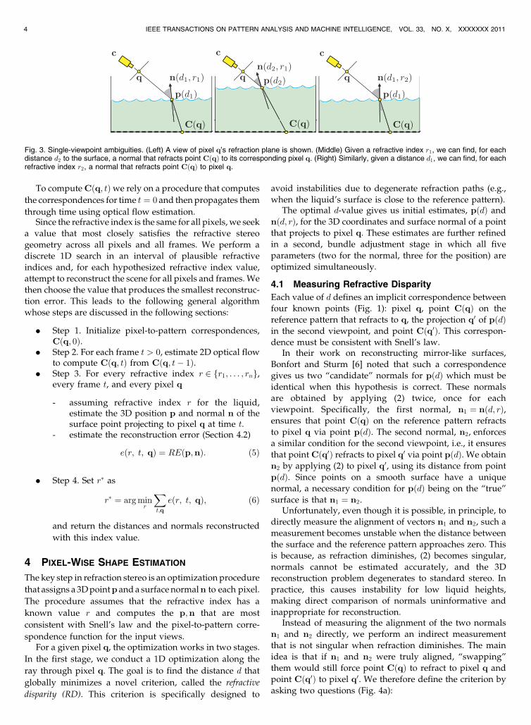
Fig. 3. Single-viewpoint ambiguities. (Left) A view of pixel q’s refraction plane is shown. (Middle) Given a refractive index r1, we can find, for eachdistance d2 to the surface, a normal that refracts point CðqÞ to its corresponding pixel q. (Right) Similarly, given a distance d1, we can find, for eachrefractive index r2, a normal that refracts point CðqÞ to pixel q.

. Suppose the normal at pðdÞ is n2; which point on thereference pattern will refract to q?

. Suppose the normal at pðdÞ is n1; which point on thereference pattern will refract to q0?

Now suppose that points t; t0 are the points that refract to

pixels q;q0, respectively. The distance between t and CðqÞand, similarly, the distance between t0 and Cðq0Þ can be

thought of as a measure of disparity. Intuitively, this distance

tells us how swapping the normals n1;n2 affects consistency

with the available pixel-to-pattern correspondences. To

evaluate a hypothesis d, we simply sum these distances:Refractive Disparity

RDðdÞ ¼ kt�CðqÞk2 þ kt0 �Cðq0Þk2 : ð7Þ

When the distance between the true surface and thereference pattern is large, refractive disparity is equivalent

to a direct measurement of the alignment between vectors

n1;n2, i.e., it is zero if and only if n1 ¼ n2. On the other

hand, as the liquid’s true surface approaches the reference

pattern, refractive disparity diminishes. This is because the

refractive effect of changing a point’s surface orientation

diminishes as well (Fig. 4b). As a result, the minimization

can be applied to any image pixel for which CðqÞ is known,

regardless of whether or not the ray through the pixel

actually intersects the liquid’s surface.To compute point t for a given d value, we trace a ray

from the first viewpoint through pixel q, refract it at

point pðdÞ according to normal n2, and intersect it with the

(known) surface of the reference pattern. Point t0 is

computed in an identical manner. To find the distance d

that globally minimizes refractive disparity along the ray,

we use Matlab’s fminbnd() function, which is based on

golden-section search [44].

4.2 Computing 3D Position and Orientation

Even though refractive disparity minimization yields goodreconstructions in practice, it has two shortcomings. First, it

treats the cameras asymmetrically because optimization

occurs along the ray through one pixel. Second, it only

optimizes the distance along that ray, not the 3D coordi-

nates and orientation of a surface point. We therefore use an

additional step that adjusts all shape parameters (p and n)

in order to minimize a symmetric image reprojection error.

To evaluate the consistency of p and n, we checkwhether the refractions caused by such a point areconsistent with the refractions observed in the input views.In particular, let qp;q

0p be the point’s projections in the two

cameras and suppose that t; t0 are the points on thereference pattern that refract to qp;q

0p, respectively, via

point p. To compute the reprojection error, we measure thedistance between pixels qp;q

0p and the “true” refracted

image of t; t0 (Fig. 4c):

REðp;nÞ ¼ kqp �C�1ðtÞk2 þ kq0p �C�1ðt0Þk2

þ �Gðkp� p0k; �Þ�1;ð8Þ

where C�1ð:Þ denotes the inverse of the pixel-to-patterncorrespondence function, Gð:; �Þ is the Gaussian withstandard deviation �, and p0 is the starting point of theoptimization. The Gaussian term ensures that the optimiza-tion will return a point p whose projection, qp, alwaysremains in the neighborhood of the originally chosen pixel qin Steps 1 and 2 of the Dynamic Refraction Stereo algorithm(Section 3). We used � ¼ 4 and � ¼ 200 for all of ourexperiments. To minimize the RE functional with respect top and n we use the downhill simplex method [44].

5 IMPLEMENTATION DETAILS

5.1 Estimating Pixel-to-Pattern Correspondences

Accurate 3D shape recovery requires knowing the pixel-to-pattern correspondence function Cðq; tÞwith high accuracy.While color-based techniques have been used to estimatethis function for image-based rendering applications [10],they are not appropriate for reconstruction for severalreasons. First, different liquids absorb different wave-lengths by different amounts [49], altering a pattern’sappearance in a liquid-dependent way. Second, since lightabsorption depends on distance traveled within the liquidand since this distance depends on the liquid’s instanta-neous shape, the appearance of the same point on a patternwill change through time. Third, the intensity of lighttransmitted through the surface depends on the Fresneleffect [18] and varies with wavelength and the angle ofincidence. This makes it difficult to use color as a means tolocalize points on a pattern with subpixel accuracy.

In order to avoid these complications, we use amonochrome checkered pattern and rely on corners to

MORRIS AND KUTULAKOS: DYNAMIC REFRACTION STEREO 5

Fig. 4. Optimization criteria for refraction stereo. (a) Measuring refractive disparity. Normals are drawn according to the refractions they produce.(b) For small surface-to-pattern distances, swapping n1 and n2 does not influence the distance between CðqÞ and t significantly. (c) Measuringimage reprojection error at one of the viewpoints.

establish and maintain pixel-to-pattern correspondences(Figs. 5a and 5b). We assume that the liquid’s surface isundisturbed at time t ¼ 0 and use the Harris corner detector[21] to detect corners at subpixel resolution. This gives usthe initial pixel-to-pattern correspondences. To track thelocation of individual corners in subsequent frames whileavoiding drift, we estimate flow between the current frameand the frame at time t ¼ 0, using the flow estimates fromthe previous frame as an initial guess. We compute flowwith a translation-only version of the Lucas-Kanadeinverse-compositional algorithm [3] and use Levenberg-Marquardt minimization to obtain subpixel registration.This algorithm is applied to an 11� 11 pixel neighborhoodaround each corner. We use the registration error returnedby the algorithm as a means to detect failed localizationattempts. In the case of failure, the flow computed for thatcorner is not used and the corner’s previously knownlocation is propagated instead. This allows our tracker toovercome temporary obscurations due to blur, splashes, orextreme refractive distortions (Fig. 5c). The above proce-dure gives values of the correspondence function Cðq; tÞ fora subset of the pixels. To evaluate the function for everypixel, we use bilinear interpolation.

5.2 Fusing 3D Positions and Orientations

Refraction stereo yields a separate 3D position and 3Dnormal for each pixel. While this is a richer shapedescriptor, the problem of reconstructing a single surfacethat is consistent with both types of data is still open. A keydifficulty is that point and normal measurements havedifferent noise properties, and hence a surface computed

via normal integration and a surface computed by fitting amesh to the 3D points will not necessarily agree. As a firststep, we used simulations and ground-truth experiments toestimate the reliability of each data source as a function ofsurface height, i.e., distance from the plane of the referencepattern (Fig. 6). Since reconstructed normals are highlyreliable for large heights, we used this analysis to set aheight threshold below which normals are deemed lessreliable than positions. That portion of the surface isreconstructed from positional data. For the remainingpixels, we reconstruct the surface via normal integrationusing the Ikeuchi-Horn algorithm [27] and merge theresults. In cases where all reconstructed positions are abovethe height threshold, we rely on normal integration tocompute 3D shape and use the average 3D position toeliminate the integrated surface’s height ambiguity.

6 EXPERIMENTAL RESULTS

6.1 Experimental Setup

Fig. 5a shows our setup. The checkered pattern at thebottom of the tank was in direct contact with the water toavoid secondary refractions. During our experiments, thepattern was brightly lit from below to avoid specularreflections and to enable use of a small aperture for thecameras (and hence, a large depth of field). Images wereacquired at a rate of 60 Hz with a pair of synchronizedSony DXC-9000 progressive-scan cameras, whose electro-nic shutter was set to 1/500 sec to avoid motion blur. Bothcameras were approximately 1 meter above the tank

6 IEEE TRANSACTIONS ON PATTERN ANALYSIS AND MACHINE INTELLIGENCE, VOL. 33, NO. X, XXXXXXX 2011

Fig. 5. (a) Experimental setup. (b) Typical close-up view of pattern, seen through water surface. (c) Distorted view, corresponding to tracking failureat the central corners.

Fig. 6. Reconstruction accuracy as a function of water height, for real (dotted line) and simulated (solid line) flat water surfaces. Bars indicate standarddeviation. Simulations are for a 0.08 pixel localization error; in real flat water experiments, corner localization precision was measured to be~0:1 pixels.

bottom and were calibrated using the Matlab CalibrationToolbox [8].

6.2 Simulations

To evaluate the stability of our algorithms, we performedsimulations that closely matched the experimental conditionsin the lab (e.g., relative position of cameras, pattern-to-camera distances, feature localization errors, etc.). Wesimulated the reconstruction error for planar water surfacesas a function of the surface-to-pattern height, and for variouslevels of error in corner localization and camera calibration.We modeled the localization error by perturbing the imagecoordinates of the projected corners by a Gaussian with afixed standard deviation. For each height, we reconstructed10,000 individual points and measured their deviation fromthe ground-truth plane (Fig. 6). These simulations confirmthat the accuracy of reconstructed normals degrades quicklyfor water heights less than 4 mm. Importantly, the accuracy ofdistance computations is not sensitive to variations in waterheight, confirming the stability of our optimization-basedframework for refractive stereo (Section 4.1). We alsocompared the effect of localization error on the results (Fig. 7).

In addition, we ran simulations to test the stability ofrefractive index estimation. We simulated a stationarysinusoidal surface whose average height was 40 mm andwhose amplitude was 2 mm. We then computed the totalreconstruction error for various combinations of true andhypothesized refractive index values (Fig. 8). We used alocalization error of 0.1 pixels for these simulations to reflectour actual experimental conditions. These simulations showthat our objective function has a minimum very close to theexpected refractive index. Also note that the valley aroundthe minimum becomes more shallow as the refractive indexincreases.

6.3 Accuracy Experiments

Since ground truth was not available, we assessed ouralgorithm’s accuracy by applying it to the reconstruction offlat water surfaces whose height from the tank bottomranged from 4 to 15 mm. For each water height, wereconstructed a point p and a normal n independently foreach of 1,836 pixels in the two image planes, giving rise toas many 3D points and normals. No smoothing orpostprocessing was performed. To assess the accuracy ofthe reconstructed points, we fit a plane using least squaresand measured the points’ RMS distance from this plane. Toassess accuracy in the reconstructed normals, we computedthe average normal and measured the mean distance ofeach reconstructed normal from the average normal. Theseresults, also shown in Fig. 6, closely match the behaviorpredicted by our simulations. They suggest that reconstruc-tions are highly precise, with distance variations around0.25 mm (i.e., within 99.97 percent of the surface-to-cameradistance) and normal variations on the order of 2 degreesfor water heights above 8 mm.

6.4 Experiments with Dynamic Surfaces

Figs. 11, 12, and 13 show reconstructions for severaldynamic water surfaces. The experiments test our algor-ithm’s capabilities under a variety of conditions—fromrapidly fluctuating water that is high above the tank bottomto water that is being poured into an empty tank where thewater height is very small and refraction is degenerate ornear-degenerate for many pixels.

Several observations can be made from these experi-ments. First, our tracking-based framework allows us tomaintain accurate pixel-to-pattern correspondences for 100sof frames, enabling dynamic reconstructions that lastseveral seconds. Second, the reconstructed distances remain

MORRIS AND KUTULAKOS: DYNAMIC REFRACTION STEREO 7

Fig. 7. (Left) Reconstruction accuracy as a function of water height for several values of pixel localization error. (Right) Normal reconstruction errorfor the same pixel localization error values.

Fig. 8. Total reconstruction error as a function of hypothesized refractive index r. Simulations are shown for five different ground-truth refractiveindices.

stable despite large variations in water height and areaccurate enough to show fine surface effects, even in caseswhere the total water height never exceeds 6 mm (e.g., the“pour” sequence). Third, the reconstructed normal maps, aspredicted, show fine surface fluctuations at larger heightsbut degrade to noise level for water heights near zero.Qualitatively, when there is sufficient water in the tank,they appear to contain less noise than depth maps. Fourth,our normal integration algorithm seems to oversmooth finesurface details that are clearly present in the depth andnormal maps. This suggests that a more sophisticatedapproach is needed here (e.g., [41]). The following para-graphs discuss our results in more detail.

Ripple sequence (Fig. 11). The ripple sequence shows adrop of water dripping into a tank with approximately25 mm of water in it.3 The drop causes layers of circularwaves to emanate from the point of contact. There are acombination of large and fine-scale waves in the sequence,making for an interesting reconstruction problem. Weachieved a good reconstruction of depth and normals sincethe surface depth provided sufficient refraction for reliablereadings in both categories. The normals provide betterresolution of the fine ripples. The initial splash caused whenthe drop first hits the water produced strong distortions ofthe underlying pattern which our system was unable totrack. We thus reinitialized the system immediately afterthe worst distortions had elapsed and were able to capturethe expanding circular waves.

In the depth maps, errors are more common at points ofgreatest distortion of the ripple, causing sharp peaks (brightor dark spots in Fig. 11). Despite these depth errors, thecorresponding normals appear to be correct and the normalmaps are very smooth, allowing tiny leading ripples to beeasily identified.

Pour sequence (Fig. 12). This sequence shows water beingpoured into an empty tank, spreading across the patternfrom left to right. This sequence tests our system’s ability tocope with water heights that are zero or near zero. Thesequence also exhibits large shape variations due to ripples,as well as bubbles forming on the surface. Our reconstruc-tion successfully handled the height variations usingrefractive disparity: Although reconstructed normals ex-hibited increased noise in the shallow portions, the depthswere reconstructed faithfully. Note that the large regions ofnoise in the normal maps correspond to areas with no water.

Also note that the reconstructed height maps are smooth atthe water edges, suggesting robustness to shallow water.

In areas of nonzero water height, the normal mapsprovide fine detail of the surface, lacking much of the noiseevident in the height maps. For instance, fine waves andripples can be seen in the normal maps at all three timeinstants shown in Fig. 12. By comparison, only the larger-scale waves appear in the height map because noise tends toobscure finer details. Note that while our system is notdesigned to handle bubbles, the reconstruction actuallycaptured indentations corresponding to the bubbles as wellas the ripples forming when they burst (e.g., see the middleof the normal map in the second time instant).

Waves sequence (Fig. 13). This sequence shows wavespropagating from the left to the right on a water surface at aheight of approximately 24 mm. There are several interleav-ing wavefronts of various scales. This sequence provides thegreatest variation in water height and overall roughness.Reconstructions from this data set suffered from morecalibration error and thus exhibit stronger noise. This ismost noticeable in the moire patterns appearing in both thedepth and normal maps. Despite this, we did obtaininteresting reconstructions of the rough water surface. Werecover both the large and small scale wave fronts, which canbe visually tracked across the sequence in the normal maps.

6.5 Refractive Index Determination

In addition to reconstructing both surface and normaldata, our system was able to obtain an estimate of therefractive index of the transparent medium. We ran ouralgorithm on all three sequences of Figs. 11, 12, and 13,over a range of seven frames for each. Fig. 9 shows thetotal reconstruction error corresponding to specific valuesof the refractive index, for the each data set. The curvesexhibit a minimum near the correct refractive index forwater, 1.33, confirming the predictions of Theorem 1. Thisis because Step 4 of our algorithm enforces a very strongglobal constraint: The light path of every pixel at everytime instant and at every viewpoint must be consistentwith the same refractive index value.

7 DISCUSSION

7.1 Ambiguous Surfaces

Although our experimental results suggest that it is possibleto estimate refractive indices from stereo sequences, ageneral question is whether this problem can be ambiguous,i.e., whether two surfaces with different refractive indicescan produce the same observed stereo image pair. Our

8 IEEE TRANSACTIONS ON PATTERN ANALYSIS AND MACHINE INTELLIGENCE, VOL. 33, NO. X, XXXXXXX 2011

Fig. 9. Total reconstruction error as a function of refractive index. (Left) Combined error of several frames from the RIPPLE sequence. (Middle)Combined error of several frames from the POUR sequence. (Right) Combined error of several frames from the WAVES sequence.

3. See the supplemental videos, which can be found on the ComputerSociety Digital Library at http://doi.ieeecomputersociety.org/10.1109/TPAMI.2011.24.

initial analysis, described below, indicates that such pairs ofsurfaces do exist but they do not have a “simple” shape:Indeed, the points on a pair of ambiguous surfaces mustsatisfy a joint system of very complex trigonometricequations for such an ambiguity to exist.

We use a numerical approach to construct point sampleson such surface pairs as follows: Given the refractive index rof the true surface S and the refractive index ra of anambiguous surface R, we construct points and normals thatlie on both S and R. First, we begin with a seed point p1 onS which is imaged at q1 in c (Fig. 10). Then, we find asecond point a1 that lies along the ray from q1 to p1 and onthe ambiguous surface R. The depth of a1 and its normal m1

must be chosen so that the pixel ray refracts to point Cðq1Þon the tank bottom. Next, we project a1 into view c0 andintersect this ray with S to obtain another point p2. Thenormal of p2 must cause the ray through pixel q02 to berefracted toward Cðq02Þ. From our initial seed point, thisprocess gives us two new points: a1 on R and p2 on S. Wecan repeat this process either by adding new seed points orby repeating the above steps with p2 as the seed. Fig. 10ashows this construction repeated twice. Since we have onlyone degree of freedom in the depth/normal of the points piand ai, any ambiguous surface pairs must be highlyconstrained. For instance, if we force the points pi and aito lie on parallel planes, the normals associated with thesepoints cannot both satisfy these constraints and agree withthe global planar normal. Fig. 10b shows two surface pairsconstructed from a sparse set of seeds as described.Intermediate surface points were interpolated according tothe sparse points and their normals.

While the above construction suggests the existence ofambiguous surfaces, these surfaces are not as important inpractice because the scene is dynamic: In our algorithm, asingle refractive index value must account for the refractions

produced by the entire sequence of 3D surfaces of the liquid,not just the 3D surface in a single instant. In fact, refractiveindex estimation exploits the dynamic/statistical nature ofliquids in three ways: 1) The surface is highly variable andhence we observe many different, complex surfaces withthe same refractive index during image acquisition, 2) theirdeforming surface is unlikely to globally match one of the“special” ambiguous shapes, and 3) even if it does, it isunlikely that such a “special” shape will occur for manytime instants. In practice, this allows us to side-step theissue of ambiguities by enforcing refractive index consis-tency with all available data (multiple time instants, evenmultiple acquisition experiments) using our search-basedrefractive index estimation algorithm. Experimentally, thelack of shape-index ambiguities over an acquired data set isconfirmed by error curves that have only one (global)minimum, as in Fig. 9.

7.2 Pixel-to-Pattern Function

In our description of the algorithm and its implementation,we assumed that CðÞwas invertible. We note, however, thatCðÞ can be many-to-one and not generally invertible. Theconditions that cause CðÞ to be invertible were noted byMurase [40], deemed reasonable, and used in his work onliquid reconstruction. From a technical standpoint, how-ever, our analysis does not require CðÞ to be globallyinvertible: All we need is that it is locally invertible, i.e., foralmost all pixels q (in a measure-theoretic sense), therestriction of CðÞ to some open neighborhood of q is aninvertible function. This does permit the occurrence ofisolated singularities (i.e., pixels or image curves where CðÞis not invertible for any neighborhood).

For example, if we were to take a simple 2D scene such as asurface defined by y ¼ cosðxÞwith the camera looking downthe �y axis, CðÞ is not globally invertible. The scene is,however, locally invertible for all values of x except two: For

MORRIS AND KUTULAKOS: DYNAMIC REFRACTION STEREO 9

Fig. 10. (a) Ambiguous surface construction: Points p1, p2, and p3 lie on surface S, points a1 and a2 lie on the ambiguous surface R. Note thatcorrespondence functions Cðq02Þ, Cðq03Þ, Cðq1Þ, and Cðq2Þ all agree with both the true and ambiguous surface points and their normals.(b) Ambiguous surface pairs constructed according to Section 7.1. (Left) The depths of S were chosen to fit a plane. (Right) The depths of S werechosen to fit a sinusoidal surface.

a given refractive index value and a camera located atinfinity, there are only two incoming rays/pixels where localinvertibility breaks down: These rays hit the cosðxÞ curvenear its inflection points, where the mapping from incomingrays to points on the x-axis “folds” onto itself. Moregenerally, the singularities where local invertibility breaksdown have properties analogous to the singularities of theGauss map where, generically, the mapping from surfacepoints to their normals is singular either on parabolic curves,

corresponding to “folds” of the Gauss map, or on isolated

points, corresponding to “cusps” of the map.We also examine in further detail how the flow

propagates from Cðt� 1Þ to CðtÞ. There are two cases:1) The Lucas-Kanade algorithm is able to localize in frame ta corner that was also localized in frame t� 1. In this case,the flow vector assigned to the corner at time t� 1 is itsdisplacement between the two frames. This process iscompletely local and is well defined wherever CðÞ is locally

10 IEEE TRANSACTIONS ON PATTERN ANALYSIS AND MACHINE INTELLIGENCE, VOL. 33, NO. X, XXXXXXX 2011

Fig. 11. RIPPLE sequence. All maps correspond to a top view of the tank and show raw, per-pixel data. The mesh images show a surface fit to thedata scaled by 5 in the vertical axis.

(but perhaps not globally) invertible. 2) The LK algorithmfails to localize the corner at frame t. This does not cause abreakdown of flow estimation for subsequent frames. Inthis case, the algorithm interpolates the flow vectorscomputed at four neighboring corners in frame t� 1 inorder to assign a flow vector to the corner that was lost inframe t. Bilinear interpolation is used, with weightsdetermined by the corners’ distance from each other. Wethen use the position in frame t� 1 of the lost corner and

the interpolated flow vector to assign it a “virtual” position

in frame t. This position is used to initialize the LK

algorithm in frame tþ 1 in an attempt to relocalize the lost

corner. In case of failure at tþ 1, propagation is repeated

until the corner is reacquired. Since these distortions are

local and persist for just few frames, we have found that the

strategy works well in practice and has enabled propaga-

tion of pixel-to-pattern correspondences for 100s of frames.

MORRIS AND KUTULAKOS: DYNAMIC REFRACTION STEREO 11

Fig. 12. POUR sequence. All maps correspond to a top view of the tank and show raw, per-pixel data. The mesh images show a surface fit to thedata scaled by 5 in the vertical axis.

Our current implementation does not check for the

possibility that after a tracking failure (i.e., singularity of

CðÞ), a corner at frame t� 1 appears in more than one

location in frame t (or vice versa). While it is certainly

possible to do so, the sequences we have acquired suggest

that such events are very transient and cause significant

distortions in the local neighborhood of a corner, making it

very hard to localize it, let alone identify multiple images of

it. In such cases, flow propagation allows the corner to be

reacquired when distortions are reduced.

7.3 Optimization

Our focus in this paper has been on the design of

optimization functionals for performing pixel-wise refrac-

tion stereo calculations ((8) and (5)), not on the optimization

process itself. In particular, our exhaustive search over

discretized refraction indices could potentially be replaced

12 IEEE TRANSACTIONS ON PATTERN ANALYSIS AND MACHINE INTELLIGENCE, VOL. 33, NO. X, XXXXXXX 2011

Fig. 13. WAVES sequence. All maps correspond to a top view of the tank and show raw, per-pixel data. The mesh images show a surface fit to thedata scaled by 5 in the vertical axis.

by a golden-section search [17] or by a nonlinear optimiza-

tion procedure that optimizes all points, normals, and

refractive index simultaneously. Similarly, the surface

reconstruction procedure in Section 5.2 is largely heuristic

—a more rigorous approach would be to formulate it as a

global procedure that solves for the entire surface, in the

spirit of recent approaches to multiview stereo [34]. In that

case, the functional REðp;nÞ in (8) would replace the

traditional measures of photo consistency in multiview

stereo.

8 CONCLUDING REMARKS

Liquids can generate extremely complex surface phenom-

ena, including breaking waves, bubbles, and extreme

surface distortions. While our refraction stereo results are

promising, they are just an initial attempt to model liquid

flow in relatively simple cases. Our ongoing work includes1) reconstructing surfaces that produce multiple refractions

[35], 2) reconstructing liquids by exploiting their refractive

and reflective properties (e.g., by also treating them as

mirrors), and 3) “reusing” captured 3D data to create new,

realistic fluid simulations.

ACKNOWLEDGMENTS

This work was supported in part by the Natural Sciences and

Engineering Research Council of Canada under the RGPIN

program, by the Province of Ontario under the OGSST

program, by a fellowship from the Alfred P. Sloan Founda-

tion, and by an Ontario Premier’s Research Excellence

Award. A preliminary version of this work appears in [38].

REFERENCES

[1] Y. Adato, Y. Vasilyev, O. Ben-Shahar, and T. Zickler, “Toward aTheory of Shape from Specular Flow,” Proc. IEEE 11th Int’l Conf.Computer Vision, pp. 1-8, 2007.

[2] S. Agarwal, S.P. Mallick, D. Kriegman, and S. Belongie, “OnRefractive Optical Flow,” Proc. Eighth European Conf. ComputerVision, pp. 483-494, 2004.

[3] S. Baker and I. Matthews, “Lucas-Kanade 20 Years On: A UnifyingFramework,” Int’l J. Computer Vision, vol. 56, no. 3, pp. 221-255,2004.

[4] M. Ben-Ezra and S. Nayar, “What Does Motion Reveal aboutTransparency?” Proc. Ninth Int’l Conf. Computer Vision, pp. 1025-1032, 2003.

[5] A. Blake, “Specular Stereo,” Proc. Int’l Joint Conf. ArtificialIntelligence, pp. 973-976, 1985.

[6] T. Bonfort and P. Sturm, “Voxel Carving for Specular Surfaces,”Proc. Ninth Int’l Conf. Computer Vision, pp. 591-596, 2003.

[7] T. Bonfort, P. Sturm, and P. Gargallo, “General Specular SurfaceTriangulation,” Proc. Asian Conf. Computer Vision, pp. 872-881, 2006.

[8] J.-Y. Bouguet, “MATLAB Camera Calibration Toolbox,” http://www.vision.caltech.edu/bouguetj/calib_doc/, 2010.

[9] T. Chen, M. Goesele, and H.-P. Seidel, “Mesostructure fromSpecularity,” Proc. 2006 IEEE CS Conf. Computer Vision and PatternRecognition, vol. 2, pp. 1825-1832, 2006.

[10] Y.-Y. Chuang, D.E. Zonkger, J. Hirdorff, B. Curless, and D.H.Salesin, “Environment Matting Extensions: Toward HigherAccuracy and Real-Time Capture,” Proc. ACM SIGGRAPH,pp. 121-130, 2000.

[11] J.M. Daida, D. Lund, C. Wolf, G.A. Meadows, K. Schroeder, J.Vesecky, D.R. Lyzenga, B.C. Hannan, and R.R. Bertram, “Measur-ing Topography of Small-Scale Water Surface Waves,” Proc.Geoscience and Remote Sensing Symp. Conf., vol. 3, pp. 1881-1883,1995.

[12] Y. Ding and J. Yu, “Recovering Shape Characteristics on Near-FlatSpecular Surfaces,” Proc. IEEE Conf. Computer Vision and PatternRecognition, pp. 1-8, 2008.

[13] Y. Ding, J. Yu, and P. Sturm, “Recovering Specular Surfaces UsingCurved Line Images,” Proc. IEEE Conf. Computer Vision and PatternRecognition, June 2009.

[14] D. Enright, S. Marschner, and R. Fedkiw, “Animation andRendering of Complex Water Surfaces,” Proc. ACM SIGGRAPH,pp. 736-744, 2002.

[15] P. Flach and H.-G. Maas, “Vision-Based Techniques for RefractionAnalysis in Applications of Terrestrial Geodesy,” Proc. Int’lArchives of Photogrammetry and Remote Sensing, pp. 195-201, 2000.

[16] Y. Francken, T. Cuypers, T. Mertens, J. Gielis, and P. Bekaert,“High Quality Mesostructure Acquisition Using Specularities,”Proc. IEEE Conf. Computer Vision and Pattern Recognition, pp. 1-7,June 2008.

[17] C.B. Moler, G.E. Forsyth, and M.A. Malcom, Computer Methods forMathematical Computations. Prentice Hall, 1976.

[18] A.S. Glassner, Principles of Digital Image Synthesis. MorganKaufmann, 1995.

[19] M.A. Halstead, B.A. Barsky, S.A. Klein, and R.B. Mandell,“Reconstructing Curved Surfaces from Specular Reflection Pat-terns Using Spline Surface Fitting of Normals,” Proc. ACMSIGGRAPH, pp. 335-342, 1996.

[20] F.H. Harlow and J.E. Welch, “Numerical Calculation of Time-Dependent Viscous Incompressible Flow,” Physics of Fluids, vol. 8,pp. 2182-2189, 1965.

[21] C. Harris and M. Stephens, “A Combined Edge and CornerDetector,” Proc. Fourth Alvey Vision Conf., pp. 189-192, 1988.

[22] R.I. Hartley and A. Zisserman, Multiple View Geometry in ComputerVision. Cambridge Univ. Press, 2000.

[23] R.I. Hartley and P. Sturm, “Triangulation,” Computer Vision andImage Understanding, vol. 68, no. 2, pp. 146-157, 1997.

[24] J. Hohle, “Reconstruction of the Underwater Object,” Proc.Photogrammetric Eng., pp. 948-954, 1971.

[25] M.B. Hullin, M. Fuchs, I. Ihrke, H.-P. Seidel, and H.P.A. Lensch,“Fluorescent Immersion Range Scanning,” ACM Trans. Graphics,vol. 27, no. 3, pp. 87-1-87-10, Aug. 2008.

[26] K. Ikeuchi, “Determining the Surface Orientations of SpecularSurfaces by Using the Photometric Stereo Method,” IEEE Trans.Pattern Analysis Machine Intelligence, vol. 3, no. 6, pp. 661-669, Nov.1981.

[27] K. Ikeuchi and B.K.P. Horn, “Numerical Shape from Shading andOccluding Boundaries,” Artificial Intelligence, vol. 17, pp. 141-184,1981.

[28] B. Jahne, J. Klinke, P. Geissler, and F. Hering, “Image SequenceAnalysis of Ocean Wind Waves,” Proc. Int’l Seminar on Imaging inTransport Processes, 1992.

[29] B. Jahne, J. Klinke, and S. Waas, “Imaging of Short Ocean WindWaves: A Critical Theoretical Review,” J. Optical Soc. Am. A,vol. 11, no. 8, pp. 2197-2209, 1994.

[30] B. Jahne, M. Schmidt, and R. Rocholz, “Combined Optical Slope/Height Measurements of Short Wind Waves: Principle andCalibration,” Measurement Science and Technology, vol. 16, no. 10,pp. 1937-1944, 2005.

[31] J. Kaminski, S. Lowitzsch, M.C. Knauer, and G. Hausler, “Full-Field Shape Measurement of Specular Surfaces,” Proc. Fifth Int’lWorkshop Automatic Processing of Fringe Patterns, 2005.

[32] W.C. Keller and B.L. Gotwols, “Two-Dimensional Optical Mea-surement of Wave Slope,” Applied Optics, vol. 22, no. 22, pp. 3476-3478, 1983.

[33] J.J. Koenderink and A.J. van Doorn, “The Structure of Two-Dimensional Scalar Fields with Applications to Vision,” BiologicalCybernetics, vol. 33, pp. 151-158, 1979.

[34] K. Kolev, M. Klodt, T. Brox, and D. Cremers, “Continuous GlobalOptimization in Multiview 3d Reconstruction,” Int’l J. ComputerVision, vol. 84, no. 1, pp. 80-96, 2009.

[35] K.N. Kutulakos and E. Steger, “A Theory of and Refractive andSpecular 3d Shape by Light-Path Triangulation,” Proc. 10th Int’lConf. Computer Vision, pp. 1448-1455, 2005.

[36] F. Losasso, F. Gibou, and R. Fedkiw, “Simulating Water andSmoke with an Octree Data Structure,” ACM Trans. Graphics,vol. 23, no. 3, pp. 457-462, 2004.

[37] H.-G. Maas, “New Developments in Multimedia Photogramme-try,” Optical 3D Measurement Techniques III. Wichmann Verlag,1995.

MORRIS AND KUTULAKOS: DYNAMIC REFRACTION STEREO 13

[38] N. Morris and K.N. Kutulakos, “Dynamic Refraction Stereo,” Proc.10th Int’l Conf. Computer Vision, pp. 1573-1580, 2005.

[39] M. Muller, D. Charypar, and M. Gross, “Particle-Based FluidSimulation for Interactive Applications,” Proc. 2003 ACM SIG-GRAPH/Eurographics Symp. Computer Animation, pp. 154-159, 2003.

[40] H. Murase, “Surface Shape Reconstruction of an UndulatingTransparent Object,” Proc. Third Int’l Conf. Computer Vision,pp. 313-317, 1990.

[41] D. Nehab, S. Rusinkiewicz, J. Davis, and R. Ramamoorthi,“Efficiently Combining Positions and Normals for Precise 3DGeometry,” Proc. ACM SIGGRAPH, pp. 536-543, 2005.

[42] A. Okamoto, “Orientation Problem of Two-Media Photographswith Curved Boundary Surfaces,” Proc. Photogrammetric Eng. andRemote Sensing, pp. 303-316, 1984.

[43] M. Oren and S.K. Nayar, “A Theory of Specular SurfaceGeometry,” Proc. Fifth Int’l Conf. Computer Vision, pp. 740-747,1995.

[44] W.H. Press, B.P. Flannery, S.A. Teukolsky, and W.T. Vetterling,Numerical Recipies in C. Cambridge Univ. Press, 1988.

[45] A.C. Sanderson, L.E. Weiss, and S.K. Nayar, “Structured High-light Inspection of Specular Surfaces,” IEEE Trans. Pattern AnalysisMachine Intelligence, vol. 10, no. 1, pp. 44-55, Jan. 1988.

[46] S. Savarese and P. Perona, “Local Analysis for 3D Reconstructionof Specular Surfaces—Part II,” Proc. Seventh European Conf.Computer Vision, pp. 759-774, 2002.

[47] H. Schultz, “Retrieving Shape Information from Multiple Imagesof a Specular Surface,” IEEE Trans. Pattern Analysis and MachineIntelligence, vol. 16, no. 2, pp. 195-201, Feb. 1994.

[48] O.H. Shemdin, “Measurement of Short Surface Waves withStereophotography,” Proc. Eng. in the Ocean Environment Conf.,pp. 568-571, 1990.

[49] S.A. Sullivan, “Experimental Study of the Absorption in DistilledWater, Artificial Sea Water, and Heavy Water in the VisibleRegion of the Spectrum,” J. Optical Soc. Am., vol. 53, pp. 962-968,1963.

[50] M. Tarini, H.P.A. Lensch, M. Goesele, and H.-P. Seidel, “3DAcquisition of Mirroring Objects,” Technical Report MPI-I-2003-4-001, Max Planck Institut fur Informatik, 2003.

[51] T. Treibitz, Y.Y. Schechner, and H. Singh, “Flat RefractiveGeometry,” Proc. IEEE Conf. Computer Vision and Pattern Recogni-tion, pp. 1-8, 2008.

[52] B. Trifonov, D. Bradley, and W. Heidrich, “TomographicReconstruction of Transparent Objects,” Proc. 17th EurographicsSymp. Rendering, pp. 51-60, 2006.

[53] B. Triggs, P.F. McLauchlan, R.I. Hartley, and A.W. Fitzgibbon,“Bundle Adjustment—A Modern Synthesis,” Proc. Int’l WorkshopVision Algorithms, pp. 298-372, 2000.

[54] Y. Vasilyev, Y. Adato, T. Zickler, and O. Ben-Shahar, “DenseSpecular Shape from Multiple Specular Flows,” Proc. IEEE Conf.Computer Vision and Pattern Recognition, pp. 1-8, 2008.

[55] J. Wang and K.J. Dana, “Relief Texture from Specularities,” IEEETrans. Pattern Analysis Machine Intelligence, vol. 28, no. 3, pp. 446-457, Mar. 2006.

[56] Z. Wu and G.A. Meadows, “2-D Surface Reconstruction of WaterWaves,” Proc. Eng. in the Ocean Environment. Conf., pp. 416-421,1990.

[57] L. Zhang, N. Snavely, B. Curless, and S.M. Seitz, “Spacetime Faces:High Resolution Capture for Modeling and Animation,” ACMTrans. Graphics, vol. 23, no. 3, pp. 548-558, 2004.

[58] X. Zhang and C.S. Cox, “Measuring the Two-DimensionalStructure of a Wavy Water Surface Optically: A Surface GradientDetector,” Experiments in Fluids, vol. 17, pp. 225-237, 1994.

[59] L. Zhou, C. Kambhamettu, and D.B. Goldgof, “Fluid Structure andMotion Analysis from Multi-Spectrum 2D Cloud Image Se-quences,” Proc. IEEE Conf. Computer Vision and Pattern Recognition,vol. 2, pp. 744-751, 2000.

Nigel J.W. Morris received the BScH degree incomputing and information science fromQueen’s University, Canada, in 2002, and theMSc and PhD degrees in computer science fromthe University of Toronto in 2004 and 2010,respectively. He has worked at MitsubishiElectric Research Labs and is currently leadcomputer scientist at Morgan Solar Inc.

Kiriakos N. Kutulakos received the BA degreein computer science from the University of Crete,Greece, in 1988, and the MS and PhD degrees incomputer science from the University of Wiscon-sin-Madison in 1990 and 1994, respectively.Following his dissertation work, he joined theUniversity of Rochester, where he was a USNational Science Foundation (NSF) postdoctoralfellow and later an assistant professor until 2001.He is currently a professor of computer science

at the University of Toronto. He won the Best Student Paper Award atCVPR ’94, the David Marr Prize in 1999, a David Marr Prize HonorableMention in 2005, and a Best Paper Honorable Mention at ECCV ’06. Heis the recipient of a CAREER award from the US National ScienceFoundation, a Premier’s Research Excellence Award from the govern-ment of Ontario, and an Alfred P. Sloan Research Fellowship. He was anassociate editor of the IEEE Transactions on Pattern Analysis andMachine Intelligence from 2005 to 2010, a program cochair of CVPR ’03and ICCP ’10, and will serve as program cochair of ICCV ’13. He is amember of the IEEE.

. For more information on this or any other computing topic,please visit our Digital Library at www.computer.org/publications/dlib.

14 IEEE TRANSACTIONS ON PATTERN ANALYSIS AND MACHINE INTELLIGENCE, VOL. 33, NO. X, XXXXXXX 2011