IEEE TRANSACTIONS ON PATTERN ANALYSIS AND MACHINE ... · PDF fileEfficient Human Pose...

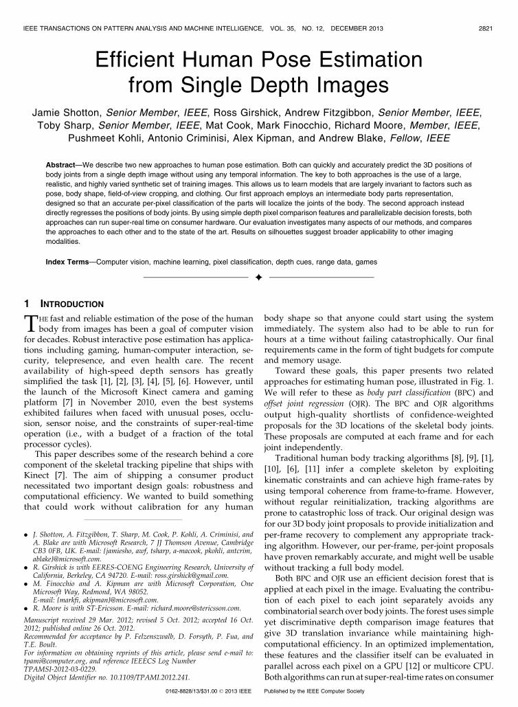
Efficient Human Pose Estimationfrom Single Depth Images

Jamie Shotton, Senior Member, IEEE, Ross Girshick, Andrew Fitzgibbon, Senior Member, IEEE,

Toby Sharp, Senior Member, IEEE, Mat Cook, Mark Finocchio, Richard Moore, Member, IEEE,

Pushmeet Kohli, Antonio Criminisi, Alex Kipman, and Andrew Blake, Fellow, IEEE

Abstract—We describe two new approaches to human pose estimation. Both can quickly and accurately predict the 3D positions of

body joints from a single depth image without using any temporal information. The key to both approaches is the use of a large,

realistic, and highly varied synthetic set of training images. This allows us to learn models that are largely invariant to factors such as

pose, body shape, field-of-view cropping, and clothing. Our first approach employs an intermediate body parts representation,

designed so that an accurate per-pixel classification of the parts will localize the joints of the body. The second approach instead

directly regresses the positions of body joints. By using simple depth pixel comparison features and parallelizable decision forests, both

approaches can run super-real time on consumer hardware. Our evaluation investigates many aspects of our methods, and compares

the approaches to each other and to the state of the art. Results on silhouettes suggest broader applicability to other imaging

modalities.

Index Terms—Computer vision, machine learning, pixel classification, depth cues, range data, games

Ç

1 INTRODUCTION

THE fast and reliable estimation of the pose of the humanbody from images has been a goal of computer vision

for decades. Robust interactive pose estimation has applica-tions including gaming, human-computer interaction, se-curity, telepresence, and even health care. The recentavailability of high-speed depth sensors has greatlysimplified the task [1], [2], [3], [4], [5], [6]. However, untilthe launch of the Microsoft Kinect camera and gamingplatform [7] in November 2010, even the best systemsexhibited failures when faced with unusual poses, occlu-sion, sensor noise, and the constraints of super-real-timeoperation (i.e., with a budget of a fraction of the totalprocessor cycles).

This paper describes some of the research behind a corecomponent of the skeletal tracking pipeline that ships withKinect [7]. The aim of shipping a consumer productnecessitated two important design goals: robustness andcomputational efficiency. We wanted to build somethingthat could work without calibration for any human

body shape so that anyone could start using the systemimmediately. The system also had to be able to run forhours at a time without failing catastrophically. Our finalrequirements came in the form of tight budgets for computeand memory usage.

Toward these goals, this paper presents two related

approaches for estimating human pose, illustrated in Fig. 1.

We will refer to these as body part classification (BPC) and

offset joint regression (OJR). The BPC and OJR algorithms

output high-quality shortlists of confidence-weighted

proposals for the 3D locations of the skeletal body joints.

These proposals are computed at each frame and for each

joint independently.Traditional human body tracking algorithms [8], [9], [1],

[10], [6], [11] infer a complete skeleton by exploiting

kinematic constraints and can achieve high frame-rates by

using temporal coherence from frame-to-frame. However,

without regular reinitialization, tracking algorithms are

prone to catastrophic loss of track. Our original design was

for our 3D body joint proposals to provide initialization and

per-frame recovery to complement any appropriate track-

ing algorithm. However, our per-frame, per-joint proposals

have proven remarkably accurate, and might well be usable

without tracking a full body model.Both BPC and OJR use an efficient decision forest that is

applied at each pixel in the image. Evaluating the contribu-

tion of each pixel to each joint separately avoids any

combinatorial search over body joints. The forest uses simple

yet discriminative depth comparison image features that

give 3D translation invariance while maintaining high-

computational efficiency. In an optimized implementation,

these features and the classifier itself can be evaluated in

parallel across each pixel on a GPU [12] or multicore CPU.

Both algorithms can run at super-real-time rates on consumer

IEEE TRANSACTIONS ON PATTERN ANALYSIS AND MACHINE INTELLIGENCE, VOL. 35, NO. 12, DECEMBER 2013 2821

. J. Shotton, A. Fitzgibbon, T. Sharp, M. Cook, P. Kohli, A. Criminisi, andA. Blake are with Microsoft Research, 7 JJ Thomson Avenue, CambridgeCB3 0FB, UK. E-mail: {jamiesho, awf, tsharp, a-macook, pkohli, antcrim,ablake}@microsoft.com.

. R. Girshick is with EERES-COENG Engineering Research, University ofCalifornia, Berkeley, CA 94720. E-mail: [email protected].

. M. Finocchio and A. Kipman are with Microsoft Corporation, OneMicrosoft Way, Redmond, WA 98052.E-mail: {markfi, akipman}@microsoft.com.

. R. Moore is with ST-Ericsson. E-mail: [email protected].

Manuscript received 29 Mar. 2012; revised 5 Oct. 2012; accepted 16 Oct.2012; published online 26 Oct. 2012.Recommended for acceptance by P. Felzenszwalb, D. Forsyth, P. Fua, andT.E. Boult.For information on obtaining reprints of this article, please send e-mail to:[email protected], and reference IEEECS Log NumberTPAMSI-2012-03-0229.Digital Object Identifier no. 10.1109/TPAMI.2012.241.

0162-8828/13/$31.00 � 2013 IEEE Published by the IEEE Computer Society

hardware, leaving sufficient computational resources toallow complex game logic and graphics to run in parallel.

The two methods also share their use of a very large,realistic, synthetic training corpus, generated by renderingdepth images of humans. Each render is assigned randomlysampled parameters including body shape, size, pose, sceneposition, and so on. We can thus quickly and cheaplygenerate hundreds of thousands of varied images with

associated ground-truth (the body part label images and theset of 3D body joint positions). This allows us to train deepforests, without the risk of overfitting, that can naturallyhandle a full range of human body shapes undergoinggeneral body motions [13], self-occlusions, and posescropped by the image frame.

BPC, originally published in [14], was inspired by recentobject recognition work that divides objects into parts(e.g., [15], [16], [17], [5]). BPC uses a randomized classification

forest to densely predict discrete body part labels across theimage. Given the strong depth image signal, no pairwiseterms or CRF have proven necessary for accurate labeling.The pattern of these labels is designed such that the partsare spatially localized near skeletal joints of interest. Giventhe depth image and the known calibration of the depthcamera, the inferred per-pixel label probabilities can bereprojected to define a density over 3D world space. OJR[18] instead employs a randomized regression forest todirectly cast a set of 3D offset votes from each pixel to thebody joints. These votes are used to again define a worldspace density. Modes of these density functions can befound using mean shift [19] to give the final set of 3D bodyjoint proposals. Optimized implementations of our algo-rithms can run at around 200 frames per second on

consumer hardware, at least one order of magnitude faster

than existing approaches.To validate our algorithms, we evaluate on both real and

synthetic depth images containing challenging poses of a

varied set of subjects. Even without exploiting temporal or

kinematic constraints, the 3D body joint proposals are both

accurate and stable. We investigate the effect of several

training parameters and show a substantial improvement

over the state of the art. Further, preliminary results on

silhouette images suggest more general applicability of our

approach to scenarios where depth cameras are not available.

1.1 Contributions

Our main contribution are as follows:

. We demonstrate that using efficient machine learn-ing approaches, trained with a large-scale, highlyvaried, synthetic training set, allows one to accu-rately predict the positions of the human body jointsin super-real time.

. We show how a carefully designed pattern of bodyparts can transform the hard problem of poseestimation into an easier problem of per-pixelsemantic segmentation.

. We examine both classification and regressionobjective functions for training the decision forests,and obtain slightly surprising results that suggest alimitation of the standard regression objective.

. We employ regression models that compactlysummarize the pixel-to-joint offset distributions atleaf nodes. We show that these make our methodboth faster and more accurate than Hough Forests[20]. We will refer to this as “vote compression.”

This paper builds on our earlier publications [14], [18]. It

unifies the notation, explains the approaches in more detail,

and includes a considerably more thorough experimental

validation.

1.2 Depth Imaging

Depth imaging technology has advanced dramatically over

the last few years, and has finally reached a consumer price

point [7]. Pixels in a depth image indicate the calibrated

distance in meters of 3D points in the world from the

imaging plane, rather than a measure of intensity or color.

We employ the Kinect depth camera (and simulations

thereof) to provide our input data. Kinect uses structured

infrared light and can infer depth images with high spatial

and depth resolution at 30 frames per second.Using a depth camera gives several advantages for

human pose estimation. Depth cameras work in low light

conditions (even in the dark), help remove ambiguity in

scale, are largely color and texture invariant, and resolve

silhouette ambiguities. They also greatly simplify the task of

background subtraction, which we assume in this work as a

preprocessing step. Most importantly for our approach,

since variations in color and texture are not imaged, it is

much easier to synthesize realistic depth images of people

and thus cheaply build a large training dataset.

2822 IEEE TRANSACTIONS ON PATTERN ANALYSIS AND MACHINE INTELLIGENCE, VOL. 35, NO. 12, DECEMBER 2013

Fig. 1. Method overview on ground truth example. BPC first predicts a(color-coded) body part label at each pixel, and then uses these inferredlabels to localize the body joints. OJR instead more directly regressesthe positions of the joints. The input depth point cloud is shown overlaidon the body joint positions for reference.

1.3 Related Work

Human pose estimation has generated a vast literature,surveyed in [21], [22]. We briefly review some of the recentadvances.

1.3.1 Recognition in Parts

Several methods have investigated using some notionof distinguished body parts. One popular technique,pictorial structures [23], was applied by Felzenszwalband Huttenlocher [24] to efficiently estimate human poseby representing the body by a collection of parts arrangedin a deformable configuration. Springs are used betweenparts to model the deformations. Ioffe and Forsyth [25]group parallel edges as candidate body segments andprune combinations of segments using a projected classi-fier. Ramanan and Forsyth [26] find candidate bodysegments as pairs of parallel lines and cluster theirappearances across frames, connecting up a skeleton basedon kinematic constraints. Sigal et al. [9] used eigen-appearance template detectors for head, upper arms, andlower legs proposals. Nonparametric belief propagationwas then used to infer whole body pose. Tu’s “auto-context” was used in [27] to obtain a coarse body partlabeling. These labels were not defined to localize joints,and classifying each frame took about 40 seconds.“Poselets” that form tight clusters in both 3D pose and2D image appearance, detectable using SVMs, werepresented by Bourdev and Malik [17]. Wang and Popovi�c[10] proposed a related approach to track a hand clothed ina colored glove; our BPC system could be viewed asautomatically inferring the colors of a virtual colored suitfrom a depth image. As detailed below, our BPC algorithm[14] extends the above techniques by using parts thatdensely cover the body and directly localize body joints.

1.3.2 Pose from Depth

Recent work has exploited improvements in depth imagingand 3D input data. Anguelov et al. [28] segment puppetsin 3D range scan data into head, limbs, torso, andbackground using spin images and an MRF. Grest et al.[1] use Iterated Closest Point (ICP) to track a skeleton of aknown size and starting position from depth images. In [3],Zhu and Fujimura build heuristic detectors for coarseupper body parts (head, torso, arms) using a linearprogramming relaxation, but require a T-pose initializationto calibrate the model shape. Siddiqui and Medioni [4]hand-craft head, hand, and forearm detectors, and showthat data-driven MCMC model fitting outperforms the ICPalgorithm. Kalogerakis et al. [29] classify and segmentvertices in a full closed 3D mesh into different parts, but donot deal with occlusions and are sensitive to meshtopology. Plagemann et al. [5] build a 3D mesh to findgeodesic extrema interest points which are classified intothree parts: head, hand, and foot. This method providesboth a location and orientation estimate of these parts, butdoes not distinguish left from right, and the use of interestpoints limits the choice of parts.

1.3.3 Regression

Regression has been a staple of monocular 2D human poseestimation [30], [31], [32], [13]. Several methods haveexplored matching exemplars or regressing from a small

set of nearest neighbors. The shape context descriptor wasused by Mori and Malik [33] to retrieve exemplars.Shakhnarovich et al. [34] estimate upper body pose,interpolating k-NN poses efficiently indexed by parametersensitive hashing. Agarwal and Triggs [30] learn aregression from kernelized image silhouette features topose. Navaratnam et al. [32] use the marginal statistics ofunlabeled data to improve pose estimation. Local mixturesof Gaussian Processes were used by Urtasun and Darrell[13] to regress human pose. Our OJR approach combinessome ideas from these approaches with the tools of high-speed object recognition based on decision trees.

1.3.4 Other Approaches

An alternative random forest-based method for poseestimation was proposed by [35]. Their approach quantizesthe space of rotations and gait cycle, though it does notdirectly produce a detailed pose estimate.

A related technique to our OJR algorithm is used inobject localization. For example, in the implicit shapemodel (ISM) [36], visual words are used to learn votingoffsets to predict 2D object centers. ISM has been extendedin two pertinent ways. Muller and Arens [37] apply ISM tobody tracking by learning separate offsets for each bodyjoint. Gall and Lempitsky [20] replace the visual wordcodebook of ISM by learning a random forest in whicheach tree assigns every image pixel to a decision-tree leafnode at which is stored a potentially large collection ofvotes. This removes the dependence of ISM on repeatablefeature extraction and quantization, as well as the some-what arbitrary intermediate codebook representation.Associating a collection of “vote offsets” with each leafnode/visual word, these methods then accumulate votes todetermine the object centers/joint positions. Our OJR

method builds on these techniques by compactly summar-izing the offset distributions at the leaf nodes, learning themodel hyper-parameters, and using a continuous test-timevoting space.

1.4 Outline

The remainder of the paper is organized as follows: Section 2explains how we generate the large, varied training set thatis the key to our approach. Following that, Section 3describes the two algorithms in a unified framework. Ourexperimental evaluation is detailed in Section 4, and weconclude in Section 5.

2 DATA

Many techniques for pose estimation require trainingimages with high-quality ground truth labels, such as jointpositions. For real images, these labels can be veryexpensive to obtain. Much research has thus focused ontechniques to overcome lack of training data by usingcomputer graphics [34], [38], [39], but there are twopotential problems:

1. Rendering realistic intensity images is hampered bythe huge color and texture variability induced byclothing, hair, and skin, often meaning that the dataare reduced to 2D silhouettes [30]. While depthcameras significantly reduce this difficulty, consid-erable variation in body and clothing shape remains.

SHOTTON ET AL.: EFFICIENT HUMAN POSE ESTIMATION FROM SINGLE DEPTH IMAGES 2823

2. Synthetic body pose renderers use, out of necessity,real motion capture (mocap) data. Although techni-ques exist to simulate human motion (e.g., [40]), theydo not yet produce a full range of volitional motionsof a human subject.

In this section, we describe how we overcome theseproblems. We take real mocap data, retarget this to a varietyof base character models, and then synthesize a large,varied dataset. We believe the resulting dataset to con-siderably advance the state of the art in both scale andvariety, and will demonstrate the importance of such a largedataset in our evaluation.

2.1 Motion Capture Data

As noted above, simulating human pose data is an unsolvedproblem. Instead, we obtain ground truth pose data usingmarker-based motion capture of real human actors. Thehuman body is capable of an enormous range of poses.Modeled jointly, the number of possible poses is exponentialin the number of articulated joints. We cannot thus record allpossible poses. However, there is hope. As will be seen inSection 3, our algorithms, based on sliding window decisionforests, were designed to only look at a local neighborhoodof a pixel. By looking at local windows, we factor wholebody poses into combinations of local poses, and can thusexpect the forests to generalize somewhat to unseen poses. Inpractice, even a limited corpus of mocap data where, forexample, each limb separately moves through a wide rangeof poses has proven sufficient. Further, we need not recordmocap with variation in rotation about the vertical axis,mirroring left-right, scene position, body shape, and size, orcamera pose, all of which can be simulated. Given our coreentertainment scenario, we recorded 500 K frames in a fewhundred sequences of driving, dancing, kicking, running,navigating menus, and so on.

To create training data we render single, static depthimages because, as motivated above, our algorithmsdeliberately eschew temporal information. Often, changesin pose from one mocap frame to the next are so small as tobe insignificant. We can thus discard many similar,redundant poses using “furthest neighbor” clustering [41].We represent a pose P as a collection P ¼ ðp1; . . . ;pJÞ ofJ joints where each pj is a 3D position vector. Starting withset Pall of all the recorded mocap poses, we choose an initialpose at random and then greedily grow a set P as

P :¼ P [�

argmaxP2PallnP

minP 02P

dposeðP; P 0Þ�; ð1Þ

where as the distance between poses we use the maximumeuclidean distance over body joints j:

dposeðP; P 0Þ ¼ maxj2f1;...;Jg

��pj � p0j��

2: ð2Þ

We stop growing setPwhen there exists no unchosen posePwhich has dposeðP; P 0Þ > Dpose for any chosen pose P 0. Weset Dpose ¼ 5 cm. This results in a final subset P � Pall

containing approximately 100 K most dissimilar poses.We found it necessary to iterate the process of motion

capture, rendering synthetic training data, training theclassifier, and testing joint prediction accuracy. Thisallowed us to refine the mocap database with regions of

pose space that had been previously missed out. Our earlyexperiments employed the CMU mocap database [42]which gave acceptable results though it covers far less ofpose space.

2.2 Rendering Synthetic Data

We build a randomized rendering pipeline. This can beviewed as a generative model from which we can samplefully labeled training images of people. Our goals inbuilding this pipeline were twofold: Realism—we want thesamples to closely resemble real images so that thelearned model can work well on live camera input; andVariety—the dataset must contain good coverage of theappearance variations we hope to recognize at test time.Fig. 3 illustrates the huge space of possible appearancevariations we need to deal with for just one body part,even when restricted to a pixel’s local neighborhood asdiscussed above.

Our features achieve 3D translation invariance bydesign (see below). However, other invariances such aspose and shape cannot be designed so easily or efficiently,and must instead be encoded implicitly through thetraining data. The rendering pipeline thus randomlysamples a set of parameters, using the best approxima-tions we could reasonably achieve to the variations weexpected to observe in the real world. While we cannothope to sample all possible combinations of variations, ifsamples contain somewhat independent variations (inparticular, excluding artificial correlations such as thinpeople always wear a hat), we can expect the classifier tolearn a large degree of invariance. Let us run through thevariations we simulate:

Base character. We use 3D models of 15 varied basecharacters, both male and female, from child to adult, shortto tall, and thin to fat. Some examples are shown in Fig. 4. Agiven render will pick uniformly at random from thecharacters.

Pose. Having discarded redundant poses from the mocapdata, we retarget the remaining poses P 2 P to each basecharacter using [43]. A pose is selected uniformly at randomand mirrored left-right with probability 1

2 to prevent a left orright bias.

Rotation and translation. The character is rotated about thevertical axis and translated in the scene, uniformly atrandom. Translation ensures we obtain cropped trainingexamples where the character is only partly in-frame.

Hair and clothing. We add mesh models of several hairstyles and items of clothing chosen at random. A slightgender bias is used so that, for instance, long hair is chosenmore often for the female models, and beards are onlychosen for the male models.

Weight and height variation. The base characters alreadyinclude a wide variety of weights and heights. To addfurther variety we add an extra variation in height(�10 percent) and weight (�10 percent). For renderingefficiency, we assume this variation does not affect the poseretargeting.

Camera position and orientation. The camera height, pitch,and roll are chosen uniformly at random within a rangebelieved to be representative of an entertainment scenarioin a home living room.


Camera noise. While depth camera technology hasimproved rapidly in the last few years, real depth camerasexhibit noise, largely due to non-IR-reflecting materials(e.g., glass, hair), surfaces that are almost perpendicularto the sensor, and ambient illumination. To ensure highrealism in our dataset, we thus add artificial noise to theclean computer graphics renders to simulate the depthimaging process: dropped-out pixels, depth shadows, spotnoise, and disparity quantization.

We use standard linear skinning techniques fromcomputer graphics to animate the chosen 3D mesh modelgiven the chosen pose, and a custom pixel shader is used torender the depth images. Fig. 2 compares the varied outputof the pipeline to hand-labeled real depth images. Thesynthetic data is used both as fully labeled training data,and, alongside real hand-labeled depth images, as test datain our evaluation.

In building this randomized rendering pipeline, weattempted to fit as much variety in as many ways as wecould, given the time constraints we were under.Investigating the precise effects of the choice and amountsof variation would be fascinating, but lies beyond thescope of this work.

2.3 Training Data Labeling

A major advantage of using synthetic training images is thatthe ground truth labels can be generated almost for free,allowing one to scale up supervised learning to very largescales. The complete rendering pipeline allows us to rapidlysample hundreds of thousands of unique images of people.The particular tasks we address in this work, BPC and OJR,require different types of label, described next.

2.3.1 BPC labels

Our first algorithm, BPC, aims to predict a discrete bodypart label at each pixel. At training time, these labels arerequired for all pixels, and we thus represent the labels as acolor-coded body part label image that accompanies eachdepth image (see Figs. 1 and Figs. 2).

The use of an intermediate body part representation thatcan localize 3D body joints is a key contribution of thiswork. It transforms the pose estimation problem into onethat can readily be solved by efficient classificationalgorithms. The particular pattern of body parts used wasdesigned by hand to balance these desiderata:

. the parts must densely cover the body, as aprediction is made for every pixel in the foreground,

. the parts should not be so small and numerous as towaste capacity of the classifier, and

. the parts must be small enough to well localize aregion of the body.

By centering and localizing some of the parts aroundbody joints of interest, accurate body part predictions willnecessarily spatially localize those body joints, and, becausewe have calibrated depth images, this localization willimplicitly be in 3D.

The parts definition can be specified in a texture mapand retargeted to the various 3D base character meshes forrendering. For our experiments, we define 31 body parts:LU/RU/LW/RW head, neck, L/R shoulder, LU/RU/LW/RW

arm, L/R elbow, L/R wrist, L/R hand, LU/RU/LW/RW

torso, LU/RU/LW/RW leg, L/R knee, L/R ankle, and L/R

foot (Left, Right, Upper, loWer). Distinct parts for left andright allow the classifier to learn to disambiguate the leftand right sides of the body. The precise definition of theseparts might be changed to suit a particular application. Forexample, in an upper body tracking scenario, all the lowerbody parts could be merged into a single part.

2.3.2 OJR Labels

Our second algorithm, OJR, instead aims to estimate the 3Djoint positions more directly. As such, the ground truthlabels it requires are simply the ground truth 3D jointpositions. These are trivially recorded during the standardmesh skinning process. In our experiments, we use 16 body


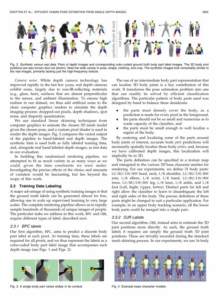
Fig. 2. Synthetic versus real data. Pairs of depth images and corresponding color-coded ground truth body part label images. The 3D body jointpositions are also known (but not shown). Note the wide variety in pose, shape, clothing, and crop. The synthetic images look remarkably similar tothe real images, primarily lacking just the high-frequency texture.

Fig. 3. A single body part varies widely in its context. Fig. 4. Example base character models.

joints: head, neck, L/R shoulder, L/R elbow, L/R wrist, L/R

hand, L/R knee, L/R ankle, and L/R foot. This selectionallows us to directly compare the BPC and OJR approacheson a common set of predicted joints.

3 METHOD

Our algorithms cast votes for the position of the body jointsby evaluating a sliding window decision forest at eachpixel. These votes are then aggregated to infer reliable 3Dbody joint position proposals. In this section, we describe:

1. the features we employ to extract discriminativeinformation from the image,

2. the structure of a random forest and how it combinesmultiple such features to achieve an accurate set ofvotes,

3. the different leaf node prediction models used forBPC and OJR,

4. how the pixel votes are aggregated into a set of jointposition predictions at test time, and

5. how the forests are learned.

3.1 Depth Image Features

We employ simple depth comparison features, inspired bythose in [44]. Individually these features provide only aweak discriminative signal, but combined in a decisionforest they prove sufficient to accurately disambiguatedifferent appearances and regions of the body. At a givenpixel u, the feature response is computed as

fðuj��Þ ¼ z uþ ��1

zðuÞ

� �� z uþ ��2

zðuÞ

� �; ð3Þ

where feature parameters �� ¼ ð��1; ��2Þ describe 2D pixeloffsets ��, and function zðuÞ looks up the depth at pixel u ¼ðu; vÞ> in a particular image. Each feature therefore per-forms two offset “depth probes” in the image and takestheir difference. The normalization of the offsets by 1

zðuÞensures that the feature response is depth invariant: At agiven point on the body, a fixed world space offset willresult whether the depth pixel is close or far from thecamera. The features are thus 3D translation invariant,modulo perspective effects. If an offset pixel u0 lies on thebackground or outside the bounds of the image, the depthprobe zðu0Þ is assigned a large positive constant value.

During training of the tree structure, offsets �� are sampledat random within a box of fixed size. We investigatesampling strategies in Section 3.5.1, and evaluate the effectof this maximum depth probe offset in Fig. 11c. We furtherset ��2 ¼ 0 with probability 1

2 . This means that roughly halfthe features evaluated are “unary” (look at only one offsetpixel) and half are “binary” (look at two offset pixels). Inpractice, the results appear to be fairly insensitive tothis parameter.

Fig. 5 illustrates two different features. The unary featurewith parameters ��1 looks upward: (3) will give a largepositive response for pixels u near the top of the body, but avalue close to zero for pixels u lower down the body. Bysimilar reasoning, the binary feature (��2) may be seeninstead to help find thin vertical structures such as the arm.

The design of these features was strongly motivated bytheir computational efficiency: No preprocessing is needed;each feature need only read at most three image pixels andperform at most five arithmetic operations. Further, thesefeatures can be straightforwardly implemented on the GPU.Given a larger computational budget, one could employpotentially more powerful features based on, for example,depth integrals over regions, curvature, or more complexlocal descriptors (e.g., [45]).

3.2 Randomized Forests

Randomized decision trees and forests [46], [47], [48], [49],[50] have proven fast and effective multiclass classifiers formany tasks [44], [51], [52], [50], and can be implementedefficiently on the GPU [12]. As illustrated in Fig. 6, a forest isan ensemble of T decision trees, each consisting of split andleaf nodes. We will use n to denote any node in the tree andl to denote a leaf node specifically. Each split node containsa “weak learner” represented by its parameters �� ¼ ð��; �Þ:The 2D offsets �� ¼ ð��1; ��2Þ used for feature evaluationabove, and a scalar threshold � . To make a prediction forpixel u in a particular image, one starts at the root andtraverses a path to a leaf by repeated evaluating the weaklearner function

hðu; ��nÞ ¼ fðu;��nÞ � �n½ �; ð4Þ

where ½�� is the 0-1 indicator. If hðu; ��nÞ evaluates to 0, thepath branches to the left child of n; otherwise it branches tothe right child. This repeats until a leaf node l is reached.We will use lðuÞ to indicate the particular leaf node reachedfor pixel u. The same algorithm is applied at each pixel foreach tree t, resulting in the set of leaf nodes reachedLðuÞ ¼ fltðuÞgTt¼1. More details can be found in [50], atutorial on decision forests.


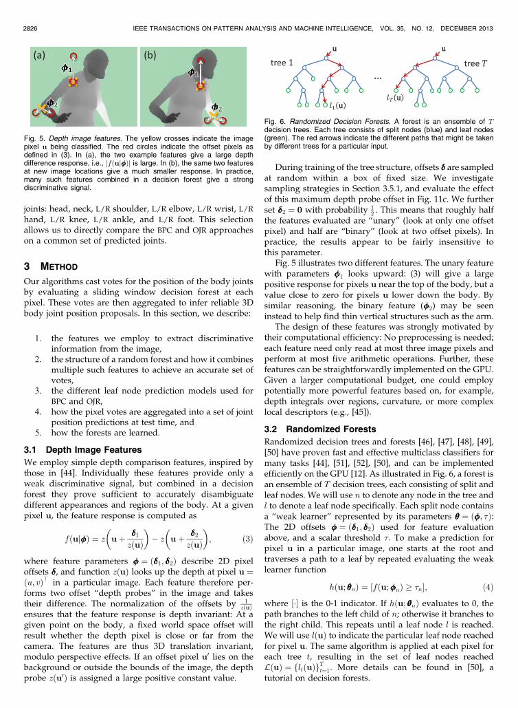
Fig. 5. Depth image features. The yellow crosses indicate the imagepixel u being classified. The red circles indicate the offset pixels asdefined in (3). In (a), the two example features give a large depthdifference response, i.e., jfðuj��Þj is large. In (b), the same two featuresat new image locations give a much smaller response. In practice,many such features combined in a decision forest give a strongdiscriminative signal.

Fig. 6. Randomized Decision Forests. A forest is an ensemble of Tdecision trees. Each tree consists of split nodes (blue) and leaf nodes(green). The red arrows indicate the different paths that might be takenby different trees for a particular input.

3.3 Leaf Node Prediction Models

At each leaf node l in each tree is stored a learned predictionmodel. In this work, we use two types of prediction model.For BPC, where a classification forest is used, the predictionmodel is a probability mass function plðcÞ over body parts c.For OJR, where a regression forest is used, the predictionmodel is instead a set of weighted relative votes Vlj for eachjoint j. In this section, we describe these two models, andshow how both algorithms can be viewed as casting a set ofweighted world space votes for the 3D positions of the eachjoint in the body. Section 3.4 will then show how these votesare aggregated in an efficient smoothing and clustering stepbased on mean shift to produce the final 3D body jointproposals.

3.3.1 Body Part Classification (BPC)

BPC predicts a body part label at each pixel as anintermediate step toward predicting joint positions. Theclassification forest approach achieves this by storing adistribution plðcÞ over the discrete body parts c at each leaf l.For a given input pixel u, the tree is descended to reach leafl ¼ lðuÞ and the distribution plðcÞ is retrieved. The distribu-tions are averaged together for all trees in the forest to givethe final classification as

pðcjuÞ ¼ 1

T

Xl2LðuÞ

plðcÞ: ð5Þ

One can visualize the most likely body part inferred ateach pixel as an image, and examples of this are given inFig. 10. One might consider smoothing this signal in theimage domain. For example, one might use probabilitiespðcjuÞ as the unary term in a conditional random fieldwith a pairwise smoothness prior [53]. However, since theper-pixel signal is already very strong and such smooth-ing would likely be expensive to compute, we do not usesuch a prior.

The image space predictions are next reprojected intoworld space. We denote the reprojection function asxðuÞ ¼ ðxðuÞ; yðuÞ; zðuÞÞ>. Conveniently, the known zðuÞfrom the calibrated depth camera allows us to compute xðuÞand yðuÞ trivially.

Next, we must decide how to map from surface bodyparts to interior body joints. In Section 2, we defined many,though not all, body part labels c to spatially align with thebody joints j, and conversely most joints j have a specificpart label c. We will thus use cðjÞ to denote the body partassociated with joint j.

Now, no matter how well aligned in the x and ydirections, the body parts inherently lie on the surface ofthe body. They thus cannot align in the z direction with theinterior body joint position we are after. (See Fig. 1.) Wetherefore use a learned per-joint vector ��j ¼ ð0; 0; �jÞ> thatpushes back the reprojected pixel surface positions into theworld to better align with the interior joint position:xjðuÞ ¼ xðuÞ þ ��j. This simple approach effectively as-sumes each joint is spherical, and works well and efficientlyin practice. As an indication, the mean across the differentjoints of the learned push-backs � is 0.04 m.

We finally create the set XBPCj of weighted world space

votes using Algorithm 1. These votes will be used in the

aggregation step below. As you can see, the position of eachvote is given by the pushed-back world space pixel positionxjðuÞ. The vote weight w is given by the probability massfor a particular body part multiplied by the squared pixeldepth. This depth-weighting compensates for observingfewer pixels when imaging a person standing further fromthe camera, and ensures the aggregation step is depthinvariant. In practice this gave a small but consistentimprovement in joint prediction accuracy.

Algorithm 1. Body part classification voting

1: initialize XBPCj ¼ ; for all joints j

2: for all foreground pixels u in the test image do

3: evaluate forest to reach leaf nodes LðuÞ4: evaluate distribution pðcjuÞ using (5)

5: compute 3D pixel position xðuÞ ¼ ðxðuÞ; yðuÞ; zðuÞÞ>6: for all joints j do

7: compute pushed-back position xjðuÞ8: lookup relevant body part cðjÞ9: compute weight w as pðc ¼ cðjÞjuÞ � z2ðuÞ

10: add vote ðxjðuÞ; wÞ to set XBPCj

11: return set of votes XBPCj for each joint j

Note that each pixel produces exactly one vote for eachbody joint, and these votes all share the same world spaceposition. In practice, many of the votes will have zeroprobability mass and can be ignored. This contrasts with theOJR prediction model, described next, where each pixel cancast several votes for each joint.

3.3.2 Offset Joint Regression

The OJR approach aims to predict the set of weighted votesdirectly, without going through an intermediate representa-tion. The forest used here is a regression forest [54], [50]since the leaves make continuous predictions. At each leafnode l we store a distribution over the relative 3D offset fromthe reprojected pixel coordinate xðuÞ to each body joint j ofinterest. Each pixel can thus potentially cast votes to alljoints in the body and, unlike BPC, these votes may differ inall world space coordinates and thus directly predictinterior rather than surface positions.

Ideally, one would like to make use of a distribution ofsuch offsets. Even for fairly deep trees, we have observedhighly multimodal empirical offset distributions at theleaves. Thus, for many nodes and joints approximating thedistribution over offsets as a Gaussian would be inap-propriate. One alternative, Hough forests [20], is torepresent the distribution as the set of all offsets seen attraining time. However, Hough forests trained on our largetraining sets would require vast amounts of memory and beprohibitively slow for a realtime system.

We therefore, in contrast to [36], [20], represent thedistribution using a small set of 3D relative vote vectors��ljk 2 IR3. The subscript l denotes the tree leaf node (asbefore), j denotes a body joint, and k 2 f1; . . . ; Kg denotes acluster index.1 We have found K ¼ 1 or 2 has given goodresults, and while the main reason for keeping K small isefficiency, we also empirically observed (Section 4.5.4) that


1. We use K to indicate the maximum number of relative votes allowed.In practice, we allow some leaf nodes to store fewer than K votes for somejoints.

increasing K beyond 1 gives only a very small increase in

accuracy. As described below, these relative votes are

obtained by clustering an unbiased sample of all offsets

seen at training time using mean shift (see Section 3.5.2).Unlike [37], a corresponding confidence weight wljk is

assigned to each vote, given by the size of its cluster, and

our experiments in Section 4.5.6 show these weights are

critical for high accuracy. We will refer below to the set ofrelative votes for joint j at node l as Vlj ¼ fð�ljk; wljkÞgKk¼1.

We detail the test-time voting approach for OJR inAlgorithm 2, whereby the set XOJR

j of absolute votes cast by

all pixels for each body joint j is collected. As with BPC, the

vote weights are multiplied by the squared depth to

compensate for differing surface areas of pixels. Optionally,

the set XOJRj can be subsampled by taking either the top

Nsub weighted votes or, instead, Nsub randomly sampled

votes. Our results show that this can dramatically improve

speed while maintaining high accuracy (Fig. 13c).

Algorithm 2. Offset joint regression voting

1: initialize XOJRj ¼ ; for all joints j

2: for all foreground pixels u in the test image do

3: evaluate forest to reach leaf nodes LðuÞ4: compute 3D pixel position xðuÞ ¼ ðxðuÞ; yðuÞ; zðuÞÞ>5: for all leaves l 2 LðuÞ do

6: for all joints j do

7: lookup weighted relative vote set Vlj8: for all ð�ljk; wljkÞ 2 Vlj do

9: compute absolute position x ¼ xðuÞ þ�ljk

10: compute weight w as wljk � z2ðuÞ11: add vote ðx; wÞ to set XOJR

j

12: subsample XOJRj to contain at most Nsub votes

13: return subsampled vote set XOJRj for each joint j

Compared to BPC, OJR more directly predicts joints that

lie behind the depth surface, and can cope with joints thatare occluded or outside the image frame. Fig. 7 illustrates

the voting process for OJR.

3.4 Aggregating Predictions

We have seen above how at test time both BPC and OJR can be

seen as casting a set of weighted votes in world space for

the location of the body joints. These votes must now be

aggregated to generate reliable proposals for the positionsof the 3D skeletal joints. Producing multiple proposals foreach joint allows us to capture the inherent uncertainty in thedata. These proposals are the final output of our algorithm.As we will see in our experiments, these proposals canaccurately localize the positions of body joints from a singleimage. Given a whole sequence, the proposals could also beused by a tracking algorithm to self-initialize and recoverfrom failure.

A simple option might be to accumulate the globalcentroid of the votes for each joint. However, the votes aretypically highly multimodal, and so such a global estimateis inappropriate. Instead we employ a local mode findingapproach based on mean shift [55].

We first define a Gaussian Parzen density estimator perjoint j as

pmj ðx0Þ /X

ðx;wÞ2Xmj

w � exp � x0 � x

bmj

��

20@

1A; ð6Þ

where x0 is a coordinate in 3D world space, m 2 fBPC;OJRg indicates the approach, and bmj is a learned per-jointbandwidth.

Mean shift is then used to find modes in this densityefficiently. The algorithm starts at a subset Xmj � Xmj of thevotes, and iteratively walks up the density by computingthe mean shift vector [55] until convergence. Votes thatconverge to the same 3D position within some tolerance aregrouped together, and each group forms a body jointproposal, the final output of our system. A confidenceweight is assigned to each proposal as the sum of theweights w of the votes in the corresponding group. For bothBPC and OJR this proved considerably more reliable thantaking the modal density estimate (i.e., the value pjðx0Þ). ForBPC the starting point subset XBPC

j is defined as all votes forwhich the original body part probability was above alearned probability threshold �cðjÞ. For OJR, all votes areused as starting points, i.e., XOJR

j ¼ XOJRj .

3.5 Training

Each tree in the decision forest is trained on a set of imagesrandomly synthesized using the method described inSection 2. Because we can synthesize training data cheaply,we use a different set of training images for each tree in the


Fig. 7. OJR voting at test time. Each pixel (black square) casts a 3D vote (orange line) for each joint. Mean shift is used to aggregate these votes andproduce a final set of 3D predictions for each joint. The highest confidence prediction for each joint is shown. Note accurate prediction of internalbody joints even when occluded.

forest. As described above, each image is fully labeled: ForBPC there is one body part label c per foreground pixel u,and for OJR there is instead one pose P ¼ ðp1; . . . ;pJÞ of 3Djoint position vectors pj per training image. For notationalsimplicity, we will assume that u uniquely encodes a 2Dpixel location in a particular image and thus can rangeacross all pixels in all training images. A random subset ofNex ¼ 2,000 example pixels from each image is used. Usinga subset of pixels reduces training time and ensures aroughly even contribution from each training image.

The following sections describe training the structure ofthe trees, the leaf node prediction models, and the hyper-parameters. Note that we can decouple the training of thetree structure from the training of the leaf predictors; moredetails are given below.

3.5.1 Tree Structure Training

To train the tree structure, and thereby the weak learnerparameters used at the split nodes, we use the standardgreedy decision tree training algorithm. At each node, a set Tof many candidate weak learner parameters �� 2 T issampled (these �� parameters are those used in (4)). Eachcandidate is then evaluated against an objective function I.Each sampled �� induces a partition of the set S ¼ fug of alltraining pixels that reached the node into left SLð��Þ andright SRð��Þ subsets according to the evaluation of the weaklearner function (4). The best �� is selected according to

��? ¼ argmin��2T

Xd2fL;Rg

jSdð��ÞjjSj IðSdð��ÞÞ; ð7Þ

which minimizes objective function I while balancing thesizes of the left and right partitions. We investigate bothclassification and regression objective functions, as de-scribed below. If the tree is not too deep, the algorithm thenrecurses on the example sets SLð��?Þ and SRð��?Þ for the leftand right child nodes, respectively.

Training the tree structure is by far the most expensivepart of the training process since many candidate para-meters must be tried at an exponentially growing number oftree nodes as the depth increases. To keep the training timespractical we employ a distributed implementation. At thehigh end of our experiments, training 3 trees to depth 20from 1 million images takes about a day on a 1,000 corecluster. (GPU-based implementations are also possible andmight be considerably cheaper.) The resulting trees eachhave roughly 500 K nodes, suggesting fairly balanced trees.

We next describe the two objective functions investigatedin this work.

Classification. The standard classification objective IclsðSÞminimizes the Shannon entropy of the distribution of theknown ground truth labels corresponding to the pixels in S.Entropy is computed as

IclsðSÞ ¼ �Xc

pðcjSÞ log pðcjSÞ; ð8Þ

where pðcjSÞ is the normalized histogram of the set of bodypart labels cðuÞ for all u 2 S.

Regression. Here, the objective is to partition theexamples to give nodes with minimal uncertainty in the

joint offset distributions at the leaves [56], [20]. In ourproblem, the offset distribution for a given tree node islikely to be highly multimodal (see examples in Fig. 9). Oneapproach might be to fit a Gaussian mixture model (GMM)to the offsets and use the negative log likelihood of theoffsets under this model as the objective. However, GMMfitting would need to be repeated at each node forthousands of candidate weak learners, making thisprohibitively expensive. Another possibility might be touse nonparametric entropy estimation [57], but again thiswould increase the cost of training considerably.

Following existing work [20], we instead employ themuch cheaper sum-of-squared-differences objective:

IregðSÞ ¼Xj

Xu2Sjk�u!j � ��jk

22; ð9Þ

where offset vector �u!j ¼ pj � xðuÞ, and

��j ¼1

jSjjXu2Sj

�u!j; ð10Þ

Sj ¼ u 2 S j k�u!jk2 < � �

: ð11Þ

Unlike [20], we introduce an offset vector length thresh-old to remove offsets that are large and thus likely to beoutliers (results in Section 4.5.1 highlight importance of ).While this model implicitly assumes a unimodal Gaussian,which we know to be unrealistic, for learning the treestructure this assumption is tractable and can still producesatisfactory results.

Discussion. Recall that the two objective functions aboveare used for training the tree structure. We are then at libertyto fit the leaf prediction models in a different fashion (seethe next section). Perhaps counterintuitively, we observedin our experiments that optimizing with the classificationobjective Icls works well for the OJR task. Training forclassification will result in image patches reaching the leafnodes that tend to have both similar appearances and localbody joint configurations. This means that for nearby joints,the leaf node offsets are likely to be small and tightlyclustered. The classification objective further avoids theassumption of the offset vectors being Gaussian distributed.

We did investigate further node splitting objectives,including various forms of mixing BPC and regression (asused in [20]), as well as variants such as separate regressionforests for each joint. However, none proved better thaneither the standard classification or regression objectivesdefined above.

Sampling ��. The mechanism for proposing T , the set ofcandidate weak learner parameters �� merits further discus-sion, especially as the search space of all possible �� is large.The simplest strategy is to sample jT j values of �� from auniform proposal distribution pð��Þ, defined here over somerange of offsets �� ¼ ð��1; ��2Þ and over some range ofthresholds � . If the forest is trained using this proposaldistribution, one finds that the empirical distribution pð��?Þ(computed over the chosen ��? across all nodes in the forest)ends up far from uniform.

This suggests an iterative strategy: Start from a uniformproposal distribution pð��Þ, train the forest, examine thedistribution pð��?Þ of the chosen ��?s, design an improved


nonuniform proposal distribution p0ð��Þ that approximatespð��?Þ, and repeat. The intuition is that if you show thetraining algorithm more features that are likely to be picked,it will not need to see so many to find a good one. To makethis procedure “safe,” the new proposal distribution p0ð��Þcan include a mixture with a uniform distribution with asmall mixture coefficient (e.g., 10 percent). In practice, weobserved a small but consistent improvement in accuracywhen iterating this process once (see Figs. 11e, 11f), thoughfurther iterations did not help. See Fig. 8 for an illustration.This idea is explored further in [58].

3.5.2 Leaf Node Prediction Models

Given the learned tree structure, we must now train theprediction models at the leaf nodes. It is possible to firsttrain the tree structure as described in the previous section,and then “retro-fit” the leaf predictors by passing all thetraining examples down the trained tree to find the set oftraining examples that reach each individual leaf node. Thisallows us to investigate the use of different tree structureobjectives for a given type of prediction model; see resultsbelow in Section 4.5.1.

For the BPC task, we simply take plðcÞ ¼ pðcjSÞ, thenormalized histogram of the set of body part labels cðuÞ forall pixels u 2 S that reached leaf node l.

For OJR, we must instead build the weighted relative votesets Vlj ¼ fð�ljk; wljkÞgKk¼1 for each leaf and joint. To do this,we employ a clustering step using mean shift, detailed inAlgorithm 3. This algorithm describes how each trainingpixel induces a relative offset to all ground truth jointpositions,2 and once aggregated across all training images,these are clustered using mean shift. To maintain practicaltraining times and keep memory consumption reasonable weuse reservoir sampling [59] to sample Nres offsets. Reservoirsampling is an algorithm that allows one to maintain a fixed-

size unbiased sample from a potentially infinite stream ofincoming samples; see [59] for more details. In our case, itallows us to uniformly sample Nres offsets at each node fromwhich to learn the prediction models without having to storethe much larger set of offsets being seen.

Algorithm 3. Learning relative votes1: // Collect relative offsets

2: initialize Rlj ¼ ; for all leaf nodes l and joints j

3: for all training pixels u 2 S do

4: descend tree to reach leaf node l ¼ lðuÞ5: compute 3D pixel position xðuÞ6: for all joints j do

7: lookup ground truth joint positions P ¼ fpjg8: compute relative offset �u!j ¼ pj � xðuÞ9: store �u!j in Rlj with reservoir sampling

10: // Cluster

11: for all leaf nodes l and joints j do

12: cluster offsets Rlj using mean shift

13: discard modes for which k�ljkk2 > threshold j14: take top K weighted modes as Vlj15: return relative votes Vlj for all nodes and joints

Mean shift mode detection is again used for clustering,

this time on the following density:

pljð�0Þ /X

�2Rlj

exp � �0 ��

b?

��

2 !

: ð12Þ

This is similar to (6), though now defined over relative offsets,without weighting, and using a learned bandwidth b?. Fig. 9visualizes a few examples sets Rlj that are clustered. Thepositions of the modes form the relative votes �ljk andthe numbers of offsets that reached each mode form thevote weights wljk. To prune out long range predictionswhich are unlikely to be reliable, only those relative votesthat fulfil a per joint distance threshold j are stored; thisthreshold could equivalently be applied at test time thoughit would waste memory in the tree. In Section 4.5.4, weshow that there is little or no benefit in storing more thanK ¼ 2 relative votes per leaf.

We discuss the effect of varying the reservoir capacity in

Section 4.5.7. In our unoptimized implementation, learning

these relative votes for 16 joints in 3 trees trained with 10 K

images took approximately 45 minutes on a single eight-core

machine. The vast majority of that time is spent traversing

the tree; the use of reservoir sampling ensures the time spent

running mean shift totals only about 2 minutes.

3.5.3 Learning the Hyperparameters

Some of the hyperparameters used in our methods are the

focus of our experiments below in Sections 4.4 and 4.5.

Others are optimized by grid search to maximize our mean

average precision (mAP) over a 5 K image validation set.

These parameters include the probability thresholds �c(the chosen values were between 0.05 and 0.3), the surface

push-backs �j (between 0.013 to 0.08 m), the test-time

aggregation bandwidths bmj (between 0.03 and 0.1 m), the

shared training-time bandwidth b? (0.05 m).


Fig. 8. Sampling strategies for ��. (a) A uniform proposal distribution isused to sample the 2D feature offsets �� (see (3)) during tree structuretraining. After training, a 2D histogram of the selected �� values across allsplit nodes in the forest is plotted. The resulting distribution is far fromuniform. (b) Building a mixture distribution to approximate these selectedoffsets, the tree structure training selects a similar distribution of offsets.However, as seen in Fig. 11e, Fig. 11f, this can have a substantialimpact on training efficiency.

2. Recall that for notational simplicity we are assuming u defines a pixelin a particular image; the ground truth joint positions P used will thereforecorrespond for each particular image.

4 EXPERIMENTS

In this section, we describe the experiments performed toevaluate our method on several challenging datasets. Webegin by describing the test datasets and error metricsbefore giving some qualitative results. Following that, weexamine in detail the effect of various hyper-parameters onBPC and then OJR. We finally compare the two methods,both to each other and to alternative approaches.

4.1 Test data

We use both synthetic and real depth images to evaluate ourapproach. For the synthetic test set (“MSRC-5000”), wesynthesize 5,000 test depth images, together with the groundtruth body part labels and body joint positions, using thepipeline described in Section 2. However, to ensure a fairand distinct test set, the original mocap poses used togenerate these test images are held out from the trainingdata. Our real test set consists of 8,808 frames of real depthimages over 15 different subjects, hand-labeled with densebody parts and seven upper body joint positions. We alsoevaluate on the real test depth data from [6].

As we will see, the results are highly correlated betweenthe synthetic and real data. Furthermore, our synthetic testset appears to be far “harder” than either of the real test setsdue to its extreme variability in pose and body shape. Aftersome initial experiments we thus focus our evaluation onthe harder synthetic test set.

In most of the experiments below, we limit the rotation ofthe user to �120 in both training and synthetic test datasince the user is facing the camera (0) in our mainentertainment scenario. However, we do also investigatethe full 360 degree scenario.

4.2 Error Metrics

We quantify accuracy using 1) a classification metric (forBPC only) and 2) a joint prediction metric (for both BPC andOJR). As the classification metric, we report the average per-class segmentation accuracy. This metric is computed as the

mean of the diagonal elements of the confusion matrixbetween the ground truth body part label and the mostlikely inferred label. This metric weights each body partequally despite their varying sizes.

As the joint prediction metric, we generate recall-precision curves as a function of the predicted confidencethreshold, as follows: All proposals below a given con-fidence threshold are first discarded; varying this thresholdgives rise to the full recall-precision curve. Then, the firstbody joint proposal within a threshold Dtp meters of theground truth position is taken as a true positive, while anyother proposals that are also within Dtp meters count asfalse positives. This penalizes multiple spurious detectionsnear the correct position which might slow a downstreamtracking algorithm. Any proposals outside Dtp meters alsocount as false positives. Any joint for which there is noproposal of sufficient confidence within Dtp is counted as afalse negative. However, we choose not to penalize jointsthat are invisible in the image as false negatives.

Given the full recall-precision curve, we finally quantifyaccuracy as average precision (the area under the curve) perjoint, or mAP over all joints. Note that, for example, a meansquared error (MSE) metric is inappropriate to evaluate ourapproach. Our algorithms aim to provide a strong signal toinitialize and reinitialize a subsequent tracking algorithm.As such, evaluating our approach on MSE would fail tomeasure joints for which there are zero or more than oneproposal, and would fail to measure how reliable the jointproposal confidence measures are. Our mAP metric effec-tively measures all proposals (not just the most confident):The only way to achieve a perfect score of 1 is to predictexactly one proposal for each joint that lies within Dtp of theground truth position. For most results below we set Dtp ¼0:1 m as the threshold, though we investigate the effect ofthis threshold below in Fig. 14c.

For BPC we observe a strong correlation of classificationand joint prediction accuracy (cf. the blue curves in Figs. 11aand 15b). This suggests the trends observed below for one


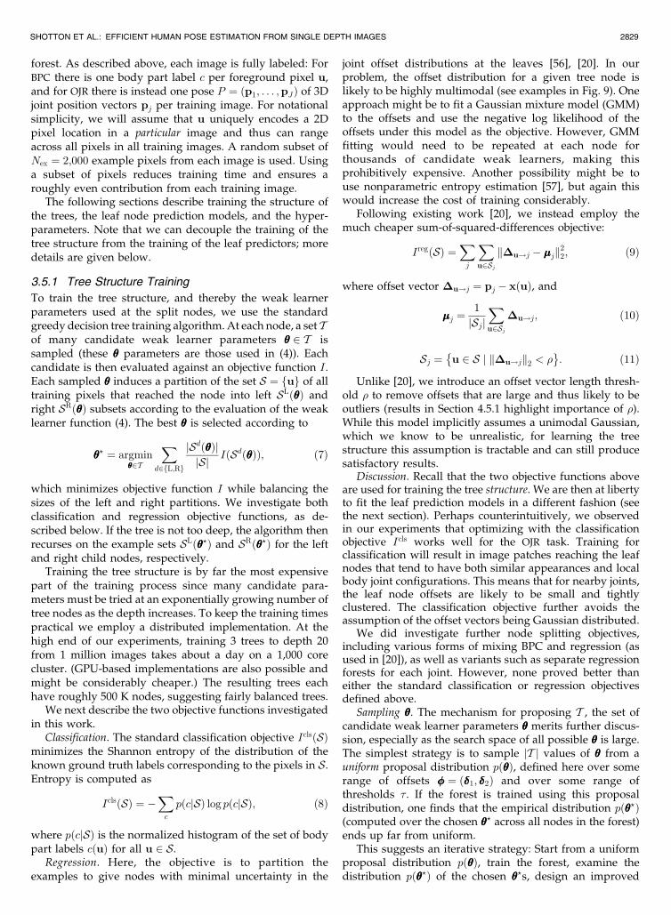
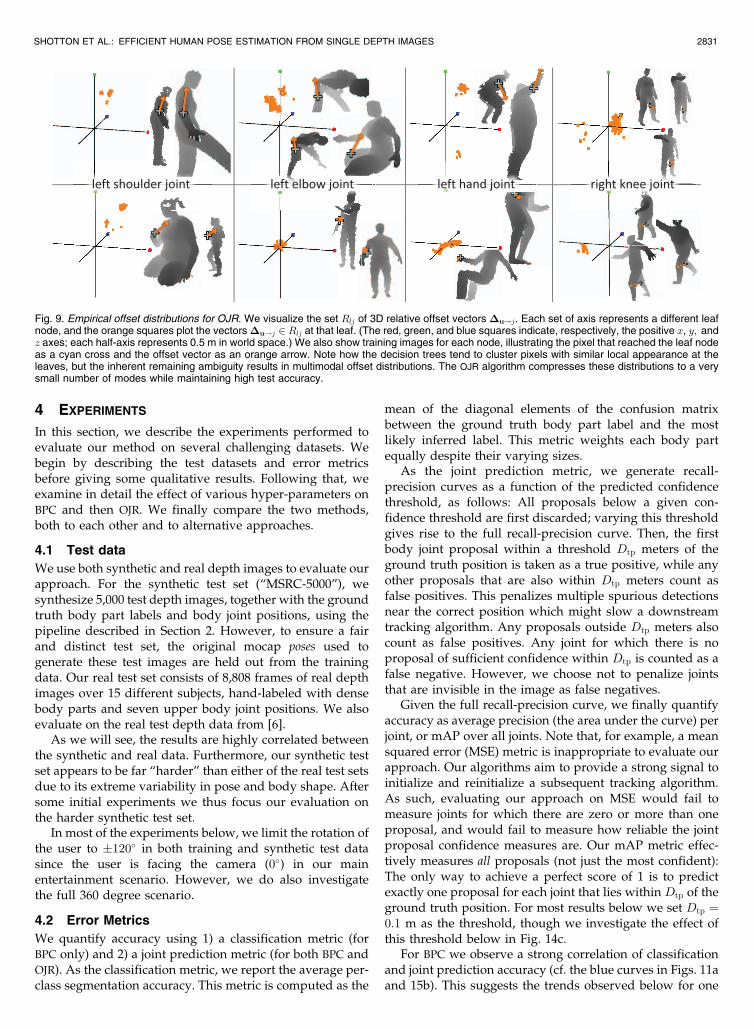
Fig. 9. Empirical offset distributions for OJR. We visualize the set Rlj of 3D relative offset vectors �u!j. Each set of axis represents a different leafnode, and the orange squares plot the vectors �u!j 2 Rlj at that leaf. (The red, green, and blue squares indicate, respectively, the positive x, y; andz axes; each half-axis represents 0.5 m in world space.) We also show training images for each node, illustrating the pixel that reached the leaf nodeas a cyan cross and the offset vector as an orange arrow. Note how the decision trees tend to cluster pixels with similar local appearance at theleaves, but the inherent remaining ambiguity results in multimodal offset distributions. The OJR algorithm compresses these distributions to a verysmall number of modes while maintaining high test accuracy.

also apply for the other. For brevity, we thus present results

below for only the more interesting combinations of

methods and metrics.

4.3 Qualitative results

Fig. 10 shows example inferences for both the BPC and OJR

algorithms. Note the high accuracy of both classification

and joint prediction, across large variations in body and

camera pose, depth in scene, cropping, and body size and

shape (e.g., small child versus heavy adult). Note that no

temporal or kinematic constraints (other than those im-

plicitly encoded in the training data) are used for any of our

results. When tested on video sequences (not shown), most

joints can be accurately predicted in most frames with

remarkably little jitter.A few failure modes are evident: 1) difficulty in

distinguishing subtle changes in depth such as the crossed

arms; 2) for BPC, the most likely inferred part may be

incorrect, although often there is still sufficient correct

probability mass in distribution pðcjuÞ that an accurate

proposal can still result during clustering; and 3) failure to

generalize well to poses not present in training. However, the

inferred confidence values can be used to gate bad proposals,

maintaining high precision at the expense of recall.In these and other results below, unless otherwise

specified, the following training parameters were used.

We trained 3 trees in the forest. Each was trained to depth

20, on 300 K images per tree, using Nex ¼ 2,000 training

example pixels per image. At each node we tested 2,000

candidate offset pairs �� and 50 candidate thresholds � per

offset pair, i.e., jT j ¼ 2,000 50. Below, unless specified, the

number of images used refers to the total number used by

the whole forest; each tree will be trained on a subset of

these images.

4.4 BPC Experiments

We now investigate the effect of several training parameters

on the BPC algorithm, using the classification accuracy

metric. The following sections refer to Fig. 11.

4.4.1 Number of Training Images

In Fig. 11a, we show how test accuracy increases approxi-

mately logarithmically with the number of randomly

generated training images, though it starts to tail off around

100 K images. This saturation could be for several reasons:

1) The model capacity of the tree has been reached; 2) the

error metric does not accurately capture the continued

improvement in this portion of the graph (e.g., the under-

lying probability distribution is improving but the MAP

label is constant); or 3) the training images are rendered

using a fixed set of only 100 K poses from motion capture

(though with randomly chosen body shapes, global rota-

tions, and translations). Given the following result, the first

of these possibilities is quite likely.

4.4.2 Depth of Trees

Fig. 11b shows how the depth of trees affects test accuracy

using either 15 K or 900 K images. Of all the training

parameters, depth appears to have the most significant effect

as it directly impacts the model capacity of the classifier.

Using only 15 K images we observe overfitting beginning

around depth 17, but the enlarged 900 K training set avoids

this. The high accuracy gradient at depth 20 suggests even

better results can be achieved by training still deeper trees at

a small extra runtime computational cost and a large extra

memory penalty.


Fig. 10. Example inferences on both synthetic and real test images. In each example, we see the input depth image, the inferred most likely bodypart labels (for BPC only), and the inferred body joint proposals shown as front, right, and top views overlaid on a depth point cloud. Only the mostconfident proposal for each joint above a fixed, shared threshold is shown, though the algorithms predict multiple proposals per joint. Both algorithmsachieve accurate prediction of body joints for varied body sizes, poses, and clothing. We show failure modes in the bottom rows of the two largerpanels. There is little qualitatively to tell between the two algorithms, though the middle row of the OJR results shows accurate prediction of evenoccluded joints (not possible with BPC), and further results in Section 4.6 compare quantitatively. Best viewed digitally at high zoom.

4.4.3 Maximum Probe Offset

The range of depth probe offsets �� allowed during traininghas a large effect on accuracy. We show this in Fig. 11c for5 K training images, where “maximum probe offset” meansthe maximum absolute value proposed for both x and ycoordinates of ��1 and ��2 in (3). The concentric boxes on theright show the five tested maximum offsets, calibrated for aleft shoulder pixel in that image (recall that the offsets scalewith the world depth of the pixel). The largest maximumoffset tested covers almost all the body. As the maximumprobe offset is increased, the classifier is able to use morespatial context to make its decisions. (Of course, because thesearch space of features is enlarged, one may need a largerset T of candidate features during training). Accuracyincreases with the maximum probe offset, though it levelsoff at around 129 pixel meters, perhaps because a largercontext makes overfitting more likely.

4.4.4 Number of Trees

We show in Fig. 11d test accuracy as the number of trees isincreased, using 5 K images for each depth 18 tree. Theimprovement starts to saturate around 4 or 5 trees, and isconsiderably less pronounced than when making the treesdeeper. The error bars give an indication of the remarkablysmall variability between trees. The qualitative resultsillustrate that more trees tend to reduce noise, though evena single tree can get the overall structure fairly well.

4.4.5 Number of features and thresholds

Figs. 11e, 11f shows the effect of the number of candidatefeatures �� and thresholds � evaluated during treetraining. Using the mixture proposal distributions for

sampling �� and � (see Section 3.5.1) allows for potentiallymuch higher training efficiency. Most of the gain occursup to 500 features and 20 thresholds per feature. On theeasier real test set the effects are less pronounced. Theseresults used 5 K images for each of 3 trees to depth 18.The slight peaks on the mixture proposal curves are likelydown to overfitting.

4.4.6 Discussion

The trends observed above on the synthetic and real testsets appear highly correlated. The real test set appearsconsistently “easier” than the synthetic test set, probablydue to the less varied poses present. For the remainingexperiments, we thus use the harder synthetic test set.

We now switch our attention to the joint predictionaccuracy metric. We have observed (for example, cf. theblue curves in Figs. 11a and 15b) a strong correlationbetween the classification and joint prediction metrics. Wetherefore expect that the trends observed above also applyto joint prediction.

4.5 Offset Joint Recognition (OJR) Experiments

The previous section investigated the effect of many of thesystem parameters for BPC. We now turn to the OJR

algorithm and perform a similar set of experiments. Theresults in this section all make use of the average precisionmetric on joint prediction accuracy (see Section 4.2).

4.5.1 Tree Structure Objectives

The task of predicting continuous joint locations from depthpixels is fundamentally a regression problem. Intuitively, wemight expect a regression-style objective function to producethe best trees for our approach. To investigate if this is


Fig. 11. Training parameters versus classification accuracy of the BPC algorithm. (a) Number of training images. (b) Depth of trees. (c) Maximumdepth probe offset. (d) Number of trees. (e), (f) Number of candidate features �� and thresholds � evaluated during training, for both real and synthetictest data, and using a uniform and mixture proposal distribution during tree structure training (see Section 3.5.1).

indeed the case, we evaluated several objective functions fortraining the structure of the decision trees, using foreststrained with 5 K images. The results, comparing averageprecision on all joints, are summarized in Fig. 12.

Surprisingly, for all joints except head, neck, andshoulders, trees trained using the classification objective Icls

(i.e., training the tree structure for BPC using (8), but thenretro-fitting the leaf prediction models for OJR; see Sec-tion 3.5.2) gave the highest accuracy. We believe theunimodal assumption implicit in the regression objective(9) may be causing this, and that classification of body parts isa reasonable proxy for a regression objective that correctlyaccounts for multimodality. A further observation fromFig. 12 is that the threshold parameter (used in (11) toremove outliers) does improve the regression objective, butnot enough to beat the classification objective.

Another possible problem with (9) could be the summa-tion over joints j. To investigate this, we experimented withtraining separate regression forests, each tasked withpredicting the location of just a single joint. A full forestwas trained with 5 K images for each of four representativejoints: head, l. elbow, l. wrist, and l. hand. With ¼ 1, theyachieved AP scores of 0.95, 0.564, 0.508, and 0.329,respectively (cf. the green bars in Fig. 12: 0.923, 0.403,0.359, and 0.198, respectively). As expected, due to greatermodel capacity (i.e., one forest for each joint versus oneforest shared for all joints), the per-joint forests producebetter results. However, these results are still considerablyworse than the regression forests trained with the classifica-tion objective.

Given these findings, the following experiments all usethe classification objective.

4.5.2 Tree Depth and Number of Trees

Fig. 13a shows that mAP rapidly improves as the tree depthincreases, though it starts to level off around depth 18. Aswith BPC, the tree depth is much more important than thenumber of trees in the forest: With just one tree, we obtain amAP of 0.730, with two trees 0.759, and with three trees 0.770.

4.5.3 Vote Length Threshold

We obtain our best results when using a separate votinglength threshold j for each joint (see Algorithm 3). Thesethresholds are optimized by grid search on a 5 K validationdataset, using a step size of 0.05 m in the range ½0:05; 0:60�m.In Fig. 13b, we compare accuracy obtained using a singlelearned threshold shared by all joints (the blue curve)against the mAP obtained with per-joint thresholds (thedashed red line). When using a shared threshold it appearscritical to include votes from pixels at least 10 cm away fromthe target joints. This is likely because the joints are typicallyover 10 cm away from the surface where the pixels lie.

We next investigate the effect of the metric used tooptimize these thresholds. Interestingly, the optimizedlength thresholds j turn out quite differently accordingto whether the failure to predict an occluded joint iscounted as a false negative or simply ignored. In Table 1, wesee that longer range votes are chosen to maximize mAPwhen the model is penalized for missing occluded joints. Insome cases, such as head, feet, and ankles, the difference is


TABLE 1Optimized Values for the Test-Time Vote Length Thresholds j

under Two Different Error Metrics

Fig. 12. Comparison of tree structure objectives used to train the OJRforest. In all cases, after the tree structure has been trained, the sameregression model is fit for each leaf node, as described in Section 3.5.2.

Fig. 13. Effect of various system parameters on the OJR algorithm. (a) mAP versus tree depth. (b) mAP versus a single, shared vote length thresholdfor all joints. (c) mAP versus fps. The blue curve is generated by varying Nsub, the number of votes retained before running mean shift at test time.

quite large. This makes sense: Occluded joints tend to befurther away from visible depth pixels than nonoccludedjoints, and predicting them will thus require longer rangevotes. This experiment used 30 K training images.

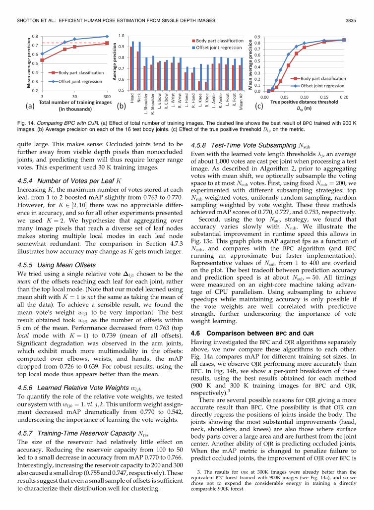
4.5.4 Number of Votes per Leaf K

Increasing K, the maximum number of votes stored at eachleaf, from 1 to 2 boosted mAP slightly from 0.763 to 0.770.However, for K 2 ½2; 10� there was no appreciable differ-ence in accuracy, and so for all other experiments presentedwe used K ¼ 2. We hypothesize that aggregating overmany image pixels that reach a diverse set of leaf nodesmakes storing multiple local modes in each leaf nodesomewhat redundant. The comparison in Section 4.7.3illustrates how accuracy may change as K gets much larger.

4.5.5 Using Mean Offsets

We tried using a single relative vote �lj1 chosen to be themean of the offsets reaching each leaf for each joint, ratherthan the top local mode. (Note that our model learned usingmean shift with K ¼ 1 is not the same as taking the mean ofall the data). To achieve a sensible result, we found themean vote’s weight wij1 to be very important. The bestresult obtained took wij1 as the number of offsets within5 cm of the mean. Performance decreased from 0.763 (toplocal mode with K ¼ 1) to 0.739 (mean of all offsets).Significant degradation was observed in the arm joints,which exhibit much more multimodality in the offsets:computed over elbows, wrists, and hands, the mAPdropped from 0.726 to 0.639. For robust results, using thetop local mode thus appears better than the mean.

4.5.6 Learned Relative Vote Weights wljkTo quantify the role of the relative vote weights, we testedour system withwljk ¼ 1; 8l; j; k. This uniform weight assign-ment decreased mAP dramatically from 0.770 to 0.542,underscoring the importance of learning the vote weights.

4.5.7 Training-Time Reservoir Capacity Nres

The size of the reservoir had relatively little effect onaccuracy. Reducing the reservoir capacity from 100 to 50led to a small decrease in accuracy from mAP 0.770 to 0.766.Interestingly, increasing the reservoir capacity to 200 and 300also caused a small drop (0.755 and 0.747, respectively). Theseresults suggest that even a small sample of offsets is sufficientto characterize their distribution well for clustering.

4.5.8 Test-Time Vote Subsampling Nsub

Even with the learned vote length thresholds j, an averageof about 1,000 votes are cast per joint when processing a testimage. As described in Algorithm 2, prior to aggregatingvotes with mean shift, we optionally subsample the votingspace to at most Nsub votes. First, using fixed Nsub ¼ 200, weexperimented with different subsampling strategies: topNsub weighted votes, uniformly random sampling, randomsampling weighted by vote weight. These three methodsachieved mAP scores of 0.770, 0.727, and 0.753, respectively.

Second, using the top Nsub strategy, we found thataccuracy varies slowly with Nsub. We illustrate thesubstantial improvement in runtime speed this allows inFig. 13c. This graph plots mAP against fps as a function ofNsub, and compares with the BPC algorithm (and BPC

running an approximate but faster implementation).Representative values of Nsub from 1 to 400 are overlaidon the plot. The best tradeoff between prediction accuracyand prediction speed is at about Nsub ¼ 50. All timingswere measured on an eight-core machine taking advan-tage of CPU parallelism. Using subsampling to achievespeedups while maintaining accuracy is only possible ifthe vote weights are well correlated with predictivestrength, further underscoring the importance of voteweight learning.

4.6 Comparison between BPC and OJR

Having investigated the BPC and OJR algorithms separatelyabove, we now compare these algorithms to each other.Fig. 14a compares mAP for different training set sizes. Inall cases, we observe OJR performing more accurately thanBPC. In Fig. 14b, we show a per-joint breakdown of theseresults, using the best results obtained for each method(900 K and 300 K training images for BPC and OJR,

respectively).3

There are several possible reasons for OJR giving a moreaccurate result than BPC. One possibility is that OJR candirectly regress the positions of joints inside the body. Thejoints showing the most substantial improvements (head,neck, shoulders, and knees) are also those where surfacebody parts cover a large area and are furthest from the jointcenter. Another ability of OJR is predicting occluded joints.When the mAP metric is changed to penalize failure topredict occluded joints, the improvement of OJR over BPC is


3. The results for OJR at 300K images were already better than theequivalent BPC forest trained with 900K images (see Fig. 14a), and so wechose not to expend the considerable energy in training a directlycomparable 900K forest.

Fig. 14. Comparing BPC with OJR. (a) Effect of total number of training images. The dashed line shows the best result of BPC trained with 900 Kimages. (b) Average precision on each of the 16 test body joints. (c) Effect of the true positive threshold Dtp on the metric.

even more apparent: 0.663 versus 0.560 (both methodstrained with 30 K images). Example inferences showinglocalization of occluded joints are presented in Fig. 10 (OJR

panel, middle row). As previously observed in Fig. 13c, theOJR algorithm can also make predictions faster than BPC.

4.6.1 True Positive Threshold

A value of Dtp ¼ 0:1 m is used as the true positive radius formost of the results presented here. We quantify the effect ofthis threshold on the mAP score in Fig. 14c. The OJR

algorithm maintains a considerably higher mAP score asthe radius shrinks in comparison to BPC.

4.6.2 Full Rotations

To evaluate the scenario of full 360 rotation of the user, wetrained BPC and OJR forests on images containing fullrotations, and tested on 5 K synthetic full rotation images.Despite the massive increase in left-right ambiguity, bothapproaches do remarkably well. Trained on 900 K images,the BPC forest achieved a mAP of 0.655, while, trained on300 K images, the OJR forest achieved a mAP of 0.711. Theseresults indicate that the forests can accurately learn thesubtle visual cues that distinguish front and back facingposes. The residual left-right ambiguity might be handledby a tracking algorithm that propagates multiple hypoth-eses through time.

4.6.3 Multiple People

Our approach can propose joint positions for multiplepeople in the image: Neither the forest evaluation at eachpixel nor the aggregation step are limited to a single person.The forest could be explicitly trained with images contain-ing multiple people, but in practice generalizes well withoutsuch explicit training. Preliminary results of this are givenin the supplementary video, which can be found online.

4.6.4 Silhouette Images

Although we focus on depth images in this paper, ourmethods can be applied without modification to 2Dsilhouette images. Silhouettes might readily be obtainedusing color segmentation or static background subtractionfrom RGB images. To prototype this scenario, we flattenedboth the training and test images to a fixed canonical depth,2 m, producing silhouettes in which the body size isunknown. To compute average precision for this 2Dprediction task, we modified the true positive radius to anabsolute pixel distance, Dtp ¼ 10 pixels. BPC achieves

0.465 mAP, and OJR achieves 0.596 mAP. Exampleinferences of OJR from silhouettes appear in the bottomright panel of Fig. 10, where the crosses show the groundtruth, and the circles show the inferred joint predictions.Note how the proposal confidences (shown as the circleradii) correlate well with the ambiguity in the signal. Themost probable reason for the significant drop in accuracy isdue to missing information. For example, whenever a handcrosses in front of the body, the silhouettes will likely notcontain enough information to reliably detect the hand.

4.7 Comparison to the State of the Art

In this final evaluation section, we compare our algorithmsto other methods.

4.7.1 Comparison to Ganapathi et al. [6]

Ganapathi et al. [6] kindly provided their test data andresults for direct comparison. Their algorithm uses sparsebody part proposals from [5] and further tracks the skeletonwith kinematic and temporal information. Their real datacomes from a time-of-flight depth camera with verydifferent noise characteristics to our structured light sensor.Without any changes to our training data or algorithm,Fig. 15a shows considerably improved joint predictionaverage precision for both BPC and OJR. Our algorithms alsorun at least 10 times faster, though we do of course requirethe large training corpus.

4.7.2 Whole Pose Nearest Neighbor Matching

Both of our methods attempt to find the body jointsindependently of each other. One alternative is to attemptto match a whole pose at once. Whole pose matching hasthe benefit of an extremely informative raw signal, butunfortunately has a search space that is exponential in thenumber of articulated joints. We compare our BPC

algorithm with two variants of whole pose matching inFig. 15b. The first, idealized, variant matches the groundtruth test skeleton to a set of training exemplar skeletons withoptimal rigid translational alignment in 3D world space. Ofcourse, in practice one has no access to the test skeleton.While this oracle is thus not an achievable algorithm, it doesgive us an upper bound on whole pose matching accuracy.As an example of a realizable system, the second variantuses chamfer matching [60] to compare the test image to thetraining exemplars. This is computed using depth edgesand 12 orientation bins. To make the chamfer task easier, wethrow out any cropped training or test images. We align


Fig. 15. Comparisons to the state of the art. (a) Comparison with [6]. Even without the kinematic and temporal constraints exploited by [6], both ourapproaches are able to more accurately localize body joints. (b) Comparison between BPC and nearest neighbor matching. Example chamfermatches shown right.

images using the 3D center of mass, and found that furtherlocal rigid translation only reduced accuracy.

Our BPC algorithm, recognizing in parts, generalizesbetter than even the idealized skeleton matching until about150K training images are reached. The speed of nearestneighbor chamfer matching is also drastically slower (2 fps)than our algorithm. While hierarchical matching [60] mightbe faster, one would still need a massive exemplar set toachieve comparable accuracy.

4.7.3 Comparison between OJR and Hough Forests [20]

We compare OJR and Hough forests [20], using an identicaltree structure for both. There are two main algorithmicdifferences. First, OJR clusters the offsets during training.This contrasts with Hough forests where all offset vectorsare stored. To compare, we retrain the leaf nodes of our OJR

forest, storing up to 400 offset votes for each joint, uniformlysampled (using all votes would have been prohibitive). Thesecond difference is that we use a continuous voting spaceat test time, while Hough forests instead discretize thevoting volume. Unfortunately, the inherent 3D nature ofour problem makes discrete voting much less attractivethan for 2D prediction. Our test data covers a large votingvolume of 4 4 5 m. To allow accurate localization weused a voxel resolution of 2 cm per side, resulting in avoting volume with 10 million bins. At test time, we smooththe voting volume using a Gaussian of fixed standarddeviation 1.3 cm.

Due to memory and runtime constraints we compare ontwo representative joints (an “easy” joint, head, and a“hard” joint, left hand) in Fig. 16. Interestingly, even withdiscrete voting, using two votes per leaf performs slightlybetter than voting with a large number of stored offsets.This is likely due to the clustering removing many outliersmaking the final density much peakier. The results alsoshow the clear improvement obtained by using theclassification objective to train the tree structure instead ofthe regression objective as used in [20]. (This reiterates thefindings from Fig. 12.)

Our implementation of the Hough voting ran at approxi-mately 0.5 fps for only 2 body joints, compared to around200 fps for OJR, which predicts all 16 joints. We experimentedwith a few voxel resolutions and smoothing kernel sizes,though the slow runtime speed prohibited selection of perjoint smoothing kernel widths by grid search.

5 CONCLUSIONS

We have presented two algorithms, BPC and OJR. The twoalgorithms have much in common. They both use decision

forests and simple depth-invariant image features. Bothmethods exploit a large, highly varied, synthetic trainingset, allowing us to train very deep trees. We have shownthat the forests can learn invariance to both pose and shapewhile avoiding overfitting. The BPC approach introduces aset of surface body parts that the forest tries to infer. Thesebody parts are aligned with the joints of interest so that anaccurate classification will localize the joints of the body.The OJR approach instead casts votes that try to directlypredict the positions of interior body joints. In bothmethods, mean shift is used to aggregate votes to producea final set of confidence-weighted 3D body joint proposals.

Our experiments have demonstrated that both algo-rithms can accurately predict the 3D locations of body jointsin super-real time from single depth or silhouette images.We have further shown state of the art accuracy and speedagainst several competing approaches. The body jointproposals might be used as an output in their own right,or used for initialization and reinitialization of a subsequenttracking and model fitting algorithm that exploits temporaland kinematic constraints.

Of our two approaches, which should you use? Thenumerical results show that OJR will give considerablyhigher accuracy than BPC. OJR also seems intuitively a“cleaner” solution: It does not need the intermediatedefinition of body parts, and the offsets vote directly forinterior joint positions. This also means that OJR is capableof predicting occluded joints, while BPC will instead give noproposals for an occluded joint. However, OJR provedconsiderably more complex: The obvious regression objec-tive does not work well, and many hyperparameters had tobe optimized against a validation set. A promising directionfor future work is to investigate alternative efficient tree-structure learning objectives that handle multimodal pro-blems effectively.

ACKNOWLEDGMENTS

The authors would like to thank the many skilled engineersat Microsoft who built the Kinect tracking system on top ofthis research. In particular: Robert Craig, Matt Bronder,Craig Peeper, Momin Al-Ghosien, Sam Mann, and RyanGeiss. They also thank John Winn, Duncan Robertson,Shahram Izadi, Ollie Williams, and Mihai Budiu for all theirhelp and discussions. Finally, thanks to Varun Ganapathiand Christian Plagemann for providing their test data. Thiswork was undertaken at Microsoft Research, Cambridge, incollaboration with Xbox.

REFERENCES

[1] D. Grest, J. Woetzel, and R. Koch, “Nonlinear Body PoseEstimation from Depth Images,” Proc. 27th DAGM Conf. PatternRecognition, 2005.

[2] S. Knoop, S. Vacek, and R. Dillmann, “Sensor Fusion for 3DHuman Body Tracking with an Articulated 3D Body Model,” Proc.IEEE Int’l Conf. Robotics and Automation, 2006.

[3] Y. Zhu and K. Fujimura, “Constrained Optimization for HumanPose Estimation from Depth Sequences,” Proc. Eighth Asian Conf.Computer Vision, 2007.

[4] M. Siddiqui and G. Medioni, “Human Pose Estimation from aSingle View Point, Real-Time Range Sensor,” Proc. IEEE Conf.Computer Vision and Pattern Recognition Workshops, 2010.

[5] C. Plagemann, V. Ganapathi, D. Koller, and S. Thrun, “Real-TimeIdentification and Localization of Body Parts from Depth Images,”Proc. IEEE Int’l Conf. Robotics and Automation, 2010.


Fig. 16. Comparison with Hough forest voting [20]. The Hough forest

regression objective performs poorly for articulated joint such as hands.

Vote compression and continuous voting improve accuracy slightly,

while running 3,200x faster (see text).

[6] V. Ganapathi, C. Plagemann, D. Koller, and S. Thrun, “Real TimeMotion Capture Using a Single Time-of-Flight Camera,” Proc.IEEE Conf. Computer Vision and Pattern Recognition, 2010.

[7] Microsoft Corp., Redmond, Wash., “Kinect.”[8] C. Bregler and J. Malik, “Tracking People with Twists and

Exponential Maps,” Proc. IEEE Conf. Computer Vision and PatternRecognition, 1998.

[9] L. Sigal, S. Bhatia, S. Roth, M. Black, and M. Isard, “TrackingLoose-Limbed People,” Proc. IEEE Conf. Computer Vision andPattern Recognition, 2004.

[10] R. Wang and J. Popovi�c, “Real-Time Hand-Tracking with a ColorGlove,” Proc. ACM Siggraph, 2009.

[11] M. Brubaker, D. Fleet, and A. Hertzmann, “Physics-Based PersonTracking Using the Anthropomorphic Walker,” Int’l J. ComputerVision, vol. 87, pp. 140-155, 2010.

[12] T. Sharp, “Implementing Decision Trees and Forests on a GPU,”Proc. European Conf. Computer Vision, 2008.

[13] R. Urtasun and T. Darrell, “Sparse Probabilistic Regression forActivity-Independent Human Pose Inference,” Proc. IEEE Conf.Computer Vision and Pattern Recognition, 2008.

[14] J. Shotton, A. Fitzgibbon, M. Cook, T. Sharp, M. Finocchio, R.Moore, A. Kipman, and A. Blake, “Real-Time Human PoseRecognition in Parts from a Single Depth Image,” Proc. IEEEConf. Computer Vision and Pattern Recognition, 2011.

[15] R. Fergus, P. Perona, and A. Zisserman, “Object Class Recognitionby Unsupervised Scale-Invariant Learning,” Proc. IEEE Conf.Computer Vision and Pattern Recognition, 2003.

[16] J. Winn and J. Shotton, “The Layout Consistent Random Field forRecognizing and Segmenting Partially Occluded Objects,” Proc.IEEE Conf. Computer Vision and Pattern Recognition, 2006.

[17] L. Bourdev and J. Malik, “Poselets: Body Part Detectors TrainedUsing 3D Human Pose Annotations,” Proc. IEEE Int’l Conf.Computer Vision, 2009.

[18] R. Girshick, J. Shotton, P. Kohli, A. Criminisi, and A. Fitzgibbon,“Efficient Regression of General-Activity Human Poses fromDepth Images,” Proc. IEEE Int’l Conf. Computer Vision, 2011.

[19] D. Comaniciu and P. Meer, “Mean Shift: A Robust Approachtoward Feature Space Analysis,” IEEE Trans. Pattern Analysis andMachine Intelligence, vol. 24, no. 5, pp. 603-619, May 2002.

[20] J. Gall and V. Lempitsky, “Class-Specific Hough Forests for ObjectDetection,” Proc. IEEE Conf. Computer Vision and Pattern Recogni-tion, 2009.

[21] T. Moeslund, A. Hilton, and V. Kruger, “A Survey of Advances inVision-Based Human Motion Capture and Analysis,” ComputerVision and Image Understanding, vol. 104, pp. 90-126, 2006.

[22] R. Poppe, “Vision-Based Human Motion Analysis: An Overview,”Computer Vision and Image Understanding, vol. 108, pp. 4-18, 2007.

[23] M. Fischler and R. Elschlager, “The Representation and Matchingof Pictorial Structures,” IEEE Trans. Computers, vol. 22, no. 1,pp. 67-92, Jan. 1973.

[24] P. Felzenszwalb and D. Huttenlocher, “Pictorial Structures forObject Recognition,” Int’l J. Computer Vision, vol. 61, no. 1, pp. 55-79, Jan. 2005.

[25] S. Ioffe and D. Forsyth, “Probabilistic Methods for FindingPeople,” Int’l J. Computer Vision, vol. 43, no. 1, pp. 45-68, 2001.

[26] D. Ramanan and D. Forsyth, “Finding and Tracking People fromthe Bottom Up,” Proc. IEEE Conf. Computer Vision and PatternRecognition, 2003.

[27] Z. Tu, “Auto-Context and Its Application to High-Level VisionTasks,” Proc. IEEE Conf. Computer Vision and Pattern Recognition,2008.

[28] D. Anguelov, B. Taskar, V. Chatalbashev, D. Koller, D. Gupta, andA. Ng, “Discriminative Learning of Markov Random Fields forSegmentation of 3D Scan Data,” Proc. IEEE Conf. Computer Visionand Pattern Recognition, 2005.

[29] E. Kalogerakis, A. Hertzmann, and K. Singh, “Learning 3D MeshSegmentation and Labeling,” ACM Trans. Graphics, vol. 29, no. 3,article 102, 2010.

[30] A. Agarwal and B. Triggs, “3D Human Pose from Silhouettes byRelevance Vector Regression,” Proc. IEEE Conf. Computer Visionand Pattern Recognition, 2004.

[31] A. Kanaujia, C. Sminchisescu, and D. Metaxas, “Semi-SupervisedHierarchical Models for 3D Human Pose Reconstruction,” Proc.IEEE Conf. Computer Vision and Pattern Recognition, 2007.

[32] R. Navaratnam, A.W. Fitzgibbon, and R. Cipolla, “The JointManifold Model for Semi-Supervised Multi-Valued Regression,”Proc. IEEE Int’l Conf. Computer Vision, 2007.

[33] G. Mori and J. Malik, “Estimating Human Body ConfigurationsUsing Shape Context Matching,” Proc. IEEE Int’l Conf. ComputerVision, 2003.

[34] G. Shakhnarovich, P. Viola, and T. Darrell, “Fast Pose Estimationwith Parameter Sensitive Hashing,” Proc. IEEE Int’l Conf. ComputerVision, 2003.

[35] G. Rogez, J. Rihan, S. Ramalingam, C. Orrite, and P. Torr,“Randomized Trees for Human Pose Detection,” Proc. IEEE Conf.Computer Vision and Pattern Recognition, 2008.

[36] B. Leibe, A. Leonardis, and B. Schiele, “Robust Object Detectionwith Interleaved Categorization and Segmentation,” Int’lJ. Computer Vision, vol. 77, nos. 1-3, pp. 259-289, 2008.

[37] J. Muller and M. Arens, “Human Pose Estimation with ImplicitShape Models,” Proc. First ACM Int’l Workshop Analysis andRetrieval of Tracked Events and Motion in Imagery Streams, 2010.

[38] R. Okada and S. Soatto, “Relevant Feature Selection for HumanPose Estimation and Localization in Cluttered Images,” Proc. 10thEuropean Conf. Computer Vision, 2008.

[39] H. Ning, W. Xu, Y. Gong, and T.S. Huang, “DiscriminativeLearning of Visual Words for 3D Human Pose Estimation,” Proc.IEEE Conf. Computer Vision and Pattern Recognition, 2008.

[40] H. Sidenbladh, M. Black, and L. Sigal, “Implicit ProbabilisticModels of Human Motion for Synthesis and Tracking,” Proc.Seventh European Conf. Computer Vision, 2002.

[41] T. Gonzalez, “Clustering to Minimize the Maximum InterclusterDistance,” Theoretical Computer Science, vol. 38, pp. 293-306, 1985.

[42] CMU Mocap Database, http://mocap.cs.cmu.edu/, 2013.[43] Autodesk MotionBuilder.[44] V. Lepetit, P. Lagger, and P. Fua, “Randomized Trees for Real-

Time Keypoint Recognition,” Proc. IEEE Conf. Computer Vision andPattern Recognition, pp. 2:775-781, 2005.

[45] S. Belongie, J. Malik, and J. Puzicha, “Shape Matching and ObjectRecognition Using Shape Contexts,” IEEE Trans. Pattern Analysisand Machine Intelligence, vol. 24, no. 4, pp. 509-522, Apr. 2002.

[46] B. Shepherd, “An Appraisal of a Decision Tree Approach to ImageClassification,” Proc. Eight Int’l Joint Conf. Artificial Intelligence,1983.

[47] J.R. Quinlan, “Induction of Decision Trees,” Machine Learning,vol. 1, pp. 81-106, 1986.

[48] Y. Amit and D. Geman, “Shape Quantization and Recognitionwith Randomized Trees,” Neural Computation, vol. 9, no. 7,pp. 1545-1588, 1997.

[49] L. Breiman, “Random Forests,” Machine Learning, vol. 45, no. 1,pp. 5-32, 2001.

[50] A. Criminisi, J. Shotton, and E. Konukoglu, “Decision Forests: AUnified Framework,” Foundations and Trends in Computer Graphicsand Vision, vol. 7, pp. 81-227, 2012.

[51] F. Moosmann, B. Triggs, and F. Jurie, “Fast Discriminative VisualCodebooks Using Randomized Clustering Forests,” Proc. Advancesin Neural Information Processing Systems, vol. 19, pp. 985-992, 2006.

[52] J. Shotton, M. Johnson, and R. Cipolla, “Semantic Texton Forestsfor Image Categorization and Segmentation,” Proc. IEEE Conf.Computer Vision and Pattern Recognition, 2008.

[53] J. Shotton, J. Winn, C. Rother, and A. Criminisi, “TextonBoost:Joint Appearance, Shape and Context Modeling for Multi-ClassObject Recognition and Segmentation,” Proc. European Conf.Computer Vision, 2006.

[54] A. Criminisi, J. Shotton, D. Robertson, and E. Konukoglu,“Regression Forests for Efficient Anatomy Detection and Locali-zation in CT Studies,” Proc. Int’l MICCAI Conf. Medical ComputerVision, 2010.

[55] D. Comaniciu and P. Meer, “Mean Shift: A Robust Approachtoward Feature Space Analysis,” IEEE Trans. Pattern Analysis andMachine Intelligence, vol. 24, no. 5, pp. 603-619, May 2002.

[56] T. Hastie, R. Tibshirani, J. Friedman, and J. Franklin, “TheElements of Statistical Learning: Data Mining, Inference andPrediction,” The Math. Intelligencer, vol. 27, no. 2, pp. 83-85, 2005.

[57] S. Nowozin, “Improved Information Gain Estimates for DecisionTree Induction,” Proc. Int’l Conf. Machine Learning, 2012.

[58] A. Montillo, J. Shotton, J. Winn, J. Iglesias, D. Metaxas, and A.Criminisi, “Entangled Decision Forests and Their Application forSemantic Segmentation of CT Images,” Proc. 22nd Int’l Conf.Information Processing in Medical Imaging, 2011.

[59] J.S. Vitter, “Random Sampling with a Reservoir,” ACM Trans.Math. Software, vol. 11, no. 1, pp. 37-57, 1985.


[60] D. Gavrila, “Entangled Decision Forests and Their Application forSemantic Segmentation of CT Images,” Proc. European Conf.Computer Vision, June 2000.

Jamie Shotton received the BA degree incomputer science and the PhD degree incomputer vision from the University ofCambridge, and worked as a postdoctoralToshiba fellow at Toshiba’s Corporate Re-search and Development Center in Japan. Heis a senior researcher in the Machine Learningand Perception Group at Microsoft ResearchCambridge, where he has been since 2008.His recent work has focused on human pose

estimation for Microsoft’s Kinect camera. This work was awarded theBest Paper Award at CVPR 2011 and the Royal Academy ofEngineering’s MacRobert Award 2011. His broader on-going researchincludes gesture and action recognition, object recognition, medicalimaging, and machine learning. He is a senior member of the IEEE.

Ross Girshick received the BS degree incomputer science from Brandeis University, theMS degree in computer science from theUniversity of Chicago, and the PhD degree incomputer science from the University ofChicago, where he was advised by PedroFelzenszwalb. While completing his PhDstudies, he led winning entries in the PASCALVOC object detection challenge. He also in-terned as a researcher at Microsoft Research

Cambridge. He is a postdoctoral fellow working with Jitendra Malik at theUniversity of California, Berkeley. His primary research interests includedeveloping representations and machine learning techniques for objectrecognition.

Andrew Fitzgibbon studied at University Col-lege Cork, at Heriot-Watt University, and re-ceived the PhD degree from EdinburghUniversity in 1997. Until June 2005, he held aRoyal Society University Research Fellowship atOxford University’s Department of EngineeringScience. He is a principal researcher at Micro-soft Research, Cambridge. His research inter-ests include the intersection of computer visionand computer graphics, with occasional excur-

sions into machine learning and neuroscience. His recent papers havebeen on models of nonrigid motion, human 3D perception, large-scaleimage search, and nonlinear optimization. He has coauthored “bestpapers” at ICCV, CVPR, ISMAR, and BMVC, and the software hewrote won an Engineering Emmy Award in 2002 for significantcontributions to the creation of complex visual effects. He is a seniormember of the IEEE.

Toby Sharp received the BSc degree in mathe-matics from the University of York. He is aprincipal research software development engi-neer in the Machine Learning and PerceptionGroup at Microsoft Research, Cambridge, wherehe has worked since 2005. He has transferredseveral research projects into Microsoft technol-ogies and products, and has contributed com-puter vision components to Microsoft’s Kinect,Office, and LifeCam software. His other work

includes computer graphics, image editing, and GPU programming.Prior to joining Microsoft, he developed consumer photo and videoediting software for Serif in the United Kingdom. In 2010, he received theExcellence in Design Award from RSNA for real-time virtual colono-scopy software. In 2011, he and colleagues received the Best Paperprize at CVPR and the Royal Academy of Engineering MacRobertAward for the machine learning contribution to Kinect’s body tracking.He is a senior member of the IEEE.

Mat Cook received the BSc degree in physicsfrom Imperial College, London. He is a devel-oper at Microsoft Research. He specializes ingraphics and synthetic ground truth generation.He played a key role on the team that builtKinect’s body part recognition algorithm. Thiswon the Best Paper Award at CVPR 2011 andthe Royal Academy of Engineering’s MacRobertAward in 2011.

Mark Finocchio received the BS degree inelectrical engineering and the MS degree incomputer science, both from New Mexico StateUniversity. He is a principal software engineer inthe Xbox Incubation Group at Microsoft, wherehe has been since 1997. He is a recipient of theMicrosoft Technical Recognition Award for Out-standing Technical Achievement for his work onreal-time human pose estimation for Kinect.

Richard Moore received the graduation degreefrom the University of California, San Diego, andthe master’s degree from Pepperdine University,in management science and business adminis-tration, respectively. He is a director of researchand development at ST-Ericsson. Prior to ST-Ericsson, he was in the Paris labs of RolandMoreno, the inventor of the smart card, and invarious start-ups in communications and ima-ging, before joining Microsoft’s Xbox incubation

team responsible for Kinect. He is a member of the IEEE.

Pushmeet Kohli is a research scientist in theMachine Learning and Perception Group atMicrosoft Research Cambridge, and an associ-ate of the Psychometric Centre, University ofCambridge. His PhD thesis written at OxfordBrookes University was the winner of the BritishMachine Vision Association’s Sullivan DoctoralThesis Award, and a runner-up for the BritishComputer Society’s Distinguished DissertationAward. His research revolves around intelligent

systems and computational sciences, with a particular emphasis onalgorithms and models for scene understanding and human poseestimation. His papers have appeared in SIGGRAPH, NIPS, ICCV,AAAI, CVPR, TPAMI, IJCV, CVIU, ICML, AISTATS, AAMAS, UAI,ECCV, and ICVGIP and have won Best Paper Awards in ECCV 2010,ISMAR 2011, and ICVGIP 2006, 2010.

Antonio Criminisi received the electronicsengineering degree from the University ofPalermo and the doctor of philosophy degreein computer vision at the University of Oxford inJuly 1996 and December 1999, respectively. Hejoined Microsoft Research Cambridge as avisiting researcher in 2000. In 2001, he movedto the Interactive Visual Media Group in Red-mond, Washington, as a postdoctoral research-er. In 2002, he moved back to Cambridge to join

the Vision Group as a researcher. In September 2011, he became asenior researcher and now leads the medical image analysis team. Hisresearch interests include medical image analysis, object recognition,image and video analysis and editing, teleconferencing, 3D reconstruc-tion with application to virtual reality, forensic science, and history of art.His thesis “Accurate Visual Metrology from Single and MultipleUncalibrated Images” won the British Computer Society DistinguishedDissertation Award 2000. He has won a number of best paper prizes intop computer vision conferences.


Alex Kipman received the graduation degree insoftware engineering from the Rochester Insti-tute of Technology. He is the general managerof incubation for the interactive entertainmentbusiness at Microsoft. An innovator and avisionary, he hand-selected and led the teamthat developed Kinect. He is the primaryinventor of Kinect and is named on 60 patentsdirectly related to Kinect. Among other honors,he was named one of TIME Magazine’s 2011

100 People of the Year.

Andrew Blake is a Microsoft DistinguishedScientist and has been the laboratory directorof Microsoft Research Cambridge, UnitedKingdom, since 2010. Prior to joining Microsoft,he trained in mathematics and electrical engi-neering in Cambridge, and studied for a doc-torate in artificial intelligence in Edinburgh. Hehas been a pioneer in the development of thetheory and algorithms that allow computers tobehave as seeing machines. He has published

several books, has twice won the prize of the European Conference onComputer Vision, and was awarded the IEEE David Marr Prize in 2001.In 2006, the Royal Academy of Engineering awarded him its SilverMedal, and in 2007 the Institution of Engineering and Technologypresented him with the Mountbatten Medal. He was elected a fellow ofthe Royal Academy of Engineering in 1998, of the IEEE in 2008, and ofthe Royal Society in 2005. In 2010, he was elected to the council of theRoyal Society. In 2011, he and colleagues received the Royal Academyof Engineering MacRobert Award for their machine learning contributionto Microsoft Kinect. He is a fellow of the IEEE.

. For more information on this or any other computing topic,please visit our Digital Library at www.computer.org/publications/dlib.


IEEE TRANSACTIONS ON PATTERN ANALYSIS AND MACHINE ... · PDF fileEfficient Human Pose...

Documents

Transcript of IEEE TRANSACTIONS ON PATTERN ANALYSIS AND MACHINE ... · PDF fileEfficient Human Pose...