IEEE TRANSACTIONS ON PATTERN ANALYSIS AND …cns.bu.edu/~gsc/Articles/Scarloff_Shape_FEM.pdfIEEE...

IEEE TRANSACTIONS ON PATTERN ANALYSIS AND MACHINE INTELLIGENCE, VOL. 13, NO. 7, JULY 1991 715

Closed-Form Solutions for Physically Based Shape Mode ling and Recognition

I

Alex Pentland and StaI Sclaroff, Member, IEEE

Abstract-We present a closed-form, physically based solution for recovering a 3-D solid model from collections of 3-D surface measurements. Given a sufficient number of independent measurements, the solution is overconstrained and unique except for rotational symmetries. We then present a physically based object- recognition method that allows simple, closed-form comparisons of recovered 3-D solid models. The performance of these methods is evaluated using both synthetic range data with various signal- to-noise ratios and using laser rangefinder data.

Index Terms-deformable models, finite element method, model analysis, modal-based vision, object recognition, physically based modeling, shape representation, 3-D shape recovery.

I. INTRODUCTION

V ISION research has a long tradition of trying to go from collections of low-level measurements to higher

level “part” descriptions such as generalized cylinders [l]- [3], deformed superquadrics [4]-[7], or geons [S], and then of attempting to perform object recognition. The general idea is to use part-level modeling primitives to bridge the gap between image features (points, edges, or corners) and the symbolic, parts-and-connections descriptions useful for recognition and reasoning [9].

Recently, several researchers have successfully addressed the first of these problems-that of recovering part descript ions-using deformable models. There have been two classes of such deformable models: those based on parametric solid model ing primitives, such as our own work using superquadr ics [4], and those based on mesh-l ike surface models, such as employed by Terzopoulos et al. [lo]. In the case of parametric modeling, fitting has been performed using the model ing primitive’s “inside-outside” function [5]-[7], [ll], whereas in the mesh surface models, a physical- motivated energy function has been employed [lo].

The description of shape by use of orthogonal parameters has the advantage that it can produce a unique, compact description that is well suited for recognit ion and database search but has the d isadvantage that it may not have enough degrees of f reedom to account for fine surface details. The deformable mesh approach, in contrast, is very good for describing shape details but produces descriptions that are

Manuscript received September 20, 1990; revised January 9, 1991. This work was supported in part by the National Science Foundation under Grant IRI-8719920, by the Rome Air Development Center (RADC) of the Air Force System Command, and the Defense Advanced Research Projects Agency (DARPA) under contract F30602-89-C-0022.

The authors are with the Vision and Modeling Group, The Media Labora- tory, Massachusetts Institute of Technology, Cambridge, MA 02139.

IEEE Log Number 9100890.

More importantly, however, we have been able to obtain and develop a formulation whose degrees of f reedom are orthogonal, and thus decoupled, by posing the dynamic equat ions in terms of the FEM equat ions’ eigenvectors. These eigenvectors are known as the object’s free vibration or deformation modes, and together, they form a f requency-ordered orthonormal basis set analogous to the Fourier transform.

By decoupl ing the degrees of f reedom, we achieve substan- tial

.

.

idvantages: The fitting problem has a simple, efficient, closed-form solution. The model’s intrinsic complexity can be adjusted to match the number of degrees of f reedom in the data measurements so that the solution can always be made overconstrained.

. When overconstrained, the solution is unique, except for rotational symmetries and degenerate conditions. Thus, the solution is well suited for recognit ion and database tasks.

neither unique nor compact and, consequent ly, cannot be used for recognit ion or database search without additional layers of processing. Both of these approaches share the d isadvantage that they are relatively slow, requiring dozens of iterations in the case of the parametric formulation, and up to hundreds of iterations in the case of the physically based mesh formulation.

W e have addressed these problems by adopt ing an approach based on the finite element method (FEM) and parametric solid model ing using implicit functions. This approach provides both the convenience of parametric model ing and the expressiveness of the physically based mesh formulation and, in addition, can provide great accuracy at physical simulation. Thus, it is possible to use the models we recover from range data to accurately simulate particular materials and situations for purposes of prediction, visualization, planning, and so forth WI, [=I.

The plan of this paper is to first review our representation. W e will then demonstrate its use in obtaining closed-form solutions to the shape recovery problem. Finally, we will demonstrate how closed-form compar ison of different object models can be used to obtain accurate object recognit ion from range data.

II. BACKGROUND: THE REPRESENTATION

Our representat ion descr ibes objects using the force-and- process metaphor of model ing clay: Shape is thought of as the result of pushing, pinching, and pulling on a lump of elastic material such as clay [4], [ll], [12]. The mathematical

0162~8828/91/0700-0715$01.00 0 1991 IEEE

716 IEEE TRANSACTIONS ON PAlTERN ANALYSIS AND MACHINE INTELLIGENCE, VOL. 13, NO. 7, JULY 1991

formulation is based on the FEM, which is the standard engineer ing technique for simulating the dynamic behavior of an object.

The notion of employing physical constraints in shape model ing has been suggested by many authors [4], [13], [14]; however, the seminal paper by Terzopoulos et al. [lo], who obtained 3-D models by fitting simulated rubbery sheets and tubes, has focused attention on model ing methods that draw on the mathematics used for simulating the dynamics of real objects. One motivation for using such physically based representat ions is that vision is often concerned with estimating changes in position, orientation, and shape, quantit ies that models such as the FEM accurately describe. Another motivation is that by allowing the user to specify forces that are a function of sensor measurements, the intrinsic dynamic behavior of techniques such as the FEM can be used to solve fitting, interpolation, or cor respondence problems.

In the FEM, interpolation functions that allow cont inuous material properties, such as mass and stiffness, to be integrated across the region of interest, are developed. Note that this is quite different from the finite difference schemes commonly used in computer vision, as is explained in Appendix A, al though the resulting equat ions are quite similar. One major difference between the FEM and the finite difference schemes is that the FEM provides an analytic characterization of the surface between nodes or pixels, whereas finite difference methods do not. All of the results presented in this paper will be applicable to both the finite difference and finite element formulations.

Having formulated the appropriate FEM integrals, they are then combined into a description in terms of discrete nodal points. Energy functionals are then formulated in terms of nodal displacements U, and the resulting set of s imultaneous equat ions is iterated to solve for the nodal displacements as a function of impinging loads R

Mij+CiJ+KU=R (1)

where U is a 3n x 1 vector of the (AX, Ay, AZ) displacements of the n nodal points relative to the object’s center of mass, M, C, and K are 3n by 3n matrices describing the mass, damping, and material stiffness between each point within the body, and R is a 3n x 1 vector describing the x, y, and z components of the forces acting on the nodes.

Equat ion (1) is known as the governing equat ion in the FEM and may be interpreted as assigning a certain mass to each nodal point and a certain material stiffness between nodal points, with damping being accounted for by dashpots at tached between the nodal points. Inertial and centrifugal effects are accounted for by adding appropriate off-diagonal terms to the mass matrix.

When a constant load is appl ied to a body, it will, over time, come to an equilibrium condit ion descr ibed by

KU=R. (2)

This equat ion is known as the equilibrium governing equation. The solution of the equilibrium equat ion for the nodal displacements U (and thus of the analytic surface interpolation

functions) is the most common objective of finite element analyses. In shape modeling, sensor measurements are used to define virtual forces that deform the object to fit the data points. The equilibrium displacements U constitute the recovered shape.

The most obvious drawback of all the physically based methods are their large computat ional expense. These methods reqUire roughly 3nmk operat ions per time step, where 3n is the order of the stiffness matrix and mk is its half bandwidth.’ Normally, 3n time steps are required to obtain an equilibrium solution. For a full 3-D model, where typically mk M 3n/2, the computat ional cost scales as 0 ( n3). Because of this poor scaling behavior, equat ions are sometimes discarded in order to obtain sparse banded matrices (for example, in [lo], those equat ions corresponding to internal nodes were discarded). In this case the computat ional expense is reduced to “only” o(n2mk).

A related drawback in vision applications is that the number of description parameters is often greater than the number of sensor measurements, necessitat ing the use of heuristics such as symmetry and smoothness. This also results in nonunique and unstable descriptions, with the consequence that it is normally difficult to determine whether or not two models are equivalent.

Perhaps the most important problem with using physically based models for vision, however, is that all of the degrees of f reedom are coupled together. Thus, closed-form solutions are impossible, and solutions to the inverse problems encountered in vision are very difficult.

A. Modal Analysis

Thus, there is a need for a method that transforms (1) into a form that is not only less costly but also allows closed-form solution. Since the number of operat ions is proport ional to the half bandwidth mk of the stiffness matrix, a reduct ion in mk will greatly reduce the cost of step-by-step solution. Moreover, if we can actually diagonal ize the system of equations, then the degrees of f reedom will become uncoupled, and we will be able to find closed-form solutions. To accomplish this goal, we utilize an FEM technique known as ModalAnalysis; in the remainder of this section, we develop this method along the lines of Bathe [15].

To diagonal ize the system of equations, a linear transformation of the nodal point displacements U can be used

U=PcJ (3)

where P is a square orthogonal transformation matrix and 0 is a vector of general ized displacements. Substituting (3) into (1) and premultipling by PT yields

- 2 MU+CU+tiU=ti (4)

where

ti = PTMP; c = PWP; l!i = P*KP; ii = PTR. (5)

‘See Bathe [15] Appendix A.2.2 for complete discussion on bandwidth of a stiffness matrix.

PENTLAND AND SCLAROFF: CLOSED-FORM SOLUTIONS 717

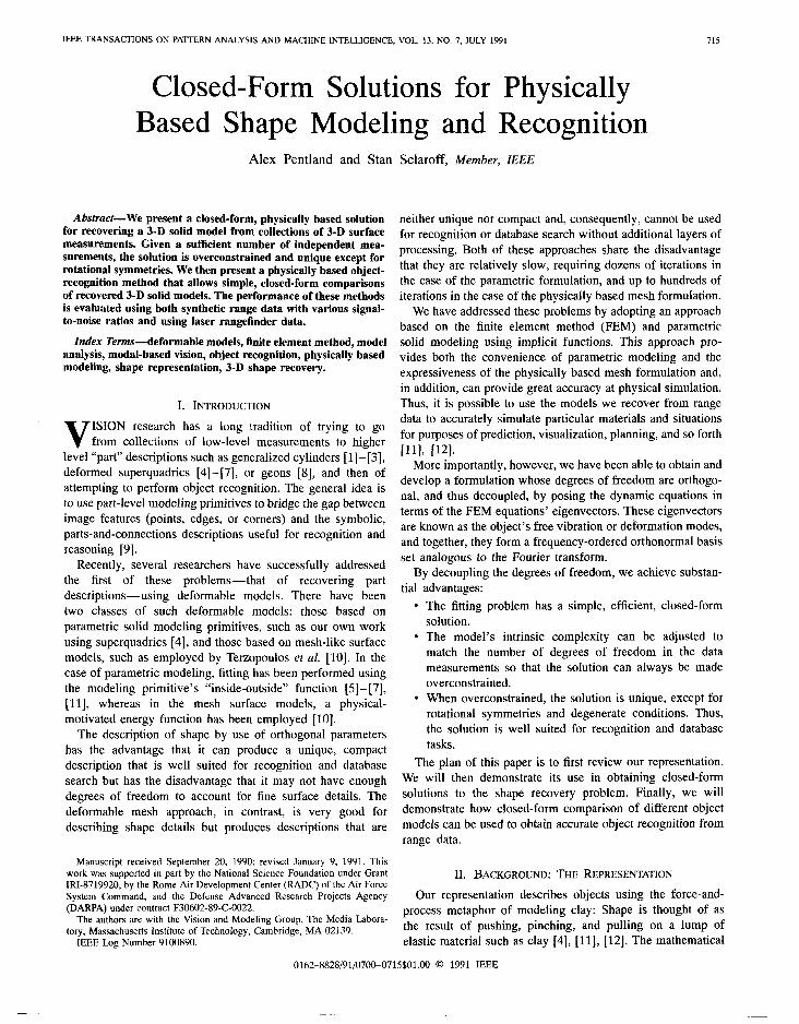
Fig. 1. Several of the lowest frequency vibrations modes of a cylinder. English labels are for descriptive purposes only.

W ith this transformation of basis set, a new system of stiffness, mass, and damping matrices that has a smaller bandwidth than the original system can be obtained.

1) Use of Free Vibration Modes: The optimal transformation matrix P is der ived from the free vibration modes of the equilibrium equation. Beginning with the governing equation, an eigenvalue problem can be derived

which will determine an optimal transformation basis set. The eigenvalue problem in (6) yields 3n eigensolut ions

where all the eigenvectors are M orthonormalized. Hence

i=j i#.i (7)

and

The eigenvector 4r is called the ith mode’s shape vector and wi is the corresponding f requency of vibration. Each eigenvector 4i consists of the (2, y, .z) displacements for each node, that is, the 3j - 2, 3j - 1, and 3j elements are the Z, y, and z displacements for node j, 1 5 j 5 n.

The lowest f requency modes are always the rigid-body modes of translation and rotation. The eigenvector corresponding to x-axis translation, for instance, has ones for each node’s x-axis displacement element, with all other elements being zero. Rotational motion is l inearized, so that nodes on the opposite sides of the body have opposite directions of displacement.

The next-lowest f requency nodes are smooth, whole-body deformations that leave the center of mass and rotation fixed. That is, the (z, y, Z) displacements of the nodes are a low-order function of the node’s position, and the nodal displacements balance out to zero net translational and rotational motion. Compact bodies (simple solids whose dimensions are within the same order of magnitude) normally have low-order modes that are similar to those shown in Fig. 1. Bodies with very dissimilar dimensions, or which have holes, etc., can have very complex low-frequency modes.

Using these modes we can define a transformation matrix @ ‘, which has for its columns the eigenvectors &, and a diagonal matrix n2, with the eigenvalues w” on its diagonal

Using (lo), (6) can now be written as

KG = 52’9M

and since the eigenvectors are M-orthonormal:

(11)

@K@ = 52’ +TM* = I. (12)

From the above formulations it becomes apparent that matrix Cp is the optimal transformation matrix P for systems in which damping effects are negligible.

To also diagonal ize the damping matrix C with the same transform, C must be restricted to a special form. The normal assumption is that the damping matrix is constructed by using the Caughey series [15]

P-l

C = M 1 ak [M-IK]! k=O

(13)

Restriction to this form is equivalent to the assumption that damping, which descr ibes the overall energy dissipation during the system response, is proport ional to system response. For p < 2, (13) reduces to Ruyleigh dumping (C = aaM + arK), and C is diagonal ized by +. Rayleigh damping is the most common type of damping used in finite element analysis [15].

Under the assumption of Rayleigh damping the general governing equation, given by (4), is reduced to

2’ U + et + a20 = @R(t) (14)

where C = a01 + ala’, or equivalently to 3n independent and individual equat ions of the form

ii&) + c&(t) + w&(t) = Pi(t) (15)

where & are modal damping parameters and ?i(t) = +TR(t) for i = 1,2,3,. . . , 3n. Therefore the matrix 9 is the optimal transformation for both damped and undamped systems, given that Rayleigh damping is assumed.

In summary, then, it has been shown that the general finite element governing equat ion is decoupled when using a transformation matrix P whose columns are the free vibration mode shapes of the FEM system [II], [12], [15]. These decoupled equat ions may then be integrated numerically (see [12]) or solved in c losed form for any future time t by use of a Duhamel integral (see [ll]).

718 IEEE TRANSACTIONS ON PATTERN ANALYSIS AND MACHINE INTELLIGENCE, VOL. 13, NO. 7, JULY 1991

III. RECOVERING 3-D PART MODELS FROM 3-D SENSOR MEASUREMENTS

Let us assume that we are given m three-dimensional sensor measurements (in the global coordinate system) that originate from the surface of a single object

X” = [~~,Y~,Z~,...,~~,Y~,Z~lT. (16) Following Terzopoulos et al., we then attach virtual springs between these sensor measurement points and particular nodes on our deformable model. This def ines an equilibrium equation whose solution U is the desired fit to the sensor data. Consequent ly, for m nodes with corresponding sensor measurements, we can calculate the virtual loads R exerted on the undeformed object while fitting it to the sensor measurements. For node Ic these loads are simply

LT3k > T3k+l, T3k+2] T = [z:, yr, .$lT - [Zkr !-/k, ZklT (17)

where

x = [~l,Y1,Zl,...r~nrYn,z~lT (18) are the nodal coordinates of the undeformed object in the object’s coordinate frame. When sensor measurements do not correspond exactly with existing nodes, the loads can be distributed to surrounding nodes using the interpolation functions H used to define the finite element model, as descr ibed in Appendix A. An inexpensive method of accomplishing this is d iscussed in Appendix B.

Thus to fit a deformable solid to the measured data we solve the following equilibrium equation:

KU=R (19)

where the loads R are as above, the material stiffness matrix K is as descr ibed above and in Appendix A, and the equilibrium displacements U are to be solved for. The solution to the fitting problem is simply

U = K-‘R. (20)

The difficulty in calculating this solution is the large dimensionality of K, so that iterative solution techniques are normally employed.

However, a closed-form solution is available simply by convert ing this equat ion to the modal coordinate system.2

This is accompl ished by substituting U = 90 and premul- tiplying by aT, so that the equilibrium equat ion becomes

9TK+U = (PTR c-21)

or equivalently

Rij=fi (22)

where R = (PTR and R = +TK+ is a diagonal matrix (see (12)). Again, note that the calculation of @ needs to be performed only once as a precomputat ion, and then stored for all future applications. Further, it is normally not desirable to use all of the eigenvectors (as explained in the next section),

*The solution is closed form in the sense that it is noniterative, requiring only multiplying a data term by a precomputed matrix of eigenvectors.

so that the ip matrix remains of manageab le size even when using large numbers of nodes. In our implementation G is normally a 30 x 3n matrix, where n is the number of nodes.

The solution to the fitting problem, therefore, is obtained by inverting the diagonal matrix K

fi = R-l&. (23)

Note, however, that as this formulation is posed in the object’s coordinate system the rigid body modes have zero eigenvalues, and must therefore be solved for separately by setting GZL; = Y;, 1 5 i 5 6. The complete solution may be written in the original nodal coordinate system, as follows:

U=Q(K+IG)19TR (24)

where 16 is a matrix whose first six diagonal elements are ones, and remaining elements are zero.3

The major difficulty in calculating this solution occurs when there are fewer degrees of f reedom in sensor measurements than in the nodal posit ions-as is normally the case in computer vision applications. Previous researchers have suggested adopt ing heuristics such as smoothness and symmetry to obtain a wel l -behaved solution; however, in many cases the observed objects are neither smooth nor symmetric, and so an alternative method is desirable.

W e believe that a better, and certainly simpler, method is to discard some of the high-frequency modes, so that the number of degrees of f reedom in U is equal to or less than the number of degrees of f reedom in the sensor measurements. To accomplish this, one simply row and column reduces I?, and column reduces @ so that their rank is less than or equal to the number of available sensor measurement degrees of f reedom. The motivation for this strategy is that:

l when there are fewer degrees of f reedom in the sensor measurements than in the model, the high-frequency modes cannot in any sense be accurate, as there is insufficient data to constrain them. Their value primarily reflects the smoothness heuristic employed.

l While the high-frequency modes will not contain information, they are the dominant factor determining the cost of the solution, as they are both numerous and require the use of very small time steps [12].

l In any case, high-frequency modes typically have very little energy, and even less effect on the overall object shape. This is because (for a given excitatory energy) the displacement ampli tude for each mode is inversely proport ional to the square of the mode’s resonance frequency, and because damping is proport ional to a mode’s frequency. The consequence of these combined effects is that high-frequency modes general ly have very little amplitude. Indeed, in structural analysis of airframes and buildings it is s tandard practice to discard such high- f requency modes.

‘Inclusion of the matrix 1~ into (24) may also be interpreted as adding an external force that constrains the solution to have no residual translational or rotational stresses.


Perhaps the most interesting consequence of discarding some of the high-frequency modes, however, is that it allows (24) to provide a generically overconstrained estimate of object shape. Note that discarding high-frequency modes is not equivalent to a smoothness assumption, as sharp corners, creases, etc., can still be obtained. What we cannot do with a reduced-basis modal representat ion is place many creases or spikes close together.

A. Determining Spring Attachment Points

Attaching a virtual spring between a data measurement and a deformable object implicitly specifies a cor respondence between some of the model’s nodes and the sensor measurements. In most situations this cor respondence is not given, and so must be determined in parallel with the equilibrium solution. In our exper ience this at tachment problem is the most problematic aspect of the physically based model ing paradigm. This is not surprising, however, as the attachment problem is similar to the cor respondence problems found in many other vision applications.

Our approach to the spring attachment problem is similar to that adopted by other researchers [6], [lo]. Given a segmentat ion of the data into objects or “blobs,” the first step is to define an ellipsoidal coordinate system by examinat ion of the data’s moments of inertia. Data points are then projected onto this ellipsoid in order to determine the spring attachment points. W e will descr ibe only the simplest form of this method, one that does not adjust for uneven sampling of the data, as the general approach is well known.

The center of the object is taken to be its center of gravity, except that because we see only the front-facing surface of the object we must employ a symmetry assumption to determine the z coordinate. After the center of gravity is found, we then determine the object’s orientation, which is assumed to be the same as its axes of inertia. The inertia matrix for sample range data consists of the moments of inertia and the cross products of inertia

I= J (y2 + z”) dm -Jxydm

-Jxydm J(x2+z2)dm -Jxzdm -Syzdm J(x2+y2)dm 1.

(25)

The eigenvectors of this matrix are the axes of inertia for the data points, and thus correspond roughly with the axes of inertia for the object. The eigenvector with the smallest e igenvalue corresponds to the most e longated axis of the body, and the eigenvector with the largest e igenvalue corresponds to the shortest axis. Finally, to obtain estimates of the z, y, and z dimensions, we inverse transform the sample points (using the rotation matrix built from the eigenvectors obtained in the previous step), measure the x, y, and z range, and finally double the size estimate along the view direction.

These estimates of position, orientation, and size define an elliptical coordinate system. To establish the cor respondence between sensor measurements and the nodes of the unde-

formed model, the sensor measurements are converted to this coordinate system and the latitude w and longitude Q of each data point is calculated. W e can find w by observing

G= cos v sin w T = tanw 2 cos r) cos w

where (s,c, 2) is the coordinate of the sensor measurement in the elliptical coordinate system. Thus w = atan@/%). Given w, 77 is determined by either 77 = atan((Z cos w)/?) or q = atan( (.Z sin w)/g) depending on whether Z or 6 is larger.

By using the FEM interpolation functions H, the virtual load generated by each data point is then distributed to the nodes whose posit ions surround the data point’s latitude and longitude. W e have found, however, that when there are enough nodes, most data points project near a node; consequent ly, it is sufficiently accurate to distribute these virtual loads to the three surrounding nodal points using simple bilinear interpolation. This is d iscussed further in Appendix B.

For simple objects (e.g., cubes, bananas, cylinders) our ex- perimental results show that this method of establishing spring attachment points yields accurate, unique object descriptions. It should be noted, however, that because 9 linearizes object rotation it is important that the elliptical coordinate system establ ished by the moment method be sufficiently close to the object’s true coordinate system. W e have found that as long as our initial estimate of orientation is within f15’ we can still achieve a stable, accurate estimate of shape.

For complex objects, however, the spring attachment problem is sufficiently nonl inear that we have found that it nec- essary to establish attachment posit ions iteratively. W e accomplish this by first fitting a solid model as above, and then use that der ived model to more accurately determine the spring attachment locations. In our experiments we have found that two or three iterations of this procedure are normally sufficient to produce a good solution to both the spring attachment and the fitting problems.

B. Examples of Recovering 3-D Models

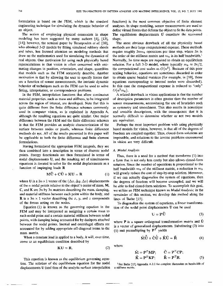
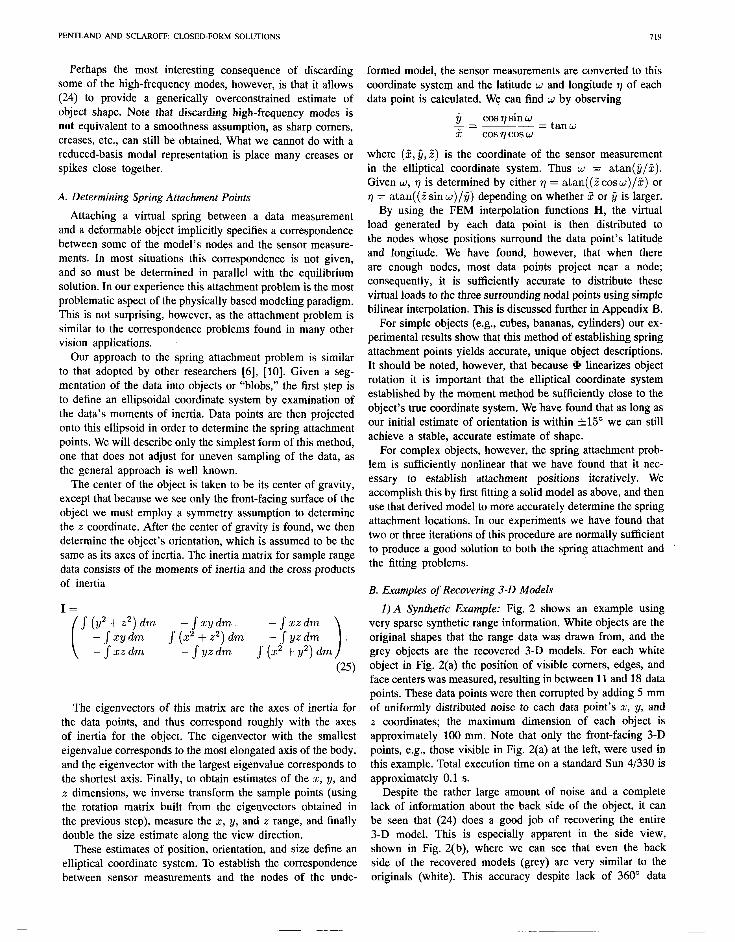
1) A Synthetic Example: Fig. 2 shows an example using very sparse synthetic range information. White objects are the original shapes that the range data was drawn from, and the grey objects are the recovered 3-D models. For each white object in Fig. 2(a) the position of visible corners, edges, and face centers was measured, resulting in between 11 and 18 data points. These data points were then corrupted by adding 5 mm of uniformly distributed noise to each data point’s x, y, and z coordinates; the maximum dimension of each object is approximately 100 mm. Note that only the front-facing 3-D points, e.g., those visible in Fig. 2(a) at the left, were used in this example. Total execut ion time on a standard Sun 4/330 is approximately 0.1 s.

Despite the rather large amount of noise and a complete lack of information about the back side of the object, it can be seen that (24) does a good job of recovering the entire 3-D model. This is especially apparent in the side view, shown in Fig. 2(b), where we can see that even the back side of the recovered models (grey) are very similar to the originals (white). This accuracy despite lack of 360” data

720 IEEE TRANSACTIONS ON PATTERN ANALYSIS AND MACHINE INTELLIGENCE, VOL. 13, NO. 7, JULY lYY1

Fig. 2. Front (a) and side (b) views of fitting a rectangular box, cylinder, banana, etc., using sparse 3-D point data with 5% noise. The original models are shown in white, and the recovered models are shown in darker grey. Given the positions of some of the object’s visible surface points (as shown in (a)), we can recover the full 3-D model as is shown in the side view (b).

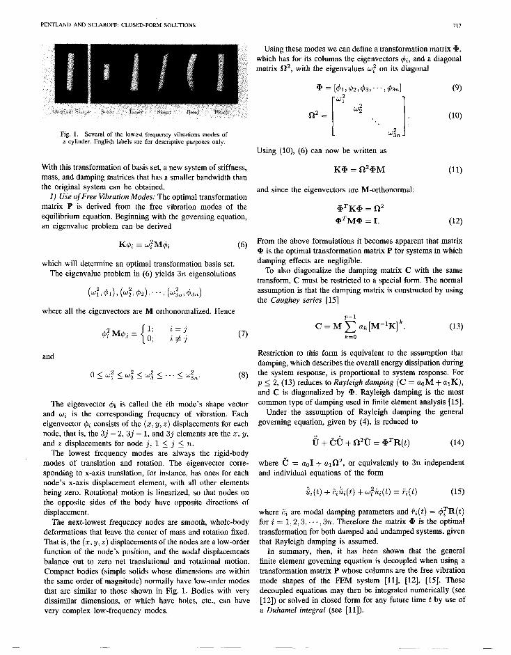
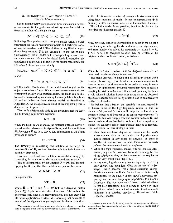
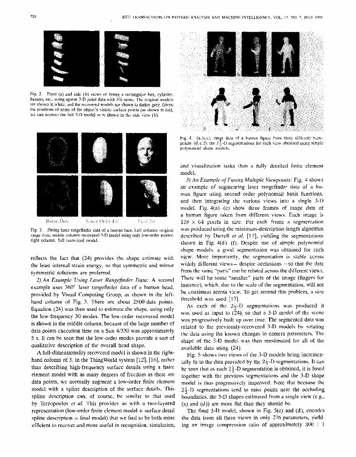
Fig. 4. (a,b,c): range data of a human figure from three different viewpoints. (d, e, f): the 2 3 -D segmentat ions for each view obtained using simple polynomial shape models.

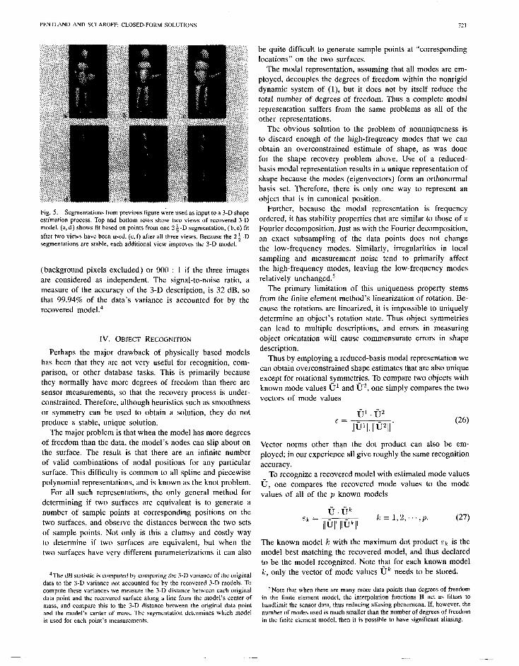
Fig. 3. Fitting laser rangefinder data of a human face. Left column: original range data; middle column: recovered 3-D model using only low-order modes: right column: full recovered model.

reflects the fact that (24) provides the shape estimate with the least internal strain energy, so that symmetric and mirror symmetric solutions are preferred.

2) An Example Using Laser Rangefinder Data: A second example uses 360” laser rangef inder data of a human head, provided by Visual Comput ing Group, as shown in the left- hand column of Fig. 3. There are about 2500 data points. Equat ion (24) was then used to estimate the shape, using only the low-frequency 30 modes. The low-order recovered model is shown in the middle column; because of the large number of data points execut ion time on a Sun 41330 was approximately 5 s. It can be seen that the low-order modes provide a sort of qualitative description of the overall head shape.

A full-dimensionality recovered model is shown in the right- hand column of 3. In the ThingWorld system [12], [16], rather than describing high-frequency surface details using a finite element model with as many degrees of f reedom as there are data points, we normally augment a low-order finite element model with a spline description of the surface details. This spline description can, of course, be similar to that used by Terzopoulos et al. This provides us with a two-layered representat ion (low-order finite element model + surface detail spline description = final model) that we find to be both more efficient to recover and more useful in recognition, simulation,

and visualization tasks than a fully detailed finite element model.

3) An Example of Fusing Multiple Viewpoints: Fig. 4 shows an example of segment ing laser rangef inder data of a human figure using second order polynomial basis functions, and then integrating the various views into a single 3-D model. Fig. 4(a)-(c) show three frames of range data of a human figure taken from different views. Each image is 128 x 64 pixels in size. For each frame a segmentat ion was produced using the minimum-description-length algorithm descr ibed by Darrell et al. [17], yielding the segmentat ions shown in Fig. 4(d)-(f). Despite use of simple polynomial shape models, a good segmentat ion was obtained for each view. More importantly, the segmentat ion is stable across widely different views-despite occlusions-so that the data from the same “parts” can be related across the different views. There will be some “smaller” parts of the image (fingers for instance), which, due to the scale of the segmentat ion, will not be consistent across view. To get a round this problem, a size threshold was used [17].

As each of the 2;-D segmentat ions was produced it was used as input to (24) so that a 3-D model of the scene was progressively built up over time. The segmented data was related to the previously-recovered 3-D models by rotating the data using the known changes in camera parameters. The shape of the 3-D model was then reestimated for all of the available data using (24).

Fig. 5 shows two views of the 3-D models being incremen- tally fit to the data provided by the 2$-D segmentat ions. It can be seen that as each 2+-D segmentat ion is obtained, it is fused together with the previous segmentat ions and the 3-D shape model is thus progressively improved. Note that because the 2+-D segmentat ions tend to miss points near the occluding boundaries, the 3-D shapes estimated from a single view (e.g., (a) and (d)) are more flat than they should be.

The final 3-D model, shown in Fig. 5(c) and (d), encodes the data from all three views in only 276 parameters, yielding an image compression ratio of approximately 300 : 1


Fig. 5. Segmentat ions from previous figure were used as input to a 3-D shape estimation process. Top and bottom rows show two views of recovered 3-D model. (a, d) shows fit based on points from one 2 f-D segmentation, (b, e) fit after two views have been used, (c, f) after all three views. Because the 2 segmentat ions are stable, each addit ional view improves the 3-D model.

$‘D

(background pixels excluded) or 900 : 1 if the three images are considered as independent. The signal-to-noise ratio, a measure of the accuracy of the 3-D description, is 32 dB, so that 99 .94% of the data’s var iance is accounted for by the recovered model.4

IV. OBJECT RECOGNITION

Perhaps the major drawback of physically based models has been that they are not very useful for recognition, comparison, or other database tasks. This is primarily because they normally have more degrees of f reedom than there are sensor measurements, so that the recovery process is under- constrained. Therefore, a l though heuristics such as smoothness or symmetry can be used to obtain a solution, they do not produce a stable, un ique solution.

The major problem is that when the model has more degrees of f reedom than the data, the model’s nodes can slip about on the surface. The result is that there are an infinite number of valid combinat ions of nodal posit ions for any particular surface. This difficulty is common to all spline and piecewise polynomial representations, and is known as the knot problem.

For all such representations, the only general method for determining if two surfaces are equivalent is to generate a number of sample points at corresponding posit ions on the two surfaces, and observe the distances between the two sets of sample points. Not only is this a clumsy and costly way to determine if two surfaces are equivalent, but when the two surfaces have very different parameterizat ions it can also

4The dB statistic is computed by comparing the 3-D variance of the original data to the 3-D variance not accounted for by the recovered 3-D models. To compute these variances we measure the 3-D distance between each original data point and the recovered surface along a line from the model’s center of mass, and compare this to the 3-D distance between the original data point and the model’s center of mass. The segmentat ion determines which model is used for each point’s measurements.

be quite difficult to generate sample points at “corresponding locations” on the two surfaces.

The modal representation, assuming that all modes are employed, decouples the degrees of f reedom within the nonrigid dynamic system of (l), but it does not by itself reduce the total number of degrees of f reedom. Thus a complete modal representat ion suffers from the same problems as all of the other representations.

The obvious solution to the problem of nonuniqueness is to discard enough of the high-frequency modes that we can obtain an overconstrained estimate of shape, as was done for the shape recovery problem above. Use of a reduced- basis modal representat ion results in a unique representat ion of shape because the modes (eigenvectors) form an orthonormal basis set. Therefore, there is only one way to represent an object that is in canonical position.

Further, because the modal representat ion is f requency ordered, it has stability propert ies that are similar to those of a Fourier decomposit ion. Just as with the Fourier decomposit ion, an exact subsampl ing of the data points does not change the low-frequency modes. Similarly, irregularities in local sampling and measurement noise tend to primarily affect the high-frequency modes, leaving the low-frequency modes relatively unchanged.”

The primary limitation of this un iqueness property stems from the finite element method’s linearization of rotation. Be- cause the rotations are linearized, it is impossible to uniquely determine an object’s rotation state. Thus object symmetries can lead to multiple descriptions, and errors in measur ing object orientation will cause commensurate errors in shape description.

Thus by employing a reduced-basis modal representat ion we can obtain overconstrained shape estimates that are also unique except for rotational symmetries. To compare two objects with known mode values @ and a2, one simply compares the two vectors of mode values

(26)

Vector norms other than the dot product can also be employed; in our exper ience all give roughly the same recognit ion accuracy.

To recognize a recovered model with estimated mode values 6, one compares the recovered mode values to the mode values of all of the p known models

fJ.fi’c

Ek = W ll Il~kll k= 1,2,.*.,p. (27)

The known model k with the maximum dot product &k is the model best matching the recovered model, and thus declared to be the model recognized. Note that for each known model Ic, only the vector of mode values 0’ needs to be stored.

5 Note that when there are many more data points than degrees of f reedom in the finite element model. the intemolation functions H act as filters to bandlimit the sensor data, thus reducing aliasing phenomena. If, however, the number of modes used is much smaller than the number of degrees of f reedom in the finite element model, then it is possible to have significant aliasing.


The first six entries of 4 are the rigid-body modes (translation and rotation), which are normally irrelevant for object recognition. Similarly, the overall volume mode, which we arbitrarily number seven, is sometimes irrelevant for object recognition, as many machine vision techniques recover shape only up to an overall scale factor. Thus rather than comput ing the dot product with all of the modes 6, we typically use only modes number eight and higher, e.g.,

where m is the total number of modes employed. By use of this formula we obtain translation, rotation, and scale-invariant matching.

The ability to compare the shapes of even complex objects by a simple dot product makes the modal representat ion well suited to recognition, comparison, and other database tasks. In the following section we will evaluate the reliability of the combined shape recovery/recognit ion process using both synthetic and laser rangef inder data.

A. Recovering and Recognizing Models

There are many ways by which to judge the process of compar ing and recognizing 3-D objects. For instance

l Accuracy: It is possible to obtain good accuracy from the system?

l Graceful degradat ion: As noise is added to the sensor measurements, does recognit ion accuracy degrade slowly?

l Generalization: If two objects are similar to human ob- servers, are they similar to the recognit ion/comparison system? This is especially useful for database tasks.

In the following sections we will address each of these issues in turn.

1) Accuracy: To assess accuracy, we conducted an experiment to recover and recognize face models from range data generated by a laser range finder. In this experiment we obtained laser rangef inder data of eight people’s heads from five different viewing directions: the right side (-900), halfway between right and front (-4.5”) front (0”) halfway between front and left (45’), and the left side (90”). W e have found that people’s heads are only approximately symmetric, so that the f45” and f90” degree views of each head have quite different detailed shape. In each case the range data was from the forward-facing, visible surface only.

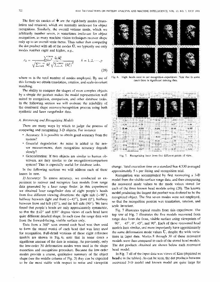
Data from a 360” scan around each head was then used to form the stored model of each head that was later used for recognition. Full-detail versions of these eight reference models are shown in Fig. 6; note that in some cases a significant amount of the data is missing. As previously, only the low-order 30 deformation modes were used in the shape extraction and recognit ion procedure. Because the low-order modes provide a coarse, qualitative summary of the object shape (see the middle column of Fig. 3) they can be expected to be the most stable with respect to noise and viewpoint

Fig. 6. Eight heads used in our recognition experiment. cases there is significant missing data.

Note that in some

Fig. 7. Recognizing faces from five different points of view.

change. Total execut ion time on a standard Sun 41330 averaged approximately 5 s per fitting and recognit ion trial.

Recognit ion was accompl ished by first recovering a 3-D model from the visible-surface range data, and then compar ing the recovered mode values to the mode values stored for each of the three known head models using (28). The known model producing the largest dot product was declared to be the recognized object. The first seven modes were not employed, so that the recognit ion process was translation, rotation, and scale invariant.

Fig. 7 illustrates typical results from this experiment. The top row of Fig. 7 illustrates the five models recovered from range data from the front, visible surface using viewpoints of -9O”, -45’, O”, 45”, and 90”. Each of these recovered head models look similar, and more importantly have approximately the same deformation mode values 0, despite the wide varia- tions in input data. Modes 8 through 30 of these recovered models were then compared to each of the stored head models. The dot products obtained are shown below each recovered head model.

In Fig. 7 all of the input data was views of Kim (depicted as head c in the tables). As can be seen, the dot products between recovered 3-D model and known model are quite large for


Kim’s head model. In fact, in this example the smallest correct dot product is almost three times the magni tude of any of the incorrect dot products; the same was also true for range data of the other subjects.

In this experiment 92.5% accurate recognit ion was obtained. That is, we successfully recovered 3-D models and recognized each of the eight test subjects from each of the five different views with only three errors. Analysis of the recognit ion results showed that, while the average dot product between different reference models was 0.31 (72’), the average dot product between models recovered from different views of the same person was 0.95 (18”). Thus recognit ion was typically extremely certain. All three errors were from front-facing views, where relatively few discriminating features are visible; remember that only overall head shape, and not details of surface shape, were available to the recognit ion procedure as only 30 modes were employed.

2) Graceful Degradation: Model recognit ion should not only be accurate, it should also be robust with respect to noise and sparsely sampled data. The next example, therefore, demonstrates robustness of recognit ion when using noisy data.

In this experiment the collection of relatively similar objects shown in the Fig. 2 were used to generate synthetic data with varying object orientation and varying degrees of noise. From this synthetic data 3-D models were recovered, and then recognized by compar ing the mode values of the recovered objects to those of the original objects. Again, translation, rotation, and scale invariant matching was employed.

W ithin each trial the 3-D orientation of each object was chosen from the entire viewing sphere at random, and the position of visible corners, edges, and face centers was measured, resulting in between 11 and 18 data points. Data points were then corrupted by adding uniformly distributed noise was to the data point’s x, y, and z coordinates. Note that only the front-facing 3-D points were used. The projection of data points onto the model was assumed to be known, so that the performance of the fitting and recognit ion algorithms could be evaluated independent ly of the moment method for estimating initial orientation. Total execut ion time on a standard Sun 4/330 is approximately 0.1 s per fitting and recognit ion trial.

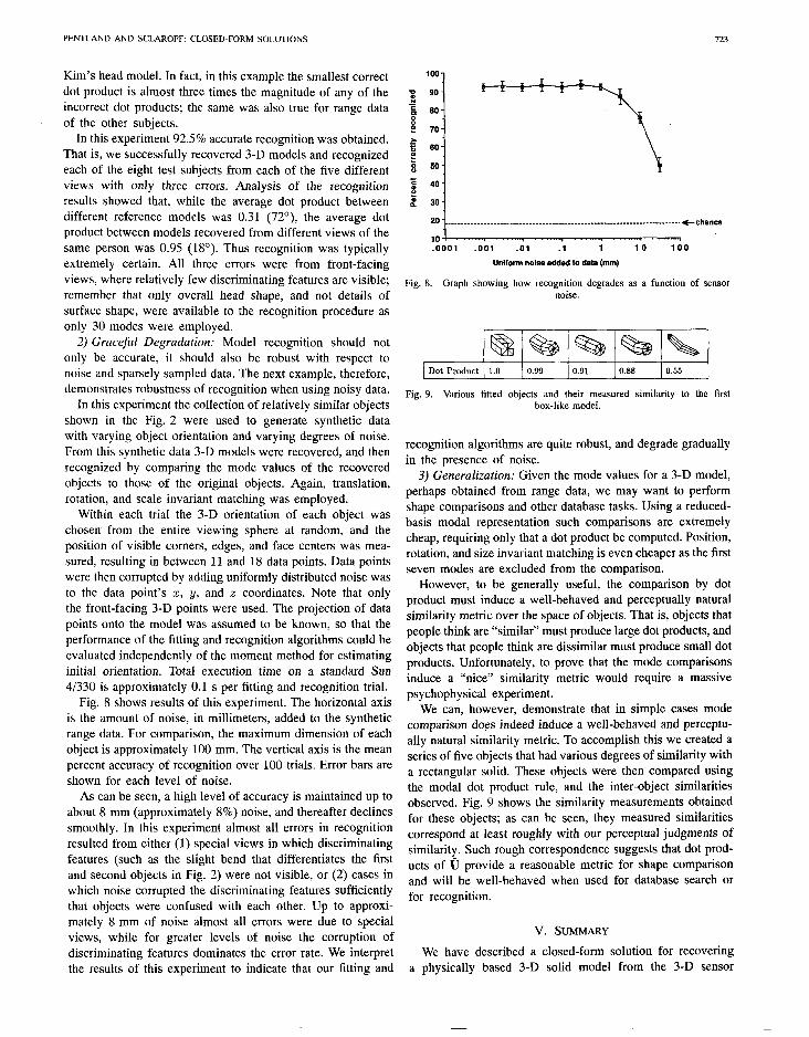
Fig. 8 shows results of this experiment. The horizontal axis is the amount of noise, in millimeters, added to the synthetic range data. For comparison, the maximum dimension of each object is approximately 100 mm. The vertical axis is the mean percent accuracy of recognit ion over 100 trials. Error bars are shown for each level of noise.

As can be seen, a high level of accuracy is maintained up to about 8 mm (approximately 8%) noise, and thereafter decl ines smoothly. In this experiment almost all errors in recognit ion resulted from either (1) special views in which discriminating features (such as the slight bend that differentiates the first and second objects in Fig. 2) were not visible, or (2) cases in which noise corrupted the discriminating features sufficiently that objects were confused with each other. Up to approximately 8 mm of noise almost all errors were due to special views, while for greater levels of noise the corruption of discriminating features dominates the error rate. W e interpret the results of this experiment to indicate that our fitting and

P 2 .z g 60- 8 z? 70 h = P 60

1 60-

= 40 E 2 30 1

20 _ -_-______-_ .----........-...----.....---------.---------.---------------~tchance

10 “‘..‘.I “““1 “““. . “‘..‘.- “..‘..‘I . ‘.‘-“I .OOOl .OOl .Ol .l 1 10 100

Uniform noise added to data (mm)

Fig. 8. Graph showing how recognition degrades as a function of sensor noise.

Dot Product 1.0 0.99 0.91 0.88 0.55

Fig. 9. Various fitted objects and their measured similarity to the first box-like model.

recognit ion algorithms are quite robust, and degrade gradually in the presence of noise.

3) Generalization: Given the mode values for a 3-D model, perhaps obtained from range data, we may want to perform shape compar isons and other database tasks. Using a reduced- basis modal representat ion such compar isons are extremely cheap, requiring only that a dot product be computed. Position, rotation, and size invariant matching is even cheaper as the first seven modes are excluded from the comparison.

However, to be general ly useful, the compar ison by dot product must induce a wel l -behaved and perceptual ly natural similarity metric over the space of objects. That is, objects that people think are “similar” must produce large dot products, and objects that people think are dissimilar must produce small dot products. Unfortunately, to prove that the mode compar isons induce a “nice” similarity metric would require a massive psychophysical experiment.

W e can, however, demonstrate that in simple cases mode compar ison does indeed induce a wel l -behaved and perceptu- ally natural similarity metric. To accomplish this we created a series of five objects that had various degrees of similarity with a rectangular solid. These objects were then compared using the modal dot product rule, and the inter-object similarities observed. Fig. 9 shows the similarity measurements obtained for these objects; as can be seen, they measured similarities correspond at least roughly with our perceptual judgments of similarity. Such rough cor respondence suggests that dot products of fi provide a reasonable metric for shape compar ison and will be wel l -behaved when used for database search or for recognition.

V. SUMMARY

W e have descr ibed a closed-form solution for recovering a physically based 3-D solid model from the 3-D sensor

724 IEEE TRANSACTIONS ON PAmERN ANALYSIS AND MACHINE INTELLIGENCE, VOL. 13, NO. 7, JULY 1991

measurements. In our current implementation we typically use 30 deformation modes, so that given as few as 11 independent 3-D sensor measurements the solution is overconstrained, and therefore unique except for rotational symmetries and degenerate conditions.

Because the recovered 3-D shape description is unique except for rotational symmetries, we may efficiently measure the similarity of different shapes by simply calculating normalized dot products between the mode values U of various objects. Such compar isons may be made position, orientation and/or size independent by simply excluding the first seven mode amplitudes. Thus the modal representat ion seems likely to be useful for applications such as object recognit ion and spatial database search.

The major weaknesses of our current method are l the need to estimate object orientation to within f15”, as

in our formulation rotational variation has been linearized. l The need to segment data into simple, approximately

convex “blobs” in a stable, viewpoint-invariant manner. In the current implementation of our system we use a standard method-of-moments to obtain initial estimates of object orientation, and a minimum description length technique to produce segmentat ions [17]. Using these techniques we have been able to obtain accurate, stable descriptions of shape for a wide variety of simple examples. For more complex scenes, however, considerable development of the segmentat ion and orientation modules will be required.

APPENDIX A FINITE ELEMENT METHOD FORMULATION

The finite element method (FEM) is a numerical procedure used in engineer ing analysis, particularly for relating the forces on and within a single object to its subsequent motion and deformation. This section presents the introductory concepts of the FEM by deriving the formulation of the mass and stiffness matrices. The formulations and examples presented here are based on those of Bathe [15] and Segerl ind [18], as summarized by Essa [19]. The notations used are compatible with Bathe [15].

This formulation is based on the fact that, when a certain part (node) of a body is al lowed some displacement U, it is possible to calculate the appl ied loads R acting upon it. This displacement-based finite element can then be extended to the general displacement method of analysis.

A. Formulation of Displacement-Based Finite Element Method

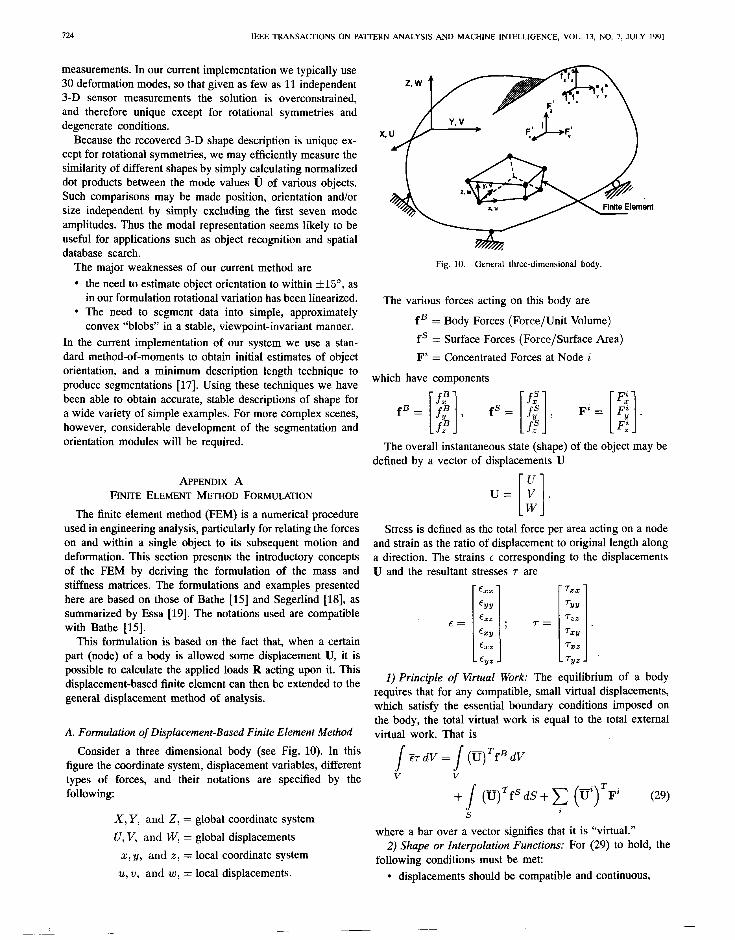
Consider a three dimensional body (see Fig. 10). In this figure the coordinate system, displacement variables, different types of forces, and their notat ions are specif ied by the following:

X, Y, and 2, = global coordinate system U, V, and W, = global displacements

z, y, and Z, = local coordinate system 21, u, and w, = local displacements.

X

Fig. 10. General three-dimensional body.

The various forces acting on this body are

fB = Body Forces (Force/Unit Volume) fS = Surface Forces (Force/Surface Area) Fi = Concentrated Forces at Node i

which have components

fB= [$I, fS= [g], Fi= [$I.

The overall instantaneous state (shape) of the object may be def ined by a vector of displacements U

Stress is def ined as the total force per area acting on a node and strain as the ratio of displacement to original length a long a direction. The strains e corresponding to the displacements U and the resultant stresses r are

%x Q-xx EYY TYY

En rzz .5= T= EXY 7XY

fxz - EY% :; 1:.

TX, rY%

1) Principle of Virtual Work: The equilibrium of a body requires that for any compatible, small virtual displacements, which satisfy the essential boundary condit ions imposed on the body, the total virtual work is equal to the total external virtual work. That is

/c7dV=/(u)TfBdV

V V

+/- (TQTfSdS+x (ti)TF’i (29) s i

where a bar over a vector signifies that it is “virtual.” 2) Shape or Interpolation Functions: For (29) to hold, the

following condit ions must be met: l displacements should be compatible and cont inuous,

PENTLAND AND SCLAROFF: CLOSED-FORM SOLUTIONS

l they must satisfy the displacement boundary conditions, W e can now derive K by substituting the stress-displacement and interpolation function (31) into (32) (and ignoring the initial

l they must satisfy constitutive relationships (i.e., stresses stress state for now) to obtain can be evaluated from strains).

Thus using the Principle of Virtual Work allows us to define r(i) = E(i)B(i)U. (35)

a system of shape functions that relate the displacement of Substituting this expression into the left-hand side of (34) to one node of the body with the relative displacements of all obtain the other nodes. Similar functions can be def ined for the distribution of strains across the body. These vector functions called the displacement interpolation functions and the strain- s

F(i)r(;) dV(i) = UT displacement interpolation functions, where Yt)

(J B&E(i)B(i) d yi;) U (36)

U(i) = H(i)U u(i) = H(i)U(i) (30) compar ing this equat ion with the steady-state equilibrium

are the displacement interpolation, and virtual displacement equat ion

interpolation functions and KU=R (37) qi) = B(i)U F(i) = B&j (31) where R is the vector of loads acting on each of the nodal

are the strain-displacement interpolation, and virtual strain- points, we obtain the stiffness matrix K displacement interpolation functions, where

H = The displacement interpolation matrix K=F/ BT-,)E(,)B(i) dV(i)* (38)

B = The strain-displacement matrix i V(t)

U = The three dimensional displacement vector i = The element number.

U is a dm x 1 vector, H is a dm x d matrix, and B is a dm x 2d matrix, where d is the dimensionality of the element, and m is the total number of elements in the assemblage. H and B are related and B can be calculated by appropriate differentiations of the functions in H, as is explained in the following subsections.

3) Developing Stiffness and Load Matrices: By using (30) and (31) we can assemble local elasticity matrices into a global stiffness matrix K. This is accompl ished as follows.

At a node the relation between the strain e(i) and its initial stress 71(i) is

r(i) = E(i)c(i) + rqi) (32)

where E is the elasticity matrix which relates local stresses to resultant local strains. In one dimension E is a scalar E called Young’s Modulus. In two dimensions, E is a 3 x 3 matrix relating stress and strain in the xy plane, e.g.,

By a similar substitution we can also obtain expressions for the load R on the r ight-hand side of (37) which is composed of body, surface, and concentrated load vectors, written RB, RS, and RC respectively, e.g.,

R=RB+RS+RC-RI (39)

where R’ is the vector of initial loads. These expressions are

(40)

RI = 2 J B&71(i) dyi) i V(t)

RC=F.

(42)

(43)

E E=- 4) Including Inertial Forces: In the above equat ions of mo- 1 - ua (33) tion, the effects of inertia were neglected. If a load is appl ied

rapidly, however, then inertial forces must be considered using where v is the material’s Poisson ratio, and in three dimensions d’Alambert’s principle. This can be accompl ished by simply E is a 6 x 6 matrix relating stress and strain in the x, y, z, including the element inertial forces as a part of the body and the three diagonal directions. forces

Mij+KU=R. (44) W e can then convert (29) into an element formulation

2 / z(i)r(i) dyi) = 2 / ($))‘f$ dqi) Assuming that the element accelerations are in the same

directions as the element displacements, the contribution of the inertia force to the load vector is


where p is the material-specific density. Thus we have that

5) Including Damping Forces: Over time, internal damping dissipates energy. This is taken into account by use of a velocity dependent damping force

Mij+CiJ+KU=R. (47)

Thus

(48)

where K is the material-specific internal damping constant. Thus we have

(49)

The following subsect ions present the complete method for setting up the stiffness K and mass M matrices including development of the shape interpolation functions.

B. Calculation of Mass, Damping, and Stiffness Matrices

W e will now develop the mass M, damping C, and stiffness K matrices for one, two, and three dimensional bodies. It will be assumed that the bodies are isoparametric, that is, that element displacements are interpolated in the same manner as the underlying coordinates. An example of a one-dimensional body will be given to provide a more intuitive idea of this method.

1) Setting up H and B Matrices: A Simple Example: First we need to define the H and B matrices which are used to determine M, C, and K. H and B are def ined in terms of a set of interpolation functions hi. The two major assumptions used to set up the interpolation functions hi are:

1) hi equals 1 at xi and equals 0 at every other node. 2) Sum of interpolation functions is always equal to 1.0

(that is, C hi = 1.0). Using these assumptions the interpolation functions hi,

and thus the H and B matrices, can be determined. This is illustrated by the following simple examples.

Example 1: A one dimensional bar element: In the figure of a beam element shown in Fig. 11 a new form of local coordinates is introduced, which sets up a system that is easy to integrate. The local coordinates vary from -1.0 to 1.0 in ‘r’ in the direction of X.

Transformation from the local r-coordinate system to the global X-coordinate system is given by

x = f (1 - T-)X1 -t a (1+ r)Xa.

Now let

hI = ; (1 - r), h2 = $ (1 + r)

I I I Fig. 11. A simple bar element.

therefore

X = hlXl + h2X2.

Similarly, as we are deal ing with an isoparametric element, the displacements are

U = hlUl + hzU2.

Using (30) we see that hI and h2 are simply the interpolation functions for node 1 and 2, respectively, hence

HT= $(1++r) . 1 Substituting into (46) and (49)

and

where A is the cross-sectional area of the beam. W e next need to determine B. By definition

dU dU dr E=-=-- dX dr dX

dU u2 - fJ1

dr= 2

and thus, from Fig. 11 we obtain %, also referred to as the Jacobian J

W e can now set up equat ions for e and, using (31) also for B

u2 Ul E=--- L L

B= -;+. [ 1 By substituting into (38) for m = 1, and by using the result that for a one-dimensional element E = E, where E is Young’s modulus, we have

K=/ [-~],[t+]AdX.

One of the reasons for defining a new coordinate system of r is for ease of integration. If in the above equat ion of M, C,


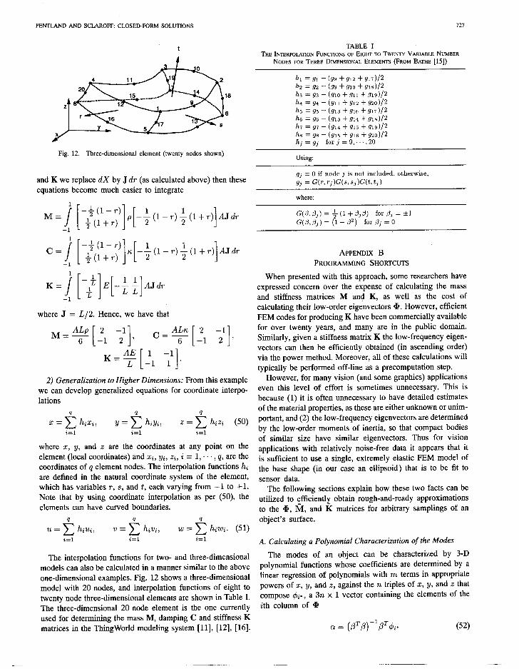
18

8

Fig. 12. Three-dimensional element (twenty nodes shown)

and K we replace dX by J dr (as calculated above) then these equations become much easier to integrate

where J = Lf 2. Hence, we have that

M-A-b 6

[ 2 -1 -1 2

1 ’

K = y J1 1’ . [ 1 2) Generalization to Higher Dimensions: From this example

we can develop generalized equations for coordinate interpo- lations

q x= c hixi, Y = & byi, .Z= 2 hiz; (50) i=l i=l i=l

where x, y, and z are the coordinates at any point on the element (local coordinates) and xi, yi, zi, i = 1, s . . , q, are the coordinates of q element nodes. The interpolation functions hi are defined in the natural coordinate system of the element, which has variables T, s, and t, each varying from -1 to +l. Note that by using coordinate interpolation as per (50), the elements can have curved boundaries.

Q Q u= c hiui, v= c hivi, w= 2 hiwi. (51)

i=l i=l i=l

The interpolation functions for two- and three-dimensional models can also be calculated in a manner similar to the above one-dimensional examples. Fig. 12 shows a three-dimensional model with 20 nodes, and interpolation functions of eight to twenty node three-dimensional elements are shown in Table I. The three-dimensional 20 node element is the one currently used for determining the mass M, damping C and stiffness K matrices in the ThingWorld modeling system [ll], [12], [16].

TABLE I THE INTERPOLATION FUNCTIONS OF EIGHT TO TWENTY VARIABLE NUMBER

NODES FOR THREE DIMENSIONAL ELEMENTS (FROM BATHE [15])

hl = 91 - (s9 + 912 + 917)/2 b2 = 92 - (g9 + 910 + 918)P h3 = 93 - (910 + 911 + 919)P h4 = 94 - (911 + 912 + 920)/2 h5 = g5 - (913 + 916 + g17)/2 h6 = 96 - (913 + 914 + gl8)/2 h7 = 97 - (914 + 915 + g19)/2 h8 = $78 - (915 +glS +920)/x h, = gj for j = 9, ” ) 20

Using:

gj = 0 if node j is not included, otherwise, gj = G(r,rj)G(s,sj)G(t,t3)

where:

APPENDIX B PROGRAMMING SHORTCUTS

When presented with this approach, some researchers have expressed concern over the expense of calculating the mass and stiffness matrices M and K, as well as the cost of calculating their low-order eigenvectors 9. However, efficient FEM codes for producing K have been commercially available for over twenty years, and many are in the public domain. Similarly, given a stiffness matrix K the low-frequency eigenvectors can then be efficiently obtained (in ascending order) via the power method. Moreover, all of these calculations will typically be performed off-line as a precomputation step.

However, for many vision (and some graphics) applications even this level of effort is sometimes unnecessary. This is because (1) it is often unnecessary to have detailed estimates of the material properties, as these are either unknown or unimportant, and (2) the low-frequency eigenvectors are determined by the low-order moments of inertia, so that compact bodies of similar size have similar eigenvectors. Thus for vision applications with relatively noise-free data it appears that it is sufficient to use a single, extremely elastic FEM model of the base shape (in our case an ellipsoid) that is to be fit to sensor data.

The following sections explain how these two facts can be utilized to efficiently obtain rough-and-ready approximations to the @, a, and K matrices for arbitrary samplings of an object’s surface.

A. Calculating a Polynomial Characterization of the Modes

The modes of an object can be characterized by 3-D polynomial functions whose coefficients are determined by a linear regression of polynomials with m terms in appropriate powers of x, y, and z, against the n triples of x, y, and z that compose $i*, a 3n x 1 vector containing the elements of the ith column of Cp

0. = (~‘p)-‘~‘$i*

728 IEEF TRANSACTIONS ON PATTERN ANALYSIS AND MACHINE INTELLIGENCE, VOL. 13, NO. 7, JULY 1991

where cx is an m x 1 matrix of the coefficients of the desired deformation polynomial, /3 is a 3n x m matrix whose first column contains the object-centered coordinates of the nodes (LC~,Y~;Z~.~~:Z.Y~,Z~....,~~,Y~,~~)~, and whose remaining columns consist of the modif ied versions of the nodal coordinates where the Z, y, and/or z components have been raised to various powers. See [12] for more details.

By linearly super imposing the various deformation map- pings, one can obtain an accurate account ing of the object’s nonrigid deformation. In the ThingWorld model ing system [I2], [16] the set of polynomial deformations is combined into a 3 by 3 matrix of polynomials, D, that is referred to as the modal deformation matrix. This matrix transforms pre- deformation point posit ions X = (z. y, ~)r into the deformed posit ions

A simple version of D that is der ived from a 20 node element is given by the following:

do0 = 67 + ?/UT13 + zii16 - (ii14 + tirr)sgn(z) - Cr5 - iLrs,

do1 = G;;-~z +2y(ti14 +~gn(x)iil~),

do2 = Ull + 2z(Urr + sgn(z)ir.rs), d,, = GIZ + 25(&o + sgn(y)uzl), dll = jig + x2119 + 2522 - (tizo + &s)sgn(y) - ii21 - U24, dl2 = ti10 + 22(&s + sgn(y)&), &to = iill + k(c26 + sgn(z)&), 61 = 610 + 2y(G+ + w(z)&), d22 = ‘iit, + x’ii25 + vii28 - (‘ii26 + ‘629)Sgn( z) - ‘ii27 - 630.

(54)

W e have found that this characterization of mode shapes provides a reasonable description of the behavior of the ellipsoids used in our fitting process.

The modal ampli tudes Gi have intuitive meanings: 1Lr-46 are the rigid body modes (translation and rotation), ‘21749 are the Z, y, and z radius, i;Lra-tit2 are shears about the x, y, and Z axes, and ‘i&+sj-&a+sj+2 may be descr ibed as tapering, bending, and pinching around the jth pairwise combinat ion of the x, y, and z axes. Note that because the rigid body modes are calculated in the object’s coordinate system, they must be rotated to global coordinates before being integrated with the remainder of any dynamical simulation.

B. Approximate Calculation of 9, %I, and l%

W e can make use of the above mode characterization to numerically approximate the matrix + for any point sampling of the surface. In essence, we are precalculating how energy in each of the various modes displaces of a set of points on the surface. W e then store this mode-displacement relationship into the + matrix, thus approximating how these points distribute load to the original nodal points and the various vibration modes.

This numerical approximation is accompl ished by noting that &- (the %th column of a) descr ibes how the n nodal points X”’ = (xy , y,W, z?)’ change with ui, the ith mode’s amplitude

Thus by applying small amount of each deformation iGi and measur ing the resulting change in the coordinates of each surface point as it is passed through (53), we obtain finite difference approximations to the (j + 1, i), (j + 2, i) and (j + 3, i) entries of * for any sampling of surface points.

W e can use this method to efficiently obtain a sampling of the surface that matches the projection of the sensor data onto the surface, thus considerably simplifying the fitting process. Even when iterating the solution to find better virtual spring attachment points, the distances between nodes and projected data posit ions will be small, and so simple bilinear interpolation can be used to distribute the data forces to the surrounding three surface points without incurring significant error.

Given a @ with nodes evenly sampled throughout the body, we can use the common assumption that the object’s mass is distributed equally among the sampled points to obtain

ti = aTM@ = eTmI+ (56)

where m is the mass assigned to each sample point. The modal stiffnesses ,& are more difficult to estimate; however, given that detailed material propert ies are unimportant, one may simply assign a stiffness proport ional to &i for the nonrigid modes 1Li, and a stiffness of 0.0 for the rigid-body modes Ici, 1 < i < 6. -

C. Surface Detail Description

In the ThingWorld system [12], [16] the low-order modal representat ion is augmented by a surface mesh description of the surface’s detailed structure, in order to obtain a more general shape representation. This spline description can be either a physically based mesh, or a simple spline. The basic idea is to replace the implicit function description f(x, y, z) = d = 1 with the more general implicit function f (x, y, z) = d(x, y, 2). This allows us to capture more detailed structure than is possible with any fixed number of modes without losing the advantages of an implicit function representation. The surface details are normally treated as error residuals relative to the model’s dynamic behavior, a l though they are used in point, ray, or surface intersection calculations.

ACKNOWLEDGMENT

The authors would like to thank I. Essa for his summary of Bathe and Segerlind, from which Section II-A and Appendix A were derived, and for his proofreading.

REFERENCES

(11 T. Binford, “Visual perception by computer,” presented at the IEEE conference on Systems and Control, Dec. 1971.


PI

[31

[41

[51

[cl

[71

PI

[91

WI

[Ill

[121

(131

[I41

1151

[1’51

D. Marr and K. Nishihara, “Representation and recognition of the spatial organization of three-dimensional shapes,” in Proc. of the Royal Society-London B, 1978. R. Mohan and R. Nevatia, “Using perceptual organization to extract 3D structures,” IEEE Trans. Putt. Anal. Mach. Intell., vol. 11, no. 11, pp. 1121-1139, Nov. 1989. A. Pentland, “Perceptual organization and representation of natural form,” Artificial Intell., vol. 28, no. 3, pp. 293-331, 1986. A. Pentland, “Recognit ion by parts, ” in Proc. First International Conf Comput. Vision, (London, England), 1987, pp. 612-620. F. Solina and R. Bajcsy, “Recovery of parametric models from range images: The case for superquadrics with global deformations,” fEEE Trans. Patt. Anal. Mach. Intell.. vol. 12, no. 2, pp. 131-147, 1990. T. Boult and A. Gross, “Recovery of superquadrics from depth information,” in Proc. of the AAAI Workshop on Spatial Reasoning and Multi-Sensor Fusion, Oct. 1987, pp. 128- 137. I. Biederman, “Recognit ion-bv-comnonents: A theorv of human image understanding,” Psychologicai Rev., ‘vol. 94, no. 2, pp. 115 - 147, 1987. P. Winston, T. Binford, B. Katz, and M. Lowry, “Learning physical description from functional descriptions, examples, and precedents,” in Proc. if AAAI, 1983, pp. 433-439. D. Terzopoulos, A. Witkin, and M. Kass, “Symmetry-seeking models for 3-D object reconstruction,” ht. J. Comput. Vision, vol. 1, no. 3, pp. 211-221, 1987. A. Pentland, “Automatic extraction of deformable part models,” Inter- national J. Comput. Vision, pp. 107- 126, 1990. A. Pent land and J. Will iams, “Good vibrations: Modal dynamics for graphics and animation,” Comput. Graphics, vol. 23, no. 4, pp. 215-222, 1989. M. Leyton, “Perceptual organization as nested control,” Biological Cybernetics, vol. 51, pp. 141-153, 1984. D. Hoffman and W. Richards, “Parts of recognition,” in From Pixels to Predicates (A. Pentland, Ed.). Norwood, NJ: Ablex, 1985. K. Bathe, Finite Element Procedures in Engineering Analysis. Engle- wood Cliffs, NJ: Prentice-Hall, 1982. A. Pentland, I. Essa, M. Freidmann, B. Horowitz, and S. Sclaroff, “The thinaworld model ing system: Virtual sculpting bv modal forces,” Comput. Graphics, vol. 2<, no. 2, pp. 143-144, 1990: T. Darrell. S. Sclaroff, and A. Pentland, “Segmentat ion by minimal description,” in Proc. Third International Conf Comput. &ion, Dec. 1990.

Alex Pent land received the Ph.D. degree from the Massachusetts Institute of Technology, Cambridge, in 1982.

Subsequently, he began working at SRI Interna- tional’s Artificial Intell igence Center. He was appointed Industrial Lecturer in Stanford Universities’ Computer Science Department in 1983, winning the Distinguished Lecturer award in 1986. In 1987, he was appointed Associate Professor of Computer, In- formation, and Design Technology at MIT’s Media Laboratory and was given the NEC Computer and

Communicat ions Career Development Chair in 1988. He has done research in artificial intelligence, machine vision, human vision, and computer graphics.

Dr. Pent land won the Best Paper Prize from the American Association for Artificial Intell igence for his fractal textures research in 1984 and the Best Paper Prize from the IEEE for his face recognition research in 1991. His last book was entitled From Pixels to Predicates (Norwood, NJ: Ablex) and is currently working on one entitled Dynamic Vision, to be publ ished by Bradford Books, MIT Press.

Stan Sclaroff (M’90) received the B.S. degree in computer science and english from Tufts University, Medford, MA, in 1984. He is currently a graduate student and a research assistant in the Vision and Model ing Group at the MIT Media hbOratOry and is expected to receive the M.S. degree from the Massachusetts Institute of Technology in May, 1991.

Previously, he has been a Senior Software Engi- neer in the solids model ing and computer graphics groups at Schlumberger Technologies, CAD/CAM

L. Segerlind, Appl ied Finite ElementAnalysis. New York: Wiley, 1984. Division, in Billerica, MA. HIS research Interests are m computer vtsron, I. Essa. “Contact Detection. Collision Forces, and Friction for Phvsically- computer graphics, physically based model ing, computer a ided design, and Based Virtual World Model ing,” M.A. thesis, Dept. of Civil Engineering, computat ionai geometry. M.I.T., 1990. Mr. Sclaroff is a student member of the ACM.

IEEE TRANSACTIONS ON PATTERN ANALYSIS AND …cns.bu.edu/~gsc/Articles/Scarloff_Shape_FEM.pdfIEEE...

Documents

Transcript of IEEE TRANSACTIONS ON PATTERN ANALYSIS AND …cns.bu.edu/~gsc/Articles/Scarloff_Shape_FEM.pdfIEEE...