IEEE TRANSACTIONS ON IMAGE PROCESSING, VOL. 20, NO. 12, DECEMBER 2011 1

Generalized Random Walks for Fusion ofMulti-Exposure Images

Rui Shen, Student Member, IEEE, Irene Cheng, Senior Member, IEEE, Jianbo Shi,and Anup Basu, Senior Member, IEEE

Abstract—A single captured image of a real-world scene isusually insufficient to reveal all the details due to under- or over-exposed regions. To solve this problem, images of the same scenecan be first captured under different exposure settings and thencombined into a single image using image fusion techniques. Inthis paper, we propose a novel probabilistic model-based fusiontechnique for multi-exposure images. Unlike previous multi-exposure fusion methods, our method aims to achieve an optimalbalance between two quality measures, i.e., local contrast andcolor consistency, while combining the scene details revealed un-der different exposures. A generalized random walks frameworkis proposed to calculate a globally optimal solution subject tothe two quality measures by formulating the fusion problemas probability estimation. Experiments demonstrate that ouralgorithm generates high-quality images at low computationalcost. Comparisons with a number of other techniques show thatour method generates better results in most cases.

Index Terms—Image fusion, multi-exposure fusion, randomwalks, image enhancement.

I. INTRODUCTION

A natural scene often has a high dynamic range (HDR) thatexceeds the capture range of common digital cameras.

Therefore, a single digital photo is often insufficient to provideall the details in a scene due to under- or over-exposed regions.On the other hand, given an HDR image, current displays areonly capable of handling a very limited dynamic range. Inthe last decade, researchers have explored various directionsto resolve the contradiction between the HDR nature of real-world scenes and the low dynamic range (LDR) limitationof current image acquisition and display technologies. Al-though cameras with spatially varying pixel exposures [1],cameras that automatically adjust exposure for different partsof a scene [2], [3], and displays that directly display HDRimages [4] have been developed by previous researchers, theirtechnologies are only at a prototyping stage and unavailableto ordinary users.

Instead of employing specialized image sensors, an HDRimage can be reconstructed digitally using HDR reconstruction(HDR-R) techniques from a set of images of the same scenetaken by a conventional LDR camera [5] or a panoramic

Copyright (c) 2011 IEEE. Personal use of this material is permitted.However, permission to use this material for any other purposes must beobtained from the IEEE by sending a request to pubs-permissions@ieee.org.

R. Shen, I. Cheng, and A. Basu are with the Department of ComputingScience, University of Alberta, Edmonton, AB, Canada T6G 2E8 (e-mail:rshen@ualberta.ca; locheng@ualberta.ca; basu@ualberta.ca).

J. Shi is with the Department of Computer and Information Sci-ence, University of Pennsylvania, Philadelphia, PA, USA 19104 (e-mail:jshi@cis.upenn.edu).

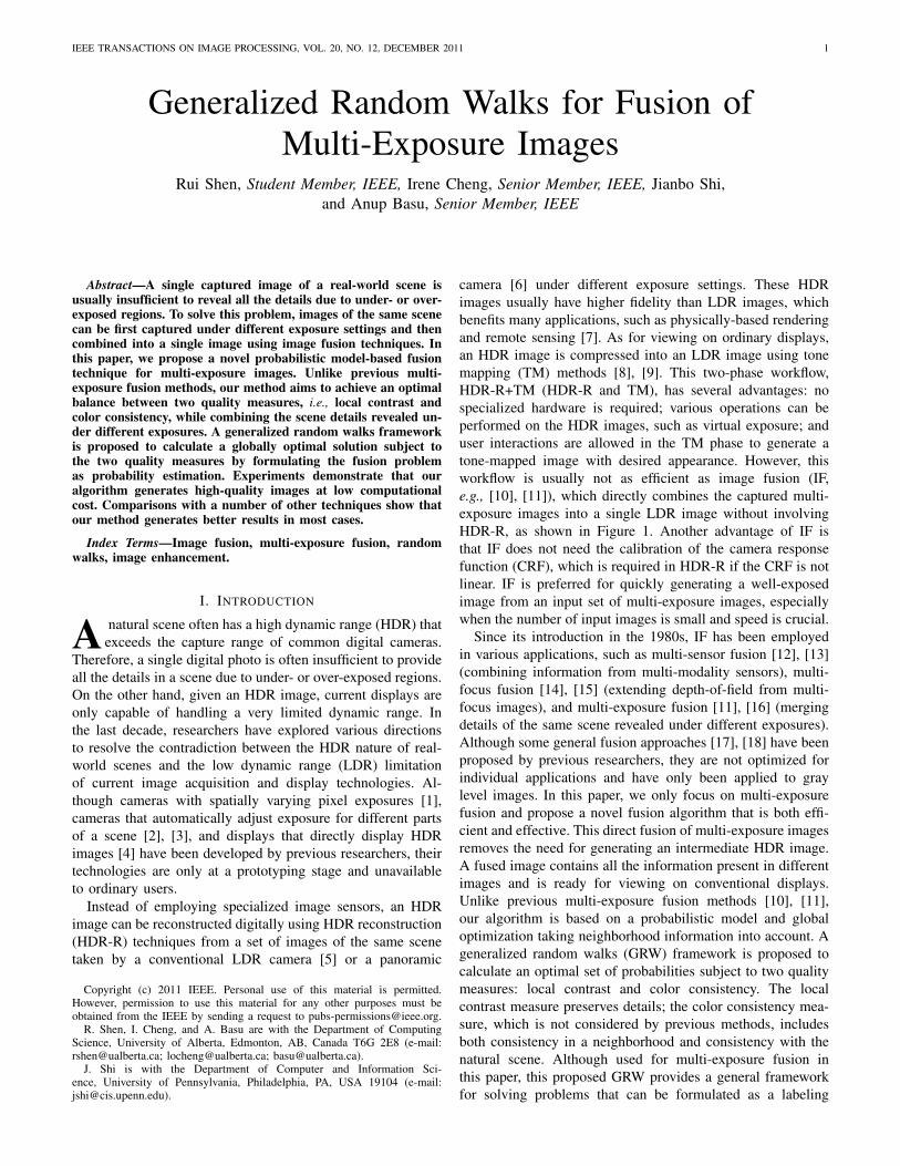
camera [6] under different exposure settings. These HDRimages usually have higher fidelity than LDR images, whichbenefits many applications, such as physically-based renderingand remote sensing [7]. As for viewing on ordinary displays,an HDR image is compressed into an LDR image using tonemapping (TM) methods [8], [9]. This two-phase workflow,HDR-R+TM (HDR-R and TM), has several advantages: nospecialized hardware is required; various operations can beperformed on the HDR images, such as virtual exposure; anduser interactions are allowed in the TM phase to generate atone-mapped image with desired appearance. However, thisworkflow is usually not as efficient as image fusion (IF,e.g., [10], [11]), which directly combines the captured multi-exposure images into a single LDR image without involvingHDR-R, as shown in Figure 1. Another advantage of IF isthat IF does not need the calibration of the camera responsefunction (CRF), which is required in HDR-R if the CRF is notlinear. IF is preferred for quickly generating a well-exposedimage from an input set of multi-exposure images, especiallywhen the number of input images is small and speed is crucial.

Since its introduction in the 1980s, IF has been employedin various applications, such as multi-sensor fusion [12], [13](combining information from multi-modality sensors), multi-focus fusion [14], [15] (extending depth-of-field from multi-focus images), and multi-exposure fusion [11], [16] (mergingdetails of the same scene revealed under different exposures).Although some general fusion approaches [17], [18] have beenproposed by previous researchers, they are not optimized forindividual applications and have only been applied to graylevel images. In this paper, we only focus on multi-exposurefusion and propose a novel fusion algorithm that is both effi-cient and effective. This direct fusion of multi-exposure imagesremoves the need for generating an intermediate HDR image.A fused image contains all the information present in differentimages and is ready for viewing on conventional displays.Unlike previous multi-exposure fusion methods [10], [11],our algorithm is based on a probabilistic model and globaloptimization taking neighborhood information into account. Ageneralized random walks (GRW) framework is proposed tocalculate an optimal set of probabilities subject to two qualitymeasures: local contrast and color consistency. The localcontrast measure preserves details; the color consistency mea-sure, which is not considered by previous methods, includesboth consistency in a neighborhood and consistency with thenatural scene. Although used for multi-exposure fusion inthis paper, this proposed GRW provides a general frameworkfor solving problems that can be formulated as a labeling

2 IEEE TRANSACTIONS ON IMAGE PROCESSING, VOL. 20, NO. 12, DECEMBER 2011

HDRreconstruction

Tone mapping

Multi-exposure LDR images

Single HDR image

Multi-exposure fusion

Single LDR image

Fig. 1. Comparison between multi-exposure fusion and the HDR reconstruction and tone mapping workflow. (The Garage image sequence courtesy of ShreeNayar.)

problem [19], i.e., estimating the probability of a site (e.g., apixel) being assigned a label based on known information. Theproposed fusion algorithm has low computational complexityand produces a final fused LDR image with fine details and anoptimal balance between the two quality measures. By definingproblem-specific quality measures, the proposed algorithmmay also be applied to other fusion problems.

The rest of the paper is organized as follows. Section IIreviews previous methods. Differences between our algorithm,previous IF methods, and methods used in the HDR-R+TMworkflow, are also discussed. Section III explains our algo-rithm in detail. Section IV discusses experimental results andperformance, along with comparisons with other IF methodsand the HDR-R+TM workflow. Finally, Section V gives theconclusions and future work.

II. RELATED WORK

A. Multi-Exposure Image Fusion

Image fusion methods combine information in differentimages into a single composite image. Here we only discussthose IF methods that are most relevant to our algorithm.Please refer to [20] for an excellent survey on IF methods indifferent applications. For multi-exposure images, IF methodsdirectly work on the input LDR images and focus on enhanc-ing dynamic range while preserving details. Goshtasby [10]partitions the input images into uniform blocks and tries tomaximize the information in each block based on an entropymeasure. However, the approach may generate artifacts onobject boundaries if the block is not sufficiently small. Insteadof dividing images into blocks, Cheng and Basu [21] combineimages in a column-by-column fashion. This algorithm max-imizes the contrast within a column by selecting pixels fromdifferent images. However, since no neighborhood informationis considered, it cannot preserve color consistency and artifactsmay occur on object boundaries. Cho and Hong [22] focuson substituting the under- or over-exposed regions in oneimage, which are determined by a saturation mask, with thewell-exposed regions in another image. Region boundariesare blended by minimizing an energy function defined inthe gradient domain. Although this algorithm works betteron object boundaries, it is only applicable to two images.Our algorithm works at the pixel level and applies a globaloptimization taking neighborhood information into account,which avoids the boundary artifacts.

Image fusion can also be interpreted as an analogy toalpha blending. Raman and Chaudhuri [23] generate the fusedimage by solving an unconstrained optimization problem. Theweight function for each pixel is modeled based on localcontrast/variance in a way that the fused image tends to haveuniform illumination or contrast. Raman and Chaudhuri [24]generate mattes for each pixel in an image using the differencebetween the original pixel value and the pixel value afterbilateral filtering. This measure strengthens weak edges, butmay not be sufficient to enhance the overall contrast. Ouralgorithm defines two quality measures and finds the optimalbalance between them, i.e., enhancing local contrast whileimposing color consistency.

Multi-resolution analysis based fusion has demonstratedgood performance in enhancing main image features. Bogoniand Hansen [16] propose a pyramid-based pattern-selectivefusion technique. Laplacian and Gaussian pyramids are con-structed for the luminance and chrominance components,respectively. However, the color scheme of the fused imagemay be very close to the average image because pixels withsaturation closest to the average saturation are selected forblending. Mertens et al. [11] construct Laplacian pyramids forthe input images and Gaussian pyramids for the weight maps.A weight for a pixel is determined by three quality measures:local contrast, saturation, and well-exposedness. The Laplacianand Gaussian pyramids are blended at each level, and thencollapsed to form the final image. However, with only localcalculation involved and no measure to preserve color con-sistency, the fusion results may be unnatural. Our algorithmalso uses local contrast as one quality measure, but anotherquality measure that we consider is color consistency, whichis not employed by [11]. Moreover, our algorithm does notuse pyramid decomposition but solves a linear system definedat the pixel level.

B. HDR Reconstruction and Tone MappingAlthough the HDR-R+TM workflow is usually used in

different scenarios than IF methods, we still give a briefdiscussion on those HDR-R and TM methods sharing somesimilar features to our IF algorithm, because the originalinput and the final output of this workflow is the same as IF.Given an input LDR sequence and exposure times associatedwith each image in the sequence, HDR-R techniques [5] firstrecover the CRF, which is a mapping from the exposure at eachpixel location to the pixel’s digital LDR value and then use the

SHEN et al.: GENERALIZED RANDOM WALKS FOR FUSION OF MULTI-EXPOSURE IMAGES 3

Computecompatibilities Optimize Fuse

Input images Initial probability maps Final probability maps Fused image

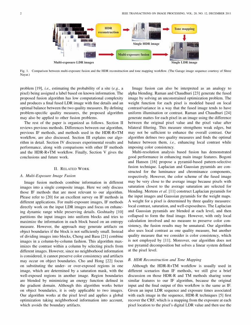
Fig. 2. Processing procedure of the proposed fusion algorithm. (The Window image sequence courtesy of Shree Nayar.)

CRF to reconstruct an HDR image via a weighting function.Debevec and Malik [5] recover the CRF by minimizing aquadratic objective function defined on exposures, pixels’ LDRvalues, and exposure times. Then, a hat-shaped weightingfunction is used to reconstruct the HDR image. Granados etal. [25] assume the CRF is linear and focus on the developmentof an optimal weighting function using a compound-Gaussiannoise model. Our IF algorithm also solves a quadratic objectivefunction, but the function is defined on local features and thesolution leads to probability maps.

Given an HDR image, tone mapping methods [26] aimto reduce its dynamic range while preserving details. TMusually works solely in the luminance channel. Global TMmethods [27], [28], which apply spatially invariant mappingof luminance values, usually have high speed, while local TMmethods [8], [9], [29], [30], which apply spatially varyingmapping, usually produce images with better qualities espe-cially when strong local contrast is present [9], [30]. Reinhardet al. [9] uses a multiscale local contrast measure to compressthe luminance values. Li et al. [29] decompose the luminancechannel of the input HDR image into multiscale subbands andapply local gain control to the subbands. Shan et al. [30]define a linear system for each overlapping window in theHDR image using local contrast, and the solution of eachlinear system are two coefficients that map luminance valuesfrom HDR to LDR. Although our IF algorithm also useslocal contrast to define a linear system, the local contrast inour algorithm is calculated in a different manner and anotherquality measure (i.e., color consistency) is also considered.Furthermore, our IF algorithm defines a linear system onpixels from all the original LDR images, and the solution isa set of probabilities that determine the contributions fromeach pixel of each original LDR image to its correspondingpixel in the fused image. Krawczyk et al. [8] segment anHDR image into frameworks with consistent luminance andcompute the belongingness of each pixel to each frameworkusing the framework’s centroid, which results in a set ofprobability maps. Our IF algorithm also generates probabilitymaps, but directly from the original LDR sequence with noHDR or segmentation involved. One typical problem withsome local TM methods is halo artifacts introduced due tocontrast reversals [26]. Our IF algorithm balances betweencontrast and consistency in a neighborhood, which can prevent

contrast reversals. Another problem with some TM methods isthat color artifacts like oversaturation may be introduced intothe results, because operations are usually performed in theluminance channel without involving chrominance [26]. Thisproblem does not apply to our IF algorithm, because everycolor channel is treated equally.

III. PROBABILISTIC FUSION

Unlike most previous multi-exposure fusion methods, weconsider image fusion as a probabilistic composition process,as illustrated in Figure 21. The initial probability that a pixelin the fused image belongs to each input image is estimatedbased on local features. Taking neighborhood informationinto account, the final probabilities are obtained by globaloptimization using the proposed generalized random walks.These probability maps serve as weights in the linear fusionprocess to produce the fused image. In a probability map, thebrighter a pixel is, the higher the probability. These processesare explained in detail below.

A. Problem Formulation

The fusion of a set of multi-exposure images can beformulated as a probabilistic composition process. Let D ={I1, . . . IK} denote the set of input images and L ={l1, . . . , lK} the set of labels, where a label lk ∈ L isassociated with the kth input image Ik ∈ D. Ik’s are assumedto be already registered and have the same size with N pixelseach. Normally, K � N . Let us define a set X of variablessuch that an xi ∈ X is associated with the ith pixel pi in thefused image I∗ and takes a value from L. Then, each pixel inthe fused image I∗ can be represented as:

pi =

K∑k=1

P k(xi)pki , (1)

where pki denotes the ith pixel in Ik and P k(xi) , P (xi =lk|D) the probability of pixel pi being assigned label lkgiven D with

∑k P

k(xi) = 1. This probabilistic formulationconverts the fusion problem to the calculation of marginalprobabilities given the input images subject to some qualitymeasures and helps to achieve an optimal balance between

1The initial probability maps are normalized at each pixel.

4 IEEE TRANSACTIONS ON IMAGE PROCESSING, VOL. 20, NO. 12, DECEMBER 2011

different quality measures. If every pixel is given equal prob-ability, i.e., P k(xi) = 1

K ,∀i, k, I∗ is simply the average ofIk’s. Although it is also possible to only combine pixels withhighest probabilities instead of using Equation (1), artifactsmay appear at locations with significant brightness changesbetween different input images.

If P k(xi)’s are simply viewed and calculated as localweights followed by applying some relatively simple smooth-ing filters, such as Gaussian filter and bilateral filter, eitherartifacts (like halos) may appear at object boundaries orit is difficult to determine the termination criteria of thefiltering, therefore the results are usually unsatisfactory [11].An alternative is to use multi-resolution fusion techniques [11],[16], where the weights are blended in each level to producemore satisfactory results. However, the weights in each levelare still determined locally, which may not be optimal in alarge neighborhood. In contrast to multi-resolution techniques,we propose an efficient single-resolution fusion technique byformulating P k(xi)’s in Equation (1) as probabilities in GRW.A set of optimal P k(xi)’s that balances the influence of dif-ferent quality measures is computed from global optimizationin GRW. Experiments (Section IV) show that the results ofthe proposed probabilistic fusion technique are comparable tothe results of multi-resolution techniques and the results of theHDR-R+TM workflow.

B. Generalized Random Walks

In this section, we propose a generalized random walks(GRW) framework based on the random walks (RW) al-gorithm [31], [32] and the relationship between RW andelectrical networks [33].

yjK

wijxi xj

lK... ...l1

Fig. 3. The graph used in GRW. The yellow nodes are scene nodes and theorange nodes are label nodes.

1) Image Representation: As shown in Figure 3, the vari-able set X and the label set L are represented in a weightedundirected graph similar to [31]. Each variable is associatedwith a pixel location, and each label is associated with aninput image in our case. The graph G = (V, E) is constructedas V = L∪X and E = V ×V including edges both within Xand between X and L. The yellow nodes are scene nodes andthe orange nodes are label nodes. For a scene node x ∈ X ,edges EX are drawn between it and each of its immediateneighbors in X (4-connectivity is assumed in our case). Inaddition, edges EL are drawn between a scene node and eachlabel node. wij , w(xi, xj) is a function defined on EX thatmodels the compatibility/similarity between nodes xi and xj ,

and yik , y(xi, lk) is a function defined on EL that modelsthe compatibility between xi and lk.

2) Dirichlet Problem: Let V be arranged in a way that thefirst K nodes are label nodes, i.e., {v1, . . . , vK} = L, and therest N nodes are scene nodes, i.e., {vK+1, . . . , vK+N} = X .With two positive coefficients γ1 and γ2 introduced to balancethe weights between y(·, ·) and w(·, ·), we can define a nodecompatibility function c(·, ·) on E with the following form:

cij , c(vi, vj) =

{γ1yi−K,j , (vi, vj) ∈ EL ∧ vj ∈ L;γ2wi−K,j−K , (vi, vj) ∈ EX .

(2)Because the graph is undirected, we have cij = cji. Letu(vi) denote the potential associated with vi. Based on therelationship between RW and electrical networks [33], the totalenergy of the system given in Figure 3 is:

E =1

2

∑(vi,vj)∈E

cij(u(vi)− u(vj))2. (3)

Our goal is to find a function u(·) defined on X that minimizesthis quadratic energy with boundary values u(·) defined on L.If u(·) satisfies O2u = 0, then it is called harmonic, and theharmonic function is guaranteed to minimize such quadraticenergy E [32]. The problem of finding this harmonic functionis called the Dirichlet problem.

The harmonic function u(·) can be computed efficientlyusing matrix operations. Similar to [32], a Laplacian matrixL can be constructed following Equation (4); however, un-like [32], L here contains both the label nodes and the scenenodes and becomes a (K +N)× (K +N) matrix:

Lij =

di, i = j;−cij , (vi, vj) ∈ E ;0, otherwise.

(4)

where di =∑vj∈Ni

cij is the degree of the node vi definedon its immediate neighborhood Ni. Then, Equation (3) can berewritten in matrix form as:

E =

(uLuX

)TL

(uLuX

)=

(uLuX

)T (LL BBT LX

)(uLuX

)(5)

where uL = (u(l1), . . . , u(lK))T and uX =(u(x1), . . . , u(xN ))T ; LL is the upper left K ×K submatrixof L that encodes the interactions within L; LX is the lowerright N × N submatrix that encodes the interactions withinX ; and B is the upper right K × N submatrix that encodesthe interactions between L and X . Hence, the minimumenergy solution can be obtained by setting OE = 0 withrespect to uX , i.e., solving the following equation:

LXuX = −BTuL. (6)

In some cases, part of X may be already labeled. These pre-labeled nodes can also be represented naturally in the currentframework without altering the structure of the graph. Supposexi is one of the pre-labeled nodes and is assigned label lk.Then, we can simply assign a sufficiently large value to yikand solve the same Equation (6) for the unlabeled scene nodes.

SHEN et al.: GENERALIZED RANDOM WALKS FOR FUSION OF MULTI-EXPOSURE IMAGES 5

3) Probability Calculation: The probability P k(xi) thata scene node xi is assigned the kth label lk given all theobserved data D can be considered as the probability that arandom walker starting at a scene node xi ∈ X first reachesthe label node lk ∈ L on the graph G. Thus, P k(xi) canbe computed for each pair of (xi, lk) by solving K Dirichletproblems in K iterations. Note that the probabilities hereare used in the context of random walks [31]–[33], whichis different from the log-probabilities used in Markov randomfield energy minimization [19].

γ1yikdi

can be considered as the initial probability that thescene node xi is assigned label lk given data Di associatedwith xi and data Dk associated with lk, i.e., the probabilitythat a random walker transits from xi to lk in a single move:

γ1yikdi

= P (xi = lk|Di,Dk). (7)

γ2wij

dican be considered as the probability that the scene nodes

xi and xj are assigned the same label given Di and Dj , i.e.,the probability that a random walker transits from xi to xj ina single move:

γ2wijdi

= P (xi = xj |Di,Dj). (8)

When constructing yik’s or wij’s, it is assumed that theprobability that xi takes a different label from lk or xj iszero. This assumption ensures the smoothness of the labeling.yik’s and wij’s are initialized at the beginning of the algorithmand remain the same in each iteration.

Let uk(vi) be the potential associated with node vi in thekth iteration, which we define to be proportional to P k(vi):

uk(vi) = γ3Pk(vi), (9)

where γ3 is a positive constant. Since P k : V → [0, 1], uk :V → [0, γ3]. uk(·) is a binary function on L: uk(l) = γ3, whenl = lk; uk(l) = 0, otherwise. For any xi ∈ X ,

∑Kk=1 u

k(xi) =γ3. Once yik’s and wij’s are defined, the probabilities P k(xi)’scan then be determined from Equations (6) and (9).

The RW algorithm [32] requires some variables to beinstantiated, i.e., some scene nodes to be pre-labeled. Thisrequirement is relaxed in GRW. The RW algorithm with priormodels (RWPM) [31] is proposed for image segmentationand derives a similar linear system to Equation (6) from aBayesian point of view. A small inaccuracy in [31] is thata weighting parameter γ is missing from the right-hand sidein their Equation (11). When setting γ2 = γ3 in GRW, wecan get a linear system in the same format as derived in [31]with the missing parameter γ added. The nodewise priorsin [31], which correspond to our compatibility function y(·, ·),are required to be defined following a probability expression.Although it is mentioned in [31] that the solution of RWPMis equivalent to that of the original RW [32] on an augmentedgraph considering the label nodes as the extra pre-labelednodes, the requirement on the format of the nodewise priorslimits the choice of y(·, ·). This requirement is relaxed inGRW, where we formulate the problem from the original RWpoint of view [33], where probabilities are considered as thetransition probabilities of a random walker moving betweennodes. The edge weighting function in [31], which corresponds

to our compatibility function w(·, ·), serves as a regularizationterm. In GRW, y(·, ·) and w(·, ·) are not probability quantities;instead, they represent compatibility/similarity and are used todefine the transition probabilities. In GRW, we have relaxedthe extra requirements in [31], [32] and provided a moreflexible framework, where the compatibility functions (andpotential function) may be defined in any form according to theneed of a particular problem. For the fusion problem, the formof the compatibility functions is presented in Section III-C.Although in this paper GRW is proposed to solve the multi-exposure fusion problem, it can actually be applied to manydifferent problems that can be formulated as estimating theprobability of a site (e.g., a pixel) being assigned a label givenknown information.

C. Compatibility Functions

The compatibility functions y(·, ·) and w(·, ·) are definedto represent respectively the two quality measures used inthe proposed fusion algorithm, i.e., local contrast and colorconsistency. Since image contrast is usually related to vari-ations in image luminance [26], the local contrast measureshould be biased towards pixels from the images that providemore local variations in luminance. Let gki denote the second-order partial derivative computed in the luminance channelat the ith pixel in image Ik, which is a indicator of localcontrast. The higher the magnitude of gki (denoted by |gki |)is, the more variations occur near the pixel pki , which mayindicate more local contrast. In [11], a Laplacian filter isused to calculate the variations. Here both Laplacian filter andcentral difference in a 3 × 3 neighborhood were tested. Withall other settings the same, central difference produces slightlybetter visual quality in the fused images. Therefore, centraldifference is used to approximate the second-order derivative.However, if the frequency (i.e., number of occurrences) of avalue |gki | in Ik is very low, the associated pixels may be noiseor belong to unimportant features. Therefore, unlike previousmethods [11], [23], our contrast measure is normalized bythe frequencies of each |gki |. In addition, gki ’s are modifiedusing a sigmoid-shaped function to suppress the differencein high contrast regions. Because of the nonlinear humanperception of contrast [34], such a mapping scheme helps usavoid overemphasis on high local variations. Hence, takinginto account both the magnitude and the frequency of thecontrast indicator gki , the compatibility between a pixel anda label is computed as:

yik = θik[erf(|gki |σy

)]K , (10)

where θik represents the frequency of the value |gki | in Ik;erf(·) is the Guassian error function, which is monotonicallyincreasing and sigmoid shaped; the exponent K is equal to thenumber of input images and controls the shape of erf(·) bygiving less emphasis on the difference in high contrast regionsas the number of input images increases; and σy is a weightingcoefficient, which we take as the variance of all gki ’s.

The other quality measure used in our algorithm is colorconsistency, which is not considered in previous methods [10],

6 IEEE TRANSACTIONS ON IMAGE PROCESSING, VOL. 20, NO. 12, DECEMBER 2011

Algorithm 1 Basic steps of the proposed fusion algorithm.1: Construct function y(·, ·) from Equation (10)2: Construct function w(·, ·) from Equation (11)3: Construct function c(·, ·) from Equation (2)4: Construct L from Equation (4)5: for k = 1 to K do6: Calculate uk(·) (P k(·)) for all xi ∈ X by solving

Equation (6)7: end for8: Compute the fused image from Equation (1)

[11]. Although Bogoni and Hansen [16] also suggested a colorconsistency criterion by assuming that the hue componentfor all the input images is constant, this assumption is nottrue if the images are not taken with close exposure times.In addition, they do not consider consistency in a neighbor-hood. Our color consistency measure imposes not only colorconsistency in a neighborhood but also consistency with thenatural scene. If two adjacent pixels in most images havesimilar colors, then it is very likely that they have similarcolors in the fused image. Also, if the colors at the samepixel location in different images under appropriate exposures(not under- or over-exposed) are similar, they indicate the truecolor of the scene and the fused color should not deviatefrom these colors. Therefore, the following equation is used toevaluate the similarity/compatibility between adjacent pixels inthe input image set using all three channels in the RGB colorspace:

wij =∏k

exp(−‖pki − pkj ‖

σw) ≈ exp(−

‖pi − pj‖σw

), (11)

where pki and pkj are adjacent pixels in image Ik; exp(·) is theexponential function; ‖ · ‖ denotes Euclidean distance; pi =1K

∑k p

ki denotes the average pixel; and σw and σw = σw/K

are free parameters. Although the two quality measures aredefined locally, a global optimization using GRW is carried outto produce a fused image that maximizes contrast and details,as well as imposing color consistency. Once y(·, ·) and w(·, ·)are defined using Equations (10) and (11), the probabilitiesP k(xi)’s are calculated using Equations (2) to (6). Here, wefix γ3/γ1 = 1 and only use the ratio γ = γ2/γ1 to determinethe relative weight between y(·, ·) and w(·, ·). The basic stepsof our algorithm are summarized in Algorithm 1.

D. Acceleration

To accelerate the computation as well as reduce memoryusage, the final probability maps are computed at a lowerresolution of the Laplacian matrix and then interpolated backto the original resolution before being used in Equation (1).The contrast indicator gki of each pixel is calculated at theoriginal resolution. Then, the images are divided into uniformblocks of size η × η. The average of gki ’s in a block is usedto calculate the compatibility yik between that block and thelabel lk. The compatibility between two adjacent blocks iscomputed as wij of the average pixel in one block and theaverage pixel in the other block.

IV. EXPERIMENTAL RESULTS AND DISCUSSION

A. Comparison with Other Image Fusion Methods and SomeTone Mapping Methods

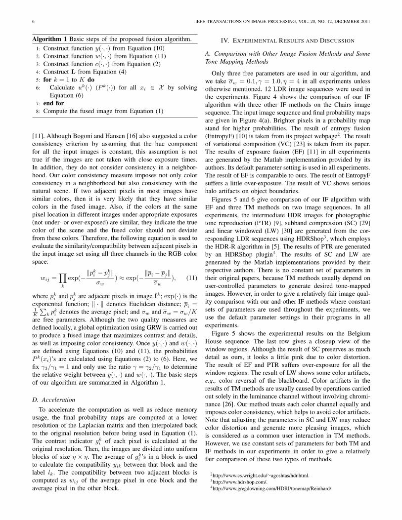
Only three free parameters are used in our algorithm, andwe take σw = 0.1, γ = 1.0, η = 4 in all experiments unlessotherwise mentioned. 12 LDR image sequences were used inthe experiments. Figure 4 shows the comparison of our IFalgorithm with three other IF methods on the Chairs imagesequence. The input image sequence and final probability mapsare given in Figure 4(a). Brighter pixels in a probability mapstand for higher probabilities. The result of entropy fusion(EntropyF) [10] is taken from its project webpage2. The resultof variational composition (VC) [23] is taken from its paper.The results of exposure fusion (EF) [11] in all experimentsare generated by the Matlab implementation provided by itsauthors. Its default parameter setting is used in all experiments.The result of EF is comparable to ours. The result of EntropyFsuffers a little over-exposure. The result of VC shows serioushalo artifacts on object boundaries.

Figures 5 and 6 give comparison of our IF algorithm withEF and three TM methods on two image sequences. In allexperiments, the intermediate HDR images for photographictone reproduction (PTR) [9], subband compression (SC) [29]and linear windowed (LW) [30] are generated from the cor-responding LDR sequences using HDRShop3, which employsthe HDR-R algorithm in [5]. The results of PTR are generatedby an HDRShop plugin4. The results of SC and LW aregenerated by the Matlab implementations provided by theirrespective authors. There is no constant set of parameters intheir original papers, because TM methods usually depend onuser-controlled parameters to generate desired tone-mappedimages. However, in order to give a relatively fair image qual-ity comparison with our and other IF methods where constantsets of parameters are used throughout the experiments, weuse the default parameter settings in their programs in allexperiments.

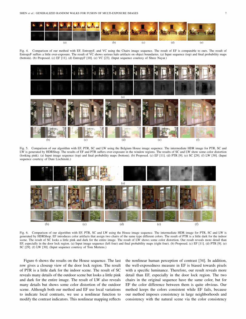
Figure 5 shows the experimental results on the BelgiumHouse sequence. The last row gives a closeup view of thewindow regions. Although the result of SC preserves as muchdetail as ours, it looks a little pink due to color distortion.The result of EF and PTR suffers over-exposure for all thewindow regions. The result of LW shows some color artifacts,e.g., color reversal of the blackboard. Color artifacts in theresults of TM methods are usually caused by operations carriedout solely in the luminance channel without involving chromi-nance [26]. Our method treats each color channel equally andimposes color consistency, which helps to avoid color artifacts.Note that adjusting the parameters in SC and LW may reducecolor distortion and generate more pleasing images, whichis considered as a common user interaction in TM methods.However, we use constant sets of parameters for both TM andIF methods in our experiments in order to give a relativelyfair comparison of these two types of methods.

2http://www.cs.wright.edu/∼agoshtas/hdr.html.3http://www.hdrshop.com/.4http://www.gregdowning.com/HDRI/tonemap/Reinhard/.

SHEN et al.: GENERALIZED RANDOM WALKS FOR FUSION OF MULTI-EXPOSURE IMAGES 7

(a) (b) (c) (d) (e)

Fig. 4. Comparison of our method with EF, EntropyF, and VC using the Chairs image sequence. The result of EF is comparable to ours. The result ofEntropyF suffers a little over-exposure. The result of VC shows serious halo artifacts on object boundaries. (a) Input sequence (top) and final probability maps(bottom). (b) Proposed. (c) EF [11]. (d) EntropyF [10]. (e) VC [23]. (Input sequence courtesy of Shree Nayar.)

(a)

(b) (c) (d) (e) (f)

Fig. 5. Comparison of our algorithm with EF, PTR, SC and LW using the Belgium House image sequence. The intermediate HDR image for PTR, SC andLW is generated by HDRShop. The results of EF and PTR suffers over-exposure in the window regions. The results of SC and LW show some color distortion(looking pink). (a) Input image sequence (top) and final probability maps (bottom). (b) Proposed. (c) EF [11]. (d) PTR [9]. (e) SC [29]. (f) LW [30]. (Inputsequence courtesy of Dani Lischinski.)

(a)

(b) (c) (d) (e) (f)

Fig. 6. Comparison of our algorithm with EF, PTR, SC and LW using the House image sequence. The intermediate HDR image for PTR, SC and LW isgenerated by HDRShop. EF introduces color artifacts that assign two chairs of the same type different colors. The result of PTR is a little dark for the indoorscene. The result of SC looks a little pink and dark for the entire image. The result of LW shows some color distortion. Our result reveals more detail thanEF, especially in the door lock region. (a) Input image sequence (left four) and final probability maps (right four). (b) Proposed. (c) EF [11]. (d) PTR [9]. (e)SC [29]. (f) LW [30]. (Input sequence courtesy of Tom Mertens.)

Figure 6 shows the results on the House sequence. The lastrow gives a closeup view of the door lock region. The resultof PTR is a little dark for the indoor scene. The result of SCreveals many details of the outdoor scene but looks a little pinkand dark for the entire image. The result of LW also revealsmany details but shows some color distortion of the outdoorscene. Although both our method and EF use local variationsto indicate local contrasts, we use a nonlinear function tomodify the contrast indicators. This nonlinear mapping reflects

the nonlinear human perception of contrast [34]. In addition,the well-exposedness measure in EF is biased towards pixelswith a specific luminance. Therefore, our result reveals moredetail than EF, especially in the door lock region. The twochairs in the original sequence have the same color, but forEF the color difference between them is quite obvious. Ourmethod keeps the colors consistent while EF fails, becauseour method imposes consistency in large neighborhoods andconsistency with the natural scene via the color consistency

8 IEEE TRANSACTIONS ON IMAGE PROCESSING, VOL. 20, NO. 12, DECEMBER 2011

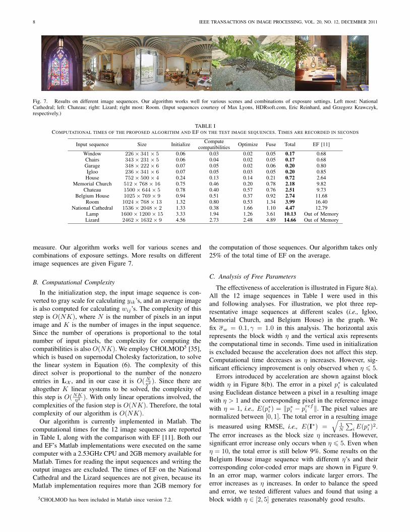
Fig. 7. Results on different image sequences. Our algorithm works well for various scenes and combinations of exposure settings. Left most: NationalCathedral; left: Chateau; right: Lizard; right most: Room. (Input sequences courtesy of Max Lyons, HDRsoft.com, Eric Reinhard, and Grzegorz Krawczyk,respectively.)

TABLE ICOMPUTATIONAL TIMES OF THE PROPOSED ALGORITHM AND EF ON THE TEST IMAGE SEQUENCES. TIMES ARE RECORDED IN SECONDS

Input sequence Size Initialize Compute Optimize Fuse Total EF [11]compatibilitiesWindow 226× 341× 5 0.06 0.03 0.02 0.05 0.17 0.68Chairs 343× 231× 5 0.06 0.04 0.02 0.05 0.17 0.68Garage 348× 222× 6 0.07 0.05 0.02 0.06 0.20 0.80Igloo 236× 341× 6 0.07 0.05 0.03 0.05 0.20 0.85House 752× 500× 4 0.24 0.13 0.14 0.21 0.72 2.64

Memorial Church 512× 768× 16 0.75 0.46 0.20 0.78 2.18 9.82Chateau 1500× 644× 5 0.78 0.40 0.57 0.76 2.51 9.73

Belgium House 1025× 769× 9 0.94 0.51 0.37 0.92 2.74 11.68Room 1024× 768× 13 1.32 0.80 0.53 1.34 3.99 16.40

National Cathedral 1536× 2048× 2 1.33 0.38 1.66 1.10 4.47 12.79Lamp 1600× 1200× 15 3.33 1.94 1.26 3.61 10.13 Out of MemoryLizard 2462× 1632× 9 4.56 2.73 2.48 4.89 14.66 Out of Memory

measure. Our algorithm works well for various scenes andcombinations of exposure settings. More results on differentimage sequences are given Figure 7.

B. Computational Complexity

In the initialization step, the input image sequence is con-verted to gray scale for calculating yik’s, and an average imageis also computed for calculating wij’s. The complexity of thisstep is O(NK), where N is the number of pixels in an inputimage and K is the number of images in the input sequence.Since the number of operations is proportional to the totalnumber of input pixels, the complexity for computing thecompatibilities is also O(NK). We employ CHOLMOD5 [35],which is based on supernodal Cholesky factorization, to solvethe linear system in Equation (6). The complexity of thisdirect solver is proportional to the number of the nonzeroentries in LX , and in our case it is O(Nη2 ). Since there arealtogether K linear systems to be solved, the complexity ofthis step is O(NKη2 ). With only linear operations involved, thecomplexities of the fusion step is O(NK). Therefore, the totalcomplexity of our algorithm is O(NK).

Our algorithm is currently implemented in Matlab. Thecomputational times for the 12 image sequences are reportedin Table I, along with the comparison with EF [11]. Both ourand EF’s Matlab implementations were executed on the samecomputer with a 2.53GHz CPU and 2GB memory available forMatlab. Times for reading the input sequences and writing theoutput images are excluded. The times of EF on the NationalCathedral and the Lizard sequences are not given, because itsMatlab implementation requires more than 2GB memory for

5CHOLMOD has been included in Matlab since version 7.2.

the computation of those sequences. Our algorithm takes only25% of the total time of EF on the average.

C. Analysis of Free Parameters

The effectiveness of acceleration is illustrated in Figure 8(a).All the 12 image sequences in Table I were used in thisand following analyses. For illustration, we plot three rep-resentative image sequences at different scales (i.e., Igloo,Memorial Church, and Belgium House) in the graph. Wefix σw = 0.1, γ = 1.0 in this analysis. The horizontal axisrepresents the block width η and the vertical axis representsthe computational time in seconds. Time used in initializationis excluded because the acceleration does not affect this step.Computational time decreases as η increases. However, sig-nificant efficiency improvement is only observed when η 6 5.

Errors introduced by acceleration are shown against blockwidth η in Figure 8(b). The error in a pixel p∗i is calculatedusing Euclidean distance between a pixel in a resulting imagewith η > 1 and the corresponding pixel in the reference imagewith η = 1, i.e., E(p∗i ) = ‖p∗i − p

refi ‖. The pixel values are

normalized between [0, 1]. The total error in a resulting imageis measured using RMSE, i.e., E(I∗) =

√1N

∑iE(p∗i )

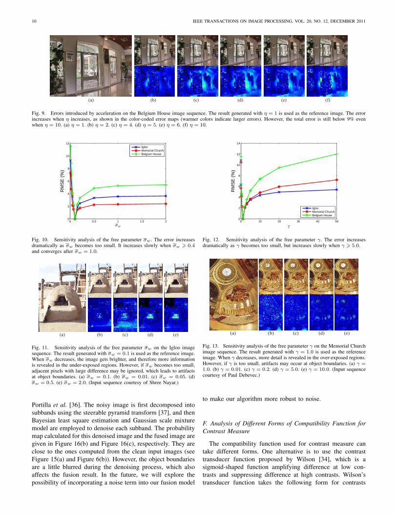
2.The error increases as the block size η increases. However,significant error increase only occurs when η 6 5. Even whenη = 10, the total error is still below 9%. Some results on theBelgium House image sequence with different η’s and theircorresponding color-coded error maps are shown in Figure 9.In an error map, warmer colors indicate larger errors. Theerror increases as η increases. In order to balance the speedand error, we tested different values and found that using ablock width η ∈ [2, 5] generates reasonably good results.

SHEN et al.: GENERALIZED RANDOM WALKS FOR FUSION OF MULTI-EXPOSURE IMAGES 9

(a)

(b)

1 2 3 4 5 6 7 8 9 10

1

2

3

4

5

6

7

8

9

10

11

12

13

14

15

Com

puta

tiona

l tim

e (s

ec)

IglooMemorial ChurchBelgium House

η

1 2 3 4 5 6 7 8 9 10

1

2

3

4

5

6

7

8

9

10

RM

SE

(%)

IglooMemorial ChurchBelgium House

η

Fig. 8. Analysis of acceleration with different block width η. Error is definedas the relative difference from the results generated with η = 1. Significantefficiency improvement is only observed when η 6 5 and significant errorincrease only occurs when η 6 5. (a) Effectiveness of acceleration. (b) Errorintroduced.

In the analysis of σw, we fix γ = 1.0, η = 4. The error isdefined similarly as in the analysis of η and the results withσw = 0.1 are used as reference images. The analysis on threerepresentative image sequences is plotted in Figure 10. Someresults on the Igloo sequence with different σw’s and theircorresponding color-coded error maps are shown in Figure 11.The error increases dramatically as σw becomes too small. Itincreases slowly when σw > 0.4 and converges after σw =1.0. When σw decreases, the image gets brighter, and thereforemore information is revealed in the under-exposed regions.However, if σw becomes too small, adjacent pixels with largedifference may be ignored, which leads to artifacts at objectboundaries. Therefore, we suggest using σw ∈ [0.05, 0.4].

In the analysis of γ, we fix σw = 0.1, η = 4. The error isdefined similarly as in the analysis of η and the results withγ = 1.0 are used as reference images. The analysis on threerepresentative image sequences is plotted in Figure 12. Someresults on the Memorial Church sequence with different γ’sand their corresponding color-coded error maps are shown inFigure 13. The error increases dramatically as γ becomes toosmall, but increases slowly when γ > 5.0. When γ decreases,more detail is revealed in the over-exposed regions. However,if γ is too small, like in the analysis of σw, artifacts may occurat object boundaries. Therefore, we suggest using γ ∈ [0.2, 5].

D. Post-Processing for Further Enhancement

Although our algorithm preserves more detail than EF, theresults of EF for some image sequences may have highercontrast (sharper) in certain regions. An example is given inFigure 14(a)(b). The tag near the bulb is clearly visible inour result but washed out in the result of EF. The region nearthe red book looks more colorful in the result of EF. Highercontrast can also be obtained from our method by applyinghistogram equalization as a post-processing step. In order toprovide a fair comparison, we added histogram equalizationto both methods. The images in Figure 14(c)(d) illustrate thatthe contrast in our result is improved while EF suffers a lossof detail during the process. Although histogram equalizationcauses our result to lose some information in the lamp region,our result still preserves more detail than the result of EF, e.g.,in the paper region.

E. Effect of Noise

One limitation of our algorithm is that it is sensitive tonoise in the input image sequence. One example is given inFigure 15. White Gaussian noise with 0 mean and variancefrom 0.001 to 0.01 with increments of 0.001 is added to oneof the four input images (pixel values are scaled to the range[0, 1]). For brevity, only the corrupted image with variance0.01 is shown in Figure 15, along with the original image. Inour algorithm, the initial probabilities are determined by localcontrast, and this local measure is sensitive to white Gaussiannoise because it is calculated by local variance. Since a globaloptimization scheme is used afterwards, the error caused bythe noise tends to propagate to a larger neighborhood. Thecolor-coded probability maps are given in Figure 15(a)(b),where warmer colors represent higher probabilities. Comparedto the probability map generated for the original image, higherprobabilities are assigned to pixels in the corrupted image,especially in the textureless regions like the walls. Even if weuse the correctly computed probability maps, pixels from thenoisy images still contribute to the fused image through the useof Equation (1). Therefore, the noisy images have significantinfluence on the fused images, as shown in Figure 15(c). Acloseup view of regions near the window is placed besideeach image to give a clearer view of the effect of noise.As the Gaussian noise variance increases, errors introducedby the noise become more obvious. However, the results byEF are also affected by the noise as shown in Figure 15(d).In addition, the noise in an input image also affects theHDR reconstruction process, which results in a noisy HDRimage. The tone mapping process fails to correct the noise inthis HDR image and the noise remains in the tone-mappedimage. PTR [9], SC [29], and LW [30] generate similarlyaffected results. Therefore, only the result of PTR is givenin Figure 15(e).

One solution to this problem is to add a pre-processing stepto reduce the noise in the input images. One example is givenin Figure 16. The input sequence is the House image sequence,where one image is corrupted with white Gaussian noise with 0mean and 0.01 variance as shown in Figure 15(b). Figure 16(a)gives the denoised image using the method proposed by

10 IEEE TRANSACTIONS ON IMAGE PROCESSING, VOL. 20, NO. 12, DECEMBER 2011

(a) (b) (c) (d) (e) (f)

Fig. 9. Errors introduced by acceleration on the Belgium House image sequence. The result generated with η = 1 is used as the reference image. The errorincreases when η increases, as shown in the color-coded error maps (warmer colors indicate larger errors). However, the total error is still below 9% evenwhen η = 10. (a) η = 1. (b) η = 2. (c) η = 4. (d) η = 5. (e) η = 6. (f) η = 10.

0 0.5 1 1.5 20

2

4

6

8

10

12

σw

RM

SE

(%)

IglooMemorial ChurchBelgium House

Fig. 10. Sensitivity analysis of the free parameter σw . The error increasesdramatically as σw becomes too small. It increases slowly when σw > 0.4and converges after σw = 1.0.

(a) (b) (c) (d) (e)

Fig. 11. Sensitivity analysis of the free parameter σw on the Igloo imagesequence. The result generated with σw = 0.1 is used as the reference image.When σw decreases, the image gets brighter, and therefore more informationis revealed in the under-exposed regions. However, if σw becomes too small,adjacent pixels with large difference may be ignored, which leads to artifactsat object boundaries. (a) σw = 0.1. (b) σw = 0.01. (c) σw = 0.05. (d)σw = 0.5. (e) σw = 2.0. (Input sequence courtesy of Shree Nayar.)

Portilla et al. [36]. The noisy image is first decomposed intosubbands using the steerable pyramid transform [37], and thenBayesian least square estimation and Gaussian scale mixturemodel are employed to denoise each subband. The probabilitymap calculated for this denoised image and the fused image aregiven in Figure 16(b) and Figure 16(c), respectively. They areclose to the ones computed from the clean input images (seeFigure 15(a) and Figure 6(b)). However, the object boundariesare a little blurred during the denoising process, which alsoaffects the fusion result. In the future, we will explore thepossibility of incorporating a noise term into our fusion model

0 10 20 30 40 500

2

4

6

8

10

12

14

R

MS

E (

%)

IglooMemorial ChurchBelgium House

Fig. 12. Sensitivity analysis of the free parameter γ. The error increasesdramatically as γ becomes too small, but increases slowly when γ > 5.0.

(a) (b) (c) (d) (e)

Fig. 13. Sensitivity analysis of the free parameter γ on the Memorial Churchimage sequence. The result generated with γ = 1.0 is used as the referenceimage. When γ decreases, more detail is revealed in the over-exposed regions.However, if γ is too small, artifacts may occur at object boundaries. (a) γ =1.0. (b) γ = 0.01. (c) γ = 0.2. (d) γ = 5.0. (e) γ = 10.0. (Input sequencecourtesy of Paul Debevec.)

to make our algorithm more robust to noise.

F. Analysis of Different Forms of Compatibility Function forContrast Measure

The compatibility function used for contrast measure cantake different forms. One alternative is to use the contrasttransducer function proposed by Wilson [34], which is asigmoid-shaped function amplifying difference at low con-trasts and suppressing difference at high contrasts. Wilson’stransducer function takes the following form for contrasts

SHEN et al.: GENERALIZED RANDOM WALKS FOR FUSION OF MULTI-EXPOSURE IMAGES 11

(a) (b) (c) (d)

Fig. 14. Comparison of our algorithm with EF [11] using the Lamp image sequence. The results of EF are generated on a smaller scale (1/4) of the inputsequence. Although the result of EF looks more colorful in some regions than our result, it preserves less detail. Especially for the lamp, the bulb and thetag beside it are clearly visible in our result but washed out in the result of EF. Although histogram equalization causes our result to lose some informationin the lamp region, our result still preserves more detail than the result of EF, e.g., in the paper region. (a) Proposed before histogram equalization. (b) EFbefore histogram equalization. (c) Proposed after histogram equalization. (d) EF after histogram equalization. (Input sequence courtesy of Martin Cadık.)

(a) (b)

(c) (d) (e)

Fig. 15. Analysis of our algorithm’s sensitivity to Gaussian white noise and comparison with other algorithms using the House image sequence. A closeupview of regions near the window is placed beside each image to give a clearer view of the effect of noise. As the Gaussian noise variance increases, errorsintroduced by the noise become more obvious. Our algorithm, EF, and PTR are all affected by the noise in the input image. (a) Original image (left) andits corresponding color-coded probability map (right) calculated by the proposed method (warmer colors represent higher probabilities). (b) Gaussian noise-corrupted image with 0 mean and 0.01 variance (left) and its corresponding color-coded probability map (right) calculated by the proposed method. (c) Fusedimage generated by the proposed method. (d) Fused image generated by EF [11]. (e) Tone-mapped image generated by PTR [9].

(a) (b) (c)

Fig. 16. Fusion result using our algorithm after adding a denoising step. The probability map calculated for this denoised image and the fused image areclose to the ones computed from the clean input images. However, the object boundaries are a little blurred during the denoising process, which also affectsthe fusion result. (a) Denoised image. (b) Color-coded probability map. (c) Fused image.

below or near the contrast threshold where |c|S = 1:

µ(c) =1

k(1 + (|c|S)Q)1/3 − 1

k, (12)

where c represents local contrast; k = 0.2599 is a parameterobtained by setting the contrast detection threshold to 0.75;Q = 3.0 is an empirically determined parameter; S is calledthe contrast sensitivity and in our experiment we set S =

10.75Cmax

, where Cmax represents the maximum magnitude ofthe local contrast detected from the input sequence. Becauseof this setting of S, all contrasts are below or near the

threshold. Therefore, Equation (12) is used in our experimentinstead of the unified transducer function in [34] that combinesEquation (12) and a function for high suprathreshold contrasts.In our experiment, the local contrast cki at the ith pixel in imageIk is calculated based on Weber contrast:

cki =4LkiLb

, (13)

where we take 4Lki as the luminance difference between thepixel pki and the average pixel of its 3× 3 neighborhood and

12 IEEE TRANSACTIONS ON IMAGE PROCESSING, VOL. 20, NO. 12, DECEMBER 2011

(a) (b) (c)

Fig. 17. Comparison between the results obtained from our current compat-ibility function (Equation (10)) and from Wilson’s transducer function withWeber contrast (Equations (12) and (13)) using the Memorial Church imagesequence. With all other parameter settings the same, Wilson’s transducerfunction with Weber contrast preserves more detail in the window regions,but produces contrast reversals at some places near the windows. When γis increased to 100 to give more emphasis on color consistency, the contrastreversals disappear although with some loss of detail. However, the brightnessof the entire fused image also decreases. (a) Equation (10) with σw = 0.1,γ = 1.0, and η = 4. (b) Equations (12) and (13) with σw = 0.1, γ = 1.0,and η = 4. (c) Equations (12) and (13) with σw = 0.1, γ = 100, and η = 4.

Lb as the average luminance of the input sequence. Lb canalso be taken as the local average luminance, but this maymake cki biased towards under-exposed pixels.

Figure 17 gives a comparison between the results obtainedby our current compatibility function (Equation (10)) andby Wilson’s transducer function coupled with Weber contrast(Equations (12) and (13)) using the Memorial Church imagesequence. With all other parameter settings the same, i.e.,σw = 0.1, γ = 1.0, and η = 4, Wilson’s transducer functionwith Weber contrast preserves more detail in the windowregions, but produces contrast reversals at some places near thewindows. These contrast reversals are caused by combiningpixels from input images with large exposure gaps. Whenγ is increased to give more emphasis on color consistency,the contrast reversals disappear although there is some loss ofdetail, as shown in Figure 17(c). However, the brightness ofthe entire fused image also decreases. The current form of thecompatibility function (Equation (10)) gives a better balancebetween local contrast and color consistency. We will analysecompatibility functions of other forms (e.g., [38]) and otherquality measures (e.g., [39]) that may enhance our algorithm’sperformance in the future.

V. CONCLUSIONS AND FUTURE WORK

In this paper, we proposed a new fusion algorithm for multi-exposure images considering fusion as a probabilistic compo-sition process. A generalized random walks framework wasproposed to compute the probabilities. Two quality measureswere considered: local contrast and color consistency. Unlikeprevious fusion methods, our algorithm achieves an optimalbalance between the two measures via a global optimization.Experimental results demonstrated that our probabilistic fu-sion produces good results, in which contrast is enhancedand details are preserved with high computational efficiency.

Compared to other fusion methods and tone mapping methods,our algorithm produces images with comparable or even betterqualities. In future work, we will explore more effectivequality measures and the possibility of incorporating multi-resolution technique in the fusion process to further enhanceour technique for different fusion problems. We will alsoexplore the possibility of applying the generalized randomwalks framework to other image processing problems.

ACKNOWLEDGMENT

The authors would like to thank Leo Grady for providingthe source code of the original random walks algorithm.The authors also would like to thank the reviewers for theirvaluable comments. The support of Killam Trusts, iCORE, andAlberta Advanced Education and Technology is also gratefullyacknowledged.

REFERENCES

[1] S. K. Nayar and T. Mitsunaga, “High dynamic range imaging: spatiallyvarying pixel exposures,” in Proc. IEEE Conf. Comput. Vis. PatternRecognit., vol. 1, 2000, pp. 472–479.

[2] H. Mannami, R. Sagawa, Y. Mukaigawa, T. Echigo, and Y. Yagi, “Highdynamic range camera using reflective liquid crystal,” in Proc. Int. Conf.Comput. Vis., 2007, pp. 1–8.

[3] J. Tumblin, A. Agrawal, and R. Raskar, “Why i want a gradient camera,”in Proc. IEEE Conf. Comput. Vis. Pattern Recognit., vol. 1, 2005, pp.103–110.

[4] H. Seetzen, W. Heidrich, W. Stuerzlinger, G. Ward, L. Whitehead,M. Trentacoste, A. Ghosh, and A. Vorozcovs, “High dynamic rangedisplay systems,” in Proc. ACM SIGGRAPH, 2004, pp. 760–768.

[5] P. E. Debevec and J. Malik, “Recovering high dynamic range radiancemaps from photographs,” in Proc. ACM SIGGRAPH, 1997, pp. 369–378.

[6] M. Aggarwal and N. Ahuja, “High dynamic range panoramic imaging,”in Proc. Int. Conf. Comput. Vis., 2001, pp. 2–9.

[7] E. Reinhard, G. Ward, S. Pattanaik, P. Debevec, W. Heidrich, andK. Myszkowski, High dynamic range imaging: Acquisition, display, andimage-based lighting, 2nd ed. Morgan Kaufmann, 2010.

[8] G. Krawczyk, K. Myszkowski, and H.-P. Seidel, “Lightness perceptionin tone reproduction for high dynamic range images,” Comput. Graph.Forum, vol. 24, no. 3, pp. 635–645, 2005.

[9] E. Reinhard, M. Stark, P. Shirley, and J. Ferwerda, “Photographic tonereproduction for digital images,” in Proc. ACM SIGGRAPH, 2002, pp.267–276.

[10] A. Goshtasby, “Fusion of multi-exposure images,” Image Vision Com-put., vol. 23, no. 6, pp. 611–618, 2005.

[11] T. Mertens, J. Kautz, and F. Van Reeth, “Exposure fusion,” in Proc.Pacific Graphics, 2007, pp. 382–390.

[12] M. Kumar and S. Dass, “A total variation-based algorithm for pixel-level image fusion,” IEEE Trans. Image Process., vol. 18, no. 9, pp.2137–2143, 2009.

[13] S. Zheng, W.-Z. Shi, J. Liu, G.-X. Zhu, and J.-W. Tian, “Multisourceimage fusion method using support value transform,” IEEE Trans. ImageProcess., vol. 16, no. 7, pp. 1831–1839, 2007.

[14] S. Li, J. T.-Y. Kwok, I. W.-H. Tsang, and Y. Wang, “Fusing images withdifferent focuses using support vector machines,” IEEE Trans. NeuralNetw., vol. 15, no. 6, pp. 1555–1561, 2004.

[15] H. Zhao, Q. Li, and H. Feng, “Multi-focus color image fusion in theHSI space using the sum-modified-laplacian and a coarse edge map,”Image Vision Comput., vol. 26, no. 9, pp. 1285–1295, 2008.

[16] L. Bogoni and M. Hansen, “Pattern-selective color image fusion,”Pattern Recogn., vol. 34, no. 8, pp. 1515–1526, 2001.

[17] G. Piella, “Image fusion for enhanced visualization: A variationalapproach,” Int. J. Comput. Vis., vol. 83, no. 1, pp. 1–11, 2009.

[18] V. S. Petrovic and C. S. Xydeas, “Gradient-based multiresolution imagefusion,” IEEE Trans. Image Process., vol. 13, no. 2, pp. 228–237, 2004.

[19] S. Z. Li, “Markov random field models in computer vision,” in Proc.European Conf. Comput. Vis., 1994, pp. 361–370.

[20] M. I. Smith and J. P. Heather, “A review of image fusion technology in2005,” in Proc. SPIE, vol. 5782, 2005, pp. 29–45.

SHEN et al.: GENERALIZED RANDOM WALKS FOR FUSION OF MULTI-EXPOSURE IMAGES 13

[21] I. Cheng and A. Basu, “Contrast enhancement from multiple panoramicimages,” in Proc. ICCV Workshop on OMNIVIS, 2007, pp. 1–7.

[22] W.-H. Cho and K.-S. Hong, “Extending dynamic range of two colorimages under different exposures,” in Proc. Int. Conf. Pattern Recogn.,vol. 4, 2004, pp. 853–856.

[23] S. Raman and S. Chaudhuri, “A matte-less, variational approach toautomatic scene compositing,” in Proc. Int. Conf. Comput. Vis., 2007,pp. 1–6.

[24] ——, “Bilateral filter based compositing for variable exposure photog-raphy,” in Proc. Eurographics Short Papers, 2009.

[25] M. Granados, B. Ajdin, M. Wand, C. Theobalt, H.-P. Seidel, and H. P. A.Lensch, “Optimal HDR reconstruction with linear digital cameras,” inProc. IEEE Conf. Comput. Vis. Pattern Recognit., 2010, pp. 215–222.

[26] M. Cadık, M. Wimmer, L. Neumann, and A. Artusi, “Evaluation of HDRtone mapping methods using essential perceptual attributes,” Comput.Graph., vol. 32, no. 3, pp. 330–349, 2008.

[27] G. W. Larson, H. Rushmeier, and C. Piatko, “A visibility matching tonereproduction operator for high dynamic range scenes,” IEEE Trans. Vis.Comput. Graph., vol. 3, no. 4, pp. 291–306, 1997.

[28] F. Drago, K. Myszkowski, T. Annen, and N. Chiba, “Adaptive loga-rithmic mapping for displaying high contrast scenes,” Comput. Graph.Forum, vol. 22, no. 3, pp. 419–426, 2003.

[29] Y. Li, L. Sharan, and E. H. Adelson, “Compressing and compandinghigh dynamic range images with subband architectures,” in Proc. ACMSIGGRAPH, 2005, pp. 836–844.

[30] Q. Shan, J. Jia, and M. S. Brown, “Globally optimized linear windowedtone mapping,” IEEE Trans. Vis. Comput. Graph., vol. 16, no. 4, pp.663–675, 2010.

[31] L. Grady, “Multilabel random walker image segmentation using priormodels,” in Proc. IEEE Conf. Comput. Vis. Pattern Recognit., vol. 1,2005, pp. 763–770.

[32] ——, “Random walks for image segmentation,” IEEE Trans. PatternAnal. Mach. Intell., vol. 28, no. 11, pp. 1768–1783, 2006.

[33] P. G. Doyle and J. L. Snell, Random walks and electric networks. MAA,1984.

[34] H. R. Wilson, “A transducer function for threshold and suprathresholdhuman vision,” Biological Cybernetics, vol. 38, no. 3, pp. 171–178,1980.

[35] Y. Chen, T. A. Davis, W. W. Hager, and S. Rajamanickam, “Algo-rithm 887: CHOLMOD, supernodal sparse Cholesky factorization andupdate/downdate,” ACM Trans. Math. Softw., vol. 35, no. 3, pp. 1–14,2008.

[36] J. Portilla, V. Strela, M. J. Wainwright, and E. P. Simoncelli, “Imagedenoising using scale mixtures of gaussians in the wavelet domain,”IEEE Trans. Image Process., vol. 12, no. 11, pp. 1338–1351, 2003.

[37] E. P. Simoncelli and W. T. Freeman, “The steerable pyramid: a flexiblearchitecture for multi-scale derivative computation,” in Proc. Int. Conf.Image Process., vol. 3, 1995, pp. 444–447.

[38] M. A. Garcıa-Perez and R. Alcala-Quintana, “The transducer model forcontrast detection and discrimination: formal relations, implications, andan empirical test,” Spatial Vision, vol. 20, no. 1-2, pp. 5–43, 2007.

[39] S. Winkler, “Vision models and quality metrics for image processingapplications,” Ph.D. dissertation, EPFL, 2000.