IEEE TRANSACTIONS ON CONTROL SYSTEMS TECHNOLOGY, VOL. 22, NO. 1, JANUARY 2014 1

Hierarchical Triple-Maglev Dual-RateControl Over a Profibus-DP Network

Ricardo Pizá, Julián Salt, Member, IEEE, Antonio Sala, Member, IEEE, and Ángel Cuenca, Member, IEEE

Abstract— This paper addresses a networked control systemapplication on an unstable triple-magnetic-levitation setup.A hierarchical dual-rate control using a Profibus-decentralizedperipherals network has been used to stabilize a triangularplatform composed of three maglevs. The difficulty in control isincreased by time-varying network-induced delays. To solve thisissue, a local decentralized H∞ control action is complementedby means of a lower rate output feedback controller on theremote side. Experimental results show good stabilization andreference position accuracy under disturbances.

Index Terms— Dual-rate control systems, linear matrixinequality, maglev, network delay, networked control systems,Profibus, stability analysis.

I. INTRODUCTION

WHEN a control application is projected on a network-based environment, in which different devices (sensor,

actuator, controller) are connected by means of a sharedcommunication medium [1]–[3], typical problems such asdata packet losses, lack of synchronization among devices,bandwidth limitations, and time-varying delays occur.

In some cases, the controlled process is very sensitive tothese problems. That is the case with a maglev-based platform[4], [5] in network-based control [6]. This magnetic levitationprocess control problem is challenging because each one ofthe systems that configure the platform are unstable and non-linear. Maglev platforms have also been used to demonstrateapplicability of control strategies in research literature [7], [8].

Also, magnetic levitation has a wide range of applica-tions [9], [10]. Thus, this paper demonstrates some network-based hierarchical control techniques in a three-maglevplatform.

Regarding the network to be selected in control, there areplenty of options with current technology. In an unstable fastsystem such as the one under consideration, a low-latencyhigh-bandwidth network would be a reasonable choice, for

Manuscript received October 24, 2011; revised July 30, 2012; acceptedSeptember 9, 2012. Manuscript received in final form October 2, 2012. Dateof publication November 12, 2012; date of current version December 17,2013. The work of R. Pizá, J. Salt, and Á. Cuenca was supported inpart by the Spanish Ministerio de Economía under Grant DPI2011-28507-C02-01, Grant DPI2009-14744-C03-03, and Grant ENE2010-21711-C02-01 and the Generalitat Valenciana Grant GV/2010/018. The work ofA. Sala was supported in part by the Spanish Ministerio de Economíaunder Grant DPI2011-27845-C02-01 and the Generalitat Valenciana GrantPROMETEO/2008/088. Recommended by Associate Editor C. De Persis.

The authors are with the Departamento de Ingeniería de Sistemas yAutomática, Instituto Universitario de Automática e Informática Indus-trial, Universitat Politecnica de Valencia, Valencia 46022, Spain (e-mail:rpiza@isa.upv.es; julian@isa.upv.es; asala@isa.upv.es; acuenca@isa.upv.es).

Color versions of one or more of the figures in this paper are availableonline at http://ieeexplore.ieee.org.

Digital Object Identifier 10.1109/TCST.2012.2222883

example, a network based on traditional field bus protocolssuch as Profibus, DeviceNet, CAN, InterBus, Field Bus, etc.,or a network based on newer industrial Ethernet protocols suchas ProfiNET, EtherNet/IP, Powerlink, EtherCAT, Modbus TCP,or SERCOS III [11]. Any of these networks may be suitablefor controlling this platform.

In this paper, a Profibus-decentralized peripherals (DP)with asynchronous operation mode has been selected [12].Some characteristics of Profibus make this network especiallyinteresting and challenging from a control engineering pointof view. There are two kinds of delays in this network: oneis the delay induced by data transfer between buffers andnodes; and the other one is the delay that appears in thetransmission between network nodes, whereby a distributionof time-varying communication delay appears. The chosencontrol strategy will also require a triggered bus mechanismfor synchronization based on Profibus freeze and sync com-mands. Other Profibus-based control applications are reportedin [13] and [14].

The objective of this paper is to experimentally demonstratea methodology, described below, for designing hierarchicalnetwork-based control systems for a multivariable unstableplant when computational capabilities and network band-width/sampling rates are restricted and data transfer delaysare present.

Therefore, a hierarchical control system is proposed here, asdepicted in Fig. 1. Indeed, due to the limitations in samplingrate and the communication delay magnitudes, it was notpossible to design a single stabilizing remote control in themaglev platform. Consequently, first of all, a fast-rate localdecentralized controller is designed and, in the followingstep, a more sophisticated slower rate “coordinating” remotecontrol is designed. Because of the lack of shared information,the decentralized controllers (which work perfectly with onemaglev) performed badly with the three-maglev platform inplace, falling frequently: neither the local-only nor the remote-only solutions were satisfactory.

For each maglev, a standalone local controller has beendesigned and implemented using robust H∞ control tech-niques [15]. The remote controllers have been designed usinglinear matrix inequality (LMI) gridding techniques [16].

The rest of this paper is organized as follows. Section IIdescribes the physical process (the triple-maglev system) usedas a test platform in the experiments. Section III (and anadditional appendix) presents how this process is modeledand linearized. The hierarchical control structure is introducedin Section IV. Before presenting the experimental results inSection VI, some network and hardware configuration aspects

1063-6536 © 2012 IEEE

2 IEEE TRANSACTIONS ON CONTROL SYSTEMS TECHNOLOGY, VOL. 22, NO. 1, JANUARY 2014

Fig. 1. Hierarchical control structure.

used in these experiments are detailed in Section V. Finally,Section VII concludes this paper.

II. THREE-MAGLEV PLATFORM DESCRIPTION

The experimental platform used in this paper comprisesseveral elements:

1) three magnetic levitation units. These units can be oper-ated in a standalone way, as done in experiment 1 inlater sections;

2) a Y-shaped levitated platform to which individualmaglevs can be attached;

3) a National Instruments CompactRio 9074 acting as alocal controller;

4) a desktop PC acting as a remote controller;5) a Profibus-DP network.

Let us now describe the most relevant characteristics ofthese elements.

The controlled plant is a levitated platform, shown in Fig. 2(left). This levitated platform has the shape of an equilateraltriangle with permanent magnets located at the corners of theplatform. A drawing scheme is shown in Fig. 3. The verticalposition of each magnet is controlled by an electromagnet.Thus, there are three maglevs located at the terminals of theplatform. Each maglev takes a voltage input signal to generatethe magnetic field and takes the vertical position measure usinga set of infrared sensor arrays.

The levitators have been provided by extra dimensiontechnologies (http://www.xdtech.com), model ML-EA.

Fig. 2. Experimental setup.

Fig. 3. Illustrations of the experimental setup.

1

23

X (alpha angle)

Y (beta angle)

Fig. 4. Platform dimensions (top and side view), reference model axis, andmaglev numeration.

The magnetic levitation unit includes its own levitator alongwith its power amplifier unit. The maglev provides positioninformation, from the infrared sensor array in ±10 V range.The control signal to be provided to the power amplifier mustbe also in ±10 V range.

In order to build the coupled platform, the three independentloads of the maglevs were attached to the above-referredY-shaped aluminum sheet. Fig. 4 shows a drawing with thelevitated structure. The dimensions are in millimeters, and inthe center of the platform the circular shapes correspond toan extra load (a 2-euro coin, 8.5 g) used in transient analy-sis experiments. The total weight for the levitated platformis 0.423 kg.

Further details on the model parameters relevant for controlare discussed in the Appendix.

A similar maglev platform can be found in other works,for example, in [17], as well as those based on predictive

PIZÁ et al.: HIERARCHICAL TRIPLE-MAGLEV DUAL-RATE CONTROL OVER A PROFIBUS-DP NETWORK 3

control [18], fuzzy control [19], [20], or some nonlinearcontrol methods [21].

III. MODELING AND LINEARIZATION

This section discusses how the specific model is obtainedand linearized in order to apply the control scheme proposedin later sections.

A. Single Maglev Modeling

The well-known Lagrange equations [22] can be used toderive the differential equations of electromechanical systems

d

dt

∂T

∂ q− ∂T

∂q+ ∂ D

∂ q+ ∂V

∂q= FG

where T , V , and D represent the generalized kinetic,1 poten-tial, and dissipation energies, respectively. FG denotes thegeneralized forces, and the variable q express one of thegeneralized coordinates.

Let us denote the air gap between the variable magnetand the levitated load with the variable z. Assuming infinitepermeability except at the air gap with permeability μ, anduniform magnetic flux density B , the energy Tmag stored inthe levitator’s air gap is

Tmag = B2

2μ· A · z

where A is the cross-sectional area and B given by Fμm/z,where Fm stands for the magnetomotive force [linear withcurrent N I (coil) plus a permanent magnet component I0, Nbeing the number of turns of the inductor]. In summary, themagnetic energy is

Tmag = (N I + I0)2μA

2z. (1)

The reader is referred to [23] (for instance) for details onmagnetic field modeling.

Adding the mechanical kinetic energy term Tmech =1/2mz2, the gravitational potential V = −mgz, the resistivedissipation R · i , and using both charge and air gap asgeneralized coordinates, the following nonlinear model canbe obtained (details omitted for brevity, see [24] for similarmodeling problems):

mz − μ(N I + I0)2 A

4z2 − mg = 0 (2)

μAN2

zI + μAN(I0 + N I )z

z2 + RI = V . (3)

Of course, the uniform-magnetic-field model is not exact,as there exist lateral and bottom air gaps. In addition, if theintensity polarity were abruptly changed, the flux lines forthe resulting magnetic field would be modified; however, weassume that such situations will not occur around the chosenoperation point.

1To avoid confusion, note that T will later denote sampling rate, butsymbolizing in this way kinetic energy keeps notation in this section similarto standard mechanics textbooks.

Equations (2) and (3), define the theoretical model. Assum-ing a suitable operating point, a linearized single maglevcontinuous-time model is obtained as

M

3· z(t) = f (t) (4)

f (t) = K1 I (t) + K2 · z(t) (5)

L I (t) + Q · z(t) + RI (t) = v(t) (6)

where M/3 is the mass of the whole levitated platformcorresponding to one levitator, f is the electromagnetic force,and the constants L, R, K1, and K2 are available in the levita-tor’s manual provided by the manufacturer. The parameter Qmodels the potential induced by the movement of the levitatedmagnet.2 The maglev’s numerical values for the parameterscan be found in Appendix.

Introducing a measurement equation

y(t) = K3 · z(t) (7)

the variable y is the position measurement taken with theinfrared sensor system, with K3 a linearized calibrationconstant available on the maglev user’s manual.

These equations can be expressed in state space form for ageneric maglev i as

⎛⎝

Ii (t)zi (t)zi (t)

⎞⎠ =

⎛⎜⎝

−RiLi

0 −Qi

Li

0 0 13K i

1M

3K i2

M 0

⎞⎟⎠ ·

⎛⎝

Ii (t)zi (t)zi (t)

⎞⎠ +

⎛⎝

1Li

00

⎞⎠ · vi (t)

yi (t) = (0 K i

3 0) ·

⎛⎝

Ii (t)zi (t)zi (t)

⎞⎠. (8)

B. Global Platform (Coupled) Model

When the global three-levitator platform is considered, itsposition will be determined by the height of the center ofmass and by two angular coordinates.3 Rigid-body dynamicequations must be then considered.

First of all, the meaning of z will be changed to denote thevertical displacement of the platform’s center of mass (zi willdenote each maglev’s). The linear motion is only consideredalong the z-axis

Mz =∑

i

fi .

Second, denoting the resulting torque vector as τ , the rotationof the platform around the center of gravity yields

J ω = τ − ω × (Jω)

2It has been estimated in a separate experiment by moving the maglev andmeasuring position and induced voltage (opening the circuit). A least squaresfit between a filtered numerical derivative of the position and the voltage hasbeen used (details omitted for brevity).

3The rest of the degrees of freedom, i.e., rotation around the vertical axisand two horizontal displacement coordinates, cannot be controlled with theavailable actuators. Fortunately, as the levitators are somehow attracted towardthe electromagnets also in the horizontal axis, these uncontrollable models arestable. Nevertheless they are only very lightly damped (by air, eddy currents,etc.; actually, damping is so subtle that it has not been considered in thecontrolled–vertical coordinate movement): the platform must be carefully andslowly positioned without introducing significant energy on these coordinates.

4 IEEE TRANSACTIONS ON CONTROL SYSTEMS TECHNOLOGY, VOL. 22, NO. 1, JANUARY 2014

where J is the inertia matrix. However, when linearizingaround zero rotational speed, and choosing small rotationsaround the principal axis (diagonal inertia matrix) as angularcoordinates, then the following equalities can be considered, αand β being the angles of rotation of levitated platform aroundX and Y axes, respectively:

Jx x α = τx (9)

Jyyβ = τy (10)

τx and τy being the torques on axis x and y, respectively, withthe chosen reference frame as shown in Fig. 4.

Expressions of torques at the center of gravity from each ofthe maglev electromagnetic forces are as follows:

τ1x = f1 L cos α, τ1y = 0

τ2x = f2 L cos α cos β sinπ

6, τ2y = f2 L cos α cos β sin

π

3

τ3x = f3 L cos α cos β sinπ

6, τ3y = f3 L cos α cos β sin

π

3

where L is the length of the arm, and α and β are the rotationangles around the x- and y-axis, respectively.

For sensor measurements, the expressions are as follows:

z1 = z + Lα

z2 = z − L sinπ

6· α + L sin

π

3· β

z3 = z + L sinπ

6· α − L sin

π

3· β.

Then, the equation of movement in the vertical directionis

Mz = f1 + f2 + f3.

The linearized torques around the horizontal position are

τ1x = f1 L, τ1y = 0

τ2x = f2 L sinπ

6, τ2y = f2 L sin

π

3

τ3x = f3 L sinπ

6, τ3y = f3 L sin

π

3.

Hence, the overall linearized system equations are asfollows:

L1 I1 + Q1 · z1 + R1 I1 = v1

L2 I2 + Q2 · z2 + R2 I2 = v2

L3 I3 + Q3 · z3 + R3 I3 = v3

f1 = K 11 I1 + K 1

2 z1 = K 11 I1 + K 1

2 Lα

f2 = K 21 I2 + K 2

2 z2 = K 21 I2 + K 2

2 L(

sinπ

3· β − sin

π

6· α

)

f3 = K 31 I3 + K 3

2 z3 = K 31 I3 + K 3

2 L(

sinπ

6· α − sin

π

3· β

)

Mz = f1 + f2 + f3

Jx x α = L(

f1 + f2 sinπ

6+ f3 sin

π

6

)

Jyyβ = L(

f2 sinπ

3+ f3 sin

π

3

).

Reorganizing, we get

I1 = − R1

L1I1 − Q1

L1z − Q1 L

L1α + 1

L1v1

I2 = − R2

L2I2 − Q2

L2z + Q2 L sin π

6

L2α − Q2 L sin π

3

L2β + 1

L2v2

I3 = − R3

L3I3 − Q3

L3z − Q3 L sin π

6

L3α + Q3 L sin π

3

L3β + 1

L3v3

z = K 11

MI1 + K 2

1

MI2 + K 3

1

MI3 + L(K 1

2 + sin π6 (K 3

2 − K 22 ))

Mα

+ L sin π3 (K 2

2 − K 32 )

Mβ

α = L K 11

Jx xI1 − L K 2

1

Jx xI2 − L K 3

1

Jx xI3

+ L2(K 12 + sin2 π

6 (K 22 − K 3

2 ))

Jx xα

+ L2 sin π6 sin π

3 (K 32 − K 2

2 )

Jx xβ

β = L K 21 sin π

3

JyyI2 + L K 3

1 sin π6

JyyI3

+ L2 sin π6 (K 3

2 sin π6 − K 2

2 sin π3 )

Jyyα

+ L2 sin π3 (K 2

2 sin π3 − K 3

2 sin π6 )

Jyyβ.

Therefore, denoting the state, input, and output vector as

x =

⎛⎜⎜⎜⎜⎜⎜⎜⎜⎜⎜⎜⎜⎝

I1I2I3zzααβ

β

⎞⎟⎟⎟⎟⎟⎟⎟⎟⎟⎟⎟⎟⎠

, u =⎛⎝

v1v2v3

⎞⎠ , y =

⎛⎝

K 13 z1

K 23 z2

K 33 z3,

⎞⎠ (11)

the state equations are

x = Ax + Bu (12)

y = Cx (13)

which are the system matrices in (14), shown at the bottomof next page.

IV. DISCRETE DUAL-RATE CLOSED-LOOP

MODELS AND CONTROL STRUCTURE

If the linear state equations (12) and (13) are discretized ata period T0 (with zero-order hold at the input), we get

x((k + 1)T0) = Ax(kT0) + Bu(kT0) (15)

y(kT0) = Cx(kT0) + Du(kT0). (16)

The state of each of the subsystems (to be used by eachdecentralized controller) will be denoted as xi in the sequel,and the output as yi . Obviously, the full state x above iscomposed by the juxtaposition of all xi and, due to the inertialcoupling, matrix A is not block-diagonal.

PIZÁ et al.: HIERARCHICAL TRIPLE-MAGLEV DUAL-RATE CONTROL OVER A PROFIBUS-DP NETWORK 5

+ v1 y1LOCALCONTROL 1

e1

r3

+

-

+ v2 y2e2

+ v3 y3e3

r2

r1

+

-

+

-

ri yi

LOCALCONTROL 2

LOCALCONTROL 3

MAGLEVPLATFORM

PROFIBUS-DP

REMOTECONTROLER

Fig. 5. Proposed hierarchical control system architecture, consistingof remote supervisory level controller, communications network, localcontrollers, and maglev platform.

Consider now the hierarchical control structure appearing inFig. 5. This structure depicts multiple controllers controllingin a decentralized way the above plant, and a remote controllerin charge of coordination.

Each subsystem has a one-degree-of-freedom local con-troller attached to it, whose state will be denoted as XCi , withequations given by

XCi((k + 1)T0) = A[i]d XCi(kT0) + B[i]

d ei (kT0) (17)

vi (K T0) = C [i]d XCi (kT0) + D[i]

d ei (kT0) (18)

where ei = ri − yi or, considering all of them in vectornotation, e = r − y.

Obviously, the overall controller state equations of the localsubsystem will have a block-diagonal structure: the notationXC will denote the state of all controllers (juxtaposingeach controller state in a larger vector). The state of the

A =

⎛⎜⎜⎜⎜⎜⎜⎜⎜⎜⎜⎜⎜⎜⎜⎜⎜⎝

− R1L1

0 0 0 − Q1L1

0 − Q1 LL1

0 0

0 − R2L2

0 0 0 − Q2L2

Q2 L sin π6

L20 − Q2 L sin π

3L2

0 0 − R3L3

0 0 − Q3L3

− Q3 L sin π6

L30

Q3 L sin π3

L3

0 0 0 0 1 0 0 0 0K 1

1M

K 21

MK 3

1M 0 0

L(K 12+sin π

6 (K 32−K 2

2 ))

M 0L sin π

3 (K 32 −K 2

2 )

M 00 0 0 0 0 0 1 0 0

L K 11

Jxx− L K 2

1Jxx

− L K 31

Jxx0 0

L2(K 12+sin2 π

6 (K 22 −K 3

2 ))

Jxx0

L2 sin π6 sin π

3 (K 32 −K 2

2 )

Jxx0

0 0 0 0 0 0 0 0 1

0L K 2

1 sin π3

Jyy

L K 31 sin π

6Jyy

0 0L2 sin π

6 (K 32 sin π

6 −K 22 sin π

3 )

Jyy0

L2 sin π3 (K 2

2 sin π3 −K 3

2 sin π6 )

Jyy0

⎞⎟⎟⎟⎟⎟⎟⎟⎟⎟⎟⎟⎟⎟⎟⎟⎟⎠

B =

⎛⎜⎜⎜⎜⎜⎜⎜⎜⎜⎜⎜⎜⎜⎝

1L1

0 00 1

L20

0 0 1L3

0 0 00 0 00 0 00 0 00 0 00 0 0

⎞⎟⎟⎟⎟⎟⎟⎟⎟⎟⎟⎟⎟⎟⎠

, C =⎛⎝

0 0 0 K 13 0 K 1

3 L 0 0 00 0 0 K 2

3 0 −K 23 L sin π

6 0 K 23 L sin π

3 00 0 0 K 3

3 0 K 33 L sin π

6 0 −K 33 L sin π

3 0

⎞⎠.

(14)

controlled system (three-maglev platform) plus that of thelocal controllers will be denoted as χ = (xT X T

C )T . Obviously,although the controller state equations are block-diagonal,there will be some coupling due to the plant not beingfully diagonal. The role of the remote controller will be tocompensate such coupling neglected in the local decentralizedside.

In order to achieve the coordination, the overall localsubsystem equations will be considered in the form

χ((k + 1)T0) = A0χ(kT0) + B0r(kT0) (19)

y(kT0) = C0χ(kT0) + D0r(kT0). (20)

A. Dual-Rate Modeling

The remote system will be in charge of controlling the localsubsystem over a network at a slower rate, because networklimitations will be assumed to exist, limiting the sampling rate(see Section V).

The local controllers will be operating at a fast samplingrate with period T0, and the remote controller at a slower rateT = NT0. The network-induced round-trip time delay betweena local controller sending yi and receiving ri will be denotedby di (kT ).

Some assumptions on the values of the delays in eachloop are needed. Ample detail will be given in Section V,but at this moment we may preliminarily assert that, due tothe chosen configuration of the Profibus communication, thesync and freeze commands will allow us to assume that thedelay is coincident in all channels and multiple of the localsampling period. In the sequel, such delay will be denoted byδ(kT ) = d(kT ) × T0. The value of d(kT ) will be assumedto be known at next sample time, given the sequence ofnetwork commands chosen for synchronization (see Section Vfor details).

6 IEEE TRANSACTIONS ON CONTROL SYSTEMS TECHNOLOGY, VOL. 22, NO. 1, JANUARY 2014

Fig. 6. Control and state update chronogram.

Although the hierarchical control structure is reminis-cent of a cascade control, conventional cascade-controldesign assumes a timescale separation so that a separate designis possible [25] and small delays would be negligible in theouter very low bandwidth loop. In the proposal here, theaction of the remote controller will be fast enough to influencethe stability and performance of the inner loop: bandwidthof both loops will be intentionally similar, and Lyapunovfunctions considering the whole remote+local+plant state willbe needed.

1) Slow-Rate Modeling: In order to design the remotecontroller, a slow-rate model (at period T = NT0) is needed.

Considering the fast-rate behavior (19), the slow-rate stateupdate equations will be given by the well-known convolutionexpression [26]

χ((k + 1)NT0) = AN0 χ(k NT0)

+N∑

h=1

Ah−10 B0r(((k + 1)N − h)T0). (21)

However, as the reference input is updated after a delay ofδ(kT ) = d(kT )T0 and kept constant until next update (seeFig. 6), the above must be corrected to

χ((k + 1)NT0) = AN0 χ(k NT0)+

⎛⎝AN−d(kT )

0

d(kT )∑j=1

A j−10 B0

⎞⎠

×r((k − 1)NT0) +⎛⎝

N−d(kT )∑i=1

Ai−10 B0

⎞⎠ r(k NT0)

= AN0 χ(k NT0) + B1(N, d(kT ))r((k − 1)NT0)

+B2(N, d(kT ))r(k NT0). (22)

By assumption, T will be strictly greater than d(kT )T0 ∀k,because the sampling period T has been selected in order toverify this restriction.4 If d(kT ) > N , the model would get

[e−2ϑT X X (A∗(N, d(kT )))T − MT (B∗(N, d(kT )))T

A∗(N, d(kT ))X − B∗(N, d(kT ))M X

]> 0 (26)

4For this purpose, some experimental offline tests have been done todetermine the maximum round-trip delay.

more complex, needing incorporation of further past values ofr , i.e., r((k − 2)NT0), etc. For simplicity, this issue will notbe pursued further.

If an augmented state �(kT ) = (χ(kT ), r((k − 1)T )′referred to the remote period T is considered, the system asseen by the upper level can be expressed as

�((k + 1)T ) =(

AN0 B1(N, d(kT ))

0 0

)�(kT )

+(

B2(N, d(kT ))I

)r(kT ). (23)

For brevity in further developments, notations A∗ and B∗are introduced in (23), yielding

�((k + 1)T ) = A∗(N, d(kT ))�(kT )

+B∗(N, d(kT ))r(kT ). (24)

The modeling procedure in Section III allows obtaining theabove matrices in the experimental platform.

B. Control Design Strategy

Having described the dual-rate modeling and notation, thissection discusses general ideas on the chosen control designmethodologies.

Basically, on one hand, three low-order (and hence with lowcomputational requirements) local controllers will be designedusing standard mixed-sensitivity H∞ control techniques [15],assuming a decoupled system.

On the other hand, LMI gridding and the nonstationaryKalman filter are used in the coordinating remote controller(in [16] and [27] for the basic formulae for the LMI-griddingapproach, and in [28] and [29] for the Kalman filter), assuminga fully coupled plant.

In this section, the control techniques in the remote side arereviewed for convenience. Note, importantly, that in order todevelop this control system structure, the delay d(kT ) must beknown. Conditions for applicability of a separation principleare also discussed in [16].

1) LMI Gridding: From the augmented model (24), thecontrol synthesis problem can be cast as a state-feedback one,leading to

r(kT ) = −F∗�(kT ). (25)

However, the gain F∗ must ensure robustness against theunknown round-trip delay d(kT ) because its value is notknown a priori at the time when r(kT ) is computed, its valuewill be later obtained by using the freeze/sync commands, butit will be useful only for the a posteriori observer part.

In order to achieve stabilizing controllers subject to time-varying delays, an LMI gridding procedure [16] is considered.From [16], there exist matrices X and M so that (26), shown

PIZÁ et al.: HIERARCHICAL TRIPLE-MAGLEV DUAL-RATE CONTROL OVER A PROFIBUS-DP NETWORK 7

Fig. 7. Coordination and synchronization chronogram (Profibus implementation of Figs. 5 and 6).

on the bottom of previous page is verified for any d(kT )which may arise in experimental operation: in this particularapplication, d(kT ) takes values in [1, . . . , N − 1].

If the LMIs are feasible, the feedback controllerF∗ = M X−1 stabilizes (24) with decay rate ϑ (continuous-time equivalent), and �(kT )T X−1�(kT ) is the associatedLyapunov function. As discussed in Section V, the experimen-tal setup required N = 4 and gridding on possible values ofd(kT ) = 1, 2, 3, so (26) is actually a collection of three LMIs.

2) Nonstationary Kalman Filter: Regarding the observerdesign for (24), as d(kT ) can be obtained from freeze/synccommands at the time when r((k +1)T ) is computed, Kalmangains depending on induced delays can be obtained withnonstationary Kalman filters [30], [31], whose equations areas follows:

P(kT ) = A∗(N, d(kT ))�(kT )A∗(N, d(kT ))T + V (kT )

(27)

L(kT ) = P(kT )CT (C P(kT )CT + W (kT ))−1 (28)

�((k + 1)T ) = (I − L(kT )C)P(kT ) (29)

where V (kT ) and W (kT ) are process and measurement noiseparameters. The observer gain is L(kT ), with an estimatedstate, denoted by �(kT ), obtained via the current-observerupdate equation

�(kT ) = (I − L(kT )C)

×(

A∗(N, d((k − 1)T )�((k − 1)T )

+ B∗(N, d((k − 1)T )r(kT )

)+ L(kT )y(kT ).

(30)

In order to implement the above equation, the packetreceived by the remote node should contain the array ofmeasurements y(kT ), the time in which they were measured,and the delay d((k − 1)T ) in the preceding cycle as explainedin the next section.

V. HARDWARE AND NETWORK CONFIGURATION

The control experiments developed in this paper have beenimplemented as follows.

In the first level, the local controllers have been imple-mented using a National Instruments CompactRIO device asshown in Fig. 2 (right).

The network was a Profibus-DP; its nodes were a ComSoftDFProfi-II DP card in the PC and a Profibus module cRioPB in the compactRio controller, the latter operating as abus master. Details on the network elements can be foundin http://www.comsoft.de and http://www.ni.com.

The available Profibus-DP bandwidth enables us to use asecond level where a remote coordinating control action isinjected at just every 20 ms. Indeed, the chosen Profibusconfiguration parameter was a bus rate of 187.5 kbits/s withasynchronous operation.

Let us now discuss how the remote control and local-level synchronization are carried out. Every T = 20 ms,the supervisor controller starts the control task as follows(symbolicaly depicted in Fig. 7).

1) Stage 1: Master node sends freeze command to slavenodes. All slaves receive the message at approximatelythe same time (with some microseconds jitter due tothe bus cycle) and freeze the inputs (from the process).In the next Profibus cycle, slaves send frozen inputs(measures) to master node. Receiving freeze commandis used also for synchronizing slave clocks to t = 1 ms.

2) Stage 2: Master node receives the measures from slavesand process data according to the control algorithm.

3) Stage 3: Master node sends sync command to slavenodes. Then, their outputs to the process are internallyupdated at the next Profibus cycle in the buffers but notapplied until an unsync command is received.

4) Stage 4: Master node sends the referred unsync com-mand to slaves, and then all of them update the outputs(reference to local controllers) simultaneously at the nextmultiple of the local sampling time T0. As the remotecontroller knows the moment in which it sent the unsynccommand, it can compute d(kT ) for the observer update.

5) Stage 5: With their internal sampling time T0 = 5 ms,local controllers perform the platform control algorithmwith no communication with the master node. At sam-pling time T = 20 ms, the measurements are taken andstored in the buffer. The master node starts again thecontrol process at t = 21 ms, and the sequence returnsto stage 1.

8 IEEE TRANSACTIONS ON CONTROL SYSTEMS TECHNOLOGY, VOL. 22, NO. 1, JANUARY 2014

TABLE I

DISTRIBUTION HISTOGRAM OF NETWORK ROUND-TRIP DELAY

Delay 5 ms 10 ms 15 ms

Occurrences 123 154 1 084 502 292 357

Percentage 8.21% 72.3% 19.49%

A. Distribution of Round-Trip Delays d(kT)

An experimental test was conducted to measure the magni-tude of the network-induced time delays: the most repeatedround-trip time delay corresponds to a 10-ms period, witheventual delays at 5 and 15 ms, as shown in Table I. Forthis reason, the grid of times for discretizing the system willbe formed by the set of values (5, 10, 15) ms.

VI. NUMERICAL RESULTS AND EXPERIMENTS

In this section, the numerical results of the controllercomputations and the experimental measurements will bedescribed.

Note that, although it is theoretically possible to control alinear system with a discrete-time controller at any desiredperiod, the disturbance rejection and tolerance to modelingerrors severely diminish as such period increases with unstablesystems. This fact is proved to be fundamental in our experi-ments, in the following sense.

1) The H∞ controllers designed for the long period T =20 ms were, in actual experiments, not able to stabilizeeven a single maglev in a local configuration with nonetwork delay, even though they were of course stablein the simulations. Hence, the slow-rate remote-onlycontrol option was not a viable solution.

2) On the other hand, a local controller at each of thelevitators with a SISO loop may be a viable solution.Indeed, local stabilizing controllers at T0 = 5 ms withthe decoupled model were obtained by H∞ techniques,and were able to stabilize appropriately a single maglev.

3) However, due to disregarded couplings, modeling erroris introduced which will degrade performance of thelocal-only decentralized controllers, as later experimentsshow. Of course, incorporating the coupling wouldrequire communication between the different subsys-tems, assumed to be feasible only via the chosen network(at a slower rate).

In summary, the above issues justify the need for theproposed dual-rate structure.

In order to deal with these issues, a set of experiments havebeen developed, as follows.

A. Preliminary Experiments: Single-Maglev Control

First of all, a preliminary experiment with a single maglev,not with the whole platform, has been developed. In this exper-iment, first, a standalone H∞ controller has been designed andimplemented. This type of controller is chosen in the localcontroller in order to suitably balance disturbance rejectionperformance versus tolerance to modeling errors at particularfrequencies.

Fig. 8. System’s sensitivity to additive uncertainty with different samplingrates.

A first set of controllers are designed for each single maglevusing a mixed-sensitivity approach using a set of weightvalues, i.e., sensitivity weight, control action weight, and com-plementary sensitivity weight. For the designed controllers,the values of these corresponding weights are 1, 0.2, and0.6. Using the robust toolbox MATLAB command [K, CL,GAM, INFO] = MIXSYN(G, 1, 0.2, 0.6), where G is theequivalent discrete model plant for state space maglev model,the different local controllers for each of the three maglevs areobtained. Weights have been chosen as constants to keep theresulting controller order low.

Experimentally, a set of controllers has been designed usingseveral sampling periods keeping the same design parameters.As a result of all the experiments, the greatest sampling periodthat could be satisfactorily used with the maglev was T0 =5 ms: with larger sampling periods, accumulated error canbecome too large, so it makes the one-maglev system unstableor on the verge of instability.

Fig. 8 shows the additive uncertainty sensitivity analysis,i.e., K/(1 + K G), when controller and plant (for a singlemaglev) are sampled at 5 and 20 ms. As the samplingtime increases, uncertainty in model and sensitivity increases,making the experimental system unstable.

As all the local controllers are very similar, the numericalvalue of just one of them is

G R(z) = u(z)

e(z)= 10.845(z + 1)(z − 0.878)(z − 0.641)

(z + 0.93)((z − 0.54)2 + 0.272).

(31)

An additional set of controllers is designed by adding an(approximate) integral term. Defining the continuous integratoras (G(τ s + 1)/Gτ s + 1), with a large enough G and a smallenough τ , this continuous term is discretized at T0 samplingtime using Tustin discretization method. This discretized termis included in the sensitivity weight (WI ) for calculatingthe new controller. In our case, the resulting weight was(WI (z) = (1.001z − 0.9982)/(z − 0.9997)). A new controlleris designed using this integrator term in the sensitivity weight(WI) [K, CL, GAM, INFO] = MIXSYN(G, WI, 0.2, 0.6). As a

PIZÁ et al.: HIERARCHICAL TRIPLE-MAGLEV DUAL-RATE CONTROL OVER A PROFIBUS-DP NETWORK 9

0 2 4 6 8 10 12 14 16 18−2.5

−2−1.5

−1−0.5

00.5

Time (s)

Pos

ition

err

or (

mm

)

0 2 4 6 8 10 12 14 16 18−0.5

00.5

11.5

22.5

3

Time (s)

Con

trol

sig

nal (

V)

Fig. 9. Single maglev experiment.

result, the new set of controllers is obtained. One of them is

G R(z) = 10.74(z + 1)(z − 0.99)(z − 0.88)(z − 0.71)

(z − 1)(z + 0.94)((z − 0.56)2 + 0.282)(32)

which, as expected, is very similar to (31) except at lowfrequencies.

With these numerical results, a first preliminary single-maglev experiment is developed, whose output appears inFig. 9. The experiment begins by activating the local controllerwithout the integrator [see (31)]. The system achieves anequilibrium point with position error, as expected, but thesystem performance is suitable. At time t = 10.5 s, thecontroller changes adding the integral term [see (32)] and, aftera 2-s transient, the system achieves the new equilibrium pointwith no position error. This experiment is performed with onlyone standalone maglev. After this experiment is concluded, theplatform is assembled with the tree maglevs, and the rest ofexperiments below are carried out.

In summary, this preliminary experiment demonstratesthat the chosen design parameters for the local controllersallow an adequate SISO control performance for the realplant.

B. Experiment 1: Three-Maglev Platform, No Network

This experiment is developed using the whole platformand the set of local controllers previously developed withoutintegral action (31). Therefore, the network and the supervisorlevel are not used yet. The experiment starts with platform atthe equilibrium point and, at time t = 2.5 s, a load change isapplied to the platform depositing a 2-euro coin in the centerof the triangular aluminum structure. As seen in Fig. 10, thesystem response seems to change to a new equilibrium point(i.e., position error) but it barely keeps there, and the platformbecomes unstable and drops at t = 5.5 s.

This is the result of coupling between the different maglevsin the whole platform system as single-maglev controllersworked perfectly when isolated.

0 2 4 6 8 10 12 14 16−1

−0.5

0

0.5

1

1.5

2

2.5

3

Time (s)

Pos

ition

err

or (

mm

)

Experiment 1Experiment 2

Fig. 10. Platform position in Experiments 1 and 2.

C. Experiment 2: Three-Maglev Platform, No Network,Integral Action

This experiment is the same as the previous one but usingcontrollers with the integral action included, as in (32). As inthe previous experiment, network and supervisor level are notused yet.

Although the integrator tries to recover the referenceposition, oscillations of increasing amplitude are generateddue to the load disturbance and, ultimately, the loop becomesunstable and the platform falls.

With these two experiments (Experiments 1 and 2), thecoupling in platform is demonstrated to be significant, and itmust be taken into account when designing the control system.

D. Experiment 3: Three-Maglev Platform, HierarchicalControl, No Integrator

This third experiment is developed using the network andan additional supervisor-level controller. Each maglev on theplatform keeps its own local controller (no integral action) aspreviously designed, i.e., the same set of controllers used asin Experiment 1, see (31).

At the higher level, in the remote side, a plant model isdeveloped following the results in previous sections, where theconsidered process is the set composed by the three maglevsystems and the corresponding local digital control subsystemswith period T0.

The resulting state feedback controller (25) obtained has again matrix of dimensions 3 × 21 as shown in Section (VI-E)depicted top on page 10.

This supervisor controller is implemented on remote side,jointly with the previously discussed observer.

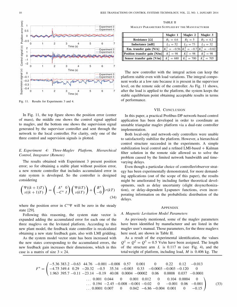
The experiment starts with platform at the equilibrium point,as shown in Fig. 11. At time t = 1.75 s, a load is applied, andafter a transient, the system acquires a new stable equilibriumpoint, but with position error (as expected). Compared toExperiment 1, now the supervisor control level compensatesfor the disturbances introduced by the coupling between thethree maglevs of the platform.

10 IEEE TRANSACTIONS ON CONTROL SYSTEMS TECHNOLOGY, VOL. 22, NO. 1, JANUARY 2014

0 1 2 3 4 5 6 7−0.5

0

0.5

1

Time (s)

Pos

ition

err

or (

mm

)

0 1 2 3 4 5 6 7−2−1012

Time (s)

Con

trol

sig

nal (

v)

0 1 2 3 4 5 6 7−0.4−0.3−0.2−0.1

0

Time (s)Sup

ervi

sion

sig

nal (

v)

Experiment 3Experiment 4

Experiment 3Experiment 4

Experiment 3Experiment 4

Fig. 11. Results for Experiments 3 and 4.

In Fig. 11, the top figure shows the position error (centerof mass), the middle one shows the control signal appliedto maglev, and the bottom one shows the supervision signalgenerated by the supervisor controller and sent through thenetwork to the local controller. For clarity, only one of thethree control and supervision signals is plotted.

E. Experiment 4: Three-Maglev Platform, HierarchicalControl, Integrator (Remote)

The results obtained with Experiment 3 present positionerror; so for obtaining a stable plant without position error,a new remote controller that includes accumulated error instate system is developed. So the controller is designedconsidering(

�((k + 1)T )s((k + 1)T )

)=

(A∗ 0

−C∗ I

) (�(kT )s(kT )

)+

(B∗−0

)r(kT )

(34)

where the position error in C∗� will be zero in the steadystate [29].

Following this reasoning, the system state vector isexpanded adding the accumulated error for each one of thethree maglevs on the levitated platform. According to thisnew plant model, the feedback state controller is recalculatedobtaining a new state feedback gain, also with LMI gridding.

As the system model vector state has been increased withthe new states corresponding to the accumulated errors, thenew feedback gain increases their dimensions, which in thiscase is a matrix of size 3 × 24.

F∗ =⎛⎝

−5.36 383.2 −0.63 44.76 −0.001 −0.008 0.57 0.001 0 0.22 0.12 −0.013−4.75 349.4 0.29 −20.32 −0.5 35.34 −0.003 0.33 −0.0003 −0.003 −0.120 01.963 395.7 −0.11 −23.14 −0.19 40.08 0.0004 −00002 0.06 0.0008 0.037 −0.0001

. . . 0.001 0.044 0 0.001 0.012 0 0.104 0.0004 0

. . . 0.194 −2.45 −0.008 −0.001 −0.02 0 −0.001 0.06 −0.001

. . . 0.0001 0.007 0 0.042 −6.86 −0.004 0.001 0 −0.15

⎞⎠ (33)

TABLE II

MAGLEV PARAMETERS SUPPLIED BY THE MANUFACTURER

Maglev 1 Maglev 2 Maglev 3

Resistance [ ] R1 = 4.6 R2 = 5 R3 = 4.2

Inductance [mH] L1 = 52 L2 = 73 L3 = 32

Em. transfer gain [N/A] K 11 = −0.56 K 2

1 = −0.7 K 31 = −0.82

Position transfer gain [N/m] K 12 = 98 K 2

2 = 98 K 32 = 98

Sensor transfer gain [V/m] K 13 = 680 K 2

3 = 700 K 33 = 705

The new controller with the integral action can keep theplatform stable even with load variations. The integral compo-nent works at a low rate because it is present in the supervisorlevel, on the remote side of the controller. As Fig. 11 shows,after the load is applied to the platform, the system keeps thestable equilibrium point obtaining acceptable results in termsof performance.

VII. CONCLUSION

In this paper, a practical Profibus-DP network-based controlapplication has been developed in order to coordinate anunstable triangular maglev platform via a dual-rate controllerimplementation.

Both local-only and network-only controllers were unableto satisfactorily stabilize the platform. However, a hierarchicalcontrol structure succeeded in the experiments. A simplestabilization local control and a refined LMI-based + Kalmanfilter solution in the remote side allowed us to solve theproblem caused by the limited network bandwidth and time-varying delays.

Even though a particular choice of controller/observer strat-egy has been experimentally demonstrated, for more demand-ing applications (out of the scope of this paper), the resultsmight be ameliorated by including further theoretical devel-opments, such as delay uncertainty (slight desyncrhoniza-tion), or delay-dependent Lyapunov functions, even incor-porating information on the probabilistic distribution of thedelays.

APPENDIX

A. Magnetic Levitation Model Parameters

As previously mentioned, some of the maglev parametershave been identified by manufacturer and are listed in themaglev user’s manual. Those parameters, for the three maglevshere used, are shown in Table II.

As a result of the experimental identification, the valuesQ1 = Q2 = Q3 = 0.5 Vs/m have been assigned. The lengthof the structure arm L is 0.117 m (see Fig. 4), and thetotal weight of platform, including load, M is 0.406 kg. The

PIZÁ et al.: HIERARCHICAL TRIPLE-MAGLEV DUAL-RATE CONTROL OVER A PROFIBUS-DP NETWORK 11

inertia matrix⎛⎝

Jx x Jxy Jxz

Jyx Jyy Jyz

Jzx Jzy Jzz

⎞⎠ =

⎛⎝

0.00293 0 00 0.00293 00 0 0.00541

⎞⎠

has been obtained via CAD software (modeling the object withsolid geometry, assigning the weights and obtaining inertialdata from the CAD analysis module).

Noise matrices used in Kalman filter, V and W , are diagonalmatrices with values of 0.0062 and 0.01, respectively. Mea-surement noise W is deduced by obtaining sensor measureswith the still platform, mechanically fixed. The variationsmeasured about mean value correspond to noise and thisvalue is used for characterizing the matrix. V characterizesinput noises and modeling errors, and it has been adjustedexperimentally to obtain suitable observer dynamics.

REFERENCES

[1] Y. Tipsuwan and M. Chow, “Control methodologies in networkedcontrol systems,” Control Eng. Pract., vol. 11, no. 10, pp. 1099–1111,2003.

[2] Y. Halevi and A. Ray, “Integrated communication and control systems.I-Analysis,” ASME, Trans. J. Dynamic Syst., Meas. Control, vol. 110,pp. 367–373, Dec. 1988.

[3] T. Yang, “Networked control system: A brief survey,” IEE Proc.-ControlTheory Appl., vol. 153, no. 4, pp. 403–412, Jul. 2006.

[4] S. Banerjee, D. Prasad, and J. Pal, “Design, implementation, and testingof a single axis levitation system for the suspension of a platform,” ISATrans., vol. 46, no. 2, pp. 239–246, Apr. 2007.

[5] W. Kim, S. Verma, and H. Shakir, “Design and precision constructionof novel magnetic-levitation-based multi-axis nanoscale positioning sys-tems,” Precis. Eng., vol. 31, no. 4, pp. 337–350, 2007.

[6] W. Kim, K. Ji, and A. Ambike, “Real-time operating environment fornetworked control systems,” IEEE Trans. Autom. Sci. Eng., vol. 3, no. 3,pp. 287–296, Jul. 2006.

[7] J. Paddison, H. Ohsaki, and E. Masada, “Control strategies for Maglevelectromagnetic suspension bogies,” in Proc. 35th IEEE Decision Con-trol, vol. 3. Dec. 1996, pp. 2796–2797.

[8] R.-J. Wai and J.-D. Lee, “Performance comparisons of model-free control strategies for hybrid magnetic levitation system,” IEEProc.-Electr. Power Appl., vol. 152, no. 6, pp. 1556–1564, Nov.2005.

[9] P. Holmer, “Faster than a speeding bullet train,” IEEE Spectrum, vol. 40,no. 8, pp. 30–34, Aug. 2003.

[10] P. Berkelman and M. Dzadovsky, “Large motion range magnet levitationusing a planar array of coils,” in Proc. IEEE Int. Conf. Robot. Autom.,May 2009, pp. 3950–3951.

[11] D. Hristu-Varsakelis and W. S. Levine, Handbook of Networked andEmbedded Control Systems. Boston, MA: Birkhäuser, 2008.

[12] K. Lee, S. Lee, and M. Lee, “Remote fuzzy logic control of networkedcontrol system via Profibus-DP,” IEEE Trans. Ind. Electron., vol. 50,no. 4, pp. 784–792, Aug. 2003.

[13] Z. Lie-Ping, Z. Yun-Sheng, and Z. Qun-Ying, “Remote control based onOPC and Profibus-DP bus,” Control Eng. China, vol. 5, pp. 594–597,May 2008.

[14] V. Casanova, J. Salt, A. Cuenca, and V. Mascarós, “Networked controlsystems over Profibus-DP: Simulation model,” in Proc. IEEE Int. Conf.Control Appl., Oct. 2006, pp. 1337–1342.

[15] K. Zhou, Essentials of Robust Control. Englewood Cliffs, NJ: Prentice-Hall, 1998.

[16] A. Sala, “Computer control under time-varying sampling period: AnLMI gridding approach,” Automatica, vol. 41, no. 12, pp. 2077–2082,Dec. 2005.

[17] C. Fernández, M. Vicente, and L. Jiménez, “Virtual laboratories forcontrol education: A combined methodology,” Int. J. Eng., vol. 21, no. 6,pp. 1059–1067, 2005.

[18] R. Fama, R. Lopes, A. Milhan, R. Galvão, and B. Lastra, “Predictivecontrol of a magnetic levitation system with explicit treatment ofoperational constraints,” in Proc. 18th Int. Congr. Mech. Eng., OuroPreto, MG, 2005, pp. 1–8.

[19] K. Erkan and T. Koseki, “Fuzzy model-based monlinear Maglev controlfor active vibration control systems,” Int. J. Appl. Electromagn. Mech.,vol. 25, no. 1, pp. 543–548, 2007.

[20] H. Han-Hui and T. Qing, “Decoupling fuzzy PID control for magneticsuspended table,” J. Central South Univ. Sci. Technol., vol. 4, pp. 963–968, Apr. 2009.

[21] N. Al-Muthairi and M. Zribi, “Sliding mode control of a magneticlevitation system,” Math. Probl. Eng., vol. 2, no. 2004, pp. 93–107,2004.

[22] J. E. Marsden and J. Scheurle, “The reduced Euler-Lagrange equations,”in Proc. Fields Instrum. Commun., 1992, pp. 139–164.

[23] J. Van Bladel, Electromagnetics Fields. New York: Wiley, 1964.[24] A. El Hajjaji and M. Ouladsine, “Modeling and nonlinear control of

magnetic levitation systems,” IEEE Trans. Ind. Electron., vol. 48, no. 4,pp. 831–838, Aug. 2001.

[25] K. Ogata, Modern Control Engineering. Englewood Cliffs, NJ: Prentice-Hall, 2010.

[26] P. Albertos, “Block multirate input-output model for sampled-datacontrol systems,” IEEE Trans. Autom. Control, vol. 35, no. 9, pp. 1085–1088, Sep. 1990.

[27] A. Sala, “Improving performance under sampling-rate variations viageneralized hold functions,” IEEE Trans. Control Syst. Technol., vol. 15,no. 4, pp. 794–797, Jul. 2007.

[28] R. F. Stengel, Optimal Control and Estimation. New York: Dover, 1994.[29] A. Sala, Multivariable Control Systems: An Engineering Approach. New

York: Springer-Verlag, 2004.[30] J. Tornero, R. Pizá, P. Albertos, and J. Salt, “Multirate LQG controller

applied to self-location and path-tracking in mobile robots,” in Proc.IEEE/RSJ Int. Conf. Intell. Robots Syst., vol. 2. Aug. 2001, pp. 625–630.

[31] M. Mora, R. Pizá, and J. Tornero, “Multirate obstacle tracking and pathplanning for intelligent vehicles,” in Proc. IEEE Intell. Veh. Symp., Jun.2007, pp. 172–177.

Ricardo Pizá received the B.Eng. and Ph.D. degreesin control engineering from Valencia Technical Uni-versity, Valencia, Spain, in 1997 and 2003, respec-tively.

He is currently an Assistant Professor with theUniversitat Politècnica de València, Valencia. Hehas authored or co-authored several papers in jour-nals and conferences, and has been involved inseveral research projects funded by local indus-tries and government. His current research interestsinclude network-based control systems, computer-

aided manufacturing, and robotics.

Julián Salt (M’07) received the M.Sc. degree inindustrial engineering and the Ph.D. degree in con-trol engineering from the Technical University ofValencia, Valencia, Spain, in 1986 and 1992, respec-tively.

He is a Full Professor with the Technical Univer-sity of Valencia, where he is currently the Head ofthe Department of Systems Engineering and Control.He has been a supervisor of nine Ph.D. theses.He has co-authored over 70 papers in journals andconferences. His current research interests include

nonconventionally sampled control and networked control systems.

12 IEEE TRANSACTIONS ON CONTROL SYSTEMS TECHNOLOGY, VOL. 22, NO. 1, JANUARY 2014

Antonio Sala (M’03) was born in Valencia, Spain,in 1968. He received the B.Eng. degree (Hons.)in combined engineering from Coventry University,Coventry, U.K., in 1990, and the M.Sc. degree inelectrical engineering and the Ph.D. degree in con-trol engineering from Valencia Technical University,Valencia, in 1993 and 1998, respectively.

He has been with the Universitat Politecnica deValencia, Valencia, since 1993, where he is currentlya Full Professor and the Vice-Head of the Systemsand Control Engineering Department. He has super-

vised five Ph.D. theses and more than 25 final M.Sc. projects. He has beeninvolved in several research and mobility projects funded by local industries,government, and European community. He has authored or co-authored morethan 40 journal papers (25 works with more than 10 cites, H-index is 18).

Dr. Sala has been member of the IFAC Publications Committee for eightyears. He is an Associate Editor of the IEEE TRANSACTIONS ON FUZZY

SYSTEMS.

Ángel Cuenca (M’06) received the M.Eng. degreein computer engineering and the Ph.D. degree incontrol engineering from the Technical Universityof Valencia, Valencia, Spain, in 1998 and 2004,respectively.

He has been with the Department of SystemsEngineering and Control, Technical University ofValencia, since 2000, where he is currently an Asso-ciate Professor. He has been involved in severalresearch projects funded by Spanish government,and European community. He has authored or co-

authored over 40 journal and conference papers. His current research interestsinclude multirate control systems, networked control systems, and event-basedcontrol systems.