IEEE TPAMI REVISED MANUSCRIPT JUNE 2014 1 … · IEEE TPAMI REVISED MANUSCRIPT JUNE 2014 1...

IEEE TPAMI REVISED MANUSCRIPT JUNE 2014 1

Skeletonization and partitioning of digital imagesusing discrete Morse theoryOlaf Delgado-Friedrichs, Vanessa Robins, Adrian Sheppard

Abstract—We show how discrete Morse theory provides a rigorous and unifying foundation for defining skeletons and partitions ofgreyscale digital images. We model a greyscale image as a cubical complex with a real-valued function defined on its vertices (thevoxel values). This function is extended to a discrete gradient vector field using the algorithm presented in Robins, Wood, SheppardTPAMI 33:1646 (2011). In the current paper we define basins (the building blocks of a partition) and segments of the skeleton usingthe stable and unstable sets associated with critical cells. The natural connection between Morse theory and homology allows us toprove the topological validity of these constructions; for example, that the skeleton is homotopic to the initial object. We simplify thebasins and skeletons via Morse-theoretic cancellation of critical cells in the discrete gradient vector field using a strategy informed bypersistent homology. Simple working Python code for our algorithms for efficient vector field traversal is included. Example data aretaken from micro-CT images of porous materials, an application area where accurate topological models of pore connectivity are vitalfor fluid-flow modelling.

Index Terms—curve skeleton, surface skeleton, medial axis transform, watershed transform, discrete Morse theory, persistenthomology.

F

1 INTRODUCTION

S KELETONIZATION and partitioning operations arewell established approaches to summarising shapes

in digital image analysis. The skeleton of a shape is alower-dimensional object that retains essential aspectsof the shape’s topology and geometry, typically via acentred curve but it may also incorporate medial surfacepatches [1]. Partitioning, or shape decomposition, refersto the identification of simple regions that divide theshape into meaningful parts [2], [3]. Many researchershave observed the interrelation between the two con-structions; intuitively the skeleton describes how theregions of the partition are joined together. Despite thiscorrespondence, the two operations are usually treatedas completely separate computations, although somerecent work has started to combine the two [4]. In thispaper we define skeletonization and partitioning oper-ations for digital images based on a single constructionfrom discrete Morse theory.

Morse theory connects the topology of the sub-levelsets of a real-valued function to its critical points [5].With digital images the real-valued function, f , might bethe intensity values of a greyscale image or a distancefunction derived from a binarized image and the sub-level set consists of all voxels x where f(x) ≤ c. Therelevant definitions are given in Section 2. The Morsepartition defined in this paper is based on stable basinssurrounding local minima and is closely related to thewatershed transform. The Morse skeleton is built from

• All authors are at the Department of Applied Mathematics, ResearchSchool of Physics and Engineering, The Australian National University,Canberra ACT 0200.E-mail: [email protected]

paths between critical points and generalises construc-tions such as the contour or component tree (also calledthe Reeb graph), and the medial axis. Both are definedhere via a discrete vector field derived from a digitalimage using the algorithm described in [6]. As in thatpaper, the machinery of discrete Morse theory [7] allowsus to prove the topological validity of our constructions.These constructions are described in Section 3.

Any practical algorithm for image analysis must in-corporate a method for removing the artefacts of noise;in greyscale images this manifests as extraneous localextrema. A further advantage of Morse theory is that ithas a built-in technique for cancelling pairs of criticalpoints. We exploit this and the theory of persistenthomology to simplify the Morse skeleton and partitionsimultaneously in a way that preserves the most impor-tant structural features of an image. This is described inSection 4.

We have implemented efficient serial and parallelalgorithms for constructing, traversing and simplifyingthe discrete gradient vector field in C++ and provideworking Python code for some of the essential routinesin Section 5. The code is applied to some reference 3Dimages, and some micro-CT images of porous rocks.

1.1 Related work

There is a vast literature on the subject of skeletonizationfor shape analysis spread across a number of applicationdomains, and a comprehensive review is beyond thescope of this paper. A broad overview may be foundin the book by Siddiqi and Pizer [1], and a comparativesurvey of various algorithms in [8]. Typically, a skeletonis a lower-dimensional object that is homotopic to the

This is the author's version of an article that has been published in this journal. Changes were made to this version by the publisher prior to publication.The final version of record is available at http://dx.doi.org/10.1109/TPAMI.2014.2346172

Copyright (c) 2014 IEEE. Personal use is permitted. For any other purposes, permission must be obtained from the IEEE by emailing [email protected].


initial shape, centred with respect to the shape’s bound-ary; some definitions have an associated function thatreconstructs the original shape. The basic concept hasits roots in the 1967 paper by Blum where the skeletonor medial axis is imagined as the set of corner pointsgenerated as a front propagates from the boundary ofa 2d shape [9]. In current applications the initial datamay be binary or greyscale, 2D, 3D or 4D digital images,surface meshes, or unstructured point clouds [1]. Algo-rithms for constructing a skeleton from data are based onfinding singularities and ridges in distance or potentialfunctions, thinning by boundary propagation, or geo-metric methods including Voronoi diagrams [8], [10]. Fordigital images in particular, topology-preserving thin-ning by removing simple points is a popular techniquewith the most successful implementations often usingdistance or potential functions to direct the removal ofvoxels, see [11] for a recent example. The discrete Morse-theoretic skeleton defined in this paper is closely relatedto all of these approaches and provides a theoreticalframework for unifying thinning and ridge-finding al-gorithms.

Discrete Morse theory also provides a framework forpartitioning, or shape decomposition, that is closely re-lated to the watershed transform [2], [12]. The connectionbetween watersheds and Morse theory has long beenrecognized, both concepts are traced back to a paper byMaxwell [13]. Applications of Morse theory to shape andimage analysis are covered in the 2008 review article [14].

Connections between Morse theory and persistenthomology in the context of data and image analysiswere first explored in [15], which stimulated a significantstream of research in scientific visualization of two- andthree-dimensional data. For example, in [16] a Morse-theoretic approach to segmentation with simplificationinformed by persistent homology is implemented usingsimplicial piece-wise linear approximations to grey-scaleimages. Earlier (non-persistent) homology computationsfrom image data are found in [17]. In the past five yearsthe use of discrete Morse theory in digital image analysishas received increasing attention [6], [18], [19], [20], [21].

Recent applications of persistent homology to charac-terise three-dimensional structure of interest to physicistsinclude the distribution of galaxies in the universe [22],[23], and porous or granular materials [24], [25], [26].

1.2 Contributions of this paper

This paper contributes a theoretical understanding,based on discrete Morse theory, for skeletonization andwatershed transform operations in digital image anal-ysis. It provides a definition of the Morse skeleton asthe union of unstable complexes of critical cells and aproof that the Morse skeleton is homotopic to the initialcomplex. The stable basin of a minimum is defined, andit is shown that the basins of all local minima parti-tion the image. The relationship between adjacencies ofcritical points in the Morse skeleton and adjacencies of

the basins is clarified by introducing the concept of abridge. The final theoretical contribution is to elucidateconnections between simplification of the discrete Morsevector field and the persistent homology of the sequenceof level subcomplexes, in a similar vein to work in [19],[27]. Alongside the theory, efficient serial algorithms arepresented for the essential tasks of traversing the discretevector field and determining paths between critical cells;Python and C++ implementations are available from theauthors.

2 PREREQUISITES

2.1 Digital images as cubical complexesA three-dimensional greyscale digital image can be mod-elled by a function g : D → R, where D ⊂ Z3 is typicallya rectangular subset of the discrete lattice:

D = {(i, j, k) ∈ Z3 | 0 ≤ i ≤ I, 0 ≤ j ≤ J, 0 ≤ k ≤ K}.

A point x ∈ D is called a voxel (or pixel in two dimen-sions).

Following Kovalevsky [28], we model digital imagesby cubical complexes. In our setting, the voxels (i, j, k) ∈D are the vertices (0-cells) of the complex. Higher-dimensional cells are the unit edges (1-cells) betweenvoxels whose coordinates differ by one in a single axis,unit squares (2-cells), and unit cubes (3-cells). We writeK for the collection of all such p-cells built from voxelsin D with p = 0, 1, 2, 3. We often denote the dimensionof a cell by a superscript: α(p). A cell α(p) ∈ K is a faceof another cell β(q) if p < q and the vertices of α are asubset of the vertices of β. If this is the case then wewrite α(p) < β(q). We can also say that β is a coface of α.If α(p) < β(q) with q = p+1, we call α a facet of β and βa cofacet of α. A set of such cells S is a complex if for anyα ∈ S, all its faces are also in S. The set K is a complex,and a complex X ⊂ K is called a subcomplex of K.

We initially extend the greyscale function g to the fullcubical complex K by taking the maximal value from thevertices of a cell:

g(β) := max{g(α) | α(0) < β,α ∈ D}.

Given any function defined on a complex f : K → R wecan study the subcomplexes derived from the level cutson f ,

Kf (c) := {α | α ≤ β for f(β) ≤ c}.

This is called the level subcomplex at value c with respectto f . For the greyscale image function g extended tothe cubical complex as above, these level subcomplexesare simply Kg(c) = {β | g(β) ≤ c}. The connectivity ofthe cubical level subcomplex with voxels as vertices isequivalent to using the standard 6-neighbourhood of 3Ddigital topology: voxel (i, j, k) is connected to a voxelon a face diagonal, say (i + 1, j + 1, k), if and only ifat least one of the voxels (i + 1, j, k) and (i, j + 1, k)is present. However, as will be seen below, extendingthe image to a complex in this way allows us to apply




a number of sophisticated theoretical tools, particularlydiscrete Morse theory.

We often need to study the local structure of a complexvia the star St(α) of a vertex α ∈ D:

St(α) = {β | α < β},

i.e., the set of all cells in K that contain α as a face. Whenα is in the interior of the rectangular region D its starconsists of six unit edges, twelve unit squares and eightunit cubes. The star of a vertex is not a subcomplex ofK, so it is sometimes useful to consider its closure, theclosed star.

Now suppose we have a total order on the vertices ofa complex: α0 ≺ α1 ≺ · · · ≺ αN , then the lower star L(αi)is the subset of cells from St(αi) that have vertices thatprecede αi in the order. We can then define a sequenceof subcomplexes of K by adding the lower star of eachvertex according to the given ordering:

K0 = α0, Ki = Ki−1 ∪ L(αi).

This is called the lower star filtration of K. For a greyscaleimage with voxels ordered by their intensity values, thelevel subcomplexes Kg(c) for some increasing sequenceof c-values form a subsequence of the lower star filtra-tion.

2.2 Homology: topology from cell complexesMathematically speaking, two objects A and B havethe same topology when there is a continuous mapf : A → B with a continuous inverse; this is not trueof a shape and its skeleton, which are instead usuallyrelated by a homotopy. When a shape and its skeleton,are said to “have the same topology” this typicallymeans they have the same connectivity as measured,for example, by their homology groups. The homologygroups are algebraic objects that quantify topologicalstructures of different dimensions present in a cell com-plex. The ranks of these groups are called the Betti num-bers and for subsets of three-dimensional space, the Bettinumbers have a simple interpretation as the numberof components (0-dimensional homology), inequivalentloops (1-dimensional homology), and enclosed voids (2-dimensional homology). The algebraic formulation ofhomology is extremely powerful: it lets us quantify theconnectivity of a cell complex in a routine, algorithmicway, and it also reveals a connection between criticalpoints and gradient flow lines of a Morse function on amanifold and the homology of that manifold. A detailedknowledge of homology theory is not needed for theconstructions and results in this paper, but it providescontext and background to our perspective on digitalimages. Further details are available in [29].

Persistent homology is defined for a sequence of sub-complexes i.e. a filtration. It provides a tool for measuringthe significance of topological features, thereby poten-tially identifying features that are artefacts arising fromimage noise. In this paper the filtration is derived from

level cuts on the digital image as described in Section 2.1.When we talk about topology-preserving simplificationof the skeleton or partition, we mean that topologicalfeatures with persistence greater than a specified levelare guaranteed to remain. We will provide some furtherdetails in Section 4, and a comprehensive introductionto the subject is given in [30].

2.3 Discrete Morse Theory

In this section, we briefly summarize the definitions andresults we need from discrete Morse theory, a combina-torial analog of Morse theory developed by Forman [7],[31]. We work with a cubical complex K, but note thatForman’s theory holds for general CW-complexes.

We start by recalling some concepts from Whitehead’ssimple homotopy theory [32]. Consider cells α(p−1) <β(p) such that α has no other cofacets. Then α is calleda free face of β and (α, β) is called a free pair. Thesubcomplex K′ obtained from K by removing a freepair is called an elementary collapse of K. We say thatK collapses to a subcomplex K′ if there is a sequenceof elementary collapses from K to K′. The inverse ofa collapse is an expansion. We say that two complexesare simple homotopy equivalent if there is a sequenceof collapses and expansions from one complex to theother. An elementary collapse is a strong deformationretraction (see [30] for a definition). It follows thereforethat if two complexes are simple homotopy equivalent,they are homotopy equivalent. Note that there is noway to remove a single cell from a complex whilepreserving homotopy; only simultaneous removal of freepairs achieves this.

A function f : K → R is a discrete Morse function if foreach cell α(p) ∈ K, the following two conditions hold:

#{β(p+1) > α | f(β) ≤ f(α)} ≤ 1

#{γ(p−1) < α | f(γ) ≥ f(α)} ≤ 1.

Here, # denotes the number of elements or cardinalityof the set. In other words, α can have at most one cofaceton which f takes a value no larger than on α itself and atmost one facet on which the value is no smaller. A cell iscritical if both cardinalities are 0. Lemma 2.5 of [7] showsthat at most one cardinality can be 1 for any given cell.In this way, we can define a pairing of non-critical cellsin which α(p) < β(p+1) form an ordered pair (α, β) if andonly if f(α) ≥ f(β) holds. This pairing connects with thesimple homotopy described above because (α, β) are afree pair for the level subcomplex K(f(β)).

More generally, any pairing of cells, V , with the prop-erty that each cell is a member of at most one pair iscalled a discrete vector field. If a discrete vector field isderived from a discrete Morse function, f , it is a gradientvector field Vf . We often treat V as a function by writingV (α) = β, V (β) = 0 when (α(p), β(p+1)) ∈ V , andV (γ) = 0 when γ is a critical cell (and so unpaired).When Vf (α) = β, we can imagine an arrow pointing




from α into β; these arrows point in the unique decreas-ing direction for f .

A flow line in a discrete vector field is called a V-path,i.e. a sequence of cells

α(p)0 , β

(p+1)0 , α

(p)1 , β

(p+1)1 , α

(p)2 , . . . , β

(p+1)r−1 , α(p)

r

where (αi, βi) ∈ V , βi > αi+1 and αi 6= αi+1 for alli = 0, . . . , r − 1. We call a V-path trivial if r = 0 andclosed if αr = α0. Forman has shown that if no non-trivial, closed V-path exists for a given discrete vectorfield V , then V is indeed the gradient vector field ofsome discrete Morse function f (Theorem 9.3 of [7]).

It is often simpler to construct and work with gradi-ent vector fields directly. Our algorithm for building adiscrete Morse function from a greyscale image does sovia a gradient vector field, as described in Sec 2.4.

Discrete Morse theory allows us to capture the topo-logical essence of level subcomplexes derived from adigital image in a significantly compressed form thanksto the following results. A complex K with a Morse func-tion f can be shown to be homotopy equivalent to a CW-complex with exactly one cell of dimension p for eachcritical cell of K with dimension p (Corollary 3.5 of [7]).Even though constructing a full geometric representationof the cell complex M may be difficult in practice, wecan reconstruct its homology by examining the V-pathsbetween critical cells, to construct the Morse chain complexM; see [7] for details. There is a natural filtration on theMorse chain complex defined by level subcomplexes ofthe function f restricted to M. The persistent homologyof this filtration captures the changes in topology thatoccur as each critical value is passed.

2.4 Building a gradient vector field from a greyscaleimageIn [6] we described an algorithm (ProcessLowerStar) forextending a function defined on the vertices of a cellcomplex K to a discrete Morse function defined on allcells of K. The algorithm takes the lower star of eachvertex and grows it via simple-homotopy expansionswhere possible, adding a critical cell only when neces-sary. The simple-homotopy expansions define pairs in agradient vector field compatible with the initial functionon the vertices. The only requirement is that the starof each vertex has a total order defined on it (by aglobally consistent simulated perturbation such as thelinear ramp described in [6] if necessary). As proven in[6] for cubical complexes, the algorithm is correct in thesense that it identifies exactly the type of critical cellsneeded to characterise the changes in topology of thelevel subcomplexes when adding each lower star. Anexample of the action of ProcessLowerStar is shown inFig. 1. Note that the lower stars of any two vertices aredisjoint, so this algorithm is immediately able to executein parallel.

The Morse chain complex is derived by following V-paths in the gradient vector field. A naive algorithm

uses breadth-first-search, but this can have exponentialworst-case behaviour because a single cell can belong tomany V-paths. For example, in cubical complexes (0, 1)V-paths can merge, (2, 3) V-paths can branch and (1, 2)V-paths can both merge and branch. Some approachesto managing this are discussed in Sec. 5.

3 STABLE AND UNSTABLE SETS AND THEMORSE SKELETON

We now explore how to use the gradient vector fieldto define discrete analogues of the stable and unstablemanifolds of a critical point. The Morse skeleton is thendefined using unstable sets of critical cells. We finish thesection looking at the stable sets of local minima as apartition of the digital image and investigate adjacenciesbetween the basins of this partition. These definitionsand results are the new theoretical work presented inthis paper. Note that our stable and unstable sets aredefined geometrically by the V-paths of the discrete gra-dient vector field, rather than the algebraic formulationobtained using Forman’s definition of gradient flow [7],[33].

Throughout this section, let K be a finite, n-dimen-sional regular CW-complex (such as a cubical complex)with discrete Morse function f : K → R and associatedgradient vector field V (as constructed by the Process-LowerStar algorithm, for example). We assume withoutloss of generality that the values of f are unique on thecells of K.

3.1 Stable and unstable sets

Let α be any p-cell in K. We use V-paths that end or startat α to define its stable or unstable sets respectively. For-mally, the stable set of α, denoted SK(α), is the smallestset of p-cells in K such that α ∈ SK(α) and

V (δ(p)) = γ(p+1) > β(p) ∈ SK(α) implies δ ∈ SK(α).

Similarly, the unstable set of α, denoted UK(α), is thesmallest set of p-cells such that α ∈ UK(α) and

V −1(δ(p)) = γ(p−1) < β(p) ∈ UK(α) implies δ ∈ UK(α).

We will omit the subscript K when the complex referredto is obvious from the context.

Note that the stable and unstable sets of α(p) containcells only of dimension p. It is useful therefore, to alsodefine an unstable complex of α as the closure of itsunstable set.

WK(α) := {γ | γ ≤ δ ∈ UK(α)}.

We do not make a dual definition of stable complex asit would most naturally involve the cofaces of elementsin S(α) (rather than faces) and therefore not be a sub-complex of K. However, in Sec. 3.3 we will show thatan n-dimensional subcomplex can be defined from the0-cells that comprise the stable set of a local minimum.




Fig. 1. In this example we build the lower star of vertex 8 in a cubical complex by incrementally adding simple-homotopy pairs when possible. (a) The vertices 1–7 and six dark edges are present in the subcomplex K(7); the lowerstar of vertex 8 contains four edges and three square faces. (b) Vertex 8 is paired with the edge 81. (c) Edge 82 isadded as a critical cell. (d) Edge 83 is paired with face 8432. (e) Edge 86 is paired with face 8653. (f) Face 8762 isadded as a critical cell. This configuration of voxels represents a compound critical point for the (6,26) digital topology;the addition of two critical cells accurately reflects the change in the topology of the level subcomplexes in going fromK(7) to K(8).

Certain subcomplexes H ⊂ K have the property ofbeing closed under the flow induced by the vector field.We formalize this by saying a subcomplex H of K is her-metic if for each cell α ∈ H either V (α) = 0 or V (α) ∈ H.The most important examples of hermetic subcomplexesare the level subcomplexes Kf (c), a consequence of thefollowing lemma.

Lemma 1: Let c be a real value and β(p) a cell in Kf (c).If β is critical, then f(β) ≤ c. If β is not critical andV (β) = γ(p+1) 6= 0, then f(γ) ≤ c.

Proof: First, for any cell β(p) ∈ Kf (c) we know thateither f(β) ≤ c or there is some coface, τ > β with f(τ) ≤c. From Lemma 3.2 of [7], we know that in the latter case,there exists τ ′(p+1) < τ with f(τ ′) ≤ f(τ) and β < τ ′.

Assume now that β is critical with f(β) > c. By theabove, there is a τ (p+1) > β with f(τ) ≤ c. But since β isa critical cell, we have f(β) < f(τ) ≤ c, a contradiction.

Now let V (β) = γ. Then f(γ) > c would implyf(β) ≥ f(γ) > c, so as above, there must then be aτ (p+1) > β with f(τ) ≤ c < f(β). But then by thedefinition of a discrete Morse function, it follows thatτ = γ, in contradiction to the assumption that f(γ) > c.

The next result shows that hermetic subcomplexespreserve the stable and unstable sets of their cells.

Lemma 2: For α a cell in a hermetic subcomplex H ofK, we have

SH(α) = SK(α) ∩H

and

UH(α) = UK(α).

Proof: The inclusions SH(α) ⊆ SK(α) ∩ H andUH(α) ⊆ UK(α) are obvious.

Consider now a cell δ(p) ∈ SK(α)∩H and assume δ /∈SH(α) with f(δ) minimal for all such cells. By definition,there must exist cells β(p) and γ(p+1) such that V (δ) =γ > β ∈ SK(α). We know that γ ∈ H since H is hermetic,which implies β ∈ H since H is a subcomplex, and thenby the assumed minimality of f(δ), also β ∈ SH(α). Butthis would imply δ ∈ SH(α), a contradiction.

Finally, the inclusion UK(α) ⊂ UH(α) when α ∈ Hfollows directly from the definitions. Both hermetic sub-complexes and unstable sets include their ‘downstream’cells.

Putting Lemmas 1 and 2 together we have the follow-ing results about the stable and unstable sets.

Lemma 3: For c ∈ R and α a cell in Kf (c), we have

SK(c)(α) = SK(α) ∩ K(c)

andUK(c)(α) = UK(α).

3.2 The Morse SkeletonFor a complex K with a discrete Morse function f : K →R, the Morse skeleton (or axis) is now defined to be thesubcomplex built from unstable complexes of criticalcells,

AK :=⋃

α critical

WK(α).

When K and f are derived from a greyscale digital imageon a rectangular domain, the skeleton is effectively theentire complex; it is when we examine the level subcom-plexes that the Morse skeleton gives us an interestingsummary of structure.

First, we have that

AK(c) =⋃

α criticalf(α)≤c

WK(c)(α) =⋃

α criticalf(α)≤c

WK(α).

The first equality follows from Lemma 1 and the secondfrom Lemma 3. This means we need only determine theunstable subcomplexes of critical points with respect tothe complex K, there is no need to recompute for thelevel subcomplexes.

Next we show that a complex is homotopy equivalentto its Morse skeleton by a collapse from one to theother that follows the gradient vector field. First someterminology: If (α, β) is a free pair of cells in K suchthat V (α) = β, we call the elementary collapse definedby removing α and β from K regular. We call a series ofregular elementary collapses a regular collapse and write




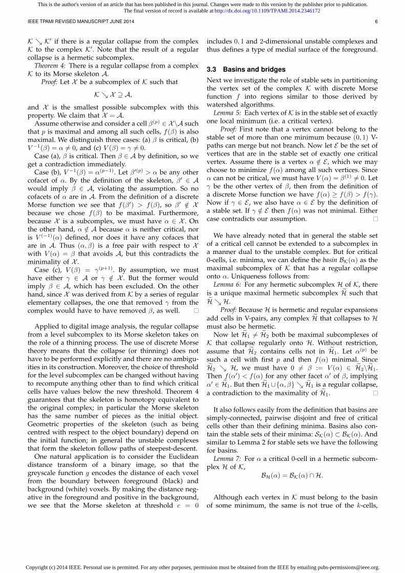
K ↘ K′ if there is a regular collapse from the complexK to the complex K′. Note that the result of a regularcollapse is a hermetic subcomplex.

Theorem 4: There is a regular collapse from a complexK to its Morse skeleton A.

Proof: Let X be a subcomplex of K such that

K ↘ X ⊇ A,

and X is the smallest possible subcomplex with thisproperty. We claim that X = A.

Assume otherwise and consider a cell β(p) ∈ X\A suchthat p is maximal and among all such cells, f(β) is alsomaximal. We distinguish three cases: (a) β is critical, (b)V −1(β) = α 6= 0, and (c) V (β) = γ 6= 0.

Case (a), β is critical. Then β ∈ A by definition, so weget a contradiction immediately.

Case (b), V −1(β) = α(p−1). Let β′(p) > α be any othercofacet of α. By the definition of the skeleton, β′ ∈ Awould imply β ∈ A, violating the assumption. So nocofacets of α are in A. From the definition of a discreteMorse function we see that f(β′) > f(β), so β′ /∈ Xbecause we chose f(β) to be maximal. Furthermore,because X is a subcomplex, we must have α ∈ X . Onthe other hand, α /∈ A because α is neither critical, noris V (−1)(α) defined, nor does it have any cofaces thatare in A. Thus (α, β) is a free pair with respect to Xwith V (α) = β that avoids A, but this contradicts theminimality of X .

Case (c), V (β) = γ(p+1). By assumption, we musthave either γ ∈ A or γ /∈ X . But the former wouldimply β ∈ A, which has been excluded. On the otherhand, since X was derived from K by a series of regularelementary collapses, the one that removed γ from thecomplex would have to have removed β, as well.

Applied to digital image analysis, the regular collapsefrom a level subcomplex to its Morse skeleton takes onthe role of a thinning process. The use of discrete Morsetheory means that the collapse (or thinning) does nothave to be performed explicitly and there are no ambigu-ities in its construction. Moreover, the choice of thresholdfor the level subcomplex can be changed without havingto recompute anything other than to find which criticalcells have values below the new threshold. Theorem 4guarantees that the skeleton is homotopy equivalent tothe original complex; in particular the Morse skeletonhas the same number of pieces as the initial object.Geometric properties of the skeleton (such as beingcentred with respect to the object boundary) depend onthe initial function; in general the unstable complexesthat form the skeleton follow paths of steepest-descent.

One natural application is to consider the Euclideandistance transform of a binary image, so that thegreyscale function g encodes the distance of each voxelfrom the boundary between foreground (black) andbackground (white) voxels. By making the distance neg-ative in the foreground and positive in the background,we see that the Morse skeleton at threshold c = 0

includes 0, 1 and 2-dimensional unstable complexes andthus defines a type of medial surface of the foreground.

3.3 Basins and bridges

Next we investigate the role of stable sets in partitioningthe vertex set of the complex K with discrete Morsefunction f into regions similar to those derived bywatershed algorithms.

Lemma 5: Each vertex of K is in the stable set of exactlyone local minimum (i.e. a critical vertex).

Proof: First note that a vertex cannot belong to thestable set of more than one minimum because (0, 1) V-paths can merge but not branch. Now let E be the set ofvertices that are in the stable set of exactly one criticalvertex. Assume there is a vertex α /∈ E , which we maychoose to minimize f(α) among all such vertices. Sinceα can not be critical, we must have V (α) = β(1) 6= 0. Letγ be the other vertex of β, then from the definition ofa discrete Morse function we have f(α) ≥ f(β) > f(γ).Now if γ ∈ E , we also have α ∈ E by the definition ofa stable set. If γ /∈ E then f(α) was not minimal. Eithercase contradicts our assumption.

We have already noted that in general the stable setof a critical cell cannot be extended to a subcomplex ina manner dual to the unstable complex. But for critical0-cells, i.e. minima, we can define the basin BK(α) as themaximal subcomplex of K that has a regular collapseonto α. Uniqueness follows from:

Lemma 6: For any hermetic subcomplex H of K, thereis a unique maximal hermetic subcomplex H such thatH ↘ H.

Proof: Because H is hermetic and regular expansionsadd cells in V-pairs, any complex H that collapses to Hmust also be hermetic.

Now let H1 6= H2 both be maximal subcomplexes ofK that collapse regularly onto H. Without restriction,assume that H2 contains cells not in H1. Let α(p) besuch a cell with first p and then f(α) minimal. SinceH2 ↘ H, we must have 0 6= β := V (α) ∈ H2\H1.Then f(α′) < f(α) for any other facet α′ of β, implyingα′ ∈ H1. But then H1∪{α, β} ↘ H1 is a regular collapse,a contradiction to the maximality of H1.

It also follows easily from the definition that basins aresimply-connected, pairwise disjoint and free of criticalcells other than their defining minima. Basins also con-tain the stable sets of their minima: SK(α) ⊂ BK(α). Andsimilar to Lemma 2 for stable sets we have the followingfor basins.

Lemma 7: For α a critical 0-cell in a hermetic subcom-plex H of K,

BH(α) = BK(α) ∩H.

Although each vertex in K must belong to the basinof some minimum, the same is not true of the k-cells,




k ≥ 1. We call a 1-cell that is not contained in any basin abridge. If β(1) is a bridge, then we must have V −1(β) = 0,so either β is critical (a 1-saddle), or V (β) 6= 0. Thenthe following result implies that every 1-cell from K iscontained either in the basin of a minimum or in thestable set of one or more 1-saddles.

Lemma 8: Every bridge is in the stable set of at leastone critical bridge.

Proof: First we show that if a bridge β is suchthat V (β) = γ 6= 0 then γ has another facet β′ < γ,β′ 6= β such that β′ is also a bridge. We will obtain acontradiction by assuming that all facets σ < γ, σ 6= βbelong to some basin. Note that if a 1-cell belongs to abasin B(α) then both its vertices must belong to the samebasin, since basins are sub-complexes. This implies thatthe facets σ all belong to the same basin. But then (β, γ)form a free pair with respect to B(α), implying that B(α)was not maximal.

Now let V be the set of all bridges that belong to stablesets of 1-saddle bridges, and pick a bridge β /∈ V withf(β) minimal. In particular, β cannot itself be a saddleand so V (β) = γ 6= 0. At least one other facet, β′ < γmust be a bridge by the above argument. Clearly, f(β′) <f(β), so β′ ∈ V and then also β ∈ V , contradicting ourassumption.

Now observe that when β is a bridge between thebasins of two minima B(α) and B(γ), the V-paths thatstart at each vertex of β form a path between α and γthat we call the canonical path defined by β. Note thatα = γ is possible and then the canonical path will behomotopic to a circle (we only have homotopy here, nothomeomorphism because (0,1) V-paths can merge). If βis a critical 1-cell, this path is the unstable complex of βand forms part of the Morse skeleton of K, so we haveestablished that when two minima are in the unstablecomplex of a 1-saddle, their basins are adjacent at that1-saddle. Notice that the converse is not true: two basinsmay be adjacent when there is no critical 1-cell bridgingtheir minima. The canonical path of a non-critical bridgecaptures this additional connectivity between minima.

A further characterisation of these canonical paths isgiven by the following.

Theorem 9: For any bridge, β, there are critical bridgesβ1, . . . , βk such that the canonical path through β canbe deformed, keeping its end-point minima fixed, to theconcatenation of canonical paths through the βi.

Proof: We first show that any path through the 1-skeleton of K is homotopic with fixed end points to onewhich does not cross any non-saddle bridges. Let ϕ bea counterexample which minimizes the largest f -valueof any non-saddle bridge crossed. Let β be the bridge inquestion. We can then find cells γ and β′ as in the proofof Lemma 8 above, and push the path across γ to obtaina new path ϕ′ which now crosses the bridge β′ withf(β′) < f(β). In fact all non-saddle bridges crossed byϕ′ must have f -values smaller than f(β). This is true forthose already crossed by ϕ by the assumed uniqueness

of f -values on cells of K and for those new to ϕ′ by thesame argument that showed f(β′) < f(β). But if ϕ wasa counterexample to the statement, so is ϕ′ and then ϕcould not have minimised the largest f -value for a non-saddle bridge crossed.

Finally, since basins are simply-connected, any pathwithin a particular basin is homotopic to any other pathwith the same end points. So the original canonical pathfrom α to α′ through β, which is deformed to some pathfrom α to α′ that passes only through critical bridges, isbroken into segments interior to a single basin. Each ofthese segments is homotopic to a path that is built fromcanonical paths of the relevant critical bridges.

4 SIMPLIFICATION

The initial watershed partition of a real image (even onewith small-amplitude noise) usually creates more basinsthan necessary to effectively summarize the structurespresent; naturally this issue also occurs when we con-struct the Morse basins of a real image. There are manystrategies presented in the literature for merging water-shed basins that are close in some sense [34], [35], [36],[37], [38]. As we saw in the previous section, adjacentbasins may or may not be connected via a 1-saddle,and identifying this is crucial to merging basins in away that preserves important topological information (asmeasured by persistent homology). Our Morse theoreticapproach uses built-in techniques for cancelling criticalpoints and the natural connection with homology meanswe can simplify the topology of the level sets in acontrolled way. As well as merging basins, Morse theoryincorporates higher-order topological changes such asfilling in extraneous loops and voids using the sametechniques.

Discrete Morse theory provides a very simple methodfor cancelling two critical cells, α(p) and β(p+1), byreversing the pairings along a V-path between them.Forman [7] shows that when there is exactly one V-path from the boundary of β to α, the modified vectorfield is a gradient vector field (if there is more thanone V-path, the reversal introduces loops). The questionnow is which critical cells should be cancelled, and thisis where we require the information from persistenthomology. Morse cancellation of critical points and theconnection with persistent homology has been studied indetail for functions on triangulations of 2-manifolds [15],[19], [39]. For three-dimensional complexes there areknown obstructions to simplifying some configurationsof persistence pairs as discussed in [19], [27], [40], [41].

We emphasise that there are two cell-complex repre-sentations of our data. The lower-level description is thecubical complex K with a discrete Morse function f , andthe higher-level description is the Morse chain complexM. The latter is the basis for the persistent homologycalculations, but it is the cubical complex where werequire a simplification operation to reduce the numberof critical cells by adjusting the discrete Morse function




and thereby merging basins, for example. The Morsechain complex is an algebraic description of the object.There is a boundary operator ∂M that records incidencesbetween critical cells that are connected via V-paths.The V-path incidences are counted with orientations andwith respect to a coefficient group; we use Z2, but otherchoices are possible, see [7] for details. This algebraicstructure means the Morse chain complex ignores cellincidences that cancel out, for example, when there aretwo V-paths between a pair of critical cells.

4.1 Persistent homology

Persistent homology captures the changes in topologyof a sequence of nested subcomplexes, i.e. a filtration.The filtration is determined by the order of insertion ofcells from the cell complex K. We write α ≺ β if α isinserted before β. To ensure each step in the filtration isa subcomplex we must have faces inserted before theircofaces: α ≺ β if α < β. The persistence of features ismeasured via a time-of-insertion function t : K → R sothat t(α) ≤ t(β) whenever α ≺ β. For example, when thefiltration is determined by level cuts of a function f wemight have

t(α) = min{c | α ∈ Kf (c)}.

Now examine what happens when a single p-cell αis added to a subcomplex Ki. The boundary of α mustalready be in Ki, so α either creates a new p-cycle or fillsin a (p− 1)-cycle. The idea behind persistent homologyis that these events are paired and define the lifetimeof a topological feature. Specifically, suppose that z isa p-cycle created by adding the cell α at time t(α) andthat z′ is a p-cycle that is homologous to z with z′ = ∂β,where β is a (p+ 1)-cell added at time t(β) ≥ t(α). Thepersistence of z, and of its homology class [z], is equalto t(β) − t(α). The cell α is called the creator and β thedestroyer of [z]. Some cycles never become boundariesand these are given infinite persistence.

4.2 Close pair cancellation

Ideally, we would like to adjust the discrete Morsefunction on the cubical complex so as to remove all low-persistence features up to a given threshold, τ . A naiveapproach to simplification might be to first determine allthese persistence pairs and then cancel out the ones withpersistence below the threshold τ . There are at least twopotential problems with this idea. Firstly, determining allcreator-destroyer pairs is relatively expensive, and sec-ondly, destroyers are not necessarily incident to creators,so it is not obvious how such a cancellation would beperformed in practice.

An alternative approach not requiring the persis-tence pairing, might be to identify pairs of critical cells(α(p), β(p+1)) in the Morse chain complex, M, whereα ∈ ∂M(β) and t(β)− t(α) ≤ τ (t is the time-of-insertionfunction for the filtration on M). In this homological

α1"

α5"α4"

α3"

α2"

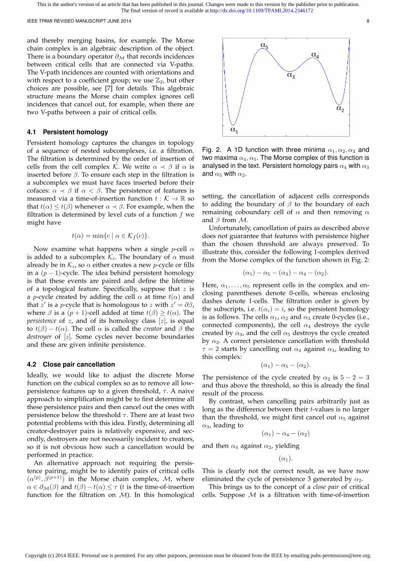
Fig. 2. A 1D function with three minima α1, α2, α3 andtwo maxima α4, α5. The Morse complex of this function isanalysed in the text. Persistent homology pairs α4 with α3

and α5 with α2.

setting, the cancellation of adjacent cells correspondsto adding the boundary of β to the boundary of eachremaining coboundary cell of α and then removing αand β from M.

Unfortunately, cancellation of pairs as described abovedoes not guarantee that features with persistence higherthan the chosen threshold are always preserved. Toillustrate this, consider the following 1-complex derivedfrom the Morse complex of the function shown in Fig. 2:

(α1)− α5 − (α3)− α4 − (α2).

Here, α1, . . . , α5 represent cells in the complex and en-closing parentheses denote 0-cells, whereas enclosingdashes denote 1-cells. The filtration order is given bythe subscripts, i.e. t(αi) = i, so the persistent homologyis as follows. The cells α1, α2 and α3 create 0-cycles (i.e.,connected components), the cell α4 destroys the cyclecreated by α3, and the cell α5 destroys the cycle createdby α2. A correct persistence cancellation with thresholdτ = 2 starts by cancelling out α4 against α3, leading tothis complex:

(α1)− α5 − (α2).

The persistence of the cycle created by α2 is 5 − 2 = 3and thus above the threshold, so this is already the finalresult of the process.

By contrast, when cancelling pairs arbitrarily just aslong as the difference between their t-values is no largerthan the threshold, we might first cancel out α5 againstα3, leading to

(α1)− α4 − (α2)

and then α4 against α2, yielding

(α1).

This is clearly not the correct result, as we have noweliminated the cycle of persistence 3 generated by α2.

This brings us to the concept of a close pair of criticalcells. Suppose M is a filtration with time-of-insertion




function t, then (α, β) form a close pair when α(p) is thelast boundary cell of β(p+1) to be added in the filtration,and β is the first coboundary cell of α to be inserted.In the example above, (α3, α4) form a close pair and(α3, α5) do not. The following two results hold:

Theorem 10: If M contains a cycle with persistence τ ,then it contains a close pair α ∈ ∂M(β) with t(β)−t(α) ≤τ .

Proof: Let us begin by assuming that the cycle inquestion is created by a cell γ and destroyed by a cell ε.If ε is not a coboundary cell of γ, there must be anothercoboundary cell, say ε′, such that γ ≺ ε′ ≺ ε and thust(ε′) − t(γ) ≤ t(ε) − t(γ) = τ . Indeed, every coboundarycell of γ must be inserted after γ, and if no coboundarycells of γ are part of the complex by the time ε is inserted,there is no way for ε to destroy the cycle created by γ.This proves that M must contain a pair with t-valuedifference no larger than τ .

Now consider a cell β and α ∈ ∂M(β) such that t(β)−t(α) ≤ τ and the number of cells inserted between αand β is minimal. Such a pair exists by the above, andbecause M is finite. Assume there is a coboundary cellβ′ of α such that β′ ≺ β. But then t(β′) ≥ t(β) andthus t(β′) − t(α) ≤ t(β) − t(α) ≤ τ , and moreover, thenumber of cells inserted between α and β′ would besmaller than the number of cells inserted between α andβ, contradicting our assumption. In the same manner,one shows that there can be no boundary cell α′ of βwith α ≺ α′, and consequently α and β must alreadyform a close pair.

Lemma 11: If α ∈ ∂M(β) form a close pair in M, thenα must create a homological cycle which is destroyed byβ.

Proof: Indeed, since α is the last boundary cell ofβ inserted, and no coboundary cell of α can be presentat the time α is added, α must create a cycle that ishomologous to the boundary of β in the cubical complex.Until β is added, there can be no chain containing α inits boundary, so that cycle must still exist, and thus isindeed destroyed by β.

Now if M contains any cycle with persistence nolarger than a threshold τ , Theorem 10 tells us thatthere exists a close pair with t-value difference also nolarger than τ , and Lemma 11 establishes that such apair must indeed form a creator-destroyer pair for ahomological cycle. Thus by performing a cancellationon the close pair, we obtain a smaller complex with thesame τ -persistent homology. If the original cycle was noteliminated in this round, the induction principle showsthat it eventually will be. In conclusion, by repeatedlycancelling out close pairs up to a given persistencethreshold, we obtain a smallest simplified complex withthe same τ -persistent homology as the original M.

As a special case, setting p = ∞ will successivelyeliminate all features of M with finite persistence andin effect generate a complete sequence of homological

creator-destroyer pairs. In this sense, simplification ofa complex via close pair cancellation in the purelyhomological setting can be viewed as a generalisationof classical persistence computation. We emphasise thatthis simplification happens on the algebraic Morse chaincomplex, not on the gradient vector field of the originalcubical complex.

Note that the above results show that close pairs arepersistence pairs, but clearly not all persistence pairsare close. Results similar to Theorem 10 and Lemma 11were first discussed for 2-dimensional simplicial com-plexes in [15], and for general cell complexes in [42].More recently, an analogous approach has been used inpersistent homology algorithms developed in [43].

In terms of the gradient vector field on the initial(cubical) complex K, a cancellable close pair (α(p), β(p+1))is a critical cell pair such that there is a single V-pathfrom the boundary of β to α, with the condition that anyother critical cell γ(p) that is reachable via a V-path fromthe boundary of β has f(γ) ≤ f(α) and similarly for anycritical cell δ(p+1) for which there is a V-path terminatingat α has f(δ) ≥ f(β). A cancellable close pair in thecubical complex must be a close pair in the Morse chaincomplex, but the converse does not always hold, becauseof the possible algebraic cancellation of paths betweencritical cells, e.g. three V-paths adding mod-2 to a singleincidence in the chain complex.

Reversing the V-path between a cancellable close pair(α, β) with persistence t(β) − t(α) < τ results in a newvector field with the same h-persistent homology as theoriginal, for h ≥ τ . However, the recursive reversal of V-paths between cancellable close pairs with t(β)−t(α) ≤ τmay not remove all homological features with persis-tence less than τ .

5 IMPLEMENTATION

We assume that a discrete gradient vector field, V , isalready defined on a given cell complex, K. For a digitalimage, with a function f defined on its voxels, this couldbe the output from the ProcessLowerStar algorithmgiven in [6]. To build a Morse skeleton and partition forf and V requires us to compute the unstable complexesand stable sets of critical cells, and also to simplify thevector field by cancelling close pairs of critical cells.Each of these operations requires us to trace V-pathsthrough the discrete vector field, particularly betweencritical cells. We present Python implementations for theessential routines required to do this efficiently below.The full code, including some examples of its usage, isavailable from the authors. For practical use, we havealso implemented several versions of these algorithmsin C++, including one that supports distributed memoryparallelism.

The algorithms shown below are implemented usingPython generators. This means that the routine perform-ing the algorithm and the code from which it is called




execute concurrently. The yield keyword is used topass results successively to the caller, which consumesthem one by one as they are produced, typically withina for loop. We chose this form for its resemblance to theoutput statement often found in pseudo-code.

We use the following parameters to represent thegradient vector field and underlying cell complex:

V A function representing a discrete vector field:

V(x) =

x if x is critical,y if x is paired with a cofacet y,∅ otherwise.

coV The reverse vector field in the same form.I A function that lists a cell’s facets.coI A function that lists a cell’s cofacets.

5.1 Vector field traversal and the Morse chain com-plex

For any pair of critical cells γ(i+1), δ(i) the Morse chaincomplex counts the number of V-paths that start in afacet of γ and end at δ. In practice, we typically do notrequire the exact counts. Instead, it is often sufficient toknow whether there is an even or odd number of paths(in order to compute homology over Z2) and whetherthere is no path, exactly one, or several (in order todetermine whether Morse cancellation can be applied).But this still leaves common graph traversal algorithmssuch as breadth-first search (BFS) unsuitable for ourpurposes without modifications.

The method proposed in [6] was to use a modified BFSthat may traverse the same edge multiple times, whichis very easy to implement and in practice often very fast,but unfortunately suffers from an exponential worst casebehaviour. This is because (1, 2) V-paths in 3D complexescan branch and re-merge, and each such branch/re-merge event leads to (at least) a two-fold increase inthe total number of paths. A better behaved algorithmwas proposed in [20], based on the following idea: in atraditional BFS, a vertex is added to the queue as soonas it is first reached via an incoming edge. If instead onewaits until it is reached for the last time, informationsuch as the total number of paths leading to this vertexcan be accumulated before being passed on further.

Depending on the value of a parameter (coordinated),our algorithm traverseFlow performs either an unmodi-fied BFS or the modified version that delays followingthe outgoing edges of a node in the graph until all itsincoming edges have been seen. We refer to the latterversion as a coordinated breadth-first search.

With coordinated false, we have a straightforward BFS.A queue, here implemented as a list, holds cells tobe processed. The set seen contains all cells that havebeen added to the queue at some point, and effectivelyensures that each cell is only processed once. Both thequeue and the set are initialised with the start cell s.The outer loop pulls the first cell a from the queue, then

the inner loop looks at each cofacet b of a in turn, firstdetermining the facet c it is paired with, if any. If c isdefined and different from a, the cell triple is returned,and c is added to the queue unless it had been addedearlier or is a critical cell, the latter being indicated byb = c.

If coordinated is true, a standard BFS first determineshow often in total each cell appears as c. This number isstored in the map nrIn. A new map k is then used, duringa second BFS pass, to count cell appearances again. Cellsare prevented from being added to the queue as long astheir nrIn and k values still differ.def traverseFlow(s, V, I, coordinated = False):

"""Produces all cell triples of the form (a, b, c),where a is in the unstable set of the cell s, bis an element of I(a), and c = V(b) != a. A cellother than s only appears as a after appearingas c at least once. If coordinated is True, itsappearances as a strictly follow those as c."""

if coordinated:nrIn = {}k = {}for (a, b, c) in traverseFlow(s, V, I):

nrIn[c] = nrIn.get(c, 0) + 1

queue = [s]seen = {s}

while len(queue) > 0:a = queue.pop(0)for b in I(a):

c = V(b)if c != a and c is not None:

yield (a, b, c)if c not in seen and c != b:

if coordinated:k[c] = k.get(c, 0) + 1if k[c] != nrIn[c]:

continuequeue.append(c)seen.add(c)

The algorithm traverseFlow is used in a variety ofcircumstances. Note that the third item c in the sequenceof cell triples traverseFlow produces ranges over theunstable set of s (with the exception of s itself), plusthe critical cells with dimension one less than s thatcan be reached by V-paths starting at facets of s (sincewe have c = V (b) = b when b is critical). Resultsfrom Section 3 show that the Morse skeleton of a levelsubcomplex is simply a union of unstable complexes forcritical cells belonging to the subcomplex, so this is allthe computation required. We can also traverse the flowin the opposite direction by passing in coV instead of Vand coI instead of I, and so compute stable sets and thusthe basins of local minima.

To obtain the homological Morse chain complex weneed to compute boundary operators as follows. Foreach cell c that can be reached by V-paths from a facetof a given critical cell s, we count the total number ofsuch paths, which is obviously the sum of path countsfor all cells from which c can be reached in a singlestep. Updating these counts in the order prescribed by




a coordinated traversal ensures that incoming countsare always correct. An exponential number of V-pathscould potentially lead to excessively large counts, sowe only store three discrete values (1, 2 for an evennumber, and 3 for all larger odd numbers) as indicatedin our implementation morseBoundary below. To accountfor the possibility of the same critical cell being reachedindependently from multiple directions, we keep track ofthese in the set boundary and only output them togetherwith their path counts after the traversal is finished.def morseBoundary(s, V, I):

"""Produces all pairs (c, k) where c is a criticalcell that can be reached from a facet of s viaV-paths, with k=1 if there is a single such pathand k>1 indicating multiple paths, with k=2 foran even and k=3 for an odd number."""

counts = { s: 1 }boundary = set()

for (a, b, c) in traverseFlow(s, V, I, True):n = counts[a] + counts.get(c, 0)counts[c] = n if n <= 3 else n % 2 + 2if b == c:

boundary.add(c)

for c in boundary:yield (c, counts[c])

5.2 SimplificationTo implement the simplification of a gradient vector fieldvia Morse cancellation of close pairs, as discussed inSection 4, we first determine all cancellable close pairsof given dimensions, which is straightforward given thelist of critical cells and the morseBoundary algorithm. Wecan introduce further conditions at this point, such as anupper limit on the persistence of a close pair.

In general, the algorithm connections given below, con-structs the union of all V-paths between a given pair (s, t)of critical cells by first marking all cells in the stable setof t via a backwards traversal, and then restricting theresults of a forward traversal accordingly.def connections(s, t, V, coV, I, coI):

"""Produces all triples of the form (a, b, c),where a is in the unstable set of the cell s, bis an element of I(a) which is also in thestable set of t, and c = V(b) != a. A cell otherthan s only appears as a after appearing as c atleast once."""

active = { t }for (a, b, c) in traverseFlow(t, coV, coI):

active.add(c)

for (a, b, c) in traverseFlow(s, V, I):if b in active:

yield (a, b, c)

For a cancellable close pair (s, t), the algorithm connec-tions yields triples (a, b, c) along the single V-path from sto t. The gradient vector field is simplified by pairing thecell b with its cofacet a, so reversing the gradient flow

along that V-path. Because of the restriction to cancellableclose pairs, all these path reversals can be performedconcurrently without influencing each other. This is dueto two properties of cancellable close pairs. First, giventwo cancellable close pairs (s1, t1) and (s2, t2) the V-pathfrom s1 to t1 cannot intersect that from s2 to t2. Second,close pairs are persistence pairs, and each critical k-cellcan either create a k-cycle or destroy a (k − 1)-cycle,but not both. In a more general setting, path reversalsbetween critical cells in a 3D discrete gradient vectorfield can cause considerable changes in the adjacenciesbetween nearby critical cells; this has been explored indetail in [27].

The new gradient vector field obtained after a sim-plification pass as described above may contain newcancellable close pairs. We therefore repeat the processuntil no further cancellable close pairs that fulfill anyadditional restrictions are found.

6 EXAMPLES

We present some examples to illustrate our methods.Table 3 shows execution times and memory consumptionfor a number of three-dimensional data sets. The firsteight, from [44], are included for comparison with [20],[45]. The remaining four were derived from binaryimages [46] by applying a signed Euclidean distancetransform, as discussed in Section 3. All computationswere performed on a single core of an Intel Core 2Duo T8100 laptop CPU running at 2.1GHz. We usedan optimised C++ implementation of the algorithmsdescribed in Section 5.

The long execution times for the simplification ofthe gradient vector field are due to the fact that ourcurrent implementation recomputes the full Morse chaincomplex after each pass. This could be improved bymodifying the algorithm to make incremental updates.We also observe that computing the chain complex tooksignificantly longer after simplification for some images,whereas for others it became faster. This is likely dueto competition between a reduction in the number ofcritical cells and an associated increase in size of thestable and unstable sets associated with the critical cells.It is clear from these results that the computational costof these methods is low enough that they can easilybe applied to multi-gigavoxel images given a parallelimplementation and the multi-core computing hardwareavailable in 2013.

Figure 4 shows our methods applied to a 2d dataset.The input data was obtained by extracting a 510x510slice from the Mt Gambier limestone image at [46]and applying a signed Euclidean distance transform onthe resulting binary 2d image. We show the resultingfeatures after simplifying the gradient vector field witha threshold of 1 pixel unit. This level of simplification issufficient to capture both large- and small-scale details ina natural way. We observe that some gradient paths tendto follow axis directions leading to partition boundaries




Name Dimensions # Critical Cells Memory (MB) Time (sec)vector simpli- chain complex vector simpli- chain complex

before after field fication before after field fication before afterSilicium 98x34x34 1109 813 1.4 1.8 1.3 1.2 0.28 0.61 0.25 0.26Fuel 64x64x64 667 135 2.5 2.9 1.5 2.0 0.67 1.36 0.13 0.30Neghip 64x64x64 5709 489 2.5 3.2 1.8 2.0 0.68 2.00 0.26 0.36Hydrogen 128x128x128 24257 17 16.9 20.7 10.8 10.1 5.58 23.83 5.33 0.80Engine 256x256x128 1035127 105573 66.0 25.4 11.5 44.3 24.60 709.07 32.65 76.02Aneurysm 256x256x256 75485 44657 131.6 145.9 71.7 79.3 44.41 2099.63 68.76 442.58Bonsai 256x256x256 344277 130033 131.6 193.9 95.4 85.5 45.56 6682.86 162.99 950.81Foot 256x256x256 1658617 1210291 131.6 425.5 194.2 163.8 46.75 2718.83 107.57 415.07Limestone 510x510x510 1708665 19133 1036.8 1343.6 649.6 521.1 345.73 1991.57 197.15 68.99Sandstone 510x510x510 2320429 61041 1036.8 1437.3 688.1 523.6 358.62 1643.09 150.67 69.69Sand Pack 510x510x510 2942231 41611 1036.8 1525.4 725.3 521.9 352.94 1586.24 126.46 57.25Sphere Pack 510x510x510 984625 3755 1036.8 1191.8 584.7 519.4 323.91 1192.34 48.00 40.16

Fig. 3. Execution times and memory consumption for some 3d images. Numbers of critical cells before and aftersimplification with persistence threshold 1 are listed. Memory consumption and execution times are given for thegradient vector field computation, simplification, and Morse chain complex computation before and after simplification.

Fig. 4. Morse analysis of a 2d Euclidean distance image(Mt. Gambier limestone). The solid phase (background) isshown in gray, and the void space (foreground) is dividedinto colored pores formed by its intersections with thebasins. Critical cells are indicated by round dots, blackfor minima, cyan for saddles, and white for maxima. TheMorse skeleton is shown in white, and other V-pathsbetween critical cells in cyan.

that do not match their intuitive best location. This is aninherent problem with discretised versions of Morse the-ory, and a technique to correct the geometric aberrationusing randomised variations in the gradient pairings ispresented in [47].

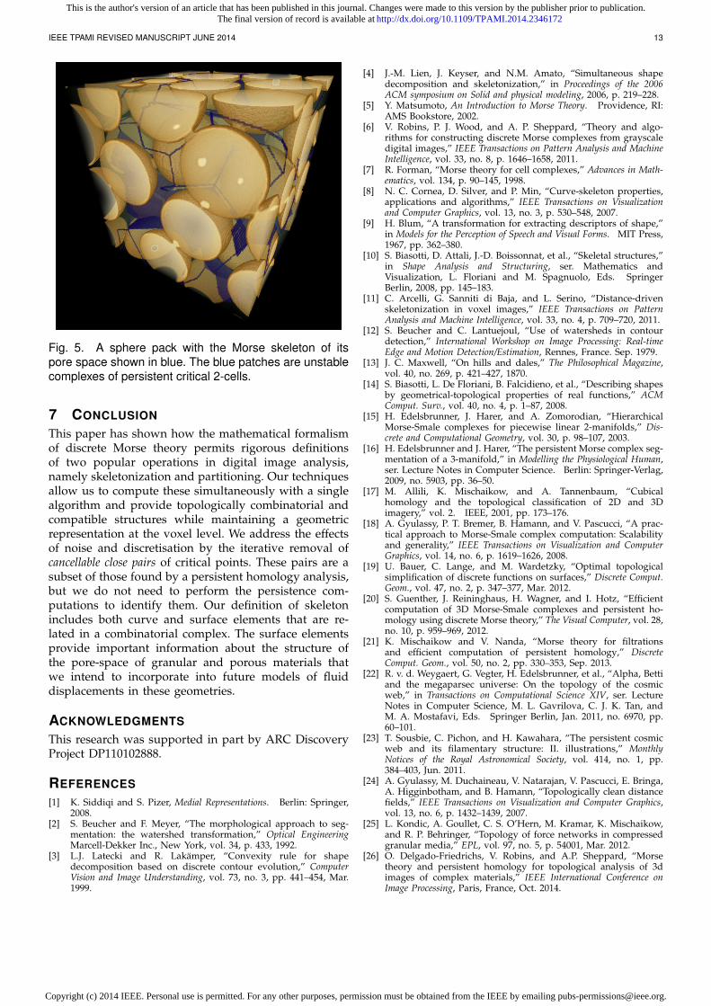
In Figure 5, we present a visualisation (using [48]) ofa silica sphere pack, also from [46], together with theMorse skeleton of its pore-space, again after simplifyingwith a threshold of 1 voxel unit. Here, we extracteda 254x254x254 section from the center of the originalimage after applying the distance transform. The Morse

skeleton contains 1-dimensional and 2-dimensional el-ements; the latter formed by unstable complexes ofcritical 2-cells. The presence of persistent critical 2-cells— each resulting in a single 2-dimensional element inthe skeleton — suggests that this pore geometry wouldbe poorly represented by a 1D line skeleton. Extractingnetworks from binary digital images of porous materi-als is commonly performed as input for pore-networkmodels that are used to simulate the flow of two orthree immiscible fluids through the pore space [49], [50].The vertices of the pore network carry weights such asthe volume of the associated pore, and the edges ofthe network have weights that determine how easy itis for fluid to move from one pore to the next. Withoutinformation about the critical 2-cells as seen in Fig. 5,such models must currently either replace each surfacepatch with a single line [49], [50], or abandon homotopyequivalence by puncturing the patch and using two ormore paths through the pore [51]. A better solutionwould be to extend the pore-network model to includethe 2-dimensional patches and an improved physicalmodel of fluid flow in these critical 2-cell pores. Whilesurface skeletons can be derived from digital images[52], such skeletons are not naturally combinatorial andtheir surface may branch in a complex manner render-ing them difficult to use for modelling applications. Acombinatorial skeleton that does contains 2-cells, wasdefined in [53] for the complement of objects built from aunion of balls. While potentially applicable to 3D digitalimages of porous materials, the method in [53] is toocomputationally intensive for routine 3D application.Our Morse skeleton is both geometrically realised as adigital object, has topologically accurate combinatorialstructure, and is dual in a rigorous sense to the Morsepartition. The persistence and geometric extent of the 2-dimensional elements associated with critical 2-cells inthe pore space will be used to provide better physicalmodelling of fluid displacements via improved pore-network models.




Fig. 5. A sphere pack with the Morse skeleton of itspore space shown in blue. The blue patches are unstablecomplexes of persistent critical 2-cells.

7 CONCLUSION

This paper has shown how the mathematical formalismof discrete Morse theory permits rigorous definitionsof two popular operations in digital image analysis,namely skeletonization and partitioning. Our techniquesallow us to compute these simultaneously with a singlealgorithm and provide topologically combinatorial andcompatible structures while maintaining a geometricrepresentation at the voxel level. We address the effectsof noise and discretisation by the iterative removal ofcancellable close pairs of critical points. These pairs are asubset of those found by a persistent homology analysis,but we do not need to perform the persistence com-putations to identify them. Our definition of skeletonincludes both curve and surface elements that are re-lated in a combinatorial complex. The surface elementsprovide important information about the structure ofthe pore-space of granular and porous materials thatwe intend to incorporate into future models of fluiddisplacements in these geometries.

ACKNOWLEDGMENTS

This research was supported in part by ARC DiscoveryProject DP110102888.

REFERENCES[1] K. Siddiqi and S. Pizer, Medial Representations. Berlin: Springer,

2008.[2] S. Beucher and F. Meyer, “The morphological approach to seg-

mentation: the watershed transformation,” Optical EngineeringMarcell-Dekker Inc., New York, vol. 34, p. 433, 1992.

[3] L.J. Latecki and R. Lakamper, “Convexity rule for shapedecomposition based on discrete contour evolution,” ComputerVision and Image Understanding, vol. 73, no. 3, pp. 441–454, Mar.1999.

[4] J.-M. Lien, J. Keyser, and N.M. Amato, “Simultaneous shapedecomposition and skeletonization,” in Proceedings of the 2006ACM symposium on Solid and physical modeling, 2006, p. 219–228.

[5] Y. Matsumoto, An Introduction to Morse Theory. Providence, RI:AMS Bookstore, 2002.

[6] V. Robins, P. J. Wood, and A. P. Sheppard, “Theory and algo-rithms for constructing discrete Morse complexes from grayscaledigital images,” IEEE Transactions on Pattern Analysis and MachineIntelligence, vol. 33, no. 8, p. 1646–1658, 2011.

[7] R. Forman, “Morse theory for cell complexes,” Advances in Math-ematics, vol. 134, p. 90–145, 1998.

[8] N. C. Cornea, D. Silver, and P. Min, “Curve-skeleton properties,applications and algorithms,” IEEE Transactions on Visualizationand Computer Graphics, vol. 13, no. 3, p. 530–548, 2007.

[9] H. Blum, “A transformation for extracting descriptors of shape,”in Models for the Perception of Speech and Visual Forms. MIT Press,1967, pp. 362–380.

[10] S. Biasotti, D. Attali, J.-D. Boissonnat, et al., “Skeletal structures,”in Shape Analysis and Structuring, ser. Mathematics andVisualization, L. Floriani and M. Spagnuolo, Eds. SpringerBerlin, 2008, pp. 145–183.

[11] C. Arcelli, G. Sanniti di Baja, and L. Serino, “Distance-drivenskeletonization in voxel images,” IEEE Transactions on PatternAnalysis and Machine Intelligence, vol. 33, no. 4, p. 709–720, 2011.

[12] S. Beucher and C. Lantuejoul, “Use of watersheds in contourdetection,” International Workshop on Image Processing: Real-timeEdge and Motion Detection/Estimation, Rennes, France. Sep. 1979.

[13] J. C. Maxwell, “On hills and dales,” The Philosophical Magazine,vol. 40, no. 269, p. 421–427, 1870.

[14] S. Biasotti, L. De Floriani, B. Falcidieno, et al., “Describing shapesby geometrical-topological properties of real functions,” ACMComput. Surv., vol. 40, no. 4, p. 1–87, 2008.

[15] H. Edelsbrunner, J. Harer, and A. Zomorodian, “HierarchicalMorse-Smale complexes for piecewise linear 2-manifolds,” Dis-crete and Computational Geometry, vol. 30, p. 98–107, 2003.

[16] H. Edelsbrunner and J. Harer, “The persistent Morse complex seg-mentation of a 3-manifold,” in Modelling the Physiological Human,ser. Lecture Notes in Computer Science. Berlin: Springer-Verlag,2009, no. 5903, pp. 36–50.

[17] M. Allili, K. Mischaikow, and A. Tannenbaum, “Cubicalhomology and the topological classification of 2D and 3Dimagery,” vol. 2. IEEE, 2001, pp. 173–176.

[18] A. Gyulassy, P. T. Bremer, B. Hamann, and V. Pascucci, “A prac-tical approach to Morse-Smale complex computation: Scalabilityand generality,” IEEE Transactions on Visualization and ComputerGraphics, vol. 14, no. 6, p. 1619–1626, 2008.

[19] U. Bauer, C. Lange, and M. Wardetzky, “Optimal topologicalsimplification of discrete functions on surfaces,” Discrete Comput.Geom., vol. 47, no. 2, p. 347–377, Mar. 2012.

[20] S. Guenther, J. Reininghaus, H. Wagner, and I. Hotz, “Efficientcomputation of 3D Morse-Smale complexes and persistent ho-mology using discrete Morse theory,” The Visual Computer, vol. 28,no. 10, p. 959–969, 2012.

[21] K. Mischaikow and V. Nanda, “Morse theory for filtrationsand efficient computation of persistent homology,” DiscreteComput. Geom., vol. 50, no. 2, pp. 330–353, Sep. 2013.

[22] R. v. d. Weygaert, G. Vegter, H. Edelsbrunner, et al., “Alpha, Bettiand the megaparsec universe: On the topology of the cosmicweb,” in Transactions on Computational Science XIV, ser. LectureNotes in Computer Science, M. L. Gavrilova, C. J. K. Tan, andM. A. Mostafavi, Eds. Springer Berlin, Jan. 2011, no. 6970, pp.60–101.

[23] T. Sousbie, C. Pichon, and H. Kawahara, “The persistent cosmicweb and its filamentary structure: II. illustrations,” MonthlyNotices of the Royal Astronomical Society, vol. 414, no. 1, pp.384–403, Jun. 2011.

[24] A. Gyulassy, M. Duchaineau, V. Natarajan, V. Pascucci, E. Bringa,A. Higginbotham, and B. Hamann, “Topologically clean distancefields,” IEEE Transactions on Visualization and Computer Graphics,vol. 13, no. 6, p. 1432–1439, 2007.

[25] L. Kondic, A. Goullet, C. S. O’Hern, M. Kramar, K. Mischaikow,and R. P. Behringer, “Topology of force networks in compressedgranular media,” EPL, vol. 97, no. 5, p. 54001, Mar. 2012.

[26] O. Delgado-Friedrichs, V. Robins, and A.P. Sheppard, “Morsetheory and persistent homology for topological analysis of 3dimages of complex materials,” IEEE International Conference onImage Processing, Paris, France, Oct. 2014.




[27] D. Guenther, J. Reininghaus, H.-P. Seidel, and T. Weinkauf,“Notes on the simplification of the Morse-Smale complex,” inTopological Methods in Data Analysis and Visualization III, ser.Mathematics and Visualization, P.-T. Bremer, I. Hotz, V. Pascucci,and R. Peikert, Eds. Springer, Berlin. Jan. 2014, pp. 135–150.

[28] V. A. Kovalevsky, “Finite topology as applied to image analysis,”Comput. Vision Graph. Image Process., vol. 46, no. 2, p. 141–161,1989.

[29] V. Robins, “Algebraic Topology,” in Mathematical Tools for Physi-cists. 2nd Edition, Berlin: Wiley, 2014, pp. 211–238.

[30] H. Edelsbrunner and J. Harer, Computational Topology: An introduc-tion. Providence, Rhode Island: American Mathematical Society,2010.

[31] R. Forman, “A user’s guide to discrete Morse theory,” SeminaireLotharingien de Combinatoire, vol. 48, 2002.

[32] J. H. C. Whitehead, “Simplicial spaces, nuclei, and m-groups,”Proc. London Math. Soc., vol. 45, no. 2, pp. 243–327, 1939.

[33] T. Lewiner, “Geometric discrete Morse complexes,” Ph.D. dis-sertation, Department of Mathematics, PUC-Rio, 2005. [Online].Available: http://www.matmidia.mat.puc-rio.br/tomlew/pdfs/phd thesis puc.pdf

[34] F. Meyer and S. Beucher, “Morphological segmentation,” Journalof Visual Communication and Image Representation, vol. 1, no.1, pp. 2146, 1990.

[35] S. Beucher, “Watershed, hierarchical segmentation and waterfallalgorithm,” in Mathematical Morphology and Its Applications toImage Processing, ser. Computational Imaging and Vision, J. Serraand P. Soille, Eds. Springer Netherlands, Jan. 1994, no. 2, pp.69–76.

[36] M. Couprie and G. Bertrand, “Topological gray-scale watershedtransformation,” Optical Science, Engineering and Instrumentation’97, pp. 136–146, Oct. 1997.

[37] K. Haris, S. Efstratiadis, and N. Maglaveras, “Watershed-basedimage segmentation with fast region merging,” in InternationalConference on Image Processing, 1998, pp. 338–342 vol.3.

[38] A. Bleau and L. Leon, “Watershed-based segmentation and regionmerging,” Computer Vision and Image Understanding, vol. 77, no. 3,pp. 317–370, Mar. 2000.

[39] T. Lewiner, “Critical sets in discrete Morse theories: Relating For-man and piecewise-linear approaches,” Computer Aided GeometricDesign, vol. 30, pp. 609–621, 2013.

[40] N. Shivashankar and V. Natarajan, “Parallel computation of 3DMorse-Smale complexes,” Computer Graphics Forum, vol. 31, pp.965–974, Jun. 2012.

[41] A. Gyulassy, V. Natarajan, V. Pascucci, and B. Hamann, “Efficientcomputation of Morse-Smale complexes for three-dimensionalscalar functions,” IEEE Transactions on Visualization and ComputerGraphics, vol. 13, no. 6, p. 1440–1447, 2007.

[42] H. King, K. Knudson, and N. Mramor, “Genering discrete Morsefunctions from point data,” Experimental Mathematics, vol. 14, pp.435–444, 2005.

[43] U. Bauer, M. Kerber, and J. Reininghaus, “Clear and compress:Computing persistent homology in chunks,” in TopologicalMethods in Data Analysis and Visualization III, ser. Mathematicsand Visualization, P.-T. Bremer, I. Hotz, V. Pascucci, andR. Peikert, Eds. Springer, Jan. 2014, pp. 103–117.

[44] M. Meissner, “Volvis: Voxel data repository,” 2001. [Online].Available: http://volvis.org

[45] H. Wagner, C. Chen, and E. Vucini, “Efficient computation ofpersistent homology for cubical data,” in Topological Methodsin Data Analysis and Visualization II, ser. Mathematics andVisualization, R. Peikert, H. Hauser, H. Carr, and R. Fuchs, Eds.Springer Berlin, Jan. 2012, pp. 91–106.

[46] A.P. Sheppard, “The network generation comparison forum,”2005. [Online]. Available: http://xct.anu.edu.au/networkcomparison.

[47] A. Gyulassy, P. Bremer, and V. Pascucci, “Computing Morse-Smale complexes with accurate geometry,” IEEE Transactions onVisualization and Computer Graphics, vol. 18, no. 12, pp. 2014–2022,Dec. 2012.

[48] D. Whitehouse, “Voluminous - the web based volume renderer,”Dec. 2013. [Online]. Available: http://voluminous.nci.org.au

[49] M. Prodanovic, W. Lindquist, and R. Seright, “3D image-basedcharacterization of fluid displacement in a Berea core,” Advancesin Water Resources, vol. 30, no. 2, pp. 214–226, Feb. 2007.

[50] S. Bakke and P. Oren, “3-d pore-scale modelling of sandstonesand flow simulations in the pore networks,” SPE Journal, vol. 2,no. 2, pp. 136–149, 1997.

[51] D. Silin and T. Patzek, “Pore space morphology analysis usingmaximal inscribed spheres,” Physica A: Statistical Mechanics andits Applications, vol. 371, no. 2, pp. 336–360, 2006.

[52] G. Borgefors, I. Nystrom, and G. S. d. Baja, “Skeletonizingvolume objects part II: from surface to curve skeleton,” inAdvances in Pattern Recognition, ser. Lecture Notes in ComputerScience, A. Amin, D. Dori, P. Pudil, and H. Freeman, Eds.Springer Berlin, 1998, pp. 220–229.

[53] R. Glantz and M. Hilpert, “Tight dual models of pore spaces,”Advances in Water Resources, vol. 31, no. 5, pp. 787–806, 2008.

Olaf Delgado-Friedrichs Olaf Delgado-Friedrichs received his M.Sc., PhD and Dr.habil.degrees in Mathematics at the University ofBielefeld in 1990, 1994 and 2002. He has heldresearch positions at the University of Bielefeld,the Arizona State University, the Universityof Tubingen, and the Australian NationalUniversity. Since 2012, he works as a contractorbased in Melbourne, Australia. His researchinterests are in discrete and computationalmathematics and its applications.

Vanessa Robins Vanessa Robins completedher B.Sc.(Hons) degree in Mathematics at theAustralian National University in 1994 and re-ceived her Ph.D. degree in Applied Mathematicsfrom the University of Colorado, Boulder in 2000.She has been a research fellow in the Depart-ment of Applied Mathematics at the AustralianNational University since 2000. Her researchinterests are in computational topology and ge-ometry, and the enumeration and classificationof periodic nets. She works on mathematical

foundations, algorithms and scientific applications in both these fields.

Adrian Sheppard Adrian Sheppard completedhis B.Sc (hons) degree in Mathematical Physicsat The University of Adelaide in 1992 and hisPhD degree in Physics at the Australian NationalUniversity in 1996. He has held research posi-tions at the Universite Libre de Bruxelles, theUniversity Of New South Wales and the Aus-tralian National University, where he has workedsince 2000. His research interests include thecharacterisation of shape, fluid flow in porousmedia, parallel algorithms for image processing

and tomographic imaging.



IEEE TPAMI REVISED MANUSCRIPT JUNE 2014 1 … · IEEE TPAMI REVISED MANUSCRIPT JUNE 2014 1...

Documents

Transcript of IEEE TPAMI REVISED MANUSCRIPT JUNE 2014 1 … · IEEE TPAMI REVISED MANUSCRIPT JUNE 2014 1...