IEEE 802.11 Ad Hoc Networks: Protocols, …...1 IEEE 802.11 Ad Hoc Networks: Protocols, Performance...
63
1 IEEE 802.11 Ad Hoc Networks: Protocols, Performance and Open Issues Giuseppe Anastasi Dept. of Information Engineering University of Pisa Via Diotisalvi 2 - 56122 Pisa - Italy Email: [email protected] Marco Conti, Enrico Gregori Istituto IIT National Research Council (CNR) Via G. Moruzzi 1 - 56124 Pisa - Italy Email: {marco.conti, enrico.gregori}@iit.cnr.it 1. Introduction The previous chapter has presented the activities of the different task groups within the IEEE 802.11 project [IEE], and has highlighted that the IEEE 802.11 is currently the most mature technology for infrastructure-based Wireless LANs (WLANs). The IEEE 802.11 standard defines two operational modes for WLANs: infrastructure-based and infrastructure-less or ad hoc. Network interface cards can be set to work in either of these modes but not in both simultaneously. The infrastructure-based is the mode commonly used to construct the so called Wi-Fi hotspots, i.e., to provide wireless access to the Internet. The drawbacks of an infrastructure-based WLAN are the costs associated with purchasing and installing the infrastructure. These costs may not be acceptable for dynamic environments where people and/or vehicles need to be temporarily interconnected in areas without a pre-existing communication infrastructure (e.g., inter-vehicular and disaster networks), or where the infrastructure cost is not justified (e.g., in-building networks, specific residential communities networks, etc.). In these cases, a more efficient solution can be provided by the infrastructure- less or ad hoc mode. When operating in this mode stations are said to form an Independent Basic Service Set (IBSS) or, more simply, an ad hoc network. Any station that is within the transmission range of any other, after a synchronization phase, can start communicating. No Access Point (AP) is
Transcript of IEEE 802.11 Ad Hoc Networks: Protocols, …...1 IEEE 802.11 Ad Hoc Networks: Protocols, Performance...

1
IEEE 802.11 Ad Hoc Networks: Protocols, Performance
and Open Issues
Giuseppe Anastasi Dept. of Information Engineering
University of Pisa Via Diotisalvi 2 - 56122 Pisa - Italy
Email: [email protected]
Marco Conti, Enrico Gregori Istituto IIT
National Research Council (CNR) Via G. Moruzzi 1 - 56124 Pisa - Italy
Email: {marco.conti, enrico.gregori}@iit.cnr.it
1. Introduction
The previous chapter has presented the activities of the different task groups within the IEEE
802.11 project [IEE], and has highlighted that the IEEE 802.11 is currently the most mature
technology for infrastructure-based Wireless LANs (WLANs). The IEEE 802.11 standard
defines two operational modes for WLANs: infrastructure-based and infrastructure-less or ad
hoc. Network interface cards can be set to work in either of these modes but not in both
simultaneously. The infrastructure-based is the mode commonly used to construct the so
called Wi-Fi hotspots, i.e., to provide wireless access to the Internet. The drawbacks of an
infrastructure-based WLAN are the costs associated with purchasing and installing the
infrastructure. These costs may not be acceptable for dynamic environments where people
and/or vehicles need to be temporarily interconnected in areas without a pre-existing
communication infrastructure (e.g., inter-vehicular and disaster networks), or where the
infrastructure cost is not justified (e.g., in-building networks, specific residential communities
networks, etc.). In these cases, a more efficient solution can be provided by the infrastructure-
less or ad hoc mode.
When operating in this mode stations are said to form an Independent Basic Service Set
(IBSS) or, more simply, an ad hoc network. Any station that is within the transmission range
of any other, after a synchronization phase, can start communicating. No Access Point (AP) is
2
required, but if one of the stations operating in the ad hoc mode also has a connection to the
wired network, stations forming the ad hoc network have a wireless access to the Internet.
The IEEE 802.11 technology is a good platform to implement single-hop ad hoc networks
because of its extreme simplicity. Single-hop means that stations must be within the same
transmission radium (say 100-200 meters) to be able to communicate. This limitation can be
overcome by multi-hop ad hoc networking. This requires the addition of routing mechanisms
at stations so that they can forward packets towards the intended destination, thus extending
the range of the ad hoc network beyond the transmission radium of the source station. Routing
solutions designed for wired networks (e.g., the Internet) are not suitable for the ad hoc
environment, primarily due to the dynamic topology of ad hoc networks.
In a pure ad hoc networking environment, the users’ mobile devices are the network and they
must co-operatively provide the functionality that is usually provided by the network
infrastructure (e.g. routers, switches, and servers). This approach requires that the users’
density is high enough to guarantee the packets forwarding among the sender and the
receiver. When the users’ density is low networking may become unfeasible.
Even though large-scale multi-hop ad hoc networks will not be available in the near future, on
smaller scales, mobile ad hoc networks are starting to appear thus extending the range of the
IEEE 802.11 technology over multiple radio hops. Most of the existing IEEE 802.11-based ad
hoc networks have been developed in the academic environment, but recently even
commercial solutions have been proposed (see, e.g., MeshNetworks1 and SPANworks2).
Other than being a solution for pure ad hoc networking, the IEEE 802.11 ad hoc technology
may also constitute an important and promising building block for solving the first mile
problem in hot spots. This aspect is related to the understanding of some basic Radio
1 http://www.meshnetworks.com 2 http://www.spanworks.com

3
Frequency (RF) transmission principles. Specifically, the transmission range is limited since
the RF energy disperses as the distance from the transmitter increases. In addition, even
though WLANs operate in the unregulated spectrum (i.e., the users are not required to be
licensed), the transmitter power is limited by the regulatory bodies (e.g., FCC in USA and
ETSI in Europe). IEEE 802.11a and IEEE 802.11b can operate at several bit rates but since
the transmitter power is limited the transmission range decreases when the data rate is
increased.
It is expected that the bandwidth request in hot spots will increase very fast thus requiring
higher speed access technologies. As explained in the previous chapter in this book, channel
speeds for the IEEE 802.11 family continue to increase: 802.11a operates at 54 Mbps, and
enhanced versions operating at speeds up to 108 Mbps are also under investigation. Such
high-speed WLAN standards are expected to further increase the popularity of wireless access
to the backbone infrastructure. On the other hand, increasing the transmission rate (while
maintaining the same transmission power) produces a reduction in the coverage area of an
AP. Specifically, at 100 Mbps rate the coverage area will correspond to a radius of few meters
around the AP. It seems not a feasible solution to spread in a hot spot a large number of APs
uniformly and closely spaced. A more feasible solution may be based on the use of a relative
low number of multi-rate APs, and the deployment of multi-hop wireless networks that
provides access to the wired backbone via multiple wireless hops. When the population in a
hot spot is low, the AP can use low transmission rates thus covering a large area. In this case,
the users devices can contact the AP directly (i.e., single-hop). When the hot-spot population
increases, the data rate is increased as well, and hence some devices cannot anymore directly
contact the AP but they need to be supported by other devices for forwarding their traffic
towards the AP. By further increasing the data rate, more users can be accommodated in the
hot spot but, at the same time, more hops may be necessary for user traffic to reach the AP.

4
Currently, the widespread use of IEEE 802.11 cards makes this technology the most
interesting off-the-shelf enabler for ad hoc networks. However, the standardization efforts
concentrated on solutions for infrastructure-based WLANs, while little or no attention was
given to the ad hoc mode. Therefore, the aim of this chapter is triple: (i) an in-depth
investigation of the ad hoc features of the IEEE 802.11 standard, (ii) an analysis of the
performance of 802.11-based ad hoc networks; and (iii) an investigation of the major
problems arising when using the 802.11 technology for ad hoc networks, and possible
directions for enhancing this technology for a better support of the ad hoc networking
paradigm.
The rest of the chapter is organized as follows. The next section briefly describes the
architecture and protocols of IEEE 802.11 WLANs. The aim is to introduce the terminology
and present the concepts that are relevant throughout the chapter. The interested reader can
found the details on the IEEE 802.11 protocols in the standard documents [IEE99].
The characteristics of the wireless medium and the dynamic nature of ad hoc networks make
(IEEE 802.11) multi-hop networks fundamentally different from wired networks.
Furthermore, the behavior of an ad hoc network that relies upon a carrier-sensing random
access protocol, such as the IEEE 802.11, is further complicated by the presence of hidden
stations, exposed stations, “capturing” phenomena [XuS01, XuS02], and so on. The
interaction between all these phenomena makes the behavior of IEEE 802.11 ad hoc networks
very complex to predict. Recently, this has generated an extensive literature related to the
performance analysis of the 802.11 MAC protocol in the ad hoc environment that we
surveyed in Section 3. Most of these studies have been done through simulation. To the best
of our knowledge, only very few experimental analysis have been conducted. For this reason,
in Section 4 we extend the 802.11 performance analysis with an extensive set of

5
measurements that we have performed on a real testbed. These measurements were performed
both in indoor and outdoor environments, and in the presence of different traffic types. For
the sake of comparison with the previous studies, our analysis is mostly related to the basic
IEEE 802.11 MAC protocol (i.e., we consider a data rates of 2 Mbps). However, some results
related to IEEE 802.11b are also included in Section 5. In the same section, we present some
problems (gray zones) that may occur by using IEEE 802.11b in multi hop ad hoc networks.
Finally, in Section 6 we discuss some possible extensions to the IEEE 802.11 MAC protocol
to improve its performance in multi-hop ad hoc networks.
2. IEEE 802.11 Architecture and Protocols
In this section we will focus on the IEEE 802.11 architecture and protocols as defined in the
original standard [IEE99], with a particular attention to the MAC layer. Later, in Section 5,
we will emphasize the differences between the 802.11b standard with respect to the original
802.11 standard.
Physical Layer
contention freeservices contention
services
Distributed CoordinationFunction
Point CoordinationFunction
Figure 1. IEEE 802.11 Architecture.
The IEEE 802.11 standard specifies both the MAC layer and the Physical Layer (see Figure
1). The MAC layer offers two different types of service: a contention free service provided by
the Distributed Coordination Function (DCF), and a contention-free service implemented by
the Point Coordination Function (PCF). These service types are made available on top of a
variety of physical layers. Specifically, three different technologies have been specified in the
6
standard: Infrared (IF), Frequency Hopping Spread Spectrum (FHSS) and Direct Sequence
Spread Spectrum (DSSS).
The DCF provides the basic access method of the 802.11 MAC protocol and is based on a
Carrier Sense Multiple Access with Collision Avoidance (CSMA/CA) scheme. The PCF is
implemented on top of the DCF and is based on a polling scheme. It uses a Point Coordinator
that cyclically polls stations, giving them the opportunity to transmit. Since the PCF can not
be adopted in ad hoc mode, it will not be considered hereafter.
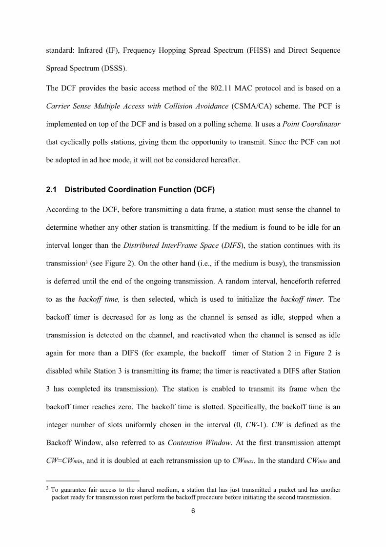
2.1 Distributed Coordination Function (DCF)
According to the DCF, before transmitting a data frame, a station must sense the channel to
determine whether any other station is transmitting. If the medium is found to be idle for an
interval longer than the Distributed InterFrame Space (DIFS), the station continues with its
transmission3 (see Figure 2). On the other hand (i.e., if the medium is busy), the transmission
is deferred until the end of the ongoing transmission. A random interval, henceforth referred
to as the backoff time, is then selected, which is used to initialize the backoff timer. The
backoff timer is decreased for as long as the channel is sensed as idle, stopped when a
transmission is detected on the channel, and reactivated when the channel is sensed as idle
again for more than a DIFS (for example, the backoff timer of Station 2 in Figure 2 is
disabled while Station 3 is transmitting its frame; the timer is reactivated a DIFS after Station
3 has completed its transmission). The station is enabled to transmit its frame when the
backoff timer reaches zero. The backoff time is slotted. Specifically, the backoff time is an
integer number of slots uniformly chosen in the interval (0, CW-1). CW is defined as the
Backoff Window, also referred to as Contention Window. At the first transmission attempt
CW=CWmin, and it is doubled at each retransmission up to CWmax. In the standard CWmin and
3 To guarantee fair access to the shared medium, a station that has just transmitted a packet and has another
packet ready for transmission must perform the backoff procedure before initiating the second transmission.

7
CWmax values depend on the physical layer adopted. For example, for the FHSS Phisical
Layer Cwmin and Cwmax values are 16 and 1024, respectively [IEE99].
Station 1
Station 2
Station 3
FRAME
DIFS
FRAME
FRAME
DIFS DIFS
Packet Arrival
Frame Transmission
Elapsed Backoff Time
Residual Backoff Time
Figure 2. Basic Access Mechanism.
Obviously, it may happen that two or more stations start transmitting simultaneously and a
collision occurs. In the CSMA/CA scheme, stations are not able to detect a collision by
hearing their own transmissions (as in the CSMA/CD protocol used in wired LANs).
Therefore, an immediate positive acknowledgement scheme is employed to ascertain the
successful reception of a frame. Specifically, upon reception of a data frame, the destination
station initiates the transmission of an acknowledgement frame (ACK) after a time interval
called Short InterFrame Space (SIFS). The SIFS is shorter than the DIFS (see Figure 3) in
order to give priority to the receiving station over other possible stations waiting for
transmission. If the ACK is not received by the source station, the data frame is presumed to
have been lost, and a retransmission is scheduled. The ACK is not transmitted if the received
packet is corrupted. A Cyclic Redundancy Check (CRC) algorithm is used for error detection.
Source Station
Destination Station
FRAME
DIFS SIFS
ACK
Packet Arrival

8
Figure 3. Interaction between the source and destination stations. The SIFS is shorter than the DIFS.
After an erroneous frame is detected (due to collisions or transmission errors), a station must
remain idle for at least an Extended InterFrame Space (EIFS) interval before it reactivates the
backoff algorithm. Specifically, the EIFS shall be used by the DCF whenever the physical
layer has indicated to the MAC that a frame transmission was begun that did not result in the
correct reception of a complete MAC frame with a correct FCS value. Reception of an error-
free frame during the EIFS re-synchronizes the station to the actual busy/idle state of the
medium, so the EIFS is terminated and normal medium access (using DIFS and, if necessary,
backoff) continues following reception of that frame.
2.2 Common Problems in Wireless Ad Hoc Networks
In this section we discuss some problems that can arise in wireless networks, mainly in the ad
hoc mode. The characteristics of the wireless medium make wireless networks fundamentally
different from wired networks. Specifically, as indicated in [IEE99]:
- the wireless medium has neither absolute nor readily observable boundaries outside
of which stations are known to be unable to receive network frames;
- the channel is unprotected from outside signals;
- the wireless medium is significantly less reliable than wired media;
- the channel has time-varying and asymmetric propagation properties.
In wireless (ad hoc) network that relies upon a carrier-sensing random access protocol, like
the IEEE 802.11 DCF protocol, the wireless medium characteristics generate complex
phenomena such as the hidden-station and exposed-station problems.
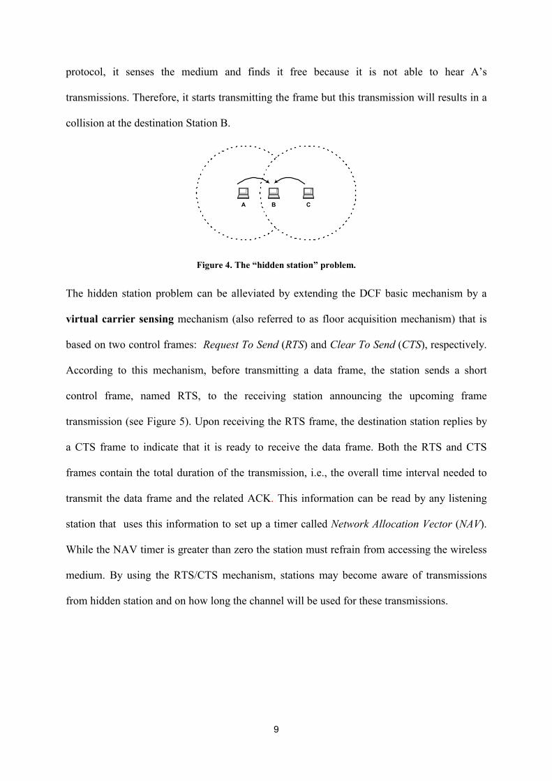
Figure 4 shows a typical “hidden station” scenario. Let us assume that station B is in the
transmitting range of both A and C, but A and C cannot hear each other. Let us also assume
that A is transmitting to B. If C has a frame to be transmitted to B, according to the DFC
9
protocol, it senses the medium and finds it free because it is not able to hear A’s
transmissions. Therefore, it starts transmitting the frame but this transmission will results in a
collision at the destination Station B.
A CB
Figure 4. The “hidden station” problem.
The hidden station problem can be alleviated by extending the DCF basic mechanism by a
virtual carrier sensing mechanism (also referred to as floor acquisition mechanism) that is
based on two control frames: Request To Send (RTS) and Clear To Send (CTS), respectively.
According to this mechanism, before transmitting a data frame, the station sends a short
control frame, named RTS, to the receiving station announcing the upcoming frame
transmission (see Figure 5). Upon receiving the RTS frame, the destination station replies by
a CTS frame to indicate that it is ready to receive the data frame. Both the RTS and CTS
frames contain the total duration of the transmission, i.e., the overall time interval needed to
transmit the data frame and the related ACK. This information can be read by any listening
station that uses this information to set up a timer called Network Allocation Vector (NAV).
While the NAV timer is greater than zero the station must refrain from accessing the wireless
medium. By using the RTS/CTS mechanism, stations may become aware of transmissions
from hidden station and on how long the channel will be used for these transmissions.

10
Source Station
Destin. Station
Another Station
FRAME
DIFS
SIFS
DIFS
SIFS
SIFS
ACK
RTS
CTS
Backoff TimeNAV RTS
NAV CTS
Figure 5. Virtual Career Sensing mechanism.
Figure 6 depicts a typical scenario where the “exposed station” problem may occur. Let us
assume that both Station A and Station C can hear transmissions from B, but Station A can
not hear transmissions from C. Let us also assume that Station B is transmitting to Station A
and Station C receives a frame to be transmitted to D. According to the DCF protocol, C
senses the medium and finds it busy because of B’s transmission. Therefore, it refrains from
transmitting to C although this transmission would not cause a collision at A. The “exposed
station” problem may thus result in a throughput reduction.
DBA C
Figure 6. The “exposed station” problem
2.3 Ad Hoc Networking Support
In this section we will describe how two or more 802.11 stations set up an ad hoc network. In
the IEEE 802.11 standard, an ad hoc network is named Independent Basic Service Set (IBSS).
An IBSS enables two or more 802.11 stations to communicate each other without the

11
intervention of either a centralized AP, or an infrastructure network. Hence, the IBSS can be
considered as the support provided by the 802.11 standard for mobile ad hoc networking.4
Due to the flexibility of the CSMA/CA protocol, to receive and transmit data correctly it is
sufficient that all stations within the IBSS are synchronized to a common clock. The standard
specifies a Timing Synchronization Function (TSF) to achieve clock synchronization between
stations. In an infra-structured network the clock synchronization is provided by the AP, and
all stations synchronizes their own clock to the AP’s clock. In an IBSS, due to the lack a
centralized station, clock synchronization is achieved through a distributed algorithm. In both
cases synchronization is obtained by transmitting special frames, called beacons, containing
timing information.
The TSF requires two fundamental functionalities, namely synchronization maintenance
and synchronization acquirement, that will be sketched below. We only focus on IBSS.
2.3.1 Synchronization maintenance.
Each station has a TSF timer (clock) with modulus 264 counting in increments of
microseconds. Stations expect to receive beacons at a nominal rate defined by the a
BeaconPeriod parameter. This parameter is decided by the station initiating the IBSS, and is
then used by any other station joining the IBSS. Stations use their TSF timers to determine the
beginning of beacon intervals or periods. At the beginning of a beacon interval each station
performs the following procedure:
i. it suspends the decrementing of the backoff timer for any pending (non-beacon)
transmission;
4 To uniquely identify a IBSS it is necessary to associate to it an identification number (IBSSID) that is locally
administered and that will be used by any other Station to join the IBSS, i.e., the ad hoc network. When a station starts a new IBSS, it generates a 46-bit random number in a manner that minimizes the probability that the same number is generated by another station.
12
ii. it generates a random delay interval uniformly distributed in the range between zero
and twice the minimum value of the Contention Window.
iii. it waits for the random delay;
iv. if a beacon arrives before the random delay timer has expired, it stops the random
delay timer, cancel the pending beacon transmission, and resumes the backoff timer;
v. if the random delay timer has expired and no beacon has been received, it sends a
beacon frame.
The sending station sets the beacon timestamp to the value of its TSF timer at the time the
beacon is transmitted. Upon reception of a beacon, the receiving station looks at the
timestamp. If the beacon timestamp is later than the station’s TSF timer, the TSF timer is set
to the value of the received timestamp. In other words, all stations within the IBSS
synchronize their TSF timer to the quickest TSF timer.
2.3.2 Synchronization acquirement.
This functionality is necessary when a station wants to join an already existing IBSS. The
discovery of existing IBSSs is the result of a scanning procedure of the wireless medium
during which the station receiver is tuned to different radio frequencies, looking for particular
control frames. Only if the scanning procedure does not result in finding any IBSS, the station
may start with the creation of a new IBSS. The scanning procedure can be either passive or
active.
In a passive scanning the station listens to the channels for hearing a beacon frame. It is worth
reminding that a beacon frame contains not only timing information for synchronization, but
also the complete set of IBSS parameters. This set includes the IBSS identifier IBSSID, the
aBeaconPeriod parameter, the data rates that can be supported, the parameters relevant to
IBSS management functions (e.g., power saving management).
13
Active scanning involves the generation of Probe frames, and the subsequent processing of
received Probe Response frames. The station that decides to start an active scanning
procedure has a ChannelList of radio frequencies that will be scanned during the procedure.
For each channel to be scanned a probe with broadcast destination and is sent by using the
DCF access method. At the same time a ProbeTimer is started. If no response to the probe is
received before the ProbeTimer reaches the MinChannelTime the next channel of the list is
considered. Otherwise, the station continues to scan the same channel until the timer reaches
the MaxChannelTime. Then, the station processes all received Probe responses.
Probe responses are sent using normal frame transmission rules as directed frames to the
address of the station that generated the Probe request. In an IBSS, only the station that
generated the last beacon transmission will respond to a probe request, in order to avoid the
waste of bandwidth with repetitive control frames. In each IBSS, at least one station must be
awake at any given time to respond to Probe request. Therefore, the station that sent the last
beacon remains in the awake state in order to respond to Probe requests, until a new beacon is
received. There may be more than one station in a IBSS that responds to a given probe
request, particularly in the case where more than one station transmitted a beacon, either due
to not receiving successfully a previous beacon, or due to collision between beacon
transmissions.
2.4 Power Management
In a mobile environment, portable devices have limited energetic resources since they are
powered through batteries. Power management functionalities are thus extremely important
both in the infrastructure-based and in the ad hoc modes. Obviously, in the ad hoc mode, i.e.,
inside an IBSS, Power Saving (PS) strategies need to be completely distributed in order to
preserve the self-organizing nature of the IBSS. A station may be in one of two different

14
power states: awake (station is fully powered) or doze (the station is not able to transmit or
receive). Multicast and/or directed frames destined to a power-conserving station are first
announced during a period when all stations are awake. An Ad hoc Traffic Indication Map
(ATIM) frame does the announcement. A station operating in the PS mode listens to these
announcements and, based on them, decides whether it has to remain awake or not.
ATIM frames are transmitted during the ATIM Window, a specific period of time following
the beginning of a Beacon period whose length is defined by the aATIMWindow parameter (an
IBSS parameter included in the beacon content). During the ATIM Window, only beacon and
ATIM frames can be exchanged and all stations must remain awake. Directed ATIM frames
are to be acknowledged by the destination station, while multicast ATIMs are not to be
acknowledged. Hence a station sends a directed ATIM frame and waits for the
acknowledgement. If this acknowledgement does not arrive it executes the backoff procedure
for re-transmitting the ATIM frame.
Beacon Beacon
Beacon
Beacon Period Beacon Period
ATIMWindow
ATIMWindow
ATIMWindow
ATIMFrame
DataFrame
DataACK
ATIMACK
Station A
Station B
Awake
Doze
Awake
Doze
Figure 7. A data exchange between stations operating in PS mode in an ad hoc network.
A station receiving a directed ATIM frame must send the acknowledgement and remain
awake for the entire duration of the beacon interval, waiting for the announced data frame.
Data frames are transmitted at the end of the ATIM Window according to the DCF access
method (see Figure 7). If a station does not receive any ATIM frame during the ATIM
Window can enter the doze state at the end of the ATIM window.

15
3. Simulation Analysis of IEEE 802.11 Ad Hoc Networks
As mentioned above, in this chapter we are primarily interested in the performance provided
by the 802.11 MAC protocol in an ad hoc environment. In this framework, almost all previous
works are based on simulation and have looked at the performance of TCP applications. Less
attention has been devoted to UDP applications (this can be easily justified since, currently,
the most popular applications use TCP as the transport protocol).
The previous studies have been pointed out several performance problems. They can be
summarized as follows. In a dynamic environment, mobility may have a severe impact on the
performance of the TCP protocol [Hol99, Hol02, Cha01, Liu01, FuM02, Ahu00, Dye01].
However, even when stations are static, the performance of an ad hoc network may be quite
far from ideal. It is highly influenced by the operating conditions, i.e., TCP parameter values
(primarily the congestion window size) and network topology [Fu02, Li01]. In addition, the
interaction of the 802.11 MAC protocol (hidden and exposed station problems, exponential
backoff scheme, etc.) with TCP mechanisms (congestion control and time-out) may lead to
unexpected phenomena in a multi-hop environment. For example, in the case of simultaneous
TCP flows, severe unfairness problems and - in extreme cases - capture of the channel by few
flows [Tan99, XuS01, XuS02, XuB02, XuG02] may occur. Even in the case of a single TCP
connection, the instantaneous throughput may be very unstable [XuS01, XuS02]. Such
phenomena do not appear, or appear with less intensity, when the UDP protocol is used
[XuG02].
In the next subsections we will briefly survey the findings of the previous studies. To better
understand the results presented below, it is useful to provide a model of the relationships
existing among stations when they transmit or receive. In particular, it is useful to make a
distinction between the transmission range, the interference range and the carrier sensing
range. The following definitions can be given.

16
The Transmission Range (TX_range) is the range (with respect to the transmitting station)
within which a transmitted packet can be successfully received. The transmission range is
mainly determined by the transmission power and the radio propagation properties.
The Physical Carrier Sensing Range (PCS_range) is the range (with respect to the
transmitting station) within which the other stations detect a transmission. It mainly depends
on the sensitivity of the receiver (the receive threshold) and the radio propagation properties.
The Interference Range (IF_range) is the range within which stations in receive mode will be
"interfered with" by a transmitter, and thus suffer a loss. The interference range is usually
larger than the transmission range, and it is a function of the distance between the sender and
receiver, and of the path loss model. It is very difficult to predict the interference range as it
strongly depends on the ratio between power of the received “correct” signal and the power
of the received “interfering” signal. Both these quantities heavily depend on several factors
(i.e., distance, path, etc.) and hence to estimate the interference we must have a detailed
snapshot of the current transmission and relative station position.
In the simulation studies presented hereafter the following relationship has been generally
assumed: rangePCSrangeIFrangeTX ___ �� . For example, in the ns-2 simulation tool [Ns-2]
the following values are used to model the characteristics of the physical layer:
TX _ range� 250m , IF _ range � PCS _ range � 550m .
3.1 Influence of mobility
Station mobility may severely degrade the performance of the TCP protocol in mobile ad hoc
networks (MANETs) [Hol99, Hol02, Cha01, Liu01, FuM02, Ahu00, Dye01]. This is due to
the inability of the TCP protocol to manage efficiently the effects of mobility. Station
movements may cause route failures and route changes and, hence, packet losses and delayed
ACKs. The TCP misinterprets these events as congestion signals and activates the congestion

17
control mechanism. This leads to unnecessary retransmissions and throughput degradation. In
addition, mobility may exacerbate the unfairness between competitive TCP sessions [Tan99].
Numerous new mechanisms have been proposed for optimizing the TCP performance in
MANETs, including the adaptation of TCP error-detection and recovery mechanisms to the
mobile ad hoc environment. [Cha01] proposes to introduce explicit signaling (Route Failure
and Route Re-establishment notifications) from intermediate stations to notify the sender TCP
of the disruption of the current route, and construction of a new one. Upon receiving a route
failure notification the sender TCP does not activate the congestion control mechanism, but
simply freezes its status that will be resumed when a Route Establishment notifications is
been received.
In [Hol02] an Explicit Link Failure Notification (ELFN) is still used to notify the sender TCP
about a route failure. However, no explicit signaling about route reconstruction is provided.
[Mon00] presents a simulation study of the ELFN mechanism, both in static and dynamic
scenarios. This study points out the limitations of this approach that are intrinsic to TCP
properties (e.g., long recovery time after a timeout), and proposes to implement mechanisms
below the TCP layer. A similar approach is taken in [Liu01] where the standard TCP is
unmodified but new mechanisms are implemented in a thin layer, Ad hoc TCP (ATCP),
between TCP and IP. ATCP uses Explicit Congestion Notifications (ECN) and ICMP
“destination unreachable” messages to discriminate congestion conditions from link failures,
and from packet losses in wireless links. The ATCP takes the appropriate actions according to
the type of event recognized.
All previous techniques require an explicit notification from intermediate stations to the
sender TCP. To avoid this complexity, a heuristic is used in [Dye01] to distinguish route
failures from congestions. When timeouts occur consecutively the sender TCP assumes that a
route failure occurred rather than a network congestion. The unacknowledged packet is

18
retransmitted again but the retransmission timeout is not doubled a second time. The
retransmission timeout remains fixed until the route is re-established and the packet is
acknowledged. An implicit detection approach is also taken in [Wan02] where the authors
propose to infer route changes by observing the out-of-order delivery events.
3.2 Influence of the network topology
Even in a static environment, the performances of an ad hoc network are strongly limited by
the interaction between neighboring stations [Li01]. Stations’ activity is limited by the
behavior of neighboring stations (a station must sense the medium before start transmitting)
and by stations in its interfering range (interferences may cause collisions at the destination
station). For example, it can be shown that in a string (or chain) topology, like the one shown
in Figure 8, the expected maximum bandwidth utilization is only 0.25 [Li01]. However,
things may be even worse in practice. This discrepancy is due to 802.11 MAC inability to find
the optimum schedule of transmissions by itself. In particular, in a chain topology it happens
that stations early in the chain starve later stations (similar consideration apply to other
network topologies). In general, the 802.11 MAC protocol appears to be more efficient in
case of local traffic patterns, i.e., when the destination is close to the sender [Li01].
1 2 3 4 5 6
Figure 8. A string network topology.
3.3 Influence of the TCP congestion window size
The TCP congestion window size may have a significant impact on performance. In [Fu03] it
is shown that, for a given network topology and traffic pattern, there exist an optimal value of
the TCP congestion window size at which the channel utilization is maximized. However, the
TCP does not operate around this optimal value and typically grows its average window size
much larger, leading to decreased throughput (throughput degradation is in the order of 10-

19
30% with respect to the optimal case) and increased packet losses. This behavior can be
explained by considering the origin of packet losses that in ad hoc networks is completely
different than in traditional wired networks. In ad hoc networks, packet losses caused by
buffer overflows at intermediate stations are rare events (unless the station buffer is very
small), while packet losses due to link-layer contention (i.e., a station that fails to reach its
adjacent station, see Section 3.4 and [XuS01]) are largely dominant. Furthermore, the multi-
hop wireless network collectively exhibits graceful loss behavior. In general, the link loss
probability is insufficient to stabilize the average TCP congestion window around the optimal
value. To achieve this objective Fu and others propose two link level mechanisms: Link RED,
and adaptive spacing [Fu03]. Similarly to the RED mechanism implemented in Internet
routers, the Link RED tunes the packet loss probability at the link layer by
marking/discarding packet according to the average number of retries experienced in the
transmission of previous packets. The Link RED thus provides TCP with an early sign of
overload at link level. Adaptive spacing is introduced to improve spatial channel reuse, thus
reducing the risk of stations’ starvation. The idea here is the introduction of extra backoff
intervals to mitigate the exposed receiver problems. Adaptive spacing is complementary to
Link RED: it is activated only when the average number of retries experienced in previous
transmission is below a given threshold.
3.4 Effects of the interaction between MAC protocol and TCP mechanisms
The interaction of some features of the 802.11 MAC protocol (hidden/exposed station
problem, exponential backoff scheme, etc.) with the TCP protocol mechanisms (mainly, the
congestion control mechanism) may lead to several, unexpected, serious problems. S. Xu and
Saadawi identified these problems through a simulation analysis of a multi-hop ad hoc
network via the ns network simulator tool [XuS01] . The same results have been confirmed

20
with a different simulation tool [XuS02]. Recently, similar phenomena have been also
observed in other scenarios [XuB02, XuS02].
Specifically, in [XuS01] and [XuS02] it is pointed that the following problems may affect the
TCP performance in a multi-hop ad hoc environment.
(i) The instantaneous throughput of a TCP connection may be very unstable (dropping
frequently to zero) even when this is the only active connection in the network
(instability problem).
(ii) In case of two simultaneous TCP connections, it may happen that the two connections
can not coexist: when one connection develops the other one is shut down
(incompatibility problem).
(iii) With two simultaneous TCP connections, if one connection is single-hop and the other
one is multiple-hop, it may happen that the instantaneous throughput of the multiple-
hop connection is shut down as soon as the other connection becomes active (even if
the multiple-hop connection starts first). There is no chance for the multiple-hop
connection once the one-hop connection has started (one-hop unfairness problem).
The above problems have been revealed in a string network topology like the one shown in
Figure 8 where the distance between any two neighboring stations is 200 m and stations are
static. According to the 802.11 based Wave-Lan, the nominal transmission radius of each
station has been set to 250 m (each station can thus communicate only with its neighboring
stations). Furthermore, the sensing and interfering ranges have been set to twice the
transmission range, i.e., 500 m [XuS01, XUS02], i.e., the typical setting of the ns-2 simulator.
Below we will provide a brief explanation of how the one-hop unfairness problem arises.
Similar explanations can be provided for the instability and incompatibility problems, but are
omitted for the sake of space. The reader can refer to [XuS02] for a detailed analysis of all
cases.

21
Firstconnection
Secondconnection
1 2 3 4 5 6
Figure 9. A string topology with two TCP connections. The First connection is one-hop; the second
connection is two-hop.
Figure 9 shows two TCP connections. The first connection is from Station 2 to Station 3 (one-
hop connection), while the second connection is from Station 6 to Station 4 (two-hop
connection). Let us assume, for example, that Station 2 is transmitting a data frame to Station
3 (e.g., a TCP segment), and Station 5 wants to transmit a frame to Station 4. According to the
802.11 MAC protocol, Station 5 tries to send an RTS frame, and, then, wait for the
corresponding CTS frame. However, Station 5 never receives this CTS frame.
Most of the RTS transmission attempts tried by Station 5 results in a collision at Station 4 due
to the interference of Station 2 (hidden station problem). Station 5 cannot hear the CTS from
station 3 because it is out of the transmission range of Station 3 and, thus, it is not aware of
Station 2 transmission. However, Station 4 is in the interfering range of Station 2 since the
interfering range is larger than the transmission range (twice in ns-2 simulator). Even if
Station 4 successfully receives the RTS frame it is not able to reply with the corresponding
CTS frame, again due to Station 2. Tough Station 4 is out of the transmission range of Station
2, however, Station 4 can sense the transmission of Station 2 since the sensing range is larger
than the transmission range (twice in the ns-2 simulator). This inhibits Station 4 from
accessing the wireless medium (exposed station problem).
After failing to receive the CTS frame from Station 4 for seven times, Station 5 reports a link
breakage to its upper layer and a route-failure notification is sent to Station 6, i.e., the data
packet originator. Upon receiving this notification Station 6 starts a route discovery process.
Obviously, while looking for a new route no data packet can flow along the connection and
this makes the instantaneous throughput drop to zero.

22
The above example allows us to understand why the instantaneous throughput of the two-hop
connection drops to zero. However, it not yet clear why this throughput remains to zero in
most of the connection lifetime. To better clarify this point the following additional remarks
need to be taken into account.
�� Since Station 5 is in the interfering range of Station 3, it has to defer when Station 3 is
sending. Therefore, Station 5 can transmit an RTS frame only when Station 3 is not
sending.
�� In the one-hop connection as soon as Station 2 receives a TCP ACK from Station 3, it
immediately prepares itself to send another TCP segment. This means that Station 5 has
very few opportunity to find the channel free.
�� Data frames (i.e., TCP segments) transmitted by Station 2 are usually much larger in size
than RTS frames that Station 5 tries to transmit.
In conclusion, the time available for Station 5 for successfully accessing the channel is very
small. In addition, the exponential backoff scheme used by the 802.11 MAC protocol always
favors the last succeeding station.
From the above description, it emerges that several features of the multi-hop ad hoc
environment contribute to the “capture” of the channel by the one-hop connection. The most
important and direct causes are the hidden station and the exposed station problems. These
problems, in their turn, are caused by the larger size of the interfering and sensing ranges with
respect to the transmission range. However, the random backoff scheme of the 802.11 MAC
protocol also contributes by favoring the last succeeding station.
The “capture” effect revealed in [XuS01, XuS02] is not peculiar of the string network
topology. Gerla and al. observed the same phenomenon even in other scenarios [XuG02,
XuB02]. In [XuG02] they also propose two possible solutions to remove the capture effect: (i)
replacement of the binary backoff scheme in the 802.11 MAC protocol by an adaptive

23
retransmission timeout based on the number of active neighboring stations; and (ii) the use of
special antennas that reduce interference during packet reception.
4. Experimental Analysis of IEEE 802.11 Ad Hoc Networks
In the previous section we have seen that there exists an extensive literature that has
investigated TCP performance in ad hoc networks, especially over the IEEE 802.11 MAC
protocol. Most papers report the same type of unfairness problems. The hidden and exposed
station problem, the large interference range, and the backoff scheme of IEEE 802.11 MAC
protocol, have been recognized as the major responsible for these unfairness problems. All
these previous analysis were carried by simulation and, hence, the results observed are highly
dependent on the physical layer model implemented in the simulation tool used in the analysis
(e.g., GloMosim [Glo02], ns-2 [Ns02], Qualnet [Qua02]). Hereafter, we validate and extend
these results by presenting a similar analysis that has been carried on a real testbed. Since the
simulation results presented in Section 3 were obtained by considering IEEE 802.11 network
cards operating at the nominal bit rate of 2Mbps, most of the measurement studies presented
in this section refer to the IEEE 802.11 standard [IEE99]. However, in Section 5 we will also
investigate the performance of the IEEE 802.11b ad hoc networks.
It is worth pointing out that, while in the simulation studies presented above the values of
TX _ range , PCS_ range, and IF _range are known and constant, in the real world the
physical channel has time-varying and asymmetric propagation properties. Hence, the values
of TX _ range , PCS_ range, and IF _range may be highly variable even during the same
experiment.
4.1 Experimental Testbed
The measurement testbed is based on laptops running the Linux-Mandrake 7.2 operating
system. The laptops are equipped with Lucent WaveLAN IEEE 802.11 network cards using

24
the DSSS technique, and operating at the nominal bit rate of 2Mbps. The target of our study is
the analysis of the TCP performance over an IEEE 802.11 ad hoc network. Since the aim of
the study is to investigate the impact of the CSMA/CA protocol on the TCP performance,
static ad hoc networks (i.e., the network stations do not change their position during an
experiment) with single-hop TCP connections were considered. This allows to remove other
possible causes that may interfere with the TCP behavior, e.g., link breakage, route re-
computation, etc.
4.2 Indoor Experiments
The indoor experiments were carried out in the scenario depicted in Figure 10. Stations
numbered as S1, S2 and S3 have an active ftp session towards Station S4, i.e., data frames are
transmitted to S4 that replies with ACK packets. As ftp data transfers are supported by the
TCP protocol, in the following the data flows will be denoted as TCPi, where i is the index of
the transmitting station. As shown in the figure, a reinforced concrete wall (represented by the
gray rectangle) is located between stations S1 and S2, and between stations S2 and S3. As a
consequence, S1, S2 and S3 are outside the TX_ range of each other.5 Furthermore, each
Station Si (where i= {1,2,3}) is in the transmission range of S4. Therefore, this is a typical
hidden-station scenario where it is expected that the RTS/CTS mechanism (by avoiding
hidden station collisions) should provide a significant throughput gain with respect to the
basic CSMA/CA protocol.
Two sets of experiments were performed in this scenario. In the first set only two ftp sessions
are active: TCP1 and TCP2. In the second set all three sections are active.
5 This was verified by running the Ping program for a sufficiently long time from each station to the other stations. In no case a packet was
successfully delivered among each couple of stations.

25
S1 S2 S3
S4
Figure 10. Indoor scenario.
Table 1. Reference Throughputs in Kbyets/sec (KBps)
Packet size
1460 Bytes
Packet size
512 Bytes
ftp/TCP traffic ftp/TCP traffic CBR/UDP traffic
Throughputs Basic Access 145 KBps 125 KBps 165 KBps
Throughputs RTS/CTS 135 KBps 110 KBps 140 KBps
NO RTS/CTS
0
10
20
30
40
50
60
70
80
90
100
#1 #2 #3
Thro
ughp
ut [K
Bps
]
TCP1
TCP2
RTS/CTS
01020304050
60708090
100
#1 #2 #3
Thro
ughp
ut [K
Bps
]
TCP1
TCP2
Figure 11. Throughput (in KBps) estimated in the indoor scenario with two ftp sessions with the basic CSMA/CA access (left) and the RTS/CTS mechanism (right), respectively.
To better analyze the results we also performed some reference experiments. Specifically, we
measured the maximum throughput (at the application layer) of a single sender-receiver
session when the two stations are very close to each other (in the same room), and no other

26
session is active. The estimated throughput represents the upper bound throughput for a
sender-receiver session and is reported in Table 1 for different operating conditions.
Let us now start analyzing the results related to the indoor scenario. The results obtained in
the scenario with two active sessions (TCP1 and TCP2) are summarized in Figure 11. These
results refer to a 60-second ftp transfer that utilizes TCP packets with a 1460-byte payload
size. Two types of experiments were done: with and without the RTS/CTS mechanism. For
each type, we performed three experiments under the same conditions.
The following remarks can be made based on the above results:
i) the RTS/CTS mechanism does not provide any significant performance
improvement with respect to the basic access mechanism;
ii) the RTS/CTS mechanism provides an aggregate throughput slightly lower than the
basic access mechanism. This is due to the additional overhead introduced by the
RTS and CTS frames,
iii) in each experiment, the aggregate throughput is not very far from the reference
throughput reported in Table 1 (i.e., 145 and 135 KBps for the basic access and the
RTS/CTS mechanism, respectively).
These observations are confirmed by the results obtained in the scenario with three ftp
sessions active and summarized in Table 2. For each set of experiments, Table 2 reports the
throughput averaged on all the experiments performed under the same conditions.
Table 2. Throughput (in KBps) estimated in the indoor scenario when all three ftp sessions are active.
TCP1 TCP2 TCP3 Aggregate
Basic Access 42 29.5 57 128.5
RTS/CTS 34 27 48 109
These results indicate that the carrier sensing mechanism is still effective even if the
transmitting stations are “apparently” hidden to each other. This can be explained by

27
remembering that the carrier sensing range is about twice the transmission range. Hence, if
two stations (outside the transmission range of each other) are in the transmission range of a
third station there is a very high probability that they can sense each other. In these cases, the
physical carrier sensing is effective, and hence adding a virtual carrier sensing (i.e., the
RTS/CTS mechanism) is useless.
4.3 Outdoor Experiments
To better investigate the phenomena observed in the indoor environment, the testbed was
moved to an outdoor space. Each station was located in an open environment (a field without
buildings) in order to analyze the TCP behavior when hidden and/or exposed stations may be
present. In all experiments the WLAN was set to 2Mbps.
The network scenario for the outdoor experiments is shown in Figure 12. In this scenario, we
may have two contemporary active sessions. Specifically, Station S1 communicates with
Station S2 (Session 1), while Station S3 is in communication with Station S4 (Session 2). In
the figure, the arrows represent the direction of the data flow (e.g., S1 is delivering data to
S2), and d(i,j) is the distance between stations Si and Sj. Data to be delivered are generated by
either an ftp application, or a Continuous Bit Rate (CBR) application. In the former case the
TCP protocol is used at the transport layer, while in the latter case UDP is the transport
protocol.
S1 S2 S3 S4
Session 1 Session 2
d(1,2) d(2,3) d(3,4)
Figure 12. Reference network scenario for the outdoor experiments.
We performed a preliminary set of experiments aimed at estimating the Tx_range in the
outdoor environment where the experiments were done. We used the following procedure.

28
We considered a single couple of stations, let’s say S1 and S2. Then, starting from zero, we
progressively increased the distance d(1,2) between these two stations until they were no
longer able to exchange data. For each value of d(1,2) the ping application was used to test the
connectivity between the stations. By applying this procedure several times, we obtained that
the transmission range is in the order of 40 m. It is worth pointing out that, in a real
environment, the value of TX_range is not constant. On the other hand, it is highly variable
depending on several factors: weather conditions, hour of the day, place and time of the
experiment, etc.
Then, we performed several experiments with Session 1 and Session 2 simultaneously active.
In all experiments the receiving station is always in the transmission range of its transmitting
station - i.e., Station S2 (S4) is in the transmitting range of Station S1 (S3). On the other hand,
the distance d(2,3) between the two couples of stations6 is variable. Depending on the actual
d(2,3) value the following situation can occur.
1. All stations are within the transmission range of each other (Type 1). This means that
in our testbed the distance between any two stations must be less than 40 m.
2. Extreme case: the two sessions are far from each other (Type 2). In our testbed this is
achieved by setting d(2,3)>90 m (i.e., more than twice the minimum transmission
range size);.
3. Intermediate case 1: is obtained by setting d(2,3)=65 m (Type 3).
4. Intermediate case 2: is obtained by setting d(2,3)=15 m (Type 4).
6 That is, the couple (3,4) with respect to the couple (1,2), and vice-versa.

29
In all experiments ftp data traffic was transmitted and the TCP protocol was used at the
transport layer.7 For this reason the two sessions will be indicated below as TCP1 and TCP2.
The payload size of TCP packets was set to 512 bytes.
Table 3. Throughputs in Kbytes/sec (KBps) measured in Type 1 and Type 2 experiments.
Type 1 Type 2
TCP 1 TCP 2 TCP 1 TCP 2
No RTS/CTS 61 54 122.5 122
RTS/CTS 59.5 49.5 96 100
The results obtained for Type 1 and Type 2 experiments are summarized in Table 3. These
experiments produced the expected results. In Type 1 experiments (all stations within the
same transmission range) the two ftp sessions fairly share the bandwidth, and the aggregate
throughput is close to the reference throughput for this configuration (see Table 1). From the
above results it also appears that the RTS/CTS mechanism is useless since it only reduces the
aggregate throughput (due to the overhead introduced by the RTS and CTS frames).
NO RTS/CTS
0
20
40
60
80
100
120
140
#1 #2 #3
Thro
ughp
ut [K
Bps
]
TCP1TCP2
RTS/CTS
0
20
40
60
80
100
120
140
#1 #2 #3
Thro
ughp
ut [K
Bps
]
TCP1TCP2
Figure 13. Throughputs (in KBps) measured in the outdoor scenario in Type 3 experiments with (right)
and without (left) the RTS/CTS mechanism.
7 The length of each experiment is 120 seconds.

30
In Type 2 measurements the two sessions are independent, and they both achieve a
throughput very close to the reference throughput. Again, the RTS/CTS mechanism is useless
since it only introduces overhead.
Unlike the previous ones, Type 3 and Type 4 experiments exhibited a very strange and
unpredictable behavior as shown in Figure 13 and Figure 14, respectively. In Type 3
experiments stations S2 and S3 are 65 m apart from each other. It can be observed that the use
of the RTS/CTS mechanism produces a capture of the channel by the second session (i.e., S3-
S4). A possible explanation for this behavior is that Station S2 is often blocked by S3 data
transmissions to S4. Hence, it may not be able to reply to the RTS frame of S1. On the other
hand, session S3-S4 is only marginally affected by session S1-S2 as the only possible impact
is due to S3 being blocked by S2’s (CTS and ACK) transmissions. When using the basic
access mechanism, S1 can start transmitting to S2 without almost any interference from
session S3-S4.
It is also worth noting that by using the basic access the second session does not reduce its
throughput (actually, the throughput of TCP2 increases as the RTS/CTS overhead is
removed). Indeed, with the basic access each session achieve a higher throughput.
To summarize, in this configuration the RTS/CTS mechanism, by adding further correlations
between the stations’ behavior (S1 cannot start transmitting if S2 does not reply with a CTS
frame), produces a block of the first session without providing any advantage to the other one.

31
NO RTS/CTS
0
20
40
60
80
100
120
140
#1 #2 #3
Thro
ughp
ut [K
Bps
]
TCP1TCP2
RTS/CTS
0
20
40
60
80
100
120
140
#1 #2 #3
Thro
ughp
ut [K
Bps
]
TCP1TCP2
Figure 14.Throughputs (in KBps) measured in the outdoor scenario in Type 4 experiments with (right)
and without (left) the RTS/CTS mechanism.
In Type 4 experiments, whose results are shown in Figure 14, we observed the capture of the
channel by one of the two TCP connections. In this case the RTS/CTS mechanism provided a
little help in solving the problem.
The experimental results presented above confirm the unfairness/capture problems of the TCP
protocol in IEEE 802.11 ad hoc networks revealed in previous simulation studies. As briefly
discussed in Section 3, the TCP protocol (specifically the flow/congestion control
mechanism) by introducing correlations in the transmitted traffic emphasizes these
phenomena. This effect is clearly pointed out by the experimental results shown in
Figure 15. This figure still refers to the Type 4 configuration but traffic flows are now
generated by CBR sources and the UDP protocol is used instead of TCP. As it clearly
appears, the capture effects disappear.

32
NO RTS/CTS
0
20
40
60
80
100
120
140
#1 #2 #3
Thro
ughp
ut [K
Bps
]
UDP1UDP2
RTS/CTS
0
20
40
60
80
100
120
140
#1 #2 #3
Thro
ughp
ut [K
Bps
]
UDP1UDP2
Figure 15. Type 4 experiments with CBR/UDP traffic.
In conclusion, the experimental results have confirmed that, in some scenarios, TCP
connections may actually experience significant throughput unfairness, and even capture of
the channel by one of the connections, as pointed out in previous simulation studies.
Furthermore, it has been clearly shown that the RTS/CTS mechanism might be completely
ineffective when there are stations that are outside their respective transmission ranges but
within the same carrier sensing range. In these cases the physical carrier sensing is sufficient
to regulate the channel access and the virtual carrier sensing (i.e., the RTS/CTS mechanism)
is useless.
5. IEEE 802.11b
The results presented in the previous section have been obtained by considering IEEE 802.11-
based ad hoc networks. Currently, however, the Wi-Fi network interfaces are becoming more
and more popular. Wi-Fi cards implement the IEEE 802.11b standard. It is therefore
important to extend the previous experimental analysis to IEEE 802.11b ad hoc networks.
The 802.11b standard extends the 802.11 standard by introducing a higher-speed Physical
Layer in the 2.4 GHz frequency band still guaranteeing the interoperability with 802.11 cards.
Specifically, 802.11b enables transmissions at 5.5 Mbps and 11 Mbps, in addition to 1 Mbps

33
and 2 Mbps. 802.11b cards may implement a dynamic rate switching with the objective of
improving performance. To ensure coexistence and interoperability among multirate-capable
stations, and with 802.11 cards, the standard defines a set of rules that must be followed by all
stations in a WLAN. Specifically, for each WLAN is defined a basic rate set that contains the
data transfer rates that all stations within the WLAN must be capable of using to receive and
transmit.
To support the proper operation of a WLAN, all stations must be able to detect control
frames. Hence, RTS, CTS, and ACK frames must be transmitted at a rate included in the basic
rate set. In addition, frames with multicast or broadcast destination addresses must be
transmitted at a rate belonging to the basic rate set. These differences in the rates used for
transmitting (unicast) data and control frames has a big impact on the system behavior as
clearly pointed out in [Eph02].
Actually, since 802.11 cards transmit at a constant power, lowering the transmission rate
permits the packaging of more energy per symbol, and this makes the transmission range
increasing. In the next subsections we investigate, by means of experimental measurements,
i) the relationship between the transmission rate of the wireless network interface card
(NIC) and the maximum bandwidth utilization;
ii) the relationship between the transmission range and the transmission rate.
5.1 Available Bandwidth
In this section we will show that only a fraction of the 11 Mbps nominal bandwidth of IEEE
802.11b cards can be used for data transmission. To this end we need to carefully analyze the
overheads associated with the transmission of each packet (see Figure 16). Specifically, each
stream of m bytes generated by a legacy Internet application is encapsulated by the TCP/UDP
and IP protocols that add their own headers before delivering the resulting IP datagram to the

34
MAC layer for the transmission over the wireless medium. Each MAC data frame is made up
of: i) a MAC header, say MAChdr , containing MAC addresses and control information,8 and
ii) a variable length data payload, containing the upper layers data information. Finally, to
support the physical procedures of transmission (carrier sense and reception), a physical layer
preamble (PLCP preamble) and a physical layer header (PLCP header) have to be added to
both data and control frames. Hereafter, we will refer to the sum of PLCP preamble and PLCP
header as PHYhdr .
It is worth noting that these different headers and data fields are transmitted at different data
rates to ensure the interoperability between 802.11 and 802.11b cards. Specifically, the
standard defines two different formats for the PLCP: Long PLCP and Short PLCP. Hereafter,
we assume a Long PLCP that includes a 144-bit preamble and a 48-bit header both
transmitted at 1 Mbps, while the MAChdr and the MACpayload can be transmitted at one of the
NIC data rates: 1, 2, 5.5, and 11 Mbps. In particular, control frames (RTS, CTS and ACK) can
be transmitted at 1 or 2 Mbps, while data frame can be transmitted at any of the NIC data
rates.
m Bytes
TCP/UDP payload
IP payload
Hdr
Hdr
MAC payloadHdr+FCS
PSDUPHY Hdr
TDATA
TPayload
ApplicationLayer
TransportLayer
NetworkLayer
MACLayer
PhysicalLayer
Figure 16. Encapsulation overheads.
8 Without any loss of generality we have considered the frame error sequence ( FCS), for error detection, as
belonging to the MAC header.

35
By taking into considerations the above quantities, Equation (1) defines the maximum
expected throughput for a single active session (i.e., only a sender-receiver couple active)
when the basic access scheme (i.e., DCF without RTS/CTS) is used. Specifically, Equation
(1) is the ratio between the time required to transmit the user data and the overall time the
channel is busy due to this transmission:
TimeSlotCWTSIFSTDIFS
mThACKDATA
CTSnoRTS
_*2min/
����
� (1)
where
TDATA is the time required to transmit a MAC data frame; this includes the PHYhdr , MAChdr ,
MACpayload and FCS bits for error detection.
TACK is the time required to transmit a MAC ACK frame; this includes the PHYhdr , and
MAChdr .
CW min2
* Slot _Time is the average backoff time.
When the RTS/CTS mechanism is used, the overheads associated with the transmission of the
RTS and CTS frames must be added to the denominator of (1). Hence, in this case, the
maximum throughput, ThRTS /CTS , is defined as
TimeSlotCWSIFSTTTTDIFS
mThACKDATACTSRTS
CTSRTS
_*2min*3
/
������
� (2)
where TRTS and TCTS indicate the time required to transmit the RTS and CTS frames,
respectively.
The numerical results presented below depend on the specific setting of the IEEE 802.11b
protocol parameters. Table 4 gives the values for the protocol parameters used hereafter.

36
Table 4. Value of the IEEE 802.11b parameters.
Slot_ Time � PHYhdr MAChdr FCS Bit Rate(Mbps)
20 �sec �1 �sec 192 bits
(2.56 tslot)
240 bits
(2.4 tslot)
32 bits
(0.32 tslot) 1, 2, 5.5, 11
DIFS SIFS ACK CWMIN CWMAX
50 �sec 10 �sec 112 bits + PHYhdr 32 tslot 1024 tslot
In Table 5 we report the expected throughputs (with and without the RTS/CTS mechanism)
by assuming that the NIC is transmitting at a constant data rate equal to 1, 2, 5.5. or 11 Mbps,
respectively. These results are computed by applying Equations (1) and (2), and assuming a
data packet size at the application level equal to m=512 and m=1024 bytes.
Table 5. Maximum throughput at different data rates.
m= 512 Bytes m=1024 Bytes
No RTS/CTS RTS/CTS No RTS/CTS RTS/CTS
11 Mbps 3.337 Mbps 2.739 Mbps 5.120 Mbps 4.386 Mbps
5,5 Mbps 2.490 Mbps 2.141 Mbps 3.428 Mbps 3.082 Mbps
2 Mbps 1.319 Mbps 1.214 Mbps 1.589 Mbps 1.511 Mbps
1 Mbps 0.758 Mbps 0.738 Mbps 0.862 Mbps 0.839 Mbps
As shown in Table 5, only a small percentage of the 11 Mbps nominal bandwidth can be
really used for data transmission. This percentage increases with the payload size. However,
even with a large packet size (e.g., m=1024 bytes) the bandwidth utilization is lower than
44%.

37
The above theoretical analysis has been complemented with the measurements of the actual
throughput achieved at the application level. Specifically, we have considered CBR
applications that exploits UDP as the transport protocol. Applications operate in asymptotic
conditions (i.e., they always have packets ready for transmission) with constant size packets
of 512 bytes.
11 Mbps UDP
0
0,5
1
1,5
2
2,5
3
3,5
no RTS/CTS RTS/CTS
Thro
ughp
ut (M
bps)
ideal real UDP
Figure 17. Comparison between the theoretical and the measured throughput.
In Figure 17 the results obtained from this experimental analysis are compared with the
maximum expected throughputs calculated according to Equations (1) and (2). The real
throughput is very close to the maximum throughput computed analytically. Similar results
have been obtained by comparing the maximum throughput according to (1) and (2) when the
data rate is 1, 2 or 5.5 Mbps, and the real throughputs measured when the NIC bit rate is set
accordingly.
5.2 Transmission Ranges
The dependency between the data rate and the transmission range was investigated by
measuring the packet loss rate experienced by two communicating stations whose network
interfaces transmit at a constant (preset) data rate. Specifically, four sets of measurements
were performed corresponding to the different data rates: 1, 2, 5.5, and 11 Mbps. In each set

38
of experiments the packet loss rate was recorded as a function of the distance between the
communicating stations. The resulting curves are presented in Figure 18.
0
0.2
0.4
0.6
0.8
1
0 20 40 60 80 100 120 140
11 Mbps5.5 Mbps2 Mbps1 Mbps
Pack
et L
oss
Distance (meters)
Figure 18. Packet loss rate as a function of the distance between communicating stations for different data rates.
Figure 19 shows the transmission-range curves derived in two different days (the data rate is
equal to 1 Mbps). This graph highlights the variability of the transmission range depending on
the weather conditions.
0
0.2
0.4
0.6
0.8
1
60 80 100 120 140 160
3/12/20026/12/2002
Pack
et L
oss
Distance (meters)
Figure 19. 1-Mbps transmission ranges in different days.

39
The results presented in Figure 18 are summarized in Table 6 where the estimates of the
transmission ranges at different data rates are reported. These estimates point out that, when
using the highest bit rate for data transmission, there is a significant difference in the
transmission range of control and data frames, respectively. For example, assuming that the
RTS/CTS mechanism is active, if a station transmits a frame at 11Mbps to another station
within its transmission range (i.e., less then 30m apart) it reserves the channel for a radius of
approximately 90 (120) m around itself. The RTS frame is transmitted at 2Mbps (or 1Mbps),
and, hence, it is correctly received by all stations within the transmitting station’s range, i.e.,
90 (120) meters.
Table 6. Estimates of the transmission ranges at different data rates.
11 Mbps 5.5 Mbps 2 Mbps 1 Mbps
Data TX_range 30 meters 70 meters 90-100 meters 110-130 meters
Control TX_range � 90 meters � 120 meters
Again, it is interesting to compare the transmission range used in the most popular simulation
tools, like ns-2 and Glomosim, with the transmission ranges measured in our experiments. In
these simulation tools it is assumed TX _ range� 250m . Since the above simulation tools only
consider a 2-Mbps bit rate we make reference to the transmission range estimated with a NIC
data rate of 2 Mbps. As it clearly appears, the value used in the simulation tools (and, hence,
in the simulation studies based on them) is 2-3 times higher that the values measured in
practice. This difference is very important for example when studying the behavior of routing
protocols: the shorter is the TX_range, the higher is the frequency of route re-calculation
when the network stations are mobile.
5.2.1 Transmission Ranges and the Mobile Devices’ Height
During the experiments we performed to analyze the transmission ranges at various data rates,
we observed a dependence of the transmission ranges on the mobile devices’ height from the

40
ground. Specifically, in some case we observed that while the devices were not able to
communicate when located on the stools, they started to exchange packets by lifting them up.
In this section we present the results obtained by a careful investigation of this phenomenon.
Specifically, we studied the dependency of the transmission ranges on the devices height from
the ground. To this end we measured the throughput between two stations9 as a function of
their height from the ground: four different heights were considered: 0.40 m, 0.80 m, 1.2 m
and 1.6 m. The experiments were performed with the Wi-Fi card set at two different
transmission rates: 2 and 11 Mbps. In each set of experiments the distance between the
communicating devices was set in such away to guarantee that the receiver is always inside
the sender’s transmission range. Specifically, the sender-receiver distance was equal to 30 and
70 meters when the cards operated at 11 and 2 Mbps, respectively.
0
500
1000
1500
2000
2500
0 0.5 1 1.5 2
11 Mbps
no RTS/CTSRTS/CTS
Thro
ughp
ut (
Kbps
)
Antenna height (meters)
0
200
400
600
800
1000
1200
1400
0 0.5 1 1.5 2
2 Mbps
no RTS/CTSRTS/CTS
Thro
ughp
ut (
Kbps
)
Antenna height (meters)
Figure 20: Relationship between throughput and devices’ height
As it clearly appears in Figure 20, the height may have a big impact on the quality of the
communication between the mobile devices. For example, at 11 Mbps, by lifting up the
devices from 0.40 meters to 0.80 meters the throughput doubles, while further increasing the
height does not produce significant throughput gains. A similar behavior is observed with a 2
Mbps transmission rate. However, in this case the major throughput gain is obtained lifting up
9 In these experiments UDP is used as the transport protocol.
41
the devices from 0.80 meters to 1.20 meters. A possible explanation for this different behavior
is related to the distance between the communicating devices that is different in the two cases.
This intuition is confirmed by the work presented in [Oba02] that provides a theoretical
framework to explain the height impact on IEEE 802.11 channel quality. Specifically, the
channel power loss depends on the contact between the Fresnel zone and the ground. The
Fresnel zone for a radio beam is an elliptical area with foci located in the sender and the
receiver. Objects in the Fresnel zone cause diffraction and, hence, reduce the signal energy. In
particular, most of the radio-wave energy is within the First Fresnel Zone, i.e., the inner 60%
of the Fresnel zone. Hence, if this inner part contacts the ground (or other objects) the energy
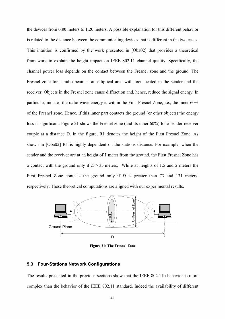
loss is significant. Figure 21 shows the Fresnel zone (and its inner 60%) for a sender-receiver
couple at a distance D. In the figure, R1 denotes the height of the First Fresnel Zone. As
shown in [Oba02] R1 is highly dependent on the stations distance. For example, when the
sender and the receiver are at an height of 1 meter from the ground, the First Fresnel Zone has
a contact with the ground only if D > 33 meters. While at heights of 1.5 and 2 meters the
First Fresnel Zone contacts the ground only if D is greater than 73 and 131 meters,
respectively. These theoretical computations are aligned with our experimental results.
R1
R -
Fres
nel Z
one
Ground Plane
D Figure 21: The Fresnel Zone
5.3 Four-Stations Network Configurations
The results presented in the previous sections show that the IEEE 802.11b behavior is more
complex than the behavior of the IEEE 802.11 standard. Indeed the availability of different

42
transmission rates may cause the presence of several transmission ranges inside the network.
In particular, inside the same data transfer session there may be different transmission ranges
for data and control frame (e.g., RTS, CTS, ACK). Hereafter, we show that the superposition
of these different phenomena makes very difficult to understand the behavior of IEEE
802.11b ad hoc networks. To reduce this complexity, in the experiments presented below the
NIC data rate is set to a constant value for the entire duration of the experiment.10 Hereafter,
we present only the results obtained with the NIC data rate constant, and equal to 11Mbps;
more results can be found in [Ana03].
The four-stations configuration presented in Figure 22 was used in the experiments. The
results obtained are presented in Figure 23.
S1 S2 S3 S4
Session 1 Session 2
25 m 80/85 m 25 m
Figure 22. Network configuration at 11 Mbps.
Figure 23. Throughputs at 11 Mbps.
10 It is worth pointing out that we experienced a high variability in the channel conditions thus making a
comparison between the results difficult.
UDP
0
500
1000
1500
2000
2500
no RTS/CTS RTS/CTS
Thro
ughp
ut (K
bps)
1->2
3->4
TCP
0
500
1000
1500
2000
2500
no RTS/CTS RTS/CTS
Thro
ughp
ut (K
bps)
1->2
3->4
43
These results were the superposition of several factors. In detail, dependencies were observed
between the two connections even though the transmission range was smaller than the
distance between stations S1 and S3. Furthermore, the dependency were observed also when
the basic mechanism (i.e., no RTS/CTS) is used.11 To summarize, this set of experiments
showed that interdependencies among the stations extends beyond the transmission range. To
explain this we hypothesized that all stations were inside the same physical carrier sensing
range, and this produced a correlation between active connections whose effect is similar to
that achieved with the RTS/CTS mechanism (virtual carrier sensing). The difference in the
throughputs achieved by the two sessions when using the UDP protocol (with or without
RTS/CTS) can be explained by considering the asymmetric condition that exists on the
channel: station S2 was exposed to transmissions of station S3 and, hence, when station S1
sent a frame to S2 this station was not able to send back the MAC ACK. Therefore, S1
reacted as in the collision cases (thus re-scheduling the transmission with a larger backoff). It
is worth pointing out that also S3 was exposed to S2 transmissions but the S2’s effect on S3
was less marked given the different role of the two stations. When using the basic access
mechanism, the S2’s effect on S3 was limited to short intervals (i.e., the transmission of ACK
frames). When adopting the RTS/CTS mechanism, the S2 CTS forced S3 to defer the
transmission of RTS frames (i.e., simply a delay in the transmission), while RTS frames sent
by S3 forced S2 to not reply with a CTS frame to S1’s RTS. In the latter case, S1 increased
the back off and rescheduled the transmission. Finally, when the TCP protocol was used the
differences between the throughput achieved by the two connections still existed but were
reduced. The analysis of this case is very complex because we must also take into
consideration the impact of the TCP mechanisms that: i) reduces the transmission rate of the
11 A similar behavior is observed (but with different values) by adopting the RTS/CTS mechanism.

44
first connection, and ii) introduces the transmission of TCP-ACK frames (from S2 and S4)
thus contributing to make the system less asymmetric.
5.4 Physical Carrier Sensing Range
Results presented in the previous section seem to indicate that dependencies among the
stations extend far beyond the transmission range. For example, taking as a reference the
scenario presented in Figure 22, the distance between the two couples of transmitting stations
is about three times the transmission range. The hypothesis is that dependencies are due to a
large physical carrier sensing that includes all the stations. To validate this hypothesis and to
better understand the system behavior we designed some experiments to estimate the physical
carrier sensing range. A direct measure of this quantity seems difficult to achieve because the
802.11b cards we utilized do not provide to the higher layers information about the channel
carrier sensing. Therefore, we defined an indirect way to perform these measurements. We
utilized the scenario shown in Figure 24 with fixed distance between each couple of
communicating stations (d(1,2)=d(3,4)=10 meters), and variable distance between the two
couples, i.e., d(2,3), is variable.
S1 S2 S3 S4
Session 1 Session 2
d(1,2) d(2,3) d(3,4)
Figure 24. Reference network scenario.
The idea is to investigate the correlation among the two sessions while increasing the distance
d(2,3). To measure the correlation degree, just before running each experiment we performed
some preliminary measurements. Specifically, we measured the throughput of each session in
isolation, i.e., when the other session is not active. Then, we measured the throughput of each
session when both sessions are active. Hereafter, Thi(x) denotes the throughput of session i

45
(i=1,2) when both sessions are active and d(2,3)=x. Obviously, Thi(�) denotes the throughput
of session i (i=1,2), when d(2,3)=��� and hence the two sessions are independent. By
exploiting these measurements we estimated the correlation existing between the two sessions
by the following index:
� �)()()()(
121
211
���
�
��
ThThxThxThxD .
The D1(x) index takes the value 0 if the two sessions are independent. Taken a session as a
reference, the presence of the other session may have two possible effects on the performance
of the reference session: 1) if the two sessions are within the same physical carrier sensing
range, they share the same physical channel; 2) if they are outside the physical carrier sensing
range the radiated energy from one session may still affect the quality of the channel observed
by the other session. As the radiated energy may travel over unlimited distances, we can
expect that D1(x) may be equal to zero only for very large distances among the sessions
[Eph02a].
When the D1(x) value is greater than zero, the index does not indicate how strong the
correlation is. To measure this second aspect we introduce the D2(x) index:
D2 x� ��Th1(0) � Th2(0)Th1(x) � Th2(x)
.
D2(x) compares the throughput of the two sessions when they are active at the same time and
d(2,3)=x, with respect to the two-session throughput when all the stations are inside the same
transmission range, i.e., d(2,3)=0. A D2(x) value equal to 1 indicates the maximum correlation
that exists when all stations are in the same transmission range.
By varying the distance d(2,3) we performed several experiments to estimate the above
indexes. The results were obtained with the cards transmission rates set to 2 and 11 Mbps, and
are summarized in Table 7 and Table 8, respectively. As it clearly appears from the tables, the

46
correlation among session is still marked when d(2,3) is less than or equal to 250 meters,
noticeably decreases around 300 meters, and further reduces (but not disappears) when the
inter-session distance is about 350 meters.
Table 7: Throughput values (Card rate =11 Mbps, payload size=512 Bytes)
Throughput of Session 1 Throughput of Session 2 Access
Mechanism Distance
Th1(�) Kbps
Th1(x) Kbps
Th2(�) Kbps
Th2(x) Kbps
D1(x) D2(x)
x=0 2780 1849 2981 1768 0.37 1.00
x=150 1950 1500 2950 2250 0.23 0.96
x=180 2920 2210 3040 1580 0.36 0.95
x=200 2290 1930 3160 2660 0.16 0.78
x=250 2820 1700 3170 2760 0.25 0.81
x=300 2980 2800 3060 2750 0.08 0.65
No
RTS/CTS
x=350 2730 2590 3250 3230 0.03 0.62
From the above results we assume that 250 m is approximately the size of the physical carrier
sensing range. After this distance the correlation among the two sessions is due to the mutual
impact on the channel quality. A set of measurements is currently ongoing to further verify
the exact size of the physical carrier sensing range.
It is worth noting that the physical carrier sensing range is almost the same for the two
different transmission rates. Indeed, the physical carrier sensing mainly depends on two
parameters: the stations’ transmitting power and the distance between transmitting stations.
The rate at which data are transmitted have no significant effect on these parameters.
The results obtained confirm the hypotheses we made in the previous section to justify the
apparent dependencies existing among the two couples of transmitting stations even if the
distance among them is about three times greater than the transmission range.
It is worth noting that the ideal value for D1(0) is 0.5, i.e., each session gets half of the
throughput of the session in isolation. This is not true for CSMA MAC protocol as Th1(0)

47
(Th2(0)) is greater than Th1(�)/2 (Th2(�)/2). This results is caused by a smaller overhead of
the backoff algorithm in the experiments with d(2,3)=0.
Table 8: Throughput values (Card rate =2 Mbps, payload size=512 Bytes)
Throughput Session 1 Throughput Session 2 Access Mechanism
Distance Th1(�) Th1(x) Th2(�) Th2(x)
D1(x) D2(x)
x=0 1279 577 1253 561 0.55 1.00
x=150 1310 880 1310 780 0.37 0.69
x=180 1310 930 1310 820 0.33 0.65
x=200 1270 1030 1330 1130 0.17 0.53
x=250 1300 960 1330 960 0.27 0.59
x=300 1370 1360 1380 1050 0.12 0.47
No
RTS/CTS
x=350 1360 1110 1400 1390 0.09 0.45
5.5 Channel Model for an IEEE 802.11 Ad Hoc Network
The results presented in this paper indicate that for correctly understanding the behavior of an
802.11 network operating in ad hoc mode, several different ranges must be considered.
PCS_RangeTx(1)
Tx(2) Tx(11)S
Tx(5.5)
Radi
ated
Are
a
Figure 25: Channel model for an 802.11 ad hoc network.

48
Specifically, as shown in Figure 25, given a transmitting station S, the stations around will be
affected by the station S transmissions in a different way depending on the distance from S
and the rate used by S for its transmissions.
Specifically, assuming that S is transmitting with a rate x x � 1, 2, 5.5, 11� �� � stations around
it can be partitioned into three classes depending on their distance, d, from S:
i. Stations at a distance d < TX_Range(x) are able to correctly receive data from S, if
S is transmitting at a rate lower or equal to x;
ii. Stations at a distance d, where TX_Range(x) < d < PCS_Range, are not able to
receive data correctly from station S. However, as they are in the S physical carrier
sensing range, when S is transmitting they observe the channel busy and thus they
defer their transmissions.
iii. Stations at a distance d > PCS_Range do not measure any significant energy on the
channel when S is transmitting, therefore they can start transmitting
contemporarily to S; however, the quality of the channel they observe may be
affected by the energy radiated by S. In addition, if d < PCS_Range +
TX_Range(x) some interference phenomena may occur (see below). This
interference depends on the IF_Range value. This value is difficult to model and
evaluate as it depends on several factors (mainly the power at the receiving site)
but as explained before TX_Range(1) < IF_Range < PCS_Range.
Several interesting observations can be derived by taking into consideration points i-iii above.
Firstly, the hidden station phenomenon, as it is usually defined in the literature (see Section
2.2), is almost impossible with the ranges measured in our experiments. Indeed, the
PCS_Range is more than twice TX_Range(1), i.e., the larger transmission range.
Furthermore, two stations, say S1 and S2, that can start transmitting towards the same
receiver, R, must be at a distance ≤ 2•TX_Range(1), and thus they are inside the physical

49
carrier sensing range of each other. Hence, if S1 has an ongoing transmission with R, S2 will
observe a busy channel and thus will defer its own transmission. This means that, in this
scenario, virtual carrier sensing is not necessary and the RTS/CTS mechanism only introduces
additional overhead.
S
R
IF_Range
TX(1)
PCS_
Rang
e
S1
R1
IF_Range
Figure 26 : Interference-based hidden station phenomenon.
While the hidden station phenomenon, as defined in the literature, seems not relevant for this
environment point iii above highlights that packets cannot be correctly received due to the
interference caused by a station that is “hidden” to the sending station. An example of this
type of hidden station phenomenon is presented in Figure 26. In this figure we have two
transmitting stations, S and S1 that are outside their respectively PCS_Range and hence they
are hidden to each other. In addition we assume that the receiver of station S (denoted by R in
the figure) is inside the interference range (IF_Range) of station S1. In this scenario S and S1
can be simultaneously transmitting and, if this occurs, station R cannot receive data from S
correctly. Also in this case the RTS/CTS mechanism does not provide any help and new
50
coordination mechanisms need to be designed to extend the coordination in the channel
access beyond the PCS_Range.
It is worth noting that, in our channel model, the exposed station definition (see Figure 6)
must be modified too. In this scenario, exposed stations are those station at a distance
PCS_Range- TX_Range(1) < d < PCS_Range. Indeed, these stations are exposed to station S
transmissions, while they are in the transmission range of stations with d > PCS_Range . The
following example outline problems that may occur in this case. Let us denote with S1 a
station at a distance d from S: PCS_Range < d < PCS_Range+TX_Range(x). Station S1 can
start transmitting, with a rate x, towards a station E that is inside the physical carrier sensing
of S; station E cannot reply because it observes a busy channel due to the ongoing station S
transmissions, i.e., E is exposed to station S. Since station S1 does not receive any reply
(802.11 ACK) from E, it assumes an error condition (collision or CRC error condition), hence
it backoffs and then tries again. If this situation repeats for several times (up to 7), S1 assumes
that E is not anymore in its transmission range, gives up the transmission attempt and
(wrongly) signals to the higher layer a link breakage condition, thus forcing higher layers to
attempt a recovery action (e.g., new route discovery, etc. – see Section 3).
To summarize, results obtained in the configuration we analyzed indicate that the hidden
station and exposed station definitions must be extended. These new hidden-station and
exposed-station phenomena may produce undesirable effects that may degrade the
performance of an ad hoc network, mainly if the TCP protocol is used. Extending the
coordination in the channel access beyond the PCS_Range seems to be the correct direction
for solving the above problems.

51
5.6 The Communication Gray Zones Problem
An important problem related to the different transmission ranges of control and data frames
is the so-called communication gray zones problem [Lun02]. This problem was revealed by a
group of researchers at the Uppsala University. While measuring the performance of a their
own implementation of the AODV routing protocol [Per99] in an IEEE 802.11b ad hoc
network, they observed an unexpected large amount of packets’ losses, especially during
route changes. They found that the increase in packet loss occurred in some specific
geographic areas that they called “communication gray zones”. In such zones the packet loss
experienced by a station may be extremely high, up to 100%, thus severely affecting the
performance of those applications characterized by a continuous packet flow (e.g., file
transfers and multimedia streaming). They also found that the ultimate reason for this
phenomenon is that a station inside a gray zone is considered as reachable by a neighboring
station, based on its routing information, but data communication between the stations is not
possible. The same problem was found to affect other routing protocols like OLSR [Cla02]
and LUNAR [Tsc02].
To better understand why communication gray zones arise it is worthwhile to briefly recall
how the AODV routing protocol works. AODV is a reactive protocol that discovers and
maintains routes on demand. When a route to a target station is needed, the AODV protocol
broadcasts a route-request message that is then disseminated throughout the network. When
the target station (or a valid route to the target station) is found, a route-reply message is sent
back to the requesting station by means of a unicast message. While this message travels
towards the requesting station, routes are set up inside routing tables of the traversed stations.
In addition to the request-reply mechanism, the AODV protocol uses a sensing mechanism to
discover neighboring stations and, based on this, to update, add or remove routes in the
routing table. Periodically, each station broadcasts HELLO beacons. Upon reception of an

52
HELLO message from a neighboring, a station becomes aware that the neighboring station is
reachable and can, thus, be used to relay data transmissions. Routing table are, thus, updated
accordingly.
Several elements contribute to the occurrence of communication gray zone. In particular, the
different properties of HELLO messages with respect to data messages play an important role.
These properties, and their effects, are summarized below.
1. Transmission rate. Since HELLO beacons are broadcast messages they are transmitted
at the basic rate (2 Mbps). On the other hand, data packets (that are unicast) may be
transmitted at 11 or 5.5 Mbps. Therefore, HELLO messages have a transmission range
larger than data messages.
2. No Acknowledgement. In 802.11b broadcast messages are transmitted without
acknowledgement. Therefore, a station that receives an HELLO message from a
neighboring has no indication whether transmission is possible even in the opposite
direction, i.e., there is no indication that the link is bi-directional.
3. Packet size. In general, HELLO messages are much smaller in size than data packets.
As is well known, small packets have a lower probability to be affected by
transmission errors, and minor chances of colliding with other packets. Therefore, it is
more likely for an HELLO message to reach a receiver than a data packet, especially
when the link quality is poor.
In addition to the above elements, the effects of fluctuating links need to be taken into
account, as well. At the border of the transmission range the communication quality tends to
be fluctuating. In such conditions it may happen that a station sporadically receives an HELLO
message from a neighbor, but this does not imply that consistent communication between the
stations is actually possible. Since the AODV protocol updates routing tables based on the

53
neighboring sensing mechanism (i.e., based on the reception of HELLO message) it may occur
that stable and longer routes are replaced by shorter but unreliable ones.
MS
FS2FS1GW
Brodcast Range
Unicast Range
Gray Zone
Figure 27. A scenario where communication gray zones can be experienced (taken from [Lun02]).
Figure 27 depicts a scenario pointed out by the researchers at Uppsala University where
communication gray zone can be experienced by the mobile station MS (see [Lun02]). In this
scenario, stations labeled as GW, FS1 and FS2 are static, while station MS moves forward
and back as indicated in the figure. There is an active communication between the gateway
Station GW and the mobile station MS. Depending on the physical position of the mobile
station, the traffic from MS to GW (and vice-versa) is routed trough one, two or three hops
via intermediate stations FS1 and FS2. Theoretically, the MS has always a route towards GW.
However, while moving from the initial position to the rightmost position MS will pass
through two gray zone. Similarly, two gray zones will be traversed in the reverse path. In
[Lun02] it is shown that traversal of the gray zones are associated with time intervals during
which MS experience a packet loss of up to 100%. The duration of this time interval, as well
as the peak value in the packet loss experienced by the mobile station, depends on the specific
routing protocol.
Before proceeding on it is important to highlight that communication gray zone problem can
not be revealed by using the current simulation tools (e.g., ns-2). Indeed, in the IEEE 802.11
model implemented by simulation tools both unicast and broadcast transmissions are
performed at 2 Mbps and, hence, they have the same transmission range. Furthermore,

54
connectivity is modeled as on/off, i.e., the communication becomes impossible as soon as the
distance exceeds the transmission range.
In [Lun02] the authors also propose some possible solutions for alleviating the
communication gray zones problem, namely: (i) the exchange of the neighboring set (i.e.,
stations include their neighboring set in HELLO messages); (ii) the transmission of N-
consecutive HELLO messages; and (iii) the introduction of a SNR threshold to discard weak
control messages. They have also assessed, by means of an experimental analysis, that the
SNR-threshold approach is the most effective and it eliminates the effects of communication
gray zones almost completely.
6. Evolution of IEEE 802.11b for Ad Hoc Networks
In ad hoc networks each station logically operates similarly to a router. However, from the
physical standpoint, there is a significant difference between a router and a station in an ad
hoc network. Typically, a router has multiple network interfaces, and a packet received from
one interface is retransmitted through a different interface (see the left side of Figure 28). On
the other hand, in a multi-hop ad hoc network a station has a single wireless interface and
packets are received from and transmitted through the same interface (see the right side of
Figure 28).
BA
R ABR
Figure 28. Packet forwarding in a router in a wired network (left) and in ad hoc networks (right).
Current ad hoc network architectures do not take into account this difference, and implement
in ad hoc stations the same functionalities of a router. Specifically, packets received from the

55
wireless medium are delivered to the IP layer where a route lookup is performed based on the
destination IP address (steps 1-3 in Figure 29-left). If the packet is not destined to the station
itself it is passed down to the network interface to be retransmitted (steps 4 and 5 in Figure
29-left).
The difference, from the forwarding standpoint, between an ad hoc station and a router has
been recently pointed out by A, Acharya et. alt. who have also proposed an architecture for
efficient packet forwarding at stations in multi-hop ad hoc networks [Ach02].
NIC
IPLayer
Bus
Host
1
2
3
4
5
NIC
Bus
Host
12
3
Figure 29. Forwarding in ad hoc stations: legacy approach (left) and NIC based forwarding (right).
The first question addressed in [Ach02] is which is the best architecture for forwarding a
packet in ad hoc networks. The answer is highlighted in Figure 29. The left-hand side in the
figure depicts the legacy approach for forwarding packets, while the right-hand side shows the
new approach proposed by the authors. In the latter case, the forwarding is completely
managed by the network interface card (NIC). Upon receiving a packet, the NIC (by
exploiting some local information) determines whether or not the packet has to be
retransmitted. Only packets destined to the station itself are passed to higher-level protocols.
Due to its behavior the proposed architecture has been named Cut-through architecture
[Ach02].
The Cut-through architecture provides several advantages that can be classified into two
categories. The first category includes advantages that are not related to a specific MAC

56
protocol, while advantages belonging to the second category are strongly related to the
random access scheme and the RTS-CTS mechanism used in the IEEE 802.11 MAC protocol.
The following advantages belong to the first category:
a) The NIC does not need to interrupt the CPU for packet processing. This could lead to
a considerable power saving for example, if the station is used only for packet
forwarding purposes. The CPU needs to wake up only for processing route updates.
b) Delays for transferring data from the NIC to the host and vice-versa are avoided.
c) Local traffic does not further delays forwarding traffic. In legacy IEEE802.11
architecture, at the forwarding station, the packet is transferred to the main memory by
the NIC. The host CPU is notified (e.g. via interrupts) for further processing of the
packet by the IP protocol stack running on the host CPU. The host software (IP
protocol stack) would typically queue up the packet in a transmission queue (together
with the locally generated packets) and select packets for transmission based on a
scheduling algorithm (typically, FIFO). Thus packets generated by applications
running at the station can overtake packets to be forwarded. This produces an increase
in the end-to-end delay.
As the other advantages are strictly related to the IEEE 802.11 MAC protocol they can be
better understood by first considering the operations performed at the MAC layer by stations
A, B and R in the scenario depicted in the right side of Figure 28.
6.1 Forwarding Operation: Legacy approach vs. NIC-based approach
Let us consider the case shown in Figure 30, where A is the upstream station, R is the
forwarding station, and B the downstream station. In the legacy approach, the data delivery
from A to B involves two separate and independent transmissions. For each transmission the
IEEE 802.11 MAC protocol (including the RTS/CTS mechanism) is used.

57
ACK
SIFS
DATA
SIFS
RTSA
R
B
A and R can access the channelNAV DATA
NAV CTSNAV RTS
The other stations must defer the medium access
CTS
SIFS
A to R transmission
RTS
CTS
SIFS
DATASIFS
ACK
ContentionDIFS
ContentionDIFS SIFS
NAV DATANAV CTS
NAV RTS
R and B can access the channelThe other stations must defer the medium access
R to B transmission
Node Processing
Figure 30. Forwarding operations in the legacy approach.
Specifically, with reference to Figure 30, the transmission from A to R is first performed. At
R the packet is passed to the IP protocol, processed by the IP software, and passed down to
the NIC for transmission to B. A this time, R has to repeat the same procedure executed by A
during the transmission to R. Note that the two transmissions (from A to R, and from R to B)
are independent each other from the channel access standpoint.
It is worth noting that, after the first RTS/CTS exchange, stations A and R got the channel
control and no other station in the transmission range of A and/or R can access the channel.
However, this control is immediately lost after the ACK transmission from R to A. Clearly,
from the Station R standpoint, it is not very wise to release the channel control, and
immediately after compete again for gaining the channel control. It would be better for R to
maintain the exclusive control on the channel. In this case the transmission to B would be
done without contention, thus improving the bandwidth utilization (there would be no
bandwidth wastage due to collisions and backoff periods), and minimizing the forwarding
delay. Obviously, Station R should operate the packet forwarding very quickly so that the
transmission from R to B could start immediately after the ACK transmission from R to A.
This can be achieved only if the forwarding operation is performed completely inside the NIC
(right-hand side of Figure 29).

58
Figure 31 shows an extension of the IEEE 802.11 MAC protocol to manage packet
forwarding in a more efficient way [Ach02]. The basic idea is to give the highest priority to
the traffic to be forwarded by extending the channel reservation scheme to allow on-the-fly
transmissions. Specifically, upon receiving a frame from A, Station R not only sends back an
ACK frame to A but, at the same time, it transmits an RTS frame to further extend the
channel reservation.12 Since the RTS frame transmission occurs while all the other stations
within the R’s transmission range are still blocked (due to the previous RTS/CTS exchange)
station R can immediately get the channel. The extended MAC protocol has been named
Data-driven Cut-through Multiple Access (DCMA).
ACK
SIFS
DATA
SIFS
RTS
ContentionDIFS
A
R
B
A and R can access the channelNAV DATA
NAV CTSNAV RTS
The other stations must defer the medium access
CTS
SIFS
RTS
CTS
SIFS
SIFS
DATASIFS
ACK
NAV DATANAV CTS
NAV RTS
R and B can access the channel
A to R transmission
R to B transmission
Figure 31. Forwarding operations in the NIC-based approach.
6.2 DCMA MAC protocol
The DCMA MAC protocol is an extension of the IEEE 802.11 DCF and, as such, it follows
the associated 4-way handshake involving the exchange of RTS/CTS/DATA/ACK frames. As
shown in the previous section, the DCMA attempts to replace the two distinct channel
accesses (upstream and downstream) with a combined access. Specifically, DCMA combines
the ACK (to the upstream station) with the RTS (to the downstream station) in a single
ACK/RTS packet that is sent to the MAC broadcast destination address.
12 More precisely, the RTS frame is piggybacked to the ACK frame.
59
The cut-through approach, proposed in DCMA, fails when the downstream station (e.g., B in
our example) cannot reply to the ACK/RTS (with a positive CTS). In such a case the
forwarding station then simply queues the packet in the NIC queue, and resumes the normal
IEEE 802.11 channel access method using the exponential backoff to regulate subsequent
access to the shared channel. The channel contention resolution of DCMA is same as that of
802.11, with a station remaining silent as long as any of its one-hop neighbors are either
receiving or transmitting a data packet. Accordingly, this protocol does not suffer from any
additional penalties, over and above those present in 802.11.
Since DCMA has no notion of future reservations (all access attempts are for immediate
transfer of DATA frames), it does not require any modifications or enhancements to the
802.11 NAV—a station simply stays quiet as long as it is aware of (contiguous) activity
involving one or more of its neighbours. Any station that overhears an ACK/RTS not
addressed to it merely increments the NAV by the time interval included in the ACK/RTS
message.
In [Ach02] a simulation analysis of the DCMA scheme is also presented. This analysis was
carried out by implementing the DCMA access protocol in the ns-2 simulation tool.
Consequently, the ns-2 typical values were used: bit rate of 2 Mbps, transmission range equal
to 250 m, and interfering range equal to 550 m. All transmissions, regardless of the frame
size, were preceded by an RTS/CTS exchange.
In the simulation study, high-rate sources were used to guarantee a never empty queue at the
transmitter. To avoid the interference of TCP mechanisms, UDP protocol was used at the
transport layer. The statistics were estimated by considering only the packets correctly

60
received at the receiver. In the forwarding stations routing tables13 were pre-configured with
the shortest path routes to their respective destinations.
Table 9. Throughput comparison (in Kbps).
Packet size (Bytes)
256 512 1024 1536
802.11 159 200 231 258
DCMA 197 242 282 301
Table 10. End-to-end delay comparison (in sec).
Packet size (Bytes)
256 512 1024 1536
802.11 1.00 1.67 2.59 2.83
DCMA 0.50 0.81 1.31 1.73
Several configurations are considered in [Ach02]. For the sake of space only a set of them are
discussed here. They refer to a string or chain topology (see Figure 8) where the distance
between successive stations is 250 m. A single flow of UDP packets is transmitted from the
leftmost to the rightmost station. Several experiments were conducted by varying the size of
the payload from 256 to 1536 bytes.
The results obtained by considering a 7-hop chain are summarized in Table 9 and Table 10. It
clearly appears that DCMA improves the throughput around 20% with respect to the standard
13 The contents of these routing tables will be briefly discussed in the following. A complete description can be
found in [Ach02].

61
protocol, while the delay improvement is more significant, ranging from 63% (1536bytes) to
100% (256byte packets).
In [Ach02] the comparison was further extended by considering an increasing number of hops
in the chain. The results obtained are consistent with results presented in Table 9 and Table
10: the delay reductions with DCMA are significant (in the order of 50%), while throughput
improvements are marginal.
Table 11.Throughput (in Kbps) as a function of the offered load.
Offered Load (Kbps)
250 275 300 325 350 375 400 425 450 475 500
802.11 242 267 292 316 340 364 259 273 256 241 235
DCMA 242 267 292 316 340 364 389 413 376 376 374
Table 12. End-to-end delay (in sec) as a function of the offered load.
Offered Load (Kbps)
250 275 300 325 350 375 400 425 450 475 500
802.11 0.075 0.075 0.075 0.075 0.075 0.075 0.075 0.075 0.75 0.95 1.09
DCMA 0.080 0.080 0.080 0.080 0.080 0.080 1.37 1.53 2.06 2.02 2.08
Finally the influence of the offered load was considered. The results obtained are summarized
in Table 11 and Table 12. Specifically, these results are related to a 12-hop chain and have
been obtained by increasing the sending rate at the source from 250 Kbps to about 500 Kbps.
It clearly appears that there is a different saturation points for the two protocols. The IEEE
802.11 MAC protocol has the maximum throughput at around 0.375 Mbps; after this offered
load level the queues start to build up, the end-to-end delay has a significant increase and the

62
throughput decreases. On the other hand, DCMA has the maximum throughput at around
0.425 Mbps. Furthermore, after the saturation point DCMA shows a more stable behavior: the
throughputs remains high, and the end-to-end delay is about half that of the standard protocol.
Acknowledgements
This work was funded partially by the Information Society Technologies programme of the European Commission, Future and Emerging Technologies under the IST-2001-38113 MobileMAN project, and partially by the Italian Ministry for Education and Scientific Research in the framework of the FIRB-VICOM project. The authors wish to express their gratitude to Veronica Vanni, Eleonora Borgia and Riccardo Bettarini for performing the experiments discussed in this chapter.
References
[Ach02] A. Acharya, A. Misra, S. Bensal, “A Label-switching Packet Forwarding Architecture for Multi-hop Wireless LANs”, Proceedings of the ACM Workshop on Mobile Multimedia (WoWMoM 2002), Atlanta (GA), September 28, 2002.
[Ahu00] A. Ahuja et al., “Performance of TCP over different routing protocols in mobile ad-hoc networks,” Proceedings of the IEEE Vehicular Technology Conference (VTC 2000), Tokyo, Japan, May 2000.
[Ana03] G. Anastasi , E. Borgia, M. Conti, E. Gregori, “IEEE 802.11 Ad Hoc Networks: Performance Measurements”, Proceedings of the Workshop on Mobile and Wireless Networks (MWN 2003), Providence (Rhode Island), May 19, 2003.
[Cha01] K. Chandran, S. Raghunathan, S. Venkatesan, R. Prakash, “A Feedback Based Scheme for Improving TCP Performance in Ad Hoc Wireless Networks”, IEEE Personal Communication Magazine, Special Issue on Ad Hoc Networks, Vol. 8, N. 1, pp. 34-39, February 2001.
[Cla02] T. Clausen and al., “Optimized Link State Routing Protocol”, Internet Draft, IETF MANET Working Group, November 2002, available at http://menetou.inria.fr/olsr/draft-ietf-manet-olsr-07.txt.
[Dye01] T.D. Dyer, R.V. Boppana “A Comparison of TCP Performance over Three Routing Protocols for Mobile Ad Hoc Networks”, Proceedings of the ACM Symposium on Mobile Ad Hoc Networking & Computing (MobiHoc), October 2001.
[Eph02] T. Ephremides, “A Wireless Link Perspective in Mobile Networking", ACM Mobicom 2002 keynote speech, available at http://www.acm.org/sigmobile/mobicom/2002/program/
[Eph02a] T. Ephremides, “Energy Concerns in Wireless Networks”, IEEE Wireless Communications, August 2002, pp. 48-59.
[FuM02] Z. Fu, X. Meng, S. Lu, “How Bad TCP Can Perform in Mobile Ad Hoc Networks”, Proceedings of the IEEE Symposium on Computers and Communications (ISCC 2002), Taormina-Giardini Naxos (Italy), July 2002, pp. 298-303.
[Fu03] Z. Fu, P. Zerfos, K. Xu, H. Luo, S. Lu, L. Zhang, M. Gerla, “The Impact of Multihop Wireless Channel on TCP Throughput and Loss“, Proceedings of IEEE INFOCOM 2003, San Francisco (CA), March 30 – April 3, 2003.
[Glo] GloMoSim, Global Mobile Information Systems Simulation Library,

63
http://pcl.cs.ucla.edu/projects/glomosim/.
[Hol99] G. Holland, N. Vaidya, “Analysis of the TCP Performance over Mobile Ad Hoc Networks”, Proceedings of the ACM International Conference on Mobile Computing and Networking (MobiCom’99), Seattle (WA), August 1999, pp. 207-218.
[Hol02] Gavin Holland, Nitin H. Vaidya “Analysis of TCP Performance over Mobile Ad Hoc Networks”, ACM/Kluwer Journal of Wireless Networks 8(2-3), (2002) pp. 275-288.
[IEE02] Official Homepage of the IEEE 802.11 Working Group, http://grouper.ieee.org/groups/802/11/.
[IEE99] IEEE standard 802.11, “Wireless LAN Medium Access Control (MAC) and Physical Layer (PHY) Specifications, August 1999.
[Li01] J. Li, C. Blake, D. De Couto, H. Lee, R. Morris, “Capacity of Wireless Ad Hoc Wireless Networks”, Proceedings of the ACM International Conference on Mobile Computing and Networking (MobiCom’01), Rome (I), July 2002, pp. 61-69.
[Liu01] J. Liu, S. Singh, “ATCP: TCP for mobile ad hoc networks”, IEEE Journal on Selected Areas in Communications (J-SAC), 19(7):1300-1315, July 2001.
[Lun02] H. Lundgren, E. Nordstron, C. Tschudin, “Coping with Communication Gray Zones in IEEE 802.11 based Ad Hoc Networks”, Proceedings of the ACM Workshop on Mobile Multimedia (WoWMoM 2002), Atlanta (GA), September 28, 2002, pp. 49-55.
[Mon00] J.P. Monks, P. Sinha, V. Bharghavan, “Limitations of TCP-ELFN for Ad Hoc Networks”, Proceedings of MoMuc 2000, Tokyo, Japan, October 2000.
[Ns02] The Network Simulator - ns-2, http://www.isi.edu/nsnam/ns/index.html.
[Oba02] Mohammad S. Obaidat, David G. Green, “An Accurate Line of Sight Propagation Performance Model for Ad Hoc 802.11 Wireless LAN (WLAN) Devices”, Proc. ICC 2002, New York City, April 28 – May 2, 2002.
[Per99] C. Perkins, E. Royer, “Ad Hoc On-Demand Distance Vector Routing”, Proceedings of the 2nd IEEE Workshop on Mobile Computing Systems and Applications (WMCSA’99), February 1999.
[Qua02] Qualnet simulator, http://www.qualnet.com/.
[Tan99] K. Tang, M. Gerla, “Fair Sharing of MAC under TCP in Wireless Ad Hoc Networks”, Proceedings of IEEE MMT’99, Venice (I), October 1999.
[Tsc02] C. Tschudin, R. Gold, “LUNAR: Lightway Underlay Network Ad Hoc Routing”, available at http://www.docs.uu.se/docs/research/projects/selnet/lunar/lunar.pdf.
[XuS01] S. Xu and T. Saadawi, “Does the IEEE 802.11 MAC protocol Work Well in Multihop Wireless Ad Hoc Networks?”, IEEE Communication Magazine, Volume 39, N. 6, June 2001, pp. 130-137.
[XuS02] S. Xu and T. Saadawi, “Revealing the Problems with 802.11 MAC Protocol in Multi-hop Wireless Networks”, Computer Networks, Volume 38, N. 4, March 2002.
[XuB02] K. Xu, S. Bae, S. Lee, M. Gerla, “TCP Behavior across Multihop Wireless Networks and the Wired Networks”, Proceedings of the ACM Workshop on Mobile Multimedia (WoWMoM 2002), Atlanta (GA), September 28, 2002, pp. 41-48.
[XuG02] K. Xu, M. Gerla, “TCP over an IEEE 802.11 Ad Hoc Network: Unfairness Problems and Solutions”, UCLA Computer Science Deptartment Technical Report – 020019, May 2002.
[Zar03] G. Zaruba, S. Das, “Off-the-Shelf Enablers of Ad Hoc Networks“, in Mobile Ad hoc networking, S. Basagni, M. Conti, S. Giordano, I. Stojmenovic (Editors), IEEE Press and John Wiley and Sons, Inc., New York, 2003.