EET/2003/03

IEA/EET Working Paper

APPLYING PORTFOLIO THEORY TOEU ELECTRICITY PLANNING AND

POLICY-MAKING

Shimon Awerbuch with Martin Berger

February 2003

The views expressed in this Working Paper are those of the authorsand do not necessarily represent those of the IEA or IEA policy.Working Papers describe research in progress by the authors and arepublished to elicit comments and to further debate.

2EET/2003/03

Report Number EET/2003/03Paris, February 2003

APPLYING PORTFOLIO THEORY TO EUELECTRICITY PLANNING AND POLICY-MAKING

Shimon AwerbuchMartin Berger

Abstract

���� ������ �������� � � ����� ����� �� ����� ���� ������ ��� ���� ���������� � �� ��� �� ����������������� �������������������������������������� �������������� ������������ �������� ����������������� ������� �������������������!!� ���� ��������������� ����

Shimon Awerbuch: s.awerbuch@sussex.ac.ukMartin Berger: berger@risc.iew.tuwien.ac.at

International Energy Agencywww.iea.org

This study presents an effort to apply one of the well-known elements of modern finance theory tothe process of evaluating generating technologies and generating portfolios: Mean-VariancePortfolio Theory. The underlying motive for the study is a perception that there has been onlylimited understanding to date of how improved (that is, efficient or optimal) energy portfolios mightbe constructed by applying modern mean-variance portfolio theory. The result of the study is that aportfolio of energy technologies with differing financial characteristics could be less costly, overtime, than a portfolio constructed exclusively from fuel-based systems.

3EET/2003/03

APPLYING PORTFOLIO THEORY TO EUELECTRICITY PLANNING AND POLICY-MAKING

OVERVIEW OF THIS REPORT

This study, co-authored by Shimon Awerbuch and Martin Berger, introduces mean-variance portfoliotheory and evaluates its potential application to the development of efficient (optimal) European Union(EU-15) generating portfolios that enhance energy security and diversification objectives. Theanalysis extends to European countries the previous work done by Awerbuch in the US, and applies asignificantly more detailed portfolio model that reflects the risk of the relevant generating coststreams: fuel, operation and maintenance (O&M) and construction period costs. It illustrates theportfolio effects of different generating mixes. The study offers preliminary findings on the effects ofincluding more renewable energy sources in the typical EU portfolio mix and suggests interestingdirections for further study.

The study arises from the perception that these standard, finance-oriented analyses may offer valuableenhancements to energy planning, and concepts of energy security and diversity. Clearly thecombination of better portfolio construction and more accurate pricing should lead to more optimaldecisions in the round. This study, therefore, represents an effort to complement traditional approachesand point researchers and planners into new territory.

Author’s Acknowledgements

This study was prepared in the Renewable Energy Unit of the Energy Technology Division.Thanks to Dr. Hanns-Joachim Neef, Head, Technology Collaboration Division, Mr. RichardSellers, Head, Renewable Energy Unit and my REU colleagues, especially Mark Hammonds andSebastian Linnemayr. I also thank Dr. Roberto Vigotti and the members of IEA’s RenewableEnergy Working Party for their encouragement and support of this work.

This study would not have been possible without the Swedish Government, whose financialsupport I gratefully acknowledge, along with the efforts of Ms. Yvonne Fredrickson and Mr. LarsGuldbrand of the Swedish Ministry of Industry, Employment and Communications. For the study,I was ably assisted by Martin Berger, who was supported by the Austrian Bundesministerium fürVerkehr, Innovation und Technologie. Thanks to that Ministry and Dr. Martin Huemer. I alsoacknowledge the USDOE and the Interstate Renewable Energy Council who have encouraged andsupported my research on the valuation of energy technologies over the last two decades.

Thanks too, to Andrew Freeman who provided substantial editorial re-working of the material andSally Wilkinson who assisted with formatting and proof reading.

Finally, I thank Morgan Stanley, particularly Mr. Vezen Wu of its New York City office and Ms.Helene Denis of its office in Paris for providing the MCSI financial market data used in developingthe fossil fuels risk estimates discussed in Chapter 5.

4EET/2003/03

APPLYING PORTFOLIO THEORY TO EUELECTRICITY PLANNING AND POLICY-MAKING

1.1 Introduction

Portfolio analysis is widely used by financial investors to create robust portfolios that produce efficient

outcomes under various economic conditions. In essence, an efficient portfolio takes no unnecessary

risk relative to its expected return. Put another way, efficient portfolios are defined by the following

properties: they maximise the expected return for any given level of risk, while minimising risk for

every given level of expected return.

In the case of energy policy, portfolio-based techniques can suggest ways to develop diversified

generating portfolios with known risk levels that are commensurate with their expected overall

electricity generation costs. Simply put, the underlying insight is that efficient generating portfolios

can minimise society’s energy price risk.

Energy security considerations1 are generally focused on the threat of abrupt supply disruptions,

although a case can also be made for the inclusion of a second aspect: the risk of unexpected electricity

cost increases. This is a subtler, but equally crucial, aspect of energy security. Energy security is

reduced when countries (and individual firms) hold inefficient portfolios that are needlessly exposed to

cost risk.

A growing body of literature now indicates that fossil price fluctuations depress economic activity in

fossil fuel-importing nations. Even small percentage increases in fossil prices can yield sizeable

economic losses through unemployment and lost income, as well as the loss of value for financial and

other assets.2 Efficient generating portfolios minimise national exposure to such fluctuations,

commensurate with creating optimal overall generating costs. Efficient generating portfolios expose

society to the minimum level of risk needed to attain given energy cost objectives.

Traditional energy planning in the US and Europe focuses on finding the least cost generating

alternative, although in today’s dynamic environment it is probably impossible correctly to identify the

30-year "least cost" option. Least cost procedures are roughly analogous to trying to identify

1 See e.g. Green Paper “Towards a European strategy for the security of energy supply” (European Community

2001).

2 Given the estimates in this literature, such economic losses can run to the tens, even hundreds, of billions of US

dollars: see Sauter and Awerbuch (2002). For an excellent recent survey of this literature see: Papapetrou (2001);see also Sadorsky (1999), Yang, et al. (2002), and Ferderer (1996).

5EET/2003/03

yesterday’s single best performing stock and investing in it exclusively for the next 30 years

[Awerbuch 2000a]. Clearly, modern finance theory offers better tools.

Energy planning is not unlike investing in financial securities, where financial portfolios are widely

used by investors to manage risk and to maximize performance under a variety of unpredictable

outcomes. Similarly, it is important to conceive of electricity generation not in terms of the cost of a

particular technology today, but in terms of its portfolio cost. At any given time, some alternatives in

the portfolio may have high costs while others have lower costs, yet over time, an astute combination

of alternatives can serve to minimize overall generation cost relative to the risk.

Energy planning needs to focus less on finding the single lowest cost alternative and more on

developing efficient (i.e. optimal) generating portfolios. Indeed, modern finance theory would counsel

us to evaluate the relative cost of conventional and renewable energy sources not on the basis of their

stand-alone cost, but on the basis of their portfolio cost –– i.e. their cost contribution relative to their

risk contribution to a portfolio of generating resources. More precisely, the relevant portfolio measure

for valuing generating options is how a particular option affects the generating costs of the portfolio of

resource options relative to how it affects the risk of that portfolio.

Along these lines, it can be shown (Awerbuch, 2000, 1995b) that adding wind, PV and other fixed-cost

renewables to a portfolio of conventional generating assets serves to reduce overall portfolio cost and

risk, even through their stand-alone generating costs may be higher. The important implication of

portfolio-based analysis is that the relative value of generating assets must be determined not by

evaluating alternative resources, but by evaluating alternative resource portfolios.

This analysis focuses on the EU and makes some substantial enhancements to a portfolio model first

used by Awerbuch to evaluate the US gas-coal generation mix [Awerbuch (2000), Awerbuch (1995b)].

That model considered only fuel price risk of two technologies, on the presumption that for fossil

technologies fuel costs dominate other cost categories and therefore provide a reasonable mean-

variance proxy. The current model, by contrast, appropriately defines fuel, O&M, as well as

construction period risk on the basis of the historic standard deviation (SD) of their “holding period”

returns and their interrelationship (covariance) with other costs. In addition, the current model handles

a full complement of technologies including gas, coal, nuclear, oil and a “bundle” of renewables

represented in this analysis by wind technology.

6EET/2003/03

Portfolio basics 3

Portfolio selection is generally based on mean-variance portfolio theory developed by Harry

Markowitz (1952). It enables the creation of minimum-variance portfolios for any given level of

expected (mean) return. Such efficient portfolios therefore minimise risk, as measured by the standard

deviation (SD) of periodic returns.4 The idea is that while investments are unpredictable and risky, the

co-movement or covariance of returns from individual assets can be used to help insulate portfolios,

thus creating higher returns with little or no additional risk.

Portfolio theory was initially conceived in the context of financial portfolios, where it relates E(rp), the

expected5 portfolio return, to σp, the total portfolio risk, defined as the standard deviation of past

returns.6 The relationship is illustrated below using a simple, two-stock portfolio. The expected

portfolio return, E(rp), is the weighted average of the individual expected returns E(ri) of the two

securities:

E(rp) = X1•E(r1) + X2•E(r2) (1.1)

Where:

E(rp) is the expected portfolio return;

X1, X2 are the proportions (percentages) of the assets 1 and 2 in the portfolio; and

E(r1), E(r2) are the expected returns for assets 1 and 2; specifically: the mean of all possible

outcomes, weighted by the probability of occurrence; e.g.: for asset 1 it can be written:E(r1) = ∑piri where pi is the probability that outcome i will occur, and ri is the return

under that outcome.

Portfolio risk, σp, is also a weighted average of the two securities, but is tempered by the correlation

coefficient between the two returns:

2112212

22

22

12

1 2 σσρσσσ XXXXp ++= (1.2)

3 Parts of this section previously appeared in Awerbuch (1995b) and Awerbuch (2000).

4 The standard deviation is simply the square root of variance.

5 In the case of perfect markets, expectations are assumed to be unbiased, but not error-free.

6 Financial holding period return [Seitz (1990) p. 225]:

t

tttt BV

CFBVEVr

+−= where EVt is the ending value,

BVt the beginning value and CFt the “cash inflow during each period t”. It is assumed that the past is a guide tothe future.

7EET/2003/03

Where:

ρ12 is the correlation coefficient between the two return streams7, and

σ1 and σ1 are the standard deviations of the periodic returns to asset 1 and 2 respectively.

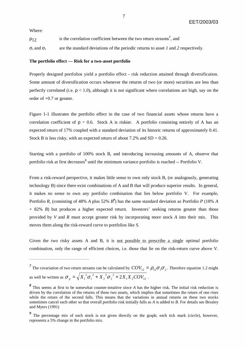
The portfolio effect — Risk for a two-asset portfolio

Properly designed portfolios yield a portfolio effect - risk reduction attained through diversification.

Some amount of diversification occurs whenever the returns of two (or more) securities are less than

perfectly correlated (i.e. ρ < 1.0), although it is not significant where correlations are high, say on the

order of +0.7 or greater.

Figure 1-1 illustrates the portfolio effect in the case of two financial assets whose returns have a

correlation coefficient of ρ = 0.6. Stock A is riskier. A portfolio consisting entirely of A has an

expected return of 17% coupled with a standard deviation of its historic returns of approximately 0.41.

Stock B is less risky, with an expected return of about 7.2% and SD = 0.26.

Starting with a portfolio of 100% stock B, and introducing increasing amounts of A, observe that

portfolio risk at first decreases8 until the minimum variance portfolio is reached -- Portfolio V.

From a risk-reward perspective, it makes little sense to own only stock B, (or analogously, generating

technology B) since there exist combinations of A and B that will produce superior results. In general,

it makes no sense to own any portfolio combination that lies below portfolio V. For example,

Portfolio R, (consisting of 48% A plus 52% B9) has the same standard deviation as Portfolio P (18% A

+ 82% B) but produces a higher expected return. Investors’ seeking returns greater than those

provided by V and R must accept greater risk by incorporating more stock A into their mix. This

moves them along the risk-reward curve to portfolios like S.

Given the two risky assets A and B, it is not possible to prescribe a single optimal portfolio

combination, only the range of efficient choices, i.e. those that lie on the risk-return curve above V.

7 The covariation of two return streams can be calculated by 211212 σσρ=COV . Therefore equation 1.2 might

as well be written as 12212

22

22

12

1 2 COVXXXXp ++= σσσ .

8 This seems at first to be somewhat counter-intuitive since A has the higher risk. The initial risk reduction is

driven by the correlation of the returns of these two assets, which implies that sometimes the return of one riseswhile the return of the second falls. This means that the variations in annual returns on these two stockssometimes cancel each other so that overall portfolio risk initially falls as A is added to B. For details see Brealeyand Myers (1991)

9 The percentage mix of each stock is not given directly on the graph; each tick mark (circle), however,

represents a 5% change in the portfolio mix.

8EET/2003/03

Investors will choose a risk-return combination based on their own preferences and risk aversion.

More risk-averse investors would be inclined to own relatively conservative portfolios such as V,

while less risk-averse individuals will operate at S or A.

Risk and Return for Portfolios of Risky Assets Only(Rho = 0.6)

6%

8%

10%

12%

14%

16%

18%

0.0 0.1 0.2 0.3 0.4 0.5

RISK: Portfolio Standard Deviation

Po

rtfo

lio R

etu

rn

100% Stock A

100% Stock B

A

B

Portfolio R :

Portfolio V :32% A + 68% B

Portfolio P

Portfolio S:90% A + 10% B

Source: S. Awerbuch, "Getting it Right: The Real Cost Impacts of a Renewables Portfolio Standard" Public Utilities Fortnightly, February 15, 2000

Figure 1-1 Portfolio effect

A portfolio consisting of 100% A has a higher return but also higher risk or standard deviation than a

100% B portfolio. Taking a high correlation coefficient of r = 0.910 implies that when B is added to a

100% A portfolio, returns and risks change in simple almost linear fashion. There is no particular

advantage to a portfolio of 50% A and 50% B. While its risk is lower than a 100% A portfolio, its

return is lower as well. Figure 1-2 illustrates this effect.

10

The fuel prices of gas and coal in the US over the last 25 years exhibit this correlation coefficient -- details seelater.

9EET/2003/03

Risk and Return for Two-Asset Portfolio Given Different Correlation Coefficients (r)

9.5%

10.0%

10.5%

11.0%

11.5%

12.0%

12.5%

0.00 0.02 0.04 0.06 0.08 0.10

RISK: Portfolio Standard Deviation

Exp

ecte

d R

etu

rn

Asset A

Asset B

r = 0.0

r = 1.0

r=-1.0

r = 0.9

r = -0.450% A, 50% B

mix with no risk

Figure 1-2 Risk and return for two-asset portfolio given different correlation coefficients

However, if B and A returns are less strongly correlated, then the addition of B to an A portfolio will

produce a significant portfolio effect. For example, for r = -0.4,11 the addition of B to a portfolio of A

produces significant risk reduction relative to the return decreases. Finally, if returns of B and A move

in perfect opposition (i.e. r = -1.0) then it will be possible to construct a portfolio with no variance as

illustrated.

The Effects of a Risk-free Asset on Expected Portfolio Risk and Return

Adding a riskless asset to the A-B mix produces interesting and counterintuitive results. In financial

portfolios riskless assets generally consist of US Treasury bills or other government bonds.12 The term

"riskless" is actually misleading since even short term T-bills do in fact, bear some risk: e.g.: their

market value will fluctuate in response to changing interest rates.13 For this reason T-bills are more

11

This is the historic US coal-gas fuel price correlation coefficient for the years 1990-99, details see later.

12 Fama and French (1998) show that US treasury obligations are an appropriate risk-free asset for European

financial portfolios.

13 Although investors are virtually certain to ultimately receive the face value at maturity.

10EET/2003/03

properly called zero-beta assets,14 to distinguish the fact that they are not truly free of risk, but are

riskless when the returns are expressed in a particular manner.15 This section describes the remarkable

effect that so-called “riskless” Treasuries have on the financial portfolio. The discussion is extended

in the next section to the case of multiple assets or generating technologies including wind alternatives

that to some extent mimic the financial “risklessness” of T-bills.16

Figure 1-3 illustrates the effects of adding riskless US Treasury Bills— “T-bills”— that yield 5%, to

the mix of risky assets A and B. The risk-reward curve for various combinations of A and B remains

unchanged from Figure 1-1. The new element in Figure 1-3 is the straight line, which represents the

risk-return combinations for portfolios consisting of risky and riskless assets.17 Point M, the tangency

point between the line and the curve, now becomes the optimal mix of risky assets (M consists of 60%

A plus 40% B)18 The solid portion of the straight-line gives the risk-return combinations for portfolios

consisting of the mix M plus T-bills. For example, Portfolio H consists of 50% T-bills plus 50% of

portfolio M.19 As more T-bills are added, the risk/return point moves down the line until the portfolio

consists of 100% T-bills and 0% M. At this point its risk and return are 0.0 and 5% respectively, as

shown in Figure 1-3.

We can now more closely examine the powerful (and counterintuitive) impact that T-bills have on the

portfolio. For example, portfolio H, which includes T-bills, has the same expected return as P, (which

14

Beta is an index to measure systematic risk. Assets with betas greater than 1.0 tend to amplify the overallmovements of the market. Assets with betas between 0 and 1.0 tend to move in the same direction as the market,but not as far. For details see Brealey and Myers (1991), p. 143.

15 Treasury obligations are riskless only if: i) held to maturity and the return is expressed in nominal dollars, or,

ii) the term is sufficiently short so that interest rates cannot change enough to make much difference [Herbst(1990), pp. 315-316]. When Treasury obligations are held to maturity the investor is assured of receiving the facevalue, although inflation may have eroded the original expected real return. The zero-beta idea reflects the factthat when held to maturity, the nominal returns have a zero variance and hence a zero covariance with the marketportfolio.

16 Based on a CAPM approach a number of renewables come as close as possible to representing a zero-betaasset. Portfolio theory however is based on total variability, which is the risk measure used throughout thisanalysis.

17 The inclusion of the riskless asset, whose variance is zero, simplifies the mathematical formulation so that the

risk-return combinations now fall on a straight line. This can be shown using the illustrative example of a 2-assetportfolio (equation 1.2). If asset 1 is risk free, then σ1 = 0 and COV12 = 0 so that portfolio risk, σp, becomes

222

22

2 σσσ XXp == which is a straight line.

18 The tangency point M is the portfolio mix that maximises the portfolio performance θ,

p

fp rrE

σθ

−=

)(

where E(rp) is the expected portfolio return, rf the expected return of the risk-free asset and σp portfoliorisk – see Kwan (2001) p. 72.

19 This means that Portfolio H consists of 50% T-bills, 30% A and 20% B.

11EET/2003/03

does not) but is considerably less risky.20 This illustrates that by including lower-yielding but riskless

assets, we can create a portfolio that produces the same expected return, in this case 9%, but reduces

risk. Similarly, T-bills, make it possible to move from portfolio V up to K, a move that raises return to

12% (from about 10.4%) without increasing risk. This again illustrates how riskless T-bills improve

portfolio performance, raising expected returns without affecting risk.

With riskless assets, investors seeking risk-return combinations below M can construct portfolios such

as K and J (which use a mix of M plus T-bills) that are superior to mixes such as V which consist of

only risky assets. This powerful result holds in spite of the fact that T-bills generally yield less than

risky stocks.

Portfolio Risk and Return in the Presence of Riskless Assets

4%

6%

8%

10%

12%

14%

16%

18%

0.00 0.05 0.10 0.15 0.20 0.25 0.30 0.35 0.40 0.45

RISK: Portfolio Standard Deviation

Po

rtfo

lio R

etu

rn

R

A

Portfolio M: 0% T-Bills + 100% M

B

M

V

S

Rf: 100% T-Bills

H

N

H : 50% T-Bills+50% M

J

K

P

Source: S. Awerbuch, "Getting it Right: The Real Cost Impacts of a Renewables Portfolio Standard" ,Public Utilities Fortnightly, February 15, 2000

Figure 1-3 Efficient portfolios in the presence of riskless assets

20

Note that P is below V and therefore not efficient.

12EET/2003/03

Multiple-Asset Portfolios: The efficient frontier

The portfolio selection method outlined above for two-asset portfolios can easily be extended to

portfolios of three or more securities or assets.21 Figure 1-4 is a standard representation of the

risk/return possibilities of three or more risky assets. By mixing securities in different proportions,

infinite risk-return combinations can be found as illustrated by the ’X’ marks in Figure 1-4. Each X

represents an individual portfolio.

None of the interior portfolios are efficient since other mixes are available that yield the minimum risk

attainable at a selected return level. The efficient portfolios all lie on a convex line called the efficient

frontier, shown as the heavy solid curve BCD in Figure 1-4. The expected return of an efficient

portfolio can be increased only by increasing its risk. This is not the case for inefficient portfolios,

which lie to the right and below the efficient frontier.

Portfolios lying on the dashed part of the efficient frontier (between A and B) are also not efficient

because other portfolios on the efficient frontier have the same risk but yield higher expected returns.

For example, portfolio A is inferior to C since it exhibits the same level of risk but with lower

expected returns (see the case of two assets).

21

The mathematical formulation is then extended following the scheme for two securities (see equation 1.2), i.e.each squared standard deviation is multiplied with its squared proportion in the mix. The respective covariationterms are added according to the pattern 2.Xi.Xj.COVij. Therefore, for N securities equation 1.2 becomes

jiij

N

ij

N

jip XX σσρσ ⋅⋅⋅⋅= ∑∑

= =1 1

2 . Equation 1.1 is extended to ∑=

⋅=N

iiip rEXrE

1

)()(

13EET/2003/03

x x x x x x x

x x x x x x x x

x x x x x x x

x x x x x x

Figure 1-4 Efficient frontier of a portfolio with more than two risky securities

Introducing a risk-free security to a portfolio of multiple risky assets

Adding a riskless asset to a portfolio of risky assets (see above) produces important counterintuitive

results. Figure 1-5 illustrates the effects of adding a “riskless” security, e.g. T-bills, to the mix of risky

assets. The efficient frontier of Figure 1-4 has not changed its shape above the point M. The new

element in Figure 1-5 is the straight line, which represents the risk-return combinations for portfolios

consisting of risky and riskless assets. Point M, the tangency point between the straight line and the

curve, now becomes the optimal mix of risky assets for all investors, independent of their risk-return

preferences. The solid portion of the straight line gives the risk-return combinations for portfolios

consisting of the mix M plus T-bills. For example, portfolio H consists of 50% T-bills plus 50% of

portfolio M. As more T-bills are added, the risk/return mix moves down the line until the portfolio

consists of 100% T-bills, point rf, and 0% M.

ExpectedReturn

PortfolioRisk

A

B

D

C

14EET/2003/03

Figure 1-5 Portfolios with risky securities and a riskless asset

This further illustrates that by including lower-yielding riskless assets, portfolios can be created that

produce the same expected return at lower risk. With riskless assets, investors seeking risk-return

combinations below M can construct portfolios such as K and H (which use a mix of M plus e.g. T-

bills) that are superior to mixes that only include risky assets.

Exp

ecte

d R

etur

n

Portfolio Risk

M

rf

HK

DD

N

B

15EET/2003/03

1.2 Application to generating portfolios

The relationships derived from financial portfolios may be applicable to portfolios of generating

assets. In the case of generating or other real assets, market or historic cost risk can be defined in a

manner that is analogous to the definition used for financial assets, i.e. market risk is measured on the

basis of the historic variation and covariation of the holding period returns (HPRs)22 of costs of the

technologies considered [see e.g. Awerbuch (2000)].23 These include conventional generating

technologies (coal, oil, gas, nuclear) and fixed cost renewables, here wind. This transformation serves

to create a set of portfolio graphs that resemble and can be interpreted much the same way as

traditional textbook portfolio graphs. In essence, this makes it easier to interpret the correspondence

between the analysis of real generation assets as compared to traditional financial portfolio analysis.

Analogous to the treatment of financial assets, whose expected return (i.e. annual return) measures an

output or yield divided by an input or cost, generating costs are converted to return by inverting

them.24 The unit of expected portfolio return for generation assets becomes kWh/US cent.

22 See Footnote 6:

t

tttt BV

CFBVEVr

+−= -- In the case of fuel prices CFt is zero, EVt is the fuel price per unit

(kWh) at the end of period t and BVt its price at the beginning of period t. If instead of the standard deviation ofholding period returns the SD of fuel prices was used for risk appraisal the result would be distorted [Herbst(1990) p. 255]. A technology with high fuel prices might have a larger variance than one with lower fuel pricessimply because of the magnitude of its fuel prices. Therefore, financial portfolio theory uses a relative measure toestimate the risk of assets, i.e. holding period returns.

23 Since risk, properly defined, is a measure where “a probability density function may meaningfully be defined

for a range of possible outcomes” [Stirling (1994)] the portfolio analysis limits us to those elements that areprobabilistic in character. For details see Annex A.

24 Expected returns are based on traditionally estimated levelised generation costs taken from WEO (2000). Our

analysis is cost-based, since from a societal perspective, generating costs and risks are properly minimised. Ouranalysis is therefore not based on revenues from electricity sales, renewables’ feed-in tariffs or the price ofconventional electricity. Since the analysis and the expected portfolio returns are cost-based, variations inelectricity market prices are not relevant.

Financial returns generally reflect a benefit divided by an input, where both are dollar-dimensioned: i.e. “dollars-returned/dollars invested. The financial return measure is therefore dimensionless, a property that does not holdfor our cost-based return measure: kWh/cent, which becomes dimensionless only if a monetary value is assignedto the numerator.

Multiplying our cost-based portfolio returns, [kWh/cent], by the price of electricity [cent/kWh] yields adimensionless measure of return that is precisely analogous to the financial measure of return. This procedurehowever raises questions regarding the appropriate electricity price to use.

Electricity markets exhibit short-term price fluctuations driven by strategic behaviour of market participants aswell as random daily events including generator outages, weather extremes, etc. Using instantaneous or evendaily market prices would introduce additional risk to the portfolio. A relevant, dimensionless return measure forour purposes would be based on an averaged cost from WEO (2000) as representative of long-term equilibriumelectricity market prices. However, for illustrative purposes it shall be stuck with the definition of returns askWh/cent.

16EET/2003/03

However, it is useful to note that portfolio theory is based on a set of assumptions which generally

hold in highly efficient financial markets, but which may not be strictly analogous in the case of a

portfolio of generating or other real assets. Some of these assumptions may not be crucial, while the

importance of others still needs to be determined in the sense of how outcomes change when the

assumptions are transferred. The standard assumptions require that there exist perfect markets for

trading assets, which generally implies low transaction costs, perfect information about all assets and

returns that are normally distributed.25

The market for the generating assets, e.g. turbines, coal plants, etc., may be relatively imperfect as

compared to capital markets, which suggests that, unlike financial securities, which can be readily

sold, investments in generating assets are less easily liquidated. In addition, financial securities are

almost infinitely divisible, so that a portfolio can contain between 0% and 100% of a given security

[Herbst (1990) p. 303]. Generating assets may be quite lumpy by comparison, which might cause

discontinuities. For large service territories, however, or for the analysis of national generating

portfolios, the lumpiness of individual capacity additions becomes relatively less significant.

Given these caveats, it is useful to note that portfolio theory is commonly applied to the valuation of

tangible, non-financial assets, in spite of these limitations, see e.g. Springer and Laurikka (2002), Seitz

(1990), Unger (1989), Helfat (1988) and Herbst (1990).

Stirling’s “Ignorance and Diversity” versus Classical Mean-Variance Portfolio Theory

Andrew C. Stirling (1994) rejected the applicability of mean-variance portfolio theory on the grounds

that fuel price movements have no pattern. He argued that “Decisions in the complex and rapidly

changing environment of electricity supply are unique, major and effectively irreversible.”

Differentiating between three basic states of incertitude,

• risk: “a probability density function may meaningfully be defined for a range ofpossible outcomes”

• uncertainty: “there exists no basis for the assignment of probabilities”

• ignorance: “there exists no basis for the assignment of probabilities to outcomes, norknowledge about many of the possible outcomes themselves…”

Stirling states that ignorance rather than risk or uncertainty dominates real electricity investment

decisions. He conceptualizes diversification as a response to ignorance.

25

“By looking only at mean and variance, we are necessarily assuming that no other statistics are necessary todescribe the distribution of end-of-period wealth. Unless investors have a special type of utility function(quadratic utility function), it is necessary to assume that returns have a normal distribution, [Copeland andWeston (1988) p. 153].”

17EET/2003/03

Portfolio risk, however, is properly defined as total risk (the sum of random and systematic

fluctuations) measured as the standard deviation of periodic historic returns. Portfolio risk, therefore,

includes the random fluctuations of individual portfolio components, which have a wide variety of

historic causes. Random risks would include an Enron bankruptcy, a particular technological failure,

bad news about a new drug, resignation of a company’s CEO, or the outbreak of unrest in oil-

producing parts of the world. Total risk can be seen as the sum of the effects of all historic events,

including countless historic surprises.

While no particular random event may ever be precisely duplicated, nonetheless, in the case of equity

stocks, historic variability is widely considered to be a useful indicator of future volatility. Along these

lines, it has been said that:

“By studying the past, one can make inferences about the future. While the actual events that

occurred in 1926-1996 will not be repeated, the event-types (not specific events) of that period

can be expected to recur [Ibbotson Associates (1998) p. 27].”

This study argues that this is no different for fossil prices, O&M outlays and investment period costs.

In each of these cases, observed historic variability embodies a wide variety of random events. While

these precise outcomes may never be perfectly repeated in the future, they at least provide a guide to

the future.

This is not to say, however, that certain fundamental changes in the future, such as significant market

restructuring or radically new technologies, could not create ‘surprises’ by altering observed historic

risk patterns. Such radical, discontinuous change is generally unpredictable.26 However, rather than

letting such possibilities drive our decision approach, we find it more plausible to assume that the

totality of random events, including wars and OPEC pricing decisions that have affected fossil prices

over the last three decades, cover the reasonable range of expectations for the future.

Optimal Generating Portfolios for the US: Fossil Fuel Risk Only

Figure 1-6 shows the illustrative result of a previous analysis of the US portfolio for electricity

generation, [Awerbuch (2000)]. It uses historic data to develop return-risk results for a fossil portfolio

consisting only of gas and coal.27 The analysis is based on annual coal and gas fuel price data for the

period 1975-99.

26

e.g. Strebel Paul, Breakpoints: How Managers Exploit Radical Business Change. Harvard Business SchoolPress, 1992

27 Costs are converted to returns by simply inverting them. The unit of portfolio return therefore is kWh/US cent.

18EET/2003/03

Risk and "Return" for Three-Technology US Generating PortfolioAssumed Cost for Riskless Renewable: $.12/kWh

0.08

0.10

0.12

0.14

0.16

0.18

0.00 0.05 0.10 0.15 0.20 0.25 0.30 0.35 0.40 0.45

RISK: Portfolio Standard Deviation

"R

etu

rn"

(kW

h p

er U

S c

ent)

A: 60% GAS

Coal-Gas Generation Mix: 77% - 23%

F

A

B: 100% COAL

Coal-Gas Capacity Mix: 65% - 35%

M: Optimum Coal-Gas Mix (72% - 28% )

H: 50% Renewables + 50% M

100% Renewable

H

MK

Source: S. Awerbuch, "Getting it Right: The Real Cost Impacts of a Renewables Portfolio Standard", Public Utilities Fortnightly, February 15, 2000

K: 6% Renewables

Figure 1-6 Portfolio theory applied to the US portfolio – renewables 0.12 $/kWh

The 100% coal portfolio (Point B) “yields” 0.125 kWh/US cent. Adding some gas to the mix at first

reduces risk while simultaneously raising return.28

The minimum variance of the fossil portfolio (.21) occurs at a mix consisting of 77% coal and 23%

gas.29 After this point, further gas additions increase both risk and return until a 100% gas portfolio is

obtained (Figure 1-6 is truncated at 60% gas – 40% coal for illustration purposes).

The straight-line segment represents portfolios consisting of the mix M combined with a riskless

resource.30 This is analogous to the previous case of financial portfolios. At F, (lower left) the portfolio

28

This result is driven by the historic covariance of the fuel prices so that altering the levelised costs for A and Bdoes not change this outcome.

29 Each tick mark along the convex curve represents a 5% change in mix on the fossil portfolio.

30 This might be a passive renewable technology that does not exhibit fuel risk. For further details see the

discussion in section 3.1.

19EET/2003/03

consists of 100% passive riskless renewables.31 Finally, at M, the portfolio consists entirely of the

fossil mix.

The main results of this analysis are:

• The US policy of expanding the reliance on natural gas-fired generation will increase the risk of

the US generating portfolio disproportionately to the modest cost reductions it attains.

• If generating cost of $.12/kWh are assumed for the renewables bundle (which could consist of a

mixture of, for example, wind, photovoltaics and small hydro), then it can be shown that adding

between 3% and 6% renewables to the existing US gas-coal mix will serve to reduce cost and or

risk.

• If cost for the renewables package can be reduced to $.08/kWh, (still higher than gas and coal)

then increasing the portfolio share of renewables to as much as 25% still leaves overall portfolio

generating costs unchanged, but provides significant risk reductions, cf. Figure 1-7.

Risk and "Return" for Three-Technology US Generating PortfolioAssumed Cost for Riskless Renewable: $.08/kWh

0.08

0.10

0.12

0.14

0.16

0.18

0.20

0.00 0.05 0.10 0.15 0.20 0.25 0.30 0.35 0.40 0.45

RISK: Portfolio Standard Deviation

"R

etu

rn"

(kW

h p

er U

S c

ent)

60% GAS

100% COAL

H

U: 1998 US Coal - Gas Mix: 77% - 23%

N = New Optimum Coal-Gas Mix (55% - 45% )

L: 25% Renewables

H: 50% Renewables

100% Renewable

M

Source: S. Awerbuch, "Getting it Right: The Real Cost Impacts of a Renewables Portfolio Standard", Public Utilities Fortnightly, February 15, 2000

Figure 1-7 Portfolio theory applied to the US portfolio – renewables 0.08 $/kWh

31

Each tick mark along the line segment represents a 25% addition of the fossil mix M.

20EET/2003/03

1.3 Risk/Return of the EU Generating Portfolio

We now extend the analysis to Europe, using the expanded model that incorporates the risk of O&M

and construction period costs.32 In addition, this model includes a procedure for calculating the

efficient frontier— the location of all efficient portfolios. This enables the analysis to accommodate

any reasonable number of additional technologies,33 including oil and nuclear.

More importantly, the expanded model can accommodate a number of important additional

technological distinctions. For example, it enables us to provide different cost and risk estimates for

"existing" as compared to "new" technologies. Such distinctions are important in portfolio analysis for

a number of reasons:

• First, as compared to existing assets, new generating technologies such as new generation gas

turbines may have lower electricity generation costs in the form of improved efficiencies and

lower O&M requirements. It is therefore vital to distinguish between the generating costs of

the existing portfolio as compared to the potentially lower generating costs associated with

new vintage portfolio additions.34

• Second, the risk of existing generating assets is tied largely to the future operating costs while

new assets will in some cases also exhibit significant planning period risks.

Specifically, the expanded model reflects the market or cost risks for: i) fuel outlays, ii) variable

O&M costs, iii) fixed O&M and iv) construction period costs. The generating costs used in this

analysis are given in Table 1-1.35

32

The assumptions and limits affecting the analysis of generation portfolios are summarised in the Annex A.

33 The current version of the Microsoft ExcelTM spreadsheet model accommodates maximal nine technologies.

34 The levelised investment costs of the existing generating assets do not reflect the percentage of assets that

have already been depreciated in the existing EU mix.

35 It is not differentiated between gas turbines and combined cycle gas turbines in this analysis.

21EET/2003/03

Table 1-1 Levelised annual costs of technologies used in the first two subsections (WEO 2000)

LEVELIZED COSTUS cents / kWh

CCGT – Gasfired

Steam boiler– Coal fired Oil36 Nuclear Wind37

Fixed investment 0.64 1.24 0.59 2.26 3.08Fuel 1.82 1.33 2.08 1.00 0.00Variable O&M 0.13 0.28 0.15 0.03 0.00Fixed O&M 0.18 0.28 0.15 0.66 0.89Total busbar cost 2.76 3.14 2.96 3.95 3.97Return(kWh/US cents) 0.362 0.318 0.337 0.253 0.252

Cost Portfolios

The four cost categories associated with each technology can in themselves be viewed as a portfolio of

four assets. Their standard deviations and correlation with the other cost types of this technology as

well as their respective weightings, as a percentage of total levelised generation costs of a technology,

are used for risk appraisal.

Based on Table 1-1 the weightings of, e.g., gas are, 23% capital investments, 66% fuel costs, 5%

variable O&M and 6% fixed O&M. In the case of steam coal the percentages shift a little bit in favor

of capital investments: 39.5% investment costs, 42.5% fuel costs, 9% variable O&M and 9% fixed

O&M.

The risk for this sub-portfolio is calculated using the portfolio procedures from the preceding sections.

The HPRs of costs of one technology will co-vary with the costs of the other technologies in the

portfolios. Therefore, computationally, a two-technology-portfolio becomes an eight-technology-

portfolio when the risk of all four cost categories is included.

In analogy with financial portfolio theory, riskless or tangible assets exist, e.g. investments in demand-

side efficiency improvements. These assets are generally characterised by relatively high (riskless)

capital and no fuel or O&M costs.

36

Based on authors’ calculations;

37 In general, the closer wind gets to its maximal 2010 technical potential [Huber et al. 2001] the higher its

generation cost will be since the least profitable plants will be the ones lastly constructed. I.e. the windiest siteswill probably be the first ones to be exploited such that the least windy site is left till the end. However, thisinterrelation between capacity installed and generation costs for RES will not be considered in this work.

22EET/2003/03

Passive renewable technologies, such as PV or wind, have no fuel costs and therefore do not bear fuel

risk.38 Moreover, due to their high modularity, availability and short lead-times their construction

period risk can be ignored as well [e.g. Brower et al. (1997), Hoff (1997) and Venetsanos et al.

(2002)].

Calculating the Efficient Frontier

Lagrange multipliers are often used in the analytic formulations of efficient frontiers39 although

optimisation procedures are also available and practical. For example, the expanded portfolio model

finds the optimal or efficient portfolio set using Microsoft ExcelTM SOLVER, which employs an

iterative procedure to plot the minimum risk portfolio combination for each level of return.40

Portfolios consisting of conventional technologies— coal, gas CCGT, nuclear and oil— and

wind.41

Risk is initially based solely on fuel price risk, computed on the basis of annual data for the period

1994 – 2000.42 The analysis is then taken further by also including O&M risk, and the analysis is

completed by including investment and planning period risks. The inclusion of investment period risks

38

We are aware of the fact that fluctuations in renewable electricity generation due to e.g. variable windavailability cause additional opportunity costs. These opportunity costs bear risk since often risky sources, i.e.fossil fuels, serve as backup. In this analysis we assume that there is no backup capacity necessary in addition tothe existing. We do not take into account any opportunity costs - and hence risk - for wind electricity generation.Considering the EU electricity grid to be ONE grid and given that the year 2010 mid-term potential is approx.7.9% of the EU-2010 el. generation [Huber et al. 2001] this assumption is underpinned by studies claiming thatwind penetration levels of 5% to 10% cause little or no change in the current operation strategy [Wind EnergyWeekly (1996), ERU (1995)].

39 For the principal methodology see e.g. Copeland and Weston (1988) p. 119 or Sharpe (1970) pp. 239-243

40 For details see Kwan (2001).

41 The EU “renewables directive” 2001/77/EC sets a target of 22% RES-E for the Community in 2010. RES-E

are defined as wind, solar, geothermal, wave, tidal, hydropower, biomass, landfill gas, sewage treatment plantgas and biogases. The analysis presented in this paper only means to expose schematic results and will thereforedeal only with wind in a first step. Subsequently other renewables indicated in the “renewables directive” will beconsidered. This might be done via a "bundle” of fixed cost, modular renewable, such as a mixture of wind, PV,hydro and a second bundle of other renewables, as biomass, geothermal, etc.

42 The time period was chosen to better show the portfolio effect with three technology mixes. For all successive

analyses the time period 1989-2000 is used because we assume that the latter is a less biased guide to the future.

23EET/2003/03

necessarily makes sense only where existing capacity is differentiated from new capacity.43 The

results of the final analysis are therefore considerably more complete in certain respects and have more

meaningful interpretations for policy making.

Efficient portfolios reflecting fossil fuel price risk only

For expository purposes to examine three conventional technologies, we begin the discussion with a

simplified case that reflects only fossil fuel price risk for three conventional technologies.44 Though

simplified, it turns out that this case does not bias outcomes significantly since fuel costs constitute the

major part of total generation costs for these three technologies (Table 1-1).45

Figure 1-8 shows the risk and return for portfolios consisting of various combinations of the three

technologies, coal, gas and oil.

43

Investment and planning costs of existing capacity are already sunk and do not expose investors to risk.

44 For our analysis, it remains to be determined whether the fuel price HPRs are actually normally distributed.

However, fossil fuel prices are commonly modelled as random walks [see e.g. Felder (1994), Hassett andMetcalf (1993), Holt (1988), Glynn and Manne (1988)], which implies that price changes are at leastindependent.

45 For the sake of exposition, the weighting associated to fuel variation is 100% in this analysis. Taking the

levelised generation costs of e.g. gas, 23% come from capital investments, 66% stem from fuel costs, 5% fromvariable O&M and 6% from fixed O&M (WEO 2000). Hence, in order to make the analysis of the followingsections comparable to the actual one the weighting of gas fuel risk should be 66%.

24EET/2003/03

Portfolio Risk and Returnfuel risk

0.31

0.32

0.33

0.34

0.35

0.36

0.37

0.00 0.05 0.10 0.15 0.20 0.25 0.30 0.35

RISK: Portfolio Standard Deviation

Po

rtfo

lio R

etu

rn [

kWh

/cen

t]

efficient frontier (1994-00)

100% oil

100% gas

EU 2000 fossil gen mix 34% gas 53% coal13% oil

C:gas: 50%coal: 10%oil: 40%

D:gas: 30%coal: 0%oil: 70%

B:gas: 60%coal: 40%oil: 0%

100% coal

Figure 1-8 Portfolios of three conventional technologies applied to the EU – fuel risk

The graph can be interpreted as follows: a portfolio consisting entirely of oil, has a return of

0.337 kWh/US cents (equivalent to a generating cost of 2.96 cents/kWh) and a standard deviation (SD)

of 0.32. As coal is added to this portfolio, both risk and return drop, until the portfolio consists of

100% coal, with a risk-return of 0.09 and 0.318 kWh/US cent. Each tick mark along the oil-coal line,

which shows the risk-return for all possible oil-coal combinations, represents a 5% change in mix.

The oil-gas and the coal-gas lines have similar interpretations.46 These three lines define the feasible

two-technology-combinations. Observe that when gas is added to the 100% coal portfolio, risk initially

falls— though only slightly— as the return rises. Unlike the recent US results, costs for these three

technologies in Europe are quite highly correlated so that there is little “portfolio effect”, as compared

to the US case.

Point B is one possible coal-gas combination representing 60% gas, 40% coal and 0% oil. The dots on

the interior of the feasible region, such as the one at point C, represent just some of the infinite

46 Note that the coal-gas line is equivalent to the portfolio curve in Figure 1-6 for the two-technology USportfolio.

25EET/2003/03

possible combinations of the three technologies. Whereas only two-technology portfolios, such as

mixes B and D, are located on the perimeter (not on the efficient frontier) the interior dots all represent

three-technology-combinations.

Figure 1-9 shows the coal-gas line in greater detail so that the efficient frontier becomes more clearly

visible. This enlargement shows an interesting result: the lower section of the efficient frontier lies to

the left of the coal-gas line. Points on this frontier, to the left of the coal-gas line, are of particular

interest because they illustrate a somewhat counterintuitive outcome: by introducing oil — the riskiest

alternative— into the coal-gas mix, risk is actually reduced. For example, point P in Figure 1--9 has

lower risk and equal return than a portfolio on the coal-gas line which contains no oil.

This outcome is surprising, as described, because on a stand-alone basis, oil is considerably more risky

than coal or gas. In the portfolio mix, however, the outcome makes sense: it is an illustration of the

portfolio effect which occurs when the returns of two (or more) assets are less than perfectly correlated

(i.e. ρ < 1.0), although it is not significant where correlations are high, say on the order of +0.7 or

greater. The correlation coefficient for the HPR of coal and oil is quite low with 0.02. By contrast gas

and oil as well as gas and coal have correlation coefficients of approximately 0.5. This explains why

the introduction of oil into the coal-gas portfolio reduces risk. As the share of coal rises, the efficient

frontier diverges more from the gas–coal line. Since the correlation coefficient between coal and oil is

close to zero the more coal is included in the three-technology portfolio the more this effect becomes

visible.

Portfolio Risk and Returnfuel risk

0.31

0.32

0.33

0.34

0.35

0.36

0.37

0.080 0.085 0.090 0.095 0.100 0.105 0.110 0.115 0.120 0.125 0.130

RISK: Portfolio Standard Deviation

Po

rtfo

lio R

etu

rn [

kWh

/cen

t]

efficient frontier (1994-00)

100% coal

100% gas

EU 2000 fossil gen mix 34% gas 53% coal13% oil

P:gas: 13.3%coal: 82.5%oil: 4.2%

F:gas: 5%coal: 95%oil: 0%

Figure 1-9 Enlargement of the figure showing the portfolios of three conventionaltechnologies applied to the EU – fuel risk

26EET/2003/03

Four conventional technologies

Next, we introduce nuclear generation, the technology that dominates the actual EU electricity mix,

into the portfolio.47 The cost characteristics of this technology differ from fossil technologies in that

capital and O&M costs are considerably higher relative to fuel costs. For nuclear generation,

therefore, fuel risk does not encompass most of the technology’s risk.48 In addition, nuclear fuel price

risk is not sufficiently captured by uranium fuel prices alone, since the ore undergoes enrichment,

conversion, and fabrication steps before it can be used to generate electricity. Historical time series

show that these additional processes are also subject to significant price variability.

Finally, there is no universally defined and accepted marketplace for uranium, its enrichment and

conversion. The market for uranium fuel fabrication is even less open and often exhibits strong

technical ties between suppliers and plant operators. Also, in many countries, a large part of nuclear

fuel cost is essentially indigenous and therefore subject to different risks from those purchases made in

the international marketplace.49

Historic time series data for natural uranium, conversion and enrichment costs were summed, taking

account of their relative individual weightings.50 Next, periodic HPRs were computed.51 Since

uranium fuel fabrication seems to add little variability to the fuel cost stream (see above) and as there

was no historical time series available it was omitted for risk appraisal.

As stated before passive renewable technologies with zero fuel costs, such as PV, wind, hydropower,

geothermal, landfill gas etc. do not exhibit fuel risk. Hence these technologies might be considered as

47

EU generation data reported for 2000 (preliminary): nuclear 33.8%, coal 27.1%, natural gas 17.2%, hydro12.3%, oil 6.6%, combustible renewables & waste 1.9%, solar & tide & wind 0.9%, geothermal 0.2% (ElectricityInformation 2001). If only the conventional technologies are considered there respective shares are 39.9%nuclear, 32.0% coal, 20.3% natural gas and 7.8% oil. Together they make up about 85% of the EU electricitygeneration mix.

48 This analysis deals only with risk stemming from variances and covariances of HPRs. Other sources of risk,

such as risk of a Maximal Credible Accident decommissioning costs or spent fuel storage are not considered (seeAnnex A).

49 Personal communication Mr Peter Wilmer, Nuclear Energy Agency, 2002.

50 The variations add up according to equation 1.2.

51 Historical spot market data for natural uranium were taken from EURATOM (ESA 2000). As for

“conversion” it was referred to monthly data from “Nuclear Review” (March 2000). Concerning “enrichmentservices” a time series was extracted from “Nukem Market Report 2000” (May-June 2000).

27EET/2003/03

riskless assets in this part of the analysis in the sense that their year-to-year costs are virtually

unchanged, [e.g. Awerbuch (1993) and (1995a)].52

As previously discussed, the risk-free technology in the analysis can be conceived as a bundle of fixed

cost technologies such as wind, PV, or hydro with an average cost of $.04 USD/kWh. We continue to

represent this “bundle“ with wind because this resource in particular is widely accepted and rapidly

growing. Moreover, it is consistent with the conceptual risk-free renewable asset as discussed before:

it is a modular energy source that has very short construction lead-time and hence presents essentially

no construction period risk.

The results are shown in Figure 1-10.53 As before, the light-weight lines show the location of the two-

technology-portfolios. The efficient frontier of the risky generation assets is the solid convex (pink, if

seeing in color) line extending from the 100% gas portfolio down to the portfolio located at the point

P. Observe that this curve actually extends down from P to the 100% nuclear point, although this

portion, shown as a dashed line, is not efficient because for a given risk level, higher returns are

obtainable above the point P. As before, the point M is the optimal mix of the risky conventional

technologies and therefore contains no wind. The mix at point M consists of 41% gas, 42% coal, 17%

nuclear and 0% oil. Portfolios such as R, represent combinations that include the conventional mix

represented by M, as well as wind. The analysis of this section uses the following cross correlation

estimates, Table 1-2.

Table 1-2 Empirically estimated cross correlations of HPRs of fuel cost streams

GAS STEAMCOAL

CRUDE OIL URANIUM

GAS - 0.48 0.46 -0.27

STEAM COAL 0.48 - 0.24 -0.13

CRUDE OIL 0.46 0.24 - -0.37

URANIUM -0.27 -0.13 -0.37 -

52

While the costs are virtually riskless this does not imply that they are entirely free of risk. For example,weather can affect annual revenues (although year-to-year variations in insolation are quite small), but this risk israndom– i.e.: it is not correlated to other costs such as fossil fuel prices, which means that it can be diversifiedaway. This might be done by owning geographically dispersed sites or, perhaps, by using two or more differenttechnologies, e.g. PV and wind. Finally, weather and other hedges can be purchased although these are not cost-less and may not be riskless. For further details see Awerbuch (2000), and Pethick and al. (2002)

53 The remaining analysis is based on historic data for the period 1989-2000. As stated before we scaled the

portfolio risk in this section to be different from the following ones, relatively overstating fuel risk. See alsofootnote 45.

28EET/2003/03

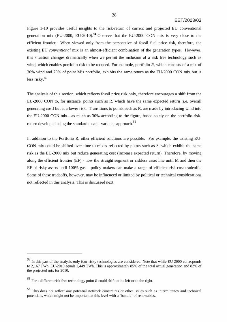
Figure 1-10 provides useful insights to the risk-return of current and projected EU conventional

generation mix (EU-2000, EU-2010).54 Observe that the EU-2000 CON mix is very close to the

efficient frontier. When viewed only from the perspective of fossil fuel price risk, therefore, the

existing EU conventional mix is an almost-efficient combination of the generation types. However,

this situation changes dramatically when we permit the inclusion of a risk free technology such as

wind, which enables portfolio risk to be reduced. For example, portfolio R, which consists of a mix of

30% wind and 70% of point M’s portfolio, exhibits the same return as the EU-2000 CON mix but is

less risky.55

The analysis of this section, which reflects fossil price risk only, therefore encourages a shift from the

EU-2000 CON to, for instance, points such as R, which have the same expected return (i.e. overall

generating cost) but at a lower risk. Transitions to points such as R, are made by introducing wind into

the EU-2000 CON mix—as much as 30% according to the figure, based solely on the portfolio risk-

return developed using the standard mean - variance approach.56

In addition to the Portfolio R, other efficient solutions are possible. For example, the existing EU-

CON mix could be shifted over time to mixes reflected by points such as S, which exhibit the same

risk as the EU-2000 mix but reduce generating cost (increase expected return). Therefore, by moving

along the efficient frontier (EF) - now the straight segment or riskless asset line until M and then the

EF of risky assets until 100% gas – policy makers can make a range of efficient risk-cost tradeoffs.

Some of these tradeoffs, however, may be influenced or limited by political or technical considerations

not reflected in this analysis. This is discussed next.

54

In this part of the analysis only four risky technologies are considered. Note that while EU-2000 correspondsto 2,167 TWh, EU-2010 equals 2,449 TWh. This is approximately 85% of the total actual generation and 82% ofthe projected mix for 2010.

55 For a different risk free technology point R could shift to the left or to the right.

56 This does not reflect any potential network constraints or other issues such as intermittency and technical

potentials, which might not be important at this level with a ‘bundle’ of renewables.

29EET/2003/03

Portfolio R isk and Returnfuel risk

0.25

0.27

0.29

0.31

0.33

0.35

0.37

0.00 0.05 0.10 0.15 0.20 0.25 0.30

RISK: Portfolio Standard Deviation

Por

tfo

lio R

etu

rn [

kWh

/cen

t]

E fficient F rontierwith no inclus ion ofwind

100% coal

100% oil

100% gas

100% nuclear

EU 2000 Conventional20.3% gas32.0% coal 7.8% oil 39.9% nuclear

R :30% wind 70% M

M:41 % gas 42 % coal 0 % oil17 % nuclear

S

EU 2010 Conventional

100% wind

P

P:10.0% gas 40.2% coal 5.6% oil 44.2% nuclear

Figure 1-10 Portfolios of four conventional technologies applied to the EU – fuel risk

Optimality and practical feasibility of the 2010 portfolios

The last section illustrated the point that when fuel price is the only risk, the range of efficient or

optimal generating portfolio choices will include some proportion of riskless or fixed cost technologies

such as wind. However, practical and other constraints may alter the efficient solutions presented. For

example, the feasible solution may contain more nuclear because plants cannot or will not be

decommissioned in the near future. This section explores solutions that may be practically more

feasible than those of the last section, and evaluates the extent to which these solution affect risk and

return. Figure 1-11 shows the projected EU 2010 CON mix.57 This 2010 mix can reasonably be

assumed to correspond to the outcome of current policies projected to 2010.

Compared to the EU-2000 CON, the EU 2010 CON mix is riskier and offers higher returns (lower

costs).58 No economic gain is produced for society by moving from the EU-2000 CON to her

projected 2010 mix: the move reduces generating costs, but increases risk. This means that some

members of society will be pleased, while other, more risk-averse members will be less happy.

Overall, the move produces no efficiencies or welfare gains.

Further, as compared to M, the optimal conventional mix, the EU-2010-CON-mix contains more oil

and more nuclear, but less gas and coal. Its risk and return are both lower than M. Unlike M, the EU-

57

Prepared by Electricity Information (2001)

58 Note that they correspond to different amounts of electricity generated.

30EET/2003/03

2010 CON-mix is less than efficient in the sense that both its risk and return can be improved by

adding fixed-asset resources to the mix. For example, by introducing wind, the risk-return of the EU-

2010 CON will shift to points such as R’, which represent improvements that produce societal welfare

gains. These gains are created because the same electricity is produced at lower risk (points R’). In

short, the politically feasible solutions represented by EU-2010-CON are inferior to the ones

composed of M and a risk-free technology.

Finally, we examine a scenario consisting of a portfolio with no oil since its actual share in the EU

generation mix is already quite low and a phase out might be desirable, cf. “EU-2010 no oil” in the

figure. This mix exhibits lower risk and return than both EU-2010 CON and EU-2000 CON. The

inclusion of wind, which results in a mix of wind & “EU-2010 no oil”, would lead to significantly

lower risk / return than with EU-2010 CON.

The previous sections have discussed the efficiency of various generating portfolios and shown the

possible tradeoffs policy makers might choose along the efficient frontier. However, the previous

graphs have not explicitly shown the changing technology mix along the efficient conventional

frontier. This is given in Figure 1-12, which shows how the mix of conventional fuels changes along

the efficient frontier. The results more clearly display the technology shifts needed to move along the

frontier. For example, high risk/high return portfolios are dominated by gas generation. As risk and

returns fall, (i.e. as costs rise), the share of gas declines while the share of coal and nuclear rises. An

infinite number of portfolio mixes can be constructed to yield an overall return of 0.295 kWh/cent –

costs of 3.4 cents/kWh. However, as shown in Figure 1-10, the optimal or minimum risk

(conventional) portfolio at this return level, P, contains about 10% gas, 40% coal, 6% oil and 44%

nuclear.

Stated differently, 1-11 depicts the shape of the efficient frontier– i.e. the cost of trading off return

against risk, while Figure 1-12 shows the conventional technology changes required to make these

risk/return trade-offs.

31EET/2003/03

P ortfolio R is k and R eturnfuel r is k

0.25

0.27

0.29

0.31

0.33

0.35

0.37

0.00 0.02 0.04 0.06 0.08 0.10 0.12 0.14 0.16 0.18 0.20

RISK: Portfolio Standard Deviation

Po

rtfo

lio R

etu

rn [

kWh

/cen

t]E fficient F rontier withno inclus ion of wind

Wind & polit. feas ible

100% coal

100% gas

100% nuclear

E U 2000 Conventional20.3% gas32.0% coal 7.8% oil 39.9% nuclear

R :30% wind 70% M

M:41% gas 42% coal 0% oil17% nuclear

S

E U 2010 no oil22.0% gas 34.7% coal 0.0% oil43.3% nuclear

E U 2010 Conventional35.0% gas 24.0% coal 6.3% oil34.7% nuclear

100% wind

P

R ’:15.2% wind 84.8% M

Figure 1-11 Practically feasible solutions

Portfolio Mix Along Conventional Efficient Frontier

0%

10%

20%

30%

40%

50%

60%

70%

80%

90%

100%

0.29

50.

300

0.30

50.

310

0.31

50.

320

0.32

50.

330

0.33

50.

340

0.34

50.

350

0.35

50.

360

Returns [kWh/cent]

Sh

are

of

each

tec

hn

olo

gy

0.05

79

0.05

82

0.05

96

0.06

21

0.06

56

0.06

99

0.07

49

0.08

05

0.08

66

0.09

31

0.10

01

0.10

80

0.11

69

0.12

66

Portfolio fuel risk

nuclear

oil

coal

gasGAS

NUCLEAR

COAL

P

Figure 1-12 Portfolio mix along the efficient conventional frontier - fuel risk

32EET/2003/03

This section has introduced the portfolio concepts and shown how the analysis can provide important

guidance to policy makers. The next section explores the portfolio analysis using a more realistic case

that reflects the variability of O&M costs.

Adding operation and maintenance cost risk

The previous section introduced the portfolio analysis methods using models that reflected only fuel

price risk. Though simplified, these models are most likely unbiased to the extent that fossil price

risks dominate other portfolio risks. The simplified models produce useful insights regarding the

optimality of existing and projected generating portfolios for the European Union. The primary

conclusions of the simplified model is that the addition of wind and other fixed-cost technologies to

the EU-2000-conventional mix and the EU-2010-CON-mix serves to produce welfare or efficiency

gains in the form of risk and cost reduction.

This section extends the analysis, by adding the risks associated with O&M outlays. The addition of

O&M risk captures all market risk associated with existing plants since their investment costs are

already sunk and hence represent no risk.59 The addition of construction period risks for new capacity,

discussed in later sections, involves discriminating between new and existing generation capacity,

which also enables us to distinguish between the costs and efficiencies of each. The final set of optimal

portfolios presented in Section 3.4 therefore reflects efficiency gains and cost reduction for new

capacity additions as well as the additional construction period risks they will encounter. We note

however, that the general message of the simplified fuel-risk-only model discussed in the previous

section does not materially change as its complexity and sophistication is increased.

Capital intensive, renewable technologies, such as wind, PV, hydro, geothermal, solar thermal, etc. are

risk free when only fuel risk is considered as discussed in the last section. When O&M risk is added,

these technologies in fact bear some degree of market or cost risk. The O&M costs of renewable

technologies, will vary in systematic manner and will also exhibit some degree of systematic

covariance with the O&M costs of other technologies. This eliminates the straight-line portion of the

efficient frontier shown in the last section.

A proxy method for estimating O&M risk

In the case of financial assets, estimates of historic variability are performed using historic HPR data.

In the case of O&M costs, given sufficient historic cost data, the variances and co-variances could

likewise be estimated in the usual manner. However, we did not have access to such data and

therefore estimated O&M cost risk using financial proxies. In other words, we assumed that fixed and

59

Salvage and decommissioning costs are not considered and will be included in subsequent studies (see AnnexA).

33EET/2003/03

variable O&M costs have a risk pattern similar to the known variability of certain financial

instruments. For example, we assumed that fixed O&M costs present a "debt equivalent" risk [e.g. see

Brealey and Myers (1991) p. 473-474]. Fixed O&M costs are contractual in nature— as long as the

owner of a generating station has sufficient income, the fixed O&M will be performed. This is a risk

that is very similar to the risk of the firm's interest payments, which also will continue as long as there

is sufficient income.60 As a proxy for fixed O&M risk we therefore use estimates of the historic

standard deviation for various corporate bonds as provided by Ibbotson Associates (1998) and as

shown in Table 1-3.

We use a similar financial proxy method for estimating the historic risk or variance of variable O&M

costs. In accounting terms, variable O&M costs are, by definition, conceptualised as volume-driven,

i.e. they vary with kWh output. In addition to fluctuating with electricity output, which no doubt is

related to economic cycles, variable O&M outlays will also fluctuate with the costs of labour and

material, which also have a systematic covariance with economic activity. We assume the variable

O&M cost risk to be equivalent to the overall market risk or variability of a broadly diversified market

portfolio such as the S&P 500 (or the Morgan Stanley MCSI Europe Index). This variability is

significantly higher than the historic SD of corporate bonds (Table 1-3).

The above estimates for fixed and variable O&M are somewhat arbitrary and ideally and should be

refined and tested using actual historic field O&M cost experience. We subsequently use a series of

sensitivity analyses to further evaluate these estimates, (see Annex B). The financial proxy data used

to estimate O&M variability is given in Table 1-3, which shows the historic standard deviation of

returns for various financial assets. The standard deviation (SD) of a broadly diversified market

portfolio is approximately 20% (percentage points) while the SD for government and corporate bonds

range from 3.2% to a high of 9.2% depending on the source and time period.

60

To be precise, interest payments are somewhat less risky than O&M outlays since available income will beused to first cover these payments.

34EET/2003/03

Table 1-3 Standard deviations of total returns for different assets61

Time Period mean62

[%]AnnualSD [%]

Type of Security Source

1926-1997 17.7 33.9 Small company stocks Ibbotson Associates (1998), p. 122 Table 6-71926-1997 13.0 20.3 Large company stocks Ibbotson Associates (1998), p. 122 Table 6-71928-2001 12.1 20.1 Stocks (S&P 500) 63 New York University, Leonard N. Stern

School of Business64

1926-1997 5.6 9.2 Long-term Governmentbonds

Ibbotson Associates (1998), p. 122 Table 6-7

1926-1997 6.1 8.7 Long term Corporate bonds Ibbotson Associates (1998), p. 122 Table 6-71926-1998 3.8 3.2 Treasury bills Ibbotson Associates (1998), p. 122 Table 6-7

Historic labour costs provide a second means for estimating the SD of O&M. Such estimates should

be reasonable to the extent that systematic fluctuations in fixed and variable O&M costs are caused by

labour cost changes. Table 1-4 shows the estimated standard deviations for a set of historic labour cost

data for various countries. The three data sources must be compared with caution since the analysed

time periods, the sectors and the statistical methods and definitions used are different for each. This

being said, the calculated standard deviations are in the range of 1.6% and 10.7%.

For the analysis presented in this report, we use the financial proxy estimates and, as previously

mentioned, coupled with sensitivity analyses, (see Annex B), which suggest our results are sufficiently

consistent. We therefore leave the estimation of more reliable O&M standard deviations to future

work. The following analysis is based on a standard deviation of 8.7% for the fixed O&M and 20%

for the variable O&M.

61

Not inflation adjusted, percentages (%) are “percentage points”

62 Arithmetic mean

63 Weighted index of 500 stocks often used as an estimation of the performance of the whole market.

64 http://www.stern.nyu.edu/%7Eadamodar/pc/datasets/histretSP.xls, last accessed 17 Jun. 02

35EET/2003/03

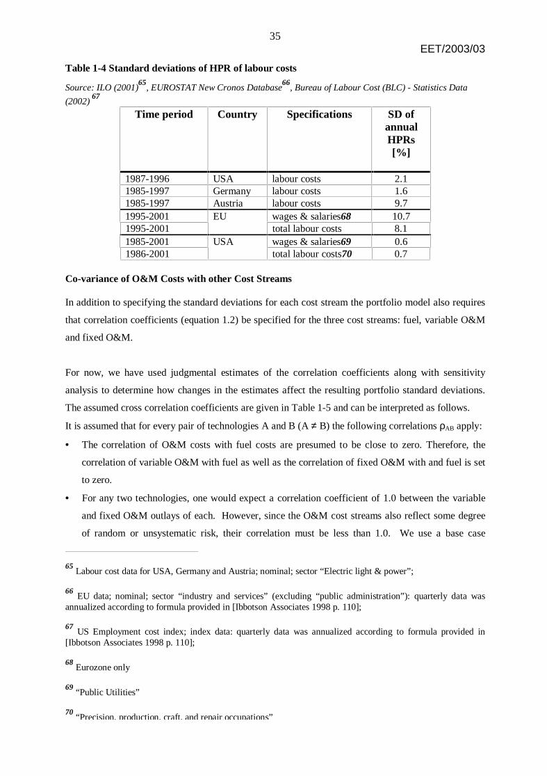
Table 1-4 Standard deviations of HPR of labour costs

Source: ILO (2001)65

, EUROSTAT New Cronos Database66

, Bureau of Labour Cost (BLC) - Statistics Data

(2002) 67

Time period Country Specifications SD ofannualHPRs[%]

1987-1996 USA labour costs 2.11985-1997 Germany labour costs 1.61985-1997 Austria labour costs 9.71995-2001 EU wages & salaries68 10.71995-2001 total labour costs 8.11985-2001 USA wages & salaries69 0.61986-2001 total labour costs70 0.7

Co-variance of O&M Costs with other Cost Streams

In addition to specifying the standard deviations for each cost stream the portfolio model also requires

that correlation coefficients (equation 1.2) be specified for the three cost streams: fuel, variable O&M

and fixed O&M.

For now, we have used judgmental estimates of the correlation coefficients along with sensitivity

analysis to determine how changes in the estimates affect the resulting portfolio standard deviations.

The assumed cross correlation coefficients are given in Table 1-5 and can be interpreted as follows.

It is assumed that for every pair of technologies A and B (A ≠ B) the following correlations ρAB apply:

• The correlation of O&M costs with fuel costs are presumed to be close to zero. Therefore, the

correlation of variable O&M with fuel as well as the correlation of fixed O&M with and fuel is set

to zero.

• For any two technologies, one would expect a correlation coefficient of 1.0 between the variable

and fixed O&M outlays of each. However, since the O&M cost streams also reflect some degree

of random or unsystematic risk, their correlation must be less than 1.0. We use a base case

65

Labour cost data for USA, Germany and Austria; nominal; sector “Electric light & power”;

66 EU data; nominal; sector “industry and services” (excluding “public administration”): quarterly data was

annualized according to formula provided in [Ibbotson Associates 1998 p. 110];

67 US Employment cost index; index data: quarterly data was annualized according to formula provided in

[Ibbotson Associates 1998 p. 110];

68 Eurozone only

69 “Public Utilities”

70 “Precision, production, craft, and repair occupations”

36EET/2003/03

estimate of 0.7. To put it differently, we assume as a base case that the correlation coefficient for

the O&M costs of any two technologies will be ρAB = 0.7.

• The correlation coefficient between variable and fixed O&M is presumed to be low, and is set to

0.1.

Table 1-5 Assumed cross-correlations for the cost streams of existing generation assets

Technology BFuel Variable

O&MFixed O&M

Fuel Table 1-271 0 0Variable O&M 0 0.7 0.1

Tec

hnol

ogy

A

Fixed O&M 0 0.1 0.7

Results using the base case proxy risk estimates

Figure 1-13 shows the portfolio results using the base case proxy risk estimates. Five risky

technologies are considered, i.e. gas, coal, oil, nuclear and wind.72 The figure gives only the

efficient frontier; other information is removed in the interest of clarity. The results indicate that when

fuel and O&M cost risk is included, the EU-2000 mix is reasonably close to the efficient frontier, as

was the case for the simplified fuel-risk only model of the previous section. In addition, even though

the efficient frontier now reflects the addition of O&M risk, the relative location of the EU-200073 and

EU-2010 mixes with respect to each other and the efficient frontier are quite similar to what they were

with the fuel-risk-only model of Section 3.2.

Further, the results indicate that, as before, it is possible to costlessly improve on the EU-2000 mix.74

This can be done by including more wind, which creates portfolios with both lower cost and risk. For

example, portfolio N, on the efficient frontier, is less risky than the EU-2000 mix but has the same

return or generating cost. N contains no oil, more wind and coal, and less nuclear and gas generation.

71

This correlation is calculated on the basis of HPRs of historical fuel prices.

72 Note that in Electricity Information (2001) wind is added up with “solar” and “tide”. However, since the

electricity generation of solar and tide is (and will be) very small compared to wind, it is basically only wind.The 5 technologies make up approximately 86% of the generation mix together [Electricity Information (2001)].Hydro is excluded from this mix.

73 Contrary to the preceding sections the EU-2000 mix now contains wind. We included it because with the

O&M risk wind becomes a risky asset like the four conventional technologies.

74 Under the conditions specified before, e.g. zero transaction costs.

37EET/2003/03

Portfolio Risk and Returnfuel and O&M risk

0.25

0.27

0.29

0.31

0.33

0.35

0.37

0.00 0.02 0.04 0.06 0.08 0.10 0.12 0.14 0.16 0.18 0.20

RISK: Portfolio Standard Deviation

Po

rtfo

lio R

etu

rn [

kWh

/cen

t]

efficient frontier

100% coal

100% oil

100% gas

100% nuclear

EU 2010 gen mix - 5 tgies34.0% gas 23.4% coal 6.1% oil33.7 % nuclear 2.8% wind

EU 2000 gen mix - 5 tgies20.1% gas 31.7% coal 7.7% oil 39.5% nuclear 1.0% wind

100% wind

O

O:16.4% gas 59.7% coal 0.0% oil 23.9% nuclear 0.0% wind

N N:14.1% gas 51.7% coal 0.0% oil 26.9% nuclear 7.2% wind

P

P: 1.4% gas 8.5% coal 1.0% oil 21.7% nuclear 67.5% wind

Figure 1-13 Portfolios of four conventional technologies – fuel and O&M risk75

Alternatively, note portfolio O with the same risk as the EU-2000 mix but with lower cost (higher

return). Portfolio O contains approximately 60% coal, 16% gas and 24% nuclear with no wind. There

are other possible portfolios between O and N, all of which are superior to the EU-2000 mix.

Similarly, the projected EU-2010 mix is also inefficient, and can be improved, by moving to e.g. point

O although this now implies a significant increase in the share of coal (from 23% to 59%) and a

decrease in gas, nuclear, and wind. Any increases in the share of wind would now be represented by a

move down the efficient frontier, e.g. moving to the 7.2% share of wind represented by portfolio N

will reduce return or increase cost by 2.5%. When O&M costs are included, the addition of more wind

to the EU-2010 mix is not costless, yet, it yields the benefit of reducing risk by about 15.9%. This

result changes when new costs estimates for capacity additions as well as construction period risks are

included subsequently.

Note that the efficient frontier ends with portfolio P, which comprises mainly wind (68%) and nuclear

(22%) and only little gas and coal - see also Figure 1-14 below.76

75

When comparing Figure 1-13 with Figure 1-10 portfolio risk in the former seems to be generally higher thanin the latter. That is due to the fact that the measurement of risk has now changed. This new scaling will howeverremain constant throughout the rest of the paper. See also footnote 45.

38EET/2003/03

Finally, Figure 1-14 shows the changes in technology shares as the portfolio mix moves up the

efficient frontier from P to 100% gas. While significant shares of wind occur at lower risk–return

mixes, coal and gas dominate the higher risk–return portfolios. The share of oil never rises above

1.1% while the percentage of nuclear reaches a maximum of 27%, (at risk / return 0.03-0.305),

significantly lower than its 40% share in the current EU-2000 mix.

Portfolio Mix Along the Efficient Frontier

0%

10%

20%

30%

40%

50%

60%

70%

80%

90%

100%

0.26

0.27

0.28

0.29

0.30

0.31

0.32

0.33

0.34

0.35

0.36

Returns [kWh/cent]

Sh

are

of

each

tec

hn

olo

gy

0.01

76

0.01

83

0.02

08

0.02

46

0.02

90

0.03

40

0.03

97

0.04

60

0.05

58

0.06

88

0.08

36

Portfolio fuel and O&M risk

windnuclearoilcoalgas

GAS

NUCLEAR

WIND

COAL

NP

Figure 1-14 Portfolio mixes along the efficient frontier – fuel and O&M risk

Completing the analysis: New and existing generation capacity

Previous sections have presented a range of efficient portfolio solution for the EU. These solutions

were based on the assumption that both new and existing capacity has the same set of costs, and that

fuel and O&M costs are the only risks. This section extends the analysis and presents a conceptually

more sophisticated model that distinguishes between existing and new capacity and hence explicitly

models the costs and attendant risks for "new" as well as existing gas, coal and wind capacity.77 The

76

Observe that such high shares of wind are of course not feasible since technical potentials according to Huberet al. 2001 limit wind to 7.9% in 2010.

77 An increased electricity demand is generally met by building new capacity. Electricity produced depends on

the dispatch of available capacity, i.e. on annual full load hours of each installed capacity. Since the presentedmodel does not deal with installed capacity but with electricity generated it implies average full load hours.

39EET/2003/03

model now consists of a 7-technology mix, four old technologies — coal, gas, oil and nuclear, and

three new ones — wind, gas and coal.

We do not include “new” nuclear capacity additions on the basis of the apparent widespread political

climate opposing this technology in Europe (with Finland as the exception). Likewise, we do not

include new oil capacity in accordance with the EU-2010 forecast [Electricity Information (2001)].

Finally, since the current share of wind in the EU-2000 mix is so low — less than 1% — we do not

differentiate between “new” and “existing” wind, but rather model all wind as new. This allows us to

simplify the analysis and presentation without sacrificing much realism.

The current model also does not include decommissioning and salvage costs, or other possible

transition costs from current to future portfolios. As a consequence, we speculate that the share of

existing technologies in the (feasible) efficient portfolios may be understated while the share new

technologies may be overstated [Figure 1-15 and Figure 1-20]. This can be partly corrected by

constraining existing capacity so it exactly equals its year-2000 generation in the EU mix [e.g. see:

Herbst (1990) p. 307]. We do this for the case of nuclear capacity, arguing that economics aside, it is

unlikely that much nuclear capacity will be decommissioned over the next 7-10 years. We compare

this "practically constrained" optimum to a more globally efficient, unconstrained set of results which

we offer in the spirit of a first-step exploration of the range of efficient solutions.78

Costs and Risks for New and Existing Capacity

Distinguishing between existing and new technology allows us to explore a range of more realistic

portfolio scenarios. For example, construction period risk affects only new generation. Also, new

capacity has different capital and operating costs, which are generally lower. However, to the extent

that some new technologies, such as many renewables, are on a steeper learning or cost curve [IEA

(2000)], applying the same costs to both new and old generating capacity, as we did in previous

sections, likely understates the share of renewables in the efficient mix.

Table 1-6 shows the levelised annual costs for the current and new vintage of generating technologies.

The costs are further categorised by cost type - e.g. levelised investment cost, fuel, and fixed and

variable O&M.

78

We also apply a set of technical or feasibility constraints that insure that no additional existing (year-2000)capacity is added to the 2010 mix

40EET/2003/03

Table 1-6 Levelised annual costs of technologies for new and existing generation capacity

GAS COAL OIL79 NUCLEAR WINDLEVELIZED

COSTUS cents / kWh Existing

CCGTNew

CCGTSteamboiler

Newsteamboiler

Existing New

Fixed investment 0.64 0.59 1.24 1.18 0.59 2.26 3.08 2.80Fuel 1.82 1.75 1.33 1.30 2.08 1.00 0.00 0.00Variable O&M 0.13 0.13 0.28 0.28 0.15 0.03 0.00 0.00Fixed O&M 0.18 0.18 0.28 0.28 0.15 0.66 0.89 0.89Total busbar cost 2.76 2.65 3.14 3.05 2.96 3.95 3.97 3.69Return(kWh/US cents) 0.362 0.378 0.318 0.328 0.337 0.253 0.252 0.271

The levelised costs in table 1.6 are derived from the IEA World Energy Outlook 2000 (WEO 2000).

WEO 2000 is a widely circulated and highly regarded source of current and future energy

information.80 However, in the case of financial portfolios, theory holds that current share prices

represent a risk-adjusted present value of all future cash flows. For the time being, we chose to use a

traditionally determined and widely accepted set of generating costs such as those produced by the

WEO 2000. However, in a subsequent sensitivity analysis (Annex B) we use a set of risk-adjusted

generating costs, which generally show that relative to fossil technologies, renewables are

considerably more cost effective. The risk-adjusted costs therefore produce efficient portfolios with

lower fossil fuel shares.

Planning and construction period risks and cross-correlation

Lumpy technology additions produce numerous construction period risks. Longer planning and

construction periods especially increase the likelihood that economic and technological changes will

affect cost. In this section we again use the proxy risk measure approach to establish a reasonable set

of base-case estimates for construction period risk. Future analyses would undoubtedly benefit from

actual project reviews, where they are available, in order to develop potentially better estimates of

these risks.

The analysis presented in this and subsequent sections is based on the assumption that construction

period costs will fluctuate in a manner similar to the historic fluctuations of a broadly diversified

market portfolio (whose beta = 1.0). Based on this assumption, we estimated construction period risk

79

These calculations are by the authors.

80 Future costs are computed on the basis of WEO (2000) by means of interpolation.

41EET/2003/03

to be approximately 20% (Table 1-3 page 34). This base case variability is applied to the construction

period risk of all lumpy additions: coal, gas, oil and nuclear, although different estimates are used later

in the sensitivity analysis. By contrast, wind, PV, and other modular technologies will by definition

exhibit little construction period risk [e.g. Hoff (1997), Brower et al. (1997) and Venetsanos et al.

(2002)]. For these modular technologies the SD for construction period risk is therefore set to zero.

Finally, estimating portfolio risk requires us to estimate the cross-correlation coefficients between the

construction period costs for a given technology and other costs. These estimates are made using the

approach already described earlier, (Table 1-5 p. 36). For every pair of technologies A and B (A ≠ B) a

cross correlation coefficient, ρAB, is assumed for the linkage between investment and O&M costs

(Table 1-7). These are supposed to be quite small — 0.1. Next, as discussed in preceding sections, the

correlation coefficient of investment costs for two different technologies is set to 0.7 (Table 1-7).

Finally, the empirically derived cross-correlations estimates for the HPRs of fuel prices are given in

Table 1-8.

Table 1-7 Assumed cost cross-correlation when construction period risks areincluded

Technology B

Category ConstructionPeriod

Fuel VariableO&M

FixedO&M

ConstructionPeriod

0.7 0 0.1 0.1

Fuel 0 Table 1-881 0 0Variable O&M 0.1 0 0.7 0.1

Tec

hnol

ogy

A

Fixed O&M 0.1 0 0.1 0.7

81

This correlation coefficient is calculated on the basis of HPRs of historical fuel prices.

42EET/2003/03

Table 1-8 Empirically derived fuel cross-correlations estimates for existing and new vintagetechnologies82

GAS STEAMCOAL

CRUDE OIL ENRICHEDURANIUM

NEW GAS NEWCOAL

GAS - 0.48 0.46 -0.27 - 0.48STEAM COAL 0.48 - 0.24 -0.13 0.48 -CRUDE OIL 0.46 0.24 - -0.37 0.46 0.24URANIUM -0.27 -0.13 -0.37 - -0.27 -0.13NEW GAS - 0.48 0.46 -0.27 - 0.48NEW COAL 0.48 - 0.24 -0.13 0.48 -

As discussed previously, the total risk or standard deviation associated with new capacity additions is

higher relative to existing assets because for the latter group, construction period risks are sunk and

hence riskless. On the other hand, new capacity additions often involve newer vintage technologies,

which inevitably exhibit technologically driven efficiency gains and cost reductions. These appear as

higher expected returns in our construct.

Base-Case Results

Figure 1-15 shows the base case results. Even though the model is now a much better representation of

reality, the basic picture seems to be remarkably similar to the results yielded by the relatively simpler

models of earlier sections. This is due to the dominance of fuel price risk on the calculations. Observe

that the positioning of the EU-2000 and EU-2010 mixes relative to the efficient frontier and each other

is almost unchanged.83

82

Since wind does not exhibit any fuel costs its correlation coefficient with the other technologies is zero andtherefore not included.

83 Note that EU-2000 and EU-2010 are based on different generation levels. While the former corresponds to ca.

2190 TWh, the latter equals 2520 TWh. All mixes shown in the portfolio graph of this section, but the EU-2000mix, refer to the generation level of EU-2010.

43EET/2003/03

Portfoliorisk and Return

0.25

0.27

0.29

0.31

0.33

0.35

0.37

0.39

0.00 0.02 0.04 0.06 0.08 0.10 0.12 0.14 0.16 0.18 0.20

RISK: Portfolio Standard Deviation

Po

rtfo

lio R

etu

rn [

kWh/

cen

t]

efficient frontier

100% old coal

100% oil

100% old gas

100% old nuclear

E U 2010 gen mix - 5 tgies16.6% old gas 26.1% old coal 6.4% oil32.6% nuclear 2.7% wind15.7% new gas

EU 2000 gen mix - 5 tgies20.1% gas 31.7% coal 7.7% oil 39.5% nuclear 1.0% wind

100% wind

N N: 7.6% old gas 41.6% old coal 46.3% wind 4.5% new gas

P

P: 2.3% old gas 12.2% old coal 1.0% oil24.8% nuclear 59.7% wind

Q:15.3% old gas 33.3% old coal51.4% new gas

100% newgas

100% new coal

U

Figure 1-15 Base case efficient portfolios: fuel, O&M and construction period risks for existingand new capacity

As was the case in previous sections, Figure 1-15 suggests that it is possible to costlessly improve the

EU-2000 mix by constructing future portfolios such as N, with the same costs but lower risk. N, which

is superior to the EU-2000 mix and hence increases societal welfare, contains approximately 8% old

gas, 42% old coal, 5% new gas and 46% wind.84 Alternatively, policy makers could choose portfolios

with lower risk by moving down the efficient frontier to points such as P, which comprises 60% wind,

25% old nuclear, some old coal and very small shares of old gas and oil. Similarly the EU-2010 mix

can also be improved by moves to the efficient frontier.85 Although not depicted here, such portfolios

would contain added amounts of wind as discussed in subsequent sections.

Finally, Figure 1-16 depicts the technology shares at different risk/return levels, which help policy

makers understand the required technology trade-offs for moves along the efficient frontier of Figure

1-15. Interestingly and somewhat surprisingly, the efficient frontier contains no “new coal”. This

84

Note that such high shares of wind are of course not feasible since technical potentials according to Huber etal. 2001 limit wind to 7.9% in 2010.

85 Observe that while EU-2010 includes new and old gas, coal, oil, nuclear and wind, from a mean-variance

perspective it lies very close to, and hence could be replaced entirely by a single technology— old coal.

44EET/2003/03

comes from the fact that “new coal” exhibits the highest investment period risk because its share of

investment costs (see Table 1-6) is the highest among the new non-modular technologies.

At lower risk/return levels, wind and old coal dominate the mix, while for high risk–low cost (high

return) portfolios, the efficient mixes consist primarily of new and old gas and some old coal. At return

levels above 0.30 kWh/cent nuclear is no longer contained in the mix (see line in Figure 1-16).

Portfolio Mix Along the Efficient Frontier

0%

10%

20%

30%

40%

50%

60%

70%

80%

90%

100%

0.28

0.29

0.30

0.31

0.32

0.33

0.34

0.35

0.36

0.37

Return [kWh/cent]

SH

AR

E o

f ea

ch te

chn

olo

gy

0.019

0.022

0.026

0.032

0.038

0.045

0.054

0.064

0.077

0.090

PORTFOLIO RISK

WIND

OLD COAL

OLD GAS

NEW GAS

OL D NUCL E AR

Figure 1-16 Portfolio mix along the efficient frontier: fuel, O&M and construction period risksfor new and old capacity

Technical Feasibility of the 2010 Portfolios

Compared to the EU-2000 generation mix, the projected EU-2010 mix exhibits a higher risk coupled

with higher return (Figure 1-15). While some may prefer this risk-return combination, it cannot be

said to be economically superior to the EU-2000 mix. This can be understood by illustration: some

people prefer to invest in riskier stocks while others like bonds, but neither of these is "superior" or

more efficient. In fact, the increased return (cost reduction) of the EU-2010 almost exactly equals its

percentage risk reduction.

Moreover, the projected EU-2010 mix is inefficient. It does not lie on the efficient frontier, though it

comes close, indicating that better portfolios such as U (Figure 1-16) exist. These would likely include

higher shares of old coal (71.9%) along with a higher share of wind. However, a share of almost 80%

of “old coal” in an EU 2010 mix is of course not feasible.

45EET/2003/03

Feasible solutions can be obtained by constraining the shares of existing technologies in the efficient

frontier so that they cannot exceed their actual EU-2000 generation. Therefore, for example “old coal”

does not exceed a share of 27.5% in the mixes for 2010. This produces efficient solutions (Figure 1-

17) that are technically feasible. Such solutions lie along what we term the feasible efficient frontier

(FEF). Observe that the FEF lies just slightly to the right of the efficient frontier. Points U on the

efficient frontier and Point V on the FEF produce the same expected return but V, on the FEF, exhibits

7.3% more market risk. Compared to Portfolio U, V contains more wind (25% vs. 3%), old gas (18%

vs. 10%) and new gas (26% vs. 15%) as well as some new coal (4%).

Portfolio R isk and Returnfuel and O&M risk vs new investment

0.25

0.27

0.29

0.31

0.33

0.35

0.37

0.39

0.00 0.02 0.04 0.06 0.08 0.10 0.12 0.14 0.16 0.18 0.20

RISK: Portfolio Standard Deviation

Po

rtfo

lio R

etu

rn [

kWh

/cen

t]

feas ible efficient frontier

efficient frontier

100% old coal100% oil

100% old gas

100% old nuclear

EU 2010 gen mix - 5 tgies17.5% old gas 23.4% old coal 6.1% old oil33.7% old nuclear 2.8% wind16.5% new gas

E U 2000 gen mix - 5 tgies100% wind

P

P: 2.3% old gas 12.2% old coal 1.0% old oil24.8% nuclear 59.7% wind

100% newgas

100% new coal

U:10.0% old gas 71.9% old coal 3.3% wind14.8% new gas

V:17.5% old gas 27.5% old coal 24.7% wind25.9% new gas 4.4% new coal

Figure 1-17 Efficient feasible portfolios: fuel, O&M and construction period risk for existing andnew capacity

Figure 1-18 shows the portfolio mix along the FEF. Since “old coal” is limited to its actual EU-2000

generation – corresponding to 27.5% in the 2010 mixes - other technologies replace “old coal” at

return levels where this limit is exceeded. At point U (0.33 kWh/cent) coal attains its maximum share

(71.9%) of the efficient frontier (see Figure 1-17). In the FEF the exceeding 44.4% “old coal” (71.9%

minus 27.5%) are replaced primarily by wind, some gas, “new coal” and “new gas”. Note that “new

coal” is a new entrant to the FEF and attains a maximum share of 6%.

46EET/2003/03

Portfolio Mix Along the Feasible Efficient Frontier

0%

10%

20%

30%

40%

50%

60%

70%

80%

90%

100%

0.28

0.29 0.30

0.31

0.32

0.33

0.34

0.35

0.36 0.37

Return [kWh/cent]

Sha

re o

f ea

ch t

ech

nolo

gy

0.019

0.022

0.027

0.033

0.041

0.049

0.058

0.067

0.077

0.090

Portfolio risk

new coal

new gas

wind

old nuclear

old oil

old coal

old gas

WIND

COAL

OLD GAS

NEW GAS

NUC

O

Figure 1-18 Portfolio mix along the feasible efficient frontier – fuel, O&M construction periodrisk

The Effect of practical constraints on the efficient solutions

The feasible efficient portfolios presented in the last section contain 0% nuclear at returns in excess of

0.30 kWh/US cent, see mix O in Figure 1-18. A 0% nuclear share is obviously not a politically or

practically feasible solution for any 2010 portfolio, since it is inconceivable that the vast European

nuclear capacity could be dismantled in the next seven years. This solution occurs because, as

discussed above, the current formulation of the model contains no decommissioning costs and hence

abandoning existing nuclear is costless — which does not hold in reality. Eliminating nuclear from the

EU-2010 portfolio would require major decommissioning outlays, which are also a priori risky.

Future versions of the portfolio model will include nuclear decommissioning and retirement costs for

other technologies. This will produce solutions that are more "practically feasible".

However, practical efficient portfolios can be approximated by constraining nuclear generation to its

actual generation level86 so that it maintains its 34.3% share of the EU-2010 mix. This produces

solutions that are more reasonable with respect to nuclear capacity. These solutions lie along what we

call the practical efficient frontier (PEF).

86 This is in addition to the constraints introduced for the feasible efficient frontier in the last section.

47EET/2003/03

Constraining nuclear has important effects so that the PEF differs significantly from the FEF as

illustrated in Figure 1-19. The PEF clearly moves to the right, so that it just about passes through the

projected EU-2010 mix, as might be expected. Point V on the FEF produce the same return as W, on

the PEF, but W exhibits 18% more market risk. This might be one measure of the economic cost

associated with the practical constraints. Compared to portfolio V, W contains significantly less old

coal (4.1% vs. 27.5%), more nuclear (34.3% vs. 0%), more new gas (45.5% vs. 25.9%) and no wind.

Second, constraining nuclear as we did severely reduces the maximum portfolio return levels

compared to the technically feasible solution (Figure 1-19). While the maximum portfolio return of the

FEF is the same as the return for new gas, i.e. 0.378 kWh/cent, the maximum return of the PEF is only

0.335 kWh/cent (point E in Figure 1-19). This might be another measure of the cost of the practical

constraint. Observe that point E consists of 34.3% nuclear and 65.7% new gas.87

Portfolio R isk and Return

0.25

0.27

0.29

0.31

0.33

0.35

0.37

0.39

0.00 0.02 0.04 0.06 0.08 0.10 0.12 0.14 0.16 0.18 0.20

RISK: Portfolio Standard Deviation

PO

RT

FO

LIO

RE

TU

RN

[kW

h/c

ent]

technically feas ible efficientfrontierpolitically efficient frontier

100% old coal

100% oil

100% old gas

100% old nuclear

E U 2000 gen mix - 5 tgies

100% wind

P

P: 2.5% old gas 10.5% old coal 1.5% old oil34.3% old nuclear 51.2% wind

100% newgas

100% new coal

W:16.1% old gas 4.1% old coal 34.3% old nuclear45.5% new gas

E

V:17.5% old gas 27.5% old coal 24.7% wind25.9% new gas 4.4% new coal

EU 2010 gen mix - 5 tgies17.5% old gas 23.4% old coal 6.1% old oil33.7% old nuclear 2.8% wind16.5% new gas

E :34.3% old nuclear 65.7% new gas

Figure 1-19 Efficient practically feasible portfolios: fuel, O&M and construction period risk forexisting and new capacity

87

We are of course aware of the fact that only approximately 10% of the generating capacity will realisticallychange till 2010. Therefore, extreme solutions, such as a mix of 34% old nuclear and 67% new gas, are notpractically feasible. However, we did not exclude these solutions from the politically efficient mixes a priori.

48EET/2003/03

Figure 1-20 shows the portfolio mix along the PEF. Since nuclear is constrained to its actual

generation its share rests constant over the whole PEF. This is mainly at the expense of wind but also

of old coal at higher return levels.

The actual EU-2000 mix can, as before, be improved by introducing wind into the mix. At the same

return level as the EU-2000 mix, i.e. 0.302 kWh/cent (mix N), the efficient solution would contain

17.1% old gas, 27.5% old coal, 34.3% nuclear, 12.2% wind, 7.7% new gas and 1.2% new coal.

Portfolio Mix Along the Politically Efficient Frontier

0%

10%

20%

30%

40%

50%

60%

70%

80%

90%

100%

0.27

0.28 0.29

0.30

0.31

0.32 0.33

Return [kWh/cent]

Sha

re o

f ea

ch t

echn

olo

gy

0.019

0.019

0.023

0.029

0.036

0.046

0.058

Portfolio risk

new coal

new gas

wind

nuclear

oil

old coal

old gas

WIND

OLD COAL

OLD GAS

NEW GAS

NUCLEAR

N

Figure 1-20 Portfolio mix along the practically efficient frontier – fuel, O&M and constructionperiod risk

Explicitly differentiating between existing and new capacity presents results that comport more closely

to real-world issues currently confronting EU policy makers. These issues include the type and share

of various technologies and the potential replacement, curtailment or abandonment of certain

technologies.

While the analysis deals with these issues explicitly, it ignores the risks and costs of salvage and

decommissioning, which may be particularly significant in the case of nuclear power plants. While the

results presented seem useful and realistic, additional analysis that reflects decommissioning and other

costs and risks may further improve the practically feasible results presented here. However, while

decommissioning costs are not explicitly included, we have approximated the equivalent practically

feasible solution by constraining the nuclear share to its year-2000 generation level. This has

significant effects on the portfolio and severely reduces its return levels compared to the technically

49EET/2003/03

feasible solution. It yields a set of practical solutions that illustrate the economic costs of political

policies.

Summary of important results

Our results clearly suggest that energy policy makers in Europe and elsewhere need to consider the

implications of mean-variance portfolio analysis as an input to various energy policy making and

planning processes. These policy makers are currently confronting a number of important energy

policy issues:

i. Energy Security: While energy security is widely taken as synonymous with avoiding large-

scale fuel disruptions, we have characterised a more subtle, and, we believe, highly significant

aspect of this issue: minimizing costly fossil-driven electricity price fluctuations. The prospect of

wide-scale fuel supply disruptions is certainly costly and unappealing. Yet day-to-day fuel price

increases and volatility is quite costly as well, creating economic losses that can easily run into the

tens and hundreds of billions.88

ii. Energy diversity: Like energy security, energy diversity objectives are generally not defined

explicitly, although the commonly accepted objective seems to involve creating robust energy

mixes –– i.e. efficient portfolios –– that will minimize price risk under a variety of possible

outcomes.

iii. Affordable and Reliable Electricity Costs: Creating an affordable electricity supply involves

creating portfolios with known expected price and risk characteristics. These portfolios must

reliably supply electricity in the sense of offering reasonable (affordable) long-term price streams

with reasonable volatility.

Mean-variance portfolio optimization addresses precisely these types of issues. For example, insuring

energy security (Item i) may involve a number of factors, including the diversification of supply away

from sources that may be politically unreliable. However, it is equally important to insure that the

European generating portfolio is efficient in the sense that it minimizes price risk (volatility) exposure

at any given cost level. Portfolio theory represents the only quantitative means for evaluating portfolio

efficiency, which also insures that energy diversity (Item ii) and affordability/reliability (Item iii)

objectives are implemented.

88

A summary of the literature is given in Sauter and Awerbuch (2002). The recent literature seems to suggestthat fossil price volatility itself, especially to the extent that it creates price "surprises", is as important as energyprice increases in reducing economic GDP growth.

50EET/2003/03

In general, our results indicate that the current and projected EU generating mixes are inefficient or

sub-optimal from a risk-return perspective. The analysis further indicates that portfolios with lower

cost and risk can be developed by adjusting the conventional mix and by including larger amounts of

wind or similar fixed-cost technologies. More specifically, the results suggest that increasing the share

of wind and similar fixed cost renewables in the generating mix up to levels of 12% does not increase

overall portfolio generating costs as compared to the year-2000 EU mix. Under some circumstances,

additional portfolio shares of renewables even serve to reduce overall cost and risk. This result, which

holds under a wide variety of assumed conditions, runs contrary to most analyses and to widely held

conception that given their higher stand-alone costs, adding renewables to the conventional mix can

only serve to increase overall generating cost.

While specific risk (as measured by the standard deviation of HPRs) and cost results vary as the input

assumptions, included risks and other conditions, are changed, the overall portfolio picture is

remarkably robust so that the basic message –– that the addition of fixed-cost renewables generally

reduces overall cost and risk –– changes little.

Finally, the effect of practical constraints on the optimal solution are modelled. This is done by

constraining certain technologies, in this case nuclear, to their Year-2000 generation under the

assumption that nuclear capacity will not be decommissioned over the next 7-10 years. This produces

a practically efficient frontier (PEF) and a set of practical-efficient solutions. While these are

generally inferior to the technically feasible solutions produced previously, they can still be improved

with the addition of fixed cost technologies such as renewables.

Conclusions

This analysis applies mean-variance portfolio optimization techniques to evaluate the efficiency of

current and projected EU generating mixes and to develop alternative portfolios with lower cost and

risk. The results generally indicate that the existing and projected EU generating mixes are sub

optimal - though slightly - from a risk-return perspective, which implies that feasible portfolios with

lower cost and risk exist. These can be developed by adjusting the conventional mix and by including

larger shares of wind or similar renewable technologies.

The results of the portfolio analysis suggest that fixed cost technologies such as renewables must be a

part of any efficient generating portfolio. Our assessment of all technologies is limited to risk and cost

measures, although other benefits, including low externality costs and sustainability, are often cited for

renewables.

51EET/2003/03

The analysis began with a relatively simple portfolio model. Though it included all operating and

capital costs, this model reflected only a single risk –– fuel cost risk. This risk is empirically estimated

on the basis of the historic holding period return (HPR) for fossil and enriched nuclear fuel. A striking

characteristic of the fuel risk-only-model is that the efficient frontier includes a straight-line segment

representing various mixes of wind and the conventional portfolio. This line segment exists because

wind has no fuel costs so that the standard deviation and the correlation coefficients for fuel are

reduced to zero, which produces a straight line.89, 90 On the risk axis, this line segment lies to the left

of the feasible set of conventional mixes, indicating that the inclusion of wind serves to reduce cost

and risk.

Implications for the EU Portfolio

Models that reflect the risk of fuel as well as the risk associated with fixed and variable O&M are then

introduced. This allows a more realistic evaluation of the current EU year-2000 portfolio. Specifying

O&M risk requires that the cross-correlation coefficients between wind and the conventional

technologies are specified. Since wind exhibits O&M risk, the O&M standard deviations and cross

correlations are now non-zero, so that the straight-line segment of the efficient frontier becomes a

curved segment along which lie all the possible efficient mixes.

The additional O&M risk that is now included serves to increase the overall risk. However, this

increase affects wind as well as the conventional technologies so that the principal message remains

largely unchanged: adding wind to the year-2000 and the projected year 2010 mixes might serve to

reduce cost and risk.

The standard deviations for the fixed and variable O&M costs are then estimated using financial

proxies, although future work may well benefit from an empirical analysis of the volatility of actual

historic O&M costs for different generating technologies. Financial proxies are used because

appropriate historic O&M cost data are not available. Under the approach fixed O&M costs are "debt-

equivalents" while the risk of variable O&M costs is similar to the risk of the market as a whole. Such

procedures are often used to estimate risk and discount rates in financial analyses.

89

Recall that Equation 1.2, which is the expression for portfolio risk, reduces to a straight line when one of the

variances (e.g. 2

1σ ) is set to zero. Portfolio return is also a linear function of the portfolio shares and theirreturns.

90 The choice of renewable technology affects the straight-line segment. For example, if the renewables

technology were to consist of only PV, which has virtually no operating costs, the lower end of the efficientfrontier, reflecting 100% PV, will lie much closer to the vertical axis where SD = 0.0.

52EET/2003/03

In the case of the existing year-2000 portfolio, construction period risks are not relevant. Projected

capacity additions however, will exhibit construction period risks as well as operating risks. In order

to more fully evaluate the projected 2010 EU generating mix, a more complex model that includes

planning and construction period risks is added to the fuel and O&M risks included in the previous

analyses. This enhanced model distinguishes between existing capacity and capacity additions, e.g.:

"existing" versus "new" gas and coal.

Total risk in the case of existing capacity consists of the fuel and O&M risks; in the case of new coal

and gas planning and construction period risk is also included. Wind and similar modular technologies

are characterised by short construction periods with short planning lead times, which minimizes or

essentially eliminates uncertainty during this period. In the case of wind, therefore, risks are the same

for existing and new vintages. Finally, although construction period costs are sunk, they are part of the

total cost estimate for both new and existing technologies since they are recovered through annual

charges.

By distinguishing between the projected costs of new technology vintages as compared to existing

vintages, the enhanced model also allows us to incorporate technological progress. Capital and O&M

costs for capacity additions are typically lower than the capital and O&M costs of existing vintages.

The enhanced model provides a more realistic representation of the existing and projected EU

generating mix. It uses new, lower projected costs for the capacity additions as compared to existing

capacity vintages.

The enhanced model can examine the effect of practical constraints on the optimal solutions by

developing what we term practically efficient solutions. For example, independent of underlying

economics of the mix, it seems highly unlikely that any nuclear capacity will be decommissioned

between now and the end of the decade. This constraint is included to produce a set of practical -

efficient solutions by limiting future nuclear generation to its generation in the EU-2000 mix. This

permits comparison of the practical - efficient solutions to the unconstrained or technically efficient

solutions. Constraining the nuclear generation as described has striking effects on the portfolio and

severely reduces its return levels compared to the technically feasible solution.

Though it reflects a much broader range of risks and other factors, the enhanced model continues to

support the basic message of the simple fuel-only model: i.e.: the year 2010 projected EU mix is less

than efficient. The mix can be made more efficient by adjusting the conventional technologies, and,

depending on the risk-return preferences, by adding renewables. Stated differently, it is possible to

improve the projected 2010 mix without adding more renewables, however, increasing the renewables

53EET/2003/03

share in many instances costs no more and reduces risk.91 Since environmental and other externality

benefits of renewables are not considered, this result can be seen as an additional benefit of adding

renewables to the generation mix.

As a corollary, it can be observed that current national policies that focus on gas expansion to the

exclusion of fixed cost technologies are inappropriate. In some instances, such policies will only serve

to increase risk disproportionately to any attained cost reductions. Gas expansion should not be

implemented in an economically efficient manner without a simultaneous national focus on expanding

the share of “riskless” technologies like renewables to counter the increased risk of gas.

The basic finding of this analysis therefore seems quite robust, and does not materially change even

when the risk parameter estimates are changed significantly in the sensitivity analysis. More precisely,

the sensitivity analysis alters the overall risk of the resulting portfolio, but does not change the relative

location of each alternative on the graph, nor does it materially change the shape of the efficient

frontier.

91

Note that no transition costs are considered in the present model.

54EET/2003/03

Annexes

Annex A: Assumptions and Limitations Affecting the Application of Mean-Variance Techniques

to Generating Portfolios

This paper explores the application of mean-variance Markowitz portfolio theory, originally developed

for financial assets, to the creation of optimal portfolios of generating asset. This application rests on a

set of explicit and implicit assumptions and limitations that are discussed below:

1. Indivisibility of assets: “The mean-variance portfolio model is based on the assumption that

securities are infinitely divisible, while capital investments often come in very large, indivisible

units [Seitz (1990) p. 233].”92

Our model therefore implicitly relies on the assumption that for the analysis of large service

territories or national generating portfolios, the lumpiness of capacity additions becomes relatively

less significant since total capacity needs are larger.

2. Normal distribution of holding period returns: “By looking only at mean and variance, we are

necessarily assuming that no other statistics are necessary to describe the distribution of end-of-

period wealth. Unless investors have a special type of utility function (quadratic utility function), it

is necessary to assume that returns have a normal distribution, [Copeland and Weston (1988)

p. 153].” For our analysis, it remains to be determined whether the fuel price HPRs are actually

normally distributed. However, fossil fuel prices are commonly modeled as random walks,93 [see

e.g. Felder (1994), Hassett and Metcalf (1993), Holt (1988), Glynn and Manne (1988)], which

implies that price changes are at least independent.

3. Perfectly fungible assets: Portfolio assets must be perfectly fungible: their value at any point in

time must depend only on the amount, timing and certainty of expected cash flows.

This may not always hold for generating assets where issues such as location and fuel availability

may affect selection for various reasons. Location may therefore affect asset value to the extent

that existence of, for example, a nearby gas line, may enhance the “amount, timing and certainty”

of cash flows only if a gas plant, (as opposed to a coal plant) is constructed. Technology choice

may further affect asset value to the extent that electric grid connection, siting and similar costs

may differ for different technologies.

92

See also Herbst (1990) p. 303.

93 Random walks require all the parameters of a distribution to be the same with or without an information

structure. “Furthermore, successive drawing over time must (1) be independent and (2) be taken from the samedistribution.” - [Copeland and Weston (1988) p. 348]. To put it differently, yesterday’s prices cannot be used asa basis for predicting future prices.

55EET/2003/03

4. Taxes and subsidies: Our analysis is primarily intended for public policy making and hence deals

with cost risks to society as a whole (or at least to all EU electricity consumers). We therefore

view taxes and subsidies as transfer payments, which should properly be ignored in this context.

5. Past as a guide to the future: Portfolio theory uses past volatility as a guide to the future.94 We

rely on nominal annual data for the estimation of the variability of fuel price HPRs in order to

exclude seasonal fluctuations from our risk appraisal.

However, some argue that risk, properly defined, is a measure where “a probability density

function may meaningfully be defined for a range of possible outcomes [Stirling (1994)].” Given

this definition our focus is on (probabilistic) total risk, which will still not reflect possible future

'surprise’. This, therefore, suggests that there may still lurk surprises out there that cannot and have

not been reflected by our historic SD estimates,95 and which may someday cause an unexpected

discontinuity. We, however, choose to focus on that which is probabilistically tractable.

94

This is underpinned by e.g. Ibbotson Associates (1998) p. 27, Harlow (1991) p. 33, Sharpe (1970) p.179

95 One of the reviewers, Professor John Byrne, argues as follows: The SD measure does not prescribe any

particular underlying probability distribution. We model events that can be logically and empirically treated asprobabilistic risk. There are other events, not in our model, that can be analysed, but not with probability theory.G.L.S. Shackle, [Epistemics and Economics, Cambridge: Cambridge University Press, 1972], stresses thisdistinction, and identifies three rules necessary for the meaningful calculation of SD: i) the completed list rule, ii)the frequency rule and iii) the cumulative density rule.

The three rules presume that events have regular patterns. Probability theory builds on these regularities toassess risk. However, some events are experienced as ’surprises’ with no comparability or pattern to other events.We experience these events as ’novel’ and do not try to assess their value in relation to past ones (or conceivableones for the future). These events and their impacts on the future may not fit the probability model.

However, this reviewer also concludes that Shackle’s idea of ’surprise’, does not affect our mean-varianceanalysis. He argues using the following example:

Assume that we have become accustomed to major fossil fuel price variations over a 3-5 year period. We cannotknow exactly when and by how much fossil fuel prices will change, but, using past experience, (and includingsome other conceivable scenarios as well), probability theory can help us understand the range of magnitudesthat we might experience.

This would involve probabilistic risk: we assume that variation in prices can be understood to occur within adefinite boundary (Shackle’s completed list rule), some price increases are more likely than others (the frequencyrule) and the sum of the probabilities of all variations is one (the cumulative density rule).

But a price change either outside that experience range or one that is brought on by unimagined events, e.g. acartel being able to act in concert for an extended period against all prediction and outside political/economicpressure may cause us to re-think fossil fuel use in a manner that is unrelated to its historic probability, or thevariation in prices it caused. The latter roughly qualifies as Shackle’s idea of surprise and novelty. [Source: JohnByrne, personal communication]

56EET/2003/03

6. Expected returns: Expected returns are based on traditionally estimated levelised generation costs

taken from WEO (2000).96 Our analysis is cost-based, since from a societal perspective, generating

costs and risks are properly minimised. Our analysis is therefore not based on revenues from

electricity sales, renewables’ feed-in tariffs or the price of conventional electricity. Since the

expected portfolio returns are cost-based, variations in electricity market prices are not relevant.

Financial returns generally reflect a benefit divided by an input, where both are dollar-

dimensioned: i.e. “dollars-returned/dollars invested. The financial return measure is therefore

dimensionless, a property that does not hold for our cost-based return measure: kWh/cent, which

becomes dimensionless only if a monetary value is assigned to the numerator.

Multiplying our cost-based portfolio returns, [kWh/cent], by the price of electricity [cent/kWh]

yields a dimensionless measure of return that is precisely analogous to the financial measure of

return. This procedure however raises questions regarding the appropriate electricity price to use.

Electricity markets exhibit short-term price fluctuations driven by strategic behaviour of market

participants as well as random daily events including generator outages, weather extremes, etc.

Using instantaneous or even daily market prices would improperly introduce additional risk to the

portfolio. A relevant, dimensionless return measure for our purposes would be based on an

averaged cost from WEO (2000) as representative of long-term equilibrium electricity market

prices.97

7. Decommissioning, salvage and transition costs: Decommissioning and salvage costs, as

well as transition costs from the actual to a future portfolio are not included in the current

model formulation. The share of new vintage technologies in our efficient practically feasible

portfolios may therefore be systematically overstated, (see Figure 1-19 and Figure 1-20).

8. Fuel Cost Data: Generator owners tend to buy fuel through spot purchases and various

contracts, so that the periodic “cost” of fuel in any calendar period is best measured as the total

fuel outlays for the period divided by total fuel delivered during the period. Such data is

available through historic, country-based time series, which are aggregated from reports from

individual EU power plants. The IEA collects country data regarding cost and quantity of fuel

delivered to power plants, but the data is quite spotty. We therefore used fuel import data,

obtained from WEO (2000) for IEA Europe98 and supply data from ESA (2000). For the final

96

A sensitivity analysis is performed in Annex B using risk-adjusted costs developed in Awerbuch (2002).

97 Or from Awerbuch (2000). Unlike WEO (2000), Awerbuch’s risk-adjusted cost estimates reflect tax credits

and depreciation allowances. However, both sources ignore external costs.

98 Austria, Belgium, Czech Republic, Denmark, Finland, France, Germany, Greece, Hungary, Ireland, Italy,

Luxembourg, Netherlands, Norway, Portugal, Spain, Sweden, Switzerland, Turkey, United Kingdom

57EET/2003/03

results the estimations of SD and correlations are based on a time series of 12 years for each

conventional fuel (1989 to 2000).

9. Financial proxies: As discussed in the section entitled “A proxy method for estimating O&M

risk”, we used financial proxies to derive estimates for all but the fuel-price risk. We had no

access to historic project data covering O&M costs.99 In the case of construction period costs and

risks, public data is also difficult to find although many firms do track expected and actual project

planning and construction costs.

10. "Fuel risk" for fixed-cost renewables like wind: We are aware of the fact that fluctuations

in renewable electricity generation due to e.g. variable wind availability can cause additional

opportunity costs. These opportunity costs bear risk since often risky sources, i.e. fossil fuels,

serve as backup. In this analysis we assume that there is no backup capacity necessary in addition

to the existing. We do not take into account any opportunity costs - and hence risk - for wind

electricity generation. Considering the EU electricity grid to be ONE grid and given that the year

2010 mid-term potential is approx. 7.9% of the EU-2010 electricity generation [Huber et al. 2001]

this assumption is underpinned by studies claiming that wind penetration levels of 5% to 10%

cause little or no change in the current operation strategy [Wind Energy Weekly (1996), ERU

(1995)].

99

While they would provide actual historic cost variability, such data would necessarily raise issues regardingfixed and variable costs and their relationship to output. This may require altering the commonly used costcategories.

58EET/2003/03

Annex B: Sensitivity analyses

While our proxy-based variability estimates for O&M and construction period costs have some

financial justification, they are to some extent arbitrary. We therefore tested the effect that changes in

these estimates have on the efficient frontiers through a series of sensitivity analyses, as discussed

below.

Sensitivity analysis was performed for the base-case and technically feasible portfolios of Section 3.4,

which include existing as well as new capacity. The analysis comprised a

a. Variation of cost stream risk, i.e. their HPR standard deviations (SD) – (see Sections3.3 and 3.4),

b. Variation of their cross-correlation (see Table 1-7 p. 41); In addition, an analysis isperformed with

c. Risk-adjusted costs.

The sensitivity analysis focuses on reductions in the correlation coefficients and cost variabilities. We

do not explore increases in these two variables because indications are that they have already been

estimated on the high side. For example, the SD of labour costs (Table 1-4) is for the most part,

significantly lower than our estimated SD of 8.7% and 20% for fixed and variable O&M respectively.

Likewise, the principal base-case correlation coefficient are set at 0.7, which we feel is quite high,

given an upper limit on this variable of 1.0.

B-1. Sensitivity analysis of the standard deviations

The first part of the sensitivity analysis explores the effect of reducing the estimated variability for the

three non-fuel cost streams. Subsequent sections deals with the correlation coefficients between

technologies and risk-adjusted costs.

Sections 3.4 and 3.5 discussed the volatility estimates for the three non-fuel cost streams. We did not

have access to historic data for these streams – and hence used financial proxies to develop estimates

of their variability. Specifically, we assumed that the variability of fixed O&M costs could be treated

as a debt-equivalent whose standard deviation is the same as the historic SD of long-term corporate

bonds (see Table 1-3 p. 34). The risk of variable O&M and construction period costs was taken as the

overall market risk of a broadly diversified portfolio with beta = 1.0 (Table 1-3). The base case and

sensitivity values for these SDs are given in Table 1.B-1.

59EET/2003/03

Table 1B- 1 Standard deviations of the cost streams used for sensitivity analysis

Standard deviations Base CaseAlternate

Case

Investment period 20% 8.7%

Fuelestimated for each

technologyVariable O&M 20% 8.7%Fixed O&M 8.7% 3.0%

The resulting efficient frontier (Figure 1B -1) has not significantly changed in shape but has moved to

the left. At lower return levels the relative difference is more important than at higher return levels

(Table 1B-1).

Portfolio Risk and Returnfuel and O&M risk vs new investment

0.25

0.27

0.29

0.31

0.33

0.35

0.37

0.39

0.00 0.02 0.04 0.06 0.08 0.10 0.12 0.14 0.16 0.18 0.20

RISK: Portfolio Standard Deviation

Po

rtfo

lio R

etu

rn [

kWh

/cen

t]

base case EF

alternate caseEF

100% old coal

100% oil

100% old gas

100% old nuclear

100% wind

N bN b - base case: 7.6% old gas 41.6% old coal 46.3% wind 4.5% new gas

P bP b - base case: 2.3% old gas 12.2% old coal 1.0% oil24.8% nuclear 59.7% wind

100% newgas

100% new coal

N a N a - alternate:34.1% old coal 49.7% wind12.3% new gas 3.9% new coal

P a P a - alternate: 0.0% old gas 0.2% old coal 0.3% oil 5.9% nuclear 93.6% wind

100% new coal

alternate

100% newgas

alternate

Figure 1B -1 Sensitivity analysis: the effect of lower cost SDs on the efficient frontier

60EET/2003/03

Portfolio R isk and ReturnL ower cost SD

0.25

0.27

0.29

0.31

0.33

0.35

0.37

0.39

0.00 0.02 0.04 0.06 0.08 0.10 0.12 0.14 0.16 0.18 0.20

RISK: Portfolio Standard Deviation

Po

rtfo

lio R

etu

rn [

kWh

/cen

t]

technically feas ibleefficient frontierefficient frontier

100% old coal

100% old oil

100% old gas

100% old nuclear

E U 2000 gen mix

100% wind

P

P: 0.0% old gas 0.2% old coal 0.3% old oil 5.9% old nuclear 93.6% wind

100% newgas

100% new coal

N:27.5% old coal 51.5% wind13.2% new gas 7.8% new coal

E U 2010 gen mix17.5% old gas23.4% old coal 6.1% old oil33.7% old nuclear 2.8% wind16.5% new gas

Figure 1B -2 Sensitivity analysis: the effect of lower cost SDs on the efficient frontier and thetechnically efficient frontier

Figure 1B -2 shows that, unlike the base case results, (Section 3.4), the new efficient frontier (EF) is

almost identical to the new FEF (feasible efficient frontier). The maximum deviation between the two

frontiers occurs at a return of 0.33 kWh/cent where the risk of the new FEF is 0.042 as compared to

0.041 for the new EF (Table 1B-2).

Table 1B-2 also shows that the relative differences between the base-case FEF and new FEF as well as

the new and base-case efficient frontiers are all quite similar.

61EET/2003/03

Table 1B-2 Efficient frontiers – sensitivity analysis on different SD of cost streams

Efficient Frontier (EF) Feasible Efficient Frontier (FEF)Return level[kWh/cent] Base Case Risk New Risk Risk difference Base Case Risk New Risk Risk difference

0.2700 0.0071 0.00710.2800 0.0189 0.0092 -51.5% 0.0189 0.0092 -51.5%0.2900 0.0217 0.0145 -33.2% 0.0217 0.0145 -33.2%0.3000 0.0263 0.0208 -20.9% 0.0268 0.0208 -22.3%0.3100 0.0323 0.0273 -15.3% 0.0334 0.0276 -17.5%0.3200 0.0385 0.0340 -11.5% 0.0412 0.0346 -16.0%0.3300 0.0453 0.0408 -10.0% 0.0495 0.0417 -15.7%0.3400 0.0535 0.0480 -10.3% 0.0581 0.0489 -15.9%0.3500 0.0643 0.0572 -11.2% 0.0670 0.0572 -14.7%0.3600 0.0767 0.0676 -12.0% 0.0767 0.0676 -12.0%0.3700 0.0900 0.0791 -12.1% 0.0900 0.0791 -12.2%

Content of Base Case EF vs. New EF

The content of the new efficient frontier is shown in Figure 1B-3, which indicates some changes in the

efficient mixes compared to the base case EF (Figure 1-16). First, wind now has a larger share—

especially at lower return levels— e.g. at 0.27 kWh/cent the wind share is over 90% as compared to

58% in the base case. This higher share for wind comes at the expense of nuclear, “old coal” and “old

gas”. Second, the efficient mixes do not include “old gas” and instead show “new coal”, especially at

the higher return levels.100 Third, the fraction of “new gas” has increased compared to the base case. At

0.37 kWh/cent, for instance, the share has grown from 74% to 85%.

Content of New EF vs. New FEF

Figure 1B-3 and Figure 1B-4 enable us to compare the technology makeup of the new EF (Figure

1B-3) relative to the new FEF (Figure 1B-4). The principal difference is that the share of “old coal” in

the FEF is limited to approximately 27.5%, a share that corresponds to the actual generation of coal in

the EU mix. Where the fraction of coal in Figure 1B-3 exceeds this limit, mainly “new coal” replaces

“old coal” in the new FEF (Figure 1B-3 – see e.g. for the return level of 0.33 kWh/cent in the two

graphs).

Content of Base Case FEF vs. New FEF

The differences between the content of the base case FEF (Figure 1-18) and the new FEF (Figure

1B-4) are the following. First, the share of wind at lower return levels is significantly higher in the new

100

The reason why “old gas” is no longer included in the efficient frontier is that decommissioning costs are notconsidered so that the model can costlessly shift from old gas to the lower cost new gas. The inclusion ofretirement costs in future analysis will help evaluate the extent to which this substitution of new for old gas iseconomically warranted (see Annex A).

62EET/2003/03

FEF. This reduces the fraction of nuclear and “old coal” in the mix. Second, “old gas” is not included

in the new frontier. Third, the share of “new coal” is significantly higher than in the old frontier, i.e.

ranging up to 36% versus 6% before.

Portfolio Mix Along the Efficient Frontier

0%

10%

20%

30%

40%

50%

60%

70%

80%

90%

100%

0.27

0.28

0.29

0.30

0.31

0.32

0.33

0.34

0.35

0.36

0.37

RETURN [kWh/cent]

SH

AR

E o

f ea

ch t

ech

nolo

gy

0.007

0.009

0.015

0.021

0.027

0.034

0.041

0.048

0.057

0.068

0.079

PORTFOLIO RISK

WIND

OLD COAL

NEW COAL

NEW GAS

OL D NUCL E AR

Figure 1B-3 Sensitivity analysis of the portfolio mix along the efficient frontier using lower SD ofcost streams

Portfolio Mix Along the Feasible Efficient Frontier

0%

10%

20%

30%

40%

50%

60%

70%

80%

90%

100%

0.27

0.28

0.29 0.30

0.31

0.32

0.33

0.34

0.35

0.36

0.37

RETURN [kWh/cent]

SH

AR

E o

f ea

ch t

ech

no

log

y

0.007

0.009

0.014

0.021

0.028

0.035

0.042

0.049

0.057

0.068

0.079

PORTFOLIO RISK

WIND

OLD COAL

NEW COAL

NEW GAS

OL D NUCL E AR

Figure 1B-4: Sensitivity analysis of the portfolio mix along the technically feasible frontier usinglower SD of cost streams

63EET/2003/03

The following conclusions about the sensitivity analysis on the standard deviations of cost streams can

be drawn. First, the efficient mixes become less risky with the new (lower) standard deviations.

Second, the share of wind is significantly increased when the variation of the cost streams is

decreased. This is at the expense of “old coal” and nuclear. Third, the new efficient frontiers do not

contain “old gas” but instead include larger fractions of new coal. Fourth, the EU-2000 mix is – once

again – found to be inefficient and can be improved by including larger shares of wind. The same

holds for the EU-2010 mix.

B.2 Sensitivity analysis of the correlation coefficients

The results of the previous section suggest that reducing the estimated variability for the three non-fuel

cost streams alter the efficient solutions by increasing the share of wind in the EF and FEF

significantly.

With these variabilities set back to their base case levels, we now evaluate how changes (i.e.

reductions) in correlation coefficients affect the efficient frontier. The correlation coefficients between

technologies, for the three non-fuel cost streams were reduced from their original value of 0.7 to 0.1.

Table 1B-3 shows the base case values from Table 1-7, (shown in parentheses) as well as the

sensitivity values. The remaining coefficients were left unchanged.

Table 1B-3 Base and alternate case correlations coefficients (Base case values in parentheses)

Technology B

Cost Category ConstructionPeriod

Fuel VariableO&M

FixedO&M

ConstructionPeriod

(0.7) / 0.1 (0) / 0 (0.1) / 0.1 (0.1) / 0.1

Fuel (0) / 0 Table 1-8101 (0) / 0 (0 )/ 0Variable O&M (0.1) / 0.1 (0) / 0 (0.7) / 0.1 (0.1) / 0.1

Tec

hnol

ogy

A

Fixed O&M (0.1) / 0.1 (0) / 0 (0.1) / 0.1 (0.7) / 0.1

The sensitivity results suggest that significantly reducing the principal correlation-coefficients has a

relatively small effect on the shape of the base case efficient frontier (Figure 1-15)- the divergence is

not large enough to show graphically. The difference between the base case and the alternate case

frontiers is a maximum of approximately 13% at lower return levels. It decreases as the portfolio

returns rise. Table 1B-4 gives the risk for various return levels, starting with P – the lowest possible

return of the efficient frontiers.

101

This correlation is calculated on the basis of historical fuel prices.

64EET/2003/03

Table 1B-4 Sensitivity results: the effect of reduced correlations on the efficient frontier

Return Level[kWh/cent]

Base Case Risk(SD)

AlternateCase Risk

Risk difference

0.2750 0.0184 0.0161 -12.7%0.2800 0.0189 0.0167 -11.6%0.2900 0.0217 0.0200 -7.8%0.3000 0.0263 0.0251 -4.7%0.3100 0.0323 0.0310 -4.0%0.3200 0.0385 0.0377 -2.1%0.3300 0.0453 0.0448 -1.3%0.3400 0.0535 0.0529 -1.2%0.3500 0.0643 0.0637 -1.0%0.3600 0.0767 0.0762 -0.7%0.3700 0.0900 0.0896 -0.5%

While the shape of the efficient frontier changes little throughout its range, its makeup is altered in the

sense that “new coal” now becomes part of the efficient portfolio set at return levels exceeding

0.33 kWh/US cent. As compared to the base case (Figure 1-16) “old coal” is diminished and replaced

by “new coal” in the mix. The highest fraction of “new coal”, 9.3%, is obtained at 0.37 kWh/cent.

To summarise, the base case portfolio proves to be very stable in response to a significant decrease in

the correlation coefficients to 0.1. This does not alter the principal conclusions drawn from the base

case discussion. Since the efficient frontier is not altered significantly, we did not estimate a revised

FEF.

B.3 Sensitivity analysis of the cost streams

In financial portfolios, equity share prices represent the risk-adjusted present value of all future cash

flows.102 Consistent with this, the efficient frontier is now estimated using risk-adjusted technology

costs.

Table 1B-5 gives the calculated costs, which are developed here using the risk-adjusted procedures

described in Section 2 of this document103.

102

For details see e.g. Brealey and Myers (1991) p. 13-14.

103 The estimates here do not exactly equal those shown in Section 2: the latter include the effect of taxes.

65EET/2003/03

Table 1B-5 Risk adjusted costs104

GAS COAL OIL NUCLEAR WINDANNUAL

COSTUS cents / kWh CCGT New Gas

Steamboiler

NewCoal

Existing New

Fixed investment 0.81 0.77 1.43 1.39 1.07 2.60 2.73 2.54Fuel 3.66 3.51 2.22 2.16 3.76 1.71 0.00 0.00Variable O&M 0.19 0.19 0.38 0.37 0.27 0.05 0.00 0.00Fixed O&M 0.34 0.33 0.55 0.53 0.27 1.29 1.51 1.40Total busbar cost 5.00 4.79 4.58 4.45 5.37 5.65 4.24 3.94Return (kWh/UScents)

0.200 0.209 0.218 0.225 0.186 0.177 0.236 0.254

The resulting efficient frontier (Figure 1B-5) has a significantly different shape than the base case

Figure 1-15. It covers different return levels than the base case, i.e. it ranges from 0.218 to

0.254 kWh/US cent, and is much steeper than the base case frontier. The EU-2000 and EU-2010 mixes

are situated far to the right of the efficient frontier. In addition, there is no efficient mix with a return

as low as the returns of EU 2000 and 2010.

.

104

Based on Awerbuch (2002)

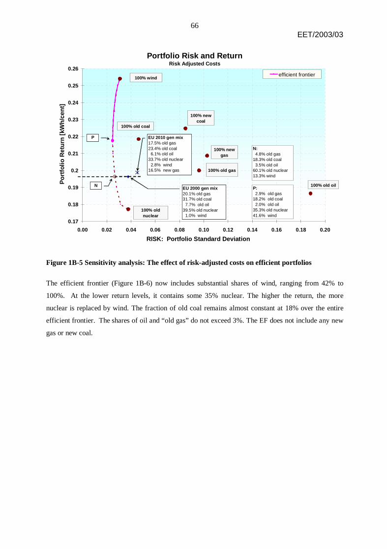
66EET/2003/03

Portfolio R isk and ReturnRisk Adjus ted Costs

0.17

0.18

0.19

0.2

0.21

0.22

0.23

0.24

0.25

0.26

0.00 0.02 0.04 0.06 0.08 0.10 0.12 0.14 0.16 0.18 0.20

RISK: Portfolio Standard Deviation

Po

rtfo

lio R

etu

rn [

kWh

/cen

t]

efficient frontier

100% old oil

100% old gas

100% old nuclear

E U 2000 gen mix 20.1% old gas 31.7% old coal 7.7% old oil 39.5% old nuclear 1.0% wind

100% wind

N

N: 4.8% old gas 18.3% old coal 3.5% old oil 60.1% old nuclear 13.3% wind

P

P: 2.9% old gas 18.2% old coal 2.0% old oil35.3% old nuclear 41.6% wind

100% newgas

100% new coal

100% old coal

E U 2010 gen mix17.5% old gas23.4% old coal 6.1% old oil33.7% old nuclear 2.8% wind16.5% new gas

Figure 1B-5 Sensitivity analysis: The effect of risk-adjusted costs on efficient portfolios

The efficient frontier (Figure 1B-6) now includes substantial shares of wind, ranging from 42% to

100%. At the lower return levels, it contains some 35% nuclear. The higher the return, the more

nuclear is replaced by wind. The fraction of old coal remains almost constant at 18% over the entire

efficient frontier. The shares of oil and “old gas” do not exceed 3%. The EF does not include any new

gas or new coal.

67EET/2003/03

Portfolio Mix Along the Efficient Frontier

0%

10%

20%

30%

40%

50%

60%

70%

80%

90%

100%

0.220

0.225

0.230

0.235

0.240

0.245

0.250

0.253

RETURN [kWh/cent]

SH

AR

E o

f ea

ch t

ech

nol

og

y

0.02

48

0.025

0

0.02

54

0.02

60

0.026

7

0.02

76

0.028

9

0.03

03

PORTFOLIO RISK

WIND

OLD COAL

OLD NUCLEAR

OL D GAS OL D OIL

Figure 1B-6 Sensitivity analysis of the portfolio mix along the efficient frontier using risk-adjusted costs

The recommendation based on this analysis is to move from EU-2000 to at least portfolio P because it

is the efficient mix that comes closest to it- although with higher return. P contains approximately 42%

wind, 35% nuclear and 18% “old coal”.

To sum up, using risk-adjusted costs has a major impact on the efficient frontier. It decreases the return

of P- the lowest possible return of the efficient frontier- from 0.275 kWh/cent to 0.218 kWh/cent (and

also of EU-2000 and EU-2010). The highest portfolio return attainable is 0.254 kWh/cent.

68EET/2003/03

Bibliography

Awerbuch Shimon, Estimating Electricity Costs and Prices: The Effects of Market Risk and Taxes.IEA Paris, forthcoming, 2002

Awerbuch, Shimon, [2000a] Investing in Photovoltaics: Risk, Accounting and the Value of NewTechnology,” Energy Policy, Special Issue, Vol. 28, No. 14 (November).

Awerbuch Shimon, [2000] Getting It Right: The Real Cost Impacts of a Renewables PortfolioStandard. Public Utilities Fortnightly, February 15, 2000

Awerbuch Shimon, [1995a] Market-Based IRP— It’s Easy! Electricity Journal, Vol. 6, No. 3 April,1995.

Awerbuch Shimon, [1995b] New Economic Cost Perspectives For Valuing Solar Technologies.Advances in Solar Energy, Vol. 10, ASES, edited by Karl W. Böer, 1995.

Awerbuch Shimon, The Surprising Role of Risk in Utility Integrated-Resource Planning, TheElectricity Journal, Vol. 6, No. 3, pp 20-33, April 1993

Bolinger M., Wiser R., Golove W., Quantifying the Value that Wind Power Provides as a HedgeAgainst Volatile Natural Gas Prices. LBNL-50484, June 2002

Brealey Richard A., Myers Stewart C., Principles of Corporate Finance. fourth edition, McGraw Hill,1991

Brower Michael C., Bell Kevin, Spinney Peter, Bernow Stephen, Duckworth Max, Evaluating the risk-reduction benefits of wind energy. Report to the US Department of Energy, Wind technologydivision, January 1997

Bureau of Labour Cost Statistics Data, US Employment cost index. http://www.bls.gov/data/ 2002

Copeland Thomas E., Weston J. Fred, Financial Theory and Corporate Policy. Third edition,Addison-Wesley, 1988

Duke Richard, Kammen Daniel M., The Economics of Energy Market Transformation Programs.Energy Journal, Vol. 20, No. 4, pp. 15-50, 1999

Electricity Information, OECD/IEA, France, Paris 2001

European Communities, Green Paper - Towards a European strategy for the security of energysupply. 2001

EPRI, Analysis of Risky Investments for Utilities. Final Report, Electric Power Research Institute,September 1983

ERU, ERU 11: Development and implementation of an advanced control system for theoptimal operation and management of medium size power systems with a largepenetration from renewable power sources. http://www.eru.rl.ac.uk/broch94/eru11.html,last accessed August 2002, 1995

ESA, EURATOM Supply Agency, Annual report 2000

Fama Eugene F., French Kenneth R., Value versus Growth: The International Evidence. Journal ofFinance, Vol. 53, pp.1975-1999, 1998

69EET/2003/03

Felder Frank, Hedging Natural Gas Price Risk by Electric Utilities. Master’s Dissertation, MIT Centerfor Energy Policy Research--Program in Technology and Policy, May 1994.

Ferderer J. Peter, Oil Price Volatility and the Macroeconomy, Journal of Macroeconomics, 18 1,Winter, pp. 1-26, 1996

Glynn Peter, Manne Alan, On the Valuation of Payoffs from a Geometric Random Walk of Oil Prices.Pacific and Asian Journal of Energy, Vol. 2, No. 1, pp. 47-48, 1988

Harlow W. V., Asset Allocation in a Downside-Risk Framework. Financial Analysts Journal, pp. 29-40, Vol. 47 (5), September-October 1991

Hassett Kevin, Metcalf Gilbert, Energy Conservation Investment: Do Consumers Discount the FutureCorrectly? Energy Policy, 21, pp. 710-716, June 1993

Helfat Constance E., Investment Choices in Industry. Massachusetts Institute of Technology (MIT),1988

Herbst Anthony, The Handbook of Capital Investing. Harper-Business, 1990

Hoff Thomas E., Integrating Renewable Energy Technologies in the Electric Supply Industry: A RiskManagement Approach, National Renewable Energy Laboratory (NREL), March 1997

Holt Richard, Boom and Bust: Chaos in Oil Prices, 1901-1987-- A Statistical Analysis. DC: USDepartment of Energy, Office of Technology Policy, 1988

Huber C., Haas R., Faber T., Resch G., Green J., Twidell J., Ruijgrok W., Erge T., Final Report of theProject ElGreen. Public Report of the Projet ElGrreen, Energy Economics Group (EEG), ViennaUniversity of Technology, Austria, 2001

Ibbotson Associates, Stocks, Bonds Bills and Inflation 1998 Yearbook, Chicago, 1998.

Ibbotson Roger, Sinquefield Rex, Stocks, Bonds, Bills, and Inflation: The Past and the Future.Charlottesville, Va.: Financial Analysts Research Foundation, 1982

IEA, Experience Curves for Energy Technology Policy. Paris 2000

IEA, World Energy Outlook, Paris, 2000

ILO, Occupational Wages around the World (OWW) Database. October Inquiry Databasewww.nber.org/oww, 2001

Kendall, Maurice, The Analysis of Economic Time Series. Journal of the Royal Statistical Society,Vol. 96, 11-25, 1953

Kwan Clarence C. Y. Portfolio Analysis Using Spreadsheet Tools. Journal of Applied Finance, No. 1,pp. 70-81, 2001

Markowitz Harry M., Portfolio Selection, Journal of Finance, Vol. 7, pp 77-91, March 1952

Papapetrou Evangelia. Oil price shocks, stock market, economic activity and employment in Greece.Energy Economics Vol. 23 (5), pp. 511-532, September 2001

Pethick David, Calder Rebecca, Clancy Chris, When the wind doesn’t blow. Energy Power RiskManagement, Vol. 6, No 12, March 2002

70EET/2003/03

Sadorsky Perry, Oil price shocks and stock market activity. Energy Economics 21, pp. 449-469, 1999

Sauter Raphael and Awerbuch Shimon, Oil Price Volatility and Macroeconomic Activity, A Surveyand Literature Review, Working Paper, IEA – REU, August, 2002

Seitz Neil, Capital Budgeting and Long-Term Financing Decisions. Dryden Press, 1990

Sharpe W, Portfolio Theory and Capital Markets, McGraw-Hill, Inc., 1970

Springer Urs, Laurikka Harri, Quantifying Risks and Risk Correlations of Investment in ClimateChange Mitigation, IWOe Discussion Paper No. 101, ISBN No. 3-906502-98-8, University of St.Gallen, October 2002

Stirling Andrew, Diversity and ignorance in electricity supply – Addressing the solution rather than theproblem, Energy Policy, Vol. 22, pp. 195-216, March 1994

Unger Georg, Strategische Produktionsplanung in der Pflanzenproduktion durch Portfolio-Selectionand Simulation, Dissertation, Vienna University of Economics and Business Administration, 1989

Venetsanos K., Angelopoulou P., Tsoutsos T., Renewable energy sources project appraisal underuncertainty: the case of wind energy exploitation within a changing energy market environment.Energy Policy, Vol. 30, pp. 293-307, 2002

Wind Energy Weekly, American Wind Energy Association, Vol. 15, #680,http://ces.iisc.ernet.in/hpg/envis/wwdoc1.html, last accessed August 2002, 15 January 1996

World Energy Outlook, OECD/IEA, personal communication, France, Paris 2000

Yang C. W., Hwang M. J., Huang B. N. An analysis of factors affecting price volatility of the US oilmarket. Energy Economics 24, pp. 107-119, 2002

© OECD/IEA, 2002

Applications for permission to reproduce or translate all or part of this publication should be made to:Head of Publications Service, OECD/IEA

2, rue André-Pascal, 75775 Paris cedex 16, Franceor

9, rue de la Fédération, 75739 Paris Cedex 15, France.