
IE304_LectureNotes_1
64
1 Manufacturing Models Manufacturing can be defined as a series of interrelated activities and operations involving the design, material selection, planning, manufacturing process, quality assurance, management and marketing of the products of the manufacturing industries. The goal is to produce products that meet customer expectations in terms of functionality, quality, and reliability BUT at a minimum cost. The industrial engineer determines how best to utilize the available inputs of labor, technology, capital, energy, materials and information to achieve the objectives.
-
Upload
oguzhan-oezdemir -
Category
Documents
-
view
213 -
download
1
description
ie304
Transcript of IE304_LectureNotes_1

1
Manufacturing Models
Manufacturing can be defined as a series of interrelated activities and
operations involving the design, material selection, planning,
manufacturing process, quality assurance, management and marketing of
the products of the manufacturing industries.
The goal is to produce products that meet customer expectations in terms
of functionality, quality, and reliability BUT at a minimum cost.
The industrial engineer determines how best to utilize the available inputs
of labor, technology, capital, energy, materials and information to achieve
the objectives.

2
Manufacturing Processes
INP
UT
S
Material
Labor
Information
Capital
Energy
Manufacturing Processes:
a) consist of physical
elements interacting
with each other
b) can be monitored via
performance measures
Products
Physical Elements
• Machinery
• Tools
• Computerized Equipment
• People
• Material Handling Equipment
Performance Measures
• Production rate
• % On-Time Delivery
• Defects per Million
• Unit cost

3
Transformation Process at a Food Processor
Inputs:
• Raw vegetables
• Metal Sheets
• Water
• Energy
• Labor
• Building
• Equipment
• Chemicals
• Coloring material
Processes:
• Cleaning
• Making Cans
• Cutting
• Cooking
• Packing
• Labelling
Outputs:
• Canned vegetables

4
Transformation Process at a Hospital
Inputs:
• Doctors
• Nurses
• Other personnel
• Building(s)
• Equipment
• Labs
• Medical supplies
Processes:
• Examination
• Surgery
• Monitoring
• Medication
• Therapy
Outputs:
• Treated patients

5
Products vs Services
Products:
• Tangible
• Can be stocked
• No interaction between customer
and process
Services:
• Intangible
• Cannot be stocked
• Direct interaction between
customer and process
Service industries have been on the rise and constitute most of the economy
in the Western world.

6
Manufacturing Systems
1. Product Design: blueprints, Computer-Aided Design
2. Process Planning:
• Sequence of operations to convert raw material into
finished goods
• Machine selection: Right equipment and tools to be able to process
parts according to design specifications
3. Production/Manufacturing Operations:
• Fabrication: Drilling a hole, plastic injection molding, bending a flange
• Assembly: Combination of separate parts into a more valuable
combined unit
4. Material Flow/Facilities Layout:
• Material Handling: Techniques for transporting parts, tools, scrap in
the facility
• Facility Layout: Placing production facilities, power supply,
compressed air within the facility
5. Production Planning/Control:
Use market demand, consider production capacity and current inventory
levels, determine planned production levels by product family.

7
Manufacturing Facility Layouts
There are four types of layouts:
1. Product Layout
2. Process Layout
3. Group Technology
4. Fixed Position (not to be covered)
The types of products in terms of their volume, variety dictate the layout. In
other words, these 4 layouts are not alternatives to one another.

8
How do We Assess and Characterize the Layout Types?
Throughput Time: The period required for a material, part, or subassembly to
pass through the manufacturing process.
Work in process (WIP): The set of items, parts and material for products not
completed. They are waiting in buffers (areas between workstations) for further
processing.
Skill level of workers
Product variety
Worker and machine utilization
Unit production cost
9
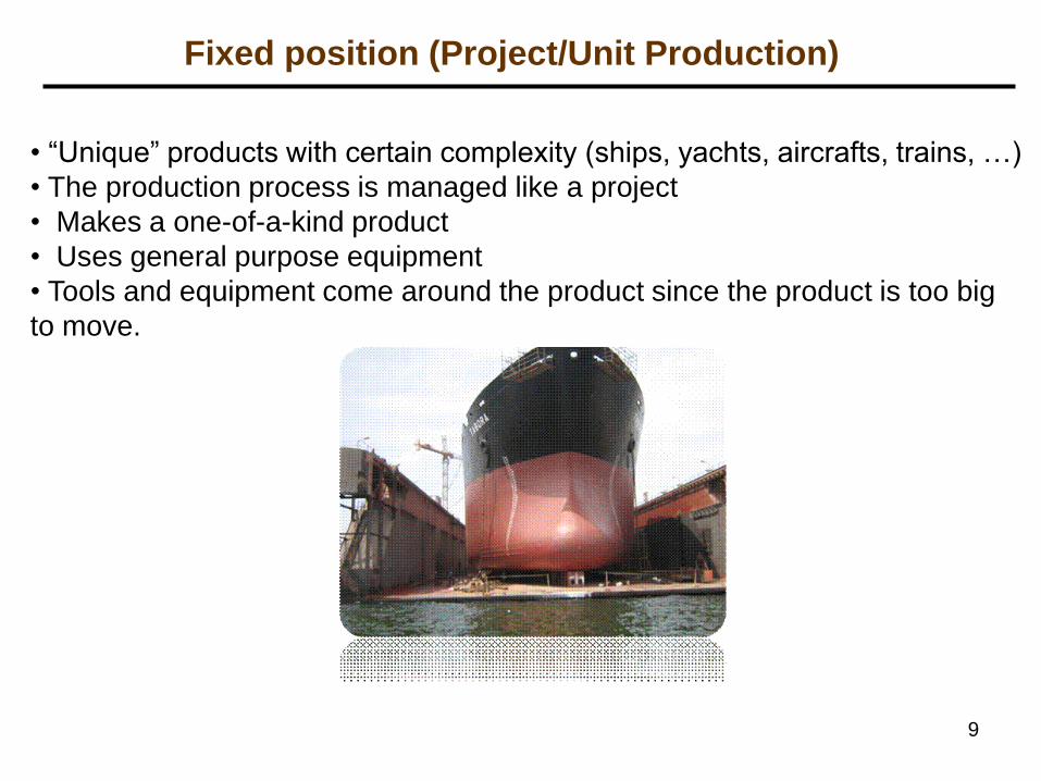
Fixed position (Project/Unit Production)
• “Unique” products with certain complexity (ships, yachts, aircrafts, trains, …)
• The production process is managed like a project
• Makes a one-of-a-kind product
• Uses general purpose equipment
• Tools and equipment come around the product since the product is too big
to move.

10
Product Layout (Mass Production/Flow Lines)
A layout structure designed to make discrete parts. Parts move
through a set of specially designed workstations at a controlled rate.
Characteristics:
1. Makes few products in large volume
2. Uses specialized high-volume equipment
3. Workstations and machines for production are specific for the
product, and cannot be easily adjusted to other products.
4. Short throughput time, low WIP (work-in-process) inventories
11
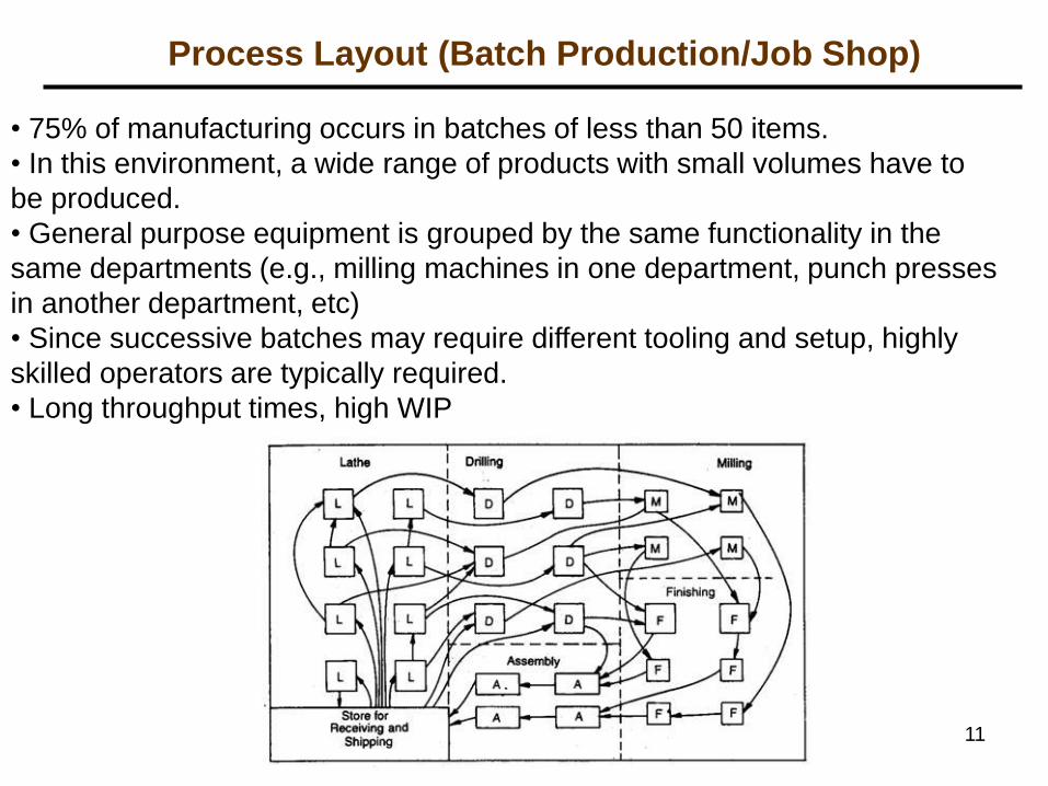
Process Layout (Batch Production/Job Shop)
• 75% of manufacturing occurs in batches of less than 50 items.
• In this environment, a wide range of products with small volumes have to
be produced.
• General purpose equipment is grouped by the same functionality in the
same departments (e.g., milling machines in one department, punch presses
in another department, etc)
• Since successive batches may require different tooling and setup, highly
skilled operators are typically required.
• Long throughput times, high WIP

12
• When there is a high variety of low demand products, if similar parts can be
grouped together in sufficient quantity, they are processed in a cell
• Different machines are placed in the same cell for similar parts
• Thus, scheduling and material handling are streamlined, low WIP and short
throughput time
Group Technology/Cellular Manufacturing

13
Comparison of Process Layout and Group Technology
14
Measuring Process Performance
• Productivity: Ratio of output to input
• Utilization: Ratio of the time that a resource is actually activated relative to
the time that it is available for use.
• Cycle Time: Average time between the completion of successive units.
• Run Time: Time required to produce a batch of parts.
• Setup Time: Time required to prepare a machine to make a particular item
• Operation Time: Sum of setup and run time.
• Throughput Rate: Number of parts processed per unit time.
• Value Added Time: Time that useful work is actually done

Assembly Lines
• Assembly operation: joins two or more components to create a
new entity, which is called an assembly, or subassembly.
• Assembly line: A production line consisting of a sequence of
workstations where assembly tasks are performed by human
workers or machines as the product moves along the line.
• Organized to produce a single product or a limited range of
products
– Each product consists of multiple components joined together by
various assembly work elements
15
16
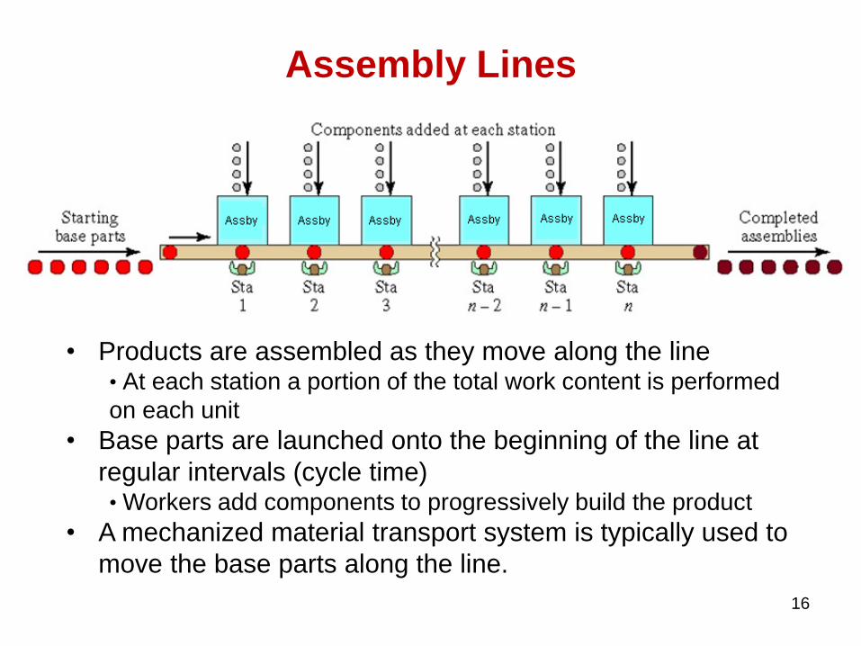
• Products are assembled as they move along the line • At each station a portion of the total work content is performed
on each unit
• Base parts are launched onto the beginning of the line at
regular intervals (cycle time) • Workers add components to progressively build the product
• A mechanized material transport system is typically used to
move the base parts along the line.
Assembly Lines

Assembly Lines
• Factors favoring the use of assembly lines:
– High or medium demand for product
– Identical or similar products
– Total work content can be divided into work elements
• Why assembly lines are so productive?
– Specialization (Division) of labor
• A large job is divided into small tasks and each task is assigned to one
worker
– Interchangeable parts
• Each component is manufactured to sufficiently close tolerances
– Work flow principle
• The work is moved to the worker
– Line pacing
• Workers are required to complete their assigned tasks on each unit within a
certain cycle time
• A specified production rate is maintained
17
Advantages
• Assembly lines reduced production cost and increased
production volume
• Keeps direct labor or automated machines busy doing
productive work
• Minimal setup times since the tasks are repeated
• Assembly lines do not require large queues, thus
• reduced WIP and lower inventory holding cost
• reduced space requirements
• shorter throughput time
18
Assembly Lines

Assembly Lines
• Most consumer products are assembled on assembly
lines
Automobiles Personal computers
Cooking ranges Power tools
Dishwashers Refrigerators
Dryers Telephones
Furniture Toasters
Lamps Trucks
Luggage Video DVD players
Microwave ovens Washing machines
19

Assembly Line Types
• Paced lines vs. Unpaced lines
Paced lines
o Each workstation is given exactly the same amount of time
(C, cycle time) to operate on a unit of product.
o At the end of C time units, the handling system
automatically indexes each unit to the next station.
o Encourages the workers to maintain the proper pace
o Randomness of performance may cause some items not to
be completed
o Extra time may be allowed
o Small buffers can be used to prevent starvation.
Unpaced lines do not have such restrictions.
New unit is removed from the handling system when the
previous one is completed
20
• Single product vs. Mixed lines
Mixed lines
o Used when single item types do not have sufficient demand
to justify an assembly line
o Several products are produced simultaneously
o Different workstations may process different productions at
the same time.
o Problems
• Scheduling the sequence of different products
• More complex line balancing problem
• Logistics - get the right parts for the models currently
processed in each workstation
21
Assembly Line Types
Fundamentals of Assembly Lines
• Assembly workstations
• Work Transport Systems
– Manual transport systems
– Mechanized transport systems
22

23
Workstation: A designated location along the work flow path at which one or more work elements are performed by one or more workers
Typical operations performed at assembly stations
Adhesive application
Sealant application
Arc welding
Spot welding
Electrical connections
Component insertion
Press fitting
Riveting
Snap fitting
Soldering
Stitching/stapling
Threaded fasteners
Assembly Workstations
• Manual transport methods
– Work units are moved between stations by the workers
without the aid of a powered conveyor
• Types:
– Work units moved in batches
– Work units moved one at a time
• Problems:
o Starving of stations – worker is available for the next unit, but
the unit has not yet arrived
o Blocking of stations – worker cannot pass the unit to the next
station since that worker is not ready yet
o No pacing – production rates tend to be lower
24
Work Transport Systems
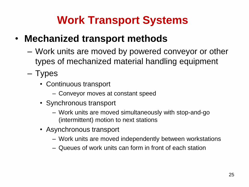
• Mechanized transport methods
– Work units are moved by powered conveyor or other
types of mechanized material handling equipment
– Types
• Continuous transport
– Conveyor moves at constant speed
• Synchronous transport
– Work units are moved simultaneously with stop-and-go
(intermittent) motion to next stations
• Asynchronous transport
– Work units are moved independently between workstations
– Queues of work units can form in front of each station
25
Work Transport Systems

26
Continuously moving conveyor operates at constant velocity
Can be implemented in two ways:
(1) work units are fixed to the conveyor
(2) work units are removable from the conveyor
Continuous Transport

27
All work units are moved simultaneously to their respective next
workstations with quick, discontinuous motion
The task must be completed within a certain time limit
Ideal for automated production lines
Synchronous Transport

28
Work units move independently, not simultaneously.
A work unit departs a given station when the worker releases it.
Small queues of parts are permitted to form at each station.
Forgiving of variations in worker task times.
Asynchronous Transport

29
Determination of the Cycle Time
• Production rate = 2200 units / week
• Number of working days / week = 5 days
• Number of shifts = 2 / day
• Number of hours / shift = 4 hours
• Breaks = 2*10 min / shift
• Net minutes per shift = ?
• Net minutes per week = ?
• C = ?
30
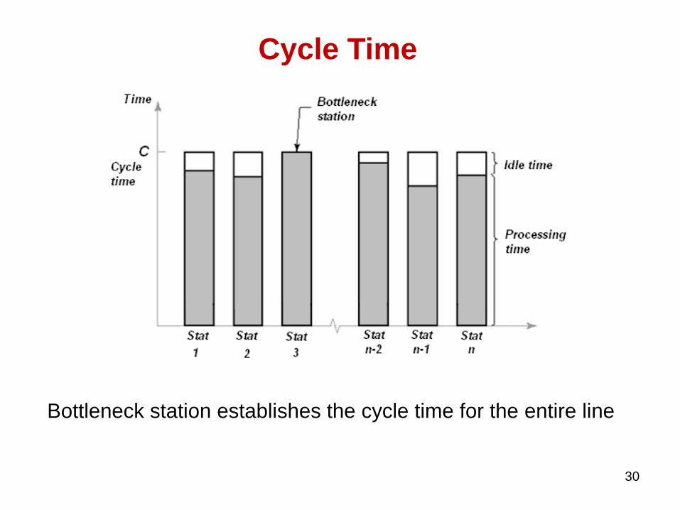
Cycle Time
Bottleneck station establishes the cycle time for the entire line

• Given:
– Total work content consists of many distinct work
activities
– The sequence in which the activities can be
performed is restricted
– The line must operate at a specified cycle time
• Problem:
– Assign tasks to the minimum number of stations
such that the workload assigned to each station does
not exceed the cycle time and the idle time is
minimized.
31
Line Balancing Problem

• C: cycle time
• n (possible) workcenters, m tasks
• ti : time to perform task i, i = 1,…,m
• Assume
– 𝐶 ≥ max𝑖{𝑡𝑖}
– 𝑛 ≥ 𝑡𝑖𝑚𝑖=1
𝐶
• 𝑐𝑖𝑗: cost of assigning task i to station j, i=1,…,m, j = 1,…,n
– To minimize the idle time force tasks into lowest numbered stations.
Assume 𝑚 𝑐𝑖𝑗 < 𝑐𝑖,𝑗+1, 𝑗 = 1,… , 𝑛 − 1
• Precedence constraints: IP
• Zone constraints: ZS and ZD
32
Line Balancing Problem - Formulation
necessary?

33
• Restrictions on the order in which work elements can be
performed
• IP = {(u,v): task u is an immediate predecessor of task v }
IP = ?
Precedence Constraints
Precedence
diagram

Zone Constraints
• Limitations on the grouping of tasks and/or their
allocation to workstations
– ZS: Positive zoning constraints
• Tasks should be grouped at same station
• Example: spray painting elements
ZS = {(u,v) | u and v must be assigned to the same station}
– ZD: Negative zoning constraints
• Elements that might interfere with each other
• Ex: Separate delicate adjustments from loud noises
ZD = {(u,v) | u and v cannot be assigned to the same station}
34

Problem Formulation
35

36
m
i
n
j
jiji xc1 1
,,min
m
i
jii njCxt1
, ,...,1 ,
Sum of task times of tasks assigned to each station cannot exceed cycle time
,...,m ixn
j
i,j 1 ,11
Each task must be assigned to exactly one station
h
j
juhv IPu,v ,n ,h,xx1
,, )(and 1
If task v is assigned to station h its immediate predecessor(s) u must be assigned to
some station between 1 and h
n
j
jvju ZSu,v,xx1
,, )( 1
u and v must be assigned to the same station
ZDu,v ,...,n j,xx jvju )(and 1 1,,
u and v cannot be assigned to the same station
Problem Formulation
,...,n j,x ji 1 and m,1,..., i }1,0{, xij is a binary variable
(LB - I)

37
Assign tasks to a fixed number of stations n such that the cycle time, C,
is minimized. This also maximizes the output rate.
m
i
jiij
xt1
,maxmin
s.t. ,...,m ix
n
j
i,j 1 ,11
h
j
juhv IPu,v ,n ,h,xx1
,, )(and 1
Assembly Line Balancing – Different Objective
n
j
jvju ZSu,v,xx1
,, )( 1
,...,n j,x ji 1 and m1,..., i }1,0{,
ZDu,v ,...,n j,xx jvju )(and 1 1,,

38
We formulate the problem as follows:
min
njCxtm
i
jii ,...,1 1
,
s.t.
C
Assembly Line Balancing – Different Objective
,...,m ixn
j
i,j 1 ,11
h
j
juhv IPu,v ,n ,h,xx1
,, )(and 1
n
j
jvju ZSu,v,xx1
,, )( 1
,...,n j,x ji 1 and m1,..., i }1,0{,
ZDu,v ,...,n j,xx jvju )(and 1 1,,
(LB - II)

• Three heuristics:
– Largest Candidate Rule
– Kilbridge and Wester Method
– Ranked Positional Weights Method
• Assume there is no zone constraints
• Assume only one worker will be assigned to
each station
39
Line Balancing Algorithms

(0) Arrange tasks in descending order according to their
processing times ti, consider the first workstation
(1) Assign tasks to the workstation by starting at the top of
the list and selecting the first task that
– satisfies precedence requirements and
– does not cause the total workload of the station to exceed C
When a task is assigned to the station, start from the
top of the list
(2) When no more task can be assigned to the station,
proceed to the next station
(3) Repeat steps 1 and 2 until all tasks have been assigned
40
Largest Candidate Rule

41
Largest Candidate Rule
• Production rate = 2200 units / week
• Number of working days / week = 5 days
• Number of shifts = 2 / day
• Number of hours / shift = 4 hours
• Breaks = 2*10 min / shift
Cycle time C = 1 min
Number of workstations ≥ 4
1 = 4

42
Largest Candidate Rule
Task
(i)
ti Preceded
by
3 0.7 1
8 0.6 3, 4
11 0.5 9, 10
2 0.4 -
10 0.38 5, 8
7 0.32 3
5 0.3 2
9 0.27 6, 7, 8
1 0.2 -
12 0.12 11
6 0.11 3
4 0.1 1, 2
Tasks are arranged

43
Largest Candidate Rule
Station Task ti Station Time
1
2 0.4
5 0.3
1 0.2
4 0.1 1.0
2 3 0.7
6 0.11 0.81
3 8 0.6
10 0.38 0.98
4 7 0.32
9 0.27 0.59
5 11 0.5
12 0.12 0.62
Tasks are assigned to stations
Task
(i)
ti Preceded
by
3 0.7 1
8 0.6 3, 4
11 0.5 9, 10
2 0.4 -
10 0.38 5, 8
7 0.32 3
5 0.3 2
9 0.27 6, 7, 8
1 0.2 -
12 0.12 11
6 0.11 3
4 0.1 1, 2
Tasks are arranged

44
Largest Candidate Rule
Assignment of tasks to workstations
Physical sequence of stations with assigned tasks
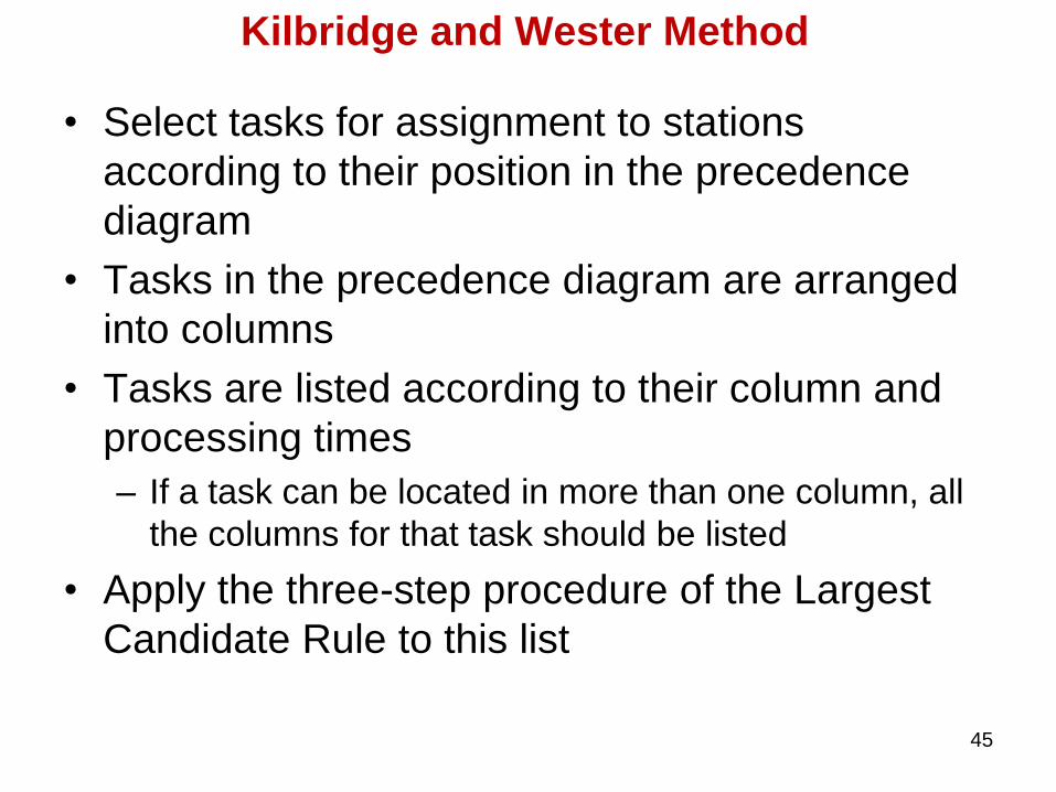
• Select tasks for assignment to stations
according to their position in the precedence
diagram
• Tasks in the precedence diagram are arranged
into columns
• Tasks are listed according to their column and
processing times
– If a task can be located in more than one column, all
the columns for that task should be listed
• Apply the three-step procedure of the Largest
Candidate Rule to this list
45
Kilbridge and Wester Method

46
Kilbridge and Wester Method
Task Column ti Preceded
by
2 I 0.4 -
1 I 0.2 -
3 II 0.7 1
5 II,III 0.3 2
4 II 0.1 1, 2
8 III 0.6 3, 4
7 III 0.32 3
6 III 0.11 3
10 IV 0.38 5, 8
9 IV 0.27 6, 7, 8
11 V 0.5 9, 10
12 VI 0.12 11
Tasks are listed according to their columns

47
Kilbridge and Wester Method
Station Task Column ti Station
Time
1
2 I 0.4
1 I 0.2
5 II 0.3
4 II 0.1 1.0
2 3 II 0.7
6 III 0.11 0.81
3 8 III 0.6
7 III 0.32 0.92
4 10 IV 0.38
9 IV 0.27 0.65
5 11 V 0.5
12 VI 0.12 0.62

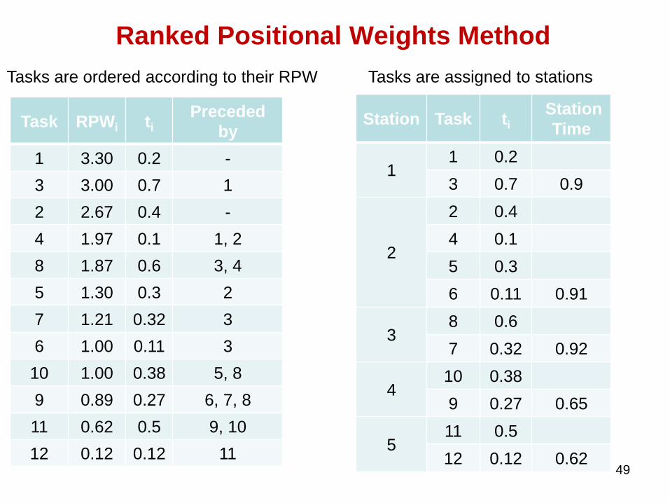
• Ranked positional weight of task i (RPWi):
𝑅𝑃𝑊𝑖 = 𝑡𝑗𝑗∈𝑉(𝑖)
𝑉(𝑖) is the set of all successors of node i (including i) in the
precedence diagram
• Compute the ranked positional weight of each task
• Order tasks according to their RPW value
• Apply the three-step procedure of the largest candidate
rule to this list
48
Ranked Positional Weights Method
49
Ranked Positional Weights Method
Task RPWi ti Preceded
by
1 3.30 0.2 -
3 3.00 0.7 1
2 2.67 0.4 -
4 1.97 0.1 1, 2
8 1.87 0.6 3, 4
5 1.30 0.3 2
7 1.21 0.32 3
6 1.00 0.11 3
10 1.00 0.38 5, 8
9 0.89 0.27 6, 7, 8
11 0.62 0.5 9, 10
12 0.12 0.12 11
Station Task ti Station
Time
1 1 0.2
3 0.7 0.9
2
2 0.4
4 0.1
5 0.3
6 0.11 0.91
3 8 0.6
7 0.32 0.92
4 10 0.38
9 0.27 0.65
5 11 0.5
12 0.12 0.62
Tasks are ordered according to their RPW Tasks are assigned to stations

• When only a small number of tasks are assigned to each station,
the idle time may be very high.
• Balance delay is a performance measure that represents the
proportion of idle time
• Example: C = 100 min, 3 tasks with task times 75, 50, and 70
min
– Assign each task to one station (n = 3)
– Balance delay is D = 0.35
Some Practical Issues (I)
Cn
tCn
D
m
i
i
1
50
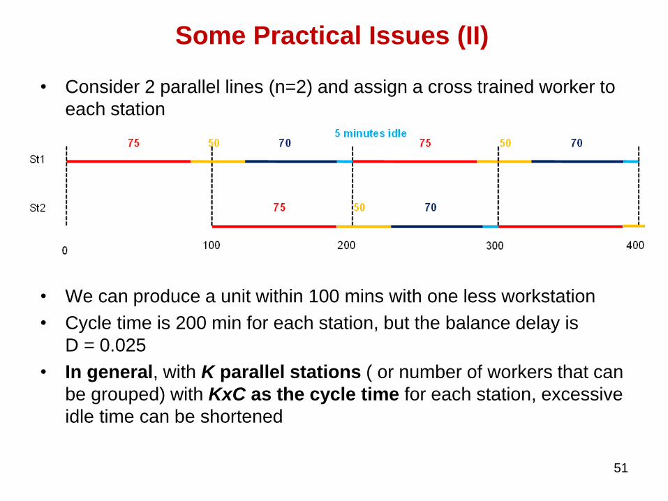
• Consider 2 parallel lines (n=2) and assign a cross trained worker to
each station
• We can produce a unit within 100 mins with one less workstation
• Cycle time is 200 min for each station, but the balance delay is
D = 0.025
• In general, with K parallel stations ( or number of workers that can
be grouped) with KxC as the cycle time for each station, excessive
idle time can be shortened
51
Some Practical Issues (II)
• If demand is uncertain and there is no idle time in the current line,
then we might need overtime or another shift.
• This is not a big problem for labor intensive lines.
• If, on the other hand, we have fixed equipment on the line, then a
different approach might be needed.
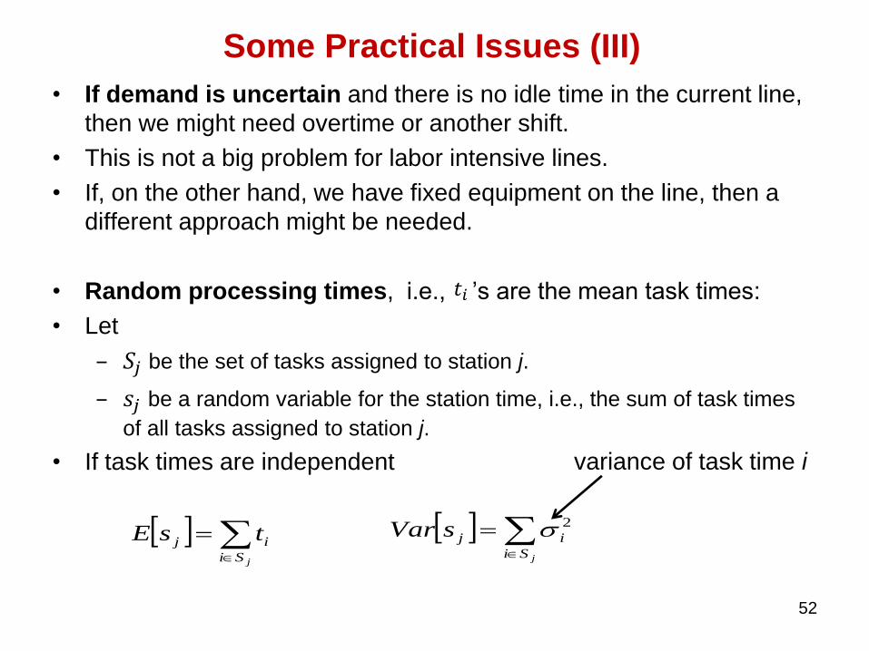
• Random processing times, i.e., ’s are the mean task times:
• Let
– 𝑆𝑗 be the set of tasks assigned to station j.
– 𝑠𝑗 be a random variable for the station time, i.e., the sum of task times
of all tasks assigned to station j.
• If task times are independent
52
Some Practical Issues (III)
𝑡𝑖
jSi
ij tsE
jSi
ijsVar 2
variance of task time i

• If each task time is normally distributed or we can invoke the
Central Limit Theorem, then 𝒔𝒋 is also normally distributed.
• If we require, e.g., 99% of the time to complete the assigned tasks in
each cycle at station j, then the following should hold:
𝐸 𝑠𝑗 + 2.33 𝑉𝑎𝑟[𝑠𝑗] ≤ 𝐶
• If all stations are created under this rule, the probability that ALL n
stations complete their tasks within C is 0.99𝑛
• In the case of random process times, we can assign utility workers
to help assembly workers in case of difficulty or provide for a rework
area where they can complete the unfinished tasks.
53
Some Practical Issues (IV)
54
Unpaced lines
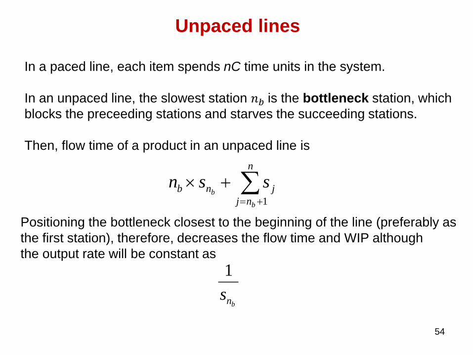
In a paced line, each item spends nC time units in the system.
In an unpaced line, the slowest station 𝑛𝑏 is the bottleneck station, which
blocks the preceeding stations and starves the succeeding stations.
Then, flow time of a product in an unpaced line is
n
nj
jnb
b
bssn1
Positioning the bottleneck closest to the beginning of the line (preferably as
the first station), therefore, decreases the flow time and WIP although
the output rate will be constant as
bns
1
55
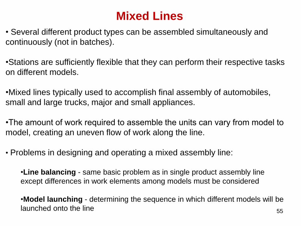
• Several different product types can be assembled simultaneously and
continuously (not in batches).
•Stations are sufficiently flexible that they can perform their respective tasks
on different models.
•Mixed lines typically used to accomplish final assembly of automobiles,
small and large trucks, major and small appliances.
•The amount of work required to assemble the units can vary from model to
model, creating an uneven flow of work along the line.
• Problems in designing and operating a mixed assembly line:
•Line balancing - same basic problem as in single product assembly line
except differences in work elements among models must be considered
•Model launching - determining the sequence in which different models will be
launched onto the line
Mixed Lines

56
Mixed Line Balancing
• There are P different products to be produced.
• 𝑅𝑗 is the production rate for product product j = 1,…,P
• 𝑡𝑖𝑗 is the necessary time for performing task i for product j,
i=1,…,m, j = 1,…,P
• Spread the workload amongst stations as evenly as possible.
• Compute the total time to perform each task
𝑇𝑇𝑖 = 𝑅𝑗𝑡𝑖𝑗𝑃𝑗=1 for 𝑖 = 1, … ,𝑚
• Assign the tasks to stations by using one of the line balancing
algorithms (Largest candidate rule, Kilbridge and Wester method,
Ranked positional weights method)
57
Mixed Line Balancing
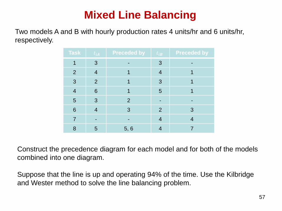
Task 𝑡𝑖𝑨 Preceded by 𝑡𝑖𝑩 Preceded by
1 3 - 3 -
2 4 1 4 1
3 2 1 3 1
4 6 1 5 1
5 3 2 - -
6 4 3 2 3
7 - - 4 4
8 5 5, 6 4 7
Construct the precedence diagram for each model and for both of the models
combined into one diagram.
Suppose that the line is up and operating 94% of the time. Use the Kilbridge
and Wester method to solve the line balancing problem.
Two models A and B with hourly production rates 4 units/hr and 6 units/hr,
respectively.

58
4
2
1
5
8 6 3
2
3
4
4 4
6 4
4
3
1
7
8 6 3
2
3
5
4
4
4 2
7
AB
4
1
5
8 6 3
2
AB
AB
AB
AB
A
B
AB
for model A
Precedence diagrams
for model B
for both models
Mixed Line Balancing
59
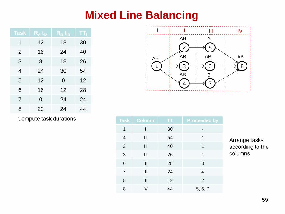
Mixed Line Balancing
Task RA tiA RB tiB TTi
1 12 18 30
2 16 24 40
3 8 18 26
4 24 30 54
5 12 0 12
6 16 12 28
7 0 24 24
8 20 24 44
7
AB
4
1
5
8 6 3
2
AB
AB
AB
AB
A
B
AB
I II III IV
Task Column TTi Proceeded by
1 I 30 -
4 II 54 1
2 II 40 1
3 II 26 1
6 III 28 3
7 III 24 4
5 III 12 2
8 IV 44 5, 6, 7
Compute task durations
Arrange tasks
according to the
columns

• Suppose that the line is up and operating 94% of the
time. Thus, the available time in one hour is
60min x 0.94 = 56.4 min
60
Mixed Line Balancing
Station Task TTi Station Time
1 1 30
3 26 56
2 4 54 54
3 2 40
5 12 52
4 6 28
7 24 52
5 8 44 44

• Determine the sequence of models and the time
difference between successive launches
• Two alternatives
– Variable-rate launching
• Time interval between successive launches is set equal to
the cycle time of that model
• The models can be launched in any sequence
• Causes logistical problems (supply of the correct
components to individual stations)
– Fixed-rate launching
• Time interval between two consecutive launches is constant
• The time interval depends on the product mix and production
rates of models
• Models must be launched in a specific sequence
61
Model Launching in Mixed Lines

Fixed-rate launching time interval is determined as
𝑇 = 1
𝑅 𝑅𝑗𝑇𝑗𝑃𝑗=1
𝑛
where
𝑅 = 𝑅𝑗𝑃𝑗=1 is the total production rate for all models
𝑇𝑗 = 𝑡𝑖𝑗𝑚𝑖=1 is the total time necessary for producing one unit of model j
𝑛 is the number of stations (or workers)
Let 𝐶𝑗 = 𝑇𝑗
𝑛 for j = 1,…,P
If model j is launched in position r, let 𝐶 𝑟 = 𝐶𝑖
For each launch position r, select j so as to minimize
𝐶 ℎ + 𝐶𝑗 − 𝑟𝑇
𝑟−1
ℎ=1
2
62
Model Launching in Mixed Lines
63
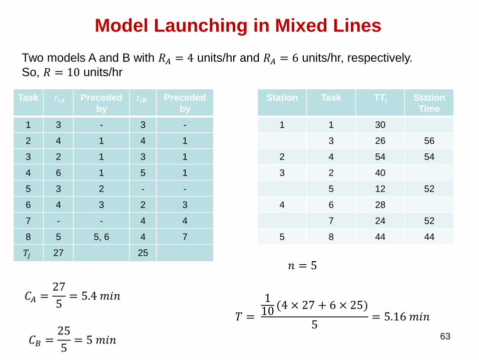
Model Launching in Mixed Lines
Task 𝑡𝑖𝐴 Preceded
by
𝑡𝑖𝑩 Preceded
by
1 3 - 3 -
2 4 1 4 1
3 2 1 3 1
4 6 1 5 1
5 3 2 - -
6 4 3 2 3
7 - - 4 4
8 5 5, 6 4 7
𝑇𝑗 27 25
𝐶𝐴 =27
5= 5.4 𝑚𝑖𝑛
Station Task TTi Station
Time
1 1 30
3 26 56
2 4 54 54
3 2 40
5 12 52
4 6 28
7 24 52
5 8 44 44
Two models A and B with 𝑅𝐴 = 4 units/hr and 𝑅𝐴 = 6 units/hr, respectively.
So, 𝑅 = 10 units/hr
𝑛 = 5
𝐶𝐵 =25
5= 5 𝑚𝑖𝑛
𝑇 =
110 (4 × 27 + 6 × 25)
5= 5.16 𝑚𝑖𝑛

Select the first launch
For model A, 5.4 − 1 × 5.16 2 = 0.0576
For model B, 5 − 1 × 5.16 2 = 0.0256
Select the second launch
For model A, 5 + 5.4 − 2 × 5.16 2 = 0.0064
For model B, 5 + 5 − 2 × 5.16 2 = 0.1024
64
Model Launching in Mixed Lines
Model B will be launched first
Set 𝐶 1 = 𝐶𝐵 = 5
Model A will be launched second
Set 𝐶 2 = 𝐶𝐴 = 5.4
Launch
(r) 𝐶 ℎ + 𝐶𝐴 − 𝑟𝑇
𝑟−1
ℎ=1
2
𝐶 ℎ + 𝐶𝐵 − 𝑟𝑇
𝑟−1
ℎ=1
2
Model
1 0.0576 0.0256 B
2 0.0064 0.1024 A
3 .1024 0.0064 B
4 0.0256 0.0576 A
5 0.16 0 B
6 0.0576 0.0256 B
7 0.0064 0.1024 A
8 0.1024 0.0064 B
9 0.0256 0.0576 A
10 0.16 0 B
The sequence is
B-A-B-A-B-B-A-B-A-B


