I.dtic.mil/dtic/tr/fulltext/u2/a455847.pdf · from the literature and with numerical simulations of...

Form ApprovedREPORT DOCUMENTATION PAGE OMB No. 0704-01-0188

1no puBlic reporting burden for trus collection aot Inlormatlon Is estimated to average 1 hour per response, Incluoing tHe time for reviewing Instruclions. searching ewsting Ctata sources, gatnenngand maintaining the data needed, and completing and reviewing the collection of informauton. Send comments regarding this burden estimate or any other aspect of this collection of information,Including suggestions for reducing the burden to Department of Defense, Washington Headquarters Services Directorate for Information Operations and Reports (0704-0188), 1215 JeffersonDavis Highway, Suite 1204, Arlington VA 22202-4302. Respondents should be aware that notwithstanding any other provision of law, no person shall be subject to any penalty for falling tocomply with a collection of Information if It does not displav a currently valid OMB control number.PLEASE DO NOT RETURN YOUR FORM TO THE ABOVE ADDRESS.

1. REPORT DATE (DD-MM-YYYY) 2. REPORT TYPE 3. DATES COVERED (From - To)

2002 Journal Article4. TITLE AND SUBTITLE 5a. CONTRACT NUMBER

Bioluminescence flow visualization in the ocean: an initial strategy based onlaboratory experiments 5b. GRANT NUMBER

5c. PROGRAM ELEMENT NUMBER

6. AUTHORS 5d. PROJECT NUMBERJim Rohr, Stewart Fallon'Mark Hyman2 S. TASK NUMBERMichael I. Latz

3

51. WORK UNIT NUMBER

7. PERFORMING ORGANIZATION NAME(S) AND ADDRESS(ES) 8. PERFORMING ORGANIZATION

'SSC San Diego 2Coastal Systems Station 3Scripps Institute of REPORT NUMBER

53560 Hull Street Code RI I Oceanography, UCSDSan Diego, CA 92152-5001 Panama City, FL 9500 Gilman Drive

32407-7001 La Jolla, CA 92093-02029. SPONSORING/MONITORING AGENCY NAME(S) AND ADDRESS(ES) 10. SPONSOR/MONITOR'S ACRONYM(S)

11. SPONSOR/MONITOR'S REPORTNUMBER(S)

12. DISTRIBUTIONAVAILABILITY STATEMENTApproved for public release; distribution'is unlimited.

13. SUPPLEMENTARY NOTESThis is the work of the United States Government and therefore is not copyrighted. This work may be copied and disseminatedwithout restriction. Many SSC San Diego public release documents are available in electronic format at:http://www.spawar.navy.millsti/publications/pubs/index.html

14. ABSTRACTObservations of flow-stimulated bioluminescence have been recorded for centuries throughout the world's oceans. The present study explores,within a laboratory context, the use of naturally occurring bioluminescence as a strategy towards visualizing oceanic flow fields. The response ofluminescent plankton to quantifiable levels of flow agitation was investigated in fully developed pipe flow. With two different pipe flowapparatus and freshly collected mixed plankton samples obtained over a year at two separate locations, several repeatable response patterns wereidentified. Threshold levels for bioluminescence stimulation occurred in laminar flow with wall shear stress levels generally between I and 2dyn cm-2 (0.1-0.2 N m-2), equivalent to energy dissipation per unit mass values of 102_103 cm 2s-3 (0-2.-10-Im 2s-3). In an attempt to account fordifferent concentrations and assemblages of mixed plankton, mean bioluminescence levels were normalized by an index of the correspondingflow-stimulated bioluminescence potential. This procedure generally accounted for variability between turbulent flow experiments, but was noteffective for laminar flow. In turbulent flow, mean bioluminescence levels increased approximately linearly with wall shear stress. Themagnitude of the flash response of individual cells, however, remained nearly constant throughout high laminar and turbulent flow, even as theenergetic length scales of the turbulence became less than the size of the organisms of interest. Threshold flow stimuli levels determined in thelaboratory were compared with oceanic measurements taken from the literature and with numerical simulations of ship wakes, one of the fewhighy turbulent flows to be well studied. Several oceanic flow fields are proposed as candidates for bioluminescence flow visualization.Published in Deep-Sea Research Part 1. Volume 49, pp. 2009-2033, 2002.

15. SUBJECT TERMSBioluminescence Laminar flowDinoflagellate Ship wake simulationFlow visualization Turbulent flow

16. SECURITY CLASSIFICATION OF: 17. LIMITATION OF 18. NUMBER 19a. NAME OF RESPONSIBLE PERSONa. REPORT b. ABSTRACT c. THIS PAGE ABSTRACT OF Jim Rohr, Code 2112I PAGES

19B. TELEPHONE NUMBER (Include area code)U U U UU 25 (619) 553-1604

Standard Form 298 (Rev. 8/98)Prescribed by ANSI Std. Z39.18

Available online at www.sciencedirect.com

SCIENCE~ DIRECTO EPSAISAC

PA~rr I

PERGAMON Deep-Sea Research I 49 (2002) 2009-2033www.elsevier.comlocate/dsr

Bioluminescence flow visualization in the ocean: an initialstrategy based on laboratory experiments

Jim Rohra, Mark Hymanb, Stewart Fallona'l, Michael I. Latzc,*,V 'SSC San Diego, 53560 Hull Street, D363, San Diego, CA 92152, USA

b Coastal Systems Station, Code RIl, Panama City, FL 32407-7001, USA

'Scripps Institution of Oceanography, University of California San Diego, 9500 Gilman Drive, La Jolla, CA 92093-0202, USA

Received 7 December 2001; received in revised form 23 July 2002; accepted 26 August 2002

Abstract

Observations of flow-stimulated biolumninescen;ce have' been 'recorded for 6enturi6s tlroughout the (,6rld's oceain§.The present study explores, within 'a laboriatory context, the use of naturally. occurring, bioluminescence a's a strategytowards visualizing oceanic flow fields. 'Theresponse 'of luminescent planktofi :t&6iitifiable levels of flow agitationwas investigated in fully developed pipe flow, With two different pipe' flow apparatus and freshly collected'mixedplankton samples obtained over a year at two separate locations, several repeatable response patterns were identified.Threshold levels for bioluminescence stimulation occurred in laminar flow with wall shear stress levels generallybetween I and 2dyncm- 2 (0.1-0.2 N m- 2), equivalent to energy dissipation per unit mass values of W02-10 3ci 2 s-3

(10-2_10-l m2 s- 3). In an attempt to account for different concentrations and assemblages of mixed plankton, meanbioluminescence levels were normalized by an index of the corresponding flow-stimulated bioluminescence potential.This procedure generally accounted for variability between turbulent flow experiments, but was not effective forlaminar flow. In turbulent flow, mean bioluminescence levels increased approximately linearly with wall shear stress.The magnitude of the flash response of individual cells, however, remained nearly constant throughout high laminarand turbulent flow, even as the energetic length. scales of the turbulence became less than the size of the organisms ofinterest. Threshold flow stimuli levels determined in the laboratory were compared with oceanic measurements takenfrom the literature and with numerical simulations of ship wakes, one of the few highly turbulent flows to be wellstudied. Several oceanic flow fields are proposed as candidates for bioluminescence flow visualization.Published by Elsevier Science Ltd.

Keywords: Bioluminescence; Dinoflagellate; Flow visualization; Laminar flow; Ship wake simulation; Turbulent flow; USA;California; San Diego Bay; Scripps Institution of Oceanography Pier

1. Introduction

*Corresponding author. Tel.: + 1-858-534-6579; fax: + 1- 1.1. Motivation

858-534-7313.E-mail address: [email protected] (M.I. Latz).

'Present address: Lawrence Livermore National Laboratory, There is no doubt that ship wakes can pro-Center for Accelerometer Mass Spectrometry, L-397 7000 East duce spectacular displays of bioluminescenceAvenue, Livermore, CA 94550, USA. (Harvey, 1952, 1957; Tarasov, 1956; Staples, 1966).

0967-0637/03/$ -see front matter Published by Elsevier Science Ltd.P11: S0967- 0637(02)001 16-4

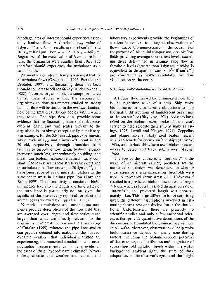
2010 J. Rohr et al. I Deep-Sea Research 149 (2002) 2009-2033

However, bioluminescence is also stimulated by and plant cells is dependent on the length scales ofmuch less energetic flows such as swell over the turbulence (reviewed by Hua et al., 1993).submerged bodies (Rohr et al., 1994), swimming Shear stress (viscous) and turbulent length anddolphins (Rohr et al., 1998), seals (Williams and time scales are also considered important para-Kooyman, 1985), small fish (Harvey, 1952), and meters for bioluminescence stimulation (Andersondivers (Lythgoe, 1972; Robinson, 1998). These et al., 1988; Widder et al., 1993; Latz et al., 1994;observations suggest that several energetic geo- Rohr et al., 1997). An experimental approachphysical flow fields may also be candidates for using fully developed pipe flow allows all thesebioluminescence flow visualization. Through de- flow parameters to be examined. Fully developedtermination of bioluminescence threshold levels in pipe flow is also advantageous because: it offers awell-characterized laboratory flow fields, geophy- wide range of laminar and turbulent flow stimuli,sical flow fields that are likely candidates for organisms experience the flow field for only a briefbioluminescence flow visualization can begin to be time period and are continuously replaced, andassessed within a scientific context. significant depletion of bioluminescence does not

occur in the upstream length of pipe (Losee and1.2. Background Lapota, 1981; Rohr et al., 1994).

Bioluminescence response patterns for mixedBioluminescence is one of the most cosmopoli- plankton samples (Rohr et al., 1997) and labora-

tan organism behaviors in the marine environ- tory cultures of the red-tide dinoflagellate Lingu-ment, having been found at all depths and in all lodinium polyedrum (Latz and Rohr, 1999) haveoceans of the world (Clark and Denton, 1962; been reported as a function of pipe wall shearWidder, 1997). In coastal waters, where opportu- stress, Twall, for predominantly laminar flows. Thenities to observe flow-stimulated bioluminescence present study examined the repeatability.of theseare typically best, the primary sources of biolumi- response patterns by testing freshly collectednescence are unicellular plankton called dinofla- mixed plankton at two different locations over agellates (e.g., Seliger et al., 1961; Kelly and Tett, year with the same pipe flow apparatus and1978; Morin, 1983; Lapota, 1998). It has been experimental approach. Because only a smallpostulated that concentrations <100 dinoflagel- range of turbulent flow has been 'previouslylates 1-1 are sufficient to highlight moving objects investigated (Rohr et al., 1997; Latz and Rohr,(Morin, 1983) and that visual predators use 1999), the effect of length and time scales of theflow-stimulated bioluminescence at night to locate turbulence on flow-stimulated dinoflagellate bio-their prey (Hobson, 1966; Mensinger and Case, luminescence is not known. The present study also1992; Fleisher and Case, 1995). Where extended used a larger pipe flow apparatus to obtain amonitoring of coastal bioluminescence has been greater range of turbulent length and time scales.conducted, abundances of bioluminescent dinoflagel- Throughout these experiments the homogeneity oflates were equal to or greater than 100 cells 1- (Kelly, mixed plankton abundance was assessed by1968; Lapota, 1998; Rapoport and Latz, 1998). periodic measurement of an index of the biolumi-During red tides, the abundance of luminescent nescence potential. These measurements provideddinoflagellates may reach 107 cells1-1 (Seliger et al., an opportunity to investigate whether mean1970). Thus, it appears that sufficient concentrations bioluminescence measurements obtained for dif-of bioluminescent dinoflagellates occur frequently ferent mixed plankton assemblages, but for theenough in coastal waters to provide opportunities, same flow stimuli, could be effectively scaled withwhen it is suitably dark, for nighttime oceanic flow an index of bioluminescence potential.visualization. Another important hydrodynamic feature is the

Some dinoflagellates are known to be very shear rate of energy dissipation per unit mass, hereaftersensitive (Thomas and Gibson, 1990a, b; Estrada referred to as the dissipation, e. Together with theand Berdalet, 1997; Juhl et al., 2000; Zirbel et al., kinematic viscosity, dissipation determines the2000). Generally, the shear sensitivity of animal Kolmogorov scales which are indicative of

J. Rohr et al. I Deep-Sea Research 1 49 (2002) 2009-2033 2011

the smallest length, LK, and time, LT, scales of the (1997) and Latz and Rohr (1999). It consisted of aturbulence. At small scales, instantaneous shear 91-cm long, 0.64-cm inner diameter (i.d.), trans-stress and dissipation are different descriptors of parent acrylic pipe connected to a 75-1 head tank.the same flow phenomenon, the deformation of A manual valve at the end of the pipe controlledthe fluid. The relationship between z and E depends the flow. Mean flow speeds up to 2.4m s-I wereon the flow field and author's preference, but has a achieved, providing maximum levels of viscouscommon form: stress at the pipe wall (Twall) of about 220 dyn cm-2

S = k(T) 2 (vp 2)- 1, () (=22Nm-2) (Table 1). The 0.64-cm i.d. pipe flowapparatus was used to investigate the response of

where v and p are the kinematic viscosity and freshly collected plankton samples obtained fromdensity of seawater, respectively, and k is a San Diego (SD) Bay and off the Scripps Institu-constant. For mathematical convenience k often tion of Oceanography (SIO) Pier, La Jolla, CA.appears as 21r in the oceanic literature (Mann and Between 30 May, 1994 and I 1 July, 1995, six 0.64-Denny, 1996). In fully developed laminar pipe cm i.d. pipe flow experiments with mixed planktonflow, k is indisputably. equal to one (Rosenhead, samples were performed at each location (Table 2).1963; Sherman, 1990). Assuming k = 1, Eq. (1) To obtain higher shear stresses, a pressurizedhas been used to study the effect of wind-induced pipe flow apparatus incorporating a 450-1 inertlyturbulence on dinoflagellate population growth coated stainless-steel head tank was assembled(Thomas and Gibson, 1990a), surfzone turbulence within an enclosure on a pier in SD Bay. Wateron purple sea urchin fertilization (Mead and was first drawn into a submerged tank through aDenny, 1995), and the biological consequences of 7.6-cm diameter, hydraulically actuated valvesmall-scale flow in a surge channel (Denny et al., located 2-3m below the sea surface. The sub-1992). Asimilar expression, but with k equal to merged tank was then gradually pressurized to10/it, has been employed by Latz et al. (1994) to slowly transfer the water into the head tank. Theestimate oceanic bioluminescence threshold dis- maximum shear stress during transport throughsipation- levels, using threshold shear stress values the 10-cm i.d. connecting hose was estimated asdetermined in simple laminar Couette flow. Lazier less than I dyn cm- 2. Mounted to the bottom ofand Mann (1989) suggest, based on the velocity the head tank was a 50-cm-diameter elbowshear spectra measured in a mixed layer (Oakey connected to a flange from which issued a 3-mand Elliot, 1980), that for most turbulent oceano- long, clear acrylic pipe of 0.85-cm i.d. Between thegraphic applications k = 7.5. For the present pipe and the flange was a smooth contracting inletoceanic comparisons a range of dissipation thresh- with a cubic polynomial profile. Through pressur-old levels was calculated from threshold shear izing the head tank and controlling a manual valvestress values determined in laminar pipe flow, at the end of the pipe, flow speeds in excess ofEq. (1), and k values of 1 and 7.5. Although 6ms-', with associated maximum "wall levelsthreshold dissipation and threshold shear stress around 1000dyn cm-2 , were attained (Table 1).values are not independent measurements, in the Six experiments were successfully conducted be-present study they are considered separately when tween 28 April, 1994 and 18 August, 1994 in thecompared to oceanographic shear and dissipation 0.85-cm i.d. pipe (Table 2). For comparison, anmeasurements. overlapping range of Twall values was measured for

both pipes. Each experiment for either apparatusconsisted of a single tank full of freshly collected

2. Experimental materials and methods seawater.Pressure drop, Ap, between the pressure taps

2.1. Pipe flow measurements separated by Ax along the pipe, was measured withvariable reluctance differential transducers (Vali-

The smaller pipe flow apparatus used in this dyne Corporation). Mean flow speed, Uavg, wasstudy was identical to that described by Rohr et al. calculated by dividing the volume flow rate by the


Table IRange of wall shear stress, ZTa,1, energy dissipation per unit mass, e, and Kolmogorov length, LK, and time, LT, scales (at centerline,LKý/I, LTC/l; averaged across the pipe diameter, LKavg, LTavg; and at the pipe wall, LKýaIl, LTwý1) for the pipe flow experiments

Pipe i.d. (cm) Laminar flow Turbulent flow

"%wall B~all Twall 8

wall LKc/I LKavg LKwall LTc/I LTa-g L'rwii

(dyn cm- 2) (cm 2 s-3) (dyn cm-2) ( 1 l06 cm

2 S-3) (Pim) (gsm) (Psm) (As) (Ws) (lAs)

0.64 0.2-29 3.6-76000 61-220 0.3-4.3 25-14 22-13 14-7 610-190 470-170 180-490.85 0.3-8 8.2-5800 20-1000 0.03-91 44-8 37-8 25-3 1800-26 1300-30 570-1I

Table 2Mixed plankton, bioluminescence pipe flow results. Mean slope is based on the least-squares regression of log mean bioluminescencevs. log Twal., with number of measurements in parentheses and r2 values in brackets

Experiment Threshold Twall (dyncm- 2) Mean slope

Location and date Laminar Turbulent

SD Bay 0.64-cm i.d5/30/94 1.4 2.1 (18) [0.97]6/02/94 1.1 1.8 (14) [0.96]7/06/95 1.3 2.1 (13) [0.9917/07/95 1.1 1.8 (20) [0.98]7/11/95 1.1 1.4(13) [0.93]7/18/95 1.7 2.0 (14) [0.97]Pooled data 1.3 +0.26 1.9±0.28

SIO Pier 0.64-cm i.d7/11/94 0.9 1.8 (13) [0.96]7/13/94 0.6 1.3 (10) [0.83]8/08/94 0.7 1.5 (9) [0.95]9/07/94 0.7 1.7 (21) [0.94]4/14/95 1.2 2.2 (27) [0.93]4/27/95 1.2 2.2 (22) [0.93]Pooled data 0.9 ±0.25 1.8 ±0.34

SD Bay 0.85-cm i.d Spring 19944/28/94 1.2 2.5 (8) [0.94] 0.9 (10) [0.96]5/01/94 0.7 2.1 (12) [0.95] 0.9 (17) [0.96]5/09/94 0.7 1.7 (9) [0.76] 1.3 (28) [0.98]5/10/94 0.6 1.9 (12) [0.76] 1.2 (13) [0.931Pooled data 0.8 +0.25 2.0+0.37 1.1 ±0.21

SD Bay 0.85-cm i.d. Summer 19947/27/94 0.8 1.7 (8) [0.66] 1.1 (14) [0.93]8/18/94 1.0 2.0 (5) [0.991 0.9 (06) [0.98]Pooled data 0.9+0.16 1.9±0.20 1.0±0.19

pipe cross-sectional area. The volume flow rate number, a dimensionless flow rate, were calculatedwas determined by weighing the flow discharge (Schlichting, 1979) for each bioluminescence mea-collected over a measured time. Darcy friction surement as previously described (Latz and Rohr,factor, a dimensionless pressure, and Reynolds 1999). Their relationship clearly marks where the

J. Rohr et at. I Deep-Sea Research 149 (2002) 2009-2033 2013

104 ?(formerly Gonyaulax polyedra; 40 jim in diameter),"Ceratium fusus (340 x 30 lim, length and width,

021 respectively) and Protoperidinium spp.r (70 x 60 gim). When mechanically stimulated until"= l0bioluminescence is depleted, L. polyedrum, C. fusus

,, and Protoperidinium spp. produce 1-2 x 108 (Bigg-0 4ley et al., 1969; Latz and Lee, 1995), 3-5 x 108

0 (Esaias et al., 1973; Sullivan and Swift, 1994) and

0.5-3 x 109 (Lapota et al., 1989; Swift et al., 1995)

t°2 ... 104 10 5 photons cell-', respectively.

Reynolds Number These particular luminescent dinoflagellates arecommon to the coastal waters off • southern

Fig. 1. Representative measurements of Darcy friction factor California (e.g., Sweeney, 1963; Holmes et al.,and Reynolds number. The dashed line is the theoreticalrelationship for laminar flow; the solid line is the accepted 1967; Kimor, 1983; Lapota, 1998). Although theempirical relationship for turbulent flow (Schlichting, 1979). most abundant dinoflagellate, L. polyedrum, isClosed traingles are data collected from the 0.64-cm i.d. pipe; motile (Kamykowski et al., 1992), its swimming isopen circles are data collected from the 0.85-cm i.d. pipe. weak compared to the flows considered through-

out this study. Like most bioluminescent dino-flow was laminar, turbulent, or transitional, and flagellates, L. polyedrum exhibits a circadianwhether the measurements were obtained in fully rhythmicity with emission one to two orders ofdeveloped pipe flow. The break between the data magnitude greater at night than during the day(Fig. 1) represents the region of transition from (Biggley et al., 1969; Sweeney, 1981). Dinoflagel-laminar to turbulent flow. lates typically respond to mechanical stimulation

The shear stress in fully developed pipe flow, within 20ms with a light flash of 100 ms or more inregardless of whether the flow is laminar or duration (Eckert, 1965; Widder and Case, 1981;turbulent, increases linearly from zero at centerline Latz and Lee, 1995).to a maximum at the pipe wall (Schlichting, 1979). For the 0.64-cm i.d. pipe flow experiments,The wall shear stress in fully developed pipe flow is surface seawater was collected by bucket from SDdirectly calculated from either measurements of Bay and off the SIO Pier, 2 h before sunset whenpressure drop or average flow rate (Schlichting, dinoflagellate bioluminescence is minimally exci-1979). table (Biggley et al., 1969). At dusk, the apparatus

In turbulent pipe flow, e decreases rapidly with was covered with opaque sheeting and experimentsdistance from the pipe wall (Laufer, 1954). commenced 2.5h later, when maximal levels ofEstimates of 8 at the pipe wall (Eq. (1); k = 1), bioluminescence are expected (Biggley et al., 1969).centerline (Davies, 1972), and averaged across the For the 0.85-cm i.d. pipe flow experiments, thepipe (Bakhmeteff, 1936) were made, and the organisms were drawn from an underwater re-corresponding values of the Kolmogorov length servoir 2 h before sunset and were immediately(LKwaII, LKc/I, LKavg) and time (Lrwall, LTC/b LTavg) introduced into an opaque head tank. Measure-scales were calculated (Tennekes and Lumley, ments commenced 2.5 h after sunset.1972). Kolmogorov length and time scales variedbetween 1 (3-39 pm) and 2 (11-1300 js) orders of 2.3. Bioluminescence measurementsmagnitude, respectively (Table 1).

Bioluminescence was measured with photon-2.2. Luminescent organisms counting photomultiplier (PMT) detectors as

described by Latz and Rohr (1999). MeanThe luminescent organisms identified in the pipe bioluminescence was calculated by averaging each

flow samples obtained throughout this study were data record and was expressed as counts s-'. PMTexclusively dinoflagellates, primarily L. polyedrum pulses were also counted in 5-ms time bins to


resolve individual flash events. Maximum biolu- values were calculated by substituting thresholdminescence was determined by taking the highest Twall into Eq. (1) with k = I and 7.5.5-ms integration value in each time series and was Background mean bioluminescence levels wereexpressed as counts 5ms-l. Maximum biolumi- measured with no flow and were composed ofnescence measurements serve as an indicator of the electronic noise, ambient light leakage, and spon-peak intensity of an individual flash (Rohr et al., taneous bioluminescence (of which only the last1997; Latz and Rohr, 1999). parameter will depend on cell concentration).

The same PMT was used for all the pipe flow Mean and maximum background levels forbioluminescence measurements, and was mounted both PMT's were usually within 40-60 and67cm from the inlet of the 0.64-cm i.d. pipe and 10-30counts 5ms-1, respectively, throughout all2.36m from the inlet of the 0.85-cm i.d. pipe. The the experiments. A representative mean back-PMT was coupled to the pipe with a light-shielded ground level of 45countss-I was chosen foradapter and viewed the entire pipe diameter and a determining threshold Ewal levels. Results werepipe length of 5 cm. A reference PMT, used for the largely insensitive, within a factor of 2, to the exact0.85-cm i.d. pipe flow experiments,' was mounted choice of PMT background level.to the quartz window opposite a 25.5-ml viewing For consistency, all bioluminescence measure-chamber of a flow agitator (described in Section ments were expressed as emission per time. This is2.4). Simultaneous pipe flow bioluminescence the most meaningful way to present responsemeasurements obtained with both PMTs mounted threshold and maximum intensity. However,opposite to each other showed that their sensitiv- measurements of flow-stimulated, mean biolumi-ities were within a few percent. Each PMT record nescence are often expressed as emission perwas obtained at a constant flow rate, providing a volume (Widder et al., 1993; Latz et al., 1994;fixed Twall for periods typically between 20 and Widder, 1997). This particular representation100s. The longer time series were collected for the attempts to account for advective effects that areslower flow rates so that flow volumes for all the most pronounced when the residency time of thetime series were approximately equal. A sampling flash within the view of the detector is longduration of 100s for the low flow rates was compared to its duration (Seliger et al., 1969;adequate for detection of the response threshold Widder et al., 1993; Widder, 1997). Extending the(Latz and Rohr, 1999). Neutral density filters were mathematical analysis for bathyphotometers (Se-used to attenuate the photon input to ensure that liger et al., 1969; Widder et al., 1993) to fullybioluminescence was never saturating the PMT. developed pipe flow, Rohr et al. (1994) derived a

A response threshold was calculated for each relationship between mean intensity, flash kineticspipe flow experiment by a method similar to that and organism residency times. Applying thisof Latz and Rohr (1999). First, for each of analysis throughout the present range of Twall forthe three pooled data sets (i.e., SIO Pier, 0.64-cm both the 0.64- and 0.85-cm i.d. pipe flow experi-i.d. pipe; SD Bay, 0.64-cm i.d. pipe; and SD Bay, ments, an approximate linear dependence on0.85-cm i.d. pipe) a range of laminar flows was advection was found for both pipes. Consequently,identified by eye, based on a trend for increasing log mean bioluminescence vs. log TwaI trends formean and maximum bioluminescence intensities the 0.64- and 0.85-cm i.d. pipes can be directlywith increasing T wall. Then, for each of the pipe compared because the effect of advection isflow experimental data sets, a least-squares regres- similar. Least-squares regressions of log meansion of log mean bioluminescence vs. log wall bioluminescence vs. log Twall were used to calculateshear stress was calculated throughout this range. slopes (mean +standard deviation) and r2 values.Threshold Twall values were determined from thisregression equation to calculate where the regres- 2.4. Homogeneity and bioluminescence potentialsion line intercepted background mean biolumi-nescence levels (Latz and Rohr, 1999). A The lack of homogeneity of bioluminescentcorresponding range of threshold dissipation organisms throughout the head tank can have as

J. Rohr et al. / Deep-Sea Research 149 (2002) 2009-2033 2015

much, or more, of an effect on bioluminescence partly corroborated by the fact that at sufficientlyintensity as changes in the level of flow agitation. high flow rates, the details of the agitator chamberThrough "gentle" pre-stirring of the 75-1 head design (Losee et a]., 1985), the length of upstreamtank, differences in cell abundance between section preceding the agitator (Losee and Lapota,samples collected at the end of the 0.64-cm- 1981), and the flow rate (Latz and Rohr, unpub-diameter pipe were typically less than 30% lished observations) do not significantly affectthroughout an experiment. Previous tests have bioluminescence measurements within the agitator.shown that "gentle" pre-stirring, which did not The flow agitator was attached to a 3.23-mstimulate bioluminescence, had no significant length of 2.54-cm i.d. pipe, which ran parallel toeffect on the hydrodynamic agitation threshold the 0.85-cm i.d. pipe. Between the 2.54-cm i.d. pipefor bioluminescence (Latz and Rohr, 1999). To and the flange of the head tank was a smoothtest for cell homogeneity in the pre-stirred 75-1 contracting inlet with the same cubic polynomial

.head tank, bioluminescence measurements were profile as the other pipes. The volume flow ratefirst collected for flow rates that proceeded in a through the agitator was consistent with shipboarddecreasing sequence and then an overlapping, photometer protocol, always greater than 0.3 1s-.increasing sequence. An experiment was rejected Six of the nine 0.85 i.d. pipe flow tests conductedonly if similar flow rates did not produce similar satisfied both criteria of repeatability for increas-bioluminescent intensities. Based on this criterion, ing and decreasing flow rates and approximatelyall 12 pre-stirred, 0.64-cm i.d. pipe experiments constant bioluminescence potential index through-were acceptable for further analysis. out the experiment. These six experiments were

The 450-1 pressurized head tank, which could further analyzed.not be pre-stirred, was subject to larger fluctua-tions in cell concentration during an experiment.Therefore, in addition to comparing mean biolu- 3. Computational methodsminescence measurements for overlapping increas-ing and decreasing flow rates, an index of the Some of the most comprehensive numericalflow-stimulated bioluminescence "potential" was simulations presently available for highly energeticmeasured periodically throughout each of the flow fields in the ocean are for the wakes of naval0.85-cm i.d. pipe flow experiments. Biolumines- ships (Rood, 1995). The objective of the presentcence potential indices were obtained with a flow study was not to use bioluminescence to detectagitator taken from a shipboard photometer ship wakes per se, but to demonstrate howsystem (Losee and Lapota, 1981; Losee et al., luminescent "footprints" could be predicted in1985; Lieberman et al., 1987). The flow agitator is turbulent oceanic flows. As numerical simulationscomposed of a 25.5-ml cylindrical chamber of 2.0- evolve, bioluminescence associated with highlycm radius and 2.0-cm height, with quartz windows energetic geophysical flows can be estimated.attached to its sides for viewing. The chamber's Numerical simulations were used to estimate thecylindrical axis is oriented perpendicular to the temporally and spatially averaged turbulent shearaxis of the pipe. The inlet i.d. of the chamber stress and energy dissipation fields throughout thereduces from 2.54 to 1 cm over a distance of wake of an aircraft carrier. These computations2.5 cm. The outlet from the chamber is a mirror were then used to delineate where within the wakeimage of the inlet. Because of the highly turbulent several candidate threshold values of turbulentflow stimulus within the flow agitator, the asso- shear stress and energy dissipation were attainedciated bioluminescence measurements are assumed or exceeded. The simulated aircraft carrier hadto serve as an effective index of the biolumines- four 6.4-m diameter propellers, a displacement ofcence potential, i.e., the maximum biolumines- 9.1 x 104 tons, and at waterline a length, beam andcence intensity that can be hydrodynamically draft of 332.5, 40.2 and 11 m, respectively. Thestimulated (Losee and Lapota, 1981; Losee et al., simulation was for a typical speed of 9m s-,1985; Lieberman et al., 1987). This presumption is about 18 knots.


The algorithm used to compute the wake flow Irrespective of these difficulties, it is believedfield, a parabolic Reynolds-averaged Navier- that the numerical simulation estimates of turbu-Stokes solver, is well-documented and has been lent shear stress and energy dissipation are relatedpartially verified with full-scale experiments on to the local flow properties responsible formany classes of US naval surface craft (Hyman, bioluminescence stimulation. The appropriate1990, 1992, 1994). For this initial assessment transfer functions can be derived given suitableof ship wake bioluminescence signatures, the field observations.effect of rising bubbles on modifying the flowfield was ignored. Because rising bubbles canstimulate luminescent plankton (Anderson et al., 4. Experimental results1988; Latz and Case, unpublished observa-tions), the bioluminescent "footprints" predicted 4.1. SD Bay and SIO Pier, 0.64-cm i.d. pipe flowby the present simulations are thought to be bioluminescence measurementsconservative.

Note that the turbulent or Reynolds shear stress Mean and maximum bioluminescence trendscalculated in the numerical simulations is funda- for the 0.64-cm i.d. pipe flow experiments withmentally different than the threshold shear stress mixed plankton collected from SD Bay (six experi-determined in laminar pipe flow. The turbulent ments) and off the SIO Pier (six experiments)length scales that dominate the Reynolds stresses were generally in good agreement (Fig. 2A and B;tend to be the larger length scales of the flow Table 2). With increasing laminar flow, mean(Stacey et al., 1999b). The smallest length scales in and maximum bioluminescence normally in-the simulations are many orders of magnitude creased above background levels in flows withgreater than the bioluminescent dinoflagellates of Twail around I dyncm-2. For the range ofinterest. The distance between grid points varied Twall = 1-29dyncm- 2 in laminar flow, the in-from tens of centimeters at the free surface and crease in mean bioluminescence as the 1.9+0.3centerline to tens of meters at the subsurface edges power of rwall for the six SD Bay experiments wasof the wake. not significantly different from the increase as the

In principle, for large Reynolds number flows 1.8+0.3 power for the six SIO Pier experimentssuch as full-scale ship wakes, dissipation at the (t = 0.045; d.f. = 10; P = 0.66). Pooling all laminarscales of luminescent plankton can be reliably flow data for the two locations, mean biolumines-discerned from measurements at much larger cence increased as the 1.8+0.3 power of Twall

scales (Tritton, 1988). Unfortunately, except for (r2 = 0.89; n = 194). In turbulent flow, the rela-a Direct Numerical Simulation, dissipation is the tively small logarithmic range of Twa5 j betweencomputed quantity with the largest uncertainty. 62 dyn cm- 2 and 218 dyn cm- 2 and large scatter inBecause there are no direct measurements of the mean bioluminescence data precluded thedissipation in a ship's wake, simulations must be identification of a meaningful power-law relation-checked indirectly, usually through another vari- ship.able that is better understood and accurately Pooling all SD and SIO 0.64-cm i.d. pipe flowmeasured. In the present case, the initial value of data from the two locations, the response thresh-dissipation was derived from a length scale old occurred in flows with a Twall ofproportional to the propeller diameter, which 1.1 + 0.3 dyn cm- 2 . The corresponding Twall thresh-was determined by optimizing the comparison of old values for the SD Bay and SIO Pier experi-computations against a limited set of wake data ments were 1.3+0.2 and 0.9+0.2dyncm- 2 ,taken in a tow tank (Swean, 1987). In subsequent respectively. Although as order of magnitudesimulations, while the near wake was fairly estimates these thresholds levels were remarkablysensitive to dissipation error, most far-wake similar, they were significantly different at the P =

simulations were not, apparently tending towards 0.02 level (t = 2.746; d.f. = 10). Comparing 1994a self-similar structure. and 1995 measurements, there was no difference in

I Rohr et al. I Deep-Sea Research 149 (2002) 2009-2033 2017

106

0 104

103

• 102

101 ..... I ,. , , , . I I

(a) 0.1 1 10 100 1000

105 30

104

LA La 20 u

• Go

10 0

100 .,, .. , ,..I0

0.1 1 10 100 1000

(b) Wall Shear Stress (dyn cm-2 )

Fig. 2. Luminescent response of mixed plankton samples tested in the 0.64-cm i.d. pipe apparatus. Samples were collected from SDBay (closed symbols) and SIO Pier (open triangles) over 1 year (Table 2). Each symbol indicates the result for one flow rate. Dashedlines represent the background level in the absence of flow. (A) Mean intensity as a function of wall shear stress. (B) Maximumintensity as a function of wall shear stress. The solid line indicates the Kolmogorov turbulent length scale, which is related to thesmallest length scales of the turbulence. The smallest luminescent plankton present, Lingulodinium polyedrum, are about 40 Ptm indiameter. The gap in the data between Ta1 of 29-64dyn cm- 2 is the region where transition from laminar to turbulent flow occurred.

threshold Twall values for the two locations 4.2. SD Bay, 0.85-cm i.d. pipe flow bioluminescence(t = 0.471; d.f. =4; P = 0.66) in 1995, but in 1994 measurementsthere was a significant difference (t = 3.986;d.f. = 4; P = 0.02) due to a lower threshold of Throughout laminar flow, mean and maximum0.7 + 0.1 dyn cm- 2 at the SIO Pier location, bioluminescence of SD Bay water samples tested in

Maximum bioluminescence measurements ex- the 0.85-cm i.d. pipe apparatus increased as ahibited greater variability than mean biolumines- function of twall (Figs. 3A and B; Table 2) in acence, particularly near threshold (Fig. 2B), similar way as was found for the 0.64-cm i.d. pipebecause of the reduced statistical likelihood of (Figs. 2A and B; Table 2). There was no significantobserving the relatively short (,: 10ms) temporal difference in twall threshold (t = 0.471; df=4;peak of an individual flash. With increasing P=0.66) and mean slope (t=0.735; d.f.=4;laminar flow, maximum bioluminescence measure- P = 0.50) between spring and summer 1994ments for all the 0.64-cm i.d. pipe flow experiments measurements in the 0.85-cm i.d. pipe. Thefirst increased more than two orders of magnitude bioluminescence stimulation threshold for thebetween threshold and Twall values of 10 dyn cm-2, pooled data occurred in laminar flows withand then remained nearly constant through T wall = 0.8+0.2dyncm- 2. Although some of thetransition from laminar to turbulent flow. mean bioluminescence data for T wall < 1 dyn cm-2


were above background, these data were not 106

included for threshold calculations due to the .poor correlation between mean bioluminescence 0and Twall throughout this range. For laminar flows o ,0with twali between 1-10dyncm 2 , spring andsummer pooled mean bioluminescence intensityincreased as the 2.0+0.3 power of Twall. For 0 2 o 0turbulent flow there was a dramatic difference in -609.... -- - - -

mean bioluminescence intensity between spring (a) 1°:0.1 10 100 10.on

and summer (Fig. 3A). However, there was nosignificant difference in the mean slope (t = 0.451; 1o 30

d.f. = 4; P = 0.68). For turbulent flows with T'wall . oO• o 25

values of 19-950 dyn cm- 2 , mean bioluminescence 0 °20intensity for the spring and summer pooled data -0 0 130 5 0

increased as the 1.1 ±0.2 power of Twall. ,8•0 1038 O 1i

The corresponding spring maximum biolumi- x . i 0

nescence data for laminar flow increased about 0 3 &

two orders of magnitude between threshold and - - -

transition (Fig. 3B). Through transition from (b) 0.1o0.1ll100 1000

laminar to turbulent flow, maximum biolumines- :100cence intensity remained essentially unchanged.Throughout a decade of turbulent flow, M 1o'1Twall = 100-1000dyncm- 2 , maximum biolumi- - o0nescence continued to remain nearly constant, W i-VIeven as LKwall became an order of magnitude less 1.

than the size of the luminescent dinoflagellates. 1, " 3

The relatively small increase in maximum biolu- E10-4 • AD

minescence with Twall to the 0.22 power in . a

turbulent flow was most likely due to the observed 10.1 1 10 100oincrease in flash overlap with increasing flow. (c) Wall Shear Stress (dyn cm"

2)

Maximum bioluminescence for the 1994 summer Fig. 3. Luminescent response of mixed plankton samples tested

data for the 0.85-cm i.d. pipe (not shown) was in the 0.85-cm i.d. pipe apparatus. Samples were collected from

similar to the spring data, but had greater SD Bay during spring (open symbols) and summer (closedvariability due to the relatively low concentrations symbols) of 1994. As in Fig. 2. (A) Mean intensity as a function

of wall shear stress. (B) Maximum intensity as a function ofof luminescent organisms present. wall shear stress. (C) Mean intensity normalized by the

The bioluminescence potential index during bioluminescence potential index (Table 3). The gap in the datasummer 1994 was approximately 10 times less between zT,,1 of 10-19dyncm- 2 is the region where transition

than that measured during the spring (Table 3). A from laminar to turbulent flow occurred. Symbols designate

similar decrease in bioluminescence potential was experimental dates: 4/28/94-open square; 5/01/94--opendiamond; 5/09/94-open triangle; 5/10/94-open circle 7/27/

recorded by a bathyphotometer moored approxi- 94-closed diamond; 8/18/94-closed square.mately 100m from our collection site. Over a 4year period, the decrease in bioluminescencepotential was seasonal and attributed to a decline mean bioluminescence measurements obtained inin the luminescent dinoflagellates Protoperidinium the 0.85-cm i.d. pipe flow by the correspondingspp. and L. polyedrum (Lapota, 1998). This trend bioluminescence potential index decreased thewas correlated to storm runoff from rainfall in the differences between the spring and summer turbu-winter and spring months that enters SD Bay and lent flow data (Fig. 3C). Conversely, a similarcontains high levels of nutrients. Normalizing scaling of mean bioluminescence data collected in


laminar pipe flow increased the disparity between width and 18 m in depth, with a total volume ofspring and summer data (Fig. 3C). 6.4 x 106 M3 . For turbulent shear stress thresholds

of 10, 100 and 1000dyncm- 2 , the bioluminescentwake volume was reduced by 4%, 56% and 95%,

5. Computational results respectively (Table 4). The small difference be-tween supra-threshold volumes associated with

Simulations for the turbulent shear stress in the turbulent shear stress levels greater than I andwake of an aircraft carrier moving at 9ms-1 are 10dyncm- 2 was due to the large gradients inpresented as contour plots on a plane perpendi- turbulent shear stress at the wake edge. Ifcular to the ocean surface at the wake centerline laboratory and simulation comparisons were(Fig. 4A), and in plan view at the ocean surface restricted to turbulent shear stresses, the lowest(Fig. 4B). Generally, the lowest turbulent stress turbulent shear stress attained in the present pipelevels were at the subsurface wake edges. The flow was about 20dyncm- 2 (Fig. 3A, 05/09/94).highest turbulent stresses occurred within the Assuming a more conservative turbulent shearpropeller jets and where the turbulence field stress threshold of 100dyncm- 2 , the simulationsinteracted with the free surface to form regions predicted that for suitable viewing conditions andof strong vorticity on either side of the centerline, bioluminescence potential, the wake of an aircraftThese regions were the most persistent wake flow carrier would be observable for 5.4 km.features. The wake volume and corresponding Several possible relationships between sheardimensions over which turbulent shear stress levels stress and energy dissipation rate have beenof 1, 10, 100 and 1000dyncm- 2 were obtained or previously noted (Eq. (1), k = 1, 1O/i, 7.5). If it isexceeded were calculated (Table 4). assumed that a local stress level of at least

Choosing a threshold value of I dyncm- 2 1 dyn cm-2 is necessary to stimulate biolumines-resulted in a potential bioluminescence "foot- cence then these relationships suggest, to oneprint" extending throughout the entire simulated significant figure, corresponding levels of thresholdwake (Figs. 4A and B). The simulated biolumines- dissipation for bioluminescence stimulation of 100,cent wake was about 6.6 km in length, 170 m in 300 and 700 cm 2 s-3. For later comparisons with

oceanic dissipation estimates, a broad thresholdrange between 10 2 l0 3 cm2 S- 3 is assumed.Dissipation rate estimates within the wake decayed

Table 3 more rapidly than turbulent shear stressIndex of bioluminescence potential measured for the 0.85-cm (Fig. 5), and, consequently, smaller wake volumesi.d. pipe flow experiments using mixed plankton collected in of stimulated bioluminescence are predictedSan Diego Bay. Values represent means+standard deviations o swith number of measurements in parentheses. Bioluminescence (Table 4). For a threshold value of 100cm2 s-potential was higher during the spring than in the summer of the maximum length, width and depth of the bio-1994 luminescent wake "footprint" was 960, 54 and

Date Bioluminescence potential index 6 m, respectively. The associated volume of(x 106 countss-1) supra-threshold hydrodynamic stimulus was

1.7 x 105m 3 . When threshold values of 300 andLaminar flow Turbulent flow 700 cm2 s-3 were used in the simulation the

Spring 1994 corresponding volumes of supra-threshold dissipa-4/28/94 3.3±1.0 (4) 3.2 +0.89 (4) tion were reduced about 53% and 76%, respec-5/01/94 1.5±0.34 (4) 2.0+ 1.3 (4) tively (Table 4). Because of the high gradients of5/09/94 8.1 +0.83 (3) 6.6+1.0 (6)5/10/94 8.7+1.80 (2) 6.0±+1.9 (5) dissipation occurring at many of the deepest and

widest boundaries of the wake, the simulationSummer 1994 indicates that there is no difference for maximum7/27/94 0.52+0.1 (4) 0.47+0.12 (5) depth and width between the dissipation levels8/18/94 0.49±0.03 (2) 0.51 +0.02 (3) chosen.

2020 J. Rohr et al. / Deep-Sea Research 1 49 (2002) 2009-2033

0

-0.04

S-0.08

-0.12

-0.16i I I n I I i I , , , i | n i

(a) 5 10 15 20

IT5"IRs: v.1I 5 10 so t0 WO 1000 50W0 loom

OA

02

-02

-0.4I I I J m I I l a I I

(b) 5 10 15 20

x/L

Fig. 4. Turbulent shear stress (units of dyn cm- 2) field generated by the numerical simulation of an aircraft carrier moving at 9 m s-Depth (z), length (x) and width (y) of the wake are nondimensionalized by the waterline length (L = 332.5 m) of the carrier. (A) Axialplane on wake centerline. (B) Plan view at the free surface.

Table 4Numerical simulation predictions of possible bioluminescent "footprints" for an aircraft carrier moving at 9 ms-', based on thresholdturbulent shear stress stimulation levels of 1, 10, 100 and 1000dyncm- 2 , and threshold dissipation stimulation levels of 100, 300 and700 cm

2 s-3

Parameter Wake volume Maximum length Maximum width Maximum depth(M

3) where r is (m) (m) (m)

exceeded

Shear stress, r (dyn cm-2)1 6,464,000 6600 172 1810 6,220,000 6600 170 18100 2,850,000 5400 166 121000 320,000 1100 66 7

Dissipation, E (cm 2 s- 3)100 169,000 960 54 6300 80,000 660 54 6700 40,000 450 54 6

J. Rohr et alt / Deep-Sea Research 149 (2002) 2009-2033 2021

6. Discussion luminescence measurements were relatively con-stant for Twalt values greater than about

6.1. Repeatability of pipe flow bioluminescence 10dyncm- 2 , regardless of whether the flow wasmeasurements laminar or turbulent. The repeatability of the

response of luminescent dinoflagellates to flowFor bioluminescence to be a useful method for stimulation is remarkable, given the many

flow visualization in the ocean, its general response factors that can influence bioluminescence. Biolu-to flow agitation must be fairly repeatable. Where minescence levels depend not only on speciescomparisons can be made for both freshly assemblage (Latz et al., 1994; Latz and Lee,collected mixed plankton samples (Rohr et al., 1995) and abundance (Latz and Rohr, 1999),1990, 1997) and laboratory cultures of the red-tide but also on environmental conditions such asdinoflagellate L. polyedrum (Latz and Rohr, 1999), light (Sweeney et al., 1959; Sullivan and Swift,consistent response patterns are generally found 1995; Seliger et al., 1969), temperature (Hastings(Table 5). For example, response thresholds al- and Sweeney, 1957; Sweeney, 1981), nutri-ways occurred in laminar flow with ,,a! on the ents (Buskey et al., 1992; Latz and Jeong,order of l dyncm- 2 (0.1 Nm- 2). Furthermore, 1996), and shear stress history (Latz and Rohr,for all pipe flow experiments, maximum bio- 1999).

0

S-0.08

-0.12

-0.16i i i i ] I I i I , r I

(a) 5 10 15 20

EPS: M. M 0.0 1 0.5 1 S I 50 100 S00 10000.4

02

-02

-0.4S i i I i i I i i I i I

(b) 5 10 15 20

x/L

Fig, 5. Energy dissipation per unit mass (units of cm2 s- 3) field generated by the numerical simulation of an aircraft carrier moving at

9ms-1. As in Fig. 4. (A) Axial plane on wake centerline; (B) Plan view at the free surface.


Table 5Comparison of pipe flow bioluminescence response trends as a function of wall shear stress, Twalf. Mean slope is calculated from theleast-squares regression of log mean bioluminescence intensity vs. Twall; values represent mean ±standard deviation with number ofexperiments in parentheses. Laminar flows occurred for Twa1 <20 dyn cm- 2 , whereas for %wall > 20dyncm- 2 the flow was turbulent

Luminescent source and location Pipe diameter Threshold Twall Mean slope(cm) (dyn cm- 2)

Laminar Turbulent

Mixed plankton SD Bay and SIO Pier 0.64 1.1 +0.3 (12) 1.8+0.3 (12)0.85 0.8+0.2 (6) 2.0+0.3 (6) 1.1 ±0.2 (6)

Mixed planktona SD Bay 0.64 1 (2) 2.5 (2) 1.0 (4)Mixed planktonb Sea of Cortez 0.64 1.3 (I)L. polyedrumc <I cellsml-1 0.64 4.3±0.5 (5) 2.3+0.5 (4)L. polyedrumc ;6-15 cells ml- 0.64 3+0.4 (12) 3.7±_0.4 (12)L. polyedrumc g 102 -103 cells ml- 0.64 2.1 + 0.03 (3) 5.0-± 1 (3)L. polyedrum%• 103 cellsml-' (Red tide off SIO) 0.64 2.1 (I)

a Rohr et al. (1997).bRohr et al. (1990).cLatz and Rohr (1999).

Many of the response differences between 1-2 dyn cm- 2 for both pipe (Latz and Rohr, 1999)laboratory cultures of L. polyedrum (Latz and and Couette (Latz et al., 1994) flow.Rohr, 1999) and the present mixed plankton Cell concentration also affects the slope of theexperiments may be due to species assemblage. power regression of mean bioluminescence as aFor example, threshold values for the mixed function Of Twall (Latz and Rohr, 1999). In laminarplankton experiments were typically less than flow, increasing concentrations of cultured Lingu-those associated with cultures of L. polyedrum lodinium polyedrum (<l-103cellml-1) result in(Table 5) and maximum bioluminescence levels higher values of the mean slope (2.3-5.0) of logwere greater. These differences could be caused by mean bioluminescence vs. log Twall (Table 5). Thethe presence of the dinoflagellates C. fusus and slope increases, because at high laminar flowsProtoperidinium spp. in the mixed plankton mean bioluminescence scales with cell concentra-experiments. C. fusus has a lower response thresh- tion, whereas background levels, which do notold than L. polyedrum (Nauen, 1998), and Proto- scale with cell concentration, dominate meanperidinium spp. produce brighter flashes (Latz and bioluminescence near the response threshold. InJeong, 1996). turbulent flow, the rate of increase of mean

Including the L. polyedrum experiments, where bioluminescence with TwSal is insensitive to thecell concentrations spanned over four orders of background levels of the detector. Consequently,magnitude, threshold Twall values for cultured the power law dependence of mean biolumines-and mixed plankton experiments varied between cence on Twall should be independent of cell0.6-6.0 dyn cm- 2 over 47 laminar, pipe flow concentration in turbulent flow. For the II mixedexperiments (Table 5). Higher average threshold plankton experiments where data are available forTwall values of (4.3 + 0.5 dyn cm- 2) were found for turbulent flow the power-law dependence of meanL. polyedrum concentrations <1 cellm1-1 (Latz bioluminescence on T wall ranged from 0.9 to 1.3and Rohr, 1999). Higher threshold values are (Table 5).expected at low cell concentrations because of the For all experiments the power law dependencelow probability of observing bioluminescent of mean bioluminescence on Twall varied conspicu-flashes at threshold levels for dilute cell concentra- ously between laminar and turbulent flow. For thetions. At high concentrations (102-10 4cellsml-F) present mixed plankton studies, a representativeof L. polyedrum, threshold Twall values are between power law for laminar flow was about 2 (1.9 ±0.3,


n = 18) and for turbulent flow about 1 (1.1 + 0.2, 6.2. Caveats for laboratorylocean comparisonsn = 6). This dramatic change in slope can beattributed to several factors. The maximum flash The hydrodynamic response thresholds forresponse of individual cells increases dramatically luminescent dinoflagellates determined exclusivelywith Twali from threshold to about 10dyncm-2, in laminar laboratory flows were applied to shipbut at higher laminar and throughout turbulent wakes and oceanic flows that are unmistakablyflow, maximum bioluminescence, measurements turbulent. There are several precedents for apply-remain essentially constant (Rohr et al., 1997; ing measurements obtained in laboratory laminarLatz and Rohr, 1999; present data). The propor- flows directly to turbulent, oceanic processestion of responding cells is also thought to increase (Lazier and Mann, 1989; Thomas and Gibson,with Twali at a much higher rate in laminar than 1990a, b, 1992; Mead and Denny, 1995). Theturbulent flow (Latz and Rohr, 1999). Finally, Twail common argument is that organisms less thanincreases to the first power of Uavg in laminar flow, the smallest energetic eddy scales reside is abut to the 1.75 power of Uavg in turbulent flow laminar, approximately linear, velocity gradient(Schlichting, 1979). Therefore, Uavg and related whose magnitude is determined by the dissipationadvection effects increase more slowly in turbulent (Lazier and Mann, 1989; Estrada and Berdalet,than laminar flow for equal increments of Twall. 1997). Thus at the small spatial scales of theFor example, if mean bioluminescence measure- organisms, oceanic turbulence is experienced as aments when expressed as counts per second laminar shear.increase as the 2nd power of Twall in laminar flow Different turbulent length scales have been usedand the 1st power of TwaIl in turbulent flow, then as a measure of the smallest energetic eddy withinwhen expressed as counts per volume the powers which smaller entrained organisms should experi-are disproportionately decreased to 1 and 0.43. ence laminar flow. Thomas and Gibson (1990a,

The difference in bioluminescence potential 1992) used the convenient value of LK, noting thatindices between the spring and summer of 1994 in the ocean LK is seldom less than 1 mm, and thatwere reflected by nearly equal differences in the the dinoflagellates in their study (which includedcorresponding mean bioluminescence intensities L. polyedrum), are less than an order of magnitudefor the 0.85-cm i.d. turbulent pipe flows. These smaller. Mann and Lazier (1996) consider theresults suggest that the present bioluminescence smallest turbulent eddies in a highly energeticpotential index is proportional to the biomass of environment to be about 6mm. Because LK isluminescent organisms stimulated in turbulent derived from dimensional analysis, it can onlyflow. Rohr et al. (1990) also noted a lack of serve as an estimate for the smallest length scalescorrelation between bioluminescence potential, of the turbulence. Measurements of turbulentusing an identical shipboard flow agitator, and scales within the surface mixed layer of the oceanlaminar pipe flow, using a similar 0.635-cm i.d. (Oakey and Elliot, 1980) indicate that maximumpipe apparatus. In laminar flow the correlation shear energy occurs at about 40LK (Lazier andcoefficient was 0.3, whereas in turbulent flow it Mann, 1989). Mead and Denny (1995) use 40LK aswas 0.8. The poor correlation between biolumi- their cutoff and submit that a sea urchin egg of 80-nescence potential and the bioluminescence of 10 prm in diameter will experience laminar flow inmixed plankton measured in high laminar pipe the surf zone or benthic boundary layer whenflow is not observed for cultures of L. polyedrum, 40LK is as small as 200-880 pm. Experimentalwhere both high laminar pipe flow measurements spectra for different flows suggest that the actualand bioluminescence potential scale with cell limit of the dissipation range is closer to 1OLKconcentration (unpublished data). Unlike L. poly- (Jimenez, 1997; Catalan, 1999). For the presentedrum, some of the luminescent organisms present study, IOLK was chosen as representative of thein the mixed plankton samples may be stimulated smallest energetic turbulent length scales withinby the turbulence of the flow agitator but not in which laminar flow presides. By this criterion, ifthe range of laminar pipe flows provided. 1OLK is larger than about 500 [im, then all the

2024 J. Rohr et al. / Deep-Sea Research 1 49 (2002) 2009-2033

dinoflagellates of interest should experience essen- laboratory experiments provide the beginnings oftially laminar flow. A threshold twall value of a scientific context to interpret observations of1 dyncm- 2 and k = 1 results in E = 91 cm 2 s- 3 and flow-induced bioluminescence in the ocean. For10 LK = 1063 jim. For k = 7.5, 1OLK = 642 Vim. the purpose of this initial comparison, oceanic flowRegardless of the exact value of k and threshold fields providing average shear stress levels exceed-Twall, the organisms were smaller than 1OLK and ing those determined in laminar pipe flow astherefore should experience the turbulence as a threshold levels (greater than I dyn cm- 2 which islaminar flow. equivalent to dissipation rates _ 102-103 cm 2 s-3 )

At small scales intermittency is a general feature are considered as viable candidates for flowof turbulent flows (Gregg et al., 1993; Estrada and visualization in the ocean.Berdalet, 1997), and fluctuating shear has beenthought to increase cell sensitivity (Anderson et al., 6.3. Ship wake bioluminescence observations1988). Nevertheless, an implicit assumption sharedby all these studies is that the response of A frequently observed bioluminescent flow fieldorganisms to flow parameters studied in steady is the nighttime wake of a ship. Ship wakelaminar flow will be similar in the unsteady laminar bioluminescence is sufficiently ubiquitous to mapflow of the smallest turbulent eddies within which the spatial distributions of luminescent organismsthey reside. The pipe flow data provide some at the sea surface (Bityukov, 1971). Aviators haveevidence that the fluctuating nature of turbulence, relied on the bioluminescent wake of an aircrafteven at length and time scales relevant to the carrier to help relocate their ship at night (Hast-organisms, is not always exceptionally stimulatory. ings, 1993; Lovell and Kluger, 1994). ZeppelinsFor example, for the 0.64-cm i.d. pipe experiments, and planes have similarly used bioluminescentwhile levels of Twall and e increased about 4- and wakes to search for enemy surface ships (Tarasov,20-fold, respectively, through transition from 1956), and surface ships have used bioluminescentlaminar to turbulent flow, mean bioluminescence wakes to detect and track submarines (Staples,increased much less, approximately doubling, and 1966).maximum bioluminescence remained nearly con- The size of the luminescent "footprint" of thestant. The lowest wall shear stress values obtained wake of an aircraft carrier, predicted by thein turbulent pipe flow are about 20 dyn cm- 2 , and numerical simulation, was dependent on whetherhave been reported as no more stimulatory as the shear stress or energy dissipation thresholds weresame shear stress in laminar pipe flow (Latz and used. A threshold shear stress of 1-10dyncm- 2

Rohr, 1999). The insensitivity of maximum biolu- resulted in a predicted bioluminescent wake lengthminescence levels to the length and time scales of > 6 km, whereas for a threshold dissipation rate ofthe turbulence is particularly notable given the 100cm 2 s-3, the predicted length was approxi-significant shear sensitivity reported for plant and mately 1 km. This large difference is not surprisinganimal cells (reviewed by Hua et al., 1993). given the different assumptions involved in esti-

Numerical simulations and oceanic measure- mating shear stress and dissipation in the simula-ments provide descriptions of the flow field that tions. Unfortunately, there are presently noare averaged over length and time scales much scientific studies and only a few anecdotal refer-larger than what are directly relevant to the ences that provide quantitative descriptions of theorganisms of interest. To borrow the terminology dimensions of stimulated bioluminescence within aof Catalan (1999), whereas the pipe flow studies ship's wake. Moreover, observations of ship wakecan provide detailed information of the "hydro- bioluminescence depend on many contributingdynamic weather" that individual plankton are factors, including the bioluminescence potentialexperiencing, the numerical simulations and ocea- of the seawater, the distribution and magnitude ofnographic measurements can only provide an supra-threshold agitation levels within the wake,indicator of their "hydrodynamic climate". Never- background ambient light, the state of darktheless, climate and weather are related, and adaptation of the observer's eyes, and the height


of the observer above the sea surface. The presence been used to differentiate species (Roithmayr,of bubbles throughout the wake can also affect 1970; Morin, 1983). Along moving boundariesone's perception of the bioluminescence within it the pipe flow results are directly applicable.(Tarasov, 1956; Vasil'kov et al., 1992). Applying the Blasius flat-plate boundary layer

Tarasov (1956) and Turner (1965) recount tales solution, a laminar flow of 26cms-1 (ý, 0.5 knot)of bioluminescent ship wakes estimated to be of over a 20-cm long flat plate will produce shearthe order of a mile (1.6 km) long. The distance to stresses > 1 dyncm- 2 everywhere on the platethe horizon, correcting for refraction effects (Schlichting, 1979). Conspicuous bioluminescence(French, 1982), for an observer whose eyes are features on a moving body will occur where the2-10m above sea level are greater than this volume of supra-threshold flow changes abruptly,distance, ranging from about 3.4-7.7 miles (5.5- e.g., where separation or boundary layer transition12.4 km). However, viewing bioluminescence occurs. Many of these bioluminescence featureswakes from the ship creating them is generally a have been observed in studies of flow-stimulatedpoor vantage point because the percentage of bioluminescence associated with swimming dol-competing skylight reflected from the ocean sur- phins (Rohr et al., 1998). It is attractive to look forface increases dramatically towards the horizon geophysical phenomena where bioluminescence(Lynch and Livingston, 1995). Aerial observations could be used as an indicator of highly energeticprovide a much better view. Anecdotal accounts of flows.World War II carrier-based aviators describe The oceanic implications of a threshold shearluminescent wakes that could sometimes be seen stress of the order of 1 dyn cm- 2 are noteworthy.for miles (Hastings, 1993). Observations of wake- More than 70 years ago, Harvey (1929) posed thestimulated bioluminescence extending several question of what use flow-stimulated biolumines-miles (about 10 or more aircraft carrier boat cence could be for a protozoan, living at thelengths) are consistent with the numerical simula- surface of the sea, "blown hither and thither by thetion estimates for a threshold turbulent shear wind." For dinoflagellate bioluminescence to be anstress of 1-10 dyn cm- 2. Most of our observations effective anti-predator strategy (Burkenroad, 1943;from the stern of smaller ships (Rohr, personal Esaias and Curl, 1972; Buskey et al., 1983; Morin,observations) are more in accord with estimates of 1983; Abrahams and Townsend, 1993) organisms1-2 boat lengths, which would be better predicted should not continually be stimulated by oceanicby the simulation estimates using threshold ambient motion. A threshold shear stress level ofdissipation values of about 100cm 2 s- 3. Observa- 1 dyncm- 2 is consistent with this assumption. Intions of ship wake bioluminescence during which the ocean interior, where background dinoflagel-the appropriate optical and biological ground late bioluminescence is rare (Boden et al., 1965;truth measurements are collected could provide Widder et al., 1989; Buskey and Swift, 1990), aeffective transfer functions between simulations, shear stress level of I dyncm- 2 is typically severallaboratory studies, and field predictions and orders of magnitude higher than ambient levelsultimately provide opportunities to validate the associated with oceanic turbulence (Oakey andsimulations as well. Elliott, 1982; Evans, 1982; Yamazaki and Osborn,

1988; Haury et al., 1990; Thomas and Gibson,6.4. Oceanic flows and shear stress thresholds for 1990a; Mann and Lazier, 1996).bioluminescence stimulation Naturally occurring flow fields associated with

threshold shear stress levels greater than or equalSpectacular bioluminescence displays have been to I dyn cm- 2 are most likely to occur at the

associated with the movement of dolphins (Rohr ocean's boundaries. Estimates of fluid drag on theet al., 1998), torpedoes (Shaw, 1959), fish (Harvey, ocean floor due to topographic waves are typically1952), and divers (Lythgoe, 1972; Robinson, of the order of 0.5dyncm- 2 (Bell, 1978). Tidal1998). The bioluminescent "signatures" of some currents (Bowden et al., 1959; Sternberg, 1968;swimming fish are distinct enough that they have Cheng et al., 1999), high-energy deep-sea currents

2026 J. Rohr et al. / Deep-Sea Research 149 (2002) 2009-2033

(Gross and Nowell, 1990), hurricanes (Gardner levels of flow stimulation as they rise (Bavarianet al., 2001), and the surf zone (Cox et al., 1996) et al., 1991). Bubbles within this diameter rangehave been estimated to produce bottom shear and larger have been found near breaking wavesstresses of the order of 1 to 10dyncm- 2. Wave- (Medwin and Daniel, 1990; Leighton, 1997) and inforced bottom shears in shallow near-shore areas ship wakes (Hyman, 1994) and may be anhave also been reported in this same range important component of their bioluminescent(Sanford, 1993). A value of about 1 dyncm- 2 is signatures. Laboratory studies, albeit with muchthe critical erosion stress for 0.1-mm diameter larger bubble diameters of 0.1-1.8 cm, have foundquartz grains in water (Inman, 1949; Miller et al., rising bubbles to stimulate the bioluminescence of1977) and for many cohesive types of sediment as Linguidinium polyedrum (Anderson et al., 1988;well (Mehta et al., 1982). Another flow candidate Latz and Case, unpublished observations).for bioluminescence stimulation at the ocean Although there have been anecdotal accounts ofbottom is internal solitary waves. Observations bioluminescence highlighting water current struc-of resuspension under the footprint of internal ture in the ocean surface layer (Tarasov, 1956),wave packets reveal a marked increase in particu- there are no known scientific studies directedlates up to 10m above the ocean bottom (Bogucki towards observing naturally occurring, flow-sti-and Redekopp, 1999). Supra-threshold shear levels mulated bioluminescence at the ocean's bound-can be also found within the ocean surface shear aries. The lack of observations may in part be duestress layer, but only over very shallow depths. A to the avoidance by luminescent organisms of flowtypical wind speed of 7-8ms-1 at mid-latitudes regions of high agitation (Tynan, 1993) and awill produce a surface stress layer of I dyncm- 2 paucity of nighttime in situ observations under(Gill, 1982; Pond and Pickard, 1983) over a depth favorable conditions.of about 2 mm (Phillips, 1980).

Rainfall has been considered as another candi- 6.5. Pressure vs. shear stress thresholds fordate source for naturally occurring biolumines- bioluminescence stimulationcence at the ocean surface (Tarasov, 1956). Thevertical stresses produced in the water at the sea Dinoflagellate bioluminescence is relatively in-surface due to both light (0.4 cm h-1) and moder- sensitive to pressure. For example, a static pressureate (4.3 cm h-1) falling rain have been calculated to of I dyn cm- 2 , the shear stress response threshold,be <1 dyn cm- 2 (Manton, 1973). Even with a corresponds to a height of seawater of aboutwind speed of 10ms-1, surface shear stresses 0.01 mm, so that supra-threshold levels would existproduced by a rainfall rate of 2.5cm h- are essentially throughout the entire ocean. Labora-estimated to be less than threshold (Caldwell and tory studies with cultures of L. polyedrum showElliott, 1971). Therefore, rainfall is not predicted that only at extremely high pressures, of the orderto stimulate bioluminescence based on the shear of 107 dyn cm- 2 (25atm), does static pressurestresses generated. Furthermore, based on the affect the rate of spontaneous flashing (Goochkinetic energy flux at the surface (Ho et al., and Vidaver, 1980; Swift et al., 1981). Considering1997) for heavy rain dissipated over a depth of the effect of varying pressure, which has been10cm (Manton, 1973) estimated dissipation rates proposed to provide greater stimulation (Ander-are several orders of magnitude less than threshold son et al., 1988), a plane wave in seawater with avalues of 102-10 3 cm 2 s- 3. rms of 1 dyncm- 2 has an associated sound

However, rain drops 0.8-1.1mm in diameter, intensity of 6.4 x 10- 9 Wm-2 . This intensity iswhich are common in light rain, create bubbles of lower than the mean level of ambient sea noiseapproximately 440 jtm diameter when they fall at (Tavolga, 1967), again suggesting that throughoutnormal incidence to a plane water surface (Pum- the ocean there would be continuous biolumines-phrey et al., 1989; Medwin and Clay, 1998). Even cence stimulation. In regards to bioluminescentsignificantly smaller bubbles, of the order of ship wakes, the radiated noise at I m from a large100-jtm diameter, can provide supra-threshold ship can be 104 times greater than I dyn cm-2

J. Rohr et al. I Deep-Sea Research 149 (2002) 2009-2033 2027

(Richardson et al., 1995). Assuming spherical oceanic mixed layer (Shay and Gregg, 1984;spreading, only at distances > 10km in any Gargett, 1989). Maximum values of 6 associateddirection from the ship would pressure amplitudes with coastal zones (Kiorboe and Saiz, 1995),in the water drop below I dyncm-2. Based on the tidally mixed regions (Grant et al., 1962; Roths-absence of these bioluminescence observations, child and Osborn, 1988), internal hydraulic jumpsstimulatory oscillating pressure amplitudes must (Farmer and Armi, 1988), breaking internal wavesbe significantly > I dyn cm- 2. Indeed, for cultures (Lien and Gregg, 2001), and the ocean surfaceof L. polyedrum, much larger pressure amplitude (Soloviev et al., 1988; Anis and Moum, 1995;variations, on the order of 106 dyncm-2s-1, are Drennan et al., 1996; Kitaigorodskii, 1997) arenecessary for bioluminescence stimulation (Kras- typically between 1 and 10cm2 s-3 . Seim andnow et al., 1981; Donaldson et al., 1983). Gregg (1997) have reported dissipation levels as

large as 10-103 cm 2 s- 3 in tidally forced flow over a6.6. Oceanic flows and dissipation thresholds for sill.bioluminescence stimulation Equally large values of e have been measured

beneath small breaking waves (George et al., 1994;Energetic hydrodynamic events occurring within Terray et al., 1996). At the ocean surface, breaking

the ocean are often characterized by dissipation waves are a common source of bioluminescenceestimates based on the smallest scales of the stimulation (Staples, 1966; Latz et al., 1994).velocity or temperature gradient. However, these Supra-threshold levels of dissipation associatedmeasurements are often difficult to obtain (Anis with small breaking waves is consistent withand Moum, 1995; Veron and Melville, 1999) and laboratory observations where 10-cm peak toorder of magnitude values of dissipation are often trough breaking waves stimulated bioluminescenceconsidered questionable (Drennan et al., 1996). (unpublished data).Furthermore, oceanic dissipation rates exhibit Gross estimates of average dissipation levels insignificant spatial and temporal variations (Oakey the benthic boundary layer, surge channel, andand Elliott, 1982; Yamazaki and Lueck, 1990; surf zone suggest levels much higher than thresh-Agrawal et al., 1992; Gregg et al., 1993). Conse- old. Mean dissipation levels in the near-shore,quently the possibility of obtaining a near instan- benthic boundary layer, which is expected to betaneous, synoptic view of highly dissipative events only a few centimeters thick, have been predictedthrough flow-induced bioluminescence would be to be as high as 8 x 104 cm 2 s-3 (Mead and Denny,most appealing. 1995). This estimation was based on Eq (1) with

There are many studies providing average k = 1, and T equal to the product of the waterdissipation values for various oceanic flows, which density and the friction velocity squared. Thewhen juxtaposed with the pipe flow dissipation friction velocity was assumed to be 5% of thethresholds, provide a convenient starting point for mainstream velocity near the substratum, which ininitial comparisons. A calculated threshold dis- turn was estimated from linear wave theory. Meansipation rate on the order of 102_103 cm 2 s-3 dissipation levels within a surge channel have also(10-210-I m2 s-3 ) for flow-stimulated biolumines- been estimated to be of the order of 104 cm 2 s-3

cence is many orders of magnitude higher than (Denny et al., 1992), calculated by dividing thewhat has been generally reported within the ocean estimated net wave energy transported across theinterior (Osborn, 1980; Crawford and Osborn, mouth of the channel by the effective mass of1980; Lueck et al., 1983; Larson and Gregg, 1983; water in which the wave energy is dissipated.Gargett and Halloway, 1984; Lueck and Osborn, Depending on shore slope and wave height, mean1986; Sandstrom and Oakey, 1995; Gregg and energy dissipation rates throughout the surf zoneOzsoy, 1999; Seim et al., 1999). For example, in have been predicted to range from about 102_

the deep ocean e has been found to be of the order 104 cm 2 S-3 on wave-swept rocky shores (Meadof 10- 6 cm2 s- 3 (Kunze and Sanford, 1996) and of and Denny, 1995). Measurements in the labora-the order of 10-1 cm 2 s-3 for the upper parts of the tory and surf zone by Veron and Melville (1999),

2028 J. Rohr et aL / Deep-Sea Research 149 (2002) 2009-2033

however, show that the turbulence is likely to be cence associated with boundary layer flows as welldissipated rapidly and locally under individual as the general lack of observations within internalbreakers. Nighttime observations have shown oceanic flow fields. Because background agitationbioluminescence associated with breaking waves, levels in the ocean interior are generally severalbut not between sets of breaking waves (unpub- orders of magnitude below threshold, flow-in-lished data). It is not known whether this duced bioluminescence could be used as andiscrepancy is due to depletion of luminescence indicator of highly energetic oceanic events. Forof the most shear-sensitive luminescent organisms, the present study it was assumed that marineincorrect dissipation estimates, or bioluminescence plankton respond similarly to changing and steadydisplays too dim to accurately observe. As is the laminar flow. This assumption must be verified incase with ship wakes, such flow fields invite further light of previous observations (Anderson et al.,study. 1988) suggesting that the rate of change of flow is

Some observations of rare bioluminescent important. The present study also did not deter-events recorded by merchant ships have been mine threshold levels for turbulent shear stress.attributed to the passage of solitons (Wyatt, 1987). Turbulent shear stresses in a bottom mixed layerAlthough average dissipation levels can increase 3 can be an order of magnitude greater than theorders of magnitude because of internal solibores threshold laminar shear stress (Stacey et al.,(Gregg et al., 1999), these values are still two 1999a). Relating laboratory measurements, whichorders of magnitude below threshold levels for describe the local hydrodynamic "weather" tobioluminescence. Nevertheless, the individual en- which plankton respond, to the climatologicalergetic events responsible for this large change in indicators afforded by present oceanic measure-the average dissipation may also be another good ments and numerical simulations will remain acandidate for bioluminescence flow visualization, challenge for some time. Nevertheless, luminescent

dinoflagellates inhabit all the world's oceans andcould, under proper viewing conditions and for

7. Conclusions suitable concentrations, act as a robust indicatorfor highly energetic events in the ocean.

The present mixed plankton, pipe flow dataobtained over a year at two different locations and Acknowledgementsin two different pipe flow apparatus clearlyexhibited a characteristic luminescent response to We are grateful to G. Anderson and J. Schoon-repeated flow stimuli. Threshold levels of stimula- maker for technical assistance. This research wastion always occurred in laminar flow at Zwall values sponsored by the ILIR-01 program at SSC SD (toon the order of I dyncm-2 , with corresponding J.R.) and the Office of Naval Research (Grantth resh o ld d issip atio n v alu es b etw een 10 2 a n d N 0 0 0 14 -9 5 -1 -000i ct o N a val.) .

103 cm 3 S-2. Differences in mean bioluminescence N00014-95-1-00 to M.I.L.).

levels due to changing species abundance wereeffectively scaled in turbulent flow by dividing Referencesmean bioluminescence by the corresponding bio-luminescence potential index. Maximum biolumi- Abrahams, M.V., Townsend, L.D., 1993. Bioluminescence in

Sindicative of individual flash intensities, dinoflagellates: a test of the burglar alarm hypothesis.nescence, iEcology 74, 258-260.remained nearly constant throughout both high Agrawal, Y.C., Terray, E.A., Donelan, M.A., Hwang, P.A.,

laminar and all turbulent flow, irrespective of the Williams, A.J., Drennan, W.M., Kahma, K.K., Kitaigor-

changing length and time scales of the turbulence. odskii, S.A., 1992. Enhanced dissipation of kinetic energy

Present data trends are generally in good agree- beneath surface waves. Nature 359, 219-220.Anderson, D.M., Nosenchuck, D.M., Reynolds, G.T., Walton,

ment with previous pipe flow measurements. A.J., 1988. Mechanical stimulation of bioluminescence inBioluminescence threshold levels were consistent the dinoflagellate Gonyaulaz polyedra Stein. Journal of

with observations of flow-stimulated biolumines- Experimental Marine Biology and Ecology 122, 277-288.


Anis, A., Mourn, J.N., 1995. Surface wave-turbulence interac- Crawford, W.R., Osborn, T.R., 1980. Microstructure measure-tions: scaling e(z) near the sea surface. Journal of Physical ments in the Atlantic equatorial undercurrent duringOceanography 23, 2025-2045. GATE. Deep-Sea Research 26 (Suppl. II), 285-308.

Bakhmeteff, B., 1936. The Mechanics of Turbulent Flow. Davies, J.T., 1972. Turbulence Phenomenon. Academic Press,Princeton University Press, Princeton, NJ, 101pp. New York, 412pp.

Bavarian, F., Fan, L.S., Chalmers, J.J., 1991. Microscopic Denny, M.J., Dairiki, J., Distefano, S., 1992. Biologicalvisualization of insect-bubble interactions. I. Rising bub- consequences of topography on wave-swept rocky shores:bles, air-medium interface, and the foam layer. Biotechnol- I. Enhancement of external fertilization. Biological Bulletinogy Program 7, 140. 183, 220-232.

Bell, T.H., 1978. Radiation damping of inertial oscillations Donaldson, T.Q., Tucker, S.P., Lynch, R.V., 1983. Stimulationin the upper ocean. Journal of Fluid Mechanics 88, of bioluminescence in dinoflagellates by controlled pressure289-308. changes. Naval Research Laboratory Report 8772, Wa-

Biggley, W.H., Swift, E., Buchanan, R.I., Seliger, H.H., 1969. shington, District of Columbia, 5pp.Stimulable and spontaneous bioluminescence in the marine Drennan, W.M., Donelan, M.A., Terray, E.B., Katsaros, K.B.,dinoflagellates, Pyrodinium bahamense, Gonyaulaxpolyedra, 1996. Oceanic turbulence dissipation measurements inand Pyrocystis lunula. Journal of General Physiology 54, SWADE. Journal of Physical Oceanography 26, 808-815.96-122. Eckert, R., 1965. Bioelectric control of bioluminescence in the

Bityukov, E.P., 1971. Bioluminescence in the wake of a ship in dinoflagellate Noctiluca. Science 147, 1140-1145.the Atlantic Ocean and the Mediterranean Sea and Black Esaias, W.E., Curl Jr., H.C., 1972. Effect of dinoflagellateSea. Okeanologiya 1I, 127-133:. bioluminescence on copepod ingestion rates. Limnology and

Boden, B.P., Kampa, E.M., Snodgrass, J.M., 1965. Measure- Oceanography 17, 901-906.ments of spontaneous bioluminescence in the sea. Nature Esaias, W.E., Curl, H.C., Seliger, H.H., 1973. Action spectrum208, 1078-1080. for a low intensity, rapid photoinhibition of mechanically

Bogucki, D.J., Redekopp, L.G., 1999. A mechanism for stimulable bioluminescence in marine dinoflagellate Go-sediment resuspension by internal solitary waves. Geophy- nyaulax catenella, G. acatenella and G. tamarensis. Journalsical Research Letters 28 (9), 1317-1320. of Cellular Physiology 82, 363-372.

Bowden, K.F., Fairbairn, L.A., Hughes, P., 1959. The Estrada, M., Berdalet, E., 1997. Phytoplankton in a turbulentdistribution of shearing stresses in a tidal current. Geophy- world. Scienta Marina 61 (Suppl. I), 125-140.sical Journal 2, 288-305. Evans, D.L., 1982. Observations of small-scale shear and density

Burkenroad, M.D., 1943. A possible function of biolumines- structure in the ocean. Deep-Sea Research 29, 581-595.cence. Journal of Marine Research 5, 161-164. Farmer, D.M., Armi, L., 1988. The flow of Atlantic water

Buskey, E.J., Swift, E., 1990. An encounter model to predict through the Straight of Gibralter. Progress in Oceanogra-natural planktonic bioluminescence. Limnology and Ocea- phy 21, 1-105.nography 35, 1469-1485. Fleisher, K.J., Case, J.F., 1995. Cephalopod predation facili-

Buskey, E.J., Mills, L., Swift, E., 1983. The effects of tated by dinoflagellate luminescence. Biological Bulletindinoflagellate bioluminescence on the swimming behavior 189, 263-271.of a marine copepod. Limnology and Oceanography 28, French, A.P., 1982. How far away is the horizon? American575-579. Journal of Physics 50, 795-799.

Buskey, E.J., Strom, S., Coulter, C., 1992. Bioluminescence of Gardner, W.D., Blakey, J.C., Walsh, I.D., Richardson, M.J.,heterotrophic dinoflagellates from Texas coastal waters. Pegau, S., Zaneveld, J.R.V., Roesler, C., Gregg, M.C.,Journal of Experimental Marine Biology and Ecology 159, MacKinnon, J.A., Sosik, H.M., Williams I1, A.J., 2001.37-49. Optics, particles, stratification, and storms on the New

Caldwell, D.R., Elliott, W.P., 1971. Surface stresses produced England continental shelf. Journal of Geophysical Researchby rainfall. Journal of Physical Oceanography I, 145-148. 106 (C5), 9473-9497.

Catalan, J., 1999. Small-scale hydrodynamics as a framework Gargett, A.E., 1989. Ocean turbulence. Annual Review of Fluidfor plankton evolution. Japan Journal of Limnology 60, Mechanics 21, 419-451.469-494. Gargett, A.E., Halloway, G., 1984. Dissipation and diffusion

Cheng, R.T., Ling, C.H., Gartner, J.W., 1999. Estimates of by internal wave breaking. Journal of Marine Research 42,bottom roughness length and bottom shear stress in South 15-27.San Francisco Bay, California. Journal of Geophysical George, R., Flick, R.E., Guza, R.T., 1994. Observations ofResearch 104 (C4), 7715-7728. turbulence in the surf zone. Journal of Geophysical

Clark, G.L., Denton, E.J., 1962. Light and animal life. In: Hill, Research 99 (Cl), 801-810.M.N. (Ed.), The Sea, Vol. 1 (Physical Oceanography). Gill, A., 1982. Atmosphere-Ocean Dynamics. Academic Press,Interscience, New York, pp. 456-468. New York, 662pp.

Cox, D.T., Kobayashi, K.N., Okayasu, A., 1996. Bottom shear Gooch, V., Vidaver, W., 1980. Kinetic analysis of the influencestress in the surf zone. Journal of Geophysical Research 101 of hydrostatic pressure on bioluminescence of Gonyaulax(C6), 14337-14348. polyedra. Photochemical Photobiology 31, 397-402.

2030 J. Rohr et al. / Deep-Sea Research 149 (2002) 2009-2033

Grant, H.L., Stewart, R.W., Moilliet, A., 1962. Turbulence Juhl, A.R., Velazqiiez, V., Latz, M.I., 2000. Effect of growthspectra from a tidal channel. Journal of Fluid Mechanics 12, conditions on flow-induced inhibition of population growth241-268. of a red-tide dinoflagellate. Limnology and Oceanography

Gregg, M.C., Ozsoy, E., 1999. Mixing on the Black Sea Shelf 45, 905-915.North of the Bosphoros. Geophysical Research Letters 26, Kamykowski, D., Reed, R.E., Kirkpatrick, G.J., 1992. Com-1869-1872. parison of sinking velocity, swimming velocity, rotation and

Gregg, M.C., Seim, H.E., Percoval, D.B., 1993. Statistics of path characteristics among six marine dinoflagellate species.shear and turbulent dissipation profiles in random internal Marine Biology 113, 319-328.wave fields. Journal of Physical Oceanography 23, 1777- Kelly, M.G., 1968. The occurrence of dinoflagellate biolumi-1799. nescence at Woods Hole. Biological Bulletin 13, 279-295.

Gregg, M.C., Winkel, D.W., MacKinnon, J.A., Lien, R.C., Kelly, M.G., Tett, P., 1978. Bioluminescence in the ocean. In:1999. Mixing over shelves and slopes. In: Muller, P., Herring, P.J. (Ed.), Bioluminescence in Action. AcademicHenderson, D. (Eds.), Dynamics of Oceanic Internal Press, San Diego, pp. 399-417.Gravity Waves, II, Proceedings of the Hawaiian Winter Kimor, B., 1983. Seasonal and bathymetric distribution ofWorkshop. University of Hawaii, Honolulu, pp. 35-42. thecate and nonthecate dinoflagellates off La Jolla, Cali-

Gross, T.F., Nowell, A.R.M., 1990. Turbulent suspensions of fornia. CaICOFI Report 22, 126-134.sediments in the deep sea. Philosophical Transactions of the Kiorboe, T., Saiz, E., 1995. Planktivorous feeding in calm, andRoyal Society of London, Series A 331, 167-181. turbulent environments with emphasis on copepods. Marine

Harvey, E.N., 1929. Phosphorescence. Encyclopedia Brittanica, Ecology Progress Series 122, 135-145.14th Edition, Vol. 17, University of Chicago, Chicago, IL, Kitaigorodskii, S.A., 1997. Effect of breaking of wind-p.780. generated waves on the local atmosphere-ocean interaction.

Harvey, E.N., 1952. Bioluminescence. Academic Press, New Izvestiya, Atmospheric and Ocean Physics 33 (6), 767-774.York, 646pp. Krasnow, R., Dunlap, J., Taylor, W., Hastings, J.W., 1981.

Harvey, E.N., 1957. A History of Bioluminescence. American Measurements of Gonyaulax bioluminescence, includingPhil. Society Philadelphia, Baltimore, MD. that of single cells. In: Nealson, K.H. (Ed.), Biolumines-

Hastings, J.W., 1993. Dinoflagellates: cell biochemistry and its cence Current Perspectives. Burgess, Minneapolis,regulation of the millisecond and 24 hour time scale. Naval pp. 143-152.Research Reviews XLV, 21-30. Kunze, E., Sanford, T.B., 1996. Abyssal mixing: where it is not.

Hastings, J.W., Sweeney, B.M., 1957. On the mechanism of Journal of Physical Oceanography 26, 2286-2296.temperature independence in a biological clock. Proceedings Lapota, D., 1998. Long term and seasonal changes inof the National Academy of Science USA 43, 804-811. dinoflagellates bioluminescence in the Southern California

Haury, L.R., Yamazaki, H., Itsweire, E.C., 1990. Effects of Bight. Ph.D. Thesis, University of California, Santaturbulent shear flow on zooplankton distribution. Deep-Sea Barbara, 193pp.Research 37, 447-461. Lapota, D., Geiger, M.L., Stiffey, A.V., Rosenberger, D.E.,

Ho, D.T., Bliven, L.F., Wanninkhof, R., Schlosser, P., 1997. Young, D.K., 1989. Correlations of planktonic biolumines-The effect of rain on air-water gas exchange. Tellus 49B, cence with other oceanographic parameters from a Norwe-149-158. gian fjord. Marine Ecology Progress Series 55, 217-227.

Hobson, E.S., 1966. Visual orientation and feeding in seals and Larson, N.G., Gregg, M.C., 1983. Turbulent dissipation andsea lions. Nature 214, 326-327. shear in thermohaline intrusions. Nature 306, 26-32.

Holmes, R.W., Williams, P.M., Eppley, R.W., 1967. Red water Latz, MT., Jeong, H.J., 1996. Effect of red tide dinoflagellatein La Jolla Bay, 1964-1966. Limnology and Oceanography diet and cannibalism on the bioluminescence of the12, 503-512. heterotrophic dinoflagellates Protoperidinium spp. Marine

Hua, J., Erickson, L.E., Yin, T.Y., Glasgow, L.A., 1993. A Ecology Progress Series 132, 275-285.review of the effects of shear and interfacial phenomena on Latz, M.I., Lee, A.O., 1995. Spontaneous and stimulatedcell viability. Critical Reviews in Biotechnology 13, 305-328. bioluminescence of the dinoflagellate Ceratocorys horrida

Hyman, M.C., 1990. Numerical simulation of the hydrody- (Peridiniales). Journal of Phycology 31, 120-132.namic wake of a surface ship. Naval Coastal System Center Latz, M.I., Rohr, J., 1999. Luminescent response of the red tideTechnical Note, 544-590. dinoflagellate Lingulodinium polyedrum to laminar and

Hyman, M.C., 1992. Simulation of the interaction between a turbulent flow. Limnology and Oceanography 44,wind-driven sea state and surface ship wakes. Naval Coastal 1423-1435.System Center Technical Memorandum, CSS TM 584-591. Latz, MI., Case, J.F., Gran, R.L., 1994. Excitation of

Hyman, M.C., 1994. Modeling ship microbubble wakes, bioluminescence by laminar fluid shear associated withCoastal Systems Station Technical Report, CSS/TR-94/39. simple Couette flow. Limnology and Oceanography 39,

Inman, D.L., 1949. Sorting of sediments in the light of fluid 1424-1439.mechanics. Journal of Sedimentary Petrology 19, 51-70. Laufer, J., 1954. The structure of turbulence in fully developed

Jimenez, J., 1997. Oceanic turbulence at millimeter scale, pipe flow. National Advisory Committee AeronauticalScience 61 (Suppl. 1), 47-56. Technical Report No. 1174.


Lazier, J.R.N., Mann, K.H., 1989. Turbulence and the diffusive Morin, J.G., 1983. Coastal bioluminescence: patterns andlayers around small organisms. Deep-Sea Research 36, functions. Bulletin of Marine Science 33, 787-817.1721-1733. Nauen, J.C., 1998. Biomechanics of two aquatic defense

Leighton, T.G., 1997. The Acoustic Bubble. Academic Press, systems. Ph.D. Thesis, University of California, San Diego,San Diego, 613pp. 159pp.

Lieberman, S.H., Lapota, D., Losee, J.R., Zirino, A., 1987. Oakey, N.S., Elliot, J.A., 1980. Dissipation in the mixed layerPlanktonic bioluminescence in the surface waters of the near Emerald Basin. In: Nihoul, J.C.J. (Ed.), MarineGulf of California. Biological Oceanography 4, 25-46. Turbulence. Elsevier, Amsterdam, pp. 123-133.

Lien, R.C., Gregg, M.C., 2001. Observations of turbulence in a Oakey, N.S., Elliot, J.A., 1982. Dissipation within thetidal beam and across a coastal ridge. Journal of Geophy- surface mixed layer. Journal of Geophysical Research 12,sical Research 106, 4575-4591. 171-185.

Losee, J.R., Lapota, D., 1981. Bioluminescence measurements Osborn, T.R., 1980. Estimates of the local rate of vertical* in the Atlantic and Pacific. In: Nealson, K.H. (Ed.), diffusion from dissipation measurements. Journal of Phy-

Bioluminescence Current Perspectives. Burgess, Minneapo- sical Oceanography 10, 83-89.lis, pp. 143-152. Phillips, O.J., 1980. The Dynamics of the Upper Ocean.

* Losee, J.R., Lapota, D., Lieberman, S.H., 1985. Biolumines- Cambridge University Press, Cambridge, 336pp.cence: a new tool for oceanography. In: Zirino, A. (Ed.), Pond, S., Pickard, G.L., 1983. Introductory DynamicalMapping Strategies in Chemical Oceanography. American Oceanography, 2nd Edition. Pergamon Press, New York,Chemical Society, Washington, DC, pp. 213-234. 329"pp.

Lovell, J., Kluger, J., 1994. Apollo 13. Pocket Books, New Pumphrey, H.C., Crum, L.A., Bjorno, L., 1989. UnderwaterYork, 418pp. sound produced by individual drop impacts. Journal of the

Lueck, R.G., Osborn, T., 1986. The dissipation of kinetic Acoustical Society of America 85, 1518-1526.energy in a warm-core ring. Journal of Geophysical Rapoport, H.S., Latz, M.I., 1998. In situ bioluminescenceResearch 91 (Cl), 803-818. measurements from the Scripps Pier, La Jolla, CA. EOS,

Lueck, R.G., Crawford, W.R., Osborn, T.R., 1983. Turbulent American Geophysical Union 79 (1), OS25.dissipation over the continental slope off Vancouver Island. Richardson, W.J., Greene, C.R., Malme, C.I., Thomson, D.H.,Journal of Physical Oceanography 13, 1809-1818. 1995. Marine Mammals and Noise. Academic Press, New

Lynch, D.K., Livingston, W., 1995. Color and Light in Nature. York, 576pp.University Press, Cambridge, 254pp. Robinson, K., 1998. Dolphins glow in bioluminescent sea.

Lythgoe, J.N., 1972. The adaptation of visual pigments to the Biophotonics International, September/October 1987.photic environment. In: Dartnall, H.J.A. (Ed.), Handbook Rohr, J.J., Losee, J.R., Hoyt, J.W., 1990. Stimulation ofof Sensory Physiology, Vol. VII. Springer, New York, bioluminescence by turbulent pipe flow. Deep-Sea Researchpp. 566-603. 37, 1639-1646.

Mann, K.H., Lazier, J.R.N., 1996- Dynamics of marine Rohr, J., Losee, J., Anderson, G., 1994. The response ofecosystems biological-physical interactions in the ocean, bioluminescent organisms to fully developed pipe flow.Blackwell Sciences Inc., London, 394pp. Naval Command, Control and Ocean Surveillance Center,

Manton, M.J., 1973. On the attenuation of sea waves by rain. RDT&E Division. Technical Report 1360.Geophysical Fluid Dynamics 5, 249-260. Rohr, J., Allen, J., Losee, J., Latz, M.I., 1997. The use of

Mead, K.S., Denny, M.W., 1995. The effects of hydrodynamic bioluminescence as a flow diagnostic. Physics Letters A 228,shear stress on fertilization and early development of the 408-416.purple sea urchin Strongylocentrotus purpuratus. Biological Rohr, J., Latz, M.I., Fallon, S., Nauen, J.C., Hendricks, E.,Bulletin 188, 46-56. 1998. Experimental approaches towards interpreting dol-

Medwin, H., Clay, C.S., 1998. Fundamentals of Acoustic phin-stimulated bioluminescence. Journal of ExperimentalOceanography. Academic Press, San Diego, 712pp. Biology 201, 1447-1460.

Medwin, H., Daniel Jr., A.C., 1990. Acoustic measurements of Roithmayr, C.M., 1970. Airborne low-light sensor detectsbubble production by spilling breakers. Journal of Acous- luminescing fish schools at night. Commercial Fisherytical Society of America 88, 404-412. Review 32, 42-51.

Mehta, A.J., Parchure, T.M., Dixit, J.G., Ariathuri, R., 1982. Rood, E.P., 1995. The emergence of computational shipResuspension potential of deposited cohesive beds. In: hydrodynamics. Naval Research Reviews XLVII, 8-18.-Kennedy, V.S. (Ed.), Estuarine Comparisons. Academic Rosenhead, L., 1963. Laminar Boundary Layers. DoverPress, New York, pp. 591-609. Publications, New York, 687pp.

Mensinger, A.F., Case, J.F., 1992. Dinoflagellate luminescence Rothschild, B.J., Osborn, T.R., 1988. Small-scale turbulenceincreases susceptibility of zooplankton to teleost predation. and plankton contact rates. Journal of Plankton ResearchMarine Biology 112, 207-210. 10, 465-474.

Miller, M.C., McCave, Komar, P.D., 1977. Threshold of Sandstrom, H., Oakey, N.S., 1995. Dissipation in internal tidessediment motion under unidirectional currents. Sedimentol- and solitary waves. Journal of Physical Oceanography 25,ogy 24, 507-527. 604-614.


Sanford, L.P., 1993. Wave forced erosion of bottom sediment in Sweeney, B.M., 1981. Variations in the bioluminescence per cellChesapeake Bay. Estuaries 17 (1B), 148-165. in dinoflagellates. In: Nealson, K.H. (Ed.), Biolumines-

Schlichting, H., 1979. Boundary-layer theory. McGraw-Hill, cence: Current Perspectives. Burgess, Minneapolis,New York, 814pp. pp. 90-94.

Seim, H.E., Gregg, M.C., 1997. The importance of aspiration Sweeney, B.M., Haxo, F.T., Hastings, J.W., 1959. Actionand channel curvature in producing strong vertical spectra for two effects of light on luminescence inmixing over a sill. Journal of Geophysical Research 102 Gonyaulax polyedra. Journal of General Physiology 43,(C2), 3451-3472. 285-299.

Seim, H.E., Winkel, D.P., Gawarkiewicz, G., Gregg, M.C., Swift, E., Meunier, V.A., Biggley, W.H., Hoarau, J., Barras, H.,1999. A benthic front in the Straits of Florida and its 1981. Factors affecting bioluminescent capacity inrelationship to the structure of the Florida current. Journal oceanic dinoflagellates. In: Nealson, K.H. (Ed.), Biolumi-of Physical Oceanography 29, 3125-3132. nescence: Current Perspectives. Burgess, Minneapolis,

Seliger, H.H., Fastie, W.G., McElroy, W.D., 1961. Biolumines- pp. 95-106.cence in the Chesapeake Bay. Science 133, 699-700. Swift, E., Sullivan, J.M., Batchelder, H.P., Van Keuren, J.,

Seliger, H.H., Fastie, W.G., McElroy, W.D., 1969. Towable Vaillancourt, R.D., 1995. Bioluminescent organisms andphotometer for rapid area mapping of concentrations of bioluminescence measurements in the North Atlantic Oceanbioluminescence marine dinoflagellates. Limnology and near latitude 59.5°N, longitude 21'W. Journal of Geophy-Oceanography 14, 806-813. sical Research 100 (C4), 6527-6547.

Seliger, H.H., Carpenter, J.H., Loftus, M., McElroy,-W.D., Tarasov, N.I., 1956. Luminescence of the sea (Svechenie Moria)1970. Mechanisms for the accumulation of high concentra- Moscow, Akadamie Nauk SSSR. Institute Oceanologii.tions of dinoflagellates. Limnology and Oceanography 15, Trans. M. Slessers., 1957. US Naval Oceanographic Office234-245. Report No. NOOT-21.

Shaw, W.C., 1959. Sea Animals and Torpedoes. US Naval Tavolga, T., 1967. Noisy chorus of the sea. Natural History 76,Ordinance Test Station, Report 6573, 44pp. 20-27.

Shay, T.J., Gregg, M.C., 1984. Turbulence in an oceanic Tennekes, H., Lumley, J.L., 1972. A First Course in Turbu-convective mixed layer. Nature 310, 282-285. lence. The MIT Press, Cambridge, MA, 300pp.

Sherman, F., 1990. Viscous Flow. McGraw-Hill, New York, Terray, E.A., Donelan, M.A., Agrawal, Y.C., Drennan, W.M.,746pp. Kahma, K.K., Williams 111, A.J., Hwang, P.A., Kitaigor-

Soloviev, A.V., Vershinsky, N.V., Bezverchnii, V.A., 1988. odskii, S.A., 1996. Estimates of kinetic energy dissipationSmall-scale turbulence measurements in the thin surface under breaking waves. Journal of Physical Oceanographylayer of the ocean. Deep-Sea Research 35, 1859-1874. 26, 792-799.

Stacey, M.T., Monismith, S.G., Burau, J.R., 1999a. Observa- Thomas, W.H., Gibson, C.H., 1990a. Quantified small-scaletions of turbulence in a partially stratified estuary. Journal turbulence inhibits a red tide dinoflagellate, Gonyaulaxof Physical Oceanography 29, 1950-1970. polyedra Stein. Deep-Sea Research 37, 1583-1593.

Stacey, M.T., Monismith, S.G., Burau, J.R., 1999b. Measure- Thomas, W.H., Gibson, C.H., 1990b. Effects of small-scalements of Reynolds stress profiles in unstratified tidal turbulence on microalgae. Journal of Applied Phycology 2,flow. Journal of Geophysical Research 104 (C5), 71-77.1093-10949. Thomas, W.H., Gibson, C.H., 1992. Effects of quantified small-

Staples, R.F., 1966. The distribution and characteristics of scale turbulence on the dinoflagellates, Gymnodiniumsurface bioluminescence in the oceans. Naval Oceano- sanguineum (splendens): contrasts with gonyaulax (lingulodi-graphic Office Technology Report TR-184, pp. 1-48. nium) polyedra, and the fishery implication. Deep-Sea

Sternberg, R.W., 1968. Friction factors in tidal channels with Research 39, 1429-1437.differing bed roughness. Marine Geology 6, 243-260. Tritton, T., 1988. Physical Fluid Dynamics, 2nd Edition.

Sullivan, J.M., Swift, E., 1994. Photoinhibition of mechanically Oxford University Press, New York, 519pp.stimulated bioluminescence in the autotrophic dinoflagel- Turner, R.J., 1965. Notes on the nature and occurrence oflate, Ceratiumfusus (Pyrrophyta). Journal of Phycology 30, marine bioluminescence phenomena. National Institute of637-643. Oceanography Internal Report No. B4, July 1965, Worm-

Sullivan, J.M., Swift, E, 1995. Photoenhancement of biolumi- ley, Godalming, Surrey.nescence capacity in natural and laboratory populations of Tynan, C., 1993. The effects of small-scale turbulence onthe autotrophic dinoflagellate Ceratium fusus (Ehrenb.) dinoflagellates. Ph.D. Thesis, University of California, SanDujardin. Journal of Geophysical Research 100 (C4), Diego, 227pp.6565-6574. Vasil'kov, A.V., Yefimov, S.V., Kondranin, T.V., 1992. Remote

Swean, T., 1987. Numerical simulations of the wake down- measurements of bioluminescence in the sea. Oceanologystream of a twin screw destroyer model. Naval Research 32, 530-533.Laboratory Memorandum Report 6131, December. Veron, F., Melville, W.K., 1999. Pulse-to-pulse coherent

Sweeney, B.M., 1963. Bioluminescent dinoflagellates. Biological doppler measurements of waves and turbulence. JournalBulletin 125, 177-181. of Atmospheric and Oceanic Technology 16, 1580-1597.


Widder, E.A., Case, J.F., 1981. Bioluminescence excitation Williams, T.M., Kooyman, G.L., 1985. Swimming performancein a dinoflagellate. In: Nealson, K.H. (Ed.), Biolumines- and hydrodynamic characteristics of harbor seals Pocacence: Current Perspectives. Burgess, Minneapolis, vitulina. Physiology Zoology 58, 576-589.pp. 125-132. Wyatt, T., 1987. They moved in tracks of shining white. Journal

Widder, E.A., 1997. Bioluminescence-shedding light on du Conseil 44, 56-58.plankton distribution patterns; evolution of instrumenta- Yamazaki, H., Lueck, R.L., 1990. Why dissipation rates aretion; underutilized oceanographic tool. Sea Technology not lognormal. Journal of Physical Ocenography 20,March, 33-39. 1907-1918.

Widder, E.A., Bernstein, S.A., Bracher, D.F., Case, J.F., Yamazaki, H., Osborn, T.R., 1988. Review of oceanicReisenbichler, K.R., Torres, J.J., Robison, B.H., 1989. turbulence: implications for biohydrodynamics. In: Roths-Bioluminescence in Monterey Submarine Canyon: image child, B.J. (Ed.), Toward a Theory on Biological-Physicalanalysis of video recordings from a midwater submersible. Interactions in the World Ocean. Kluwer Academic Publish-Marine Biology 100, 541-551. ers, Boston, pp. 215-234.

Widder, E.A., Case, J.F., Bernstein, S.A., Macintyre, S., Low- Zirbel, M.J., Veron, F., Latz, M.I., 2000. The reversibleenstine, M.R., Bowlby, MR., Cook, D.P., 1993. A new large effect of flow on the morphology of Ceratocorys horridavolume bioluminescence bathyphotometer with defined turbu- (Peridiniales, Dinophyta). Journal of Phycology 36,lence excitation. Deep-Sea Research I 40, 607-627. 46-58.

I.dtic.mil/dtic/tr/fulltext/u2/a455847.pdf · from the literature and with numerical simulations of...

Documents

Transcript of I.dtic.mil/dtic/tr/fulltext/u2/a455847.pdf · from the literature and with numerical simulations of...