
IDENTIFYING STRUCTURAL BREAKS IN STOCHASTIC MORTALITY … · IDENTIFYING STRUCTURAL BREAKS IN...
28
IDENTIFYING STRUCTURAL BREAKS IN STOCHASTIC MORTALITY MODELS COLIN O’HARE † AND YOUWEI LI ‡ ABSTRACT. In recent years the issue of life expectancy has become of upmost importance to pension providers, insurance companies and the government bodies in the developed world. Sig- nificant and consistent improvements in mortality rates and hence life expectancy have led to unprecedented increases in the cost of providing for older ages. This has resulted in an explo- sion of stochastic mortality models forecasting trends in mortality data in order to anticipate future life expectancy and hence quantify the costs of providing for future ageing populations. Many stochastic models of mortality rates identify linear trends in mortality rates by time, age and cohort and forecast these trends into the future using standard statistical methods. These approaches rely on the assumption that structural breaks in the trend do not exist or do not have a significant impact on the mortality forecasts. Recent literature has started to question this as- sumption. In this paper we carry out a comprehensive investigation of the presence or otherwise of structural breaks in a selection of leading mortality models. We find that structural breaks are present in the majority of cases. In particular, where there is a structural break present we find that allowing for that improves the forecast result significantly. JEL Classification: C51, C52, C53, G22, G23, J11 Keywords and Phrases: Mortality, stochastic models, forecasting, structural breaks. Date: Latest version: October 30, 2014. † Department of Econometrics and Business Statistics, Monash University Melbourne, Vic 3800, Australia, ‡ School of Management, Queen’s University of Belfast, BT9 5EE, Belfast, United Kingdom. Tel.: +44 28 9097 4826; Fax: +44 28 9097 4201. Emails: [email protected] and [email protected]. Acknowledgements: A version of this paper was presented at the 2nd International Conference on Vulnerability and Risk Analysis and Management ICVRAM2014 & Sixth International Symposium on Uncertainty Modelling and Analysis ISUMA2014 and we are grateful for the feedback received. Financial support for Li from the Aus- tralian Research Council (ARC) under Discovery Grant (DP130103210) is gratefully acknowledged. 1
Transcript of IDENTIFYING STRUCTURAL BREAKS IN STOCHASTIC MORTALITY … · IDENTIFYING STRUCTURAL BREAKS IN...

IDENTIFYING STRUCTURAL BREAKS IN STOCHASTIC MORTALITY MODELS
COLIN O’HARE† AND YOUWEI LI‡
ABSTRACT. In recent years the issue of life expectancy has become of upmost importance to
pension providers, insurance companies and the government bodies in the developed world. Sig-
nificant and consistent improvements in mortality rates and hence life expectancy have led to
unprecedented increases in the cost of providing for older ages. This has resulted in an explo-
sion of stochastic mortality models forecasting trends in mortality data in order to anticipate
future life expectancy and hence quantify the costs of providing for future ageing populations.
Many stochastic models of mortality rates identify linear trends in mortality rates by time, age
and cohort and forecast these trends into the future using standard statistical methods. These
approaches rely on the assumption that structural breaks in the trend do not exist or do not have
a significant impact on the mortality forecasts. Recent literature has started to question this as-
sumption. In this paper we carry out a comprehensive investigation of the presence or otherwise
of structural breaks in a selection of leading mortality models. We find that structural breaks are
present in the majority of cases. In particular, where there is a structural break present we find
that allowing for that improves the forecast result significantly.
JEL Classification: C51, C52, C53, G22, G23, J11
Keywords and Phrases: Mortality, stochastic models, forecasting, structural breaks.
Date: Latest version: October 30, 2014.†Department of Econometrics and Business Statistics, Monash University Melbourne, Vic 3800, Australia, ‡Schoolof Management, Queen’s University of Belfast, BT9 5EE, Belfast, United Kingdom. Tel.: +44 28 9097 4826; Fax:+44 28 9097 4201. Emails: [email protected] and [email protected]: A version of this paper was presented at the 2nd International Conference on Vulnerabilityand Risk Analysis and Management ICVRAM2014 & Sixth International Symposium on Uncertainty Modellingand Analysis ISUMA2014 and we are grateful for the feedback received. Financial support for Li from the Aus-tralian Research Council (ARC) under Discovery Grant (DP130103210) is gratefully acknowledged.
1

2 O’HARE AND LI
1. INTRODUCTION
Over the past recent decades, life expectancy in developed countries has risen to historically
unprecedented levels. The prospects of future reductions in mortality rates are of fundamental
importance in various areas such as demography, actuarial studies, public health, social insur-
ance planning, and economic policy. Over recent years, significant progress has been made in
mortality forecasting (for a recent review see Booth and Tickle, 2008). The most popular ap-
proaches to long-term forecasting are based on the Lee and Carter (1992) model. It describes
the time-series movement of age-specific mortality as a function of a latent level of mortality,
also known as the overall mortality index, which can be forecasted using simple time-series
methods. The method was initially used to forecast mortality in the US, but since then has been
applied to many other countries (amongst others see Tuljapurkar and Boe, 1998; Carter and
Prskawetz, 2001; Lee and Miller, 2001; Booth et al., 2002; Brouhns et al., 2002; Renshaw and
Haberman, 2003 and Koissi et al., 2005).
The original Lee-Carter model received a number of criticisms (see the discussion in Lee and
Miller, 2001) primarily due to its simplistic structure and so inability to fully capture the varia-
tions present in mortality data adequately. Particularly the fact that we do not see improvements
in mortality rates across ages that are correlated to each other. This has led to several extensions
being proposed in the literature (see Booth et al., 2002) to address these inadequacies. One
major issue concerns the stability of the model over time. Since the method is usually applied
to long time-series there is a risk that important structural changes may have occurred in the
past and any neglected structural change in the estimation period may result in forecasts that
have a tendency to deviate from the future realizations of the mortality index. This could lead
to potentially large long-term forecast errors. In fact, historically, mortality in the US has not
always declined in a linear way as depicted in Lee and Carter (1992) for the period 1900-1989.
The authors of that paper also re-estimated their random walk with drift model for the mortality
index for several shorter and more recent periods and concluded that there was some instability.
Other studies also document that there has been a systematic overestimation of the projected
mortality rates in many countries (Koissi et al., 2005). In a multi-country comparison of sev-
eral versions of the Lee-Carter method, Booth et al. (2002) found significant differences in the

IDENTIFYING STRUCTURAL BREAKS IN STOCHASTIC MORTALITY MODELS 3
forecasting performance when alternative fitting periods were used, providing further evidence
of different trends in the mortality rate.
In the demographic literature (e.g., Kannisto et al. 1994; Vaupel, 1997) it has been observed
that, for many developed countries, the reduction in mortality rates accelerated in the 1970s.
Although this observation has important implications for social, health, and research policy,
there has been little attempt to test or quantify the existence and effects of such a shift. In
this paper we provide evidence for the structural breaks present in some of the main models of
mortality. We examine the Lee-Carter model and several of its variants and test the extracted
time series for structural breaks. More specifically, having identified and fitted time series in
the various models we apply the generalised fluctuations test framework of Kuan and Hornik
(1995) and the methods of Bai and Perron (1998, 2003) to statistically test for and date any
structural breaks. Having identified the presence of structural breaks we then refit the models
allowing for these and present improved forecasting results. The proposed method is based on
recent advances in testing and estimating structural change models. The results of this analysis
should be of particular interest to the actuarial profession who have an interest in forecasting
and pricing annuity products and more recently the banking industry who are engaged in the
development of longevity hedging products.
Consideration has been given to structural changes in mortality trends in the actuarial liter-
ature. Li, Chan, and Cheung (2011) applied a broken trend stationary model to the extracted
mortality trend κt of the Lee-Carter model using the Zivot and Andrews’ (1992) procedure.
They applied the model to data from the US and from England and Wales and in each case
identified break points in the mid 1970’s. Their findings confirmed those of Renshaw and
Haberman (2003) who also identified an improvement in fitting if an adjustment in the trend
was allowed for at 1975. Coelho and Nunes (2011) repeated this analysis using the tests of
Harvey et al. (2009) and Harris et al. (2009) to identify the presence and date of any structural
breaks in the extracted mortality trend κt. Their study was wider focusing on 18 different coun-
tries in total and focusing on both males and females. Notably they found structural breaks in
16 of the 18 countries for males but in only 5 of the 18 countries for females suggesting that
any potential acceleration in mortality improvement has had a greater impact on male mortal-
ity than on female mortality. They also found a range of structural break dates from 1955, for
Japanese females, through to the year 2000 for Netherlands males. They also forecast with and

4 O’HARE AND LI
without an allowance for the identified structural breaks and in the case of Portugal suggest an
increase in life expectancy at birth of just over 2 years (80.9 vs. 78.7) when allowing for the
break. It is important to note in each of the cases studied the mortality improvement factor κt
appears to accelerate after the break suggesting that if there is a structural break identified then
the resulting model allowing for this break will predict a higher life expectancy. In particular,
using a model which doesn’t adequately capture any structural change in the improvement in
mortality rates for pricing and reserving may lead to an under or over provision of reserves or
over or under pricing of products.
This paper contributes to the existing literature by considering not only the Lee-Carter model
but also a selection of extensions from the Lee-Carter model. We select these models as they
form a natural family of time series models applied to mortality data, all of which have been
fitted and forecast using time series approaches. The selection of two smaller models (Lee and
Carter, 1992; and Cairns et al., 2006) and two larger models (Plat, 2009; and O’Hare and Li,
2012) allows us to consider whether the inclusion of additional age, time or cohort effects has
any effect on the presence or not of structural breaks in the fitted mortality improvement factor
κt. The proposed methodology is applied to male data over the period 1950-2006 for a selection
of developed countries. Structural changes in the rate of decline in the overall mortality rate are
found for almost every country and model considered. By allowing for the structural breaks and
showing the improved fit and forecast quality we demonstrate that accounting for a structural
change leads to a major impact in mortality estimates.
The paper is organized as follows. Section 2 presents a brief review of extrapolative models
considered in this paper along with the data used and initial fitting results. In section 3 we
discuss the methodology we use to identify the structural breaks. In section 4 we present the
results of our analysis to identify structural breaks and to quantify the impact we demonstrate
the fitting and out of sample forecasting results with and without allowance for the identified
structural changes. Finally, section 5 concludes with some ideas for further research.
2. LEE-CARTER AND ITS VARIANTS
The current leading method for forecasting mortality rates is the stochastic extrapolation ap-
proach. In this method data is first transformed (by taking natural logarithms) and then analysed
using statistical methods to identify and extract patterns. These patterns are then forecast using

IDENTIFYING STRUCTURAL BREAKS IN STOCHASTIC MORTALITY MODELS 5
well known time series approaches. The resulting forecasts are then used to predict future mor-
tality rates. The first and most well known stochastic mortality model of this type is the Lee
and Carter (1992) model. Based on US data the model uses a stochastic, time series framework
to identify a single period effect pattern in the natural logarithm of mortality rates. This linear
trend over time is extracted and using Box-Jenkins an appropriate ARIMA processes is fitted
to the data (a random walk with drift in each case). The random walk with drift is forecast and
resulting future mortality rates predicted. Also known as a one factor or one principle com-
ponent approach the model became a benchmark and underlined a new approach to modelling
mortality rates for several reasons: the model has an extremely simple structure and so is very
easy to communicate; and the use of the random walk with drift enabled the authors not only to
predict the expected future mortality rates but also to visualise the uncertainty associated with
the predictions. The full model, outlined below includes two age dependent parameters ax and
bx which respectively represent the intercept and gradient for the log mortality rate at each age
and the time or period trend κt which is forecast using a random walk with drift:
(1) ln(mx,t) = ax + bxκt + εx,t,
where ax and bx are age effects and κt is a random period effect and mx,t is the central mortality
rate of an individual aged x with last birthday during year t.
The model is known to be over parameterised and applying the necessary constraints as in
the original Lee and Carter (1992) paper the ax are given by
ax =1
N
N∑t=1
lnmx,t.
In the original paper the bilinear part bxκt of the model specification was determined as the first
singular component of a singular value decomposition (SVD), with the remaining information
from the SVD considered to be part of the error structure. The κt were then estimated and
refitted to ensure the model mapped onto historical data. Finally the subsequent time series κt
was used to forecast mortality rates.
The Lee-Carter model has several weaknesses and various extensions have been created to
address some of those weaknesses. The interested reader is referred to O’Hare and Li (2012) for
a more detailed discussion of those weaknesses and of the extensions of the Lee Carter model

6 O’HARE AND LI
that have been developed to address some of those weaknesses. This has led to a family of
models being developed over time, each one adopting a similar approach to fitting and extract-
ing suitable time series and forecasting these using ARIMA models. Table 1 summarises the
structure of several of these models considered in the paper,
TABLE 1. The stochastic mortality models
Name Model and NameM1 Lee and Carter (1992)
ln(mx,t) = ax + bxκt + εx,tM5 Cairns et al. (2006)
logit(qx,t) = κ1t + κ2t (x− x) + εx,tM9 Plat (2009)
ln(mx,t) = ax + κ1t + κ2t (x− x) + κ3t (x− x)+ + γt−x + εx,tM10 O’Hare and Li (2012)
ln(mx,t) = ax + κ1t + κ2t (x− x) + κ3t((x− x)+ + [(x− x)+]2
)+ γt−x + εx,t
Note: The models selected form a sample of the existing time series models in the literature andrepresent models with both small and large numbers of factors.
Data — The data that we use in this paper comes from the Human Mortality Database.1 The
data available for each country includes number of deaths Dx,t and exposure to death Ex,t for
lives aged x with last birthday during year t. We can use this to gain a proxy for the central
mortality rate for lives aged x during year t as:
(2) mx,t =Dx,t
Ex,t.
Due to the exponential nature of mortality rates we model the logarithmically transformed cen-
tral mortality rates.
Data is available going back to the mid nineteenth century in some cases but we have re-
stricted this study to data from 1950-2006 and to the countries US, UK, Netherlands and Aus-
tralia. These countries were chosen as the quality of the data from these countries is good,
they represent a good geographical spread around the globe and reflect countries with similarly
developed economies. Specifically, we fit the models to data between 1950-2000 and forecast
between the years 2001-2006 testing our forecasts against actual data over that period. We focus
on the age range 20-89 for several reasons. Firstly, the papers and models upon which we have
based our comparisons are also fitted to this age range. Secondly, and as identified by Currie
1This can be found at http://www.mortality.org/. The database is maintained in the Department of Demographyat the University of California, Berkeley, USA, and at the Max Planck Institute for Demographic Research inRostock, Germany.

IDENTIFYING STRUCTURAL BREAKS IN STOCHASTIC MORTALITY MODELS 7
(2011), data at the older ages provide additional problems in terms of the reliability. Indeed in
several cases mortality rates determined using older data appear to fall sharply beyond age 95.
Fitting and forecasting results for Lee-Carter and its variants — Each of the models we
consider in this paper improves upon the previous one by incorporating additional patterns
identified in the data and forecasting these. The key assumption in each of these models is that
future patterns in mortality can be ascertained from the past patterns and indeed these do not
change over time. Fitting each of the models to the data over the period from 1950-2000 the
table 2 presents the results using the mean average percentage error (E1), the mean absolute
percentage error (E2) and the root mean square error (E3). Recall that the average error, E1,
equals the average of the standardized errors,
(3) E1 =1
X1 −X2 + 1
X2∑x=X1
T∑t=1
projected(mx,t)− actual(mx,t)
projected(mx,t),
this is a measure of the overall bias in the projections. The average absolute error, E2, equals
the average of absolute value of the standardized errors,
(4) E2 =1
X1 −X2 + 1
X2∑x=X1
T∑t=1
∣∣∣∣projected(mx,t)− actual(mx,t)
projected(mx,t)
∣∣∣∣,this is a measure of the magnitude of the differences between the actual and projected rates. The
standard deviation of the error, E3, equals the square root of the average of the squared errors,
(5) E3 =
√√√√ 1
X1 −X2 + 1
X2∑x=X1
T∑t=1
(projected(mx,t)− actual(mx,t)
projected(mx,t)
)2
.
As can be seen from table 2 the models, excluding the CBD model which was designed for
older ages, the accuracy of the fit is very good for all of the above models. Indeed the errors
are in the main less than a few percentage points suggesting that each model is adequately
capturing the variability present in past mortality data. However, if mortality models are to be
of any use they need to adequately forecast mortality rates. Again, each of the models have
been backtested and the results of forecasting from 2001-2006 have been tested and measured
against each of the three error measures.
The result of testing the fit and forecasting ability of the above models is that each of them
appears to perform adequately when measured using any of the measures, E1, E2, and E3.

8 O’HARE AND LI
TABLE 2. Fitting and forecasting results for US, UK, Netherlands and Australiamale mortality rates by single age 20-89, 1950-2000.
Fitting ForecastingUS E1 E2 E3 E1 E2 E3Lee-Carter 0.4% 3.8% 0.3% 2.8% 8.0% 1.2%CBD -1.6% 12.0% 3.3% -3.6% 16.4% 5.6%Plat 0.2% 2.8% 0.2% -3.6% 7.4% 0.8%O’Hare and Li 0.1% 2.6% 0.1% -0.1% 5.5% 0.5%UKLee-Carter 0.5% 4.9% 0.5% -1.7% 9.3% 1.2%CBD 0.4% 13.8% 4.3% 0.4% 24.0% 9.3%Plat 0.3% 2.8% 0.2% 3.3% 9.6% 2.2%O’Hare and Li 0.2% 2.8% 0.2% 7.6% 9.6% 2.1%NLLee-Carter 0.0% 6.1% 0.7% 7.4% 10.6% 2.0%CBD -1.9% 13.7% 4.5% 4.4% 22.7% 8.5%Plat 0.3% 4.0% 0.4% 5.4% 10.0% 1.7%O’Hare and Li 0.2% 3.9% 0.3% 11.1% 13.2% 3.0%AUSLee-Carter 0.4% 5.2% 0.6% 4.8% 11.5% 2.6%CBD -1.3% 16.4% 6.1% 2.3% 31.0% 14.0%Plat 0.7% 4.8% 0.6% 8.9% 13.2% 6.5%O’Hare and Li 0.6% 4.6% 0.5% 13.8% 16.3% 6.6%
Relying on these measures alone we would conclude that any of them would be acceptable for
the purposes of forecasting mortality rates. However, the presented measures mask the fact that
there might be a structural change in the mortality improvement factor and in particular the
ability of each of these models to adequately capture that. A problem that becomes more of
an issue if we forecast mortality using these models over a longer timeframe. To demonstrate
the potential problems with the above models we plot the extracted main period effects below
in figure 1. Note for the Lee-Carter model there is only 1 period effect, κt, whilst for the for
the CBD model there are two, κ1t and κ2t (we plot κ1t ) and for the Plat (2009) and O’Hare and
Li (2012) models there are three, κ1t , κ2t , and κ3t (again, we plot κ1t ) for each of the countries
considered.
As can be seen from the diagrams the trend in each of the time series appears to shift and in
particular to accelerate as we move beyond the 1970’s. For the Lee-Carter model this is clear
in the figure 1 where a peak has occurred around 1970 for each of the countries considers with
the value of κt falling rapidly thereafter. With the CBD model the same comments as for the
Lee-Carter κt can be made for the parameter κ1t (albeit with a less obvious change in direction).
For the Plat (2009) and the O’Hare and Li (2012) models the direction change is clear for the κ1t
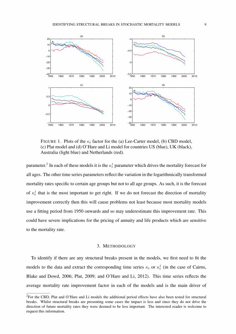
IDENTIFYING STRUCTURAL BREAKS IN STOCHASTIC MORTALITY MODELS 9
1950 1960 1970 1980 1990 2000 2010−40
−30
−20
−10
0
10
20(a)
1950 1960 1970 1980 1990 2000 2010−5.5
−5
−4.5
−4(b)
1950 1960 1970 1980 1990 2000 2010−1
−0.5
0
0.5
1(c)
1950 1960 1970 1980 1990 2000 2010−40
−30
−20
−10
0
10
20(d)
FIGURE 1. Plots of the κt factor for the (a) Lee-Carter model, (b) CBD model,(c) Plat model and (d) O’Hare and Li model for countries US (blue), UK (black),Australia (light blue) and Netherlands (red).
parameter.2 In each of these models it is the κ1t parameter which drives the mortality forecast for
all ages. The other time series parameters reflect the variation in the logarithmically transformed
mortality rates specific to certain age groups but not to all age groups. As such, it is the forecast
of κ1t that is the most important to get right. If we do not forecast the direction of mortality
improvement correctly then this will cause problems not least because most mortality models
use a fitting period from 1950 onwards and so may underestimate this improvement rate. This
could have severe implications for the pricing of annuity and life products which are sensitive
to the mortality rate.
3. METHODOLOGY
To identify if there are any structural breaks present in the models, we first need to fit the
models to the data and extract the corresponding time series κt or κ1t (in the case of Cairns,
Blake and Dowd, 2006; Plat, 2009; and O’Hare and Li, 2012). This time series reflects the
average mortality rate improvement factor in each of the models and is the main driver of
2For the CBD, Plat and O’Hare and Li models the additional period effects have also been tested for structuralbreaks. Whilst structural breaks are presenting some cases the impact is less and since they do not drive thedirection of future mortality rates they were deemed to be less important. The interested reader is welcome torequest this information.

10 O’HARE AND LI
the forecasts of mortality derived from each of the models. We use Box-Jenkins approach
to identify the most suitable ARIMA process to fit to the extracted κt which in all cases turns
out to be a simple random walk with drift. If the selected ARIMA processes are appropriate
then we should expect residuals whose mean does not deviate significantly from zero. We apply
a generalised fluctuations test and that of Bai and Perron (1998, 2003) to identify and date the
structural breaks present.
3.1. Cumulative sums of residuals. The generalised fluctuation test framework includes for-
mal significance tests. Essentially, the techniques are designed to bring out departures from
constancy in a graphic way instead of parameterizing particular types of departure in advance
and then developing formal significance tests intended to have high power against these par-
ticular alternatives. More precisely, the model is fitted to the data and an empirical process is
derived that captures the fluctuation either in residuals or in parameter estimates. Under the
null hypothesis these are governed by functional central limit theorems (see Kuan and Hornik,
1995) and therefore boundaries can be found that are crossed by the corresponding limiting pro-
cesses with fixed probability α under the null hypothesis. Under the alternative the fluctuation
in the process is in general increased. Also, the trajectory of the process often sheds light on
the type of deviation from the null hypothesis such as the dating of the structural breaks. There
are several types of fluctuation tests, we outline the test using a cumulative sum of residuals for
information.
The first type of empirical fluctuations process that can be computed are cumulative sums of
residuals processes (CUSUM), which contain cumulative sums of standardized residuals. These
can be calculated recursively or using ordinary least squares. Brown et al. (1975) suggested to
consider cumulative sums of recursive residuals:
(6) Wn(t) =1
σ√η
k+[tη ]∑i=k+1
ui,
where η = n−k is the number of recursive residuals and [tη] is the integer part of tη. Under this
approach the null hypothesis the limiting process for the empirical fluctuation process Wn(t)
is the standard Brownian motion W (t). More precisely the functional central limit theorem
holds: Wn ⇒ W as n→∞, where⇒ denotes weak convergence of the associated probability
measures. Under the alternative, if there is just a single structural change point t0, the recursive

IDENTIFYING STRUCTURAL BREAKS IN STOCHASTIC MORTALITY MODELS 11
residuals will only have zero mean up to t0. Hence the path of the process should be close to 0
up to t0 and leave its mean afterwards.
The alternative of using ordinary least squares proposed by Ploberger and Kramer (1992),
bases a structural change test on cumulative sums of the common OLS residuals. Thus, the
empirical fluctuation process is defined by:
(7) W 0n(t) =
1
σ√n
[nt]∑i=1
ui.
The limiting process for W 0n(t) is the standard Brownian bridge W 0(t) = W (t) − tW (1). It
starts in 0 at t = 0 and it also returns to 0 for t = 1. Under a single structural shift alternative the
path should have a peak around t0. As an alternative we can calculate moving sums of residuals
rather than cumulative. Again we may calculate the residuals recursively or using ordinary least
squares.
3.2. Bai and Perron’s method. The idea of Bai and Perron (1998, 2003) is to estimate break
points based on calculating the global minimisers of the sum of squared residuals from say, a
regression model. Consider the piecewise linear regression method to compute the global min-
imisers of the objective function. The piecewise linear function begins with an ordering of the
observations and applies a dynamic program. With a sample of size T , the total number of pos-
sible segments is at most T (T + 1)/2. The global sum of squared residuals for any m-partition
and for any value of m must necessarily be a particular linear combination of these T (T +1)/2
sums of squared residuals. The estimates of the break dates, the m-partition (T1, ..., Tm), corre-
spond to this linear combination which must have a minimal value of sum of squared residuals,
so that an optimal partition can be selected over all possible m-partitions. Once the sums of
squared residuals of the relevant partitions have been computed, a dynamic programming algo-
rithm can be used to compare possible combinations, and then find a partition which achieves a
global minimization over the entire sum of squared residuals. This method essentially proceeds
through a sequential examination of optimal one-break partitions. Based on a recursive pro-
cedure. It simply minimizes sum of squared residuals over the set of possibilities obtained by
assuming the first j elements have been optimally partitioned in m− 1+ 1 parts and that m+1
part consists of the last T − j + 1 elements. The optimal partitions can be obtained iteratively.

12 O’HARE AND LI
Bai and Perron’s method is mostly used in the literature in identifying structural breaks,
recently Zeileis et al. (2003) developed the R package strucchange which includes most of the
existing procedures dealing with structural breaks and their latest developments, for instance
Zeileis (2000, 2005).
4. EMPIRICAL ANALYSIS
In the following sections first we now formalise our tests for structural breaks in the time
series that we have extracted from each of the models in the previous section. To clarify, we
have fit each of the models to the Male mortality data of the US, UK, Netherlands and Australia
between the years 1950 - 2000 inclusive. We have then extracted the main mortality improve-
ment factor κt or κ1t from each of the models and fitted a random walk with drift process as the
Box-Jenkins identified best ARIMA process to fit the time series. If the random walk process
is indeed an appropriate time series capturing the κt or κ1t factor then the resulting residuals
should have a mean which does not deviate from zero. We test this using the empirical fluctu-
ations test framework described by Zeileis et al. (2003). Furthermore, we use the methods of
Bai and Perron (1998, 2003) to identify structural breaks. Then, we fit and forecast the models
with and without structural breaks.
4.1. Identifying structural breaks. The structural change is located and dated by plotting
the cumulative sum of residuals and then comparing this with the known limiting processes.
Fluctuations that fall outside these known boundaries are judged to be improbably large and
hence suggest a structural change in the mean value. The known limiting process, otherwise
known as the boundary is plotted along with the cumulative sum of residuals in figure 2 and
figures 8 to 10 in the appendix.
As can be seen from the above tests there are unexpectedly large fluctuations (demonstrating
the presence of a structural break) for the majority of cases considered. However, the results are
not as conclusive as in the cases of Li, Chan, and Cheung (2011) and Coelho and Nunes (2011).
For the Lee-Carter model there appears to be a structural break present for 3 out of the 4 coun-
tries considered with the only country for which the above test does not confirm the presence
of a structural break being the UK. In the case of the CBD model we have similar conclusions
with again the extracted mortality improvement factor κ1t , for the UK not demonstrating any
presence of a structural break under the test we have carried out. For the larger factor models

IDENTIFYING STRUCTURAL BREAKS IN STOCHASTIC MORTALITY MODELS 13
FIGURE 2. Cumulative sum of residuals test for the Lee-Carter model for (fromtop left clockwise) US, UK, Netherlands and Australia with boundaries shownin red
of Plat (2009) and O’Hare and Li (2012) the results are mixed again. In the case of Plat (2009),
the fluctuations test showed up a structural break for all four countries considered whilst the
O’Hare and Li (2012) model did not show up any structural breaks for the US or the UK. This
could be due to the quadratic effect parameter α1x applied to the κ1t in the case of the O’Hare
and Li (2012) model as compared with the linear α1t in the Plat (2009) case. In all the models
considered we were able to identify some structural breaks for some countries.
Having identified the presence of structural breaks the next step is to date these and then
using this information, re-forecast the models allowing for the structural break. We date the
structural break using Bai and Perron’s method. As can be seen from the table 3 and the figures
3 and figures 11 - 13 in the appendix the structural breaks identified occur with the period 1968
- 1979 with the vast majority occurring in the early 1970’s. This confirms previous findings and
would be well worth further investigation.

14 O’HARE AND LI
FIGURE 3. Test of the structural break for the Lee-Carter model for (from topleft clockwise) US, UK, Netherlands and Australia.
4.2. Empirical analysis of modelling with and without structural changes. Having identi-
fied and dated the presence of a structural break in each of the κt factors for our models we fit
each of the models again but this time allowing for the structural break. Again we fit up to the
year 2000 and forecast from 2001 to 2006 inclusive. We allow for the identified acceleration in
the mortality improvement factor κt by refitting the model using a data set in each case which
excludes data prior to the year in which the structural break occurs. Again we measure the fore-
casting quality using the average error (E1), the mean absolute error (E2) and the root mean
square error (E3). The results are outlined in table 4 with and without this adjustment.
As can be seen in table 4 in two-thirds of the cases allowing for the structural break results in
a more accurate forecast measured on any of the three measures considered. In the case of the
Netherlands, in every case allowing for the structural break improved the result. This indicates
that structural changes should be allowed for if we are to accurately forecast mortality rates.
The consequences of not allowing for structural breaks in the modelling process for mortality

IDENTIFYING STRUCTURAL BREAKS IN STOCHASTIC MORTALITY MODELS 15
TABLE 3. Break date results for UK, US, Netherlands and Australia using theLee-Carter, CBD, Plat, and O’Hare and Li models.
Model and Country Break date test statistic p-valueLee-CarterUK 1979 1.116 0.166US 1968 1.603 0.012Netherlands 1972 1.673 0.007Australia 1970 1.623 0.010CBDUK 1979 1.248 0.089US 1972 1.582 0.013Netherlands 1972 1.863 0.002Australia 1970 1.822 0.003PlatUK 1979 1.566 0.015US 1972 1.392 0.041Netherlands 1970 1.728 0.005Australia 1970 2.361 0.001O’Hare and LiUK 1979 1.366 0.048US 1972 1.288 0.072Netherlands 1972 1.648 0.009Australia 1970 2.126 0.001
rates are significant. In addition to the obvious issue of misspecifying the direction of the period
improvement factor there is also the issue of projecting confidence intervals which may be too
wide or too narrow depending on whether or not the break has been included in the fitting
period. Since the ideal fitting period cannot be known in advance further work is required to
ensure that appropriate caveats are included in any linear time series models.
We note that in allowing for the presence of structural breaks reduces the bias of the models,
see for example the CBD, Plat and O’Hare and Li models applied to US data where the E1
measure is improved by 3%-6%. This is to be expected since if we do not allow for structural
breaks then our linear trend will either overestimate or underestimate all rates beyond the break
date. We also note, looking at the E2 measure, that the absolute error is improved by as much
as 3% in the case of the Netherlands over a 5 year forecasting window. If we were to extrapolate
this forecast further into the future, as is very common when pricing mortality related products,
then this different in forecasting ability would become more pronounced.
We also plot the forecasted mortality rates with allowance (in green) and without allowance
(in blue) for the structural break. These can be seen in the case of the Lee Carter (1992) model
in figures 4 - 7. The figures for the Cairns, Blake and Dowd (2006), Plat (2009) and O’Hare

16 O’HARE AND LI
TABLE 4. Forecasting results for US, UK, Netherlands and Australia male mor-tality rates by single age 20-89, 2001-2006 measured on E1, E2 and E3 withand without allowance for structural breaks.
Structural break No Structural breakE1 E2 E3 E1 E2 E3
USLee-Carter 1.5% 7.3% 1.0% 2.8% 8.0% 1.2%CBD -6.2% 15.2% 5.3% -3.6% 16.4% 5.6%Plat -6.4% 9.0% 1.3% -3.6% 7.4% 0.8%O’Hare and Li -6.1% 8.5% 1.4% -0.1% 5.5% 0.5%UKLee-Carter 3.3% 9.0% 1.6% -1.7% 9.3% 1.2%CBD -4.8% 20.0% 7.5% 0.4% 24.0% 9.3%Plat 3.3% 9.5% 2.5% 3.3% 9.6% 2.2%O’Hare and Li 3.8% 12.0% 4.1% 7.6% 9.6% 2.1%NetherlandsLee-Carter 5.5% 9.4% 1.6% 7.4% 10.6% 2.0%CBD 0.8% 20.7% 7.5% 4.4% 22.7% 8.5%Plat 4.3% 9.3% 1.5% 5.4% 10.0% 1.7%O’Hare and Li 4.1% 10.1% 1.7% 11.1% 13.2% 3.0%AustraliaLee-Carter 4.6% 12.1% 3.2% 4.8% 11.5% 2.6%CBD -1.7% 28.7% 12.6% 2.3% 31.0% 14.0%Plat 6.6% 13.1% 6.7% 8.9% 13.2% 6.5%O’Hare and Li 11.8% 29.6% 28.6% 13.8% 16.3% 6.7%
and Li (2012) show similar patterns and are available upon request. The graphical figures show
us even more than the point estimates. In particular, we can see from these figures the direction
of the forecast with and without allowing for the structural break is very different leading to
very different predictions for future mortality rates. In the majority of cases allowing for the
structural break leads to lower mortality rates. This is particularly marked for the forecast
improvements for the older ages where the gap between forecasts is wider. For example see the
Lee-Carter forecasts in figure 7. The marked difference also seems to be greater for the UK and
Netherlands and less pronounced for the US.
We also note some of the results for the Carins, Blake and Dowd (2006) two factor model
which shows some bias problems at the lower ages. The model was designed for ages 60 and
above and so not surprisingly shows some unusual behaviour at the lower ages. It also forecasts
smoothly increasing mortality rates at the older ages, this is due to the fact that when the model
is fitted to the data the fitted mortality rates are smoother and lower than the actual mortality
rates. That being said the same issue of changing direction of forecast when allowing for the

IDENTIFYING STRUCTURAL BREAKS IN STOCHASTIC MORTALITY MODELS 17
structural break still persists with the CBD model as it does in the majority of these types of
models.
1950 1960 1970 1980 1990 2000 2010 2020 20300
0.5
1
1.5
2
2.5x 10
−3 (a)
1950 1960 1970 1980 1990 2000 2010 2020 20300.5
0.6
0.7
0.8
0.9
1
1.1
1.2
1.3
1.4
1.5x 10
−3 (b)
1950 1960 1970 1980 1990 2000 2010 2020 20300
0.2
0.4
0.6
0.8
1
1.2x 10
−3 (d)
1950 1960 1970 1980 1990 2000 2010 2020 20301
1.2
1.4
1.6
1.8
2
2.2x 10
−3 (c)
FIGURE 4. Forecasts of mortality rates for a 20 year old for the Lee-Cartermodel with allowance (in green) and without allowance (in blue) for the struc-tural break for (from top left clockwise) Australia, UK, US, and Netherlands.
1950 1960 1970 1980 1990 2000 2010 2020 20300.5
1
1.5
2
2.5
3
3.5x 10
−3 (a)
1950 1960 1970 1980 1990 2000 2010 2020 20300.5
1
1.5
2
2.5
3
3.5x 10
−3 (b)
1950 1960 1970 1980 1990 2000 2010 2020 20300.8
1
1.2
1.4
1.6
1.8
2
2.2
2.4
2.6x 10
−3 (d)
1950 1960 1970 1980 1990 2000 2010 2020 20301.5
2
2.5
3
3.5
4
4.5
5x 10
−3 (c)
FIGURE 5. Forecasts of mortality rates for a 40 year old for the Lee-Cartermodel with allowance (in green) and without allowance (in blue) for the struc-tural break for (from top left clockwise) Australia, UK, US, and Netherlands.

18 O’HARE AND LI
1950 1960 1970 1980 1990 2000 2010 2020 20300
0.005
0.01
0.015
0.02
0.025(a)
1950 1960 1970 1980 1990 2000 2010 2020 20300
0.005
0.01
0.015
0.02
0.025(b)
1950 1960 1970 1980 1990 2000 2010 2020 20300.005
0.01
0.015
0.02(d)
1950 1960 1970 1980 1990 2000 2010 2020 20300.005
0.01
0.015
0.02
0.025
0.03(c)
FIGURE 6. Forecasts of mortality rates for a 60 year old for the Lee-Cartermodel with allowance (in green) and without allowance (in blue) for the struc-tural break for (from top left clockwise) Australia, UK, US, and Netherlands.
1950 1960 1970 1980 1990 2000 2010 2020 20300.02
0.04
0.06
0.08
0.1
0.12
0.14(a)
1950 1960 1970 1980 1990 2000 2010 2020 20300.04
0.06
0.08
0.1
0.12
0.14
0.16(b)
1950 1960 1970 1980 1990 2000 2010 2020 20300.075
0.08
0.085
0.09
0.095
0.1
0.105
0.11
0.115(d)
1950 1960 1970 1980 1990 2000 2010 2020 20300.05
0.06
0.07
0.08
0.09
0.1
0.11
0.12(c)
FIGURE 7. Forecasts of mortality rates for a 80 year old for the Lee-Cartermodel with allowance (in green) and without allowance (in blue) for the struc-tural break for (from top left clockwise) Australia, UK, US, and Netherlands.
5. CONCLUSIONS
In this paper we have considered several of the leading extrapolative models of mortality rates
and have applied the methods of Bai and Perron (2003) to test for the presence of structural
breaks in the model specifications. More specifically we have fitted the models of Lee and
Carter (1992), Cairns, Blake and Dowd (2006), Plat (2009) and O’Hare and Li (2012) to the

IDENTIFYING STRUCTURAL BREAKS IN STOCHASTIC MORTALITY MODELS 19
data for US, UK, Australia and the Netherlands. Having noted that the forecasts of mortality
resulting from these models are driven primarily by the κt (or κ1t ) parameter, we have fitted the
best ARIMA process to the extracted time series and then tested the residuals for deviation from
zero. In fitting the ARIMA model to the κt period effect we are following the methods used by
Lee and Carter (1992) and others.
In each case we found that there was indeed a breakpoint visible in the residuals falling some-
where around the 1970’s confirming previous demographic research. We have not considered
the cause of the structural break or indeed whether the test is picking up a genuine structural
break or a gradual change in the improvement in mortality rates. In either case we have identi-
fied a pattern in the data that the ARIMA modelling approach does not capture. Identifying the
breaks, we then carried out the forecasting process again making allowance for the structural
break. The results show that in nearly two-thirds of cases the model allowing for structural
breaks provides a more accurate forecast measured on each of the E1, E2, and E3 measures.
Further research will widen the study to consider more countries and both male and female
populations to see if the results can be reported more widely.
The findings are significant in highlighting the importance of the sample period when fit-
ting a model to mortality data; however, they make no reference to possible future structural
breaks. Further research could look at more recent developments in the identification of struc-
tural breaks in models. Namely, monitoring data for structural breaks as and when they occur,
this would then allow for these breaks to be incorporated into mortality models more efficiently
reducing any future forecast errors.

20 O’HARE AND LI
Appendix: Additional Figures and Tables
FIGURE 8. Cumulative sum of residuals test for the CBD model for (from topleft clockwise) US, UK, Netherlands and Australia with boundaries shown inred.

IDENTIFYING STRUCTURAL BREAKS IN STOCHASTIC MORTALITY MODELS 21
FIGURE 9. Cumulative sum of residuals test for the Plat model for (from topleft clockwise) US, UK, Netherlands and Australia with boundaries shown inred.

22 O’HARE AND LI
FIGURE 10. Cumulative sum of residuals test for the O’Hare and Li model for(from top left clockwise) US, UK, Netherlands and Australia with boundariesshown in red.

IDENTIFYING STRUCTURAL BREAKS IN STOCHASTIC MORTALITY MODELS 23
FIGURE 11. Test of the structural break for the CBD model for (from top leftclockwise) US, UK, Netherlands and Australia.

24 O’HARE AND LI
FIGURE 12. Test of the structural break for the Plat model for (from top leftclockwise) US, UK, Netherlands and Australia.

IDENTIFYING STRUCTURAL BREAKS IN STOCHASTIC MORTALITY MODELS 25
FIGURE 13. Test of the structural break for the O’Hare and Li model for (fromtop left clockwise) US, UK, Netherlands and Australia.

26 O’HARE AND LI
REFERENCES
[1] Bai, J., and Perron, P. (1998), Estimating and Testing Linear Models With Multiple Structural Changes,
Econometrica, 66, 47-78.
[2] Bai, J., and Perron, P. (2003), Computation and Analysis of Multiple Structural Change Models, Journal of
Applied Econometrics, 18, 1-22.
[3] Booth, H., Maindonald, J., and Smith, L. (2002), Applying Lee-Carter under conditions of variable mortality
decline.Population Studies 56, 325-336.
[4] Booth, H., and Tickle, L. (2008), Mortality modeling and forecasting: A review of methods, Annals of
actuarial science. 3, 3-43.
[5] Brouhns, N., Denuit, M., and Vermunt, J.K. (2002), A Poisson log-bilinear approach to the construction of
projected lifetables. Insurance: Mathematics and Economics 31(3), 373-393.
[6] Brown R.L., Durbin J., Evans J.M. (1975), Techniques for testing constancy of regression relationships over
time, Journal of the Royal Statistical Society, Series B, 37, 149-163.
[7] Cairns, A.J.G., Blake, D., and Dowd, K. (2006), A two-factor model for stochastic mortality with parameter
uncertainty: Theory and calibration. Journal of Risk and Insurance 73, 687-718.
[8] Cairns, A.J.G., Blake, D., Dowd, K., Coughlan, G.D., Epstein, D., Ong, A., and Balevich, I. (2009), A
quantitative comparison of stochastic mortality models using data from England & Wales and the United
States. North American Actuarial Journal 13(1), 1-35.
[9] Cairns, A.J.G., Blake, D., Dowd, K., Coughlan, G.D., Epstein, D., and Khalaf-Allah, M. (2011), Mortality
density forecasts: An analysis of six stochastic mortality models.Insurance: Mathematics and Economics 48,
355-367.
[10] Carter, L. R., and Prskawetz., A. (2001), Examining Structural Shifts in Mortality Using the Lee-Carter
Method. Working Paper WP 2001-007, Max Planck Institute for Demographic Research
[11] Chu, C.S., Hornik, K., Kuan, C.M. (1995), MOSUM tests for parameter constancy, Biometrika, 82, 603-617.
[12] Clayton, D. and Schifflers, E. (1987), Models for temporal variation in cancer rates. II: Age-period-cohort
models. Statistics in Medicine, 6, 469-481.
[13] Coelho, E. and Nunes, L. C. (2011), Forecasting mortality in the event of a structural change. Journal of the
Royal Statistical Society: Series A (Statistics in Society), 174, 713-736.
[14] Currie, I.D. (2006), Smoothing and forecasting mortality rates with P-splines.Presentation to the Institute of
Actuaries. Available at: http://www.ma.hw.ac.uk/ iain/research.talks.html.
[15] Currie, I.D. (2011), Modelling and forecasting the mortality of the very old. ASTIN Bulletin, 41, 419-427.
[16] Delwarde, A., Denuit, M., and Eilers, P. (2007), Smoothing the Lee-Carter and Poisson log-bilinear models
for mortality forecasting: A penalized log-likelihood approach. Statistical Modelling, 7, 29-48.
[17] De Jong, P., and Tickle, L. (2006), Extending the Lee-Carter model of mortality projection. Mathematical
Population Studies, 13, 1-18.

Bibliography 27
[18] Girosi, F., and King, G. (2005), A reassessment of the Lee-Carter mortality forecasting method, Working
Paper, Harvard University.
[19] Harris, D., Harvey, D. I., Leybourne, S. J. and Taylor, A. M. R. (2009), Testing for a unit-root in the presence
of a possible break in trend. Econmetric Theory, 25, 1545-1588.
[20] Harvey, D. I., Leybourne, S. J. and Taylor, A. M. R. (2009), Simple, robust and powerful tests of the changing
trend hypothesis. Econmetric Theory, 25, 995-1029.
[21] Kannisto, V., Lauristen, J., Thatcher, A.R., and Vaupel. J.W. (1994), Reduction in Mortality at Advanced
Ages: Several Decades of Evidence from 27 Countries. Population Development Review, 20, 793-810.
[22] Koissi, M.C., Shapiro, A.F., and Hognas, G. (2005), Evaluating and Extending the Lee-Carter Model for
Mortality Forecasting: Bootstrap Confidence Interval. Insurance: Mathematics and Economics, 38, 1-20.
[23] Kuan, C.M., and Hornik, K. (1995), The generalized fluctuation test: A unifying view, Econometric Reviews,
14, 135-161.
[24] Lee, R.D., and Carter, L.R. (1992), Modeling and Forecasting U. S. Mortality, Journal of the American
Statistical Association, 87(419), 659-671.
[25] Lee, R. D., and Miller, T. (2001), Evaluating the performance of the Lee-Carter method for forecasting
mortality, Demography, 38, 537-549.
[26] Li, J.S.H., Chan, W.S., and Cheung, S.H. (2011), Structural Changes in the Lee-Carter Mortality Indexes:
Detection and Implications, North American Actuarial Journal, 15, 13-31.
[27] O’Hare, C., and Li, Y. (2012), Explaining young mortality, Insurance: Mathematics and Economics, 50(1),
12-25.
[28] Plat, R. (2009), On stochastic mortality Modeling. Insurance: Mathematics and Economics, 45(3), 393-404.
[29] Ploberger, W., and Kramer, W. (1992), The CUSUM test with OLS residuals, Econometrica, 60, 271-285.
[30] Renshaw, A.E., and Haberman, S. (2003), Lee-Carter mortality forecasting with age-specific enhance-
ment.Insurance: Mathematics and Economics, 33, 255-272.
[31] Renshaw, A.E., and Haberman, S. (2006), A cohort-based extension to the Lee-Carter model for mortality
reduction factors. Insurance: Mathematics and Economics, 38, 556-70.
[32] Tuljapurkar, S., and Boe, C. (1998), Mortality Change and Forecasting: How Much and How Little Do We
Know? North American Actuarial Journal, 2, 13-47.
[33] Vaupel, J.W. (1997), The Remarkable Improvements in Survival at Older Ages. Philosophical Transactions
of the Royal Society of London, B 352, 1799-1804.
[34] Zeileis, A. (2000), p-values and alternative boundaries for CUSUM tests. Working Paper 78, SFB Adaptive
Information Systems and Modelling in Economics and Management Science, http://www.wu-wien.
ac.at/am/wp00.htm#78.
[35] Zeileis, A., Kleiber C., Kramer W., and Hornik K. (2003), Testing and Dating of Structural Changes in
Practice, Computational Statistics and Data Analysis, 44, 109-123.

28 Bibliography
[36] Zeileis, A. (2005), A Unified Approach to Structural Change Tests Based on ML Scores, F Statistics and OLS
Residuals. Econometric Reviews, 24, 445-466.
[37] Zivot, E., and Andrews, D. (1992), Further Evidence of the Great Crash, the Oil-Price Shock and the Unit-
Root Hypothesis. Journal of Business and Economic Statistics, 10, 251-270.
![Advances in Stochastic Mortality Modelling[Toczydlowska and Peters, 2017]considered stochastic projection methods of dimensionality reduction)Probabilistic Principal Component Analysis](https://static.fdocuments.us/doc/165x107/61207bccc7108002d73aba5b/advances-in-stochastic-mortality-modelling-toczydlowska-and-peters-2017considered.jpg)


