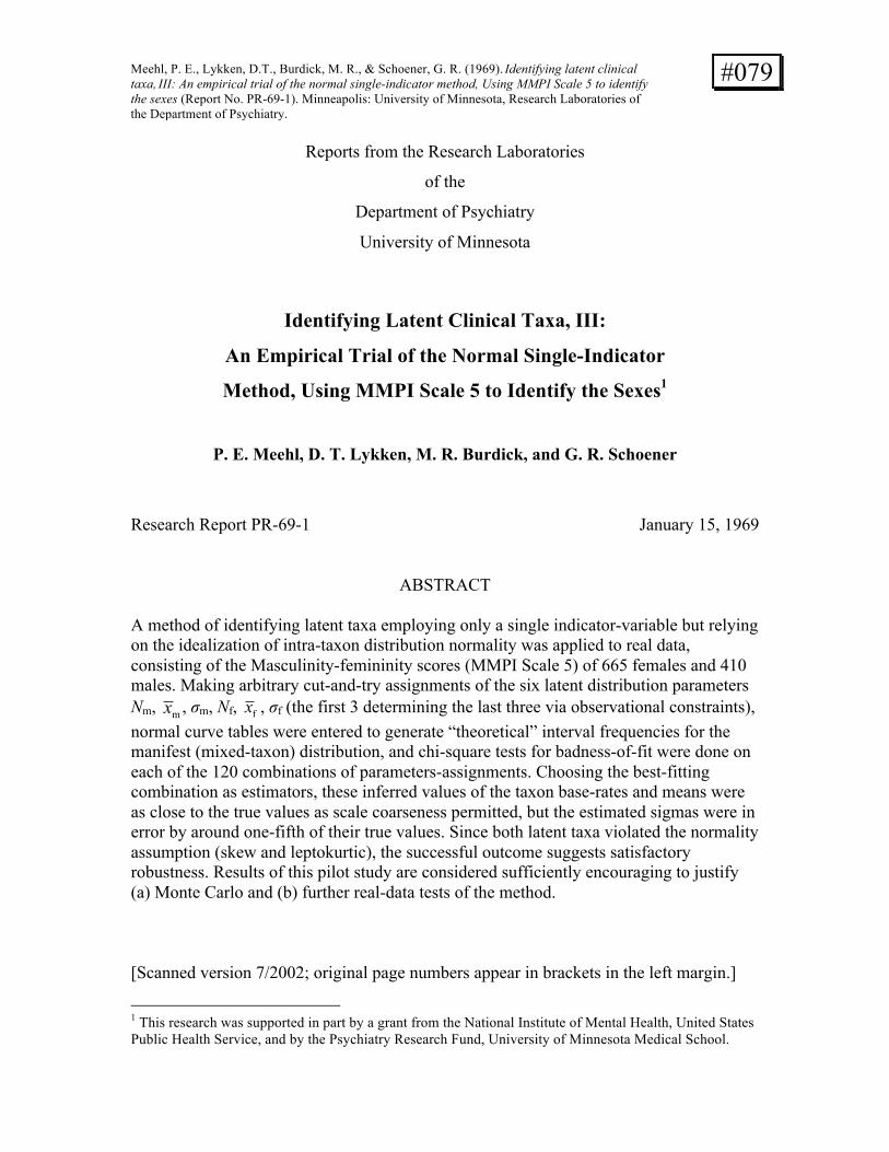
Meehl, P. E., Lykken, D.T., Burdick, M. R., & Schoener, G. R. (1969). Identifying latent clinical taxa, III: An empirical trial of the normal single-indicator method, Using MMPI Scale 5 to identify the sexes (Report No. PR-69-1). Minneapolis: University of Minnesota, Research Laboratories of the Department of Psychiatry.

#079

Reports from the Research Laboratories

of the

Department of Psychiatry

University of Minnesota

Identifying Latent Clinical Taxa, III:

An Empirical Trial of the Normal Single-Indicator

Method, Using MMPI Scale 5 to Identify the Sexes1

P. E. Meehl, D. T. Lykken, M. R. Burdick, and G. R. Schoener

Research Report PR-69-1 January 15, 1969

ABSTRACT A method of identifying latent taxa employing only a single indicator-variable but relying on the idealization of intra-taxon distribution normality was applied to real data, consisting of the Masculinity-femininity scores (MMPI Scale 5) of 665 females and 410 males. Making arbitrary cut-and-try assignments of the six latent distribution parameters Nm, mx , σm, Nf, fx , σf (the first 3 determining the last three via observational constraints), normal curve tables were entered to generate “theoretical” interval frequencies for the manifest (mixed-taxon) distribution, and chi-square tests for badness-of-fit were done on each of the 120 combinations of parameters-assignments. Choosing the best-fitting combination as estimators, these inferred values of the taxon base-rates and means were as close to the true values as scale coarseness permitted, but the estimated sigmas were in error by around one-fifth of their true values. Since both latent taxa violated the normality assumption (skew and leptokurtic), the successful outcome suggests satisfactory robustness. Results of this pilot study are considered sufficiently encouraging to justify (a) Monte Carlo and (b) further real-data tests of the method. [Scanned version 7/2002; original page numbers appear in brackets in the left margin.]

1 This research was supported in part by a grant from the National Institute of Mental Health, United States Public Health Service, and by the Psychiatry Research Fund, University of Minnesota Medical School.

[1] In a previous contribution to this Research Report series (Meehl, 1968, Section 3,

pages 47-54) a method was proposed for identifying the presence of a latent taxonomic

situation (dichotomous case) when only a single fallible indicator-variable is available, as

contrasted with the (much preferable) situation in which a family of three or more

construct-valid indicators are known to discriminate, which was the psychometric

situation mainly emphasized in previous contributions (Meehl, 1965, 1968; but see also

Dawes & Meehl, 1966). The mathematical rationale will not be repeated here, for which

the reader is referred to the earlier report at the cited locus. Suffice it to say here that

whereas the multiple-indicator methods make only weak assumptions about the

distribution shapes for single indicators of the indicator-family, the present one-indicator

technique relies upon an approximative assumption of intra-taxon normality, i.e., we

assume that within each of the two latent taxa being sought for, the indicator in use is,

while not precisely normal, sufficiently close to normal that the method can be used

without gross distortion of the underlying reality.

The reader is referred to equations [99]–[103] of PR-68-4 (page 51 of Meehl, 1968)

[2] which set up the simple algebra of the situation. One first assigns arbitrary base-

frequency for one of the taxa. This determines the base-frequency for the other taxon.

Holding these values fixed, one assigns an arbitrary mean to one of the taxa, which

assignment, given the base-frequency values presupposed in the preceding step,

determines the mean of the other taxon. Finally one assigns an arbitrary standard

deviation to one of the taxa, which assignment, given the preceding assignments (and

implied values) of the frequencies and means, determines the standard deviation of the

other taxon. So that the arbitrary assignment of a base-frequency, a mean, and a sigma to

one taxon determines the corresponding values for the other taxon. These consequences

are algebraic identities and do not depend upon the normality assumptions. However, to

generate an expected manifest-distribution frequency from any of the various

combinations of latent assignments that thus arise, some assumption regarding

distribution form must be made. If we make the normality assumption within taxa, each

triad of arbitrary values (Ns, sx , σs) determines expected frequencies in class-intervals of

the latent frequency function for the first postulated taxon; and in the same way the other

taxon’s parameter values (Nn, nx , σn) that are determined algebraically by the first

taxon’s parameter values will generate as set of expected frequencies for each class

interval of the latent frequency function for the second taxon. When these two latent

frequency functions, flowing necessarily from the arbitrary parameter assignments

(together with the normality postulate) are superimposed, we thereby generate an

[3] expected distribution of manifest frequencies (mixed taxa). That set of theoretically

calculated frequencies is then compared with the observed, the discrepancy measured by

chi-square as usual, and the chi-square value recorded as one point on a curve of theory-

observation discrepancies. The entire process is then repeated, first for differing values of

sigma (holding the frequencies and means fixed), then for the same range of values of

sigma (holding fixed a different pair of means and taxon-rates); and, finally, running

through the same set of sigmas and the same set of means but with another arbitrary set

of frequencies. We thus generate a family of curve-families of chi-squares representing

observation-theory discrepancies, and we assume that the minimum chi-square —

hopefully a statistically nonsignificant one — corresponds to the underlying latent taxon

situation.

Pending a large-scale Monte Carlo investigation of the sampling characteristics of

the method, it was thought worthwhile to try it out on some real data in which we would

pretend not to know which patients belonged to each latent taxon, what the latent means

and sigmas were, or even what the relative proportions of the two latent taxa were, to see

whether the method would give us anything like the right answers. It is not easy to locate

a true taxonomy in the area of psychometrics, but one of the good ones, both because it

does yield a genuine bimodality in personality scores and because it is completely

objective on the criterion side, is biological sex. We therefore applied the method to the

pseudo-problem of identifying the male-female taxonomy, using the MMPI masculinity-

[4] femininity scale as our single indicator-variable (Scale 5). The raw data were

computer print-outs of the Mf scores of 410 males and 665 females which had previously

been drawn randomly for another purpose from the University of Minnesota Hospital

“General Psychiatric Population.” The statistical characteristics of this pair of latent taxa

on MMPI Scale 5 are shown in Table 1.

Table 1

The Values of the Sample Statistics for Each Taxon

N Base-Rates x S.D.

Males 410 P = .38 24.73 5.75

Females 665 Q = .62 36.04 5.66

Total 1075 1.00 31.72 7.92

For this pilot study it was thought sufficient to try postulated frequencies for the

male taxon ranging from 100 (base rate P = .09) to 500 (base rate P = .46) proceeding by

100-case increments; that is, the hypothesized male frequencies tried against observation

were 100, 200, 300, 400, and 500, corresponding to hypothesized male base-rates of .09,

.19, .28, .37, and .46 respectively.

Given the observed grand (mixed taxon) mean of tx = 31.73, and the observed

grand (mixed taxon) standard deviation of 7.92, “safe” or “plausible” values of the

hypothesized latent mean for the males were considered to run from around 15 (raw

score) on MMPI Scale 5 to around double that value at mx = 30, and the variation in cut-

[5] and-try mean values for the males was run by five-unit steps; that is, we tried out

latent taxon mean of the males at the four values mx = 15, mx = 20, mx = 25, and mx = 30.

Given the grand observed (mixed-taxon) sigma of 7.92, arbitrary cut-and-try values

of the male taxon standard deviation were run from a low of 3 and proceeding by unit

steps of 4, 5, 6, and 7 through 8.

From this logical tree of arbitrary values assigned to each of the three latent

parameters, there follow, on the intra-taxon normality assumption, a set of 120

combinations (i.e., 5 arbitrary base rates x 4 arbitrary means x 6 arbitrary sigmas). This

would mean a comparison of the observed (mixed-taxon) frequency distributions with

each of the 120 cut-and-try distributions and the plotting of 120 chi-squares to identify

the best fit. Actually not all of these chi-squares, and not even all of the curves within a

curve-family, had to be computed and plotted, because some of the arbitrary parameter

assignments generated negative variances for the second [actually female] taxon. The

appearance of these negative variances caused us (foolishly) to double check for possible

computational error. There was no need to assume error on the usual grounds of the

algebraic impossibility of a negative variance when a sum of squares of deviations from a

mean is directly computed. When a variance is estimated by a combination of an

observed dispersion and an arbitrary latent taxon value, as in the present procedure, a

negative estimated variance can easily arise from sufficiently extreme [i.e., grossly

erroneous] arbitrary assignments of the variance (together with the base-rate and mean of

[6] one taxon). The correct inference from the appearance of a negative variance is, of

course, simply that these particular latent values are precluded by our empirical data,

which is what we are investigating!

In calculating the observational distribution from the postulated latent values, from

35 to 52 intervals of unit width (integer increments) on the Mf (raw score) variable were

employed, avoiding grouping coarseness problems. This amounts to intervals of width

approximately .13 sigma on the manifest distribution, and approximately .18 sigma on

each of the two latent taxon distributions. Calculated latent frequencies within a class

interval were rounded off to the nearest integer, combining intervals at tails whenever the

expected values were less than one (Cochran, 1954).

In Table 2 are shown the chi-square values and chi-square normal deviates

indicating the discrepancy between the observed grand (mixed-taxon) distribution and the

120 theoretically calculated distributions generated by the various sets of arbitrary latent

parameter values for the base-rates, means, and sigmas. Note that the lowest arbitrary

mean value tried for males ( mx = 15) gives rise to impossibly negative estimated

variances for the other latent taxon at 4 of the 5 arbitrary base-rates.

The raw Mf scores on the manifest (mixed-taxon) frequency distribution ran from

raw score = 9 through raw score = 49 inclusive (corresponding to T-scores from 106 to

28 for males, and from 24 to 95 for females, respectively), requiring a total of 41

ungrouped class-intervals to cover the empirically observed range.

[7]

Table 2

The Chi-square Values and Chi-square normal deviates

for Each of the 120 sets of Arbitrary Latent Values

Nm = 100

mx σm Intervals

Range Number Degrees of

Freedom (n) χ2 22 2 1nχ − − p

15 3 8 – 51 44 41 172 9.55 <.01

4 6 – 51 45 42 157 8.61 <.01

5 4 – 51 48 45 152 8.01 <.01

6 2 – 51 50 47 155 7.97 <.01

7 0 – 51 52 49 169 8.53 <.01

8 0 – 50 51 48 224 11.42 <.01

20 3 11 – 54 44 41 80 3.32 <.01

4 10 – 54 45 42 73 2.97 <.01

5 8 – 54 47 44 72 2.67 <.01

6 7 – 54 48 45 76 2.90 <.01

7 5 – 54 50 47 85 3.40 <.01

8 4 – 52 49 46 96 4.32 <.01

25 3 10 – 54 45 42 140 7.62 <.01

4 10 – 54 45 42 130 7.01 <.01

5 10 – 54 45 42 117 6.19 <.01

6 10 – 54 45 42 105 5.38 <.01

7 10 – 54 45 42 100 5.03 <.01

8 9 – 54 46 43 96 4.64 <.01

30 3 8 – 56 49 46 138 7.07 <.01

4 8 – 56 49 46 125 6.27 <.01

5 8 – 56 49 46 113 5.49 <.01

6 8 – 56 49 46 107 5.09 <.01

7 10 – 54 45 42 107 5.52 <.01

8 10 – 54 45 42 98 4.89 <.01

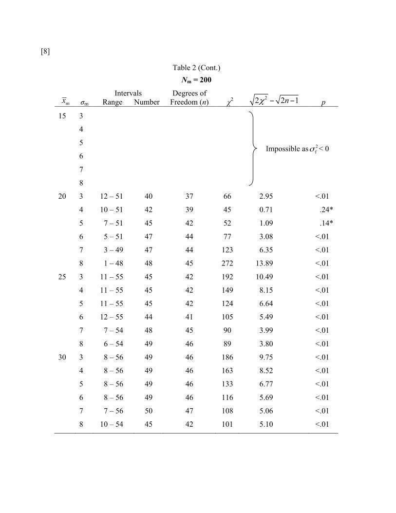
[8]

Table 2 (Cont.) Nm = 200

mx σm Intervals

Range Number Degrees of

Freedom (n) χ2 22 2 1nχ − − p

15 3

Impossible as 2fσ < 0

4

5

6

7

8

20 3 12 – 51 40 37 66 2.95 <.01

4 10 – 51 42 39 45 0.71 .24*

5 7 – 51 45 42 52 1.09 .14*

6 5 – 51 47 44 77 3.08 <.01

7 3 – 49 47 44 123 6.35 <.01

8 1 – 48 48 45 272 13.89 <.01

25 3 11 – 55 45 42 192 10.49 <.01

4 11 – 55 45 42 149 8.15 <.01

5 11 – 55 45 42 124 6.64 <.01

6 12 – 55 44 41 105 5.49 <.01

7 7 – 54 48 45 90 3.99 <.01

8 6 – 54 49 46 89 3.80 <.01

30 3 8 – 56 49 46 186 9.75 <.01

4 8 – 56 49 46 163 8.52 <.01

5 8 – 56 49 46 133 6.77 <.01

6 8 – 56 49 46 116 5.69 <.01

7 7 – 56 50 47 108 5.06 <.01

8 10 – 54 45 42 101 5.10 <.01

[9]

Table 2 (Cont.) Nm = 300

mx σm Intervals

Range Number Degrees of

Freedom (n) χ2 22 2 1nχ − − p

15 3

Impossible as 2fσ < 0

4

5

6

7

8

20 3 11 – 45 35 32 1053 37.9 <.01

4 9 – 43 35 32 1217 41.4 <.01

5 7 – 42 36 33 2045 56.0 <.01

6

Impossible as 2fσ < 0 7

8

25 3 12 – 56 44 41 280 14.70 <.01

4 12 – 56 44 41 188 10.40 <.01

5 11 – 55 44 41 131 7.19 <.01

6 9 – 55 46 43 104 5.20 <.01

7 7 – 53 47 44 76 3.00 <.01

8 5 – 52 48 45 70 2.40 <.01

30 3 6 – 58 53 50 267 13.20 <.01

4 6 – 58 53 50 203 10.20 <.01

5 8 – 56 49 46 163 8.52 <.01

6 8 – 56 49 46 136 6.85 <.01

7 8 – 56 49 46 108 5.16 <.01

8 10 – 54 45 42 102 5.17 <.01

[10]

Table 2 (Cont.) Nm = 400

mx σm Intervals

Range Number Degrees of

Freedom (n) χ2 22 2 1nχ − − p

15 3

Impossible as 2fσ < 0

4

5

6

7

8

20 3

4

5

6

7

8

25 3 16 – 56 41 38 318 16.60 <.01

4 14 – 55 42 39 196 11.00 <.01 Closestto TrueValue

⎫⎪⎬⎪⎭

5 11 – 55 45 42 118 6.25 <.01

6 9 – 53 45 42 72 2.89 <.01

7 6 – 51 46 43 40 –.28 .61**

8 4 – 48 45 42 70 2.72 <.01

30 3 5 – 61 57 54 380 17.42 <.01

4 7 – 59 53 50 268 13.65 <.01

5 7 – 59 53 50 198 9.95 <.01

6 9 – 57 49 46 152 7.90 <.01

7 8 – 57 50 47 112 5.34 <.01

8 9 – 55 47 44 99 4.74 <.01

**Best fit in 120 trial values

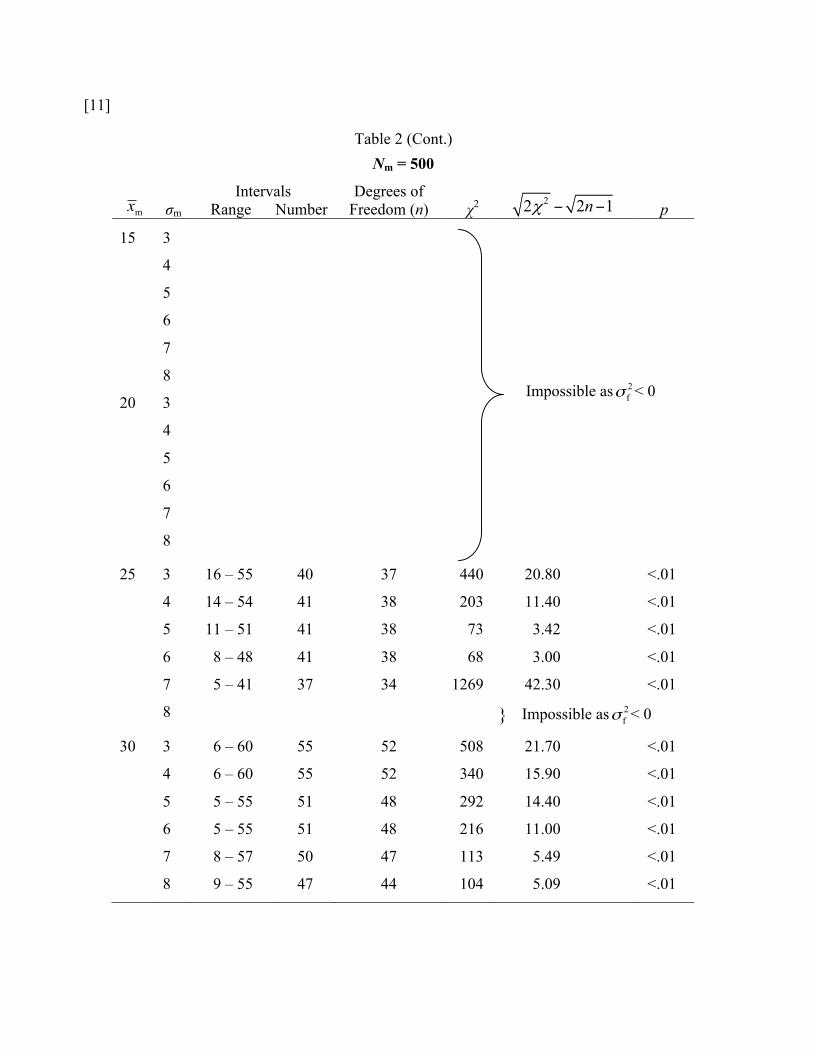
[11]

Table 2 (Cont.) Nm = 500

mx σm Intervals

Range Number Degrees of

Freedom (n) χ2 22 2 1nχ − − p

15 3

Impossible as 2fσ < 0

4

5

6

7

8

20 3

4

5

6

7

8

25 3 16 – 55 40 37 440 20.80 <.01

4 14 – 54 41 38 203 11.40 <.01

5 11 – 51 41 38 73 3.42 <.01 6 8 – 48 41 38 68 3.00 <.01

7 5 – 41 37 34 1269 42.30 <.01

8 } Impossible as 2fσ < 0

30 3 6 – 60 55 52 508 21.70 <.01

4 6 – 60 55 52 340 15.90 <.01

5 5 – 55 51 48 292 14.40 <.01

6 5 – 55 51 48 216 11.00 <.01

7 8 – 57 50 47 113 5.49 <.01

8 9 – 55 47 44 104 5.09 <.01

[12] The arbitrary parameter assignment method of course gives rise to non-zero “theoretical”

values for class-intervals outside the empirical range of scores, and in other cases predicts

near-zero frequencies for intervals that are actually occupied. Hence many of the chi-

squares are based upon more than the 38 [= 41 – 3] degrees of freedom that would be

involved in testing significance with 41 class intervals, and some are based on fewer d.f.

than this. Consequently the degrees of freedom varied considerably from one goodness-

of-fit test to another, rendering the obtained chi-square values not directly comparable

without taking the varying degrees of freedom into account. Although we plotted and

inspected the graphs of the raw chi-square values themselves, what is of proper interest

for purposes of estimating the true values of the best-fitting hexad of arbitrary parameters

is the function ( )22 2 1nχ − − treatable as a normal deviate with unit variance for d.f.

> 30. Table 2 shows the interval ranges, number of intervals, degrees of freedom, chi-

square value, the associated value of the chi-square deviate 22 2 1nχ − − , and the P-

value from normal curve tables. In the case of chi-square, of course, the proper P-value to

use is the integral under the normal function from the given chi-square deviate upward,

since probabilities associated with negative values of the normal chi-square deviate (as in

the best-fitting combination Nm = 400, mx = 25, σm = 7, where the deviate is at z = –.28)

are greater than ½, i.e., this assignment of parameters fits the empirical distribution better

[13] than one might expect on the average to fit it through random sampling fluctuations

alone.

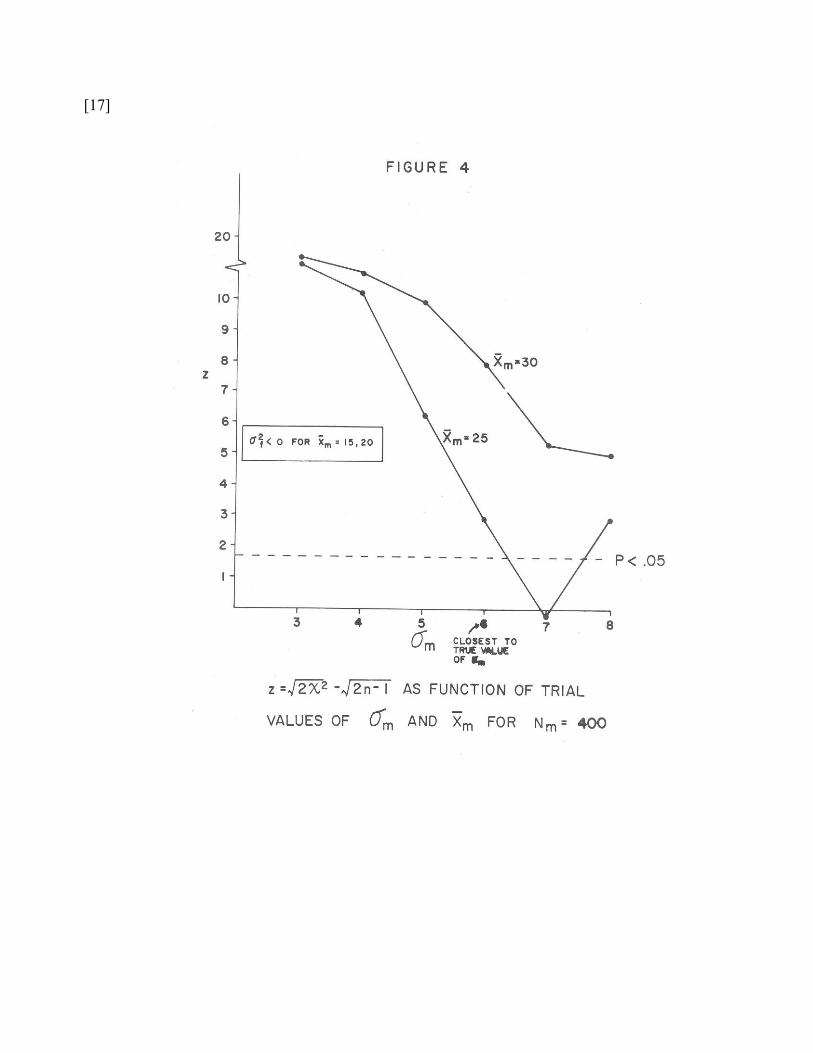
The chi-square deviate values in Table 2 are plotted as curve-families in Figures 1

through 5. Each figure represents a family of curves associated with one of the five

arbitrary assignments of the base-rate Nm. Each curve within the family represented by a

given figure shows the dependency of the chi-square deviate upon sigma assignment,

given a fixed assignment of the latent mean mx . And each plotted point on a given curve

within a family represents the chi-square deviate value obtained for an abscissa value of

the indicated sigma, given the arbitrary mean generating the curve on which the point is

found, and the arbitrary base-rate generating the family of curves represented in the

figure. So each point on one of these graphs indicates a chi-square deviate, corrected for

the variable degrees of freedom on which it was based, and reflecting the theoretical-

observed discrepancies yielded by the particular arbitrary parameter combination which

gave rise to it. As the curves rise, they reflect increasingly unsatisfactory parametric

assumptions about the latent situation. Thus, in Figure 1 the top curve shows the set of 6

chi-square deviates generated by arbitrary assignments of σ = 3, 4, …8 to the one latent

taxon, when the arbitrary mean assigned to that taxon is 15, given the fixed arbitrary

base-rate for that taxon arbitrarily assigned at Nm = 100. The four curves in Figure 1 show

the dependence of the goodness-of-fit upon the six arbitrary standard deviation

assignments, for each of the four

[14]

[15]

[16]

[17]

[18]

[19] arbitrary mean assignments, holding fixed an arbitrary base-rate assignment of 100. The

other four figures are to be interpreted the same way.

Before considering the question of how well the minimum of minima of minima

among all these curves succeeds in spotting the true latent values, certain general

observations on the way the curve families behave are of some interest. The figure whose

hypothetical base-rate is closest to the true one is of course Figure 4, with the first

[= male] taxon being arbitrarily assigned a base rate of Nm = 400, which with 100-unit

steps is as close as we can come to the true value of the number of males in this sample

(Nm = 410). We note that this graph, and the graph based upon the next closest available

base-rate assignment (Nm = 500, Figure 5) both exhibit a considerably greater “steepness”

or “peakedness” than is true of the curves in Figures 1, 2, and 3. The “flattest” curves, in

which the variation in arbitrary assignments of sigma values seems to make the least

difference in the goodness-of-fit to the observed data, we see in the most far-out

erroneous base rate value, at Nm = 100. Quaere, whether it is for some reason a general

principle in this procedure, that a “good” estimate of base-rate is necessary in order for

good-to-bad variations of the within-taxon parameter guesses to generate appreciable

variation in goodness-of-fit to the observations.

In Figure 2, where the lowest arbitrary mean assignment ( mx = 15) is not plottable

because it results in an impossible negative variance for the female taxon, there seems to

[20] be something aberrated about the curve reflecting the first algebraically possible value of

the arbitrary mean of mx = 20, in the sense that this curve cuts diametrically across the

other two instead of running roughly parallel to them, as the curves in the other figures

do.

The smallest chi-square deviate obtained (lowest empirical “badness-of-fit” point

on any curve in any curve-family) is found in Figure 4, which corresponds to a postulated

latent (male) taxon frequency of 400 (base-rate .37), the true value being 410 (base-rate

.38); a postulated latent mean of mx = 25, the true value being 24.73; and an assigned

latent sigma of 7 (the true value being σm = 5.75). So we do identify the correct curve-

family, and the correct curve within the family, the estimated values being very close to

the true ones; but we make an error of more than one raw-score unit in estimating the

latent sigma, not attributable to scale coarseness, since the nearest rounded-off integral

value to the true male sigma should be at 6 on the abscissa, instead of at 7. It does not

seem possible to say, upon contemplating this series of five figures, to what extent the

error in sigma-assignment is attributable to the coarseness of the discontinuous intervals

or to the fact that the intrataxon normality assumption is an idealization.

Fisher’s g-statistics were calculated on the latent distributions of males and females,

and (as was expected from previous work on the Mf scale) each of them differed

significantly from normal curve form (p < .001, as to both skewness and kurtosis, and for

both sexes). The male frequency function was considerably skewed to the right, the

female to the left, and both curves were quite markedly leptokurtic. The accurate estimate

[21] of base-rates and latent means, in spite of these sizeable departures from the normal-

curve idealization, speaks encouragingly for the method’s robustness.

It would be gratifying to find that the true or truest parameter assignments yielded a

nonsignificant p-value for chi-square and all others a significant one, but this is not the

case. One-tailed probability p < .05 (obviously “super-fit” chi-squares are of no interest

here) corresponds to a deviate z = 1.65, the dotted reference line shown in each figure,

and parameter estimates providing a “satisfactory fit” (p < .05, z < 1.65) occur three times

(in 120 trials) as seen in Figures 2 and 4. The arbitrary values yielding these good fits are

indicated by an asterisk in Table 2. Note that the only assignment yielding a fit “better

than chance expectation” — slightly below the expected chi-square deviate — is the σm =

7 value in Figure 4, i.e., the closest possible assignment of Nm and mx to the true values.

This is gratifying, but it must be admitted that the (badly-off) assignments in Figure 2 are

uncomfortably “good”-looking and do not reach the 5% level either.

With steps of this coarseness, an investigator starting “blind” in search of the latent

taxa, relying on a single indicator, and with no antecedent information as to the true base-

rates, means, or sigmas, would in this study have concluded that the one taxon had a

base-rate of approximately 400, a mean of approximately 25, and a standard deviation of

approximately 7. But while this is the best value, he would perhaps feel somewhat

nervous about the too-close competitors at Nm = 200. It remains true that a “blind,

mechanical” choice based on the best-fitting values would have succeeded on these data.

[22] If a satisfactory general criterion can be set up for excluding graphically aberrant curves

like the one found in Figure 2, the present results would indicate that the method has

considerable promise. It would seem that some kind of combined criterion of greater

steepness or peakedness and reasonable parallelism within the curve-family should

suffice to exclude the dangerously low chi-squares found in Figure 2, which assigns a

seriously erroneous base-rate to the male taxon.

It turned out that the desk-calculator computations involved in this pilot study were

far more onerous than had been initially anticipated. This fact, combined with the

desirability of operating with finer steps plotting the curves (which with a logical tree of

the present kind results in an inordinate increase in the necessary computations) led us to

conclude that further work on the method with real data should await development of a

computer program, as well as investigation of sampling stability problems by Monte

Carlo methods. The present study is being reported as yielding moderate-to-strong

suggestion that the proposed method has sufficient promise to justify a more thorough

study.

[23] REFERENCES

Cochran, W. G. (1954). Some methods for strengthening the common chi-square tests.

Biometrics, 10, 417-451.

Dawes, R. M., & Meehl, P. E. (1966). Mixed group validation: a method for determining

the validity of diagnostic signs without using criterion groups. Psychological

Bulletin, 66, 63-67.

Meehl, P. E. (1965). Detecting latent clinical taxa by fallible quantitative indicators

lacking an accepted criterion (Report No. PR-65-2). Minneapolis: University of

Minnesota, Research Laboratories of the Department of Psychiatry.

Meehl, P. E. (1968). Detecting latent clinical taxa, II: A simplified procedure, some

additional hitmax cut locators, a single-indicator method, and miscellaneous

theorems (Report No. PR-68-4). Minneapolis: University of Minnesota, Research

Laboratories of the Department of Psychiatry.