Identifying Key Algorithm Parameters andInstance Features using Forward Selection

Frank Hutter, Holger H. Hoos and Kevin Leyton-Brown

University of British Columbia, 2366 Main Mall, Vancouver BC, V6T 1Z4, Canada{hutter,hoos,kevinlb}@cs.ubc.ca

Abstract. Most state-of-the-art algorithms for large-scale optimization problemsexpose free parameters, giving rise to combinatorial spaces of possible configu-rations. Typically, these spaces are hard for humans to understand. In this work,we study a model-based approach for identifying a small set of both algorithmparameters and instance features that suffices for predicting empirical algorithmperformance well. Our empirical analyses on a wide variety of hard combinatorialproblem benchmarks (spanning SAT, MIP, and TSP) show that—for parameterconfigurations sampled uniformly at random—very good performance predictionscan typically be obtained based on just two key parameters, and that similarly,few instance features and algorithm parameters suffice to predict the most salientalgorithm performance characteristics in the combined configuration/feature space.We also use these models to identify settings of these key parameters that arepredicted to achieve the best overall performance, both on average across instancesand in an instance-specific way. This serves as a further way of evaluating modelquality and also provides a tool for further understanding the parameter space. Weprovide software for carrying out this analysis on arbitrary problem domains andhope that it will help algorithm developers gain insights into the key parameters oftheir algorithms, the key features of their instances, and their interactions.

1 IntroductionState-of-the-art algorithms for hard combinatorial optimization problems tend to exposea set of parameters to users to allow customization for peak performance in differentapplication domains. As these parameters can be instantiated independently, they giverise to combinatorial spaces of possible parameter configurations that are hard for humansto handle, both in terms of finding good configurations and in terms of understandingthe impact of each parameter. As an example, consider the most widely used mixedinteger programming (MIP) software, IBM ILOG CPLEX, and the manual effort involvedin exploring its 76 optimization parameters [1].

By now, substantial progress has been made in addressing the first sense in whichlarge parameter spaces are hard for users to deal with. Specifically, it has been convinc-ingly demonstrated that methods for automated algorithm configuration [2, 3, 4, 5, 6, 7]are able to find configurations that substantially improve the state of the art for varioushard combinatorial problems (e.g., SAT-based formal verification [8], mixed integerprogramming [1], timetabling [9], and AI planning [10]). However, much less work hasbeen done towards the goal of explaining to algorithm designers which parameters areimportant and what values for these important parameters lead to good performance.

Notable exceptions in the literature include experimental design based on linear mod-els [11, 12], an entropy-based measure [2], and visualization methods for interactiveparameter exploration, such as contour plots [13]. However, to the best of our knowledge,none of these methods has so far been applied to study the configuration spaces ofstate-of-the-art highly parametric solvers; their applicability is unclear, due to the highdimensionality of these spaces and the prominence of discrete parameters (which, e.g.,linear models cannot handle gracefully).

In the following, we show how a generic, model-independent method can be used to:

– identify key parameters of highly parametric algorithms for solving SAT, MIP, andTSP;

– identify key instance features of the underlying problem instances;– demonstrate interaction effects between the two; and– identify values of these parameters that are predicted to yield good performance,

both unconditionally and conditioned on instance features.

Specifically, we gather performance data by randomly sampling both parameter settingsand problem instances for a given algorithm. We then perform forward selection, iter-atively fitting regression models with access to increasing numbers of parameters andfeatures, in order to identify parameters and instance features that suffice to achievepredictive performance comparable to that of a model fit on the full set of parameters andinstance features. Our experiments show that these sets of sufficient parameters and/orinstance features are typically very small—often containing only two elements—evenwhen the candidate sets of parameters and features are very large. To understand whatvalues these key parameters should take, we find performance-optimizing settings givenour models, both unconditionally and conditioning on our small sets of instance features.We demonstrate that parameter configurations that set as few as two key parametersbased on the model (and all other parameters at random) often substantially outperformentirely random configurations (sometimes by up to orders of magnitude), serving asfurther validation for the importance of these parameters. Our qualitative results stillhold for models fit on training datasets containing as few as 1 000 data points, facili-tating the use of our approach in practice. We conclude that our approach can be usedout-of-the-box by algorithm designers wanting to understand key parameters, instancefeatures, and their interactions. To facilitate this, our software (and data) is available athttp://www.cs.ubc.ca/labs/beta/Projects/EPMs.

2 Methods

Ultimately, our forward selection methods aim to identify a set of the kmax mostimportant algorithm parameters and mmax most important instance features (wherekmax and mmax are user-defined), as well as the best values for these parameters (bothon average across instances and on a per-instance basis). Our approach for solvingthis problem relies on predictive models, learned from given algorithm performancedata for various problem instances and parameter configurations. We identify importantparameters and features by analyzing which inputs suffice to achieve high predictiveaccuracy in the model, and identify good parameter values by optimizing performancebased on model predictions.

2.1 Empirical Performance ModelsEmpirical Performance Models (EPMs) are statistical models that describe the perfor-mance of an algorithm as a function of its inputs. In the context of this paper, these inputscomprise both features of the problem instance to be solved and the algorithm’s freeparameters. We describe a problem instance by a vector of m features z = [z1, . . . , zm]T,drawn from a given feature space F . These features must be computable by an auto-mated, domain-specific procedure that efficiently extracts features for any given probleminstance (typically, in low-order polynomial time w.r.t. the size of the given probleminstance). We describe the configuration space of a parameterized algorithm with k pa-rameters θ1, . . . , θk and respective domains Θ1, . . . , Θk by a subset of the cross-productof parameter domains:Θ ⊆ Θ1 × · · · ×Θk. The elements ofΘ are complete instanti-ations of the algorithm’s k parameters, and we refer to them as configurations. Takentogether, the configuration and the feature space define the input space I := Θ ×F .

EPMs for predicting the “empirical hardness” of instances have their origin overa decade ago [14, 15, 16, 17] and have been the preferred core reasoning tool of earlystate-of-the-art methods for the algorithm selection problem (which aim to select thebest algorithm for a given problem, dependent on its features [18, 19, 20]), in particularof early iterations of the SATzilla algorithm selector for SAT [21]. Since then, thesepredictive models have been extended to model the dependency of performance on(often categorical) algorithm parameters, to make probabilistic predictions, and to workeffectively with large amounts of training data [22, 11, 12, 23].

In very recent work, we comprehensively studied EPMs based on a variety ofmodeling techniques that have been used for performance prediction over the years, in-cluding ridge regression [17], neural networks [24], Gaussian processes [22], regressiontrees [25], and random forests [23]. Overall, we found random forests and approxi-mate Gaussian processes to perform best. Random forests (and also regression trees)were particularly strong for very heterogeneous benchmark sets, since their tree-basedmechanism automatically groups similar inputs together and does not allow widelydifferent inputs to interfere with the predictions for a given group. Another benefit of thetree-based methods is apparent from the fact that hundreds of training data points couldbe shown to suffice to yield competitive performance predictions in joint input spacesinduced by as many as 76 algorithm parameters and 138 instance features [23]. Thisstrong performance suggests that the functions being modeled must be relatively simple,for example, by depending at most very weakly on most inputs. In this paper, we askwhether this is the case, and to the extent that this is so, aim to identify the key inputs.

2.2 Forward SelectionThere are many possible approaches for identifying important input dimensions of amodel. For example, one can measure the model coefficients w in ridge regression (largecoefficients mean that small changes in a feature value have a large effect on predictions,see, e.g., [26]) or the length scales λ in Gaussian process regression (small lengthscales mean that small changes in a feature value have a large effect on predictions, see,e.g., [27]). In random forests, to measure the importance of input dimension i, Breimansuggested perturbing the values in the i-th column of the out-of-bag (or validation) dataand measuring the resulting loss in predictive accuracy [28].

All of these methods run into trouble when input dimensions are highly correlated.While this does not occur with randomly sampled parameter configurations, it does occur

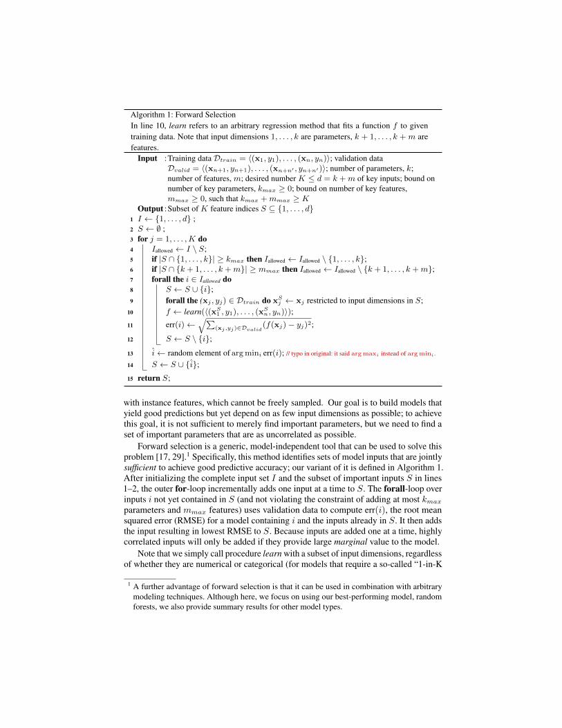
Algorithm 1: Forward SelectionIn line 10, learn refers to an arbitrary regression method that fits a function f to giventraining data. Note that input dimensions 1, . . . , k are parameters, k + 1, . . . , k +m arefeatures.

Input :Training data Dtrain = 〈(x1, y1), . . . , (xn, yn)〉; validation dataDvalid = 〈(xn+1, yn+1), . . . , (xn+n′ , yn+n′)〉; number of parameters, k;number of features, m; desired number K ≤ d = k +m of key inputs; bound onnumber of key parameters, kmax ≥ 0; bound on number of key features,mmax ≥ 0, such that kmax +mmax ≥ K

Output :Subset of K feature indices S ⊆ {1, . . . , d}1 I ← {1, . . . , d} ;2 S ← ∅ ;3 for j = 1, . . . ,K do4 Iallowed ← I \ S;5 if |S ∩ {1, . . . , k}| ≥ kmax then Iallowed ← Iallowed \ {1, . . . , k};6 if |S ∩ {k + 1, . . . , k +m}| ≥ mmax then Iallowed ← Iallowed \ {k + 1, . . . , k +m};7 forall the i ∈ Iallowed do8 S ← S ∪ {i};9 forall the (xj , yj) ∈ Dtrain do xS

j ← xj restricted to input dimensions in S;10 f ← learn(〈(xS

1 , y1), . . . , (xSn, yn)〉);

11 err(i)←√∑

(xj ,yj)∈Dvalid(f(xj)− yj)2;

12 S ← S \ {i};

13 i← random element of argmini err(i); // typo in original: it said argmaxi instead of argmini.

14 S ← S ∪ {i};15 return S;

with instance features, which cannot be freely sampled. Our goal is to build models thatyield good predictions but yet depend on as few input dimensions as possible; to achievethis goal, it is not sufficient to merely find important parameters, but we need to find aset of important parameters that are as uncorrelated as possible.

Forward selection is a generic, model-independent tool that can be used to solve thisproblem [17, 29].1 Specifically, this method identifies sets of model inputs that are jointlysufficient to achieve good predictive accuracy; our variant of it is defined in Algorithm 1.After initializing the complete input set I and the subset of important inputs S in lines1–2, the outer for-loop incrementally adds one input at a time to S. The forall-loop overinputs i not yet contained in S (and not violating the constraint of adding at most kmax

parameters and mmax features) uses validation data to compute err(i), the root meansquared error (RMSE) for a model containing i and the inputs already in S. It then addsthe input resulting in lowest RMSE to S. Because inputs are added one at a time, highlycorrelated inputs will only be added if they provide large marginal value to the model.

Note that we simply call procedure learn with a subset of input dimensions, regardlessof whether they are numerical or categorical (for models that require a so-called “1-in-K

1 A further advantage of forward selection is that it can be used in combination with arbitrarymodeling techniques. Although here, we focus on using our best-performing model, randomforests, we also provide summary results for other model types.

encoding” to handle categorical parameters, this means we introduce/drop all K binarycolumns representing a K-ary categorical input at once). Also note that, while here, weuse prediction RMSE on the validation set to assess the value of adding input i, forwardselection can also be used with any other objective function.2

Having selected a set S of inputs via forward selection, we quantify their relativeimportance following the same process used by Leyton-Brown et al. to determine theimportance of instance features [17], which is originally due to [31]: we simply drop oneinput from S at a time and measure the increase in predictive RMSE. After computingthis increase for each feature, we normalize by dividing by the maximal RMSE increaseand multiplying by 100.

We note that forward selection can be computationally costly due to its need forrepeated model learning: for example, to select 5 out of 200 inputs via forward selectionrequires the construction and validation of 200+199+198+197+196=990 models. In ourexperiments, this process required up to a day of CPU time.

2.3 Selecting Values for Important ParametersGiven a model f that takes k parameters and m instance features as input and predictsa performance value, we identify the best values for the k parameters by optimizingpredictive performance according to the model. Specifically, we predict the performanceof the partial parameter configuration x (instantiating k parameter values) on a probleminstance with m selected instance features z as f([xT, zT]T). Likewise, we predict itsaverage performance across n instances with selected instance features z1, . . . , zn as∑n

j=11n · f([x

T, zTj ]

T).

3 Algorithm Performance DataIn this section, we discuss the algorithm performance data we used in order to evaluate ourapproach. We employ data from three different combinatorial problems: propositionalsatisfiability (SAT), mixed integer programming (MIP), and the traveling salesmanproblem (TSP). All our code and data is available online: instances and their features(and feature computation code & binaries), parameter specification files and wrappersfor the algorithms, as well as the actual runtime data upon which our analysis is based.

3.1 Algorithms and their Configuration SpacesWe employ peformance data from three algorithms: CPLEX for MIP, SPEAR for SAT, andLK-H for TSP. The parameter configuration spaces of these algorithms are summarizedin Table 1.

IBM ILOG CPLEX [32] is the most-widely used commercial optimization tool forsolving MIPs; it is used by over 1 300 corporations (including a third of the Global 500)and researchers at more than 1 000 universities. We used the same configuration spacewith 76 parameters as in previous work [1], excluding all CPLEX settings that changethe problem formulation (e.g., the optimality gap below which a solution is consideredoptimal). Overall, we consider 12 preprocessing parameters (mostly categorical); 17MIP strategy parameters (mostly categorical); 11 categorical parameters deciding howaggressively to use which types of cuts; 9 real-valued MIP “limit” parameters; 10

2 In fact, it also applies to classification algorithms and has, e.g., been used to derive classifiersfor predicting the solubility of SAT instances based on 1–2 features [30].

Algorithm Parameter type # parameters of this type # values considered Total # configurations

Boolean 6 2CPLEX Categorical 45 3–7 1.90 × 1047

Integer 18 5–7Continuous 7 5–8

Categorical 10 2–20SPEAR Integer 4 5–8 8.34 × 1017

Continuous 12 3–6

Boolean 5 2LK-H Categorical 8 3–10 6.91 × 1014

Integer 10 3–9

Table 1. Algorithms and their parameter configuration spaces studied in our experiments.

simplex parameters (half of them categorical); 6 barrier optimization parameters (mostlycategorical); and 11 further parameters. In total, and based on our discretization ofcontinuous parameters, these parameters gave rise to 1.90× 1047 unique configurations.

SPEAR [33] is a state-of-the-art SAT solver for industrial instances. With appropriateparameter settings, it was shown to be the best available solver for certain types ofSAT-encoded hardware and software verification instances [8] (the same IBM and SWV

instances we use here). It also won the quantifier-free bit-vector arithmetic category ofthe 2007 Satisfiability Modulo Theories Competition. We used exactly the same 26-dimensional parameter configuration space as in previous work [8]. SPEAR’s categoricalparameters mainly control heuristics for variable and value selection, clause sorting,resolution ordering, and also enable or disable optimizations, such as the pure literal rule.Its numerical parameters mainly deal with activity, decay, and elimination of variablesand clauses, as well as with the randomized restart interval and percentage of randomchoices. In total, and based on our discretization of continuous parameters, SPEAR has8.34× 1017 different configurations.

LK-H [34] is a state-of-the-art local search solver for TSP based on an efficientimplementation of the Lin-Kernighan heuristic. We used the LK-H code from Styleset al. [35], who first reported algorithm configuration experiments with LK-H; in theirwork, they extended the official LK-H version 2.02 to allow several parameters to scalewith instance size and to make use of a simple dynamic restart mechanism to preventstagnation. The modified version has a total of 23 parameters governing all aspects of thesearch process, with an emphasis on parameterizing moves. In total, and based on ourdiscretization of continuous parameters, LK-H has 6.91× 1014 different configurations.

3.2 Benchmark Instances and their Features

We used the same benchmark distributions and features as in previous work [23] andonly describe them on a high level here. For MIP, we used two instance distributionsfrom computational sustainability (RCW and CORLAT), one from winner determinationin combinatorial auctions (REG), two unions of these (CR := CORLAT ∪ RCW and CRR :=CORLAT ∪ REG ∪ RCW), and a large and diverse set of publicly available MIP instances(BIGMIX). We used 121 features to characterize MIP instances, including features de-scribing problem size, the variable-constraint graph, the constraint matrix, the objectivefunction values, an LP programming relaxation, various probing features extracted fromshort CPLEX runs and timing features measuring the computational expense required forvarious groups of features.

For SAT, we used three sets of SAT-encoded formal verification benchmarks: SWVand IBM are sets of software and hardware verification instances, and SWV-IBM is theirunion. We used 138 features to characterize SAT instances, including features describingproblem size, three graph representations, syntactic features, probing features based onsystematic solvers (capturing unit propagation and clause learning) and local searchsolvers, an LP relaxation, survey propagation, and timing features.

For TSP, we used TSPLIB, a diverse set of prominent TSP instances, and computed64 features, including features based on problem size, cost matrix, minimum spanningtrees, branch & cut probing, local search probing, ruggedness, and node distribution, aswell as timing features.

3.3 Data AcquisitionWe gathered a large amount of runtime data for these solvers by executing them withvarious configurations and instances. Specifically, for each combination of solver andinstance distribution (CPLEX run on MIP, SPEAR on SAT, and LK-H on TSP instances), wemeasured the runtime of each ofM = 1000 randomly-sampled parameter configurationson each of the P problem instances available for the distribution, with P ranging from63 to 2 000. The resulting runtime observations can be thought of as a M × P matrix.Since gathering this runtime matrix meant performing M · P (i.e., between 63 000 and2 000 000) runs per dataset, we limited each single algorithm run to a cutoff time of300 CPU seconds on one node of the Westgrid cluster Glacier (each of whose nodes isequipped with two 3.06 GHz Intel Xeon 32-bit processors and 2–4GB RAM). Whilecollecting this data required substantial computational resources (between 1.3 CPUyears and 18 CPU years per dataset), we note that this much data was only requiredfor the thorough empirical analysis of our methods; in practice, our methods are oftensurprisingly accurate based on small amounts of training data. For all our experiments,we partitioned both instances and parameter configurations into training, validation, andtest sets; the training sets (and likewise, the validation and test sets) were formed assubsamples of training instances and parameter configurations. We used 10 000 trainingsubsamples throughout our experiments but demonstrate in Section 4.3 that qualitativelysimilar results can also be achieved based on subsamples of 1 000 data points.

We note that sampling parameter configurations uniformly at random is not theonly possible way of collecting training data. Uniform sampling has the advantage ofproducing unbiased training data, which in turn gives rise to models that can be expectedto perform well on average across the entire configuration space. However, becausealgorithm designers typically care more about regions of the configuration space thatyield good performance, in future work, we also aim to study models based on datagenerated through a biased sequential sampling approach (as is implemented, e.g., inmodel-based algorithm configuration methods, such as SMAC [6]).

4 Experiments

We carried out various computational experiments to identify the quality of modelsbased on small subsets of features and parameters identified using forward selection,to quantify which inputs are most important, and to determine good values for theselected parameters. All our experiments made use of the algorithm performance datadescribed in Section 3, and consequently, our claims hold on average across the entire

CPLEX-BIGMIX SPEAR-SWV LK-H-TSPLIB

Con

figur

atio

nsp

ace

0 2 4 6 8 10

0

0.01

0.02

0.03

0.04

0.05

Parameter subset size

RM

SE

0 2 4 6 8 10

0

0.05

0.1

0.15

0.2

Parameter subset size

RM

SE

0 2 4 6 8 10

0

0.05

0.1

0.15

0.2

Parameter subset size

RM

SE

Feat

ure

spac

e

0 2 4 6 8 10

0

0.1

0.2

0.3

0.4

0.5

0.6

Feature subset size

RM

SE

0 2 4 6 8 10

0

0.2

0.4

0.6

0.8

1

1.2

1.4

1.6

Feature subset size

RM

SE

0 2 4 6 8 10

0

0.05

0.1

0.15

0.2

0.25

0.3

Feature subset size

RM

SE

Com

bine

dsp

ace

0 2 4 6 8 100

0.2

0.4

0.6

0.8

1

Feature/parameter subset size

RM

SE

0 2 4 6 8 100

0.2

0.4

0.6

0.8

1

1.2

1.4

1.6

Feature/parameter subset size

RM

SE

0 2 4 6 8 100

0.2

0.4

0.6

0.8

1

1.2

1.4

1.6

1.8

Feature/parameter subset sizeR

MS

E

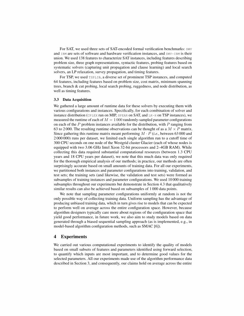
Fig. 1. Predictive quality of random forest models as a function of the number of allowed parame-ters/features selected by forward selection for 3 example datasets. The inputless prediction (subsetsize zero) is the mean of all data points. The dashed horizontal line in each plot indicates the finalperformance of the model using the full set of parameters/features.

configuration space. Whether they also apply to biased samples from the configurationspace (in particular, regions of very strong algorithm performance) is a question forfuture work.

4.1 Predictive Performance for Small Subsets of Inputs

First, we demonstrate that forward selection identifies sets of inputs yielding low predic-tive root mean squared error (RMSE), for predictions in the feature space, the parameterspace, and their joint space. Figure 1 shows the root mean squared error of models fitwith parameter/feature subsets of increasing size. Note in particular the horizontal line,giving the RMSE of a model based on all inputs, and that the RMSE of subset modelsalready converges to this performance with few inputs. In the feature space, this has beenobserved before [17, 29] and is intuitive, since the features are typically very correlated,allowing a subset of them to represent the rest. However, the same cannot be said forthe parameter space: in our experimental design, parameter values have been sampleduniformly at random and are thus independent (i.e., uncorrelated) by design. Thus, thisfinding indicates that some parameters influence performance much more than others, tothe point where knowledge of a few parameter values suffices to predict performancejust as well as knowledge of all parameters.

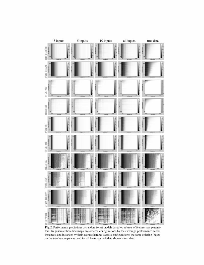
Figure 2 focuses on what we consider to be the most interesting case, namely perfor-mance prediction in the joint space of instance features and parameter configurations.

3 inputs 5 inputs 10 inputs all inputs true dataCPLEX

-BIGMIX

configura

tions

instances

easy hard

good

bad−2

−1.5

−1

−0.5

0

0.5

1

1.5

2

configura

tions

instances

easy hard

good

bad−2

−1.5

−1

−0.5

0

0.5

1

1.5

2

configura

tions

instances

easy hard

good

bad−2

−1.5

−1

−0.5

0

0.5

1

1.5

2

configura

tions

instances

easy hard

good

bad−2

−1.5

−1

−0.5

0

0.5

1

1.5

2

configura

tions

instances

easy hard

good

bad−2

−1.5

−1

−0.5

0

0.5

1

1.5

2

CPLEX

-CORLAT

configura

tions

instances

easy hard

good

bad−2

−1.5

−1

−0.5

0

0.5

1

1.5

2

configura

tions

instances

easy hard

good

bad−2

−1.5

−1

−0.5

0

0.5

1

1.5

2

configura

tions

instances

easy hard

good

bad−2

−1.5

−1

−0.5

0

0.5

1

1.5

2

configura

tions

instances

easy hard

good

bad−2

−1.5

−1

−0.5

0

0.5

1

1.5

2

configura

tions

instances

easy hard

good

bad−2

−1.5

−1

−0.5

0

0.5

1

1.5

2

CPLEX

-RCW

configura

tions

instances

easy hard

good

bad0.5

1

1.5

2

configura

tions

instances

easy hard

good

bad0.5

1

1.5

2

configura

tions

instances

easy hard

good

bad0.5

1

1.5

2

configura

tions

instances

easy hard

good

bad0.5

1

1.5

2

configura

tions

instances

easy hard

good

bad0.5

1

1.5

2

CPLEX

-REG

configura

tions

instances

easy hard

good

bad0.5

1

1.5

2

configura

tions

instances

easy hard

good

bad0.5

1

1.5

2

configura

tions

instances

easy hard

good

bad0.5

1

1.5

2

configura

tions

instances

easy hard

good

bad0.5

1

1.5

2

configura

tions

instances

easy hard

good

bad0.5

1

1.5

2

CPLEX

-CR

configura

tions

instances

easy hard

good

bad−2

−1.5

−1

−0.5

0

0.5

1

1.5

2

configura

tions

instances

easy hard

good

bad−2

−1.5

−1

−0.5

0

0.5

1

1.5

2

configura

tions

instances

easy hard

good

bad−2

−1.5

−1

−0.5

0

0.5

1

1.5

2configura

tions

instances

easy hard

good

bad−2

−1.5

−1

−0.5

0

0.5

1

1.5

2

configura

tions

instances

easy hard

good

bad−2

−1.5

−1

−0.5

0

0.5

1

1.5

2

CPLEX

-CRR

configura

tions

instances

easy hard

good

bad−2

−1.5

−1

−0.5

0

0.5

1

1.5

2

configura

tions

instances

easy hard

good

bad−2

−1.5

−1

−0.5

0

0.5

1

1.5

2

configura

tions

instances

easy hard

good

bad−2

−1.5

−1

−0.5

0

0.5

1

1.5

2

configura

tions

instances

easy hard

good

bad−2

−1.5

−1

−0.5

0

0.5

1

1.5

2

configura

tions

instances

easy hard

good

bad−2

−1.5

−1

−0.5

0

0.5

1

1.5

2

SPEAR

-SWV

configura

tions

instances

easy hard

good

bad−2

−1.5

−1

−0.5

0

0.5

1

1.5

2

configura

tions

instances

easy hard

good

bad−2

−1.5

−1

−0.5

0

0.5

1

1.5

2

configura

tions

instances

easy hard

good

bad−2

−1.5

−1

−0.5

0

0.5

1

1.5

2

configura

tions

instances

easy hard

good

bad−2

−1.5

−1

−0.5

0

0.5

1

1.5

2

configura

tions

instances

easy hard

good

bad−2

−1.5

−1

−0.5

0

0.5

1

1.5

2

SPEAR

-IBM

configura

tions

instances

easy hard

good

bad−2

−1.5

−1

−0.5

0

0.5

1

1.5

2

configura

tions

instances

easy hard

good

bad−2

−1.5

−1

−0.5

0

0.5

1

1.5

2

configura

tions

instances

easy hard

good

bad−2

−1.5

−1

−0.5

0

0.5

1

1.5

2

configura

tions

instances

easy hard

good

bad−2

−1.5

−1

−0.5

0

0.5

1

1.5

2

configura

tions

instances

easy hard

good

bad−2

−1.5

−1

−0.5

0

0.5

1

1.5

2

SPEAR

-IBM

-SWV

configura

tions

instances

easy hard

good

bad−2

−1.5

−1

−0.5

0

0.5

1

1.5

2

configura

tions

instances

easy hard

good

bad−2

−1.5

−1

−0.5

0

0.5

1

1.5

2

configura

tions

instances

easy hard

good

bad−2

−1.5

−1

−0.5

0

0.5

1

1.5

2

configura

tions

instances

easy hard

good

bad−2

−1.5

−1

−0.5

0

0.5

1

1.5

2

configura

tions

instances

easy hard

good

bad−2

−1.5

−1

−0.5

0

0.5

1

1.5

2

LK-H

-TSPLIB

configura

tions

instances

easy hard

good

bad−2

−1.5

−1

−0.5

0

0.5

1

1.5

2

configura

tions

instances

easy hard

good

bad−2

−1.5

−1

−0.5

0

0.5

1

1.5

2

configura

tions

instances

easy hard

good

bad−2

−1.5

−1

−0.5

0

0.5

1

1.5

2

configura

tions

instances

easy hard

good

bad−2

−1.5

−1

−0.5

0

0.5

1

1.5

2

configura

tions

instances

easy hard

good

bad−2

−1.5

−1

−0.5

0

0.5

1

1.5

2

Fig. 2. Performance predictions by random forest models based on subsets of features and parame-ters. To generate these heatmaps, we ordered configurations by their average performance acrossinstances, and instances by their average hardness across configurations; the same ordering (basedon the true heatmap) was used for all heatmaps. All data shown is test data.

The figure qualitatively indicates the performance that can be achieved based on subsetsof inputs of various sizes. We note that in some cases, in particular in the SPEAR scenarios,predictions of models using all inputs closely resemble the true performance, and that thepredictions of models based on a few inputs tend to capture the salient characteristics ofthe full models. Since the instances we study vary widely in hardness, instance featurestend to be more predictive than algorithm parameters, and are thus favoured by forwardselection. This sometimes leads to models that only rely on instance features, yieldingpredictions that are constant across parameter configurations; for example, see the pre-dictions with up to 10 inputs for dataset CPLEX-CORLAT (the second row in Figure 2).While these models yield low RMSE, they are uninformative about parameter settings;this observation caused us to modify forward selection as discussed in Section 2.2 tolimit the number of features/parameters selected.

4.2 Relative Importance of Parameters and FeaturesAs already apparent from Figure 1, knowing the values of a few parameters is sufficientto predict marginal performance across instances similarly well as when knowing allparameter values. Figure 3 shows which parameters were found to be important in differ-ent runs of our procedure. Note that the set of selected key parameters was remarkablyrobust across runs.

The most extreme case is SPEAR-SWV, for which SPEAR’s variable selection heuristic(sp-var-dec-heur) was found to be the most important parameter every single timeby a wide margin, followed by its phase selection heuristic (sp-phase-dec-heur). Theimportance of the variable selection heuristic for SAT solvers is well known, but it issurprising that the importance of this choice dominates so clearly. Phase selection isalso widely known to be important for the performance of modern CDCL SAT solverslike SPEAR. As can be seen from Figure 1 (top middle), predictive models for SPEAR-SWVbased on 2 parameters essentially performed as well as those based on all parameters, asis also reflected in the very low importance ratings for all but these two parameters.

In the case of both CPLEX-BIGMIX and LK-H-TSPLIB, up to 5 parameters show up asimportant, which is not surprising, considering that predictive performance of subsetmodels with 5 inputs converged to that of models with all inputs (see Figure 1, top leftand right). In the case of CPLEX, the key parameters included two controlling CPLEX’scutting strategy (mip limits cutsfactor and mip limits cutpasses, limiting the numberof cuts to add, and the number of cutting plane passes, respectively), two MIP strategyparameters (mip strategy subalgorithm and mip strategy variableselect, determiningthe continuous optimizer used to solve subproblems in a MIP, and variable selection,respectively), and one parameter determining which kind of reductions to perform duringpreprocessing (preprocessing reduce). In the case of LK-H, all top five parameters arerelated to moves, parameterizing candidate edges (EXCESS and MAX CANDIDATES,limiting the maximum alpha-value allowed for any candidate edge, and the maximumnumber of candidate edges, respectively), and move types (MOVE TYPE, BACK-TRACKING, SUBSEQUENT MOVE TYPE, specifying whether to use sequentialk-opt moves, whether to use backtracking moves, and which type to use for movesfollowing the first one in a sequence of moves).

To demonstrate the model independence of our approach, we repeated the sameanalysis based on other empirical performance models (linear regression, neural net-works, Gaussian processes, and regression trees). Although overall, these models yielded

0 20 40 60 80 100

preprocessing_dual

simplex_crash

sifting_algorithm

mip_strategy_backtrack

simplex_refactor

mip_limits_cutpasses

preprocessing_reduce

mip_strategy_variableselect

mip_strategy_subalgorithm

mip_limits_cutsfactor

Importance

(a) CPLEX-BIGMIX

0 20 40 60 80 100

sp−restart−inc

sp−rand−phase−dec−freq

sp−update−dec−queue

sp−rand−var−dec−scaling

sp−resolution

sp−var−activity−inc

sp−rand−var−dec−freq

sp−variable−decay

sp−phase−dec−heur

sp−var−dec−heur

Importance

(b) SPEAR-SWV

0 50 100

RUNS

MAX_BREADTH

PATCHING_C_OPTIONS

STABLE_RUNS

MAX_CANDIDATES_SYMMETRIC

MOVE_TYPE

BACKTRACKING

SUBSEQUENT_MOVE_TYPE

MAX_CANDIDATES

EXCESS

Importance

(c) LK-H-TSPLIBFig. 3. Parameter importance for 3 example datasets. We show boxplots over 10 repeated runswith different random training/validation/test splits.

Dataset CPLEX-BIGMIX SPEAR-SWV LK-H-TSPLIB

1st selected cplex prob time (10.1) Pre featuretime (35.9) tour const heu avg (0.0)2nd selected obj coef per constr2 std (7.7) nclausesOrig (100.0) cluster distance std (0.8)3rd selected vcg constr weight0 avg (30.2) sp-var-dec-heur (32.6) EXCESS (10.0)4th selected mip limits cutsfactor (8.3) VCG CLAUSE entropy (34.5) bc no1s q25 (100.0)5th selected mip strategy subalgorithm (100.0) sp-phase-dec-heur (27.6) BACKTRACKING (0.0)

Table 2. Key inputs, in the order in which they were selected, along with their omission cost fromthis set.

weaker predictions, the results were qualitatively similar: for SPEAR, all models reliablyidentified the same two parameters as most important, and for the other datasets, therewas an overlap of at least three of the top five ranked parameters. Since random forestsyielded the best predictive performance, we focus on them in the remainder of this paper.

As an aside, we note that the fact that a few parameters dominate importance is inline with similar findings in the machine learning literature on the importance of hyper-parameters, which has informed the analysis of a simple hyperparameter optimizationalgorithm [36] and the design of a Bayesian optimization variant for optimizing functionswith high extrinsic but low intrinsic dimensionality [37]. In future work, we plan toexploit this insight to design better automated algorithm configuration procedures.

Next, we demonstrate how we can study the joint importance of instance features andalgorithm parameters. Since foward selection by itself chose mostly instance features,for this analysis we constrained it to select 3 features and 2 parameters. Table 2 liststhe features and parameters identified for our 3 example datasets, in the order forwardselection picked them. Since most instance features are strongly correlated with eachother, it is important to measure and understand our importance metric in the context ofthe specific subset of inputs it is computed for. For example, consider the set of importantfeatures for dataset CPLEX-BIGMIX (Table 2, left). While the single most important featurein this case was cplex prob time (a timing feature measuring how long CPLEX probingtakes), in the context of the other four features, its importance was relatively small; onthe other hand, the input selected 5th, mip strategy subalgorithm (CPLEX’s MIP strategyparameter from above) was the most important input in the context of the other 4. Wealso note that all algorithm parameters that were selected as important in this contextof instance features (mip limits cutsfactor and mip strategy subalgorithm for CPLEX;sp-var-dec-heur and sp-phase-dec-heur for SPEAR; and EXCESS and BACKTRACKINGfor LK-H) were already selected and labeled important when considering only parameters.This finding increases our confidence in the robustness of this analysis.

Dataset 1st selected param 2nd selected param

CPLEX-BIGMIX mip limits cutsfactor = 8 mip strategy subalgorithm = 2CPLEX-CORLAT mip strategy subalgorithm = 2 preprocessing reduce = 3CPLEX-REG mip strategy subalgorithm = 2 mip strategy variableselect = 4CPLEX-RCW preprocessing reduce = 3 mip strategy lbheur = noCPLEX-CR mip strategy subalgorithm = 0 preprocessing reduce = 1CPLEX-CRR preprocessing coeffreduce = 2 mip strategy subalgorithm = 2

SPEAR-IBM sp-var-dec-heur = 2 sp-resolution = 0SPEAR-SWV sp-var-dec-heur = 2 sp-phase-dec-heur = 0SPEAR-SWV-IBM sp-var-dec-heur = 2 sp-use-pure-literal-rule = 0

LK-H-TSPLIB EXCESS = -1 BACKTRACKING = NO

Table 3. Key parameters and their best fixed values as judged by an empirical performance modelbased on 3 features and 2 parameters.

4.3 Selecting Values for Key Parameters

Next, we used our subset models to identify which values the key parameters identifiedby forward selection should be set to. For each dataset, we used the same subset modelsof 3 features and 2 parameters as above; Table 3 lists the best predicted values for these2 parameters. The main purpose of this experiment was to demonstrate that this analysiscan be done automatically, and we thus only summarize the results at a high level; wesee them as a starting point that can inform domain experts about empirical properties oftheir algorithm in a particular application context and trigger further in-depth studies. Ata high level, we note that CPLEX’s parameter mip strategy subalgorithm (determiningthe continuous optimizer used to solve subproblems in a MIP) was important for mostinstance sets, the most prominent values being 2 (use CPLEX’s dual simplex optimizer)and 0 (use CPLEX’s auto-choice, which also defaults to the dual simplex optimizer).Another important choice was to set preprocessing reduce to 3 (use both primal and dualreductions) or 1 (use only primal reductions), depending on the instance set. For SPEAR,the parameter determining the variable selection heuristic (sp-var-dec-heur) was the mostimportant one in all 3 cases, with an optimal value of 2 (select variables based on theiractivity level, breaking ties by selecting the more frequent variable). For good averageperformance of LK-H on TSPLIB, the most important choices were to set EXCESS to -1(use an instance-dependent setting of the reciprocal problem dimension), and to not usebacktracking moves.

We also measured the performance of parameter configurations that actually setthese parameters to the values predicted to be best by the model, both on average acrossinstances and in an instance-specific way. This serves as a further way of evaluating modelquality and also facilitates deeper understanding of the parameter space. Specifically, weconsider parameter configurations that instantiate the selected parameters according tothe model and assign all other parameter to randomly sampled values; we compare theperformance of these configurations to that of configurations that instantiate all valuesat random. Figure 4 visualizes the result of this comparison for two datasets, showingthat the model indeed selected values that lead to high performance: by just controllingtwo parameters, improvements of orders of magnitude could be achieved for someinstances. Of course, this only compares to random configurations; in contrast to ourwork on algorithm configuration, here, our goal was to gain a better understanding of analgorithms’ parameter space rather than to improve over its manually engineered default

102.3

102.4

102.5

102.3

102.4

102.5

Avg. perf. [CPU s]

Pe

rf.

of

be

st

an

d b

est

pe

r in

sta

nce

[C

PU

s]

Single best

Per−instance

(a) CPLEX-RCW

10−2

10−1

100

101

102

10−2

10−1

100

101

102

Avg. perf. [CPU s]

Pe

rf.

of

be

st

an

d b

est

pe

r in

sta

nce

[C

PU

s]

Single best

Per−instance

(b) SPEAR-SWVFig. 4. Performance of random configurations vs configurations setting almost all parameters atrandom, but setting 2 key parameters based on an empirical performance model with 3 featuresand 2 parameters.

CPLEX-BIGMIX CPLEX-CORLAT CPLEX-RCW CPLEX-REG SPEAR-IBM SPEAR-SWV LK-H-TSPLIB

1000

0da

tapo

ints

−2

−1

0

1

2

3

4

best p.i.−2

−1

0

1

2

3

4

best p.i.−2

−1

0

1

2

3

4

best p.i.−2

−1

0

1

2

3

4

best p.i.−2

−1

0

1

2

3

4

best p.i.−2

−1

0

1

2

3

4

best p.i.−2

−1

0

1

2

3

4

best p.i.

100

0da

tapo

ints

−2

−1

0

1

2

3

4

best p.i.−2

−1

0

1

2

3

4

best p.i.−2

−1

0

1

2

3

4

best p.i.−2

−1

0

1

2

3

4

best p.i.−2

−1

0

1

2

3

4

best p.i.−2

−1

0

1

2

3

4

best p.i.−2

−1

0

1

2

3

4

best p.i.

Fig. 5. Log10 speedups over random configurations by setting almost all parameters at random,except 2 key parameters, values for which (fixed best, and best per instance) are selected by anempirical performance model with 3 features and 2 parameters. The boxplots show the distributionof log10 speedups across all problem instances; note that, e.g., a log10 speedup of 0, -1, and 1mean identical performance, a 10-fold slowdown, and a 10-fold speedup, respectively. The dashedgreen lines indicate where two configurations performed the same, points above the line indicatespeedups. Top: based on models trained on 10 000 data points; bottom: based on models trainedon 1 000 data points.

parameter settings.3 However, we nevertheless believe that the speedups achieved bysetting only the identified parameters to good values demonstrate the importance of theseparameters. While Figure 4 only covers 2 datasets, Figure 5 (top) summarizes results fora wide range of datasets. Figure 5 (bottom) demonstrates that predictive performancedoes not degrade much when using sparser training data (here: 1 000 instead of 10 000training data points); this is important for facilitating the use of our approach in practice.

3 In fact, in many cases, the best setting of the key parameters were their default values.

5 Conclusions

In this work, we have demonstrated how forward selection can be used to analyzealgorithm performance data gathered using randomly sampled parameter configurationson a large set of problem instances. This analysis identified small sets of key algorithmparameters and instance features, based on which the performance of these algorithmscould be predicted with surprisingly high accuracy. Using this fully automated analysistechnique, we found that for high-performance solvers for some of the most widelystudied NP-hard combinatorial problems, namely SAT, MIP and TSP, only very fewkey parameters (often just two of dozens) largely determine algorithm performance.Automatically constructed performance models, in our case based on random forests,were of sufficient quality to reliably identify good values for these key parameters,both on average across instances and dependent on key instance features. We believethat our rather simple importance analysis approach can be of great value to algorithmdesigners seeking to identify key algorithm parameters, instance features, and theirinteraction. We also note that the finding that the performance of these highly parametricalgorithms mostly depends on a few key parameters has broad implications on the designof algorithms for NP-hard problems, such as the ones considered here, and of futurealgorithm configuration procedures.

In future work, we aim to reduce the computational cost of identifying key param-eters; to automatically identify the relative performance obtained with their possiblevalues; and to study which parameters are important in high-performing regions of analgorithm’s configuration space.

References

[1] F. Hutter, H. H. Hoos, and K. Leyton-Brown. Automated configuration of mixed integerprogramming solvers. In Proc. of CPAIOR-10, pages 186–202, 2010.

[2] V. Nannen and A. E. Eiben. Relevance estimation and value calibration of evolutionaryalgorithm parameters. In Proc. of IJCAI-07, pages 975–980, 2007.

[3] C. Ansotegui, M. Sellmann, and K. Tierney. A gender-based genetic algorithm for theautomatic configuration of solvers. In Proc. of CP-09, pages 142–157, 2009.

[4] M. Birattari, Z. Yuan, P. Balaprakash, and T. Stutzle. In T. Bartz-Beielstein, M. Chiarandini,L. Paquete, and M. Preuss, editors, Empirical Methods for the Analysis of OptimizationAlgorithms, chapter F-race and iterated F-race: An overview. Springer, 2010.

[5] F. Hutter, H. H. Hoos, K. Leyton-Brown, and T. Stutzle. ParamILS: an automatic algorithmconfiguration framework. JAIR, 36:267–306, October 2009.

[6] F. Hutter, H. H. Hoos, and K. Leyton-Brown. Sequential model-based optimization forgeneral algorithm configuration. In Proc. of LION-5, pages 507–523, 2011.

[7] F. Hutter, H. H. Hoos, and K.Leyton-Brown. Parallel algorithm configuration. In Proc. ofLION-6, pages 55–70, 2012.

[8] F. Hutter, D. Babic, H. H. Hoos, and A. J. Hu. Boosting verification by automatic tuning ofdecision procedures. In Proc. of FMCAD-07, pages 27–34, 2007.

[9] M. Chiarandini, C. Fawcett, and H. Hoos. A modular multiphase heuristic solver for postenrolment course timetabling. In Proc. of PATAT-08. 2008.

[10] M. Vallati, C. Fawcett, A. E. Gerevini, H. H. Hoos, and Alessandro Saetti. Generating fastdomain-optimized planners by automatically configuring a generic parameterised planner.In Proc. of ICAPS-PAL11, 2011.

[11] E. Ridge and D. Kudenko. Sequential experiment designs for screening and tuning parametersof stochastic heuristics. In Proc. of PPSN-06, pages 27–34, 2006.

[12] M. Chiarandini and Y. Goegebeur. Mixed models for the analysis of optimization algorithms.In T. Bartz-Beielstein, M. Chiarandini, L. Paquete, and M. Preuss, editors, ExperimentalMethods for the Analysis of Optimization Algorithms, pages 225–264. Springer Verlag, 2010.

[13] T. Bartz-Beielstein. Experimental research in evolutionary computation: the new experimen-talism. Natural Computing Series. Springer Verlag, 2006.

[14] U. Finkler and K. Mehlhorn. Runtime prediction of real programs on real machines. InProc. of SODA-97, pages 380–389, 1997.

[15] E. Fink. How to solve it automatically: Selection among problem-solving methods. InProc. of AIPS-98, pages 128–136. AAAI Press, 1998.

[16] A. E. Howe, E. Dahlman, C. Hansen, M. Scheetz, and A. Mayrhauser. Exploiting competitiveplanner performance. In Proc. of ECP-99, pages 62–72. 2000.

[17] K. Leyton-Brown, E. Nudelman, and Y. Shoham. Learning the empirical hardness ofoptimization problems: the case of combinatorial auctions. In Proc. of CP-02, pages 556–572, 2002.

[18] J. R. Rice. The algorithm selection problem. Advances in Computers, 15:65–118, 1976.[19] K. Smith-Miles. Cross-disciplinary perspectives on meta-learning for algorithm selection.

ACM Computing Surveys, 41(1):6:1–6:25, 2009.[20] K. Smith-Miles and L. Lopes. Measuring instance difficulty for combinatorial optimization

problems. Computers and Operations Research, 39(5):875–889, 2012.[21] L. Xu, F. Hutter, H. H. Hoos, and K. Leyton-Brown. SATzilla: portfolio-based algorithm

selection for SAT. JAIR, 32:565–606, June 2008.[22] F. Hutter, Y. Hamadi, H. H. Hoos, and K. Leyton-Brown. Performance prediction and

automated tuning of randomized and parametric algorithms. In Proc. of CP-06, pages213–228, 2006.

[23] F. Hutter, L. Xu, H.H. Hoos, and K. Leyton-Brown. Algorithm runtime prediction: The stateof the art. CoRR, abs/1211.0906, 2012.

[24] K. Smith-Miles and J. van Hemert. Discovering the suitability of optimisation algorithms bylearning from evolved instances. AMAI, 61:87–104, 2011.

[25] T. Bartz-Beielstein and S. Markon. Tuning search algorithms for real-world applications: aregression tree based approach. In Proc. of CEC-04, pages 1111–1118, 2004.

[26] C. M. Bishop. Pattern recognition and machine learning. Springer, 2006.[27] C. E. Rasmussen and C. K. I. Williams. Gaussian processes for machine learning. MIT

Press, 2006.[28] L. Breiman. Random forests. Machine Learning, 45(1):5–32, 2001.[29] K. Leyton-Brown, E. Nudelman, and Y. Shoham. Empirical hardness models: methodology

and a case study on combinatorial auctions. Journal of the ACM, 56(4):1–52, 2009.[30] L. Xu, H. H. Hoos, and K. Leyton-Brown. Predicting satisfiability at the phase transition. In

Proc. of AAAI-12, 2012.[31] J. Friedman. Multivariate adaptive regression splines. Annals of Statistics, 19(1):1–141,

1991.[32] IBM Corp. IBM ILOG CPLEX Optimizer. http://www-01.ibm.com/software/integration/

optimization/cplex-optimizer/, 2012. Last accessed on October 27, 2012.[33] D. Babic and F. Hutter. Spear theorem prover. Solver description, SAT competition, 2007.[34] K. Helsgaun. General k-opt submoves for the Lin-Kernighan TSP heuristic. Mathematical

Programming Computation, 1(2-3):119–163, 2009.[35] J. Styles, H. H. Hoos, and M. Muller. Automatically configuring algorithms for scaling

performance. In Proc. of LION-6, pages 205–219, 2012.[36] J. Bergstra and Y. Bengio. Random search for hyper-parameter optimization. JMLR, 13:281–

305, 2012.[37] Z. Wang, M. Zoghi, F. Hutter, D. Matheson, and N. de Freitas. Bayesian Optimization in a Bil-

lion Dimensions via Random Embeddings. ArXiv e-prints, January 2013. arXiv:1301.1942.