Identifying Agglomeration Spillovers: Evidence from ...webfac/dromer/e291_f07/Moretti.pdf ·...
52
Identifying Agglomeration Spillovers: Evidence from Million Dollar Plants* Michael Greenstone Richard Hornbeck Enrico Moretti August 2007 *We thank Chad Syverson and seminar participants at the NBER Summer Institute and Stanford for useful comments. The research in this paper was conducted while one of the authors was a Census Bureau research associate at the Boston Census Research Data Center. Research results and conclusions expressed are those of the authors and do not necessarily indicate concurrence by the Bureau of Census. All the tables and figures in this paper have been screened by the Census to insure that no confidential data is revealed.
Transcript of Identifying Agglomeration Spillovers: Evidence from ...webfac/dromer/e291_f07/Moretti.pdf ·...

Identifying Agglomeration Spillovers:
Evidence from Million Dollar Plants*
Michael Greenstone
Richard Hornbeck
Enrico Moretti
August 2007
*We thank Chad Syverson and seminar participants at the NBER Summer Institute and Stanford for useful comments. The research in this paper was conducted while one of the authors was a Census Bureau research associate at the Boston Census Research Data Center. Research results and conclusions expressed are those of the authors and do not necessarily indicate concurrence by the Bureau of Census. All the tables and figures in this paper have been screened by the Census to insure that no confidential data is revealed.

Identifying Agglomeration Spillovers: Evidence from Million Dollar Plants
We quantify agglomeration spillovers by estimating how the productivity of incumbent manufacturing plants in a county varies when a new plant opens in that county. To do so we augment standard Cobb-Douglas production functions for incumbent establishments by allowing total factor productivity to depend on the presence of the new plant. We rely on the revealed rankings of profit-maximizing firms to identify a valid counterfactual for what would have happened in the absence of the plant opening. These rankings reveal the county where the new firm ultimately chose to locate (i.e., the 'winner'), as well as the one or two runner-up counties (i.e., the 'losers'). We find that in the 7 years before the new plant opening, trends in total factor productivity of incumbent plants in winning and losing counties are remarkably similar. But after the opening of the new plant, incumbent plants in winning counties experience a sharp increase in total factor productivity. The plant opening is associated with a 13% increase in incumbent plants TFP five years later. This effect is even larger for incumbent plants that are in the same 2-digit industry of the new plant. We also find that spillovers are larger for pair of industries that are linked by intense flows of workers mobility and pair of industries that employ similar technologies. Michael Greenstone MIT Department of Economics 50 Memorial Drive, E52-359 Cambridge, MA 02142-1347 and NBER [email protected] Richard Hornbeck MIT Department of Economics E52-391 77 Massachusetts Avenue Cambridge MA 02142-1347 [email protected] Enrico Moretti University of California, Berkeley Department of Economics Berkeley, CA 94720-3880 and NBER [email protected]

3
Introduction
Economic activity is spatially concentrated. Economists have speculated for at least a century that
the spatial concentration of economic activity may be explained by productivity advantages enjoyed by
firms when they locate near other firms (Marshall, 1920). The mere existence of clusters of economic
activity of the type exemplified by Silicon Valley has long been used to support the notion of such
agglomeration spillovers. Why would firms that produce tradable goods be willing to locate in areas
characterized by high labor and land costs if this type of locations did not provide significant productivity
advantages? Different hypothesis have been advanced to explain geographical concentration of economic
activity:1 better quality of the worker-firm match in thicker labor markets; lower risk of unemployment
for workers and lower risk of unfilled vacancies for firms following idiosyncratic shocks; cheaper and
faster supply of intermediate goods and services; and knowledge spillovers.2
Beside its obvious interest for urban and growth economists, the magnitude of agglomeration
spillovers has tremendous practical relevance. Increasingly, local governments compete by offering
substantial subsidies to industrial plants to locate within their jurisdictions. The main economic rationale
for these incentives rests on whether the attraction of new businesses generates positive agglomeration
externalities. While the attraction of a new business may generate local jobs, in the absence of positive
externalities it difficult to justify the use of taxpayer money for subsidies, at least based on efficiency
grounds.3
How large are productivity spillovers in practice? Despite its enormous theoretical and practical
relevance, the exact magnitude of agglomeration spillovers is still largely an open question. The empirical
challenge in measuring and explaining agglomeration spillovers is that plants choose to locate where their
expected profits are highest, and their profits are a function of their location-specific costs of production.
Local factors that might affect cost of productions include everything from availability of transportation
infrastructure, to labor and environmental regulations, to the availability of workers with particular skills,
to local culture and institutions. Not only are these factors typically difficult to measure, but their relative
importance is likely to vary across firms based on firms� unobserved production functions.
1 See for example Ellison, Glaeser and Kerr (2007), Ottaviano and Thisse (2004), Rosenthal and Stange (2004), Duranton and Puga (2004), Audretsch and Feldman, (1996 and 2004), Davis and Henderson (2004), Henderson and Black (2003), Henderson (2003), Moretti (2004c), Henderson (2001a, 2001b and 2003), Dumais, Ellison and Gleaser (2002), Rosenthal and Stange (2001), Ellison and Gleaser (1997), Glaeser (1999), and Krugman (1991a and 1991b). 2 Of course, natural production advantages of some areas could be in part responsible for agglomeration. But Elllison and Glaeser (1997) show that natural advantages can not account for the total amount of agglomeration observed in the data. 3 See also Card, Hallock and Moretti (2007) and Glaeser, (2001).

4
It is therefore difficult to properly account for all possible factors that determine production costs
and that might be shared by all firms in the same location. As a consequence, it is hard to determine
whether firms cluster in some areas because proximity increases their productivity or because those areas
are simply more attractive than others. For local governments, it is difficult to determine the magnitude of
the optimal incentive package.
In this paper we have two goals. First, we aim to test for and quantify agglomeration spillovers by
estimating how the productivity of incumbent manufacturing plants in a county varies when a new plant
opens in that county. To do so, we estimate production functions using plant-level data from the Annual
Survey of Manufacturers. We augment standard Cobb-Douglas or Translog production functions for
incumbent establishments by allowing total factor productivity to depend on the presence of the new
plant.4 Having found evidence that the opening of a new plant is associated with significant productivity
gains for the incumbent establishment, we then attempt to shed some light on the degree to which the
agglomeration economies are due to alternative channels. To do so, we test whether the spillovers
between two establishments that are in the same county and are economically close are larger than the
spillovers between two establishments that are in the same county but are economically distant. We
perform this test using four alternative definitions of economic proximity in order to identify the
transmission channels of the spillover.
Heterogeneity in the factors that determine variation in costs of production across counties is
likely to bias standard estimators. Valid estimates of the impact of a plant opening require the
identification of a county that is identical to the county where the plant decided to locate. We rely on the
revealed rankings of profit-maximizing firms to identify a valid counterfactual for what would have
happened in the absence of the plant opening. These rankings come from the corporate real estate journal
Site Selection, which includes a regular feature titled the �Million Dollar Plants� that describes how a
large plant decided where to locate. When firms are considering where to open a large plant, they
typically begin by considering dozens of possible locations. They subsequently narrow the list to roughly
10 sites, among which 2 or 3 finalists are selected. The �Million Dollar Plants� articles report the county
that the plant ultimately chose (i.e., the �winner�), as well as the one or two runner-up counties (i.e., the
�losers�). The losers are counties that have survived a long selection process, but narrowly lost the
competition.
Our identifying assumption is that the losers form a valid counterfactual for the winners, after
adjustment for differences in pre-existing trends. Compared to the rest of the country, winning counties
4 The idea of identifying spillovers by estimating plant level production functions is similar to the approach taken by Henderson (2003) and Moretti (2004).

5
have higher rates of growth in income, population and labor force participation. But compared to losing
counties in the years before the opening of the new plant, winning counties have similar trends in most
economic variables. This finding is consistent with our identifying assumption that the losers form a valid
counterfactual for the winners.
We first measure the effect of the new plant on total factor productivity of all existing plants in
the county. We find that in the 7 years before the new plant opening, trends in total factor productivity of
incumbent plants in winning and losing counties are remarkably similar. But after the opening of the new
plant, incumbent plants in winning counties experience a sharp increase in total factor productivity. The
effect is statistically significant and economically substantial. Our models indicate that the plant opening
is associated with a 13% increase in incumbent plants TFP five years later. We interpret this finding as
evidence of existence of significant productivity spillovers generated by increased agglomeration. As one
might expect, this effect is larger for incumbent plants that are in the same 2-digit industry of the new
plant, and smaller for incumbent plants that are in a different 2-digit industry.5
These increases in productivity do not necessarily translate into higher profits. Using a simple
model, we show that incumbent firms in winning counties are expected to face higher prices for land,
non-traded local inputs and, in the case of a not infinitely elastic local labor supply, for labor as well.
Indeed, we find evidence of increases in the quality-adjusted cost of labor following MDP plant openings.
Given that the plants in our sample produce traded goods, it is unlikely that they can raise the price of
their output. Thus, while we can not directly measure it, the increase in profits is likely to be smaller than
the measured gain in TFP. We do find some evidence of positive net entry of manufacturing plants in
winning counties, which is consistent with a positive effect on profits.
Having found evidence in favor of the existence of agglomeration spillovers, in the last part of the
paper we try to shed some light on the possible mechanisms. To do so, we follow Moretti (2004b) and
Ellison, Glaeser and Kerr (2007) and investigate the relationship between economic distance and
spillovers using four direct measures of economic distance. First, we use input-output tables and assume
that the economic distance between two industries is proportional to the value of inputs or outputs that
they exchange. Second, we use an index of technological distance based on the distribution of patents
across technological fields.6 According to this metric, two industries are close if the distribution of patents
across technologies is similar. Third, we use a metric based on linkages revealed by patents citations.7
According to this metric, two industries are close if they often cite the other industry's patents. Finally, we
use a measure of workers mobility across industries that is intended to capture how likely is that a worker
5 Notably, naïve estimates that control for observables but do not use our Million Dollar Plant research design find negative productivity effects. 6 This measure was first proposed by Jaffe (1986). 7 This measure was first proposed by Jaffe and Trajtenberg, 2001.

6
in a given industry moves to another industry. The idea is that we want to see which measures of
economic distance are associated with large spillover effects. For example, finding that the interaction
with the measure of proximity based on workers transitions is large, suggests that spillovers occur
through the flow of workers across firms. On the other hand, finding that the interaction with proximity as
measured by input-output tables is large, suggests that spillovers occur through the exchange of local
goods and services. Of course, these explanations are not mutually exclusive, and it is possible that more
than one is at play.
We find that spillovers are larger for pair of industries between which there is intense flow of
workers. A one standard deviation increase in our measure of workers mobility between incumbent
plants� industry and the new plant industry is associated with a 7.5% increase in the magnitude of the
spillover. Similarly, the measures of technological linkages indicate statistically meaningful increases in
the spillover. Surprisingly, we find little support for the importance of input and output flows in
determining the magnitude of the spillover. Overall, this evidence provides some support for the notion
that spillovers occurs between firms that share workers and use similar technologies. The evidence seems
less consistent with the hypothesis that agglomeration occurs because of geographical proximity to
customers and suppliers.
The rest of the paper is organized as follows. In Section I we present a simple model. In Section
II we discuss our identification strategy. In Section III we present the data sources. In Section IV, we
present the econometric model. In Section V we present our empirical findings. Section VI concludes.
I. A Simple Theoretical Framework
We are interested in identifying how the opening of a new plant in a county affects the
productivity, profits and input use of existing plants in the same county. We begin in this Section by
presenting a simple theoretical framework that might be useful in interpreting the empirical evidence that
we describe in Section V.
A. Model
We begin by considering the case were incumbent firms are homogenous is size and technology.
Later we consider what happens when incumbent firms are heterogeneous. Through the paper we focus
on the case of factor-neutral spillovers.
(a) Homogeneous Incumbents. We assume that all the incumbent firms use a production
technology that depends on labor, capital and land to produce a nationally traded good whose price is
fixed and is normalized to 1. Incumbent firms choose the amount of labor, L, capital, K, and land, T, to
maximize the following expression:

7
Max L,K,T { f[A, L, K, T] � w L � r K � q T }
where w, r and q are input prices and A is a productivity shifter (TFP). Specifically, A includes all factors
that affect the productivity of labor, capital and land equally, such as technology and agglomeration
spillovers, if they exist. In particular, to explicit allow for agglomeration effects, we allow A to depend on
the density of economic activity in an area:
(1) A = A(N)
where N is the number of firms that are active in a county, and all counties have equal size. We define
factor-neutral agglomeration spillovers as the case where A increases in N:
δA /δN >0
If instead (δA /δN) =0, we say that there are no factor neutral agglomeration spillovers.
Let L*(w,r,q) be the optimal level of labor inputs, given the prevailing wage, cost of capital and
cost of industrial land. Similarly, let�s call K*(w,r,q) and T*(w,r,q) the optimal level of capital and land. In
equilibrium, L*, K* and T* are set so that the marginal product of each of the three factors is equal to its
price.
We assume that capital is internationally traded, so that its price does not depend on local demand
or supply conditions. But we allow for the price of labor and land to depend on local economic
conditions. In particular, we allow the supply of labor and land to be less than infinitely elastic at the
county level.
We think of an upward sloping labor supply curve as the result of moving costs. Like in the
standard Roback (1982) model, we assume that workers� indirect utility depends on wages and cost of
housing, and that in equilibrium workers are indifferent across locations. Workers are mobile across
locations, but unlike the standard Roback (1982) model we allow for moving costs. For simplicity, we
ignore labor supply decisions within a given location, and assume that all residents provide a fixed
amount of labor.
Why is labor supply upward sloping? It is because of mobility costs. The number of workers in
county c before the opening of the new plant is m. This number is determined by the distribution of
moving costs of workers in counties other than c. In particular, m is such that, given the distribution of
wages and the housing costs across localities, the marginal worker in a county different from c is
indifferent between moving to county c and staying. When a new plant opens in county c, wages there
start rising, and some workers find it optimal to move to c. The number of workers who move, and
therefore the slope of the labor supply function, depend on the shape of the mobility cost function. Let

8
w(N) be the (inverse of the) reduced form labor supply function, that links the number of firms active in a
county, N, to the local nominal wage level, w.
Similarly, we allow the supply of industrial land to be less than infinitely elastic at the county
level. It is possible that the supply of land is fixed by geographical constraints. Alternatively, it is possible
that it is fixed, at least in the short run, because of land regulations. Alternatively, it may not be
completely fixed, but it is possible that the best industrial land has already been developed, so that the
marginal land is of decreasing quality or more expensive to develop. Irrespective of the reason, we call
q(N) the (inverse of the) reduced form land supply function that links N, to the price of land.
We can therefore write the equilibrium level of profits, Π*, as
Π* = f[ A(N), L*(w(N), r, q(N)), K*(w(N), r, q(N)), T*(w(N), r, q(N)) ] -
- w(N) L*(w(N), r, q(N)) � r K*(w(N), r, q(N)) � q(N) T*(w(N), r, q(N))
where we now make explicit the fact that TFP, wages and land prices depend on the number of firms
active in a county.
We are interested in determining the short run effect of adding an additional firm in county c on
the profits of incumbent firms:
δΠ*/δN = (δf /δA δA/δN) +
(2) +δw/δN { [δL/δw (δf/δL � w) �L] + [δK/δw (δf/δK � r)] + [δT/δw (δf/δT � q)]}+
+ δq/δN { [δL/δq (δf/δL � w)] + [δK/δq (δf/δK � r)] + [δT/δq (δf/δT � q) - T] }
Intuitively, the effect of an increase in N on profits is the sum of two opposite forces. First, if
there are agglomeration spillovers, the productivity of all factors increases. In the equation above, this
effect on TFP is represented by the term (δf /δA δA/δN). This effect is unambiguously positive, because it
allows an incumbent firm to produce more output using the same amount of inputs. Formally, δf /δA >0
by assumption, and δA/δN >0 if there are agglomeration spillovers.
Second, an increase in N affects the price of the factors of production that are not supplied with
infinite elasticity. Intuitively, an increase in N generates an increase in the level of economic activity in
the county, and therefore an increase in the local demand for labor, capital and land. If the supply of labor
and land is not perfectly elastic at the local level, the price of labor and the price of land will increase. Of
course, the increase will depend on the elasticity of supply of labor and land.
Unlike the beneficial effect agglomeration spillovers, the increase in factor prices is bad news for
incumbent firms, because they have now to compete for locally scare resources with the new entrant. The
increase in wages and land prices has two effects on incumbents. First, for a given level of input
utilizations it mechanically raises production costs. Second, it leads the firm to re-optimize and to change
its use of the different production inputs. In particular, given that the price of capital is not affected by an
increase in N, the firm is likely to end up using more capital than before:

9
δK*/δN =>0.
The effect on the use of labor and land is ambiguous. On the one hand the productivity of all
factors increases, but on the other hand the price of labor and land might increase. The net effect depends
on the magnitude of the factor price increases, as well as on the exact shape of the production function
(i.e. technological complementarities between labor, capital and land):
In equilibrium, if all firms are price takers and all factors are paid their marginal product,
equation (2) simplifies considerably and can be re-written as:
(3) δΠ*/δN = (δf /δA δA/δN) - [ δw/δN L + δq/δN T]
Empirically, the short-run effect of the opening of the new plant on incumbent plants can be
either positive or negative, depending on the strength of agglomeration spillovers. Equation (3) makes
clear that the effect of the new plant is the sum of two opposite effects. The first term represents the
positive effect on TFP that stems from agglomeration spillovers. The second term represents the negative
effect that stems from increases in the cost of labor and land. All the other terms in equation (2) drop
because in equilibrium the firm is choosing its input level optimally, irrespective of the price of inputs. Of
course, if the supply of labor is infinitely elastic at the local level, and if the supply of land is also very
elastic, the effect of a plant opening on incumbent can only be positive.
In the long run, if the net effect on profits is positive, one may expect entry of new firms in the
area. These new firms are willing to pay higher wages and higher land prices to enjoy the benefits of
increased agglomeration spillovers in the county. On the other hand, if the net effect on profits is
negative, one might expect exit of incumbent firms.8
(b) Heterogeneous Incumbents. What happens if the population of incumbent firms in non-
homogeneous? Consider the case where there are two types of firms, high tech and low tech. Assume that
8 In the paper we focus on the case where the productivity benefits of the agglomeration spillovers are distributed equally across all factors. What happens when agglomeration spillovers are factor biased? Assume for example that agglomeration spillovers raise the productivity of labor, but not the productivity of capital. Like before, the technology is f[A, L, K, T], but now L represents units of effective labor. In particular, L = θH, where H is the number of physical workers and θ is a productivity shifter. We define factor-biased agglomeration spillover the case where the productivity shifter θ depends positively on the density of the economic activity in the county θ = θ(N) and δθ /δN >0. If δA /δN =0 and factors are paid their marginal product, then the effect of an increase in the density of the economic activity in a county on incumbent firms simplifies to δΠ*/δN = (δf /δH δθ/δN) H - [ δw/δN H + δq/δN T]. The effect on profits can be decomposed in two parts. The first term represents the increased productivity on labor. It is the product of the sensitivity of output to labor (δf /δH >0), times the magnitude of the agglomeration spillover (δθ/δN > 0 by definition), times the number of workers. The second term, is the same as in equation (3), and represents the increase in the costs of locally supplied inputs. The increase in N changes the optimal use of the production inputs. Labor is now more productive, and its equilibrium use increases: δL*/δN <=0. Land is equally productive but its price increases. Its equilibrium use declines: δT*/δN <=0. Neither the price nor the productivity of capital is affected by an increase in N. Its equilibrium use depends on technology. Specifically, it depends on the elasticity of substitution between labor and capital.

10
for technological reasons, the type of workers employed by high tech firms, LH, differs to some extent
from the type of workers employed by low tech firms, LL, although there is overlapping. Assume that the
new entrant is a high tech firm. Equations (4) and (5) characterize the effect of the new high tech firm on
high tech and low tech incumbents:
(4) δΠH*/δNH = (δf H/δAH δAH/δNH) - [ δwH/δNH LH + δq/δNH T]
(5) δΠL*/δNH = (δf L/δAL δAL/δNH) - [ δwL/δNH LL + δq/δNH T]
It is plausible to expect that the beneficial effect of agglomeration spillovers generated by a new high
tech entrant is larger for high tech firms than for low tech firm:
(δf H/δAH δAH/δNH) > (δf L/δAL δAL/δNH)
At the same time, one might expect that the increase in labor costs is also higher for the high tech
incumbents, given that they are now competing for workers with an additional high tech firm:
δwH/δNH > δwL/δNH
It is plausible to expect that the effect on land prices is similar for both types of firms.
B. Empirical Predictions
The simple theoretical framework above generates several empirical tests and predictions that we
bring to the data.
1. We will test whether the opening of a new plant increases the TFP of incumbents.
2. If there are agglomeration economies, we will test whether they are larger for firms that are
economically �closer� to the new plant. We expect firms that economically closer to the new
entrant to experience a larger effect on productivity and a larger increase in labor costs than firms
that are economically more distant.
3. The overall effect on profits of incumbent firms is ambiguous. It depends on the relative strength
of agglomeration spillovers (if any) and input prices increases. To shed some light on the effect
on profit we will
- test whether the price of quality-adjusted labor increases
- test whether the plant opening induces positive or negative net entry
4. The equilibrium utilization of inputs is likely to change. Incumbent firms should use more capital.
The effect on labor and land is ambiguous.
C. Theories of Agglomeration
Economic activity is geographically concentrated (Ellison and Glaeser, 1997). What are the
forces that can explain such agglomeration of economic activity? In the model above, we assume that
productivity of incumbent firms depends on the density of economic activity in an area (equation 2).

11
Different explanations have been offered for this type of spillovers in the literature. See for example,
Krugman (1991), Ottaviano and Thisse (2004), Rosenthal and Stange (2004), Duranton and Puga (2004),
Audretsch and Feldman, (2004), and Ellison, Glaeser and Kerr (2007).9 Here we summarize 4 alternative
reasons for agglomeration, and briefly discuss what each of them implies for the relationship between
productivity and density of economic activity.
(1) First, it is possible that firms (and workers) are attracted to areas with high concentration of
other firms (and other workers) by the size of the labor market. There are at least two different reasons
why size of the labor market may be attractive. First, a thick labor market is beneficial in the presence of
search frictions, if jobs and workers are heterogeneous. In the presence of frictions, a worker-firm match
will be on average more productive in areas where there are many firms offering jobs and many workers
looking for job.10
Alternatively, it is possible that large labor markets are more desirable because they provide
insurance against idiosyncratic shocks, either on the firm side or on the worker side (Krugman 1991a). If
workers mobility is costly and firms are subject to idiosyncratic and unpredictable demand shocks that
lead to lay-offs, workers will prefer to be in areas with thick labor markets to reduce the probability of
being unemployed. Similarly, if finding new workers is costly, firms will prefer to be in areas with thick
labor markets to reduce the probability of having unfilled vacancies.11
These two hypotheses have different implications for the relation between concentration of
economic activity and productivity. If size of labor market results only in better worker-firm matches, we
should see that firms located in denser areas are more productive than otherwise identical firms located in
less dense areas. The exact form of this productivity gain depends on the shape of the production
function. For example, it is possible that the productivity of both capital and labor benefits from the
improved match in denser areas. In this case, we should see an increase in total factor productivity. For
the same set of labor and capital inputs, the output of firms in denser areas should be larger than the
output of firms in the less dense area. On the other hand, it is also possible that the improved match
9 The literature on agglomeration spillovers is too large to be exhaustively summarized here. Examples include, but are not limited to, Rosenthal and Stange (2001) and Henderson (2001 and 2003), Dumais, Ellison and Gleaser (2002), Ellison and Gleaser (1997), Audretsch and Feldman (1996 and 2004), Davis and Henderson (2004), Henderson and Black (2003), Duranton and Puga (2001), and Krugman (1991a and 1991b). 10 For a related point in a different context see Petrongolo and Pissarides (2005). 11 A third alternative hypothesis has to do with spillovers that arise because of endogenous capital accumulation. For example, in Acemoglu (1996) plants have more capital and better technology in areas where the number of skilled workers is larger. If firms and workers find each other via random matching and breaking the match is costly, externalities will arise naturally even without learning or technological externalities. The intuition is simple. The privately optimal amount of skills depends on the amount of physical capital a worker expects to use. The privately optimal amount of physical capital depends on the number of skilled workers. If the number of skilled workers in a city increases, firms in that city, expecting to employ these workers, will invest more. Because search is costly, some of the workers end up working with more physical capital and earn more than similar workers in other cities.

12
caused by a larger labor market benefits only labor productivity. This would imply a non Hicks neutral
shift in the production function. Additionally, in this case we should see a relatively more intense use of
labor relative to capital in areas with larger labor markets, given that labor is relatively more productive
there. While the absolute amount of labor used would be unambiguously larger in denser areas, the effect
on the absolute amount of capital used would depend on the exact form of the production function.
Of course, in equilibrium, any productivity increase will be capitalized into land prices, given
that labor and capital are mobile, but land is not. This requires that land price adjust to make workers and
firms indifferent between locating in dense areas and less dense areas. Using Roback (1982 and 1988)
original language, this would be a case where density of economic activity is a �productive amenity� that
lowers production costs in dense areas.
On the other hand, if the only effect of thickness in labor market is lower risk of unemployment
for workers, and lower risk of unfilled vacancies for firms, we should not see any difference in
productivity between dense areas and less dense areas. While productivity would not vary, wages would
vary across areas depending on the thickness of the labor market, although the exact effect of density on
wages is a priori ambiguous. Its sign depends on the relative magnitude of the compensating differential
that workers are willing to pay for lower risk of unemployment (generated by an increase in labor supply
in denser areas) and the cost savings that firms experience due to lower risk of unfilled vacancies
(generated by an increase in labor demand in denser areas). Whatever its sign, a change in relative factor
prices will translate into changes in the relative amount of labor and capital used. But unlike the case of
improved matching described above, in this case the production function does not change: for the same
set of labor and capital inputs, the output of firms in denser areas should be similar to the output of firms
in the less dense area.
(2) A second reason why the concentration of economic activity may be beneficial has to do with
transportation costs (Krugman 1991a and 1991b, Glaeser and Kohlhase, 2003). Because in this paper we
focus on firms that produce nationally traded goods, transportation costs of finished products are not the
relevant costs in this respect. Only a small fraction of buyers of the final product is likely to be located in
the same area as our manufacturing plants. The relevant costs are the transportation costs of suppliers of
local services and local intermediate goods. Firms located in denser areas are likely to enjoy cheaper and
faster delivery of local services and local intermediate goods. For example, a high tech firm that needs a
specialized technician to fix a machine, or a specialized lawyer to discuss an unexpected lawsuit, is likely
to get service more quickly and at lower cost if it is located in Silicon Valley than in the Nevada desert.
This type of agglomeration spillover does not imply that the production function varies as a
function of density of economic activity: for the same set of labor and capital inputs, the output of firms in

13
denser areas should be similar to the output of firms in the less dense area. However, production costs
should be lower in denser areas. In Roback-style equilibrium, these lower production costs generated by
proximity to local suppliers will be fully capitalized in land values.
(3) A third reason why the concentration of economic activity may be beneficial has to do with
knowledge spillovers. There are at least two different versions of this hypothesis. First, economists and
urban planners have long speculated that the sharing of knowledge and skills through formal and informal
interaction may generate positive production externalities across workers. See for example Marshall
(1920), Lucas (1988), Jovanovic and Bob (1989), Grossman and Helpman (1991) Saxenian (1994),
Glaeser (1999) and Moretti (2004). Empirical evidence indicates that this type of spillovers may be
important in some high-tech industries. For example, patent citations are more likely to come from the
same state or metropolitan area as the originating patent Adam Jaffe et al. (1993). Saxenian (1994) argues
that geographical proximity of high tech firms in Silicon Valley is associated with a more efficient flow
of new ideas and ultimately causes faster innovation.12 Second, it is possible that proximity results in
sharing of information on new technologies, and therefore on faster technology adoption. This type of
social learning phenomenon applied to technology adoption has been first proposed by Griliches (1958).
If density of economic activity results in intellectual externalities, the implications of this type of
agglomeration model are similar to the implications of the search model described above. We should see
that firms located in denser areas are more productive than otherwise identical firms located in less dense
areas. Like for the search model, this higher productivity could benefit both labor and capital, or only one
of the two factors, depending on the form of the production function. On the other hand, if density of
economic activity only results in faster technology adoption, and the price of new technologies reflects
their higher productivity, we should see no relationship between productivity and density, after properly
controlling for quality of capital.
(4) Finally, it is possible that firms concentrate spatially not because of any technological
spillover, but because local amenities valued by workers are concentrated. For example, skilled workers
may prefer a certain set of amenities, while unskilled one may prefer a different set. This would lead firms
that employ skilled and unskilled workers to concentrate where the relevant set of amenities is available.
In Roback (1982) original language, this would be a case of pure consumption amenity. In this case we
12 The entry decisions of new biotechnology firms in a city depend on the stock of outstanding scientists there, as measured by the number of relevant academic publications (Lynne Zucker et al., 1998). Moretti (2004b) finds stronger human capital spillovers between pairs of firms in the same city that are economically or technologically closer.

14
should not see any difference in productivity between dense areas and less dense areas, although we
should see differences in wages that reflect the compensating differential.
II. Plant Location Decisions and a Research Design
To illustrate our research design, we describe how a particular firm selected a site for its new
plant. In particular, we use information from the �Million Dollar Plant� series in the corporate real estate
journal Site Selection to describe BMW�s 1992 decision to site a manufacturing plant in the Greenville-
Spartanburg area of South Carolina.13 A second goal of this case study is to highlight the empirical
difficulties that arise when estimating the effect of plant openings on local economies. Further, we use
this case study to informally explain why our research design may circumvent these identification
problems.
After overseeing a worldwide competition and considering 250 potential sites for its new plant,
BMW announced in 1991 that they had narrowed the list of potential candidates to 20 counties. Six
months later, BMW announced that the two finalists in the competition were Greenville-Spartanburg,
South Carolina, and Omaha, Nebraska. Finally, in 1992 BMW announced that they would site the plant in
Greenville-Spartanburg and that they would receive a package of incentives worth approximately $115
million funded by the state and local governments.
Why did BMW choose Greenville-Spartanburg? It seems reasonable to assume that firms are
profit maximizers and choose to locate where their expectation of the present discounted value of the
stream of future profits is greatest. Two factors determine their expected future profits. The first is the
plant�s expected future costs of production in a location, which is a function of the location�s expected
supply of inputs and the firm�s production technology. The second factor is the present discounted value
of the subsidy it receives at the site.
The BMW case provides a rare opportunity to observe the determinants of these two key site-
selection factors. Consider first the county�s expected supply of inputs. According to BMW, the
characteristics that made Greenville-Spartanburg more attractive than the other 250 sites initially
considered were: low union density, a supply of qualified workers; the numerous global firms, including
58 German companies, in the area; the high quality transportation infrastructure, including air, rail,
highway, and port access; and access to key local services.
For our purposes, the important point to note here is that these county characteristics are a
potential source of unobserved heterogeneity. While these characteristics are well documented in the
BMW case, they are generally unknown and unobserved. If these characteristics also affect the growth of
13 The use of the BMW case study should not be construed as an indication that this plant�s opening is part of our data file. We discuss this case, because it illustrates our research design well.
15
total factor productivity of existing plants, a standard regression that compares Greenville-Spartanburg
with the other 3000 US counties will yield biased estimates of the effect of the plant opening. A standard
regression will overestimate the effect of plant openings on outcomes, if, for example, counties that have
more attractive characteristics (e.g., improving transportation infrastructure) tend to have faster TFP
growth.
Now, consider the second determinant of BMW�s decision, the subsidy. The BMW �Million
Dollar Plant� article explains why the Greenville-Spartanburg and South Carolina governments were
willing to provide BMW with $115 million in subsidies.14 According to local officials, the facility�s
estimated five-year economic impact on the region was $2 billion (although this number surely does not
account for opportunity cost). As a part of this $2 billion, the plant was expected to create 2,000 direct
jobs and lead to another 2,000 jobs in related industries by the late 1990s.15 In fact, Greenville-
Spartanburg�s subsidy for BMW may be rationalized by the 2000 jobs indirectly created by the new plant
due to the extra economic activity.16 Thus, the higher level of economic activity is one reason for the
subsidies.
But, as the model highlighted, higher economic activity may lead to higher land prices and higher
wage rates faced by incumbent firms. In this case, the benefits to incumbent firms would need to come
through agglomeration economies or increases in total factor productivity. The fact that business
organizations such as the Chambers of Commerce support these incentive plans (as was the case with
BMW) suggests that incumbent firms expect such increases. Thus, the bid or subsidy may be determined
by the size of the expected impact on total factor productivity of incumbent firms.17
The difficulty for identification is that the magnitude of the spillover from a particular plant
depends on the level and growth of a county�s industrial structure, labor force, and a series of other
unobserved variables. For this reason, the factors that determine the total size of the potential spillover
(and presumably the size of the subsidy) represent a second potential source of unobserved heterogeneity. 14 Ben Haskew, chairman of the Spartanburg Chamber of Commerce, summarized the local view when he said, �The addition of the company will further elevate an already top-rated community for job growth� (Venable, 1992, p. 630). 15 Interestingly, BMW later decided to open a second plant in the Greenville-Spartanburg area and relocated its U.S. headquarters from New Jersey to South Carolina. 16 As an example, Magna International began construction on an $80 million plant that was to produce roofs, side panels, doors and other major pieces for the BMW plant in 1993. Although the Magna Plant was slated to hire 300 workers, state and local governments only provided about $1.5 million in incentives. Interestingly, the incentives offered to Magna are substantially smaller (even on a proportional basis) than those received by BMW, implying that local governments appear to be judicious in concentrating the incentives on plants that are likely to have the largest spillovers. 17 Greenstone and Moretti (2004) present a model that describes the factors that determine local governments� bids for these plants and whether successfully attracting a plant will be welfare increasing or decreasing. The model demonstrates that the answer depends on the presence of agency problems between voters and politicians and the extent of heterogeneity across counties in the plants� local production costs and the benefits to counties of attracting the plant.

16
If this unobserved heterogeneity is correlated with incumbent plants� TFP, standard regression equations
will be mispecified due to omitted variables, just as described above.
In order to make valid inferences in the presence of the heterogeneity associated with the plant�s
expected local production costs and the county�s value of attracting the plant, knowledge of the exact
form of the selection rule that determines plants� location decisions is generally necessary. As the BMW
example demonstrates, the two factors that determine plant location decisions�the expected future
supply of inputs in a county and the magnitude of the subsidy--are generally unknown to researchers and
in the rare cases where they are known they are difficult to measure. In short, we have little faith in our
ability to ascertain and measure all this information. Thus, the effect of a plant opening on incumbents�
TFP is very likely to be confounded by differences in factors that determine the plants� profitability at the
chosen location.
As a solution to this identification problem, we rely on the revealed rankings of profit-
maximizing firms to identify a valid counterfactual for what would have happened in the absence of the
plant opening. In particular, the �Million Dollar Plants� articles typically report the county that the plant
chose (i.e., the �winner�), as well as its 2nd choice (i.e., the �loser�). For example, in the BMW case, the
loser is Omaha, Nebraska. In the subsequent analysis we assume that incumbent firms� TFP would have
trended identically in the absence of the plant opening in winning and losing counties within a case. In
practice, we adjust for covariates so the identifying assumption is weaker. Subsequently, we provide
evidence that suggests supports the identifying assumption. Even if these assumptions fail to hold, we
suspect that this pairwise approach is preferable to using regression adjustment to compare the TFP of
incumbent plants in counties with new plants to the other 3,000 U.S. counties or a matching procedure
based on observable variables.18
III. Data Sources and Summary Statistics
A. Data Sources
We implement the design using data on winning and losing counties. Each issue of the corporate
real estate journal Site Selection includes an article titled the �Million Dollar Plants� that describes how a
large plant decided where to locate.19 These articles always report the county that the plant chose (i.e., the
18 Propensity score matching is an alternative approach (Rosenbaum and Rubin 1983). Its principal shortcoming relative to our approach is its assumption that the treatment (i.e., winner status) is �ignorable� conditional on the observables. As it should be clear from the example, adjustment for observable variables through the propensity score is unlikely to be sufficient. 19 In 1985, the journal Industrial Development changed its name to Site Selection. Henceforth, we refer to it as Site Selection. Also, in some years the feature �Million Dollar Plants� was titled �Location Reports.�

17
�winner�), and usually report the runner-up county or counties (i.e., the �losers�).20 As the BMW case
study indicated, the winner and losers are usually chosen from an initial sample of �semi-finalist� sites
that in many cases number more than a hundred.21 The articles tend to focus on large plants, and our
impression is that they provide a representative sample of all new large plant openings in the US. One
important limitation of these articles is that the magnitude of the subsidy offered by the winning counties
is in many cases unobserved and the bid is almost always unobserved for losing counties.
In order to identify the new plants in the Standard Statistical Establishment List (SSEL)--which is
the Census Bureau�s �most complete, current, and consistent data for U.S. business establishment�22--we
took the matches and identified them in the microdata underlying the Annual Survey of Manufactures
(ASM) and the Census of Manufactures (CM) from 1973-1998. Of the 82 MDP openings in Greenstone
and Moretti (2004), we identified 47 genuine and useable MDP openings in the manufacturing data. In
order to qualify as a genuine and useable MDP manufacturing opening, we imposed the following
criterion: 1) there had to be a new plant in the manufacturing sector appearing in the SSEL within 2 years
before and 3 years after the publication of the MDP article; 2) the plant identified in the SSEL had to be
located in the county indicated in the MDP article; and 3) there had to be incumbent plants in both
winning and losing counties that were there for each of the previous 8 years. Among the 35 MDP
openings that didn�t qualify, roughly 20 were outside of the manufacturing sector.
To obtain information on the incumbent establishments in winner and loser counties, we use the
ASM and CM. ASM and CM contain information on employment, capital stock, total value of shipments,
plant age, firm identifiers, and whether the observation is due to a survey response or derived from an
administrative record. The 4-digit SIC code and county of location are also reported and these play a key
role in the analysis. Importantly, the manufacturing data contain a unique plant identifier, making it
possible to follow individual plants over time.23 The sample that we use includes plants that were
continuously present in the ASM in the 8 years preceding the year of the plant opening plus the year of
the opening and don�t have the same owner as the MDP plants. In this period, the ASM sampling scheme
was positively related to firm and plant size. Any establishment that was part of a company with
20 In some instances the �Million Dollar Plants� articles do not identify the runner-up county. For these cases, we did a Lexis/Nexis search for other articles discussing the plant opening and in 4 cases were able to identify the losing counties. The Lexis/Nexis searches were also used to identify the plant�s industry when this was unavailable in Site Selection. 21 The names of the semi-finalists are rarely reported. 22 The SSEL is confidential and was accessed in a Census Data Research Center. The SSEL is updated continuously and incorporates data from all Census Bureau economic and agriculture censuses and current business surveys, quarterly and annual Federal income and payroll tax records, and other Departmental and Federal statistics and administrative records programs. 23 See the appendix in Davis, Haltiwanger, and Schuh (1996) for a more thorough description of the ASM and CM.
18
manufacturing shipments exceeding $500 million was sampled with certainty, as were establishments
with 250 or more employees.
There are a few noteworthy features of this sample of potentially affected plants. First, the focus
on existing plants allows for a test of spillovers on a fixed sample of pre-existing plants which eliminates
concerns related to the endogenous opening of new plants and compositional bias. Second, another
appealing feature of this sample is that it is possible to form a genuine panel. Third, a disadvantage is that
the results may not be externally valid to smaller plants that aren�t sampled with certainty throughout this
period. Nevertheless, it is relevant that this sample of plants accounts for 54% of county-wide
manufacturing shipments in the CM closest to the year before the MDP opening.
Besides looking for an average spillover effect, in the empirical part of the paper we also aim to
test whether the estimated agglomeration economies are larger in industries that are more closely linked
to the MDP based on some measure of economic distance. We have collected four measures of economic
distance. First, to measure supplier and customer linkages, we use data on the fraction of each industry�s
manufactured inputs that come from each 3-digit industry and the fraction of each industry�s outputs sold
to manufacturers that are purchased by each 3-digit industry. Second, to measure the frequency of worker
mobility between industries, we use data on labor market transitions from the CPS outgoing rotation file.
In particular, we measure the fraction of separating workers from each 2-digit industry that move to firms
in each 2-digit industry. Third, to measure technological proximity, we use data on the fraction of patents
manufactured in a 3-digit industry that cite patents manufactured in each 3-digit industry. We also use
data on the amount of R&D expenditure in a 3-digit industry that is used in other 3-digit industries.24
Finally, one further data issue merits attention. We have two sources of information on the date
of the plant opening. The first is the MDP articles, which often are written when ground is broken on the
plant but other times are written when the location decision is made or the plant begins operations. The
second source is the SSEL, which in principle reports the plant�s first year of operation. However, it is
known that plants occasionally enter the SSEL after their opening. Thus, there is uncertainty about the
date of the plant�s opening. Further, the date at which the plant could affect the operations of existing
plants depends on the channel for any agglomeration economies. If they are a consequence of supplier
relationships, then they could occur as soon as the plant is announced. For example, the new plant�s
management might visit existing plants and provide suggestions on operations. Alternatively, the source
of agglomeration may be a labor market one that depends on sharing labor. In this case, agglomeration
economies may not be evident until the plant is operating. Based on these data and conceptual issues,
there isn�t clear guidance on when the new plant could affect other plants. Our solution is to allow for
24 We are deeply indebted to Glenn Ellison, Edward Glaeser and William Kerr for providing the data on R&D expenditures

19
this possibility by using the earlier of the year of the publication of the magazine article and the year that
the new plant appears in the SSEL. However, we will also report on the results from strictly choosing the
magazine or SSEL date.
B. Summary Statistics
Table 1 presents summary statistics on the sample of plant location decisions that form the basis
of the analysis. The starting point of the analysis is Greenstone and Moretti�s (2004) sample of 82 MDP
openings. As discussed in the previous subsection, 47 of these openings make it into this paper�s sample.
Only, 16 of these openings occurred in counties where there were plants in the same 2-digit SIC industry
in both winning and losing counties in the 8 years preceding the opening. There are a total of 110
counties in this sample.
The table reveals some other facts about the plant openings.25 We refer to the winner and
accompanying loser(s) associated with each plant opening announcement as a �case.� There are two or
more losers in 16 of the cases so there are a total of 73 losing counties. Some counties appear multiple
times in the sample (as either a winner or loser) and the average county in the sample appears a total of
1.09 times. The difference between the year of the MDP article�s publication and the year the plant
appears in the SSEL is roughly spread somewhat evenly across the categories -2 to -1, 0, and 1 to 3. For
clarity, the last category refers to cases where the article appears after the plant is identified in the SSEL.
The assigned date of the plant openings ranges from the early 1980s through the early 1990s.
The remainder of Table provides some summary statistics on the new MDP plants five years after
their appearance in the SSEL to provide a sense of their magnitude. TO COME.
Table 2 provides summary statistics on the measures of industry linkages and some further
descriptions of these variables. In all cases, the degree of linkage between industries is increasing in the
value of the variable. For ease of interpretation in the subsequent regressions, these variables are
normalized to have a mean of zero and a standard deviation of one.
Table 3 presents the means of county-level and plant-level variables across counties. These
means are reported for winners, losers, and the entire U.S. in columns (1), (2), and (3), respectively.26 In
the winner and loser columns, the plant-level variables are calculated among the incumbent plants present
in the ASM in the 8 years preceding the assigned opening date and the opening date. All entries in the
entire US column are weighted across years to produce statistics for the year of the average MDP opening
25 A number of the statistics in Table 2 are reported in broad categories to comply with the Census Bureau�s confidentiality restrictions and avoid disclosing the identities of the individual plants in the primary sample. 26 The losing county entries in column (2) are calculated in the following manner. First, we calculate the mean across all the losers for a given case. Second, we calculate the overall loser average as the unweighted mean across all cases so that each case is given equal weight.

20
in our sample. Further, the plant characteristics are only calculated among plants that appear in the ASM
for at least 9 consecutive years. Column (4) presents the t-statistics from a test that the entries in (1) and
(2) are equal, while Column (5) repeats this for a test of equality between columns (1) and (3). Columns
(6) through (10) repeat this exercise among the cases where there are plants within the same 2-digit SIC
industry as the MDP plant. In these columns, the plant characteristics are calculated among the plants in
the same 2-digit industry.
This exercise provides an opportunity to assess the validity of the research design as measured by
pre-existing observable county and plant characteristics. To the extent that these observable
characteristics are balanced among winning and losing counties, this should lend credibility to the
analysis. The comparison between winner counties and the rest of the US provides an opportunity to
assess the validity of the type of analysis that would be undertaken in the absence of a quasi-experiment.
The top panel reports on county-level characteristics measured in the year before the assigned
plant opening and the percentage change between 7 years and 1 year before the opening. It is evident
that compared to the rest of the country, winning counties have higher incomes growth, population and
population growth, higher labor force participation rates and growth, and manufacturing accounts for a
higher share of labor. Among the 8 variables in this panel, 6 of the 8 differences would be judged to be
statistically significant at conventional levels. These differences are substantially mitigated when the
winners are compared to losers and this is reflected in the fact that 3 of the 8 variables are statistically
different at the 5% level but none are at the 1% level. Notably, the raw differences between the winners
and losers within the subset of cases where there are plants in the same 2 digit SIC industry are generally
smaller and none of them would be judged to be statistically significant.
The second panel reports on the number of sample plants and provides information on some of
their characteristics. In light of our sample selection criteria, the number of plants is of special interest.
On average, there are 18.8 plants in the winner counties and 25.6 in the loser ones (and just 8.0 in the
US). The covariates are well balanced between the winning and losing counties; in fact, there aren�t any
statistically significant differences either among all plants or the plants within the same 2-digit industry.
Overall, Table 3 has demonstrated that the MDP winner-loser research design balances many
observable county-level and plant-level covariates. In the subsequent analysis, we demonstrate that
across all industries trends in total factor productivity were similar in winning and losing counties prior to
the opening of the MDP, which lends further credibility to this design. Of course, this exercise doesn�t
guarantee that unobserved variables are balanced across winner and loser counties or their plants. The
next section outlines our full econometric model and highlights the exact assumptions necessary for
consistent estimation.

21
IV. Econometric Model
Building on the model in section I, we assume that incumbent plants use the following Cobb-
Douglas technology:
(9) Ypijt = Apijt Lβ1pijt KB β2
pijt KE β3pijt M β4
pijt
where p references plant, i industry, j case, and t year; Yijct is the total value of shipments; Apijt is
total factor productivity; and we allow total labor hours of production ( )pijtL , building capital stock
( )BpijtK , machinery and equipment capital stock ( )E
pijtK , and the dollar value of materials ( ( )pijtM to
have separate impacts on output. In practice, the two capital stock variables are calculated with the
permanent inventory method that uses earlier years of the data on book values and subsequent investment
(see the Data Appendix for further details).
Recall that equation (1) in Section I allows for agglomeration spillovers by assuming that TFP is
a function of the number of firms that are active in a county: Apijt = A(Npijt). Here we also allow for some
additional heterogeneity in Apijt. In particular, we generalize equation (1) by allowing for permanent
differences in TFP across plants (αp) and cases (λj), industry-specific time-varying shock to TFP (µit) and
a stochastic error term (εpijt):
ln(Apijt) = αp + µit + λj + εpijt + A(Npijt)
The goal is to estimate the causal effect of winning a plant on incumbent plant�s total factor
productivity. To do so, we need to impose some structure on A(Npijt). In particular, we use a specification
that allows for the new plant in winning counties to affect both the level of TFP as well as its growth over
time:
(10) ln(Apijt) = αp+ µit + λj + δ 1(Winner)pj + ψ trendjt + λ (trend * 1(Winner))pjt
+ γ (trend * 1(τ >= 0))jt + θ1 (1(Winner) * 1(τ >= 0))pjt
+ θ2 (trend * 1(Winner) * 1(τ >= 0))pjt + εpijt
where 1(Winner) is a dummy equal 1 if plant p is located in a winner county; and τ denotes year, but it is
normalized so that for each case the assigned year of the plant opening is announced is τ = 0.
22
Equation (10) is quite general. Beside the spillover effect measured by θ1 and θ2, equation (10)
allows for unobserved determinants of TFP that have nothing to do with plant opening, but could in
principle introduce spurious correlation if not properly accounted for. Specifically, equation (10) allows
for a differential intercept for all observations from winning counties, δ. It also allows for a common time
trend, ψ. The parameter λ allows the time trend to differ for winning counties prior to the plant opening.
This will serve as an important way to assess the validity of this research design. Finally, γ captures
whether the trend in TFP among plants in winning and losing counties differs after the MDP opening (i.e.,
when τ >= 0).
The paper�s focus is the estimation of the impact of the new plant on incumbent plants� TFP. The
parameters of interest are θ1 and θ2. The former tests for a mean shift in TFP among incumbent plants in
the winning county after the opening of the MDP, while the latter allows for a trend break in TFP among
the same plants. This unrestrictive method for measuring agglomeration economies allows for an
examination of whether any impact occurs immediately or evolves over time. This approach is
demanding of the data, because there are only 6 years per case to estimate θ1 and θ2 since our sample is
only balanced through τ = 5. We label this Model 2.
In some specifications, we also fit a more parsimonious model that simply tests for a mean shift.
In this model, we make the restrictions that ψ = λ = γ = θ2 = 0, which assumes that differential trends are
not relevant here. This specification is essentially a difference in differences estimator and we refer to it
as Model 1. Formally, after adjustment for the inputs, the consistency of θ1, which is the parameter of
interest in this model, requires the assumption that:
E[(1(Winner) * 1(τ >= 0))pjt εpijt| αp, µit, λj ] = 0.
Combining equations (9) and (10), and taking logs, we obtain the regression equation that forms
the basis of our empirical analysis:
(11) ( ) ( ) ( ) ( ) ( )pijtMIn4EpijtKIn3
BpijtKIn2pijtLIn1pijtYln β+β+β+β=
+ αp + µit + λj
+ δ 1(Winner)pj + ψ trendjt + λ (trend * 1(Winner))pjt + γ (trend * 1(τ >= 0))jt
+ θ1 (1(Winner) * 1(τ >= 0))pjt + θ2 (trend * 1(Winner) * 1(τ >= 0))pjt
+ εpijt
To account for unobserved heterogeneity, when we take equation (11) to the data, we include
separate fixed effects for each plant, αp so the comparisons are within a plant. We also include 2-digit
SIC industry by year fixed effects, µit, to account for industry-specific shocks to TFP. Further, we include

23
case fixed effects, λj, to ensure that the impact of the MDP�s opening is identified from comparisons
within a winner-loser pair; they are a way to retain the intuitive appeal of pairwise differencing in a
regression framework. We also control for a time trend, a time trend that differ for winning counties prior
to the plant opening, and a dummy for whether the trend among plants in winning and losing counties
differs after the MDP opening.
A few further estimation details bear noting. First, unobserved demand shocks are likely to affect
input decisions and this raises the possibility that the estimated β�s are inconsistent (see, e.g., Griliches
and Mairesse 1995). This has been a topic of considerable research and we are unaware of a bullet-proof
solution. We implement some of the standard fixes including alternative functional forms, using cost
shares at the plant and industry-level rather than estimating the β�s, and including region (or state) by year
fixed effects (Syverson 2004; Van Biesebroeck 2004). Our basic results are unchanged by these
alterations in the specification. Importantly, we stress that unobserved demand shocks are only a concern
for the estimation of the parameters of interest if they systematically affect incumbent plants in winning
counties in the years after the MDP�s opening.
Second, in some cases the sample is drawn from the entire country, but in most specifications the
sample is limited to plants from winning and losing counties in the ASM for every year from τ = -8
through τ = 0. When data from the entire country is used, the sample is limited to plants that are in the
ASM for at least 14 consecutive years. The smaller sample of plants from the winning and losing
counties allows for industry shocks to differ in the winning-losing county sample from the rest of the
country. Finally, for much of the analysis, we further restrict the sample to observations between in the
years between τ = -7 and τ = 5. Due to the dates of the MDP openings, this is the longest period for
which we have data from all cases.
Third, we focus on weighted versions of equation (11). Specifically, the specifications are weighted
by the square root of the total value of shipments in τ = -8 to account for heteroskedasticity associated
with differences in plant size.
Fourth, the analysis also estimates models where the hourly wage of production workers, total
shipments, and the separate inputs are the dependent variables. These specifications aren�t adjusted for the
inputs as in equation (11). The intent is to explore the validity of the theoretical prediction that wages
will increase and more fully explore the source of the TFP results by contrasting the changes in output
and the inputs.
Fifth, all of the reported standard errors are clustered at the county level to account for the correlation
in outcomes among plants in the same county. We experimented with clustering the standard errors at the
2 digit SIC by county level but this occasionally produced variance-covariance matrices that weren�t

24
positive definite. In instances where they were positive definite, these standard errors were similar to
those from clustering at the county level.
V. Results
This section is divided into four subsections. The first reports the baseline estimates of the effect
of the opening of a new plant on the productivity of incumbent plants in the same county. The second
subsection discusses the validity of our design and explores the robustness of our estimates to a variety of
different assumptions. The third subsection explores potential channels for the agglomeration effects by
using economic distance measures. The final subsection discusses the implications of our estimates for
the profits of local firms.
A. Baseline Estimates
Columns (1) and (2) of Table 4 reports estimated parameters and their standard errors from a
version of equation (11). Specifically, the natural log of output is regressed on the natural log of inputs,
year by 2-digit SIC industry fixed effects, plant fixed effects, and the reported dummy variables in a
sample that is restricted to the years τ = -7 through τ = 5. The dummy variables report mean TFP in
winning and losing counties, respectively, in each event year relative to the year before the MDP opened
(i.e., we have subtracted off the τ = -1 parameter estimates for the winners (losers) from the winner (loser)
estimates for each event year). Column (3) reports the difference between the estimated TFP levels
within each year.
The top panel of Figure 1 separately plots the mean TFP levels for winner and loser counties
(taken from columns (1) and (2) of Table 4) against τ. The bottom panel of Figure 1 plots the difference
in the estimated winner and loser coefficients against τ. Thus, it is a graphical version of column (3) of
Table 4.
Two important findings are apparent in these figures. First, the trends in TFP among incumbent
plans were very similar in the winning and losing counties in the years before the MDP opening. In fact,
a statistical test fails to reject that the trends were equal. This finding supports the validity of our
identifying assumption that incumbent plants in losing counties provide a valid counterfactual for
incumbents in winning counties. It is noteworthy that the TFP of incumbent plants was declining in both
sets of counties in advance of the MDP plant opening. This may well be related to these counties
decisions to bid for the MDPs.
Second, there is a sharp upward break in the difference in TFP between the winning and losing
counties beginning with the year that the plant opened. The top graph reveals that this relative

25
improvement is due to the continued decline in TFP in losing counties and a flattening out of the TFP
trend in winning counties. The figures also serve to underscore the importance of the availability of
losing counties as a counterfactual. For example, a comparison of mean TFP in winning counties before
and after the opening would lead to the conclusion that the opening had a small negative impact on
incumbents� TFP. Overall, these graphs reveal much of the paper�s primary finding; the relative increase
in TFP among incumbent plants in winning counties will be confirmed throughout the battery of tests in
the remainder of the paper
The first four columns of Table 5 present the results from fitting different versions of equation
(11). Models 1 and 2 are in Panels A and B, respectively. Panel A reports the estimated mean shift
parameter, θ1, and its standard error (in parentheses) in the �Mean Shift� row. Panel B reports the
estimated impact of the MDP on incumbent plants� TFP at τ = 5 in the �Effect after 5 years� row, which
is determined by θ1 and θ2 that are also both reported. The row �Pre-Trend� contains the coefficient
measuring the difference in the pre-existing trends between plants in the winning and losing counties. In
all of these specifications, the estimated impact of the MDP�s opening is determined during the period
where -7 ≤ τ ≤ 5 as the sample is balanced during these years.
In columns (1) and (2) the sample includes all manufacturing plants in the ASM that report data
for at least 14 consecutive years, excluding all plants owned by the MDP firm. In column (3), the sample
is restricted to include only plants in counties that won or lost a MDP. This forces the industry-year fixed
effects to be estimated solely from plants in these counties. Incumbent plants are now required to be in
the data only for -8 ≤ τ ≤ 0 (not also for 14 consecutive years, though this does not change the results).
Finally, in column (4) the sample is restricted further to include only plant-year observations within the
period of interest (where τ ranges from -7 to 5). This forces the industry-year fixed effects to be
estimated solely on plant by year observations that identify the parameters of interest. This sample will
be used throughout the remainder of the paper. Estimation details are noted at the bottom of the table and
apply to both Models 1 and 2.
The entries in Table 5 confirm the visual impression from Figure 1 that the opening of the MDP
is associated with a substantial increase in TFP among incumbent plants in winning counties.
Specifically, Model 1 implies an increase in TFP of roughly 5.5%. As the figure highlighted, however,
the impact on TFP appeared to be increasing over time so Model 2 seems more appropriate. This model�s
results suggest that the MDP�s opening is associated with an approximately 13% increase in TFP five
years later. The estimates from both models would be judged to be statistically different from zero by
conventional criteria and are unaffected by the changes in the specifications. Furthermore, the entries in
the �Pre-trend� row demonstrate statistically that TFP trends were similar in winning and losing counties.
26
Column (5) presents the results from a �naïve� estimator that is based on using plant openings
without an explicit counterfactual. Specifically, a set of 47 plant openings were randomly chosen from
the Annual Survey of Manufacturers in the same years and industries as the M$P openings. The
remainder of the sample includes all manufacturing plants in the ASM that report data for at least 14
consecutive years. With these data, we fit a regression of the natural log of output on the natural log of
inputs, year by 2-digit SIC fixed effects, and plant fixed effects. In Model 1, two additional dummy
variables are included for whether the plant is in a winning county 7 to 1 years before the M$P opening or
0 to 5 years after. The reported mean shift indicates the difference in these two coefficients, i.e., the
average change in TFP following the opening. In Model 2, the same two dummy variables are included
along with pre- and post-trend variables. The shift in level and trend are reported, along with the pre-
trend and the total effect evaluated after 5 years.
This naïve �first-difference� style estimator indicates that the opening of a new plant is associated
with a -6% to -8% effect on the TFP of incumbent plants, depending on the model. If the estimates from
the MDP research design are correct, then this naïve approach understate the extent of spillovers by 14%
(Model 1) to 19% (Model 2). Interestingly, the parameter on the �pre-trend� indicates that the TFP of the
incumbent plants was on a downward trend in advance of the openings in the counties that attracted these
new plants. This is similar to what is observed in our MDP sample of winners. Overall, the primary
message is that the absence of a credible research design can lead to misleading inferences in this setting.
It is natural to wonder about the degree of heterogeneity in the treatment effects from the 47
separate case studies that underlie the estimates that we have presented thus far. Figure 2 explores this
heterogeneity by reporting results from a version of Model 1 that interacts the variable (1(Winner) * 1(τ
>= 0)) with indicators for each of the cases. Specifically, it reports the estimates of θ1 for 45 cases. Two
cases were dropped for Census confidentiality reasons.
The figure reveals that there is heterogeneity in the estimated impacts on TFP of incumbent
plants. 27 of the 45 estimates are positive. 13 of the positive estimates would be judged to statistically
differ from zero at the 5% level, while the comparable figure for the negative estimates is 7. When we
test whether the estimated productivity effect is related to the size of the new plant, we fail to find a
positive association.27
Ultimately, TFP is a residual and the labeling of a residual involves some leaps of faith. An
alternative way to look at how a plant opening affects productivity is to directly estimate the impacts of an 27 Regressions of the case specific effect on the new plant total output generate a negative coefficient, while regressions of the case specific effect on the new plant output ratio generate a statistically insignificant coefficient. However, the interpretation of these regressions is complicated by the possibility that the opening of larger new plants has a larger impact on the quality of the workforce of incumbent plants relative to the opening of smaller new plants. When we test whether the estimated productivity effect is related to foreign ownership of the new plant, we fail to find any significant difference between US and foreign owners.

27
opening on output (unadjusted for inputs) and inputs. This approach is less structural than the production
function approach, so the results won�t have such a clear interpretation. However, it will still be
informative about the consequences of a MDP opening for incumbent firms. Appendix Table 1 reports the
impact of a MDP opening on the outcomes from the Models 1 and 2 versions of equation (11), except that
these equations are not adjusted for the inputs. We use the Model 2 results to estimate the impact of the
opening 5 years afterwards. For comparison, column 7 reports the coefficient for output. Both sets of
results indicate that the MDP opening is associated with a 12% increase in output. It is striking that the
change in all of the inputs is smaller than this increase in output. In fact, the Model 2 results suggest that
the capital stock measures declined.
Overall, the results in Appendix Table 1 indicate that after the MDP�s opening incumbent plants
produced more with less. Put another way, they suggest that these plants became more productive and
this is consistent with the TFP increases uncovered in Table 5.
B. Threats to Validity
Estimates in Table 5 appear to be consistent with significant agglomeration spillovers generated
by MDP plant openings. Of course, an alternative explanation is that our models do not account for all
possible determinants of productivity. It is in theory possible that productivity of incumbent plants in
winning counties would have been higher than productivity of incumbent plants in losing counties even in
the absence of the new plant. We cannot completely rule out this possibility, but the comparisons in Table
3 and the similarity of the pre-existing trends in TFP in winning and losing counties would seem to
support the validity of our identifying assumption. Nevertheless, it is important to probe the robustness of
our results. In this subsection, we seek to investigate possible alternative interpretations of the
productivity effects and explore the robustness of our estimates to a variety of different assumptions.
Functional Form, Industry Shocks and Regional Shocks. Table 6 reports on a series of
specification checks. We begin by generalizing our assumption on technology. Estimates in Table 5
assume a Cobb-Douglas technology. In column (2) of Table 6 the inputs are modeled with the translog
functional form. Results do not seem to be sensitive to the specific functional form of the production
function.
Column (3) is based on a Cobb-Douglas technology but allows the effect of each production input
to differ at the 2-digit SIC level, by interacting the inputs with indicators for 2 digit industry. This model
accounts for possible differences in technology across industries, as well as for possible differences in the
quality of inputs used by different industries. For example, it is possible that even if technology was
similar across different manufacturers, some industries use more skilled labor than others. By interacting
labor inputs by industry we control for this potential heterogeneity. Column (4) pushes the previous

28
specification even further, by allowing for the effect of inputs to differ in winning/losing counties and
before/after the MDP opening (though not in winning counties and after a MDP opening).
Columns (5), (6) and (7) add census division by year fixed effects, census division by year by 2
digit industry fixed effects, and state by year fixed effects, respectively. These specifications are intended
to capture the possibility of unobserved region-wide, time-varying shocks to productivity that might be
correlated with the probability of winning.
The results in Table 6 are striking. All the specifications fail to contradict the findings from the
baseline specification in Table 5. This is true for both Models 1 and 2. Although many of the estimates
are smaller than the baseline ones in Panel A, the magnitude of the decline is modest and only as large as
one standard error of the baseline estimate in the demanding specification that includes state by year fixed
effects. Overall, these specification checks fail to alter the qualitative findings of a substantial overall
increase in TFP.28
Endogeneity of Inputs. An important conceptual concern is that capital and labor inputs should
be treated as endogenous. Unlike the usual case of estimation of production functions, here the focus is
not on estimating the coefficients on capital and labor, but it is on estimating the parameters θ1 and θ2 in
equation (10). Endogeneity of capital and labor is an issue only to the extent that it results in biased
estimates of θ1 and θ2. So far, we have assumed that, after controlling for all our covariates, endogeneity
of capital and labor does not significantly bias estimates of θ1 and θ2.
Here we probe the robustness of this assumption in two alternative ways. First, in columns 7 and
8 of Table 6 we calculate TFP for each plant by fixing the parameters on the inputs at the relevant input�s
share of total costs. This method may mitigate any bias in the estimation of the parameters on the inputs
associated with unobserved demand shocks. In these two columns, the cost shares are calculated at the
plant level and the 3-digit SIC industry level over the full sample, respectively. Estimates do not seem to
be very sensitive to this restriction.
Second, in Table 7 we present estimates that explicitly take into account the possibility of
unobserved shocks by applying the methodologies proposed by Olley and Pakes (1996) and Levinsohn
and Petrin (2003). In particular, in column 1 we include 4th degree polynomial functions of log
investment. In practice, since there are two different types of capital (building and machinery/equipment),
we include two separate polynomials. In column 2, we add a 4th degree polynomial in capital to the
polynomial in investment. In column 3, we add all the interactions between polynomials in current
investment and capital. Column 4 includes a 4th degree function of log materials. Column 5 includes
polynomial functions of materials and capital. For both building capital and machinery capital, fourth-
28 We continue to find evidence of even larger impacts on TFP in the MDP�s 2-digit industry from the Table 6 specifications.

29
degree polynomial in current materials is fully interacted with fourth-degree polynomials in current
capital. Column 6 includes log investment, materials, and capital (not interacted). Finally, column 7
includes both sets of controls from columns 3 and 5.
Results in Table 7 are generally consistent with the findings from the baseline specification in
Table 5. This is true for both Models 1 and 2. Overall we conclude that endogeneity of labor and capital is
unlikely to introduce a major source of bias in our estimates of productivity spillovers.
Public Investment. State and local governments frequently offer substantial subsidies to new
manufacturing plants to locate within their jurisdictions. These incentives can include tax breaks, worker
training funds, the construction of roads, and other infrastructure investments. It is possible that some of
the public investment in infrastructures benefits firms other than the beneficiary of the incentive package.
In particular, one concern is that the productivity gains uncovered in Table 5 may be explained not by
agglomeration spillovers, but by the direct effect of this public investment on incumbent productivity. For
example, the construction of a new road intended for a MDP plant may also benefit the productivity of
some of the incumbents firms.
To investigate this possibility, we have estimated the effect of MDP openings on government
total capital expenditures and government construction expenditures. Using data from the Annual Survey
of Governments, we find that the opening of MDP plants is not associated with significant increases in
capital expenditures or construction expenditures. Even if one was to take our point estimates literally,
there is no plausible rate of return of public investment that could generate the productivity gains
uncovered in Table 5.
Changes in Price of Output. One final concern is due to the fact that in estimating production
functions, the correct dependent variable should be quantity of output. Instead, because of data limitations
and consistent with the rest of the literature, the dependent variable in our models is value of output. One
might be concerned about the possibility that incumbent plants raise their prices as a result of the opening
of a new plant. In this case, part or all of the estimated effect in Table 5 could reflect higher prices, not
higher productivity.
We do not expect this to be a major factor in our context. First, the plants in our sample produce
nationally traded goods, and therefore it is unlikely that they can raise the price of their output over and
above their competition price. Second, we have tested whether the size of the estimated productivity
effect is larger in industries that are more regional or more concentrated (or both). The idea is that if there
is any merit to the possibility of a price increase associated with MDP opening, such increase should be
more marked in industries that are more local and in industries that are less competitive. In the extreme
case of a perfectly competitive industry that produces a nationally traded good, there should be absolutely
no effect on prices. To implement the test, we have interacted our indicator for winning counties with an
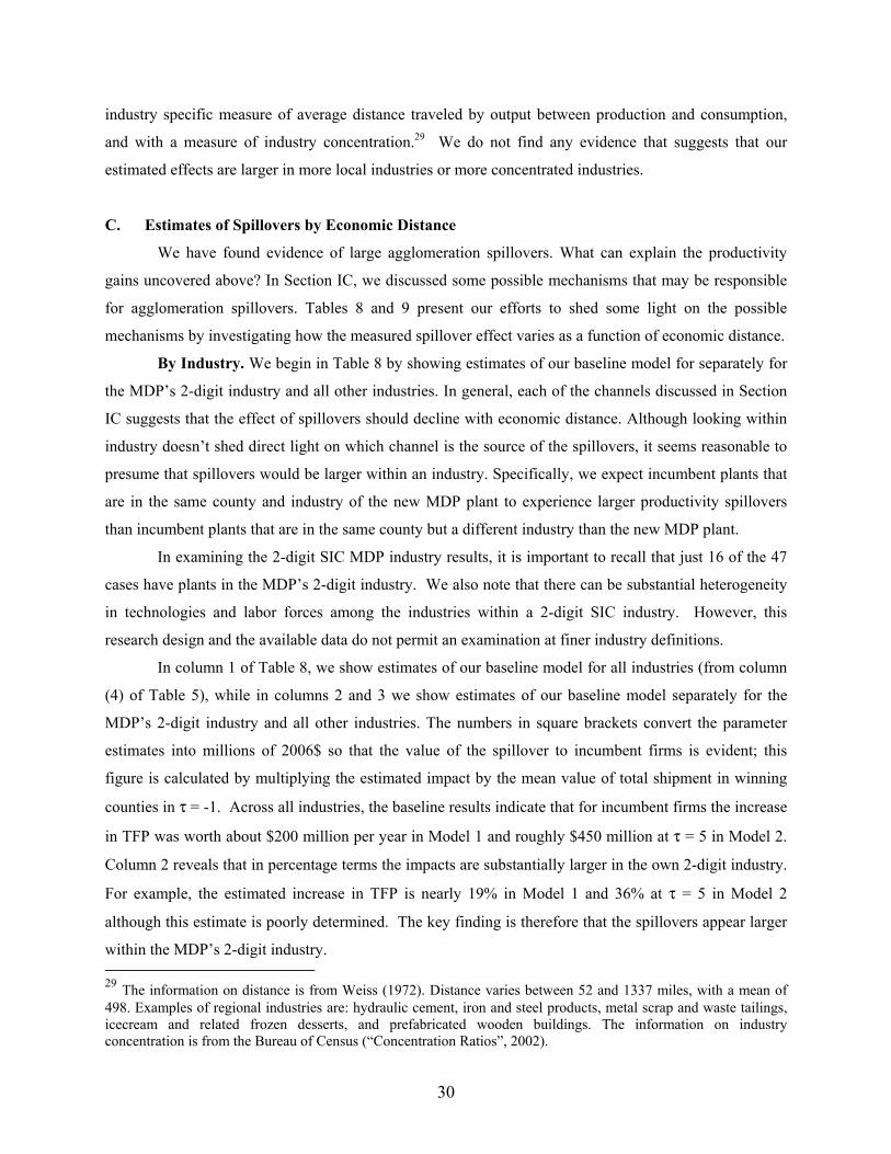
30
industry specific measure of average distance traveled by output between production and consumption,
and with a measure of industry concentration.29 We do not find any evidence that suggests that our
estimated effects are larger in more local industries or more concentrated industries.
C. Estimates of Spillovers by Economic Distance
We have found evidence of large agglomeration spillovers. What can explain the productivity
gains uncovered above? In Section IC, we discussed some possible mechanisms that may be responsible
for agglomeration spillovers. Tables 8 and 9 present our efforts to shed some light on the possible
mechanisms by investigating how the measured spillover effect varies as a function of economic distance.
By Industry. We begin in Table 8 by showing estimates of our baseline model for separately for
the MDP�s 2-digit industry and all other industries. In general, each of the channels discussed in Section
IC suggests that the effect of spillovers should decline with economic distance. Although looking within
industry doesn�t shed direct light on which channel is the source of the spillovers, it seems reasonable to
presume that spillovers would be larger within an industry. Specifically, we expect incumbent plants that
are in the same county and industry of the new MDP plant to experience larger productivity spillovers
than incumbent plants that are in the same county but a different industry than the new MDP plant.
In examining the 2-digit SIC MDP industry results, it is important to recall that just 16 of the 47
cases have plants in the MDP�s 2-digit industry. We also note that there can be substantial heterogeneity
in technologies and labor forces among the industries within a 2-digit SIC industry. However, this
research design and the available data do not permit an examination at finer industry definitions.
In column 1 of Table 8, we show estimates of our baseline model for all industries (from column
(4) of Table 5), while in columns 2 and 3 we show estimates of our baseline model separately for the
MDP�s 2-digit industry and all other industries. The numbers in square brackets convert the parameter
estimates into millions of 2006$ so that the value of the spillover to incumbent firms is evident; this
figure is calculated by multiplying the estimated impact by the mean value of total shipment in winning
counties in τ = -1. Across all industries, the baseline results indicate that for incumbent firms the increase
in TFP was worth about $200 million per year in Model 1 and roughly $450 million at τ = 5 in Model 2.
Column 2 reveals that in percentage terms the impacts are substantially larger in the own 2-digit industry.
For example, the estimated increase in TFP is nearly 19% in Model 1 and 36% at τ = 5 in Model 2
although this estimate is poorly determined. The key finding is therefore that the spillovers appear larger
within the MDP�s 2-digit industry. 29 The information on distance is from Weiss (1972). Distance varies between 52 and 1337 miles, with a mean of 498. Examples of regional industries are: hydraulic cement, iron and steel products, metal scrap and waste tailings, icecream and related frozen desserts, and prefabricated wooden buildings. The information on industry concentration is from the Bureau of Census (�Concentration Ratios�, 2002).

31
To graphically appreciate the effect by industry, Figures 3 and 4 provide 2-digit MDP industry
and other industry analogues to Figure 1. Importantly, there isn�t evidence of differential trends in years
before the MDP�s opening and statistical tests confirm this visual impression. The 2-digit MDP industry
estimates are noisy due to the small sample size, which was also evident in the statistical results. Just as
in Figure 1, the estimated impact reflects the continuation of a downward trend in TFP in losing counties
and a cessation of the downward trend in winning counties.
By Explicit Measure of Economic Distance. In Table 9 we turn to more articulated measures of
economic distance. We estimate models similar to the one in equation (11), but we now include an
explicit measure of economic proximity between the relevant plant and the new MDP plant, as well as the
interaction between winning county status and economic proximity. The coefficient of interest is the one
on the interaction. We have four alternative measures of economic proximity. The idea is that we want to
see which measures of economic distance are associated with large spillover effects. For example, finding
that the interaction with the measure of proximity based on workers transitions is large, may suggest that
spillovers occur through the flow of workers across firms, possibly because workers brings with
themselves new ways of organizing production or information on new technologies learned with the
previous employer. On the other hand, finding that the interaction with proximity as measured by input-
output tables is large, may suggest that spillovers occur through the exchange of local goods and services.
The first 6 columns in Table 9 report on the interaction of the parameter of interest from Model
1, that is (1(Winner) * 1(τ >= 0))pjt, with standardized versions of the six industry linkage variables.
These six specifications put these interactions in one at a time, while columns (7) and (8) conduct �horse
races� that include all but the labor pooling variable and all of them, respectively. Throughout this
analysis, the variables are standardized to have a mean of zero and standard deviation of one to ease the
interpretation of the associated parameters.
The specifications that put these interactions in one at a time are supportive of nation that
spillovers are associated with flow of workers and with technological proximity. For example, column
(1) suggests that a one standard deviation increase in the CPS Worker Transitions variable between
incumbent plants� industry and the MDP�s industry is associated with a 7.5% increase in the spillover.
This measure tends to be especially high within 2-digit industries, so this finding was foreshadowed by
the own 2-digit results in Table 2. Two of the three measures of intellectual or technological linkages
indicate statistically meaningful increases in the spillover. Columns (5) and (6) provide little support for
the flow of goods and services in determining the magnitude of spillovers.
In the column (8) specification, the labor flow, the citation pattern, and the technology input
interactions all remain positive but now would be judged to be statistically insignificant. The interactions
with proximity to customers and suppliers are now both negative. Overall, this analysis provides some

32
support for the notion that spillovers occurs between firms that share workers and between firms that use
similar technologies. In terms of Section IC, this evidence is consistent with intellectual externalities, to
the extent that they are embodied in workers who move from firm to firm, and to the extent that they
occur among firms that use technologies that are reasonably similar. Table 9 seems less consistent with
the hypothesis that agglomeration occurs because of proximity to customers and suppliers. However, we
caution against definitive conclusions based on Table 9. The tests presented are very indirect, and it is
impossible to rule out alternative hypotheses with certainty.
D. Profits
In Tables 5, 6 and 7 we have uncovered significant productivity gains for incumbent
establishments following the opening of a new establishment. These productivity gains appear to be
economically sizable. A MDP plant opening is associated with a 13% increase in TFP five years later.
This effect is even larger for incumbent plants that are in the same 2-digit industry of the new plant, and
for plants that tend to share technology and labor force.
Do these increases in productivity translate into equally large increases in profits? Not
necessarily. Equation (3) in Section I clarifies that the effect on profits is likely to be smaller than the
effect on productivity. The reason is obvious from in equation (3). The effect on profits can be
decomposed in two parts. The first term, (δf /δA δA/δN), is the productivity gain uncovered in Tables 5,
6 and 7. The second term, -[ δw/δN L + δq/δN T], is the effect of higher labor and land costs induced by
the increases in input demand generated by the opening of new plant. This second term is negative, as
higher inputs costs lower profits.
While we believe that the increase in profits is smaller than the measured gain in TFP, we can not
conclusively measure the effect on profits, because we do not observe the quality-adjusted price of all
inputs. Instead, we provide some pieces of evidence that might help in characterizing the effect on profits.
In column 1 of Table 10 we show how wages change in response to a MDP opening. Specifically,
the dependent variable is log wage and controls include dummies for age*year, age-squared*year,
education*year, sex*race*Hispanic*citizen, and case fixed effects. The entry is the county-level
difference in difference estimate for winning a MDP, based on Census of Population data.30 We use
Census data, instead of labor costs reported in the Census of Manufacturers, because the latter only report
30 The pre-period is defined as the most recent census before the MDP opening. The post-period is defined as the most recent census 3 or more years after the MDP opening. Thus, the sample years are 1 � 10 years before the MDP opening and 3 � 12 years after the MDP opening. The sample is limited to individuals who worked last year, worked more than 26 weeks, usually work more than 20 hours per week, are not in school, are at work, and who work for wages in the private sector. One important limitation of Census data is that they lack exact county identifier. Census provides instead PUMA�s, which in rural areas can include several counties. This introduces significant measurement error, which is partly responsible for the imprecision of the estimate.

33
aggregate wage bill for production and non-production workers, and therefore does not allow to properly
account for changes in the quality of labor. The estimate indicates that after adjusting for observable
heterogeneity, labor cost increases by 2.6% in counties that receive a new MDP plant. This effect appears
quantitatively sizable. As discussed in Section I, it is consistent with an upward sloping labor supply
curve, probably due to imperfect mobility of labor, at least in the short run. While not explicitly included
in the model, any intermediate input or service that is locally purchased might also experience upward
price pressure, at least in the short run. Unfortunately, the existing data do not allow us to measure this
additional effect.
In Panel 2 of Table 10 we seek to determine whether the opening of an MDP plant is associated
with entry of new establishments or exit of incumbent establishments. The finding of positive net entry
may indicate that the plant opening is associated with an increase in profits, at least in the manufacturing
sector. In terms of equation (3), it would indicate that the first term is larger than the second term. Of
course, this estimate refers only to manufacturing firms, and therefore do not tell us about how profits in
other parts of the local economy may be affected. However, we note that the manufacturing sector should
be the sector most sensitive to increased in local costs generated by the plant opening. The reason is that
manufacturing produces traded goods, and therefore can not raise prices to pass cost increases to
consumers. By contrast, local services can raise prices when the cost of inputs increases. This implies that
the finding of some positive net entry in the manufacturing sector may indicate an increase in profits in
other sectors as well.
The dependent variables in column 2 and 3 are the log of number of establishments and the log of
total manufacturing output in the county, respectively. Controls include case effects, county, and year
fixed effects. Entries are the county-level diff in diff estimates for winning a MDP, based on data from the
Census of Manufacturers.31 Column 2 and 3 indicate that the opening of a new plant may be associated
with positive net entry, although the estimates are too imprecise to draw firm conclusions.
Finally, we have also attempted to estimate accounting profits directly. Specifically, we have run
regression where the dependent variable is value of shipments minus the total wage bill, the cost of
materials and the user cost of capital based on BLS capital rental rates. A mean shift model of the type of
Model 1 in Panel A of Table 6 yields a coefficient equal to .1187 (.0773), not very different from the
equivalent effect on TFP. A regression similar to Model 2 in Panel A of Table 6 yields a 5-years effect
equal to .0952 (.0874). However, we note that due to data limitations, this accounting measure of profits
is not fully satisfactory. First, it does not include the value of intermediate local goods or services. As
31 Because data is available every 5 years, depending on the Census year relative to the MDP opening, the sample years are 1 � 5 years before the MDP opening and 4 � 8 years after the MDP opening. Thus, each MDP opening is associated with one earlier date and one later date. Models are weighted by the number of plants in the county in years -6 to -10 and column 4 is weighted by the county�s total manufacturing output in years -6 to -10.

34
discussed above, their price is likely to vary in response to a MDP plant opening. Second, it requires
assumptions on the interest rate to determine the user cost of capital. Third, as for the entry and exit
analysis above, these estimates refer only to manufacturing firms, and therefore do not tell us about
profits in other parts of the local economy. For these reasons, we caution against reading too much into
this specific result.
VI. Conclusion
Estimation of agglomeration spillovers is challenging. Localities differ in so many dimensions
that it is difficult to draw firm conclusions on the existence and magnitude of spillovers simply based on
the observed agglomeration of economic activity. In our sample, naïve estimates that control only for
observable characteristics fail to detect any spillover effects. By contrast, when we use a more credible
identification strategy based on Million Dollar Plant openings, we find evidence of the existence of
substantial agglomeration spillovers.
Following the opening of a new plant in a county, incumbent plants appear to be able to produce
more with the same inputs. Specifically, the opening of a new plant is associated on average with 13%
increase in incumbent plants total factor productivity five years later. This effect is even larger for pair of
industries that are linked by intense flows of workers mobility and pair of industries that employ similar
technologies.
While these productivity effects are large, they do not necessarily translate into higher profits.
After the opening of the new plant, the incumbent plants as well as non-manufacturing firms in the same
county face more intense competition for labor and other local inputs that are inelastically supplied.
Indeed, standard wage regressions suggest that the price of quality-adjusted labor does in fact increase in
affected counties. While we can not exactly quantify the effect on profits, we do find some evidence of
increased entry in the manufacturing sector following the opening of a new plant.
Overall, our estimates support the notion that firms agglomerate in certain localities at least in
part because they are more productive for being close to other firms. Moreover, our analysis lends some
support for the notion that such spillovers are driven by intellectual externalities, to the extent that they
are embodied in workers who move from firm to firm, and occur among firms that use technologies that
are reasonably similar. Our evidence is less consistent with the hypothesis that agglomeration spillovers
occurs because of proximity to customers and suppliers.

35
Bibliography
Acemoglu, D. (1996), 'A microfundation for social increasing returns in human capital accumulation', Quarterly Journal of Economics pp. 779-804. Audretsch David and Feldman, Maryann �R&D Spillovers and the Geography of Innovation and Production� American Economic Review 86 pp 630-640 (1996) Audretsch David and Feldman, Maryann �Knowledge Spillovers and the Geography of Innovation� in Handbook of Urban and Regional Economics, Henderson and Thisse (Editors), North-Holland (2004) Nick Bloom, Mark Schankerman, John Van Reenen �Identifying Technology Spillovers and Product Market Rivalry� NBER WP 13060 Branstetter, L. (2001), 'Are knowledge spillovers international or international in scope? microeconomic evidence from us and Japan', Journal of International Economics 53, 53-79. Card, Hallock and Moretti, 2007, �The Geography of Giving: The Effect of Corporate Headquarters on Local Charities� Davis, James, and Vernon Henderson, 2004. �The Agglomeration of Headquarters," Unpublished working paper, Brown University Department of Economics. Dumais, Guy, Ellison, Glenn and Glaeser, Edward L. (2002): .Geographic Concentration as a Dynamic Process,.Review of Economics and Statistics, 84, 193.204. Duranton and Puga �Micro-Foundations of Urban Agglomeration Economies� in Handbook of Urban and Regional Economics, Henderson and Thisse (Editors), North-Holland (2004) Ellison, Glenn and Glaeser, Edward L. (1997): .Geographic Concentration in U.S. Manufacturing Industries: A Dartboard Approach, .Journal of Political Economy, 105, 889.927. Ellison, Glaeser and Kerr �What Causes Industry Agglomeration? Evidence from Coagglomeration Patterns�, NBER WP 13068 (2007). Glaeser, E. L. (1999), 'Learning in cities', Journal of Urban Economics 46(2), 254-77. Glaeser E.L. and J. E. Kohlhase, �Cities, Regions and the Decline of Transport Costs�, Papers in Regional Science, 83, 2003 Glaeser, E. L �The Economics of Location-Based Tax Incentives�, Harvard University, 2001 Greenstone and Moretti, "Bidding for Industrial Plants: Does Winning a 'Million Dollar Plant' Increase Welfare?" mimeo (2004). Grossman and Helpman �Innovation and Growth in the Global Economy�, MIT Press (1991)

36
Henderson, J.V. and Black, D. "The Theory of Urban Growth," Journal of Political Economy, 1999, 107, 252-284 Henderson, J.V. �"Urban Scale Economies," Sage Handbook of Urban Studies, R. Paddison (ed.), 2001. Henderson, J.V., 'Marshall's scale economies', Journal of Urban Economics (2003) Jaffe, A. B. (1986), 'Technological opportunities and spillovers of r&d: Evidence from firm's patents, profit and market value', American Economic Review 76, 984~1001. Jaffe, A., Trajtenberg, M. and Henderson, R. (1993), 'Geographic localization of knowledge spillovers as evidenced by patent citation', Quarterly Journal of Economics 108(3), 577- 598. Jaffe, A., Trajtenberg, M. and Henderson, R. (2002), Patents, Citations and Innovations, MIT Press. Jaffe, Adam, Trajtenberg (2000): .Knowledge Spillovers and Patent Citations: Evidence from a Survey of Inventors�, Papers and Proceedings, American Economic Review, 90, 215.218. Jovanovic, B. and Rob, R. (1989), 'The growth and diffusion of knowledge', Review of Economic Studies 56(4), 569-582. Krugman, Paul (1991): Geography and Trade. Cambridge, MA: MIT Press. Krugman, Paul �Increasing Returns and Economic Geography�, Journal of Political Economy, 99 pp. 483-499, (1991) James Levinsohn and Amil Petrin, "Estimating Production Functions Using Inputs to Control for Unobservables," Review of Economic Studies , April, 2003, Vol. 70(2), No. 243, pp. 317-342 Lucas, R. E. (1988), 'On the mechanics of economic development', Journal of Monetary Economics 22, 3-42. Marshall, A. (1890), Principles of Economics, Macmillan. McGahan, A. and Silverman, B. (2001), 'How does innovative activity change as industries mature?', International Journal of Industrial Organization 19. Moretti, E., 'Estimating the external return to higher education: Evidence from cross-sectional and longitudinal data', Journal of Econometrics (2004a)
Moretti, E. �"Workers' Education, Spillovers and Productivity: Evidence from Plant-Level Production Functions" American Economic Review 94(3), (2004b)

37
Moretti, E. "Human Capital Externalities in Cities" in Handbook of Urban and Regional Economics, Henderson and Thisse (Editors), North-Holland (2004c) Mowery, D. and Ziedonis, A. (2001), 'The geographic reach of market and non-market channels of technology transfer: Comparing citations and licenses of university patents', NBER Working Paper 8568 .
Olley Steve and Ariel Pakes (1996), �The Dynamics of Productivity in the Telecommunications Equipment Industry� Econometrica, vol. 64, no. 6, pp. 1263-98. Ottaviano and Thisse �Agglomeration and Economic Geography�, in Handbook of Urban and Regional Economics, Henderson and Thisse (Editors), North-Holland (2004) Petrongolo and Pissarides, �Scale Effects in Markets with Search� Economic Journal 116 21-44 (2005). Rauch, J. E. (1993), 'Productivity gains from geographic concentration of human capital: Evidence from the cities', Journal of Urban Economics 34, 380-400. Roback, J. (1982), 'Wages, rents and the quality of life', Journal of Political Economy 90(6), 1257-1278. Roback, J. (1988), 'Wages, rents and amenities: Differences among workers and regions', Economic Inquiry 26(1), 23-41. Rosenthal and Stange, �The Determinants of Agglomeration�, Journal of Urban Economics 50, 191-229, (2001). Rosenthal and Stange �Evidence on the Nature and Sources of Agglomeration� in Handbook of Urban and Regional Economics, Henderson and Thisse (Editors), North-Holland (2004) Saxenian, Anna Lee (1994): Regional Advantage: Culture and Competition in Silicon Valley and Route 128. Cambridge, MA: Harvard University Press. Syverson, Chad �Market Structure and Productivity: A Concrete Example," Journal of Political Economy, December 2004 Syverson, Chad "Product Substitutability and Productivity Dispersion," Review of Economics and Statistics, May 2004 Weiss, L. W. (1972), 'The geographic size of markets in manufacturing', The Review of Economics and Statistics 54. Zucker, L. G., Darby, M. R. and Brewer, M. B. (1998), 'Intellectual human capital and the birth of US biotechnology enterprises', American Economic Review 88(1), 290-306.

38
Figure 1: The Effect of a �Million Dollar Plant� Opening on TFP of All Manufacturing Plants in Winner and Loser Counties.
All Industries: Winners Vs. Losers
-0.15
-0.1
-0.05
0
0.05
0.1
-7 -6 -5 -4 -3 -2 -1 0 1 2 3 4 5
Year, relative to opening
Winning Counties Losing Counties
Difference: Winners � Losers
-0.05
0
0.05
0.1
-7 -6 -5 -4 -3 -2 -1 0 1 2 3 4 5
Year, relative to opening
Notes: These figures accompany Table 6, Column 1, Panel A (All Industries).

39
Figure 2. Distribution of Case-Specific Mean Shift Effects from the Opening of a �Million Dollar Plant�
-0.5
-0.4
-0.3
-0.2
-0.1
0
0.1
0.2
0.3
0.4
0.5
1 45
Notes: The Figure reports results from a version of Model 1 that estimates the parameter θ1 for each of the 47 MDP cases. The figure reports only 45 estimates because two cases were dropped for Census confidentiality reasons.

40
Figure 3: The Effect of a �Million Dollar Plant� Opening on TFP of Manufacturing Plants in MDP�s 2-Digit Industry in Winner and Loser Counties.
2-digit M$P Industry: Winners Vs. Losers
-0.2
-0.1
0
0.1
0.2
-7 -6 -5 -4 -3 -2 -1 0 1 2 3 4 5
Year, relative to opening
Winning Counties Losing Counties
Difference (Winners � Losers)
-0.3
-0.2
-0.1
0
0.1
0.2
0.3
-7 -6 -5 -4 -3 -2 -1 0 1 2 3 4 5
Year, relative to opening
Notes: These figures accompany Table 6, Column 1, Panel B (2-digit M$P Industry).
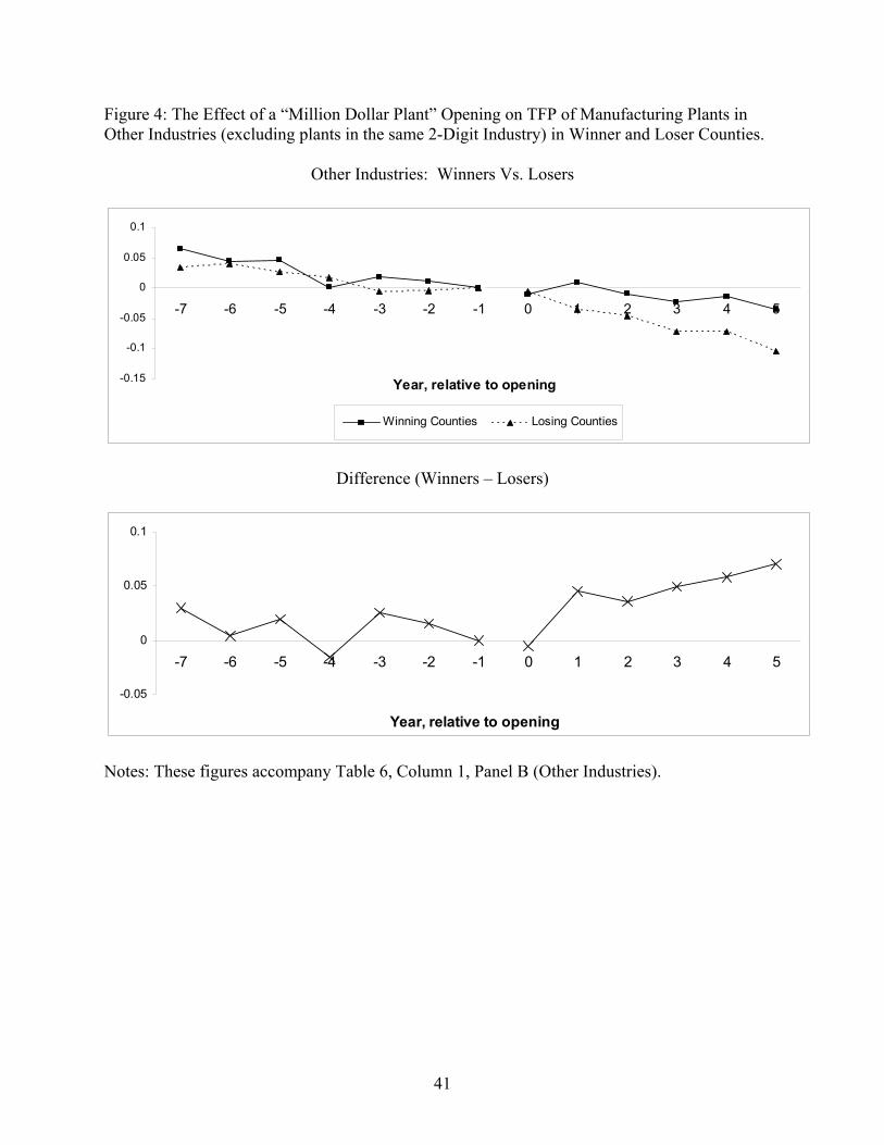
41
Figure 4: The Effect of a �Million Dollar Plant� Opening on TFP of Manufacturing Plants in Other Industries (excluding plants in the same 2-Digit Industry) in Winner and Loser Counties.
Other Industries: Winners Vs. Losers
-0.15
-0.1
-0.05
0
0.05
0.1
-7 -6 -5 -4 -3 -2 -1 0 1 2 3 4 5
Year, relative to opening
Winning Counties Losing Counties
Difference (Winners � Losers)
-0.05
0
0.05
0.1
-7 -6 -5 -4 -3 -2 -1 0 1 2 3 4 5
Year, relative to opening
Notes: These figures accompany Table 6, Column 1, Panel B (Other Industries).

42
Table 1. The �Million Dollar Plant� Sample
(1) MDP Magazine Openings 82 Sample MDP Openings¹:
Across All Industries 47 Within Same 2-digit SIC 16
Across All Industries:
Number of Loser Counties per Winner County: 1 31 2+ 16 Reported Year � Matched Year: ² -2 to -1 20 0 15 1 to 3 12 Reported Year of MDP Location: 1981 � 1985 11 1986 � 1989 18 1990 � 1993 18
MDP Characteristics, 5 years after opening:³ Output ($1000) 452801 (901690)
0.086 Output, relative to county output 1 year prior (0.109)
Hours of Labor (1000) 2986 (6789)
¹ Million Dollar Plant openings that were matched to the Census data and for which there were incumbent plants in both winning and losing counties that are observed in each of the eight years prior to the opening date (the opening date is defined as the earliest of the magazine reported year and the year observed in the SSEL.) This sample is then restricted to include matches for which there were incumbent plants in the Million Dollar Plant�s 2-digit SIC in both locations. ² Only a few of these differences are 3. ³ Of the original 47 cases, these statistics represent 28 cases. A few very large outlier plants were dropped so that the mean would be more representative of the entire distribution (those dropped had output greater than half of their county�s previous output and sometimes much more). Of the remaining cases: most SSEL matches were found in the ASM or CMF but not exactly 5 years after the opening date; a couple SSEL matches in the 2xxx-3xxx SICs were never found in the ASM or CMF; and a couple SSEL matches not found were in the 4xxx SICs. The MDP characteristics are similar for cases identifying the effect within same 2-digit SIC. All monetary amounts are in 2006 US dollars.
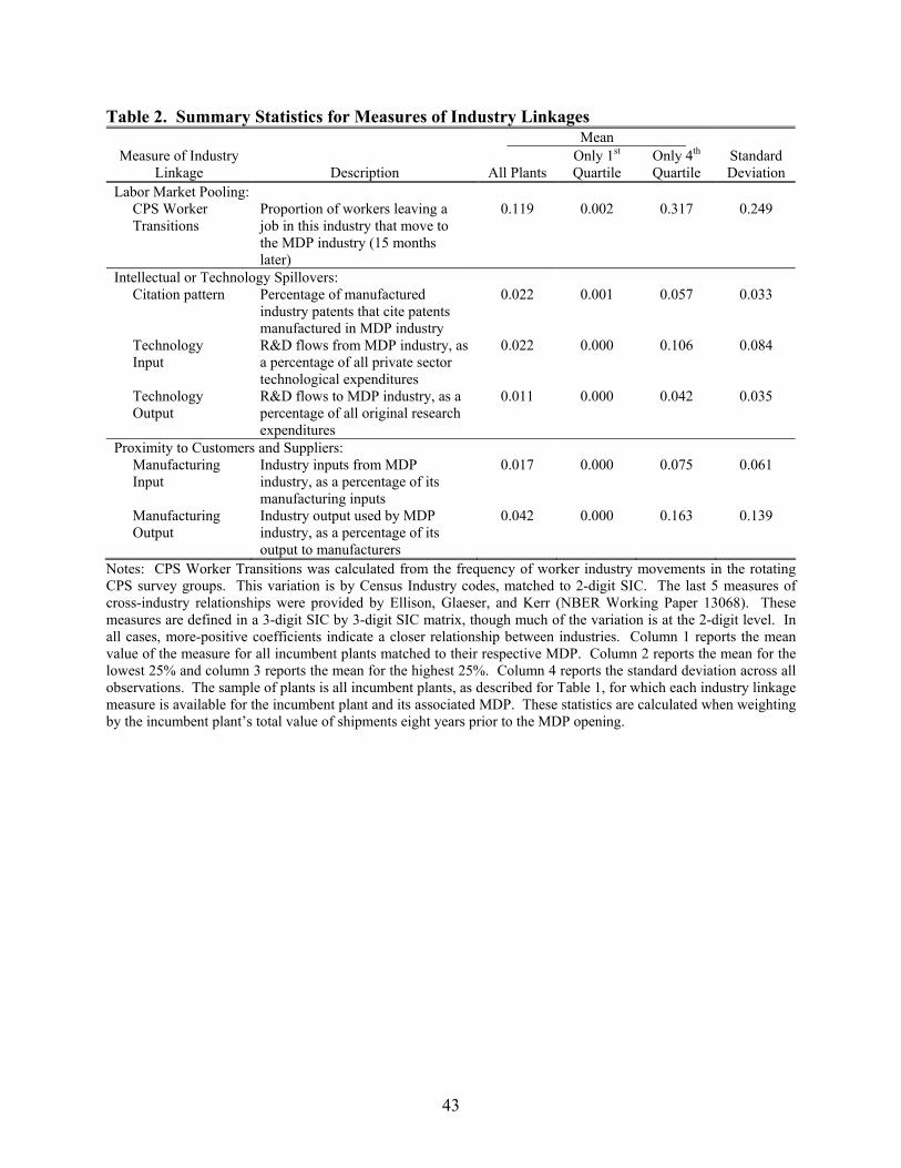
43
Table 2. Summary Statistics for Measures of Industry Linkages Mean
Measure of Industry Linkage Description All Plants
Only 1st Quartile
Only 4th Quartile
Standard Deviation
Labor Market Pooling: CPS Worker Transitions
Proportion of workers leaving a job in this industry that move to the MDP industry (15 months later)
0.119 0.002 0.317 0.249
Intellectual or Technology Spillovers: Citation pattern Percentage of manufactured
industry patents that cite patents manufactured in MDP industry
0.022 0.001 0.057 0.033
Technology Input
R&D flows from MDP industry, as a percentage of all private sector technological expenditures
0.022 0.000 0.106 0.084
Technology Output
R&D flows to MDP industry, as a percentage of all original research expenditures
0.011 0.000 0.042 0.035
Proximity to Customers and Suppliers: Manufacturing Input
Industry inputs from MDP industry, as a percentage of its manufacturing inputs
0.017 0.000 0.075 0.061
Manufacturing Output
Industry output used by MDP industry, as a percentage of its output to manufacturers
0.042 0.000 0.163 0.139
Notes: CPS Worker Transitions was calculated from the frequency of worker industry movements in the rotating CPS survey groups. This variation is by Census Industry codes, matched to 2-digit SIC. The last 5 measures of cross-industry relationships were provided by Ellison, Glaeser, and Kerr (NBER Working Paper 13068). These measures are defined in a 3-digit SIC by 3-digit SIC matrix, though much of the variation is at the 2-digit level. In all cases, more-positive coefficients indicate a closer relationship between industries. Column 1 reports the mean value of the measure for all incumbent plants matched to their respective MDP. Column 2 reports the mean for the lowest 25% and column 3 reports the mean for the highest 25%. Column 4 reports the standard deviation across all observations. The sample of plants is all incumbent plants, as described for Table 1, for which each industry linkage measure is available for the incumbent plant and its associated MDP. These statistics are calculated when weighting by the incumbent plant�s total value of shipments eight years prior to the MDP opening.

44
Tab
le 3
. C
ount
y &
Pla
nt C
hara
cter
istic
s by
Win
ner
Stat
us, O
ne Y
ear
Prio
r to
a �
Mill
ion
Dol
lar
Plan
t� O
peni
ng
A
ll Pl
ants
W
ithin
Sam
e In
dust
ry (2
-dig
it SI
C)
W
inni
ng
Cou
ntie
s Lo
sing
C
ount
ies
All
US
Cou
ntie
s (1
) � (2
) t-s
tat
(1) �
(3)
t-sta
t W
inni
ng
Cou
ntie
s Lo
sing
C
ount
ies
All
US
Cou
ntie
s (6
) � (7
) t-s
tat
(6) �
(8)
t-sta
t
(1)
(2)
(3)
(4)
(5)
(6)
(7)
(8)
(9)
(10)
#
of C
ount
ies
47
73
16
19
Cou
nty
Cha
ract
eris
tics:
Tota
l Per
-cap
ita E
arni
ngs (
$)
1741
8 20
628
1125
9 -2
.05
5.79
20
230
2052
8 11
378
-0.1
1 4.
62
%
Cha
nge,
ove
r las
t 6 y
ears
0.
074
0.09
6 0.
037
-0.8
1 1.
67
0.07
6 0.
089
0.05
7 -0
.28
0.57
Po
pula
tion
3227
45
4478
76
8238
1 -1
.61
4.33
35
7955
50
4342
83
430
-1.1
7 3.
26
%
Cha
nge,
ove
r las
t 6 y
ears
0.
102
0.05
1 0.
036
2.06
3.
22
0.07
0 0.
032
0.03
1 1.
18
1.63
Em
ploy
men
t-Pop
ulat
ion
ratio
0.
535
0.57
9 0.
461
-1.4
1 3.
49
0.60
2 0.
569
0.46
7 0.
64
3.63
Cha
nge,
ove
r las
t 6 y
ears
0.
041
0.04
7 0.
023
-0.6
8 2.
54
0.04
5 0.
038
0.02
8 0.
39
1.57
Man
ufac
turin
g La
bor S
hare
0.
314
0.25
1 0.
252
2.35
3.
12
0.29
6 0.
227
0.25
1 1.
60
1.17
Cha
nge,
ove
r las
t 6 y
ears
-0
.014
-0
.031
-0
.008
1.
52
-0.6
4 -0
.030
-0
.040
-0
.007
0.
87
-3.1
7
# of
Sam
ple
Plan
ts
18.8
25
.6
7.98
-1
.35
3.02
2.
75
3.92
2.
38
-1.1
4 0.
70
Plan
t Cha
ract
eris
tics:
19
0039
18
1454
12
3187
0.
25
2.14
21
7950
17
8958
13
2570
0.
41
1.25
O
utpu
t ($1
000)
0.
082
0.08
2 0.
118
0.01
-0
.97
-0.0
61
0.17
7 0.
182
-1.2
3 -3
.38
% C
hang
e, o
ver l
ast 6
yea
rs
1508
11
68
877
1.52
2.
43
1738
11
98
1050
0.
92
1.33
H
ours
of l
abor
(100
0)
0.12
2 0.
081
0.11
5 0.
81
0.14
0.
160
0.02
3 0.
144
0.85
0.
13
% C
hang
e, o
ver l
ast 6
yea
rs
Not
es:
For e
ach
case
to b
e w
eigh
ted
equa
lly, c
ount
ies
are
wei
ghte
d by
the
inve
rse
of th
eir n
umbe
r per
-cas
e. S
imila
rly, p
lant
s ar
e w
eigh
ted
by th
e in
vers
e of
thei
r nu
mbe
r per
-cou
nty
mul
tiplie
d by
the
inve
rse
of th
e nu
mbe
r of c
ount
ies
per-
case
. Th
e sa
mpl
e in
clud
es a
ll pl
ants
repo
rting
dat
a in
the
ASM
for e
ach
year
bet
wee
n th
e M
DP
open
ing
and
eigh
t yea
rs p
rior.
Exc
lude
d ar
e al
l pla
nts
owne
d by
the
firm
ope
ning
a M
DP.
Als
o ex
clud
ed a
re a
ll pl
ants
from
two
unco
mm
on 2
-dig
it SI
C
valu
es s
o th
at s
ubse
quen
tly e
stim
ated
clu
ster
ed v
aria
nce
mat
rices
wou
ld a
lway
s be
pos
itive
def
inite
. Th
e sa
mpl
e of
all
US
coun
ties
excl
udes
win
ning
cou
ntie
s an
d co
untie
s w
ith n
o m
anuf
actu
ring
plan
t rep
ortin
g da
ta in
the
ASM
for n
ine
cons
ecut
ive
year
s. T
hese
oth
er U
S co
untie
s ar
e gi
ven
equa
l wei
ght w
ithin
yea
rs a
nd a
re
wei
ghte
d ac
ross
yea
rs to
repr
esen
t the
yea
rs o
f MD
P op
enin
gs.
Rep
orte
d t-s
tatis
tics a
re c
alcu
late
d fr
om st
anda
rd e
rror
s clu
ster
ed a
t the
cou
nty
leve
l. A
ll m
onet
ary
amou
nts a
re in
200
6 U
S do
llars
.
45
Table 4. Incumbent Plant Productivity, Relative to the Year of a MDP Opening Relative Year In Winning
Counties In Losing Counties
Difference (1) � (2)
(1) (2) (3) τ = -7 0.067 0.040 0.027 0.058 0.053 0.032 τ = -6 0.047 0.028 0.018 0.044 0.046 0.023 τ = -5 0.041 0.021 0.020 0.036 0.040 0.025 τ = -4 -0.003 0.012 -0.015 0.030 0.030 0.024 τ = -3 0.011 -0.013 0.024 0.022 0.022 0.021 τ = -2 -0.003 0.001 -0.005 0.027 0.011 0.028 τ = -1 0 0 0 τ = 0 0.013 -0.010 0.023 0.018 0.011 0.019 τ = 1 0.023 -0.028 0.051 0.026 0.024 0.023 τ = 2 0.004 -0.046 0.050 0.036 0.046 0.033 τ = 3 0.003 -0.073 0.076 0.047 0.057 0.043 τ = 4 0.004 -0.072 0.076 0.053 0.062 0.033 τ = 5 -0.023 -0.100 0.077 0.069 0.067 0.035 R-squared 0.9861 Observations 28732
Notes: Standard errors are clustered at the county level. Columns 1 and 2 report coefficients from the same regression: the natural log of output is regressed on the natural log of inputs (all worker hours, building capital, machinery capital, materials), year x 2-digit SIC fixed effects, plant fixed effects, case fixed effects, and the reported dummy variables for whether the plant is in a winning or losing county in each year relative to the MDP opening. When a plant is a winner or loser more than once, it receives a dummy variable for each incident. Plant-year observations are weighted by the plant�s total value of shipments eight years prior to the MDP opening. Data on plants in all cases is only available 8 years prior to the MDP opening and 5 years after. Capital stocks were calculated using the permanent inventory method from early book values and subsequent investment. The sample of incumbent plants is the same as in columns 1 � 2 of Table 3.
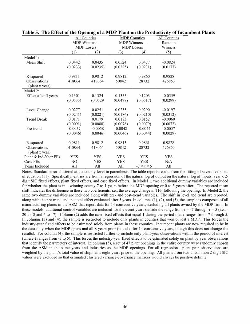
46
Table 5. The Effect of the Opening of a MDP Plant on the Productivity of Incumbent Plants All Counties MDP Counties All Counties MDP Winners �
MDP Losers MDP Winners �
MDP Losers Random Winners
(1) (2) (3) (4) (5) Model 1: Mean Shift 0.0442 0.0435 0.0524 0.0477 -0.0824 (0.0233) (0.0235) (0.0225) (0.0231) (0.0177) R-squared 0.9811 0.9812 0.9812 0.9860 0.9828 Observations (plant x year)
418064 418064 50842 28732 426853
Model 2: Effect after 5 years 0.1301 0.1324 0.1355 0.1203 -0.0559 (0.0533) (0.0529 (0.0477) (0.0517) (0.0299) Level Change 0.0277 0.0251 0.0255 0.0290 -0.0197 (0.0241) (0.0221) (0.0186) (0.0210) (0.0312) Trend Break 0.0171 0.0179 0.0183 0.0152 -0.0060 (0.0091) (0.0088) (0.0078) (0.0079) (0.0072) Pre-trend -0.0057 -0.0058 -0.0048 -0.0044 -0.0057 (0.0046) (0.0046) (0.0046) (0.0044) (0.0029) R-squared 0.9811 0.9812 0.9813 0.9861 0.9828
418064 418064 50842 28732 426853 Observations (plant x year) Plant & Ind-Year FEs YES YES YES YES YES Case FEs NO YES YES YES N/A Years Included All All All -7 ≤ τ ≤ 5 All
Notes: Standard error clustered at the county level in parenthesis. The table reports results from the fitting of several versions of equation (11). Specifically, entries are from a regression of the natural log of output on the natural log of inputs, year x 2-digit SIC fixed effects, plant fixed effects, and case fixed effects. In Model 1, two additional dummy variables are included for whether the plant is in a winning county 7 to 1 years before the MDP opening or 0 to 5 years after. The reported mean shift indicates the difference in these two coefficients, i.e., the average change in TFP following the opening. In Model 2, the same two dummy variables are included along with pre- and post-trend variables. The shift in level and trend are reported, along with the pre-trend and the total effect evaluated after 5 years. In columns (1), (2), and (5), the sample is composed of all manufacturing plants in the ASM that report data for 14 consecutive years, excluding all plants owned by the MDP firm. In these models, additional control variables are included for the event years outside the range from τ = -7 through τ = 5 (i.e., -20 to -8 and 6 to 17). Column (2) adds the case fixed effects that equal 1 during the period that τ ranges from -7 through 5. In columns (3) and (4), the sample is restricted to include only plants in counties that won or lost a MDP. This forces the industry-year fixed effects to be estimated solely from plants in these counties. Incumbent plants are now required to be in the data only when the MDP opens and all 8 years prior (not also for 14 consecutive years, though this does not change the results). For column (4), the sample is restricted further to include only plant-year observations within the period of interest (where τ ranges from -7 to 5). This forces the industry-year fixed effects to be estimated solely on plant by year observations that identify the parameters of interest. In column (5), a set of 47 plant openings in the entire country were randomly chosen from the ASM in the same years and industries as the MDP openings. For all regressions, plant-year observations are weighted by the plant�s total value of shipments eight years prior to the opening. All plants from two uncommon 2-digit SIC values were excluded so that estimated clustered variance-covariance matrices would always be positive definite.

47
Tab
le 6
The
Eff
ect o
f the
Ope
ning
of a
MD
P Pl
ant o
n th
e Pr
oduc
tivity
of I
ncum
bent
Pla
nts.
Rob
ustn
ess t
o D
iffer
ent
Spec
ifica
tions
Bas
elin
e sp
ecifi
catio
n Tr
ansl
og
func
tiona
l fo
rm
Inpu
t -
indu
stry
in
tera
ctio
ns
Inpu
t-w
inne
r, in
put-p
ost
Reg
ion
- Y
ear F
E R
egio
n -
Yea
r -
Indu
stry
FE
Stat
e - y
ear
FE
Fixe
d In
put
Cos
t Sha
res:
pl
ant l
evel
Fixe
d In
put
Cos
t Sha
res:
SI
C-3
leve
l
(1)
(2)
(3)
(4)
(5)
(6)
(7)
(8)
(9)
Mod
el 1
: M
ean
Shift
0.
0477
0.
0471
0.
0406
0.
0571
0.
0442
0.
0369
0.
0157
0.
0364
0.
0325
(0.0
231)
(0
.022
6)
(0.0
220)
(0
.024
5)
(0.0
230)
(0
.021
5)
(0.0
254)
(0
.022
8)
(0.0
241)
[$17
0m]
Mod
el 2
: A
fter 5
yea
rs
0.12
03
0.10
53
0.09
77
0.11
77
0.11
76
0.08
79
0.07
22
0.09
71
0.09
38
(0
.051
7)
(0.0
535)
(0
.048
7)
(0.0
538)
(0
.052
0)
(0.0
442)
(0
.043
8)
(0.0
656)
(0
.053
8)
[$
429m
]
N
otes
: Sta
ndar
d er
ror c
lust
ered
at t
he c
ount
y le
vel i
n pa
rent
hesi
s. C
olum
n 1
repo
rts e
stim
ates
from
the
sam
e sp
ecifi
catio
n as
in c
olum
n 4
of T
able
5.
In b
rack
ets
is th
e va
lue
in
2006
US$
from
the
estim
ated
incr
ease
in p
rodu
ctiv
ity:
the
perc
ent i
ncre
ase
is m
ultip
lied
by th
e to
tal v
alue
of o
utpu
t for
the
affe
cted
incu
mbe
nt p
lant
s in
the
win
ning
cou
ntie
s.
Col
umn
2 us
es a
Tra
nslo
g fu
nctio
nal f
orm
. C
olum
n 3
allo
ws
the
effe
ct o
f ea
ch in
put t
o di
ffer
at t
he 2
-dig
it SI
C le
vel.
Col
umn
4 al
low
s fo
r th
e ef
fect
of
inpu
ts to
diff
er in
w
inni
ng/lo
sing
cou
ntie
s an
d be
fore
/afte
r the
MD
P op
enin
g. C
olum
n 5
cont
rols
for r
egio
n (9
cen
sus
divi
sion
s) b
y ye
ar fi
xed
effe
cts.
Col
umn
6 in
clud
es c
ensu
s di
visi
on b
y ye
ar
by in
dust
ry fi
xed
effe
cts.
Col
umn
7 in
clud
es s
tate
by
year
fixe
d ef
fect
s. C
olum
n 8
repo
rts e
stim
ates
whe
n fix
ing
the
coef
ficie
nt o
n ea
ch in
put t
o be
its
aver
age
cost
sha
re fo
r ea
ch p
lant
ove
r the
sam
ple
perio
d. P
er-p
erio
d ca
pita
l cos
ts w
ere
calc
ulat
ed fr
om c
apita
l ren
tal r
ates
usi
ng B
LS d
ata.
Col
umn
9 fix
es th
e co
effic
ient
to b
e th
e av
erag
e ac
ross
all
plan
ts in
eac
h 3-
digi
t SIC
.

48
Tab
le 7
. The
Eff
ect o
f the
Ope
ning
of a
MD
P Pl
ant o
n th
e Pr
oduc
tivity
of I
ncum
bent
Pla
nts.
Olle
y-Pa
kes a
nd L
evin
sohn
-Pe
trin
Spe
cific
atio
ns.
In
vest
men
t In
v, C
apita
l In
vest
men
t-ca
pita
l in
tera
ctio
ns
Mat
eria
ls
Mat
eria
ls-
capi
tal
inte
ract
ions
Inv,
M
ater
ials
, C
apita
l
Mat
-cap
and
in
vest
-cap
in
tera
ctio
ns
(1
) (2
) (3
) (4
) (5
) (6
) (7
)
Mod
el 1
: M
ean
Shift
0.
0460
0.
0431
0.
0399
0.
0451
0.
0399
0.
0410
0.
0397
(0.0
230)
(0
.022
6)
(0.0
213)
(0
.023
0)
(0.0
216)
(0
.022
2)
(0.0
199)
M
odel
2:
Afte
r 5 y
ears
0.
1149
0.
0971
0.
0989
0.
1153
0.
1004
0.
0919
0.
1004
(0.0
529)
(0
.049
0)
(0.0
482)
(0
.052
6)
(0.0
487)
(0
.049
3)
(0.0
487)
N
otes
: Sta
ndar
d er
ror
clus
tere
d at
the
coun
ty le
vel i
n pa
rent
hesi
s. C
olum
n 1
incl
udes
4th
deg
ree
poly
nom
ial f
unct
ions
of
log
inve
stm
ent.
Her
e in
vest
men
t in
clud
es b
oth
build
ing
inve
stm
ent a
nd m
achi
nery
/equ
ipm
ent i
nves
tmen
t, se
para
tely
. C
olum
n 2
incl
udes
4th
deg
ree
func
tions
of l
og in
vest
men
t and
cap
ital (
for
both
type
s se
para
tely
). In
col
umn
3, fo
urth
-deg
ree
poly
nom
ials
in c
urre
nt in
vest
men
t are
fully
inte
ract
ed w
ith a
four
th-d
egre
e po
lyno
mia
ls in
cur
rent
cap
ital
(for
bot
h bu
ildin
g ca
pita
l and
mac
hine
ry c
apita
l).
Col
umn
4 in
clud
es a
4th
deg
ree
func
tion
of lo
g m
ater
ials
. C
olum
n 5
incl
udes
pol
ynom
ial f
unct
ions
of
mat
eria
ls a
nd c
apita
l. F
or b
oth
build
ing
capi
tal a
nd m
achi
nery
cap
ital,
four
th-d
egre
e po
lyno
mia
l in
curr
ent m
ater
ials
is f
ully
inte
ract
ed w
ith f
ourth
-deg
ree
poly
nom
ials
in
curr
ent
capi
tal.
Col
umn
6 in
clud
es l
og i
nves
tmen
t, m
ater
ials
, and
cap
ital
(not
int
erac
ted)
. C
olum
n 7
incl
udes
bot
h se
ts o
f co
ntro
ls f
rom
co
lum
ns 3
and
5.

49
Tab
le 8
The
Eff
ect o
f the
Ope
ning
of a
MD
P Pl
ant o
n th
e Pr
oduc
tivity
of I
ncum
bent
Pla
nts,
For
Plan
ts in
the
Sam
e M
DP
Indu
stry
and
Pla
nts i
n D
iffer
ent M
DP
Indu
stry
A
ll In
dust
ries
Sam
e 2-
digi
t In
dust
ry
Diff
eren
t 2-
Dig
it In
dust
ry
(1
) (2
) (3
)
M
odel
1:
Mea
n Sh
ift
0.04
77
0.17
00
0.03
26
0.
0231
0.
0743
0.
0253
[$17
0m]
[$10
2m]
[$10
4m]
Mod
el 2
: A
fter 5
yea
rs
0.12
03
0.32
89
0.08
89
0.
0517
0.
2684
0.
0504
[$42
9m]
[$19
7m]
[$28
3m]
Not
es: S
tand
ard
erro
r clu
ster
ed a
t the
cou
nty
leve
l in
pare
nthe
sis.
Col
umn
1 re
ports
est
imat
es fr
om th
e sa
me
spec
ifica
tion
as in
col
umn
4 of
Tab
le 5
. In
bra
cket
s is
the
valu
e in
20
06 U
S$ fr
om th
e es
timat
ed in
crea
se in
pro
duct
ivity
: th
e pe
rcen
t inc
reas
e is
mul
tiplie
d by
the
tota
l val
ue o
f out
put f
or th
e af
fect
ed in
cum
bent
pla
nts
in th
e w
inni
ng c
ount
ies.
C
olum
n 2
uses
onl
y th
e sa
mpl
e of
pla
nts t
hat b
elon
g to
the
sam
e in
dust
ry o
f the
new
MD
P pl
ant.
Col
umn
3 us
es o
nly
the
sam
ple
of p
lant
s tha
t bel
ong
to th
e sa
me
indu
stry
of t
he
new
MD
P pl
ant.

50
Tab
le 9
. H
ow th
e E
ffec
t of t
he O
peni
ng o
f a M
DP
Plan
t on
the
Prod
uctiv
ity o
f Inc
umbe
nt P
lant
s Var
ies
with
Mea
sure
s of
Eco
nom
ic D
ista
nce
(1
) (2
) (3
) (4
) (5
) (6
) (7
) (8
) 0.
0701
0.
0374
C
PS W
orke
r Tra
nsiti
ons
(0.0
237)
(0
.026
0)
0.05
45
0.04
91
0.02
56
Cita
tion
patte
rn
(0
.019
2)
(0.0
227)
(0
.020
8)
0.
0320
0.06
15
0.05
01
Tech
nolo
gy In
put
(0.0
173)
(0.0
435)
(0
.042
1)
0.05
96
-0.0
121
0.00
04
Tech
nolo
gy O
utpu
t
(0.0
216)
(0
.047
0)
(0.0
434)
0.00
60
-0
.044
7 -0
.047
3 M
anuf
actu
ring
Inpu
t
(0
.012
3)
(0
.029
9)
(0.0
289)
0.
0150
-0
.014
4 -0
.014
5 M
anuf
actu
ring
Out
put
(0
.019
6)
(0.0
231)
(0
.023
0)
R
-squ
ared
0.
9852
0.
9852
0.
9851
0.
9852
0.
9851
0.
9852
0.
9853
0.
9853
O
bser
vatio
ns
2339
7 23
397
2339
7 23
397
2339
7 23
397
2339
7 23
397
Not
es:
In p
aren
thes
es is
the
stan
dard
err
or c
lust
ered
at t
he c
ount
y le
vel.
Bui
ldin
g on
the
Mod
el 1
spec
ifica
tion
in c
olum
n 4
of T
able
5, e
ach
colu
mn
adds
the
repo
rted
inte
ract
ion
term
s bet
wee
n w
inne
r/los
er a
nd p
re/p
ost s
tatu
s with
the
indi
cate
d m
easu
res o
f how
an
incu
mbe
nt p
lant
�s in
dust
ry is
link
ed to
its a
ssoc
iate
d M
DP�
s ind
ustry
. Fo
r ass
igni
ng th
is li
nkag
e m
easu
re, t
he in
cum
bent
pla
nt�s
indu
stry
is h
eld
fixed
at i
ts in
dust
ry th
e ye
ar p
rior t
o th
e M
DP
open
ing.
Whe
neve
r a
plan
t is a
win
ner o
r los
er m
ore
than
onc
e, it
rece
ives
an
addi
tive
dum
my
varia
ble
and
inte
ract
ion
term
for e
ach
occu
rren
ce.
Thes
e in
dust
ry li
nkag
e m
easu
res a
re
defin
ed a
nd d
escr
ibed
in T
able
2 a
nd h
ere
the
mea
sure
s are
nor
mal
ized
to h
ave
a m
ean
of z
ero
and
a st
anda
rd d
evia
tion
of o
ne.
The
sam
ple
of p
lant
s is t
hat i
n co
lum
n 4
of T
able
5, b
ut re
stric
ted
to p
lant
s tha
t hav
e in
dust
ry li
nkag
e da
ta fo
r eac
h m
easu
re.
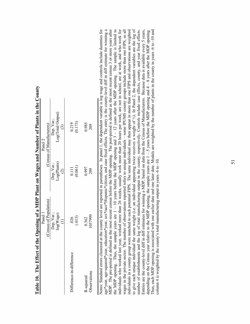
51
Tab
le 1
0. T
he E
ffec
t of t
he O
peni
ng o
f a M
DP
Plan
t on
Wag
es a
nd N
umbe
r of
Pla
nts i
n th
e C
ount
y
Pa
nel 1
(C
ensu
s of P
opul
atio
n)
Pa
nel 2
(C
ensu
s of M
anuf
actu
rers
)
Dep
. Var
.:
lo
g(W
age)
D
ep. V
ar.:
Log(
Plan
ts)
Dep
. Var
.:
Log(
Tota
l Out
put)
(1
)
(2
) (3
)
D
iffer
ence
-in-d
iffer
ence
.
026
0.11
1 0.
219
(.0
13)
(0.0
61)
(0.1
73)
R-s
quar
ed
0.36
2
0.
997
0.98
5
Obs
erva
tions
10
5799
9
20
9 20
9
N
otes
: Sta
ndar
d er
rors
clu
ster
ed a
t the
cou
nty
leve
l are
repo
rted
in p
aren
thes
es.
In p
anel
1, t
he d
epen
dent
var
iabl
e is
log
wag
e an
d co
ntro
ls in
clud
e du
mm
ies
for
age*
year
, age
-squ
ared
*yea
r, ed
ucat
ion*
year
, sex
*rac
e*H
ispa
nic*
citiz
en, a
nd c
ase
fixed
eff
ects
. The
ent
ry is
the
coun
ty-le
vel d
iff in
diff
est
imat
e fo
r win
ning
a
MD
P. T
he p
re-p
erio
d is
def
ined
as
the
mos
t rec
ent c
ensu
s be
fore
the
MD
P op
enin
g. T
he p
ost-p
erio
d is
def
ined
as
the
mos
t rec
ent c
ensu
s 3
or m
ore
year
s af
ter
the
MD
P op
enin
g.
Thus
, the
sam
ple
year
s ar
e 1
� 10
yea
rs b
efor
e th
e M
DP
open
ing
and
3 �
12 y
ears
afte
r th
e M
DP
open
ing.
Th
e sa
mpl
e is
lim
ited
to
indi
vidu
als
who
wor
ked
last
yea
r, w
orke
d m
ore
than
26
wee
ks, u
sual
ly w
ork
mor
e th
an 2
0 ho
urs
per
wee
k, a
re n
ot in
sch
ool,
are
at w
ork,
and
who
wor
k fo
r w
ages
in th
e pr
ivat
e se
ctor
. The
num
ber o
f obs
erva
tions
repo
rted
refe
rs to
uni
que
indi
vidu
als
� so
me
IPU
MS
coun
ty g
roup
s in
clud
e m
ore
than
one
FIP
S, s
o al
l in
divi
dual
s in
a c
ount
y gr
oup
wer
e m
atch
ed to
eac
h po
tent
ial F
IPS.
The
sam
e in
divi
dual
may
then
app
ear i
n m
ore
than
one
FIP
S an
d ob
serv
atio
ns a
re w
eigh
ted
to g
ive
each
uni
que
indi
vidu
al th
e sa
me
wei
ght (
i.e. a
n in
divi
dual
app
earin
g tw
ice
rece
ives
a w
eigh
t of
½).
In P
anel
2, t
he d
epen
dent
var
iabl
es a
re th
e lo
g of
nu
mbe
r of
est
ablis
hmen
ts a
nd th
e lo
g of
tota
l man
ufac
turin
g ou
tput
in th
e co
unty
, res
pect
ivel
y. C
ontro
ls in
clud
e ca
se e
ffec
ts, c
ount
y, a
nd y
ear
fixed
eff
ects
. En
tries
are
the
coun
ty-le
vel d
iff in
diff
est
imat
es fo
r win
ning
a M
DP,
bas
ed o
n da
ta fr
om th
e C
ensu
s of
Man
ufac
ture
rs.
Bec
ause
dat
a is
ava
ilabl
e ev
ery
5 ye
ars,
depe
ndin
g on
the
Cen
sus
year
rela
tive
to th
e M
DP
open
ing,
the
sam
ple
year
s ar
e 1
� 5
year
s be
fore
the
MD
P op
enin
g an
d 4
� 8
year
s af
ter t
he M
DP
open
ing.
Th
us, e
ach
MD
P op
enin
g is
ass
ocia
ted
with
one
ear
lier d
ate
and
one
late
r dat
e. M
odel
s ar
e w
eigh
ted
by th
e nu
mbe
r of p
lant
s in
the
coun
ty in
yea
rs -6
to -1
0 an
d co
lum
n 4
is w
eigh
ted
by th
e co
unty
�s to
tal m
anuf
actu
ring
outp
ut in
yea
rs -6
to -1
0.
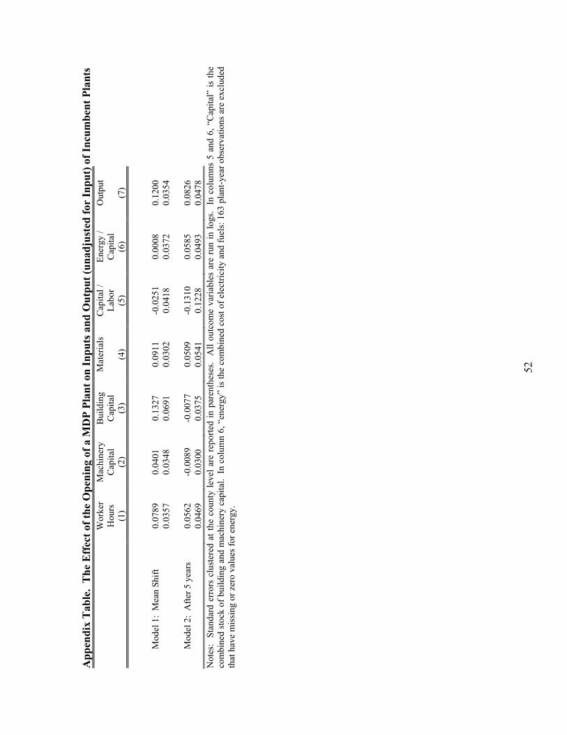
52
App
endi
x T
able
. T
he E
ffec
t of t
he O
peni
ng o
f a M
DP
Plan
t on
Inpu
ts a
nd O
utpu
t (un
adju
sted
for
Inpu
t) o
f Inc
umbe
nt P
lant
s
Wor
ker
Hou
rs
Mac
hine
ry
Cap
ital
Bui
ldin
g C
apita
l M
ater
ials
C
apita
l /
Labo
r En
ergy
/ C
apita
l O
utpu
t
(1
) (2
) (3
) (4
) (5
) (6
) (7
)
M
odel
1:
Mea
n Sh
ift
0.07
89
0.04
01
0.13
27
0.09
11
-0.0
251
0.00
08
0.12
00
0.
0357
0.
0348
0.
0691
0.
0302
0.
0418
0.
0372
0.
0354
M
odel
2:
Afte
r 5 y
ears
0.
0562
-0
.008
9 -0
.007
7 0.
0509
-0
.131
0 0.
0585
0.
0826
0.04
69
0.03
00
0.03
75
0.05
41
0.12
28
0.04
93
0.04
78
Not
es:
Stan
dard
err
ors
clus
tere
d at
the
coun
ty le
vel a
re r
epor
ted
in p
aren
thes
es.
All
outc
ome
varia
bles
are
run
in lo
gs.
In c
olum
ns 5
and
6, �
Cap
ital�
is th
e co
mbi
ned
stoc
k of
bui
ldin
g an
d m
achi
nery
cap
ital.
In c
olum
n 6,
�en
ergy
� is
the
com
bine
d co
st o
f ele
ctric
ity a
nd fu
els:
163
pla
nt-y
ear o
bser
vatio
ns a
re e
xclu
ded
that
hav
e m
issi
ng o
r zer
o va
lues
for e
nerg
y.