Identify the in uence of microstructure on mesoscale creep ...
70
ANL-20/49 Identify the influence of microstructure on mesoscale creep and fatigue damage Applied Materials Division
Transcript of Identify the in uence of microstructure on mesoscale creep ...
ANL-20/49
Identify the influence of microstructureon mesoscale creep and fatigue damage
Applied Materials Division

About Argonne National LaboratoryArgonne is a U.S. Department of Energy laboratory managed by UChicago Argonne, LLCunder contract DE-AC02-06CH11357. The Laboratory’s main facility is outside Chicago,at 9700 South Cass Avenue, Argonne, Illinois 60439. For information about Argonne andits pioneering science and technology programs, see www.anl.gov.
DOCUMENT AVAILABILITY
Online Access: U.S. Department of Energy (DOE) reports produced after 1991and a growing number of pre-1991 documents are available free at OSTI.GOV(http://www.osti.gov/), a service of the U.S. Dept. of Energy’s Office of Scientific andTechnical Information
Reports not in digital format may be purchased by the public from theNational Technical Information Service (NTIS):
U.S. Department of CommerceNational Technical Information Service5301 Shawnee RdAlexandria, VA 22312www.ntis.govPhone: (800) 553-NTIS (6847) or (703) 605-6000Fax: (703) 605-6900Email: [email protected]
Reports not in digital format are available to DOE and DOE contractors from theOffice of Scientific and Technical Information (OSTI)
U.S. Department of EnergyOffice of Scientific and Technical InformationP.O. Box 62Oak Ridge, TN 37831-0062www.osti.govPhone: (865) 576-8401Fax: (865) 576-5728Email: [email protected]
DisclaimerThis report was prepared as an account of work sponsored by an agency of the United States Government. Neither the United StatesGovernment nor any agency thereof, nor UChicago Argonne, LLC, nor any of their employees or officers, makes any warranty, express orimplied, or assumes any legal liability or responsibility for the accuracy, completeness, or usefulness of any information, apparatus,product, or process disclosed, or represents that its use would not infringe privately owned rights. Reference herein to any specificcommercial product, process, or service by trade name, trademark, manufacturer, or otherwise, does not necessarily constitute or implyits endorsement, recommendation, or favoring by the United States Government or any agency thereof. The views and opinions ofdocument authors expressed herein do not necessarily state or reflect those of the United States Government or any agency thereof,Argonne National Laboratory, or UChicago Argonne, LLC.
ANL-20/49
Identify the influence of microstructureon mesoscale creep and fatigue damage
Applied Materials DivisionArgonne National Laboratory
September 2020
Prepared by
A. Rovinelli, Argonne National LaboratoryM. C. Messner, Argonne National Laboratory

Identify the influence of microstructure on mesoscale creep and fatigue damageSeptember 2020
Abstract
This report describes the development of a microstructural model that can quantify theuncertainty in the observed rupture life of Grade 91 steel. The model is microstructural,meaning it relates microstructural characteristics of the material to the resulting materialresponse. As such, one of the uses of this model is to identify the key microstructural param-eters controlling the development of damage in Grade 91 operating at elevated temperatures.The report describes two veins of work: improvements to the crystal plasticity model requiredto run the uncertainty quantification analysis and the results of that UQ analysis. For creep,the model identifies the grain boundary diffusivity as the critical parameter controlling therupture life of the material. The report demonstrates that a reasonable microstructural dis-tribution of grain boundary diffusivity can account for the observed macroscale variation inrupture life at fixed temperature and load.
ANL-20/49 i


Identify the influence of microstructure on mesoscale creep and fatigue damageSeptember 2020
Table of Contents
Abstract i
Table of Contents iii
List of Figures v
List of Tables vii
1 Introduction 1
2 Large Deformation Hill-Mandel Cell Conditions in MOOSE 52.1 Objective . . . . . . . . . . . . . . . . . . . . . . . . . . . . . . . . . . . . . 52.2 Enforcing cell average and Hill-Mandel conditions . . . . . . . . . . . . . . . 7
2.2.1 Previous work . . . . . . . . . . . . . . . . . . . . . . . . . . . . . . . 72.2.2 New formulation . . . . . . . . . . . . . . . . . . . . . . . . . . . . . 82.2.3 Problems with the basic formulation . . . . . . . . . . . . . . . . . . 9
2.3 Total Lagrangian kernel . . . . . . . . . . . . . . . . . . . . . . . . . . . . . 112.3.1 Residual equation . . . . . . . . . . . . . . . . . . . . . . . . . . . . . 112.3.2 Jacobian terms . . . . . . . . . . . . . . . . . . . . . . . . . . . . . . 112.3.3 Verification . . . . . . . . . . . . . . . . . . . . . . . . . . . . . . . . 12
2.4 Verification . . . . . . . . . . . . . . . . . . . . . . . . . . . . . . . . . . . . 142.5 Identification of periodic boundaries . . . . . . . . . . . . . . . . . . . . . . . 15
3 Large deformation cohesive zone model in MOOSE 193.1 Implementation in MOOSE . . . . . . . . . . . . . . . . . . . . . . . . . . . 21
3.1.1 Cohesive model residual . . . . . . . . . . . . . . . . . . . . . . . . . 213.1.2 Cohesive model Jacobian . . . . . . . . . . . . . . . . . . . . . . . . . 22
3.2 Validation . . . . . . . . . . . . . . . . . . . . . . . . . . . . . . . . . . . . . 263.2.1 Objective traction rate validation . . . . . . . . . . . . . . . . . . . . 263.2.2 Cohesive zone model Jacobian validation . . . . . . . . . . . . . . . . 26
4 Constitutive models 334.1 The prior austenite grain model . . . . . . . . . . . . . . . . . . . . . . . . . 334.2 Grain boundary cavitation model . . . . . . . . . . . . . . . . . . . . . . . . 34
5 Identification of microstructural parameters influencing creep rupture life 395.1 Sensitivity analysis . . . . . . . . . . . . . . . . . . . . . . . . . . . . . . . . 395.2 Identifying parameters distributions . . . . . . . . . . . . . . . . . . . . . . . 45
6 Conclusions and future work 49
Acknowledgments 51
Bibliography 53
ANL-20/49 iii

Identify the influence of microstructure on mesoscale creep and fatigue damageSeptember 2020
List of Figures
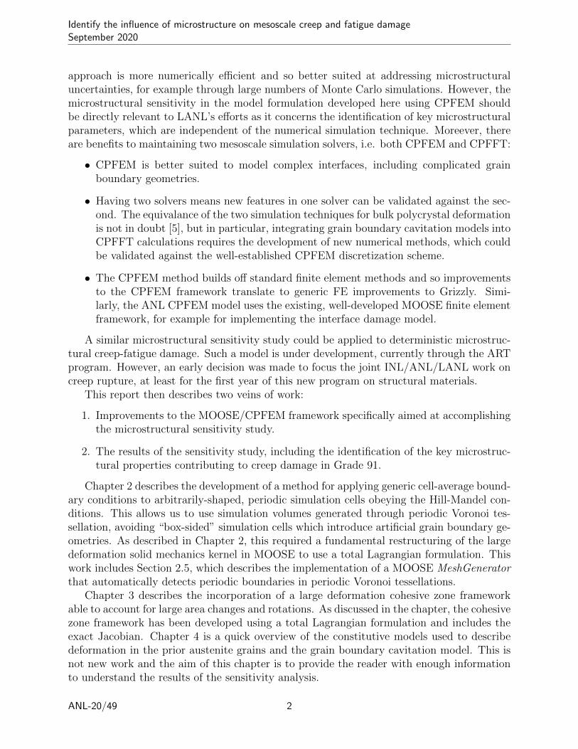
2.1 Illustration of the potential problems with box-sided representative cells. (a)Box-sided cell. (b) Equivalent true-periodic cell. (c) Periodic tiling of thebox-sided cell with the artificially implied grain boundaries highlighted. (d)Periodic tiling of the true-periodic cell. The highlighted periodic grain bound-aries are realistic. . . . . . . . . . . . . . . . . . . . . . . . . . . . . . . . . . 6
2.2 Comparison between the updated and total Lagrangian formulations for asimple forming problem. (a) Deformed shape for the updated Lagrangianformulation. (b) Deformed shape for the total Lagrangian formulation. (c)Total dissipated energy (work) plotted as a function of bend angle for the twoformulations. The two lines exactly overlap. . . . . . . . . . . . . . . . . . . 13
2.3 (a) Simple truncated octahedron cell for the verification calculation. (b)Demonstration that the cell remains periodic after significant deformation. . 13
2.4 Plots of the cell-average stress and deformation, demonstrating that the modelobeys the imposed constraints. . . . . . . . . . . . . . . . . . . . . . . . . . . 14
2.5 Render of a synthetic periodic microstructures with 100 grains, generated withNeper, colored by grain number. . . . . . . . . . . . . . . . . . . . . . . . . 15
2.6 Render of a synthetic periodic microstructures highlighting the identified pe-riodic surfaces. Different colors are associated to different periodic surfaces.. . . . . . . . . . . . . . . . . . . . . . . . . . . . . . . . . . . . . . . . . . . 17
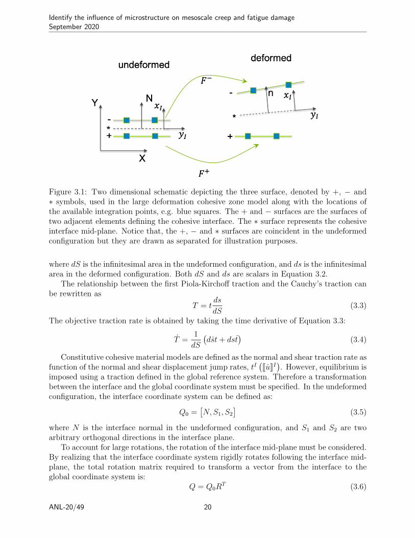
3.1 Two dimensional schematic depicting the three surface, denoted by +, − and∗ symbols, used in the large deformation cohesive zone model along with thelocations of the available integration points, e.g. blue squares. The + and− surfaces are the surfaces of two adjacent elements defining the cohesiveinterface. The ∗ surface represents the cohesive interface mid-plane. Noticethat, the +, − and ∗ surfaces are coincident in the undeformed configurationbut they are drawn as separated for illustration purposes. . . . . . . . . . . . 20
3.2 Rendering of the simulation without the CZM interface at different point intime. Axial stretching starts at time = 0 and ends a time = 1 . The 90 ◦ rigidbody rotation around the y axis starts at time = 1 and ends a time = 2 .The highlighted surface shows where the traction are computed. . . . . . . . 27
3.3 Comparison of the First Piola-Kirchoff traction for the two simulations withand without cohesive zone linear elastic model. Loading conditions are de-scribed in Figure 3.2. . . . . . . . . . . . . . . . . . . . . . . . . . . . . . . . 28
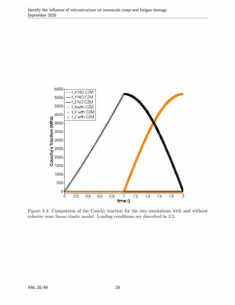
3.4 Comparison of the Cauchy traction for the two simulations with and withoutcohesive zone linear elastic model. Loading conditions are described in 3.2. . 29
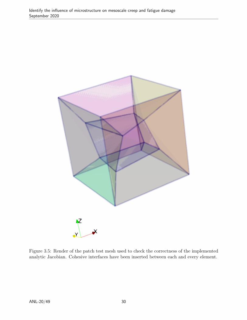
3.5 Render of the patch test mesh used to check the correctness of the implementedanalytic Jacobian. Cohesive interfaces have been inserted between each andevery element. . . . . . . . . . . . . . . . . . . . . . . . . . . . . . . . . . . . 30
4.1 Schematic representing the physical meaning of the grain boundary cavitationmodel state variables. The variable a represents the average cavity half radius,and the variable b represents the average cavity half spacing. . . . . . . . . . 35
ANL-20/49 v

Identify the influence of microstructure on mesoscale creep and fatigue damageSeptember 2020
5.1 Experimentally observed distribution of Grade 91 creep rupture life at 600 ◦Cfor a nominal stress of 100 MPa. The black line represents simulation results 40
5.2 Schematic representing box-periodic boundary conditions for uniaxial creeploading. The colored block represents the RVE and each color represents agrain. TZ is the nominal traction and corresponds to a constant applied force. 41
5.3 Rendering of simulation results for uniaxial creep and a nominal stress of100 MPa. . . . . . . . . . . . . . . . . . . . . . . . . . . . . . . . . . . . . . . 42
5.4 Sensitivity of different failure metrics with respect to the model parameterswhen performing a one-at-a-time sensitivity analysis. The failure metrics are:i) time to 1 % interface strain (TT1), ii) time to 2 % interface strain (TT2),and iii) time to 3 % interface strain (TT3). Sensitivity is plotted in log space. 44
5.5 Computed time to failure, using the time to 1 % interface strain metric, asfunction of the grain boundary diffusivity. . . . . . . . . . . . . . . . . . . . 45
5.6 The numerically computed grain boundary diffusivity distribution. Verticalline represent the calibrated DGB value. The blue line represents a smoothdistribution calculated using the kernel density estimation. . . . . . . . . . . 46
5.7 Normalized grain boundary energy. The dashed line shows the variability ofthe energy for random grain boundaries. Data from [31] . . . . . . . . . . . . 47
ANL-20/49 vi

Identify the influence of microstructure on mesoscale creep and fatigue damageSeptember 2020
List of Tables
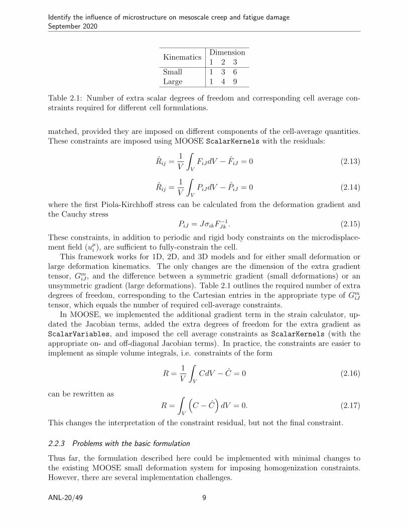
2.1 Number of extra scalar degrees of freedom and corresponding cell averageconstraints required for different cell formulations. . . . . . . . . . . . . . . . 9
3.1 Comparison of number of nonlinear iteration required to achieve convergencewhen using: i) the finite difference calculated Jacobian (column FDJ), and ii)the analytic Jacobian (column AJ). . . . . . . . . . . . . . . . . . . . . . . . 31
4.1 Grain bulk material parameters. . . . . . . . . . . . . . . . . . . . . . . . . . 344.2 Grain boundary cavitation material parameters. . . . . . . . . . . . . . . . . 37
ANL-20/49 vii

Identify the influence of microstructure on mesoscale creep and fatigue damageSeptember 2020
1 Introduction
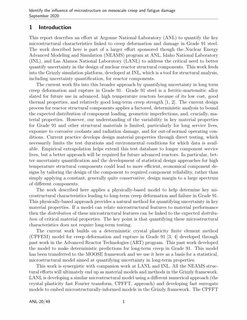
This report describes an effort at Argonne National Laboratory (ANL) to quantify the keymicrostructural characteristics linked to creep deformation and damage in Grade 91 steel.The work described here is part of a larger effort sponsored though the Nuclear EnergyAdvanced Modeling and Simulation (NEAMS) program at ANL, Idaho National Laboratory(INL), and Las Alamos National Laboratory (LANL) to address the critical need to betterquantify uncertainty in the design of nuclear reactor structural components. This work feedsinto the Grizzly simulation platform, developed at INL, which is a tool for structural analysis,including uncertainty quantification, for reactor components.
The current work fits into this broader approach by quantifying uncertainty in long termcreep deformation and rupture in Grade 91. Grade 91 steel is a ferritic-martensitic alloyslated for future use in advanced, high temperature reactors because of its low cost, goodthermal properties, and relatively good long-term creep strength [1, 2]. The current designprocess for reactor structural components applies a factored, deterministic analysis to boundthe expected distribution of component loading, geometric imperfections, and, crucially, ma-terial properties. However, our understanding of the variability in key material propertiesfor Grade 91 and other structural materials is limited, particularly for long service lives,exposure to corrosive coolants and radiation damage, and for out-of-normal operating con-ditions. Current practice develops design material properties through direct testing, whichnecessarily limits the test durations and environmental conditions for which data is avail-able. Empirical extrapolation helps extend this test database to longer component servicelives, but a better approach will be required for future advanced reactors. In particular, bet-ter uncertainty quantification and the development of statistical design approaches for hightemperature structural components could lead to more efficient, economical component de-signs by tailoring the design of the component to required component reliability, rather thansimply applying a constant, generally quite conservative, design margin to a large spectrumof different components.
The work described here applies a physically-based model to help determine key mi-crostructural characteristics leading to long-term creep deformation and failure in Grade 91.This physically-based approach provides a natural method for quantifying uncertainty in keymaterial properties. If a model can relate microstructural features to material performancethen the distribution of these microstructural features can be linked to the expected distribu-tion of critical material properties. The key point is that quantifying these microstructuralcharacteristics does not require long-term testing.
The current work builds on a deterministic crystal plasticity finite element method(CPFEM) model for creep deformation and rupture in Grade 91 [3, 4] developed throughpast work in the Advanced Reactor Technologies (ART) program. This past work developedthe model to make deterministic predictions for long-term creep in Grade 91. This modelhas been transferred to the MOOSE framework and we use it here as a basis for a statistical,microstructural model aimed at quantifying uncertainty in long-term properties.
This work is synergistic with companion work at LANL and INL. All the NEAMS struc-tural efforts will ultimately end up as material models and methods in the Grizzly framework.LANL is developing a similar microstructural model using a different numerical approach (thecrystal plasticity fast Fourier transform, CPFFT, approach) and developing fast surrogatemodels to embed microstructurally-informed models in the Grizzly framework. The CPFFT
ANL-20/49 1
Identify the influence of microstructure on mesoscale creep and fatigue damageSeptember 2020
approach is more numerically efficient and so better suited at addressing microstructuraluncertainties, for example through large numbers of Monte Carlo simulations. However, themicrostructural sensitivity in the model formulation developed here using CPFEM shouldbe directly relevant to LANL’s efforts as it concerns the identification of key microstructuralparameters, which are independent of the numerical simulation technique. Moreever, thereare benefits to maintaining two mesoscale simulation solvers, i.e. both CPFEM and CPFFT:
• CPFEM is better suited to model complex interfaces, including complicated grainboundary geometries.
• Having two solvers means new features in one solver can be validated against the sec-ond. The equivalance of the two simulation techniques for bulk polycrystal deformationis not in doubt [5], but in particular, integrating grain boundary cavitation models intoCPFFT calculations requires the development of new numerical methods, which couldbe validated against the well-established CPFEM discretization scheme.
• The CPFEM method builds off standard finite element methods and so improvementsto the CPFEM framework translate to generic FE improvements to Grizzly. Simi-larly, the ANL CPFEM model uses the existing, well-developed MOOSE finite elementframework, for example for implementing the interface damage model.
A similar microstructural sensitivity study could be applied to deterministic microstruc-tural creep-fatigue damage. Such a model is under development, currently through the ARTprogram. However, an early decision was made to focus the joint INL/ANL/LANL work oncreep rupture, at least for the first year of this new program on structural materials.
This report then describes two veins of work:
1. Improvements to the MOOSE/CPFEM framework specifically aimed at accomplishingthe microstructural sensitivity study.
2. The results of the sensitivity study, including the identification of the key microstruc-tural properties contributing to creep damage in Grade 91.
Chapter 2 describes the development of a method for applying generic cell-average bound-ary conditions to arbitrarily-shaped, periodic simulation cells obeying the Hill-Mandel con-ditions. This allows us to use simulation volumes generated through periodic Voronoi tes-sellation, avoiding “box-sided” simulation cells which introduce artificial grain boundary ge-ometries. As described in Chapter 2, this required a fundamental restructuring of the largedeformation solid mechanics kernel in MOOSE to use a total Lagrangian formulation. Thiswork includes Section 2.5, which describes the implementation of a MOOSE MeshGeneratorthat automatically detects periodic boundaries in periodic Voronoi tessellations.
Chapter 3 describes the incorporation of a large deformation cohesive zone frameworkable to account for large area changes and rotations. As discussed in the chapter, the cohesivezone framework has been developed using a total Lagrangian formulation and includes theexact Jacobian. Chapter 4 is a quick overview of the constitutive models used to describedeformation in the prior austenite grains and the grain boundary cavitation model. This isnot new work and the aim of this chapter is to provide the reader with enough informationto understand the results of the sensitivity analysis.
ANL-20/49 2

Identify the influence of microstructure on mesoscale creep and fatigue damageSeptember 2020
Chapter 5 describes the methodology used to model the experimental uncertainty in thecreep-rupture life of Grade 91 steel. Section 5.1 identifies the key microstructural parametersthrough sensitivity analysis and relates those parameters to the physics embedded in themicrostructural model. The sensitivity study shows that the controlling model parameteris the grain boundary diffusivity. Section 5.2 describes how the sensitivity analysis resultsare used to identify the model parameter distributions that explain the macroscale rupturedata. Results of this section show that accounting for the uncertainty of the grain boundarydiffusivity is sufficient to capture the experimental uncertainty of the creep-rupture life ofGrade 91.
Finally, Chapter 6 summarizes the work and describes the remaining work required toaccount for additional sources of uncertainty, such as the second phase particle distributionat the prior austenite grain boundaries.
ANL-20/49 3


Identify the influence of microstructure on mesoscale creep and fatigue damageSeptember 2020
2 Large Deformation Hill-Mandel Cell Conditions in MOOSE
2.1 Objective
Figure 2.1 shows two notionally-identical simulation cells, intended for use as periodic repre-sentative volumes in a microstructural simulation. Both were generated using the Neper [6]tool for producing representative microstructures using periodic Voronoi tessellation. Bothmicrostructures have identical grain orientations and grain shapes within the cell. Bothare periodic in the sense that both cells will tile space. The difference is Figure 2.1(a) is“box-sided” – the tessellation was truncated to make a cubic cell. Figure 2.1(b) is the fullyperiodic tessellation.
This chapter discusses changes to MOOSE required to run simulations based on cells likeFigure 2.1(b). Figure 2.1 (c) and (d) illustrates the reason why. Box-sided cells introduce aset of grain boundaries on the cell faces with an unphysical geometry — an entire plane ofaligned grain boundaries — whereas the true-periodic cells do not introduce similar sets ofplanar boundaries. These artificial boundaries are not important for simulations includingonly grain bulk deformation. However, they can be important for simulations with grainboundary physics, like the creep cavitation model. The entire set of boundaries could, forexample, directly align with the applied stress, creating a weak plane in the simulated volume.
Running simulations with these types of cells, in the context of proper homogenizationtheory, requires two conditions:
1. The cell obeys the classical Hill-Mandel condition.
2. A mechanism for enforcing arbitrary cell-averaged conditions on the simulation. Ideallythese conditions would include arbitrary combinations of stress and strain constraintsin different directions.
This chapter describes a mechanism for enforcing both conditions in MOOSE in the contextof large deformation kinematics.
The Hill-Mandel condition [7, 8] provides the necessary condition for the admissibility ofthe homogenized stress and deformation fields:
〈σ : D〉 = 〈σ〉 : 〈D〉 (2.1)
where σ is the Cauchy stress, D is the deformation rate, and
〈X〉 =1
V
∫V
XdV . (2.2)
Typically, models enforce the Hill-Mandel constraint using boundary conditions on the sim-ulation cell surface. There are many cell conditions that meet the Hill-Mandel condition,but the most common are:
1. Uniform traction BC: σ · n = t
2. Uniform displacement BC: u = u
3. Periodic displacements: u+ − u− = 0, where + and − indicate two pairs of periodicfaces.
ANL-20/49 5
Identify the influence of microstructure on mesoscale creep and fatigue damageSeptember 2020
Figure 2.1: Illustration of the potential problems with box-sided representative cells. (a)Box-sided cell. (b) Equivalent true-periodic cell. (c) Periodic tiling of the box-sided cellwith the artificially implied grain boundaries highlighted. (d) Periodic tiling of the true-periodic cell. The highlighted periodic grain boundaries are realistic.
ANL-20/49 6

Identify the influence of microstructure on mesoscale creep and fatigue damageSeptember 2020
Periodic boundary conditions are often the most efficient in determining effective propertiesfrom small representative volume elements. As such, this chapter seeks a solution thatimposes periodic conditions together with imposed cell-average constraints.
In addition to these boundary conditions some types of uniform cell conditions also satisfythe constraint:
1. Uniform stress: the Ruess bound
2. Uniform deformation: the Voigt bound.
Superpositions of these conditions will also satisfy the Hill-Mandel condition.For large deformations, cell-average constraints take the form:
σij =1
V
∫V
σijdV (2.3)
Fij =1
V
∫V
FijdV (2.4)
However, creep conditions impose a fixed dead load on the specimen, not a fixed Cauchystress. So instead, this chapter focuses on stress constraints of the type
Pij =1
V
∫V
PijdV (2.5)
where Pij is the first Piola-Kirchhoff stress, instead of the Cauchy stress in Eq. 2.3. Fixingthe first Piola-Kirchhoff stress imposes a constant dead load on the simulation cell.
Note that both deformation and stress constraints can be applied simultaneously providedthey are imposed in different directions (i.e. the indices ij are different). In addition, the cellrigid body translation and rotations must be removed, as described in further detail below.
2.2 Enforcing cell average and Hill-Mandel conditions
2.2.1 Previous work
A previous version of the ANL model, embedded in a different solver (WARP3D, http://www.warp3d.net/) implemented the cell average and Hill-Mandel constraints with a unifiedapproach, described in [9]. The idea is to enforce face-face constraints of the type:
u+ − u− =(F− I
)· (X+ −X−) (2.6)
where X+ and X− are the coordinates of the periodic faces in the undeformed configuration.The trick in this approach is to let the deformation conditions be extra, dummy degrees offreedom, often implemented as dummy nodes in the finite element mesh:
u?ij = Fij − δij. (2.7)
With this formulation, applying Dirichlet boundary conditions to the dummy degrees offreedom imposes cell-average deformation conditions, as Eq. 2.6 directly suggests, while
ANL-20/49 7
Identify the influence of microstructure on mesoscale creep and fatigue damageSeptember 2020
imposing Neumann boundary conditions applies components of the volume-integrated firstPiola-Kirchhoff stress, i.e.
∫VPijdV .
The WARP3D implementation imposed Eq. 2.6 using multipoint constraints. Note theconditions are true multipoint constraints as they will generally involve displacement compo-nents from the two faces and the dummy degrees of freedom. The current MOOSE constraintsystem is unsuited for implementing these types of conditions in 3D and so we examinedother approaches. These conditions can be rephrased as Lagrange multiplier constraints im-posed on nonlinear equations describing the unconstrained cell. In theory, there is no reasonwhy this implementation should not work in MOOSE, using scalar kernels to impose theLagrange multiplier equations. However, a trial ANL implementation was not numericallystable, and so we considered a third option.
2.2.2 New formulation
A superposition of conditions which individually meet the Hill-Mandel constraint also meetsthe constraint. One way to enforce a combination of cell-average conditions and the Hill-Mandel condition is to divide the displacement field into two components:
ui = uµi + uMi (2.8)
where the microdisplacement field (uµi ) obeys periodic boundary conditions and the macrodis-placement field (uMi ) is affine with some imposed deformation, i.e.
uMi = GiJXJ . (2.9)
The constant deformation GiJ represents 6 (3D, small deformation theory) or 9 (3D, largedeformation theory) extra degrees of freedom. These extra degrees of freedom correspondto the extra constraint equations required to set the cell average stress or deformation con-ditions.
MOOSE already implements a version of this scheme to impose homogenization condi-tions on cell simulations for small deformation kinematics. Unfortunately, extending thisimplementation to large deformation kinematics is not trivial.
In theory, the additions to the MOOSE material and tensor mechanics kernel system arestraightforward. Whenever the gradient of the displacements
ui,J (2.10)
appears replace it with the expression
ui,J = uµi,J +GmiJ (2.11)
whereGmiJ is a constant tensor field, represented with an appropriate number of ScalarVariables
in MOOSE. Note the deformation gradient simply becomes
FiJ = δiJ + ui,J = δiJ + uµi,J +GmiJ . (2.12)
The implementation supplements this addition to the model kinematics with the appropriatenumber of cell-average constraints. Deformation and stress constraints can be mixed and
ANL-20/49 8
Identify the influence of microstructure on mesoscale creep and fatigue damageSeptember 2020
KinematicsDimension1 2 3
Small 1 3 6Large 1 4 9
Table 2.1: Number of extra scalar degrees of freedom and corresponding cell average con-straints required for different cell formulations.
matched, provided they are imposed on different components of the cell-average quantities.These constraints are imposed using MOOSE ScalarKernels with the residuals:
Rij =1
V
∫V
FiJdV − FiJ = 0 (2.13)
Rij =1
V
∫V
PiJdV − PiJ = 0 (2.14)
where the first Piola-Kirchhoff stress can be calculated from the deformation gradient andthe Cauchy stress
PiJ = JσikF−1Jk . (2.15)
These constraints, in addition to periodic and rigid body constraints on the microdisplace-ment field (uµi ), are sufficient to fully-constrain the cell.
This framework works for 1D, 2D, and 3D models and for either small deformation orlarge deformation kinematics. The only changes are the dimension of the extra gradienttensor, Gm
iJ , and the difference between a symmetric gradient (small deformations) or anunsymmetric gradient (large deformations). Table 2.1 outlines the required number of extradegrees of freedom, corresponding to the Cartesian entries in the appropriate type of Gm
iJ
tensor, which equals the number of required cell-average constraints.In MOOSE, we implemented the additional gradient term in the strain calculator, up-
dated the Jacobian terms, added the extra degrees of freedom for the extra gradient asScalarVariables, and imposed the cell average constraints as ScalarKernels (with theappropriate on- and off-diagonal Jacobian terms). In practice, the constraints are easier toimplement as simple volume integrals, i.e. constraints of the form
R =1
V
∫V
CdV − C = 0 (2.16)
can be rewritten as
R =
∫V
(C − C
)dV = 0. (2.17)
This changes the interpretation of the constraint residual, but not the final constraint.
2.2.3 Problems with the basic formulation
Thus far, the formulation described here could be implemented with minimal changes tothe existing MOOSE small deformation system for imposing homogenization constraints.However, there are several implementation challenges.
ANL-20/49 9
Identify the influence of microstructure on mesoscale creep and fatigue damageSeptember 2020
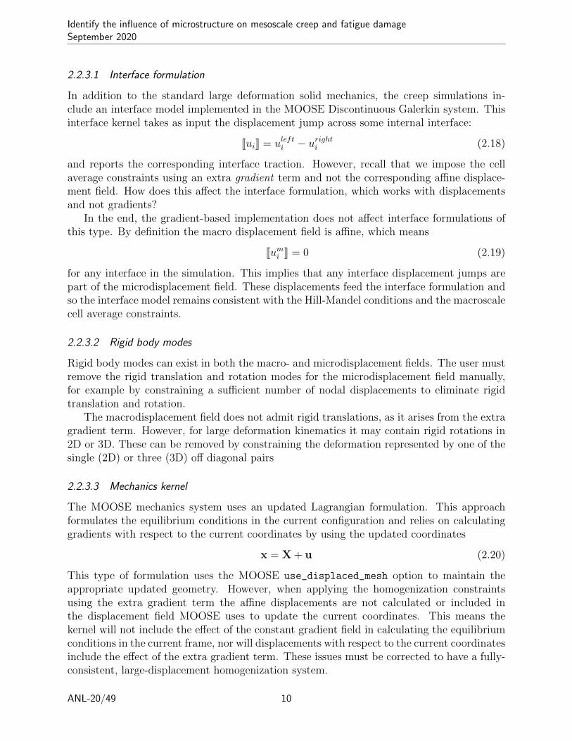
2.2.3.1 Interface formulation
In addition to the standard large deformation solid mechanics, the creep simulations in-clude an interface model implemented in the MOOSE Discontinuous Galerkin system. Thisinterface kernel takes as input the displacement jump across some internal interface:
JuiK = ulefti − urighti (2.18)
and reports the corresponding interface traction. However, recall that we impose the cellaverage constraints using an extra gradient term and not the corresponding affine displace-ment field. How does this affect the interface formulation, which works with displacementsand not gradients?
In the end, the gradient-based implementation does not affect interface formulations ofthis type. By definition the macro displacement field is affine, which means
Jumi K = 0 (2.19)
for any interface in the simulation. This implies that any interface displacement jumps arepart of the microdisplacement field. These displacements feed the interface formulation andso the interface model remains consistent with the Hill-Mandel conditions and the macroscalecell average constraints.
2.2.3.2 Rigid body modes
Rigid body modes can exist in both the macro- and microdisplacement fields. The user mustremove the rigid translation and rotation modes for the microdisplacement field manually,for example by constraining a sufficient number of nodal displacements to eliminate rigidtranslation and rotation.
The macrodisplacement field does not admit rigid translations, as it arises from the extragradient term. However, for large deformation kinematics it may contain rigid rotations in2D or 3D. These can be removed by constraining the deformation represented by one of thesingle (2D) or three (3D) off diagonal pairs
2.2.3.3 Mechanics kernel
The MOOSE mechanics system uses an updated Lagrangian formulation. This approachformulates the equilibrium conditions in the current configuration and relies on calculatinggradients with respect to the current coordinates by using the updated coordinates
x = X + u (2.20)
This type of formulation uses the MOOSE use_displaced_mesh option to maintain theappropriate updated geometry. However, when applying the homogenization constraintsusing the extra gradient term the affine displacements are not calculated or included inthe displacement field MOOSE uses to update the current coordinates. This means thekernel will not include the effect of the constant gradient field in calculating the equilibriumconditions in the current frame, nor will displacements with respect to the current coordinatesinclude the effect of the extra gradient term. These issues must be corrected to have a fully-consistent, large-displacement homogenization system.
ANL-20/49 10
Identify the influence of microstructure on mesoscale creep and fatigue damageSeptember 2020
2.3 Total Lagrangian kernel
We elected to rewrite the MOOSE large displacement solid mechanics kernel system to referonly to the reference configuration (i.e. a total Lagrangian formulation). This eliminates theneed for the use_displaced_mesh flag and means that the effects of the extra homogeniza-tion gradient term are included in the kinematic formulation.
2.3.1 Residual equation
The residual equation for the total Lagrangian formulation is
Rα =
∫V
Jσijφαi,KF
−1KjdV (2.21)
where J = detF and φ are the test functions. This formulates the equilibrium condi-tions in the undeformed configuration and only requires gradients with respect to the initialcoordinates. Therefore, the total Lagrangian kernel will integrate correctly with the homog-enization described above.
It is more common when working with a total Lagrangian formulation to note that
JσijF−1Kj = PiK (2.22)
and so
Rα =
∫V
PiKφαi,KdV = 0 (2.23)
and then make the constitutive model system responsible for returning the first Piola-Kirchhoff stress instead of the Cauchy stress. However, both the NEML and MOOSE consti-tutive model systems return the Cauchy stress and so our implementation keeps the longer,Cauchy stress form of Eq. 2.21. This means that the material systems for the original,updated formulation and the new, total formulation are the same. Two otherwise-identicalproblems using the two different kernel approaches should produce exactly the same results.
2.3.2 Jacobian terms
In the following Υβ are the discrete nodal displacements and ψ are the trial functions.The Jacobian has three terms:
∂Rα
∂Υβ=
∫V
(∂J
∂Υβσijφ
αi,KF
−1Kj + J
∂σij∂Υβ
φαi,KF−1Kj + Jσijφ
αi,K
∂F−1Kj
∂Υβ
)dV (2.24)
which we label for convenience:
Jαβ =
∫V
Aαβ +Bαβ + CαβdV (2.25)
Working term-by-term:
Aαβ = JF−1Lk ψ
βk,Lσijφ
αi,KF
−1Kj (2.26)
ANL-20/49 11
Identify the influence of microstructure on mesoscale creep and fatigue damageSeptember 2020
Bαβ = JCijmnF(n)mAF
−1As F
−1Tnψ
αs,Tφ
αi,KF
−1Kj (2.27)
which we could write
Bαβ = JCijmnf−1msF
−1Tnψ
αs,Tφ
αi,KF
−1Kj (2.28)
and finally
Cαβ = Jσijφαi,K
∂F−1Kj
∂FmN
∂FmN∂Υβ
= Jσijφαi,K
∂F−1Kj
∂FmNψβm,N (2.29)
Cαβ = −Jσijφαi,KF−1KmF
−1Njψ
βm,N (2.30)
We can combine the first and last terms and make simplifications:
Aαβ + Cαβ = JF−1Lk ψ
βk,Lσijφ
αi,KF
−1Kj − Jσijφαi,KF−1
KmF−1Njψ
βm,N (2.31)
Aαβ + Cαβ = Jφαi,KF−1Kjσijψ
βk,NF
−1Nk − Jφαi,KF−1
Kmσijψβm,NF
−1Nj (2.32)
Aαβ + Cαβ = Jσij
(ψβi,MF
−1Mjφ
αk,NF
−1Nk − ψβi,MF−1
Mkφαk,NF
−1Nj
)(2.33)
Aαβ + Cαβ = Jψβi,Mσijφαk,N
(F−1MjF
−1Nk − F−1
MkF−1Nj
)(2.34)
If we define:
Φαi,j = φαi,kF
−1k,j (2.35)
Ψβi,j = ψβi,kF
−1k,j (2.36)
then we have:
Bαβ = JCijmnf−1mkΨ
βk,nΦα
i,j (2.37)
Aαβ + Cαβ = Jσij
(Ψβi,jΦ
αk,k −Ψβ
i,kφαk,j
)(2.38)
2.3.3 Verification
As noted above, the updated and total Lagrangian kernels should produce identical resultsfor identical problems. Defining a verification case is straightforward as the two models canuse the same materials, boundary conditions, etc.
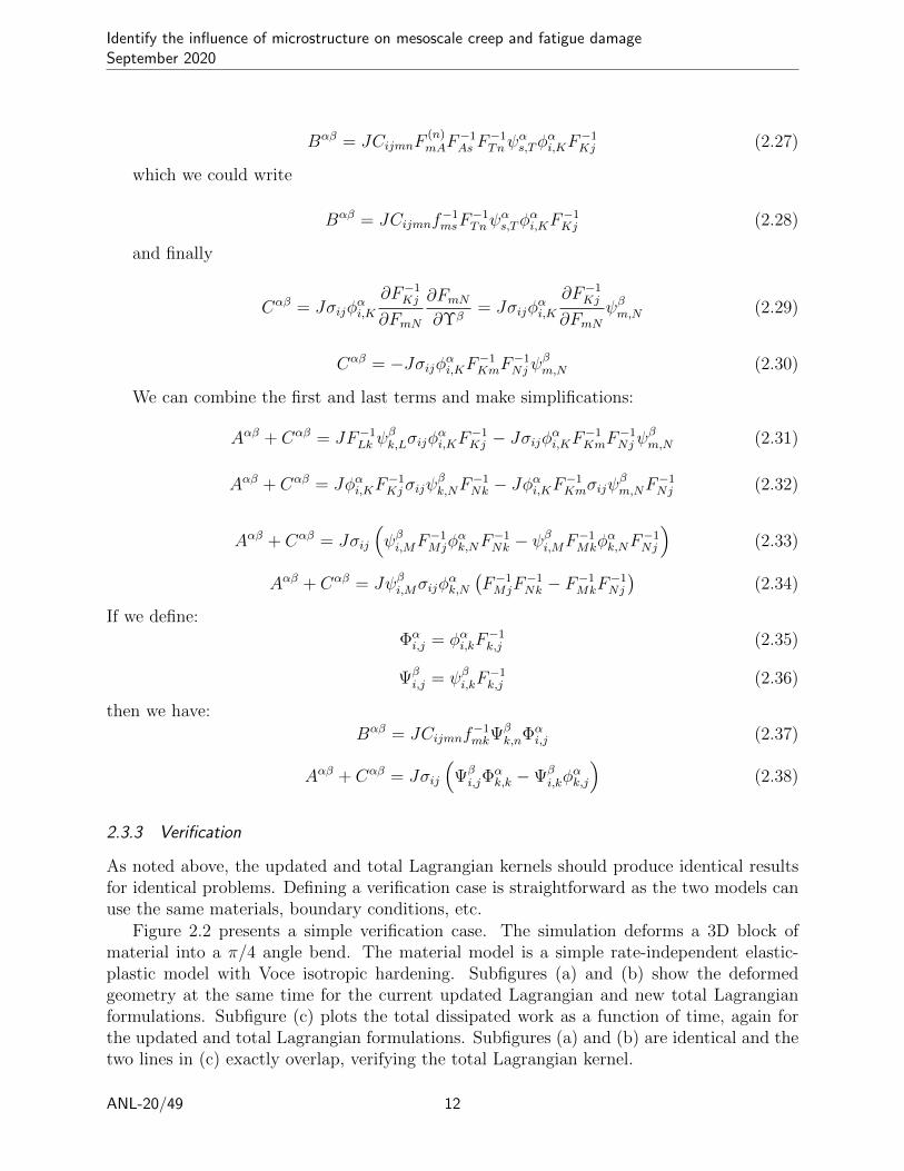
Figure 2.2 presents a simple verification case. The simulation deforms a 3D block ofmaterial into a π/4 angle bend. The material model is a simple rate-independent elastic-plastic model with Voce isotropic hardening. Subfigures (a) and (b) show the deformedgeometry at the same time for the current updated Lagrangian and new total Lagrangianformulations. Subfigure (c) plots the total dissipated work as a function of time, again forthe updated and total Lagrangian formulations. Subfigures (a) and (b) are identical and thetwo lines in (c) exactly overlap, verifying the total Lagrangian kernel.
ANL-20/49 12
Identify the influence of microstructure on mesoscale creep and fatigue damageSeptember 2020
(a) (b) (c)
Figure 2.2: Comparison between the updated and total Lagrangian formulations for a simpleforming problem. (a) Deformed shape for the updated Lagrangian formulation. (b) Deformedshape for the total Lagrangian formulation. (c) Total dissipated energy (work) plotted as afunction of bend angle for the two formulations. The two lines exactly overlap.
(a) (b)
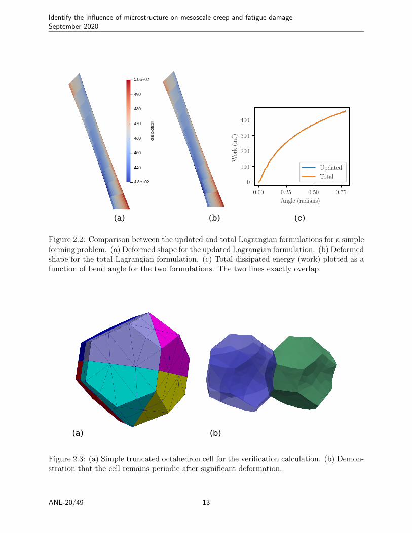
Figure 2.3: (a) Simple truncated octahedron cell for the verification calculation. (b) Demon-stration that the cell remains periodic after significant deformation.
ANL-20/49 13

Identify the influence of microstructure on mesoscale creep and fatigue damageSeptember 2020
0 2 4 6 8
Time
0
100
200S
tres
s
(a) First Piola-Kirchhoff stress.
0.0 2.5 5.0 7.5
Time
−0.2
0.0
0.2
0.4
Def
orm
atio
n
(b) Deformation
Figure 2.4: Plots of the cell-average stress and deformation, demonstrating that the modelobeys the imposed constraints.
2.4 Verification
Figure 2.3(a) shows a simple periodic cell consisting of 8 randomly oriented grains. The cellgeometry is simple, but deliberately setup to not have simple Cartesian periodicity. The3D model applies the homogenization system for large deformations with mixed constraints:three zero deformation constraints to remove rigid rotations, three average stress constraints,and three average deformation constraints. Figure 2.3(b) shows the deformed unit cell anddemonstrates that after deformation the cell remains periodic. Note that only the microdis-placements appear in the deformed volume rendering, as the macrodisplacements are neverexplicitly calculated. However, the macrodisplacement field is clearly periodic as it is affinewith the imposed gradient.
Finally, Figures 2.4(a) and (b) demonstrate that the average stress and deformation con-ditions match the applied values. Subfigure (a) plots the cell-average 1st Piola-Kirchhoffstress; subfigure (b) plots the average deformation (F − I). The constrained values appearas black lines in the diagrams. These were ramped linearly. The figures plot the uncon-strained values in blue. The cell averages match the constrained values, thus verifying thehomogenization system.
ANL-20/49 14

Identify the influence of microstructure on mesoscale creep and fatigue damageSeptember 2020
Figure 2.5: Render of a synthetic periodic microstructures with 100 grains, generated withNeper, colored by grain number.
2.5 Identification of periodic boundaries
MOOSE enforces periodic boundary conditions by imposing periodicity of a variable valueon periodic domain boundaries. For a rectangular cuboid cell MOOSE can identify the sixperiodic cell boundaries, and automatically choose the correct periodic pairs. However, formore complex periodic cell types the automatic periodic boundary detection feature can notbe used. Neper [6] generates complex periodic cell shapes like the one depicted in Figure2.5.
Furthermore, the periodic unit cells generated by Neper possess multiple periodic, non-flat, surfaces which can be characterized by the following families of translation directions:
• 〈001〉,
• 〈011〉,
• 〈111〉.The set of of all translation vector is obtained by applying the 24 cubic symmetries to allthe translation vector families and retaining the linearly independent set. This operation
ANL-20/49 15
Identify the influence of microstructure on mesoscale creep and fatigue damageSeptember 2020
generates a set of 13 independent translation vector. Each translation vector is associated toa pair of periodic, non-flat surfaces. In finite elements, a surface is represented by a collectionof element sides. Each element side is characterized by a set of nodes. Therefore, given aspecific translation direction, d two sides, s1 and s2, are periodic if the nodes describing themare translated by a distance d.
Given the above, a pseudo algorithm to identify periodic boundaries is the following:
1. find all the nodes on the surface of the periodic cell
2. for each node i loop over all the nodes, j, and check if they are periodic for any of thethirteen translation vector dk. If the node pair is periodic for direction dk, add node ito the list of nodes associated to the primary side of dk, and add node j to the list ofnodes associated the secondary side of dk. This process will generate a set of twentysix node sets.
3. for each node set, identify all the element-sides belonging to it and add them theassociated side-set.
Neper can generate periodic meshes that can be directly used as an input for MOOSE.Therefore to automate the process of creating periodic boundaries we develop a mesh gen-erator in MOOSE that identifies periodic boundaries, and automatically set all the requiredperiodic boundary conditions. Figure 2.6 is an example showing the identified periodic,non-flat boundaries.
We plan to merge this tool into MOOSE proper.
ANL-20/49 16

Identify the influence of microstructure on mesoscale creep and fatigue damageSeptember 2020
Figure 2.6: Render of a synthetic periodic microstructures highlighting the identified periodicsurfaces. Different colors are associated to different periodic surfaces.
ANL-20/49 17

Identify the influence of microstructure on mesoscale creep and fatigue damageSeptember 2020
3 Large deformation cohesive zone model in MOOSE
Libmesh [10], which is the finite element library on which MOOSE is built on [11] , does notsupport conventional interface elements. Therefore Messner et al. [12] utilized an elementlessdiscontinuous Galerkin approach for cohesive zone modeling in MOOSE. Rovinelli et al.[13] successfully used this method to perform physics-based crystal plasticity simulation,including grain boundary cavitation, to investigate the ability of different effective stressmeasures to predict the creep life of Grade 91 steel. However, the cohesive zone modelcurrently available in MOOSE does not account for large interface area changes and rotations.Creep rupture in ductile materials, such as Grade 91, occurs with area reduction factorsgrater than 80% [14], thus justifying the need for large deformation cohesive zone model inMOOSE.
To implement any large deformation constitutive model the deformation gradient F mustbe known. In general F can be computed at any integration point by using nodal displace-ments and shape functions. Standard cohesive zone modeling is not an exception as it relieson the knowing F on the cohesive interface. The cohesive interface is generally modeledwith cohesive elements [15]. Cohesive elements are a special type of zero-thickness elementsproviding integration points on their mid-plane. Most large deformation implementationsuse the mid-plane to define the cohesive separation law, which carries over to discontinuousGalerkin approaches [16]. These implementations also enforce traction equilibrium on themidplane.
However, the MOOSE DG formulation integrates over the element sides, which is achallenge for large deformations. The lack of integration points on the mid-plane forced usto use an assumption to recover the deformation gradient on the interface mid-plane. As afirst order approximation we assume the deformation gradient on the mid-plane, F ∗, to bethe average of the deformation gradient on the + and − surfaces:
F ∗ =F+ + F−
2. (3.1)
Figure 3.1 is a schematic representing the cohesive interface, ∗, and the surfaces of thetwo elements generating the cohesive interface together with the available quadrature points.
For large deformation problems, MOOSE allows equilibrium to be imposed on both thedeformed or the undeformed mesh. When solving a solid mechanics problem one has tosatisfy both the linear and angular momentum equilibrium. For equilibrium applied onthe undeformed configuration angular momentum is automatically satisfied because of thezero thickness interface assumption. If the formulation imposes equilibrium in the deformedconfiguration angular momentum conservation must be enforced with constraints on the co-hesive constitutive model. Note the analogy here with conventional solid mechanics: totalLagrangian formulations impose equilibrium in the undeformed configuration working withthe 1st Piola-Kirchhoff stress, which is a general rank 2 tensor. Updated Lagrangian formu-lations enforce equilibrium in the deformed configuration but the constitutive model mustmaintain a symmetric Cauchy stress to conserve angular momentum. We elected to use atotal Lagrangian formulation. The total Lagrangian formulation requires a map between thefirst Piola-Kirchoff traction, T , the Cauchy’s traction t and the infinitesimal force df . Thefollowing relationship defines the equivalence between, df , T and t:
df = TdS = tds (3.2)
ANL-20/49 19
Identify the influence of microstructure on mesoscale creep and fatigue damageSeptember 2020
Figure 3.1: Two dimensional schematic depicting the three surface, denoted by +, − and∗ symbols, used in the large deformation cohesive zone model along with the locations ofthe available integration points, e.g. blue squares. The + and − surfaces are the surfaces oftwo adjacent elements defining the cohesive interface. The ∗ surface represents the cohesiveinterface mid-plane. Notice that, the +, − and ∗ surfaces are coincident in the undeformedconfiguration but they are drawn as separated for illustration purposes.
where dS is the infinitesimal area in the undeformed configuration, and ds is the infinitesimalarea in the deformed configuration. Both dS and ds are scalars in Equation 3.2.
The relationship between the first Piola-Kirchoff traction and the Cauchy’s traction canbe rewritten as
T = tds
dS(3.3)
The objective traction rate is obtained by taking the time derivative of Equation 3.3:
T =1
dS
(dst+ dst
)(3.4)
Constitutive cohesive material models are defined as the normal and shear traction rate asfunction of the normal and shear displacement jump rates, tI
(JuKI
). However, equilibrium is
imposed using a traction defined in the global reference system. Therefore a transformationbetween the interface and the global coordinate system must be specified. In the undeformedconfiguration, the interface coordinate system can be defined as:
Q0 =[N,S1, S2
](3.5)
where N is the interface normal in the undeformed configuration, and S1 and S2 are twoarbitrary orthogonal directions in the interface plane.
To account for large rotations, the rotation of the interface mid-plane must be considered.By realizing that the interface coordinate system rigidly rotates following the interface mid-plane, the total rotation matrix required to transform a vector from the interface to theglobal coordinate system is:
Q = Q0RT (3.6)
ANL-20/49 20
Identify the influence of microstructure on mesoscale creep and fatigue damageSeptember 2020
where R is the rotation matrix accounting for the interface mid-plane rotation. The rotationmatrix Q can be used to rotate the displacement jump and the traction from the deformedinterface coordinate system to the global coordinate system as:
JuK = QT JuKI . (3.7)
t = QT tI . (3.8)
By differentiating Eq. 3.7 and 3.8 with respect to time one obtains:
JuK = QT JuKI +QT JuKI . (3.9)
t = QT tI +QT tI . (3.10)
Finally, substituting 3.8 and 3.10 in Eq. 3.4 one obtains:
T =ds
dS
((ds
dsQT + QT
)tI +QT tI
). (3.11)
Notice that Eq. 3.11 reduces to T = QT tI = t when large rotation and area changes areneglected (e.g., when ds = QT = 0 and ds
dS= 1), which is a consistency check. Equation
3.11 embeds all the kinematics, thus decoupling the kinematics from the traction-separationconstitutive equation. The traction separation constitutive equation is assumed to be definedin the interface mid-plane in the deformed configuration.
Decoupling the kinematics and constitutive equations greatly eases the implementationof custom traction separation laws because the only terms that need to be defined are:
• the material constitutive rate equations in the interface coordinate system and tI(JuKI
),
• the total derivatives of interface traction rates with respect to the interface displace-
ment jump,dtIidJuKIj
.
Equation 3.11 was implemented in the MOOSE cohesive zone model material system usingthe following incremental formulation:
∆T =ds
dS
((∆ds
dsQT + ∆QT
)tI +QT∆tI
). (3.12)
3.1 Implementation in MOOSE
3.1.1 Cohesive model residual
The residual equation for the total Lagrangian cohesive zone formulation for the displacementcomponent i can be written as:
Rα,+i = −
∫S
Ti (JuK)i φα,+i dS (3.13)
Rα,−i =
∫S
Ti (JuK)i φα,−i dS (3.14)
ANL-20/49 21
Identify the influence of microstructure on mesoscale creep and fatigue damageSeptember 2020
(3.15)
where α is the test function index and φ+ and φ− are the test function associated to the +and − surfaces, respectively. Notice that in the above equation i is not a summation index,but represents the coordinate i.
3.1.2 Cohesive model Jacobian
The Jacobian is the derivative of the residual with respect to the discrete displacementsΥβ. The traction on each side of the interface is a function of the displacement jump, JuK,therefore the residual on both element faces is function of the displacement on both sides ofinterface. This then requires the derivatives
dRα,+i
dΥβ,+j
= −∫S
dTi (JuK)φα,+i
dΥβ,+j
dS = −∫S
d∆Ti (JuK)dΥβ,+
j
φα,+i dS (3.16)
dRα,+i
dΥβ,−j
= −∫S
dTi (JuK)φα,+i
dΥβ,−j
dS = −∫S
d∆Ti (JuK)dΥβ,−
j
φα,+i dS (3.17)
dRα,−i
dΥβ,+j
=
∫S
dTi (JuK)φα,−idΥβ,+
j
dS =
∫S
d∆Ti (JuK)dΥβ,+
j
φα,+i dS (3.18)
dRα,−i
dΥβ,−j
=
∫S
dTi (JuK)φα,−idΥβ,−
j
dS =
∫S
d∆Ti (JuK)dΥβ,−
j
φα,+i dS (3.19)
In writing Eqs. 3.16 - 3.19 we have implicitly noticed that: i) dS is constant, ii) the testfunctions φα are independent from the discrete displacements, iii) Ti = Told,i + ∆Ti, and iv)Told,i is independent from the discrete displacements.
We start by recalling the finite element discretization for a variable:
u ≈ uh =∑β
Υβψβ (3.20)
where ψ indicates the trial function. By utilizing the displacement jump definition and thefinite element discretization, the displacement jump for the coordinate i can be expressedas:
JuKi = u−i − u+i ≈
∑β,−
Υβ,−i ψβ,−i −
∑β,+
Υβ,+i ψβ,+i (3.21)
The derivative of the displacement jump with respect to the discrete displacements can beapproximated as:
dJuKidΥβ,−
j
≈ ψβ,−i if i = j, else 0 (3.22)
dJuKidΥβ,+
j
≈ −ψβ,+i if i = j, else 0 (3.23)
(3.24)
ANL-20/49 22

Identify the influence of microstructure on mesoscale creep and fatigue damageSeptember 2020
where δij is the Kronecker delta. By noticing that the deformation gradients can be approx-imated as:
F+ij ≈ δij +
∑β
Υβ,+i ∇ψβ,+ij (3.25)
F−ij ≈ δij +∑β
Υβ,−i ∇ψβ,−ij (3.26)
where δij is the Kronecker delta. By using equation 3.1 the derivatives of F ∗ with respectto the discrete displacements becomes:
dF ∗ij
dΥβ,−k
≈ 1
2∇ψβ,−ij if k = i, else 0 (3.27)
dF ∗ij
dΥβ,+k
≈ 1
2∇ψβ,+ij if k = i, else 0 (3.28)
To simplify the Jacobian development, we define the following quantities:
A =ds
dS(3.29)
B =
(∆ds
dsQT + ∆QT
)(3.30)
C = QT (3.31)
and use them to rewrite Eq. 3.12 as:
∆T = A(BtI + C∆tI
)(3.32)
(3.33)
From Eqs. 3.16 - 3.19 is apparent that computing the Jacobian implies computing thefollowing derivatives:
d∆Ti (JuK)dΥβ,+
j
=d
dΥβ,+j
(A(Bikt
Ik + Cik∆t
Ik
))(3.34)
d∆Ti (JuK)dΥβ,−
j
=d
dΥβ,−j
(A(Bikt
Ik + Cik∆t
Ik
))(3.35)
By using the chain rule and doing some manipulation we obtain the following equations:
d∆Ti (JuK)∂Υβ,+
j
=∂A
dΥβ,+j
(Bikt
Ik + Cik∆t
Ik
)+ A
(∂Bik
∂Υβ,+j
tIk +∂Cik
∂Υβ,+j
∆tIk + (Bik + Cik)∂∆tIk∂Υβ,+
j
)(3.36)
d∆Ti (JuK)∂Υβ,−
j
=∂A
dΥβ,−j
(Bikt
Ik + Cik∆t
Ik
)+ A
(∂Bik
∂Υβ,−j
tIk +∂Cik
∂Υβ,−j
∆tIk + (Bik + Cik)∂∆tIk∂Υβ,−
j
)(3.37)
ANL-20/49 23
Identify the influence of microstructure on mesoscale creep and fatigue damageSeptember 2020
The remaining partial derivatives of A, B, and ∆tI can be computed by exploiting thechain rule again:
∂A
∂Υβ,+j
=∂A
∂F ∗rs
∂F ∗rs
∂Υβ,+j
∂A
∂Υβ,−j
=∂A
∂F ∗rs
∂F ∗rs
∂Υβ,−j
(3.38)
∂Bik
∂Υβ,+j
=∂Bik
∂F ∗rs
∂F ∗rs
∂Υβ,+j
∂Bik
∂Υβ,−j
=∂Bik
∂F ∗rs
∂F ∗rs
∂Υβ,−j
(3.39)
∂Cik
∂Υβ,+j
=∂Cik∂F ∗rs
∂F ∗rs
∂Υβ,+j
∂Cik
∂Υβ,−j
=∂Cik∂F ∗rs
∂F ∗rs
∂Υβ,−j
(3.40)
∂∆tIk∂Υβ,+
j
=∂∆tIk∂J∆uKIr
∂J∆uKIr∂JuKs
∂JuKs∂Υβ,+
j
∂∆tIk∂Υβ,−
j
=∂∆tIk∂J∆uKIr
∂J∆uKIr∂JuKs
∂JuKs∂Υβ,−
j
(3.41)
The partial derivatives of F ∗ and JuK with respect to the discrete displacements havealready been defined in Eqs. 3.22, 3.23, 3.27 and 3.28. The partial derivative of tI withrespect to JuKI is a material dependent derivative and will not be discussed here. By usingNanson’s Formula and adopting other kinematics identities we can recast A,B and C asfollows:
A =ds
dS= det (F )||F−TN || (3.42)
B =
(∆ds
dsQT + ∆QT
)=(
trace (L)− n · (Ln))RQT
0 + ∆RQT0 (3.43)
C = QT = RQT0 (3.44)
where we dropped the superscript ∗ of F to simplify the notation.We start by computing ∂C
∂Fas:
∂Cij∂Frs
=∂Rik
∂FrsQT
0,kj (3.45)
where the partial derivative of the rotation matrix can be computed using the formulaproposed by Chen and Wheeler [17]:
∂Rkl
∂Fmn=
Rkp
det(U) (UpqRmqUnl − UpnRmqUql
)(3.46)
where U = trace (U) I − U . The incremental model also requires to compute ∂∆Rkl
∂Fmn. In the
implementation we used a linear rotation approximation therefore ∆R = R−Rold. Noticingthat
∂Rold,kl
∂Fmn= 0 we obtain
∂∆Rij
∂Frs=∂Rij
∂Frs(3.47)
The next term we analyze is ∂A∂F
:
∂A
∂Fpq=∂ det (F )
∂Fpq||F−TN ||+ det (F )
∂||F−TN ||Fpq
(3.48)
ANL-20/49 24

Identify the influence of microstructure on mesoscale creep and fatigue damageSeptember 2020
The derivative of the determinant is
∂ det (F )
∂Fij= det (F )F−Tij (3.49)
The derivative of the norm can be computed by realizing that the derivative of the norm ofa vector with respect to its component is:
∂||V ||∂Vi
=Vi||V || (3.50)
and that the derivative of the inverse of a tensor with respect to its components is:
∂T−ij∂Tpq
= T−ipT−qj (3.51)
By using Eqs. 3.49, 3.50 and 3.51 and substituting in Eq. 3.48 we obtain:
∂A
∂Fpq= det (F )F−Tpq ||F−TN ||+ det (F )
F−Tik Nk
||F−TN ||F−jpF
−qiNj (3.52)
The other term for which we need to compute the partial derivatives is ∂B∂F
. By expandingthe partial derivatives and using the definition and derivatives of C (Eqs. 3.44 and 3.45) weobtain:
∂Bij
∂Fpq=
(∂ trace (L)
∂Fpq− ∂ (nrLrsns)
∂Fpq
)Cij +
(trace (L)− nrLrsns
)∂Cij∂Fpq
+∂Cij∂Fpq
(3.53)
In the incremental formulation L = I − FoldF− hence by using Eq. 3.51 we obtain.
∂Lij∂Fpq
= −Fold,ikF−kpF−qj . (3.54)
By noting the derivative of the trace of tensor with respect to its components is δij and usingEq. 3.54 the identity matrix, we can compute the derivate of velocity gradient with respectto the deformation gradient as:
∂ trace (L)
∂Fpq=∂ trace (L)
∂Lij
∂Lij∂Fpq
= −δijFold,ikF−kpF−qj (3.55)
Now we are left with computing the derivative of the second term inside the parentheses inEq. 3.53. By recalling that ni = RijNj and substituting we obtain:
∂ (nrLrsns)
∂Fpq=∂Rri
∂FpqNiLrsRsjNj +Rri
∂Lrs∂Fpq
RsjNj +RriNiLrsRsj∂Rsj
∂FpqNj (3.56)
where the partial derivatives on the right hand side can be computed using Eqs. 3.46 and3.54.
To complete the Jacobian definition, we need to compute the derivative of ∂J∆uKI
∂JuK presentin Equation 3.41. By using Eq. 3.7 we can write:
∂J∆uKIi∂JuKj
=∂ (∆QikJuKk +QikJ∆uKk)
∂JuKj= ∆Qikδkj +Qikδkj = ∆Qij +Qij (3.57)
where ∆Q = Q0∆RT . The complete Jacobian can now be computed by assembling all thederivates that has been identified in this section.
ANL-20/49 25

Identify the influence of microstructure on mesoscale creep and fatigue damageSeptember 2020
3.2 Validation
Validation of the objective traction rate was performed by using a simple linear elastictraction separation law:
∆Ti = KijJ∆uKIj (3.58)
where K is the interface stiffness matrix and is defined as:
K =
KN , 0, 00, KS, 00, 0, KS
(3.59)
with KN = 1 · 107 MPa/mm and KS = 1 · 107 MPa/mm. The solid elements have been modeledusing isotropic elasticity with a Young’s modulus of E = 1 · 104 MPa and a Poisson’s ratio ofν = 0.3. The values of the interface stiffness and bulk material properties have been selectedto allow deformations mainly in the bulk material.
3.2.1 Objective traction rate validation
To validate the objective traction rate formulation we compare two cases: i) one with acohesive interface, and ii) one without. If the traction objective rate is correct introducinga very stiff interface should not change the simulation results. Furthermore to check bothlarge rotations and large area changes, the simulation includes an initial axial strain up toan axial strain of 1 in the loading direction (z) and then a rigid rotation of 90 ◦ around the yaxis (see Figure 3.2). We compare both the first Piola-Kirchoff traction, T and the Cauchy’straction t. Figures 3.3 and 3.4 compares the first Piola-Kirchoof traction and Cauchy’straction for the two cases described above. The results of the two simulations are identicalthus confirming the correct implementation of the model and the validity of Eq. 3.1.
3.2.2 Cohesive zone model Jacobian validation
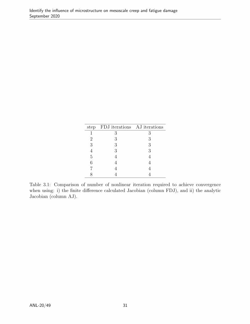
To evaluate the accuracy of the analytical Jacobian we utilized a classic patch test. We usedthe same material and interface model described in the previous section with similar loadingconditions (stretch and subsequent rotation). The patch test mesh is depicted in Figure 3.5To ensure the correctness of the implemented analytic Jacobian we compared the convergerate for two simulations using: i) the implemented analytic Jacobian, and ii) the Jacobiancomputed using finite differences. If for a patch test the same convergence rate are observedfor both cases then the analytic Jacobian is correct. Comparison of the number of nonlineariterations required to achieve convergence using both kinds of Jacobians are presented inTable 3.1. The analytic Jacobian requires the same number of nonlinear iterations, thereforewe conclude that the analytic Jacobian has been correctly implemented.
ANL-20/49 26

Identify the influence of microstructure on mesoscale creep and fatigue damageSeptember 2020
Figure 3.2: Rendering of the simulation without the CZM interface at different point intime. Axial stretching starts at time = 0 and ends a time = 1 . The 90 ◦ rigid body rotationaround the y axis starts at time = 1 and ends a time = 2 . The highlighted surface showswhere the traction are computed.
ANL-20/49 27

Identify the influence of microstructure on mesoscale creep and fatigue damageSeptember 2020
Figure 3.3: Comparison of the First Piola-Kirchoff traction for the two simulations with andwithout cohesive zone linear elastic model. Loading conditions are described in Figure 3.2.
ANL-20/49 28
Identify the influence of microstructure on mesoscale creep and fatigue damageSeptember 2020
Figure 3.4: Comparison of the Cauchy traction for the two simulations with and withoutcohesive zone linear elastic model. Loading conditions are described in 3.2.
ANL-20/49 29
Identify the influence of microstructure on mesoscale creep and fatigue damageSeptember 2020
Figure 3.5: Render of the patch test mesh used to check the correctness of the implementedanalytic Jacobian. Cohesive interfaces have been inserted between each and every element.
ANL-20/49 30
Identify the influence of microstructure on mesoscale creep and fatigue damageSeptember 2020
step FDJ iterations AJ iterations1 3 32 3 33 3 34 3 35 4 46 4 47 4 48 4 4
Table 3.1: Comparison of number of nonlinear iteration required to achieve convergencewhen using: i) the finite difference calculated Jacobian (column FDJ), and ii) the analyticJacobian (column AJ).
ANL-20/49 31


Identify the influence of microstructure on mesoscale creep and fatigue damageSeptember 2020
4 Constitutive models
4.1 The prior austenite grain model
Creep cavity nucleation and growth predominantly occurs along prior austenite grain (PAG)boundaries in Grade 91. Therefore the crystal plasticity constitutive model ignores Grade91 sub-grain structure. The framework used to model the deformation of the PAG is NEML[18]. NEML is a framework developed at Argonne National Laboratory and is compatiblewith MOOSE [11].
Following the example of Nassif et al. [3] our model uses isotropic elasticity to describethe elastic behavior of the grain bulk, a crystal plasticity based model to incorporate defor-mation caused by dislocation glide, and an isotropic plasticity-based model to incorporatediffusion creep. References [3, 4] describe this model in detail. This chapter summarizes keyfeatures. Both the crystal plasticity model and the isotropic plasticity model contribute tothe symmetric part of the total plastic velocity gradient Dp as:
Dp = Ddiff +Dcp (4.1)
The following equations describe the dislocation contribution to the deformation rate:
Dcp = sym (Lcp) (4.2)
Lcp =12∑s=1
γs (ms ⊗ ns) (4.3)
γs = γ0
(τ s
τ
)n(4.4)
τ = τ0 + τw (4.5)
τw = θ0
(1− τw
τsat
) Nss∑s=1
|γs| (4.6)
where s is the slip system index, ns is a slip system unit normal, ms is a slip system unitdirection vector, τ s is the resolved shear stress, γs the slip system shear rate, τw is the slipresistance rate, and Nss is the number of slip systems. For all the simulations in this workwe will consider only the 12 slip systems belonging to the {111}〈110〉 family.
The contribution of the diffusional creep term to the plastic velocity gradient is:
Ddiff = AσVM · s (4.7)
where s is the deviatoric part of the Cauchy stress, σ, σVM is the von Mises stress, and A isthe diffusion constant. All the base model parameters values are presented and described inTable 4.1.
ANL-20/49 33

Identify the influence of microstructure on mesoscale creep and fatigue damageSeptember 2020
symbol description value unitsE Young’s modulus 150 · 103 MPaν Poisson’s ratio 0.285 unitlessn Voce hardening exponent 12 unitlessτ0 initial slip resistance 40 MPaτsat saturation slip resistance 12 MPaθ0 slip hardening constant 66.67 unitlessγ0 prefactor 9.55 · 10−8 unitlessA Diffusional creep constant 1.2e · 10−9 unitless
Table 4.1: Grain bulk material parameters.
4.2 Grain boundary cavitation model
The grain boundary cavitation model is an improvement from the one described by Nassifet al. [3]. This model was initially conceived by Sham and Needleman [19] and later extendedby Van Der Giessen et al. [20] to higher triaxiality regimes. There are several improvementsto the model versus the version described in [3]:
• The model described in this work uses a viscoelastic traction separation law, thusallowing to correctly account for the instantaneous response of the material to suddenload changes. This is true for both opening and sliding traction (see Eq. 4.10).
• The high triaxiality cavity growth branch used to incorporate the cavity coalescencebehavior was neglected. As explained in [13] the equation describing coalescence arenot always stable and return unphysical results for situation they were not conceivedfor.
• According to the continuous cavity nucleation concept, the cavity nucleation criterionwas modified to be a one time check (see Eq. 4.9). Once the criterion has beensatisfied once during the loading history, cavities can nucleate continuously under apositive opening traction 4.9.
• To enforce physical constraints on the state variables the material model uses Lagrangemultiplier[21].
• To prevent the insurgence of unphysical traction oscillations related to grain inner-penetration the model utilize a continuous, quadratic-penalty approach [21].
These improvements were developed as part of another project, but they are included inthe model used in the sensitivity and uncertainty quantification studies described in Chapter5.
The continuous cavitation grain boundary model accounts for cavities growth and cavitynucleation. Cavity growth is described by the evolution of the cavity half radius, a. Thecavity average area density, N , is geometrically related to the average cavity half spacing,b, by N = 1√
πb2[3]. Figure 4.1 is a schematic depicting the physical meaning of cavity half
spacing and cavity half radius variables.
ANL-20/49 34

Identify the influence of microstructure on mesoscale creep and fatigue damageSeptember 2020
Figure 4.1: Schematic representing the physical meaning of the grain boundary cavitationmodel state variables. The variable a represents the average cavity half radius, and thevariable b represents the average cavity half spacing.
a =V
4πh(Ψ)a2(4.8)
b =
−πb3FN
(〈TN〉Σ0
)γεCeq if
(〈TN〉Σ0
)β ∫ T0|εCeq|dt ≥
NI
FNonce
0 otherwise(4.9)
TN =
(JuKN +
V (TN)
πb2
)CN (4.10)
TS1 =
(JuKS1 +
TS1
ηGBfS
)CS (4.11)
TS2 =
(JuKS2 +
TS2
ηGBfS
)CS (4.12)
The cavity growth equations are
V = V D + V triax (4.13)
V D = 8πDTNq (f)
(4.14)
ANL-20/49 35

Identify the influence of microstructure on mesoscale creep and fatigue damageSeptember 2020
V triax =
2εCeqa
3πh(Ψ)m
{αn|
σHσVM
|+ βn(m)
}nif | σH
σVM| ≥ 1
2εCeqa3πh(Ψ) {αn + βn(m)}n σH
σVMif | σH
σVM| < 1
(4.15)
with (4.16)
f = max
(a2
(a+ 1.5L)2 ,a2
b2
), L =
(DσVMεCeq
) 13
(4.17)
q (f) = 2 log
(1
f
)− (1− f) (3− f) (4.18)
h (Ψ) =
(1
1− cos (Ψ)− cos (Ψ)
2
)1
sin (Ψ)(4.19)
m = sign (σH) (4.20)
β (m) =(n− 1) [n+ g (m)]
n2(4.21)
g (m) =
log (3)− 2
3if m = 1
2π
9√
3if m = −1
0 if m = 0
(4.22)
αn =3
2n(4.23)
Detailed implementation of the model including: i) the method used to enforce physicalconstraint on cavitation state variables, and ii) the methodology used to impose a smoothinner-penetration penalty are described in [21]. Table 4.2 describes all the model parametersand their calibrated values used as the starting point for the uncertainty quantificationstudies in the next chapter.
ANL-20/49 36

Identify the influence of microstructure on mesoscale creep and fatigue damageSeptember 2020
symbol description value unitsβ traction nucleation exponent 2 unitlessnGB creep rate exponent 5 unitlessa0 initial cavities half radius 5 · 10−5 mm2
b0 initial cavities half spacing 0.06 mm2
D grain boundary diffusion coefficient 1 · 10−15 mm3/MPa·h
Ψ cavity half tip angle 75 ◦
Σ0 traction normalization parameter 200 MPaFN
NInormalized nucleation rate constant 2 · 104 1/mm2
Nmax
NInormalized maximum cavity density 1 · 103 unitless
EGB interface Young modulus 150 · 103 MPaGGB interface in-plane Shear modulus 58.63 · 103 MPaηGB sliding viscosity 1 · 106 MPa·h/mm
Table 4.2: Grain boundary cavitation material parameters.
ANL-20/49 37

Identify the influence of microstructure on mesoscale creep and fatigue damageSeptember 2020
5 Identification of microstructural parameters influencing creep rupturelife
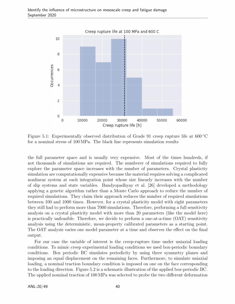
The physically-motivated model describing the creep behavior of Grade 91 has two maincomponents. The prior austenite grain (PAG) model and the grain boundary cavitation(GBC) model. Previous work calibrated the PAG and GBC models to fit the deterministicaverage of a set of Grade 91 experimental [3, 12, 22, 23]. However, a deterministic modelcannot capture the experimentally observed variability in creep-rupture life. Figure 5.1depicts the experimentally observed distribution of Grade 91 creep rupture life at 600 ◦C fora nominal stress of 100 MPa. The black line shows the computed time to creep rupture usingthe calibrated parameters.
Both the PAG and GBC models include the simulated creep curve and rupture life. Asboth models are physically-based, their parameters aim to describe the evolution of mi-crostructural deformation and failure mechanism of Grade 91. The PAG model incorporatestwo different mechanisms: i) point defect diffusion, and ii) dislocation creep. Point defectsdiffusion is related to the chemical potential, enhanced by temperature and driven by stressgradients. The accumulation and flux of point defect results in a measurable strain contribu-tion. The PAG model incorporate point defect diffusion utilizing an isotropic linear diffusionmodel that generates a strain rate proportional to the deviatoric stress and a diffusion coeffi-cient A. Dislocation creep is modeled utilizing a crystal plasticity (CP) approach [24] whichuses a power-law to determine the amount of dislocation glide, and includes a slip resistancestrengthening term to mimic the apparent slip resistance increase observed in experiments[14, 25].
The GBC incorporates three distinct mechanisms: i) cavity growth, ii) cavity nucleation,and iii) grain boundary sliding. These three mechanism are interlaced with each otherthrough a set of coupled rate equations describing the evolution of void nucleation andcavitation. The GBC model assumes continuous nucleation and continuous growth of cavitiesgenerating from carbides present at the grain boundaries. The cavity nucleation rate isgoverned by two parameters: a prefactor FN and a traction normalization value Σ0. Thecavity nucleation rate is modeled via the variable b, which physically represents the half spacebetween two adjacent cavities. The cavity growth process is mathematically expressed interms of the average cavity half radius a, which is geometrically linked to the grain boundaryopening via a geometric relationship. The only three calibrated parameters in this model arethe grain boundary diffusivity DGB, the equilibrium cavity shape angle ΨGB, and the cavitygrowth exponent nGB. Besides the evolution parameters, the GBC model requires the initialnumber of cavities, a0 and the initial cavity spacing b0.
The calibrated parameters will be the baseline for the sensitivity analysis. More detailsabout the PAG and the GBC models, including equations and parameters values, can befound in sections 4.1 and 4.2. Table 4.1 and 4.2 list all the parameters and they calibratedvalues for the PAG and GBC models, respectively.
5.1 Sensitivity analysis
Sensitivity analysis is a well known technique to identify the most sensitive parameters of amodel with respect to a target scalar variable. A full sensitivity analysis requires exploring
ANL-20/49 39
Identify the influence of microstructure on mesoscale creep and fatigue damageSeptember 2020
Figure 5.1: Experimentally observed distribution of Grade 91 creep rupture life at 600 ◦Cfor a nominal stress of 100 MPa. The black line represents simulation results
the full parameter space and is usually very expensive. Most of the times hundreds, ifnot thousands of simulations are required. The numberer of simulations required to fullyexplore the parameter space increases with the number of parameters. Crystal plasticitysimulation are computationally expensive because the material requires solving a complicatednonlinear system at each integration point whose size linearly increases with the numberof slip systems and state variables. Bandyopadhyay et al. [26] developed a methodologyapplying a genetic algorithm rather than a Monte Carlo approach to reduce the number ofrequired simulations. They claim their approach reduces the number of required simulationsbetween 100 and 1000 times. However, for a crystal plasticity model with eight parametersthey still had to perform more than 7000 simulations. Therefore, performing a full sensitivityanalysis on a crystal plasticity model with more than 20 parameters (like the model here)is practically unfeasible. Therefore, we decide to perform a one-at-a-time (OAT) sensitivityanalysis using the deterministic, mean-property calibrated parameters as a starting point.The OAT analysis varies one model parameter at a time and observes the effect on the finaloutput.
For our case the variable of interest is the creep-rupture time under uniaxial loadingconditions. To mimic creep experimental loading conditions we used box-periodic boundaryconditions. Box periodic BC simulates periodicity by using three symmetry planes andimposing an equal displacement on the remaining faces. Furthermore, to simulate uniaxialloading, a nominal traction boundary condition is imposed on one on the face correspondingto the loading direction. Figure 5.2 is a schematic illustration of the applied box-periodic BC.The applied nominal traction of 100 MPa was selected to probe the two different deformation
ANL-20/49 40

Identify the influence of microstructure on mesoscale creep and fatigue damageSeptember 2020
Figure 5.2: Schematic representing box-periodic boundary conditions for uniaxial creep load-ing. The colored block represents the RVE and each color represents a grain. TZ is thenominal traction and corresponds to a constant applied force.
regimes observed for Grade 91 [3, 27]. 100 MPa is the watershed between the diffusional anddislocation bulk grain deformation mechanism. Figure 5.3 depicts simulation results for anapplied nominal traction of 100 MPa.
During experiments, the rupture time can be easily measured as the time until the speci-men breaks in half. However, including failure in stress controlled finite element simulationsis challenging. When damage is widespread the structure will not be able to sustain theimposed load, and the finite element simulation will have difficulty converging, thus requir-ing small time steps, greatly increasing the cost of the simulations. Therefore we define astopping criteria short of complete RVE failure. To examine the impact of this criteria onthe sensitivity analysis, we consider three options:
1. the time to 1 % interface strain (TT1) in the loading direction,
2. the time to 2 % interface strain (TT2) in the loading direction,
3. the time to 3 % interface strain (TT3) in the loading direction.
If the sensitivity analysis provides the same results for all of the specified failure metrics
ANL-20/49 41

Identify the influence of microstructure on mesoscale creep and fatigue damageSeptember 2020
Figure 5.3: Rendering of simulation results for uniaxial creep and a nominal stress of100 MPa.
ANL-20/49 42
Identify the influence of microstructure on mesoscale creep and fatigue damageSeptember 2020
then it can be considered unbiased. The interface strain contribution is computed as:
εGB,ij =
∫AlGB,ijdA
V0
A0
A(5.1)
lGB,ij =JuKinj + niJuKj
2(5.2)
(5.3)
where A and A0 are the deformed and undeformed grain boundary area, V0 is the initialvolume, JuK is the displacement jump, and n is the interface normal in the deformed config-uration.
The OAT analysis is performed by increasing each model parameter by a fix ratio, R =1 · 10−6 and then computing the variation of the outcome as:
S∗p =
∣∣∣∣TT ∗(p(1 +R))− TT ∗(p)pR
∣∣∣∣ (5.4)
where TT ∗ is any of the failure metrics. A few parameters of the PAG and GBC modelsare related to each other. Specifically, the interface Young’s and shear modulus, EGB andGGB, are always assumed to be equal to the bulk material. Furthermore, the grain boundarydiffusivity, DGB and the grain boundary viscosity, ηGB, are assumed to be related by [22, 28]:
ηGB =C
DGB
(5.5)
where C = 1 · 10−9 mm2 is the proportionality constant computed using the calibrateddeterministic values of DGB and ηGB.
Results of the OAT sensitivity analysis are reported in Fig. 5.4. The first noticeablefeature is the independence of the sensitivity from the selected failure metric. This impliesthat any of the three metric is equally good to identify the most relevant model parameters.In what follow we will use the time to 1 % interface strain, TT1, as the failure metric.Furthermore, the results also show that the most sensitive parameter is the grain boundarydiffusivity, DGB. This result is not surprising and confirms that diffusional cavity growth isthe dominant failure mechanism. This also implies that grain boundary viscosity might play arole because the viscosity is related to the diffusivity by Eq. 5.5. The second most influentialparameter among the grain boundary model parameters is the initial cavity half radius, a0,which is related to the size of second phase particle distribution at grain boundaries. TheThe most sensitive parameter for the grain bulk is the point defect diffusivity constantA. The grain bulk diffusivity is responsible for contributing to the total inelastic strainrate (Eq. 4.7), and therefore contributes to the triaxial cavity growth rate (Eq. 4.15).Conversely parameter related to dislocation glide, like, γ0, τ0, τsat, and θ , show a lessereffect on the creep failure time. Their lower effect might be related to the low appliedstress (100 MPa). Furthermore the, small effect of the dislocation creep parameters impliesthat diffusional creep is the dominant deformation mechanisms at this regime. A morecomprehensive sensitivity analysis should be performed to fully investigate the effect of allthe parameters on the creep behavior of Grade 91. A viable and simple approach wouldbe to repeat the above analysis for different nominal traction levels, to identify at least themost sensitive parameter at each level.
ANL-20/49 43

Identify the influence of microstructure on mesoscale creep and fatigue damageSeptember 2020
Figure 5.4: Sensitivity of different failure metrics with respect to the model parameterswhen performing a one-at-a-time sensitivity analysis. The failure metrics are: i) time to 1 %interface strain (TT1), ii) time to 2 % interface strain (TT2), and iii) time to 3 % interfacestrain (TT3). Sensitivity is plotted in log space.
ANL-20/49 44
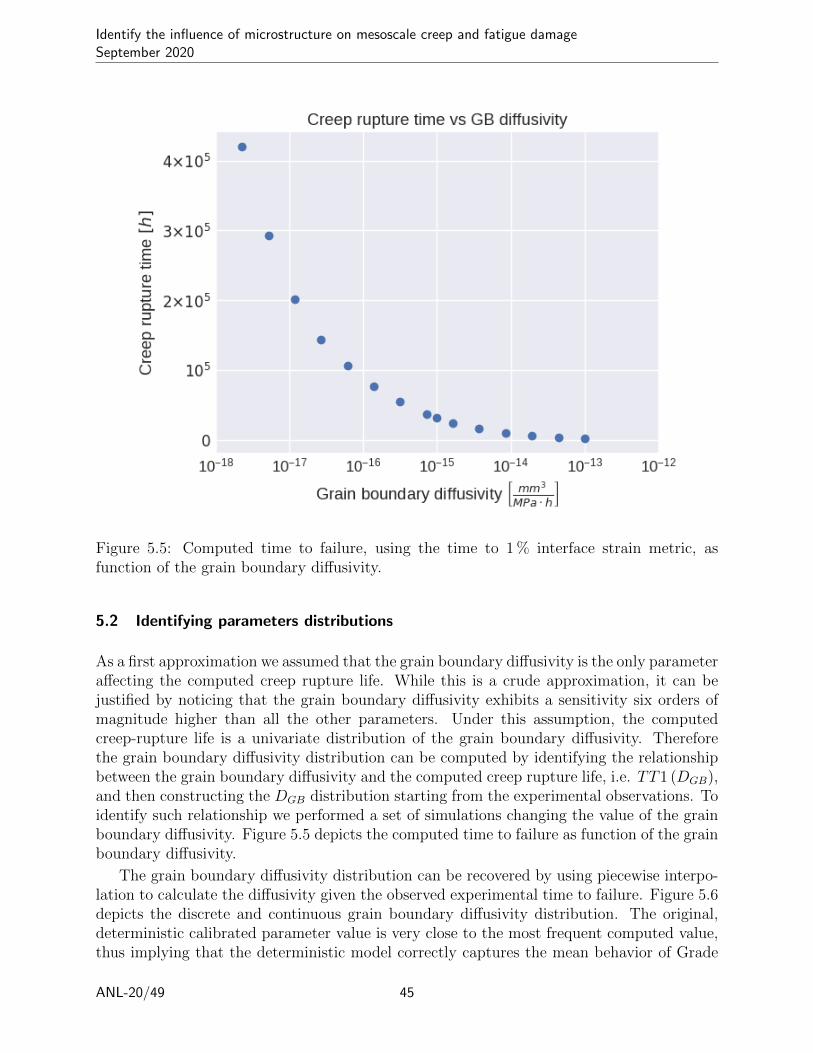
Identify the influence of microstructure on mesoscale creep and fatigue damageSeptember 2020
Figure 5.5: Computed time to failure, using the time to 1 % interface strain metric, asfunction of the grain boundary diffusivity.
5.2 Identifying parameters distributions
As a first approximation we assumed that the grain boundary diffusivity is the only parameteraffecting the computed creep rupture life. While this is a crude approximation, it can bejustified by noticing that the grain boundary diffusivity exhibits a sensitivity six orders ofmagnitude higher than all the other parameters. Under this assumption, the computedcreep-rupture life is a univariate distribution of the grain boundary diffusivity. Thereforethe grain boundary diffusivity distribution can be computed by identifying the relationshipbetween the grain boundary diffusivity and the computed creep rupture life, i.e. TT1 (DGB),and then constructing the DGB distribution starting from the experimental observations. Toidentify such relationship we performed a set of simulations changing the value of the grainboundary diffusivity. Figure 5.5 depicts the computed time to failure as function of the grainboundary diffusivity.
The grain boundary diffusivity distribution can be recovered by using piecewise interpo-lation to calculate the diffusivity given the observed experimental time to failure. Figure 5.6depicts the discrete and continuous grain boundary diffusivity distribution. The original,deterministic calibrated parameter value is very close to the most frequent computed value,thus implying that the deterministic model correctly captures the mean behavior of Grade
ANL-20/49 45

Identify the influence of microstructure on mesoscale creep and fatigue damageSeptember 2020
Figure 5.6: The numerically computed grain boundary diffusivity distribution. Verticalline represent the calibrated DGB value. The blue line represents a smooth distributioncalculated using the kernel density estimation.
91. The width of the diffusivity distribution is approximately three orders of magnitude,which reasonably matches experimental measurements. McGarrity et al. [29] showed thatthe variation of diffusivity between low energy and high energy grain boundaries is approxi-mately 10 orders of magnitude. Cao et al. [30] Showed that the excess free volume is linearlycorrelated to the grain boundary energy. Furthermore, it is reasonable to assume that thegrain boundary diffusivity is linearly related to excess free volume, because a larger free vol-ume would ease the diffusion process. Hence the diffusivity can be assumed to be correlatedto the grain boundary energy. Ratanaphan et al. [31] computed the free surface energy ofmore than 400 grain boundaries, including very low energy and random grain boundaries.Normalizing their results shows that variability of the grain boundary energy for randomgrain boundaries is about 30 % (see Figure 5.7). Hence, by assuming a log-linear correlationbetween the grain boundary diffusivity and the grain boundary energy, a 30 % variability inenergy can explain the 3 orders of magnitude variability on the grain boundary diffusivity .
The other parameters exhibiting high sensitivity should also be incorporated in the modelfor a full sensitivity analysis. Also our analysis does not account for correlations betweendifferent parameters, except for the correlation between diffusivity and sliding viscosity dis-cussed in Section 5.1.
ANL-20/49 46

Identify the influence of microstructure on mesoscale creep and fatigue damageSeptember 2020
Figure 5.7: Normalized grain boundary energy. The dashed line shows the variability of theenergy for random grain boundaries. Data from [31]
ANL-20/49 47

Identify the influence of microstructure on mesoscale creep and fatigue damageSeptember 2020
6 Conclusions and future work
This report includes both improvements to MOOSE framework and a preliminary microstruc-tural model capturing the observed scatter of the creep rupture life of Grade 91.
Improvements to the MOOSE framework include:
• The addition of a large-deformation kernel to the tensor mechanics module allowingMOOSE to use a total Lagrangian formulation. The new kernel also include the ana-lytically correct Jacobian.
• A new scalar kernel system imposing average stress and strain for arbitrarily-shapedunit cells while maintaining the Hill-Mandel condition.
• A new mesh generator that automatically detects periodic boundaries for arbitrarily-shaped unit cells. The mesh generator was designed to allow users to directly utilizeperiodic Voronoi tessellation generated by Neper without utilizing any kind of externalpreprocessing tool.
• A new large-deformation cohesive zone model accounting for large area changes andlarge rotations of the interface. The introduction of a large deformation cohesive zonesystem was necessary to account for the large area changes observed during creep tests.This system includes both a new material and a new kernel. The new system also alsoincludes the analytically correct Jacobian.
All the above improvements together will allow MOOSE users to perform true periodiccrystal plasticity simulations without the need of meshing tools or preprocessing scripts,while utilizing a consistent stress measure. Pull requests to merge all the above improvementsinto MOOSE are in preparation and could be used in future modeling efforts.
The microstructural model for creep in Grade 91 was used to identify key microstructuralparameters controlling creep failure:
• A one-at-a-time sensitivity analysis was performed to identify the parameters mostinfluencing the computed creep-rupture life of Grade 91 at a constant nominal stressof 100 MPa. Results of the sensitivity analysis showed that the most influential modelparameter is the grain boundary diffusivity.
• By using the sensitivity analysis results we showed that the experimentally observedcreep-rupture life scatter can be accounted for utilizing a univariate statistical modelonly including the distribution of the grain boundary diffusivity.
• The obtained grain boundary diffusivity distribution was reasonable because its com-puted variability is comparable to the variability of the grain boundary energies.
While the proposed probabilistic model is able to capture the statistical distribution forcreep-rupture life of Grade 91 steel further validation is need to demonstrate its applicabilityto a wider range of applied stresses.
Furthermore it would be of scientific and engineering interest to include the variabilityof other parameters to better capture the experimentally observed deformation and failurevariability. For instance recent experiments performed at the Advanced Photon Source show
ANL-20/49 49

Identify the influence of microstructure on mesoscale creep and fatigue damageSeptember 2020
that not all the favorably oriented grain boundaries will experience cavitation. This is incontrast with the baseline results of the utilized physically-based micro-mechanical model [4].The most probable cause of this behavior is the homogeneity of grain boundary propertiesin the model. There is experimental evidence [32, 33] and numerical studies [12, 34] showingthat accounting for the grain boundary character greatly increase the predictive capabilityof grain boundary models. Bulatov et al. [35] proposed a methodology computing the grainboundary energy given the grain boundary character, Ratanaphan et al. [31] found correla-tions between the grain boundary energy and grain boundary properties. Incorporating thegrain boundary character in the micro-mechanical model will remove the assumption thatall grain boundaries are equal and will incorporate the inherent grain boundary propertiesvariability observed in experiments.
In addition to this improvement to the model physics, better numerical methods will beneeded for UQ analysis through the CPFEM model. Chapter 5 cites [26], which promisesa significant reduction in computational cost versus a Monte Carlo method. This techniquecould be explored. Additionally, improvements to the model numerics to reduce computationtime will directly translate to reducing the time required for UQ.
Finally, this general approach could be extended to creep-fatigue simulations. The intro-duction notes that the program focused in FY2020 on creep loading, but future work willextend to creep-fatigue. Here, numerical expense will be critical as cyclic loading requireslarge numbers of time steps simply to represent the load reversals. The methods described inthe previous paragraph could be helpful. Additionally, cyclic extrapolation schemes could bedeveloped to skip entire load cycles without significantly compromising the model’s accuracy.
ANL-20/49 50

Identify the influence of microstructure on mesoscale creep and fatigue damageSeptember 2020
Acknowledgements
The research was sponsored by the U.S. Department of Energy, under Contract No. DEAC02-06CH11357 with Argonne National Laboratory, managed and operated by UChicago Ar-gonne LLC. Programmatic direction was provided by the Nuclear Energy Advanced Mod-eling & Simulation Program of the Department of Nuclear Energy. The authors gratefulacknowledge the support and direction of Ben Spencer, at Idaho National Laboratory, Na-tional Technical Director Chris Stanek, at Los Alamos National Laboratory, and FederalManager Dave Henderson.
ANL-20/49 51

Identify the influence of microstructure on mesoscale creep and fatigue damageSeptember 2020
Bibliography
[1] R. W. Swindeman, M. L. Santella, P. J. Maziasz, B. W. Roberts, and K. Coleman.Issues in replacing Cr-Mo steels and stainless steels with 9Cr-1Mo-V steel. InternationalJournal of Pressure Vessels and Piping, 81(6):507–512, 2004. ISSN 03080161. doi:10.1016/j.ijpvp.2003.12.009.
[2] J. R. DiStefano, V. K. Sikka, J. J. Blass, C. R. Brinkman, J. M. Corum, J. A. Horsk,R. L. Huddleston, J. F. King, R. W. McClung, and W. K. Sartory. Summary of Modified9Cr-1Mo Steel Development Program 1975-1985. Technical report, Oak Ridge NationalLaboratory ORNL-6303, 1986.
[3] Omar Nassif, Timothy J. Truster, Ran Ma, Kristine B. Cochran, David M. Parks, M. C.Messner, and T. L. Sham. Combined crystal plasticity and grain boundary modelingof creep in ferritic-martensitic steels: I. Theory and implementation. Modelling andSimulation in Materials Science and Engineering, 27(7), 2019. ISSN 1361651X. doi:10.1088/1361-651X/ab359c.
[4] M. C. Messner, Omar Nassif, Ran Ma, Timothy J. Truster, Kristine Cochran, DavidParks, and T.-L. Sham. Combined crystal plasticity and grain boundary modeling ofcreep in ferritic-martensitic steels: II. The effect of stress and temperature on engineer-ing and microstructural properties. Modelling and Simulation in Materials Science andEngineering, 27:075010, 2019.
[5] Andrea Rovinelli, Henry Proudhon, Ricardo A Lebensohn, and Michael D Sangid. As-sessing the reliability of fast fourier transform-based crystal plasticity simulations of apolycrystalline material near a crack tip. International Journal of Solids and Structures,184:153–166, 2020.
[6] Romain Quey, PR Dawson, and Fabrice Barbe. Large-scale 3d random polycrystals forthe finite element method: Generation, meshing and remeshing. Computer Methods inApplied Mechanics and Engineering, 200(17-20):1729–1745, 2011.
[7] Rodney Hill. Elastic properties of reinforced solids: some theoretical principles. Journalof the Mechanics and Physics of Solids, 11(5):357–372, 1963.
[8] J Mandel. Contribution theorique a l’etude de l’ecrouissage et des lois de l’ecoulementplastique. In Applied Mechanics, pages 502–509. Springer, 1966.
[9] M. Danielsson, D. M. Parks, and M. C. Boyce. Three-dimensional micromechanicalmodeling of voided polymeric materials. Journal of the Mechanics and Physics of Solids,50(2):351–379, 2002. ISSN 00225096. doi: 10.1016/S0022-5096(01)00060-6.
[10] B. S. Kirk, J. W. Peterson, R. H. Stogner, and G. F. Carey. libMesh: A C++ Libraryfor Parallel Adaptive Mesh Refinement/Coarsening Simulations. Engineering with Com-puters, 22(3–4):237–254, 2006. https://doi.org/10.1007/s00366-006-0049-3.
[11] Cody J. Permann, Derek R. Gaston, David Andrs, Robert W. Carlsen, Fande Kong,Alexander D. Lindsay, Jason M. Miller, John W. Peterson, Andrew E. Slaughter, Roy H.
ANL-20/49 53
Identify the influence of microstructure on mesoscale creep and fatigue damageSeptember 2020
Stogner, and Richard C. Martineau. MOOSE: Enabling massively parallel multiphysicssimulation. SoftwareX, 11:100430, 2020. ISSN 2352-7110. doi: https://doi.org/10.1016/j.softx.2020.100430. URL http://www.sciencedirect.com/science/article/
pii/S2352711019302973.
[12] MC Messner, A Rovinelli, DM Parks, and T-L Sham. Evaluation of statistical variationof microstructural properties and temperature effects on creep fracture of grade 91.Technical Report ANL-ART-143, Argonne National Lab.(ANL), Argonne, IL (UnitedStates), Lemont, IL, USA, 2018.
[13] A. Rovinelli, M. C. Messner, Guosheng Ye, and T.-L. Sham. Initial study of notchsensitivity of grade 91 using mechanisms motivated crystal plasticity finite elementmethod. Technical Report ANL-ART-171, Argonne National Laboratory, Lemont, IL,USA, 2020.
[14] Kazuhiro Kimura, Kota Sawada, and Hideaki Kushima. Creep rupture ductility of creepstrength enhanced ferritic steels. Journal of Pressure Vessel Technology, 134(3), 2012.
[15] Vinh Phu Nguyen. An open source program to generate zero-thickness cohesive interfaceelements. Advances in Engineering Software, 74:27–39, 2014.
[16] Vinh Phu Nguyen. Discontinuous galerkin/extrinsic cohesive zone modeling: Imple-mentation caveats and applications in computational fracture mechanics. EngineeringFracture Mechanics, 128:37–68, 2014.
[17] Yi Chao Chen and Lewis Wheeler. Derivatives of the stretch and rotation tensors.Journal of Elasticity, 32(3):175–182, 1993. ISSN 03743535. doi: 10.1007/BF00131659.
[18] Argonne National Laboratory. NEML: the Nuclear Engineering material Model Library.https://github.com/Argonne-National-Laboratory/neml, 2019.
[19] T-L Sham and A Needleman. Effects of triaxial stressing on creep cavitation ofgrain boundaries. Acta Metallurgica, 31(6):919–926, jun 1983. ISSN 00016160. doi:10.1016/0001-6160(83)90120-7. URL https://linkinghub.elsevier.com/retrieve/
pii/0001616083901207.
[20] Erik Van Der Giessen, M W D der Burg, A Needleman, and V Tvergaard. Void growthdue to creep and grain boundary diffusion at high triaxialities. Journal of the Mechanicsand Physics of Solids, 43(1):123–165, 1995. ISSN 00225096. doi: 10.1016/0022-5096(94)00059-E.
[21] A. Rovinelli, M. C. Messner, and T.-L. Sham. Initial microstructural model for creep-fatigue damage in grade 91 steel. Technical Report ANL-ART-202, Argonne NationalLaboratory, Lemont, IL, USA, 2020.
[22] Mark Christian Messner, Omar Nassif, Ran Ma, Timothy J Truster, Kristine Cochran,David Parks, and TL Sham. Combined crystal plasticity and grain boundary modeling ofcreep in ferritic-martensitic steels: Ii. the effect of stress and temperature on engineering
ANL-20/49 54

Identify the influence of microstructure on mesoscale creep and fatigue damageSeptember 2020
and microstructural properties. Modelling and Simulation in Materials Science andEngineering, 27(7):075010, 2019.
[23] M. C. Messner, T. J. Truster, K. B. Cochran, D. M. Parks, and T.-L. Sham. FY17status report on the micromechanical finite element modeling of creep fracture of Grade91 steel. Technical Report ANL-ART-95, Argonne National Laboratory, 2017.
[24] R. J. Asaro. Crystal plasticity. Transactions of the ASME. Journal of Applied Mechan-ics, 50(4B):921–934, 1983.
[25] Kouichi Maruyama, Kota Sawada, and Jun ichi Koike. Strengthening mechanisms ofcreep resistant tempered martensitic steel. ISIJ International, 41(6):641–653, 2001. doi:10.2355/isijinternational.41.641.
[26] Ritwik Bandyopadhyay, Veerappan Prithivirajan, and Michael D Sangid. Uncertaintyquantification in the mechanical response of crystal plasticity simulations. JOM, 71(8):2612–2624, 2019.
[27] Lubos Kloc and Vaclav Sklenicka. Transition from power-law to viscous creep behaviourof p-91 type heat-resistant steel. Materials Science and Engineering: A, 234:962–965,1997.
[28] RC Gifkins and KU Snowden. Mechanism for “viscous” grain-boundary sliding. Nature,212(5065):916–917, 1966.
[29] E. S. McGarrity, P. M. Duxbury, and E. A. Holm. Statistical physics of grain-boundaryengineering. Phys. Rev. E, 71:026102, Feb 2005. doi: 10.1103/PhysRevE.71.026102.URL https://link.aps.org/doi/10.1103/PhysRevE.71.026102.
[30] Fuhua Cao, Yong Jiang, Tao Hu, and Dengfeng Yin. Correlation of grain boundary extrafree volume with vacancy and solute segregation at grain boundaries: a case study for Al.Philosophical Magazine, 98(6):464–483, 2018. ISSN 14786443. doi: 10.1080/14786435.2017.1408968. URL https://doi.org/10.1080/14786435.2017.1408968.
[31] Sutatch Ratanaphan, David L. Olmsted, Vasily V. Bulatov, Elizabeth A. Holm, An-thony D. Rollett, and Gregory S. Rohrer. Grain boundary energies in body-centeredcubic metals. Acta Materialia, 88:346–354, 2015. ISSN 13596454. doi: 10.1016/j.actamat.2015.01.069. URL http://dx.doi.org/10.1016/j.actamat.2015.01.069.
[32] Meimei Li, K. Natesan, and Weiying Chen. Report on understanding and predictingeffects of thermal aging on microstructure and tensile properties of grade 91 steel forstructural components. Technical Report ANL-ART-108, Argonne National Laboratory,8 2017.
[33] MA Linne, A Venkataraman, MD Sangid, and S Daly. Grain boundary sliding and sliptransmission in high purity aluminum. Experimental Mechanics, 59(5):643–658, 2019.
ANL-20/49 55

[34] Ajey Venkataraman, Marissa Linne, Samantha Daly, and Michael D Sangid. Criteriafor the prevalence of grain boundary sliding as a deformation mechanism. Materialia,8:100499, 2019.
[35] Vasily V Bulatov, Bryan W Reed, and Mukul Kumar. Grain boundary energy functionfor fcc metals. Acta Materialia, 65:161–175, 2014.


Applied Materials DivisionArgonne National Laboratory9700 South Cass Avenue, Bldg. 212Argonne, IL 60439
www.anl.gov
Argonne National Laboratory is a U.S. Department of Energylaboratory managed by UChicago Argonne, LLC