Identification of the Workspace Boundary Of a General 3-R ...

Identification of the Workspace Boundary

Of a General 3-R Manipulator

Erika Ottaviano**, Manfred Husty*, Marco Ceccarelli**

**LARM Laboratory of Robotics and Mechatronics

DiMSAT – University of Cassino

Via Di Biasio 43 - 03043 Cassino (Fr), Italy,

E-mail: ottaviano/[email protected]

* Institute for Engineering Mathematics Geometry and

Computer Science – University of Innsbruck

Technikerstr. 13 A-6020 Innsbruck, Austria

E-mail: [email protected]

Keywords: Kinematics, Serial Manipulators, Workspace, Geometric Singularities, Void.

Abstract

In this paper an algebraic formulation is presented for the boundary workspace of 3-R

manipulators in Cartesian Space. It is shown that the cross-section boundary curve can be

described by a 16-th order polynomial as function of radial and axial reaches. The cross-section

boundary curve and workspace boundary surface are fully cyclic. Geometric singularities of the

curve are identified and characterized. Numerical examples are presented to show the usefulness

of the proposed investigation and to classify the design characteristics.

1. Introduction

Workspace and singularity analyses of serial manipulators have been the focus of intense

research in past decades. The computation of the workspace and its boundary is of significant

interest because of their impact on manipulator design, placement in a working environment, and

trajectory planning.

Most of the industrial manipulators are wrist-partitioned, that is a concatenation of a 3-R

(Revolute) arm, i.e., regional structure, and a spherical wrist attached to the terminal link of the

arm. The workspace analysis of such manipulator can be performed by considering the

Paper MD 04-1384 Ottaviano 1

positioning and orienting singularities separately.

Early studies on the subject were developed in (Roth 1975). The relationship between kinematic

geometry and manipulator performances has been formulated in (Kumar and Waldron 1981).

Gupta and Roth analyzed the effect of hand size on workspace in (Gupta and Roth 1982). An

algorithm for the workspace determination of a general N-R robot has been developed in (Tsai

and Soni 1983). An algebraic formulation for determining the workspace of 3-R manipulators

has been presented in (Ceccarelli 1989) and then generalized for N-R manipulators in (Ceccarelli

1996). Furthermore, the proposed formulation has been used for design purposes in (Ceccarelli

1995), and optimal design procedure in (Lanni et al. 2002; Ceccarelli and Lanni 2004).

Numerical criteria to analyze the workspace of a general multi-degree-of-freedom (DOF) system

has been formulated in (Haug et al. 1994), based on the study of a row-rank deficiency of its

Jacobian. Most of the work has been done on 3-R manipulators for either positioning

(Freudenstein and Primrose 1984; Spanos and Kohli 1985), or orienting tasks (Angeles 1988).

The determination of the workspace boundary in Cartesian Space has been attempted also in

(Spanos and Kohli 1985; Hsu and Kohli 1987; Smith and Lipkin 1993; Ranjbaran et al. 1992). In

(Ceccarelli and Vinciguerra 1995) an analysis of the workspace boundary of 4-R serial

manipulator has been studied by employing toroidal geometries and providing algebraic

expression. Other papers are related to the singularity of the Jacobian matrix that is usually

expressed in the Joint-Coordinate Space. Regions that are free of singularities in the Joint Space

have been named C-sheets, (Burdick 1995). In C-sheets it is possible to change posture without

passing through singularities (Parenti-Castelli and Innocenti 1988). Manipulators that can change

posture without meeting a singularity have been named cuspidal manipulators in (Wenger, 2000)

because of the existence of cusps in their workspace.

A method has been introduced in (Wenger 1992) to obtain the separating surfaces. Manipulators

that can change posture without meeting a singularity have been named cuspidal manipulators in

(Wenger, 2000). A formulation to obtain the boundary of all surfaces enveloping the workspace


for general 3-DOF mechanisms was discussed in (Abdel-Malek and Yeh 1997), although it was

already proposed in (Ceccarelli 1989). A formulation has been introduced in (Abdel-Malek and

Yeh 1997), for the determination of voids in the workspace of serial manipulators. Furthermore,

it has been shown in (Wenger 2000) how to take into account in the design stage the possibility

for a manipulator to execute non-singular changing posture motions.

Although there are many reports in the field of the workspace analysis, there are still open

problems in the characterization of the workspace boundary. It is of practical interest to detect

the presence of a void in the workspace, since it is a region of unreachable points for the end-

effector of the manipulator. A ring void is a void that is buried within the workspace volume and

has ring topology, (Ceccarelli 1996). The presence of cusps and void can be detected by

analyzing the geometric singularities of the cross-section boundary curve (Ottaviano et al. 1999).

By analyzing the workspace boundary it has been found that four types of ring voids and eight

types of internal branch envelopes may exist. A preliminary classification of ring void types and

geometric singularities has been presented in (Ottaviano et al. 1999). Analysis of cusps in the

workspace boundary has been proposed also in (Burdick, 1995; Saramago et al., 2002).

The analysis of the internal branch of the cross-section boundary curve leads to a classification to

characterize the i-solution region (i=0,2,4) for the Inverse Kinematics Problem (IKP).

Furthermore, it is of practical interest exploring the possibility of changing posture without

meeting a singularity (Parenti-Castelli and Innocenti 1988). A manipulator is said to change

posture if it goes from one inverse kinematic solution to another (Wenger 1992). Changing

posture can be desired for obstacle avoidance or to take into account joint limits. Usually, a non-

redundant manipulator crosses a singularity when changing posture. A class of manipulator can

change posture without meeting a singularity. 3-R manipulators have at most 4 Inverse

Kinematic solutions in their workspace. In general, the number of solutions of the IKP varies

from one point to another in the workspace, which may include regions with 0, 2, or 4 solutions

(Ceccarelli 1995; Wenger 1998). Indeed, a 3R manipulator can be classified as binary or


quaternary, i.e. it may have at most 2 solutions for the IKP, or at most 4 solutions for the IKP

(Wenger et al. 2005).

The presence of cusps and void can be detected by analyzing singular points of the curve

describing the boundary. Preliminary analyses of geometric singularities of the cross-section

boundary curve have been carried out in (Saramago et al. 2002), but to the authors’ knowledge in

the literature there is not an investigation on singular points of the boundary curve for a general

3-R manipulator. A classification of the singularities for a special class of 3-R manipulator is

reported in (Wenger et al. 2005).

The proposed analysis of geometric singularities of a general 3-R manipulator can provide useful

tools in the design stage or use. Singular points of the cross-section curve describing the

boundary workspace are named characteristic points.

In this paper a Cartesian representation of the workspace boundary of a general 3-R manipulator

is presented. Geometric singularities have been determined and used to classify the workspace

boundary of the manipulator, and detect the presence of a void. The curve describing the

workspace boundary gives also useful information for characterization in Cartesian Space of the

i-solution regions (i=0,2,4) for the IKP. Furthermore, the proposed analysis can be used for

design purposes and calculation of the workspace volume of the manipulator.

2. An Algebraic Formulation for the Workspace Boundary of 3R Manipulators

A general 3-R manipulator is sketched in Fig.1, in which the kinematic parameters are denoted

by the standard Hartenberg and Denavit (H-D) notation. Without loss of generality the base

frame is assumed to be coincident with X1Y1Z1 frame when θ1= 0, a0=0 and d1=0. End-effector

point H is placed on the X3 axis at a distance a3 from O3, as shown in Fig.1. The general 3R

manipulator is described by the H-D parameters a1, a2, d2, d3, α1 and α2, and θi, for (i = 1,…,3),

as shown in Fig.1. r is the radial distance of point H from the Z1-axis and z is the axial reach;

both can be expressed as function of H-D parameters.


Figure1. Kinematic scheme of a 3R manipulator.

The position workspace of the 3R manipulator can be obtained by a θ1 rotation of the generating

torus that is traced by H by full revolution of θ2 and θ3.

Alternatively, the boundary of the position workspace can be determined by considering the

envelope surface of the torus family that is traced as function of θ3, when a torus of the family is

obtained by full revolution of θ1 and θ2, as outlined in (Ceccarelli 1989, and 1996). In this case,

the equation of the workspace boundary of point H can be expressed in the cross-section plane

R-Z of the base frame when α1≠0, C≠0 and E≠0, in the form of so-called ring equation

(Ceccarelli 1989, 1996),

CD

CKQL

z2/1

−±−

= , 2/1

2

EFG D)z(C

zAr = ⎥⎦⎤

⎢⎣⎡ ++

+− (1)

in which A, B, C, D, E, F and G are named as architecture coefficients.

The sign ambiguity in z expression can be solved to give two envelope branches that together


give the envelope of the torus family.

Architecture coefficients are function of H-D parameters in the form

( ) 2222

21 dzraA +++= , , 2

22 ra4B −=

1

1

sa2

Cα

= , ( )1

1221 s

cdza2D

αα

+−=

( )322323 csdsaa2E θα+θ−= , ( )( )32232

233332321 cscdscsasaaa4F θαα−αθθ+θ= (2)

1

12331

scscaa2

Gα

ααθ= , , , FGL = 22 EGK += ( )222 BEFKLQ +−=

in which

( ) ( )223233

22332 sdcsaacar α+αθ++θ= , 233232 ssacdz αθ−α= (3)

The cross-section boundary curve f of the 3-R manipulator workspace in R-Z plane can be

thought as the envelope of the θ3-family curves.

A generating torus of the enveloping θ3-family can be expressed as

( ) ( ) 0BDCzAzr 2222 =+++−+ (4)

In order to obtain a closed-form expression in r and z coordinates from the ring equation (1), one

can manipulate Eq. (4) by performing the half-tangent substitution u= tan (θ3/2) in the form

0kukukukuk 012

23

34

4 =++++ (5)

Parameters ki (i = 0,…,4) of Eq. (5) are functions of the H-D parameters, z and r. They can be

expressed in the form


zKzrKzKzKKrKrKk 1iZ22

2Z2iR2

2iZ4

4iZ0iR2

2iR4

4iRi ++++++= (6)

As the coefficients ki are functions of the r and z parameters, Eq. (5) represents a one-parameter

family of curves. The envelope of this family is obtained by eliminating u from Eq. (5) and its

derivatives with respect u. This yields to the function f expressing the cross-section boundary

curve in the form

( ) (∑ ∑= =

+++=8

0i

7

0j

j22jb

i22i zrzczrcf ) (7)

Coefficients ci and cbj are non-linear expressions of the H-D parameters and can be obtained by

KiRj KiRjZj and KiZj coefficients in Eq. (6) together with Eqs. (2-3). For example, c8 coefficient

can be expressed as

( ) ( )42

81

41

438 ssaa536,65c αα= (8)

Equation (7) represents the Cartesian expression in R-Z coordinates for the cross-section

boundary curve for a general 3-R manipulator. Its expression is function of the H-D parameters

through ci and cbj coefficients. This expression can be used to characterize the workspace

boundary better than using Eq. (1).

3. Characteristics of the Cross-Section Boundary Curve

The cross-section boundary curve f in Eq. (7) is fully cyclic and of 16-th degree; it has 2 singular

points at infinity with multiplicity 8 each, that are the 2 circle points. A curve that has the

imaginary circular points as double, triple, points is said to have circularity 2, 3, (Hunt 1978;


Naas at al. 1974). Therefore, the cross-section boundary curve has circularity 8.

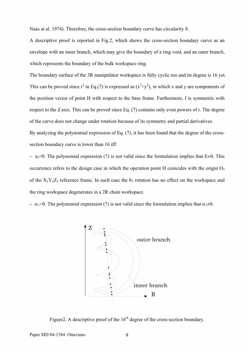
A descriptive proof is reported in Fig.2, which shows the cross-section boundary curve as an

envelope with an inner branch, which may give the boundary of a ring void, and an outer branch,

which represents the boundary of the bulk workspace ring.

The boundary surface of the 3R manipulator workspace is fully cyclic too and its degree is 16 yet.

This can be proved since r2 in Eq.(7) is expressed as (x2+y2), in which x and y are components of

the position vector of point H with respect to the base frame. Furthermore, f is symmetric with

respect to the Z axis. This can be proved since Eq. (7) contains only even powers of r. The degree

of the curve does not change under rotation because of its symmetry and partial derivatives.

By analyzing the polynomial expression of Eq. (7), it has been found that the degree of the cross-

section boundary curve is lower than 16 iff:

− a3=0. The polynomial expression (7) is not valid since the formulation implies that Ε≠0. This

occurrence refers to the design case in which the operation point H coincides with the origin O3

of the X3Y3Z3 reference frame. In such case the θ3 rotation has no effect on the workspace and

the ring workspace degenerates in a 2R chain workspace.

− α1=0. The polynomial expression (7) is not valid since the formulation implies that α1≠0.

Figure2. A descriptive proof of the 16th degree of the cross-section boundary.


− α2=0. This occurrence refers to the design case in which Z2 and Z3 axes are parallel. The

outcome of a Maple computation is that the cross-section boundary curve is of degree 12.

- a1=0. The polynomial expression (7) is not valid since the formulation implies that C≠0.

By analyzing Eq. (8) one can also note that c8 coefficient, that gives the full degree of the curve,

does not depend on a2, d2 and d3 parameters.

4. A Classification of the Geometric Singularities

In general, a singularity is a point at which an equation, curve, or surface, becomes degenerate.

Singularities are often also called singular points or geometric singularities (Gibson, 1998).

Singularities are extremely important in complex analysis, because they characterize all possible

behaviors of analytic functions. Complex singularities are points in the domain of a function

where the function fails to be analytic. Isolated singularities may be classified as poles, essential

singularities, logarithmic singularities, or removable singularities. Non-isolated singularities may

arise as natural boundaries or branch cuts.

Real geometric singularities of the cross-section boundary curve f can be found by introducing

the homogeneous coordinate w in Eq. (7). Thus, one can consider this new equation, which is

function of r, z and w, together with its partial derivatives fr fz and fw with respect to r, z, and w,

respectively.

The zeros of the set of equations: f = 0; fr = 0; fz = 0; and fw = 0 gives the geometric singularities

of the cross-section boundary curve f. Points belonging to these zeros are denoted by Ci, Di, and

Ai where Ci indicates cusps, Di double points and Ai acnodes, referring to a geometric

interpretation that is shown in Fig. 3. They can be classified by considering the second partial

derivatives of f in the form (Gibson, 1998)

zzrr2rz fffg −= (9)


http://mathworld.wolfram.com/Degenerate.html

http://mathworld.wolfram.com/ComplexAnalysis.html

http://mathworld.wolfram.com/Domain.html

http://mathworld.wolfram.com/Function.html

http://mathworld.wolfram.com/AnalyticFunction.html

http://mathworld.wolfram.com/IsolatedSingularity.html

http://mathworld.wolfram.com/Pole.html

http://mathworld.wolfram.com/EssentialSingularity.html

http://mathworld.wolfram.com/EssentialSingularity.html

http://mathworld.wolfram.com/LogarithmicSingularity.html

http://mathworld.wolfram.com/RemovableSingularity.html

http://mathworld.wolfram.com/NaturalBoundary.html

http://mathworld.wolfram.com/BranchCut.html

a) b) c)

Figure 3. The generating manifold for the workspace with characteristic points:

a) a general case; b) a cuspidal manipulator; c) manipulator with double points but no void.

Functions g, fr, fz, and fw can be useful to fully characterize real geometric singularities in the

workspace of the 3R manipulators.

A point Di, whose coordinates are (rdi,zdi), is a double point iff Eq. (9) is greater than zero. A

point Ci, whose coordinates are (rci,zci), is a cusp iff Eq. (9) is equal to zero. A point Ai, whose

coordinates are (rai,zai), is an acnode iff Eq. (9) is less than zero.

A condition on Eq. (9) is useful to characterize the cross-section boundary curve and ring void of

the workspace of 3R manipulators through the points whose geometrical classification is shown

in Fig. 3.

The relationships between the number of singularities of planar algebraic curves is given by the

Pucker’s equations (Husty et al. 1997) whose counting can be expressed in the form

κ−δ−−= 32)1n(nm

ι−τ−−=κ 86)2m(m3 (10)

ι−τ−−= 32)1m(mn

κ−τ−−= 86)2n(n3i


where m is the class, n the curve order, δ the number of ordinary double points, κ the number of

cusps, ι the number of stationary tangents (inflection points), and τ the number of bi-tangents.

Only three of (10) are linearly independent. Equations (10) can give a complete classification of

all singular points of the cross-section boundary curve in Eq. (7).

A point Di is an ordinary double point if its pre-image under f consists of two values and the two

tangent vectors are non-collinear. Geometrically, the meaning is that in a neighborhood of Di, the

curve consists of two transverse branches, as shown in Fig.3a).

A cusp point Ci is a point at which two branches of a curve meet such that the tangents of each

branch are equal, as shown in Fig.3b). An inflection point is a point on a curve at which the sign

of the curvature (i.e., the concavity) changes. A bi-tangent is a line that is tangent to a curve at

two distinct points. An isolated point on a curve Ai, also known as an acnode or hermit point is a

point which has no other points in its neighborhood. Furthermore, the cross-section boundary

curve, as composed by internal and external branches, can be classified into two classes: with

intersecting and non-intersecting branches. For the second class a classification of possible types

of ring void has been presented in a preliminary view in (Ottaviano et al., 1999), in which it has

been pointed out the presence and importance of double points in the cross-section boundary

curve. Examples in Fig. 3 explain the topology of the possible types of internal branches that are

reported as a complete classification in Fig. 4. Geometric singularities of the cross-section

boundary curve can be identified as double points Di, acnodes Ai and cusp points Ci. Internal

branch of the boundary envelope curve in the cross section in R-Z shows generally three loops.

The middle loop can delimit the ring void or a 4-solution region and it is a part of the boundary

curve as pointed out in (Ceccarelli 1989); the others are related to 4-solution regions for the

Inverse Kinematics problem. A ring void can be characterized by the presence of double points,

which have been named as D1 and D2 in Fig. 3. Points D1 and D2 are double points, i.e.

intersections of the inner branch. If there are no double points but there are cusps there is not a

void inside the workspace. In this case, the manipulator belongs to the class of the cuspidal


http://mathworld.wolfram.com/Class.html

http://mathworld.wolfram.com/CurveOrder.html

http://mathworld.wolfram.com/OrdinaryDoublePoint.html

http://mathworld.wolfram.com/Cusp.html

http://mathworld.wolfram.com/StationaryTangent.html

http://mathworld.wolfram.com/InflectionPoint.html

http://mathworld.wolfram.com/Bitangent.html

http://mathworld.wolfram.com/LinearlyDependentFunctions.html

http://mathworld.wolfram.com/Preimage.html

http://mathworld.wolfram.com/TangentVector.html

http://mathworld.wolfram.com/Neighborhood.html

http://mathworld.wolfram.com/Sign.html

http://mathworld.wolfram.com/Curvature.html

http://mathworld.wolfram.com/Line.html

http://mathworld.wolfram.com/TangentLine.html

http://mathworld.wolfram.com/Acnode.html

http://mathworld.wolfram.com/Neighborhood.html

manipulators, Fig.3b). Double points may indicate the presence of a void that corresponds to a 0-

solution region for the Inverse Kinematics problem. Cusp points C1 to C4 can be considered

characteristic points for the cross-section boundary curve since they delimit workspace regions

with multiple configuration reachability. The presence of double points and acnodes, as shown in

Fig. 4, indicates the presence of 4 solution regions for the Inverse Kinematic problem. Acnodes

in Fig. 4 denote the presence of regions with 4-solutions for the IKP. Manipulators with acnodes

present only 2 types of regions: 2 and 4 solution regions. Figure 4 shows a classification in

which there are inner branches that give a ring void and inner branches that indicates the

presence of 4-solution region for the Inverse Kinematic problem. Regions can be suitably

classified by considering a check on the number of possible solutions for the IKP.

Figure 4. Manifolds for inner branches of the workspace boundary envelope of 3R manipulators.

5. Numerical examples

Numerical examples are reported to show most significant cases in the classification of Fig. 4.


Geometric singularities have been determined for all the reported examples as zeros set of

equations: f = 0; fr = 0; fz = 0; and fw = 0; and classified through Eq. (9). It is worth to note that

singular point coordinates will be reported with few decimals, but for their determination and

classification 50 digits have been used in Maple computation.

Figure 5a) shows the cross-section boundary curve of a general case like in Fig. 3. The inner

loop is characterized by the presence of 2 double points and represents a void. Other 2 loops that

are characterized by the cusps are reachable regions of the workspace. Figure5b) shows a plot of

the boundary curve together with f derivatives. It is possible to observe that the derivatives fr, fz,

and fw of the cross-section boundary curve meet at the three singular points D1, C1 and C2. Their

coordinates can be computed as the zeros of the set of the f derivatives. Their coordinates are:

D1=[3.82, 6.62]; C1=[1.87, 7.12]; C2=[3.09, 7.16]. The nature of those characteristic points has

been checked by Eq. (9). It has been verified that C1 and C2 are cusps, since g is equal to zero,

and D1 is a double point, since g is greater than zero.

a) b)

Figure 5. A numerical example for a 3R manipulator with a1=1u; a2=1u; a3=1u; d2=3u; d3=5u;

α1=π/4; α2=π/4: a) cross-section boundary curve f and curves of the 1-parameter family; b) f, fr ,

fz, fw plots. (u is the unit length, and angles are expressed in radians)


In Fig.6 the workspace boundary of a cuspidal manipulator is shown. Points C1=[1.87, 4.13];

C2=[2.99, 4.25], C3=[4.36, 2.07]; C4=[4.38, 2.89] have been checked through Eq. (9).

Figure 7 shows a numerical example in which the cross-section boundary curve f contains only

even powers of r and z. The cross-section boundary curve is of 16th order. There are no cusps nor

double points, no voids, but the internal envelope branch individuates 4-solution region only.

Points A=[1.21, 0.00] and A2=[1.36, 0.00] are acnodes, since g is less than zero. The manipulator

in the numerical example of Fig. 7 is a quaternary manipulator (Wenger et al. 2005).

Figure 8 shows a numerical example in which the cross-section boundary curve has not only

even powers of z. Coordinates of the three singular points on the inner branch are: C1=[1.28,

0.09]; A1=[3.35, 2.5]; C2=[4.60, 0.36]. By evaluating Eq.(9) at points C1, C2 and A1 it has been

verified that C1 and C2 are cusps, since the function g is equal to zero, and A1 is an acnode, since

g is less than zero. Therefore, the presence of an acnode on the inner branch denotes the

existence of a 4-solution region for the Inverse Kinematic problem.

a) b)


α1=π/4; α2=π/4: a) cross-section boundary curve f and curves of the 1-parameter family; b) f, fr,

fz, fw plots.(u is the unit length, and angles are expressed in radians)


a) b)

Figure 7. A numerical example for a 3R manipulator with a1=1u; a2=0.5u; a3=0.8u; d2=0.2u;

d3=0; α1=-π/2; α2=π/2: a) cross-section boundary curve f and curves of the 1-parameter family;

b) f, fr , fz, fw plots. (u is the unit length, angles are expressed in radians)

a) b)


α1=-π/6; α2=π/3: a) cross-section boundary curve f and curves of the 1-parameter family; b) f, fr,

fz, fw plots. (u is the unit length, angles are expressed in radians)


Figure 9 shows a numerical example in which the algebraic expression of the boundary curve has

the degree of 16. The computation shows that the cross-section boundary curve does not contain

singular points, as it is shown in Fig. 9b) in which fr, fz and fw do not intersect. The manipulator

is a binary manipulator (Wenger et al. 2005) since the presence of 2 solution region for the IKP.

The numerical example of Fig. 10 shows that the cross-section boundary curve has only even

powers of r and z and the degree of the curve is 16. Singular points have coordinates: A1=[0.97,

0.00]; D1=[5.73, 0.00]; C1=[6.87, -3.72]; C2=[6.87, 3.72]. A1 has g less than zero (acnode), D1

has g grater than zero (double point) and C1 and C2 have g equal to zero (cusps). It is worth to

note that in this case internal branches delimit two 4-solution regions for the IKP.

Numerical example of Fig. 11 shows a cross-section boundary curve of 16th degree. Singular

points that have been checked are C1=[1.64, 2.77]; D1=[1.85, 2.56]; C2=[1.11, 2.70] and

A1=[3.03, 1.51]. It can be proved that C1 and C2 are cusps, since function g at those points has

value equal to zero.

a) b)


d3=0.5; α1=π/3; α2=π/6: a) cross-section boundary curve f and curves of the 1-parameter family;

b) f, fr, fz, fw plots. (u is the unit length, angles are expressed in radians)


a) b)

Figure 10. A numerical example for a 3R manipulator with a1=1u; a2=3u; a3=4u; d2=3u; d3=0;



a) b)





Point D1 is a double point since it has g greater than zero and A1 is an acnode, since g is less than

zero. It indicates the presence of a void. The inner branch of the cross-section boundary curve

delimits a void and one 4-solution region for the IKP.

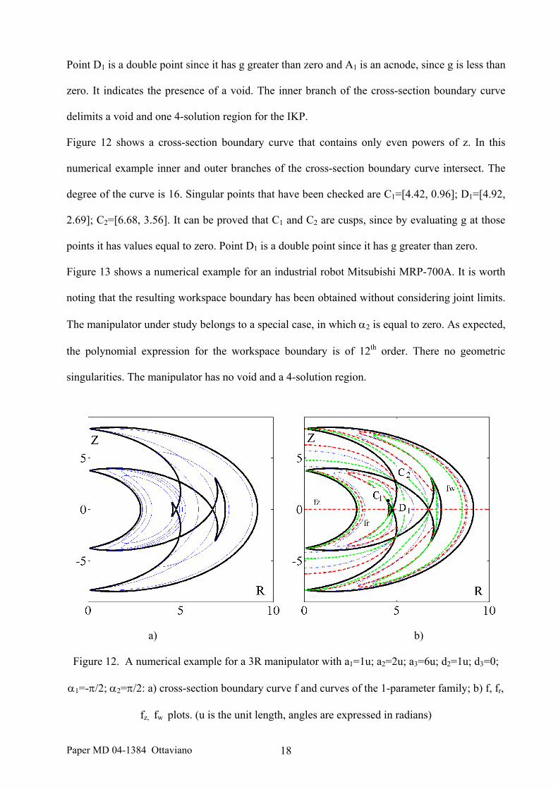
Figure 12 shows a cross-section boundary curve that contains only even powers of z. In this

numerical example inner and outer branches of the cross-section boundary curve intersect. The

degree of the curve is 16. Singular points that have been checked are C1=[4.42, 0.96]; D1=[4.92,

2.69]; C2=[6.68, 3.56]. It can be proved that C1 and C2 are cusps, since by evaluating g at those

points it has values equal to zero. Point D1 is a double point since it has g greater than zero.

Figure 13 shows a numerical example for an industrial robot Mitsubishi MRP-700A. It is worth

noting that the resulting workspace boundary has been obtained without considering joint limits.

The manipulator under study belongs to a special case, in which α2 is equal to zero. As expected,

the polynomial expression for the workspace boundary is of 12th order. There no geometric

singularities. The manipulator has no void and a 4-solution region.

a) b)





a) b)

Figure 13. A numerical example for Mitsubishi MRP-700A manipulator with a1=250; a2=1000;

a3=1209; d2=0; d3=0; α1=π/2; α2=0: a) cross-section boundary curve f and curves of the 1-

parameter family; b) f, fr, fz, fw plots. (lengths are expressed in mm, angles are expressed in

radians)

6. Conclusion

An algebraic formulation has been presented for a Cartesian representation of the workspace

boundary of a general 3-R manipulator. In particular, with the formulation derived in this paper it

is possible to apply the vast geometric literature on algebraic curves to workspace analysis. It has

been found that the cross-section boundary curve and boundary surface are of 16-th degree and

fully cyclic. Furthermore, a formulation has been presented to identify all geometric singularities

of the cross-section boundary curve. Geometric singularities of the cross-section boundary curve

are identified as double points, cusps and acnodes, and classified as delimiting ring void and 4-

solution regions. Numerical examples have been presented to outline the practical feasibility of

the proposed formulation but mainly for a characterization of the manifolds for the inner branch

of the workspace boundary envelope. In particular, it is possible to characterize the workspace

by analyzing inner braches delimiting 2-solution regions and 4-solution regions for the IKP.


Furthermore, the proposed analysis can be useful for design purposes and to deduce an

evaluation of the workspace volume by integrating the boundary curve.

References

Abdel-Malek K., Yeh H-J., 1997, “Analytical Boundary of the Workspace for General 3-DOF

Mechanisms”, The International Journal of Robotics Research, Vol. 16, No.2, pp. 198-213.

Abdel-Malek K., Yeh H-J., Othman S., 2000, “Understanding Voids in the Workspace of Serial

Robot Manipulators”, ASME DETC 2000 Biennial Mechanism Conference, Baltimore.

Angeles J., 1988, “Special Loci of the Workspace Spherical Wrists”, Proceedings of the First

International Workshop on Advances in Robotics Kinematics, Ljubljana, pp. 36-45.

Bruce, J. W., Giblin, P. J., 1992, “Curves and Singularities: A Geometrical Introduction to

Singularity Theory”, Cambridge University Press, 2nd Edition.

Burdick, J. W., 1995, “A Classification of 3R Regional Manipulator Singularities and

Geometries”, Mechanism and Machine Theory, Vol. 30, No.1, pp. 71-89.

Ceccarelli M., 1989, “On the Workspace of 3R Robot Arms”, Proceedings of the Fifth IFToMM

International Symposium on Theory and Practice of Mechanism, Bucharest, Vol. II-1, pp.

37-46.

Ceccarelli M., 1996, “A Formulation for the Workspace Boundary of General N-Revolute

Manipulators”, Mechanisms and Machine Theory, Vol.31, No.5, pp. 637-646.

Ceccarelli M., Vinciguerra A., 1995, “On the Workspace of General 4R Manipulators”, The

International Journal of Robotics Research, Vol.14, No.2, pp. 152-160.

Ceccarelli M., Lanni C., 2004, “A Multi-Objective Optimum Design of General 3R Manipulators

for Prescribed Workspace Limits”, Mechanism and Machine Theory, Vol. 39, pp. 119-132.

Freudenstein F., Primrose E.J.F., 1984, “On the Analysis and Synthesis of the Workspace of a

Three-Link, Turning-Pair Connected Robot Arm”, ASME Journal of Mechanisms,

Transmissions and Automation in Design, Vol.106, pp. 365-370.


Gibson C.G., 1998, “Elementary Geometry of Algebraic Curves”, Cambridge University Press.

Gupta K. C., 1986, “On the Nature of Robot Workspace”, The International Journal of Robotics

Research, Vol.5, No.2, pp. 112-121.

Gupta, K. C., Roth, B., 1982, “Design Considerations for Manipulator Workspace”, ASME

Journal of Mechanical Design, Vol. 104, pp. 704-711.

Haug E. J., Adkins R., Luh C. M., 1994, “Numerical Algorithms for Mapping Boundaries of

Manipulator Workspaces”, Proc. 23rd ASME Mechanisms Conference, Minneapolis.

Hayes M.J.D., Husty M.L., Zsombor-Murray P.J., 2002, “Singular Configurations of Wrist-

Partitioned 6R Serial Robots: A Geometric Perspective for Users”, CSME Transactions, Vol.

26, No. 1, 41-55.

Hsu M.S., Kohli D., 1987, “Boundary Surfaces and Accessibility Regions for Regional

Structures of Manipulators”, Mechanism and Machine Theory, Vol.22, No.3, pp. 277-289.

Hunt K.H., “Kinematic geometry”, Clarendon Press, Oxford, 1978.

Husty M., Karger A., Sachs H., Steinhilper W., “Kinematik und Robotik“, Springer Verlag, 1997.

Kumar A., Waldron K.J., 1981, “The Workspace of a Mechanical Manipulator”, ASME Journal

of Mechanical Design, Vol.103, pp. 665-672.

Lanni C., Saramago S., Ceccarelli M., 2002, "Optimum Design of General 3R Manipulators by

Using Traditional and Random Search Optimization Techniques", Journal of the Brazilian

Society of Mechanical Sciences, Vol. XXIV, n.4, pp.293-301.

Naas J., Schmidt H.L., “Mathematisches Wörterbuch“, Band II, Akademieverlag Berlin-Teubner

Verlag Stuttgart, 1974.

Parenti-Castelli V., Innocenti C., 1988, “Position Analysis of Robot Manipulators: Regions and

Sub-Regions”, Proceedings of the First International Conference on Advances in Robot

Kinematics, Ljubljana, pp.150-158.

Ranjbaran F., Angeles J., Patel R.V., 1992, “The Determination of the Cartesian Workspace of

General Three-Axes Manipulators”, Proceedings of the Third International Workshop on


Advances in Robotics Kinematics, Ferrara, pp. 318-325.

Ottaviano E., Ceccarelli M., Lanni C., 1999, “A Characterization of Ring Void in Workspace of

Three-Revolute Manipulators”, Proceedings of the Tenth World Congress on the Theory of

Machines and Mechanisms, Oulu, Vol.3, pp. 1039-1044.

Ottaviano E., Husty M., Ceccarelli M., 2004, “A Cartesian Representation for the Boundary

Workspace of 3R Manipulators”, Advances in Robot Kinematics, Ed. Kluwer Academic

Publishers, Sestri Levante, pp. 247-254.

Roth B., 1975, “Performance Evaluation of Manipulators from a Kinematic Viewpoint”,

National Bureau of Standards Special Publication, No. 459, pp. 39-61.

Tsai Y.C., Soni A.H., 1983, “An Algorithm for the Workspace of a General n-R Robot”, Journal

of Mechanisms, Transmission and Automation in Design, Vol.105, pp. 70-78.

Saramago S., Ottaviano E., Ceccarelli M., 2002, “A Characterization of the Workspace

Boundary of Three-Revolute Manipulators”, Proceedings of DETC’02 ASME 2002 Biennial

Robotics Conference, Montreal, 2002 , paper DETC2002/MECH-34342.

Smith D.R., 1990, “Design of Solvable 6R Manipulators”, Ph.D. Thesis, Georgia Institute of

Technology, Atlanta.

Smith D.R., Lipkin H., 1993, “Higher Order Singularities of Regional Manipulators”,

Proceedings of the IEEE International Conference on Robotics and Automation, Vol.1, pp.

194-199.

Spanos J., Kohli D., 1985, “Workspace Analysis of Regional Structures of Manipulators”,

ASME Journal of Mechanisms, Transmission and Automation in Design, Vol.107, pp. 216-

222.

Wenger P., 1992, “A New General Formalism for the Kinematic Analysis of all Nonredundant

Manipulators”, ”, Proc. IEEE International Conference on Robotics and Automation, Nice,

Vol.1, pp. 442-447.

Wenger P., 2000, ”Some Guidelines for the Kinematic Design of New Manipulators”,


Mechanisms and Machine Theory, Vol.35, No.3, pp.437-449.

Wenger P., Chablat D., Baili M., 2005, “A DH Parameter Based Condition for 3R Orthogonal

Manipulators to Have Four Distinct Inverse Kinematic Solutions”, ASME Journal of

Mechanical Design, ,Vol.127, No.1, pp 150-155.


List of Figure Captions

Figure1. Kinematic scheme of a 3R manipulator.

Figure2. A descriptive proof of the 16th degree of the cross-section boundary.

Figure 3. The generating manifold for the workspace with characteristic points:

a general case; b) a cuspidal manipulator; c) manipulator with double points but no void.

Figure 4. Manifolds for inner branches of the workspace boundary envelope of 3R manipulators.


α1=π/4; α2=π/4: a) cross-section boundary curve f and curves of the 1-parameter family; b) f, fr ,

fz, fw plots. (u is the unit length, and angles are expressed in radians)


α1=π/4; α2=π/4: a) cross-section boundary curve f and curves of the 1-parameter family; b) f,

fr, fz, fw plots.(u is the unit length, and angles are expressed in radians)


d3=0; α1=-π/2; α2=π/2: a) cross-section boundary curve f and curves of the 1-parameter

family; b) f, fr , fz, fw plots. (u is the unit length, angles are expressed in radians)






d3=0.5; α1=π/3; α2=π/6: a) cross-section boundary curve f and curves of the 1-parameter family;

b) f, fr, fz, fw plots. (u is the unit length, angles are expressed in radians)










Figure 13. A numerical example for Mitsubishi MRP-700A manipulator with a1=250; a2=1000;

a3=1209; d2=0; d3=0; α1=π/2; α2=0: a) cross-section boundary curve f and curves of the 1-

parameter family; b) f, fr, fz, fw plots. (lengths are expressed in mm, angles are expressed in

radians)


Identification of the Workspace Boundary Of a General 3-R ...

Documents

Transcript of Identification of the Workspace Boundary Of a General 3-R ...