Identification of Physical Systems (Applications to Condition Monitoring, Fault Diagnosis, Soft...

13Soft Sensor

13.1 ReviewA soft sensor and its application to a robust and fault tolerant control system is developed. Soft sensorsare invaluable in industrial applications in which hardware sensors are either too costly to maintain orto physically access. Software-based sensors act as the virtual eyes and ears of operators and engineerslooking to draw conclusions from processes that are difficult – or impossible – to measure with a physicalsensor. With no moving parts, the soft sensor offers a maintenance-free method for fault diagnosis andprocess control. They are ideal for use in the aerospace, pharmaceutical, process control, mining, oil andgas, and healthcare industries [1, 2].

13.1.1 Benefits of a Soft SensorA soft sensor offers the following benefits:

∙ Reduced cost and weight: no physical equipment to purchase, repair or replace.∙ Reliability: a hardware sensor with moving parts may be replaced by a soft sensor to avoid the

problems of maintenance especially for system operating in hazardous environment or in inaccessiblelocations.

∙ Product quality: can estimate almost any desired variable, such as quality of a product (composition,texture, molecular weight etc.) indirectly using available measurements and the process model.

∙ Soft sensors are especially useful in data fusion, where measurements of different characteristics anddynamics are combined.

∙ It can be used for performance monitoring, fault diagnosis, as well as for implementing a controllerestimating unmeasured plant outputs.

A soft sensor is a software algorithm based on an Artificial Neural Network, a Neuro-fuzzy system,Kernel methods (support vector machines), a multivariate statistical analysis, a Kalman filter, or othermodel-based or model-free approaches [3].

13.1.2 Kalman FilterA model-based approach using the Kalman filter for the design of a soft sensor is proposed here. TheKalman filter is an optimal minimum variance estimator of the unknown variable from the noisy input and

Identification of Physical Systems: Applications to Condition Monitoring, Fault Diagnosis, Soft Sensor andController Design, First Edition. Rajamani Doraiswami, Chris Diduch and Maryhelen Stevenson.© 2014 John Wiley & Sons, Ltd. Published 2014 by John Wiley & Sons, Ltd.

480 Identification of Physical Systems

the output of the system. The Kalman filter computes the estimate by fusing the a posteriori informationprovided by the measurement, and the a priori information contained in the model that generated themeasurement. The estimate thus obtained is the best compromise between the estimates generated by themodel and those obtained from the measurement, depending upon the plant noise and the measurementnoise covariance.

The Kalman filter has wide applications, including performance monitoring, fault diagnosis. andcontroller implementation [4–8], and these additional abilities are exploited herein to develop a faulttolerant control system.

A Kaman filter is a copy of the mathematical model of the plant driven by the residual, which isthe error between the measured output of the plant and its estimate generated by the Kalman filter.The Kalman gain is used as an effective design parameter to handle the uncertainty associated withthe model of the physical system. Model uncertainty is effectively introduced in the determination ofthe gain by choosing a higher (lower) variance of the plant noise than the measurement noise varianceif the dynamic part of the state-space model is less (more) reliable. In [6] an expression relating theresidual and the deviation of the plant model from its nominal one is derived. This relationship isexploited herein to ensure high performance and stability by re-identifying the plant and re-designingthe controller whenever the residual exceeds some threshold. Further tasks of performance monitoringand fault diagnosis are realized.

13.1.3 Reliable Identification of the SystemThe Kalman filter is designed using the identified nominal model of the system. Hence the performanceof the soft sensor, and the soft sensor-based fault tolerant control system, critically depends upon theaccuracy of the identified model. In general, a model of the physical system varies with operatingconditions. A model identified at a given operating point may not be accurate when the operatingcondition changes. As result the performance of the soft sensor as well as the controller will be degraded.To overcome the performance degradation, a set of models in the neighborhood of a given operatingpoint is generated by performing a number of experiments. A model termed optimal nominal model isidentified, which is the best least-squares fit to the set of models thus obtained. To generate the set ofmodels, emulators are connected at the input or at the output.

The nominal model is identified by considering the likely variations of the system around the normaloperating point. The high-order least-squares identification scheme is used so that it minimizes the sumof the squares of the residuals not only at the given operating point but also around its neighboring points.The neighboring points are determined by varying the parameters of the emulators.

13.1.4 Robust Controller DesignReliable identification of the system is also crucial to the performance of the controller. The controlleris designed to ensure both stability and performance in the face of variation in the model of the systemusing the widely popular and effective robust control approach. Robust control originated in the 1980sand has gained prominence over classical control theory. Robust control theory considers the design ofcontroller for a plant whose model is uncertain.

13.1.4.1 Emulator: Numerator-denominator Uncertainty Model

There are many approaches model uncertainty, with the most common cases taking a benchmark nominalmodel (generally obtained from the identification of the nominal plant) as a starting point and consideringperturbations of this model. The model uncertainty associated identified model is modeled as pertur-bations in the numerator and the denominator polynomials to develop robust controllers using a mixed

Soft Sensor 481

sensitivity H∞ controller [9]. We use the emulator as the numerator-denominator uncertainty model, asit is a simple and effective. The mixed sensitivity H∞ control design is sound, mature, and is geared tohandle the problem of controller design when the plant model is uncertain, and has been successfullyemployed in practice in recent years [10–12].

A robust controller is determined by minimizing a performance measure for the worst-case modeluncertainty. The performance measure is a tradeoff among the conflicting requirements for robuststability, performance, and control limitation. Although the robust controller is optimal for the chosenperformance measure, the design is conservative as the uncertainty covers a wide range of all possiblemodel deviations. High controller performance may not be achieved for a given operating regime,although stability is guaranteed for a wide operating range. To overcome this problem, adaptive robustcontrol approach has emerged in recent years. The robust control scheme identifies the plant modeland uses the identified model for designing a robust controller. There are two versions of the adaptiverobust control scheme, namely the direct and the indirect. In the direct scheme, the identification andcontrol tasks are be executed simultaneously, while in the indirect scheme identification and robustcontroller design are performed independently at different time intervals. The indirect control schememay include health monitoring and prognostics [13]. The robust control theory has adopted the worst-case philosophy out of concerns for stability in the face of all model perturbations, as instability willhave disastrous consequences. The robust adaptive control approach reduces the worst-case scenariosby reducing the model uncertainty by including the task of plant identification whenever the residualexceeds the threshold value.

13.1.5 Fault Tolerant SystemIn addition to the tasks of identification and robust controller design, an equally important task ofperformance and condition monitoring and prognostics is included. This will ensure high performanceover a wide operating regime by excuting the identify-control design and implementation whenever thepeformance degrades, and protect against unexpected variations in the parametemers resulting in failureof the system.

Performance monitoring and fault diagnosis of physical systems is a critical part of a reliable andhigh performance control system. The Kalman filter is used to monitor the performance and detectfaults. Using the statistical hypotheses tests, the residual of the Kalman filter is analyzed to detect if theperformance is acceptable or unacceptable.

The proposed soft sensor-based control system is evaluated on a simulated as well as laboratory-scalephysical velocity control system where the angular velocity of the DC servo motor is estimated from theinput to motor and the measure armature current. The performance of the control system is evaluated inthe face of (i) measurement noise and load torque disturbances affecting the DC motor, and (ii) plantperturbations including the DC motor, current sensor, and the actuator (an amplifier).

13.2 Mathematical FormulationThe state-space model of a system is given by:

x(k + 1) = Ax(k) + Bu(k) + Eww(k)

y(k) = Cx(k) + Fvv(k)

yr(k) = Crx(k)

(13.1)

where x(k) is a n × 1 state, u(k) is the scalar control input, y(k) is a ny × 1 vector formed of all measured(accessible) outputs, v is a measurement noise and w is a disturbance, yr(k) is the plant output that needsto be estimated as it is either inaccessible or not measured, A, B, C, and Cr are respectively nxn, nx1,


ny × n, and 1 × n matrices. v, w, and yr are scalars; Ew and Fv are respectively nx1 disturbance and ny × 1measurement noise entry vectors. The measurement noise v and disturbances are zero-mean white noisewith variances Q and R respectively.

13.2.1 Transfer Function ModelThe transfer function model of the system relating the reference input r(z), the disturbance w(z), and themeasurement noise v(z) to the output y(z) is given by:

y(z) = N(z)D(z)

u(z) +Nw(z)

D(z)w(z) + Fvv(z) (13.2)

WhereN(z)D(z)

= C (zI − A)−1 B, andNw(z)

D(z)= C (zI − A)−1 Ew are ny × 1 transfer matrices, D(z) = |Iz − A|

is a scalar. Rewriting by cross-multiplying by D(z), we get:

D(z)y(z) = N(z)u(z) + 𝝊(z) (13.3)

where 𝝊(z) = Nw(z)w(z) + D(z)Fvv(z) is the equation error formed of two colored noise processes gen-erated by the disturbance w(z) and the measurement noise v(z). The ny × 1 matrix transfer function G(z)of the system derived from Eq. (13.3) is given by:

G(z) = N(z)D−1(z) (13.4)

where N(z) is the ny × 1 numerator (matrix) polynomial, and D(z) is the denominator (scalar) polynomialof the matrix transfer function G(z).

13.2.2 Uncertainty ModelThe structure and the parameters of a physical system may vary due to changes in the operating regime.The difference between the actual system and its model, termed model uncertainty, is considered inidentification and subsequently in designing a controller based on the identified model.

Commonly, the transfer function model of the system is expressed as an additive or multiplicativecombination of the assumed model and a perturbation term. The perturbation term represents the modelingerror. A model, termed the numerator-denominator perturbation model, is employed herein, where theperturbation in the numerator and denominator polynomials are treated separately instead of clubbingtogether as a single perturbation of the overall transfer function [9]. This perturbation model is appropriateas both the design of the Kalman filter-based soft sensor and the controller for ensuring the closed-loopstability and performance hinge on the accuracy of the identified system model: the modeling error (errorbetween the actual and the identified model) stems from the errors in the estimation of the numeratorand the denominator coefficients.

13.2.2.1 Emulator: Numerator-denominator Perturbation Model

The numerator-denominator perturbation model [9] takes the following form:

G(z) = N(z)D(z)

=(I + ΔN(z)

)(1 + ΔD(z)

) N0(z)

D0(z)= Ge(z)G0(z) (13.5)

Soft Sensor 483

where G0(z), is the nominal transfer function, N0(z) is the nominal the numerator (matrix) polynomial,D0(z) is the nominal denominator (scalar) polynomial, and Ge(z) is the ny × ny multiplicative perturbation,termed the emulator;

Ge(z) =I + ΔN(z)

1 + ΔD(z)(13.6)

ΔN(z) ∈ RH∞ and ΔD(z) ∈ RH∞ represent respectively pertutbations in the numerator and the denom-inator polynomials of the nominal model G0(z), ΔN(z) and ΔD(z) are respectively a stable frequencydependent ny × ny matrix, and a scalar; I is a ny × ny identity matrix.

13.2.2.2 Selection of the Emulator Model

The emulator Ge(z) is chosen such that the perturbed model G(z) matches the actual model of the system.In many practical problems, for computational simplicity, the perturbation model is chosen to mimicthe macroscopic behavior of the system characterized by gain and phase changes in the system transferfunction. The ny × ny multiplicative perturbation Ge(z) is a diagonal matrix:

Ge(z) =

⎡⎢⎢⎢⎢⎣Ge1(z) 0 0 0

0 Ge2(z) 0 0

. 0 . .

0 0 0 Geny(z)

⎤⎥⎥⎥⎥⎦(13.7)

where Gei(z) is chosen to be a constant gain, a gain and a pure delay of d time instant, all-pass first-order filter or Blaschke product of all-pass first-order filters as shown in the list of choices given inEq. (13.8). The choice depends upon the model order and the types of likely variations in the dynamicbehavior of the system. The parameters of the emulator must be capable of simulating faults that maylikely occur in the system during the operational phase.

Gei(z) =

⎛⎜⎜⎜⎜⎜⎜⎜⎜⎝

𝛾i gain

𝛾iz−d gain and pure delay

𝛾i

𝛾i1 + z−1

1 + 𝛾i1z−1first order all pass

𝛾i

∏j

𝛾ij + z−1

1 + 𝛾ijz−1Blaschke product

(13.8)

The parameters 𝛾i, and 𝛾ij are termed herein as emulator parameters.

13.3 Identification of the SystemThe output yr(k) is inaccessible or not measured during the operational phase of the system. However,during the offline identification phase the output yr(k) is either measured (for example the angularvelocity may be measured using a mechanical hardware such as a tacho generator) or computed fromother outputs. The direct or indirect measurement of yr(k) will ensure that yr(k) during the identificationphase ensures that the identified model captures accurately the map relating yr(k) to the input u(k) andthe measured output y(k).


( )0 zN ( )0

1

D z( )ejG z

( )j zy

Nominal model

Emulator

( )u z

( )j zυ

++( )j

eu z

Figure 13.1 Emulation of operating scenarios: jth parameter perturbed experiment

In the other words, during offline identification, it is assumed that yr(k) is an element of the measuredoutput vector y(k). For notational simplicity, whenever there is no confusion the augmented and themeasured outputs are denoted by the same output variable y(k).

13.3.1 Perturbed Parameter ExperimentThe performance of the soft sensor depends upon the accuracy of the identified nominal model, whichis used to design the Kalman filter. A reliable identification scheme is employed. The system modelis identified by performing a number of parameter-perturbed experiments. Each experiment consists ofperturbing one or more emulator parameters. The input is chosen to be persistently exciting.

We can emulate operating scenarios by including the emulator Gej(z) at the input of the system u(k),and varying the emulator parameters 𝛾j, and 𝛾jk as shown in the Figure 13.1. The experiment includes allthe experiments which consist of perturbing one at a time all the parameters of the emulator Ge(z), andcollecting the input data u(k) (usually the input is chosen to be same for all experiments), and the outputdata y(k).

Consider the jth experiment of perturbing the jth emulator parameter. The perturbed model of thesystem using Eq. (13.3) relating the ith output yi(z), the input u(z), and the ith equation error 𝜐i(z)becomes:

Dj(z)yji(z) = Nj

i (z)u(z) + 𝜐ji(z) (13.9)

where Dj(z) and Nji (z) are the denominator and the numerator polynomials respectively resulting from

the variation of the jth emulator parameter. The linear regression model for the jth experiment becomes:

yii(k) =

(𝝍 i

i(k))T𝜽j

i + 𝝊ji(k) i = 1, 2, 3,… , ny (13.10)

where 𝝍ji(k) is a M × 1 data vector with M = 2n, which is formed of the past inputs,

u (k − 𝓁) ,𝓁 = 1, 2,… , n and past outputs yji(k − 𝓁) ,𝓁 = 1, 2,… , n, n is the order of the system:(

𝝍 ji(k)

)T =[−yj

i(k − 1) −yji(k − 2) . −yj

i(k − n) u(k − 1) . u(k − n)]

(13.11)

𝜽ji is a M × 1 vector of unknown model parameter given by:

𝜽ji =

[aj

1 aj2 . aj

n bji1 bj

i2 . bjin

]T(13.12)

13.3.2 Least-Squares Estimation

Let ��opt

i be an “optimal estimate” of the feature vector 𝜽i of the “optimal nominal model,” which isoptimal in the sense that it minimizes the sum of the squares of the residuals from all the experiments

Soft Sensor 485

j = 1, 2, 3,… , Nexp, where Nexp is the number of experiments Nexp:

��opt

i = arg

{min{𝜃i}

{Nexp∑j=1

N∑k=1

(yj

i(k) −(𝝍 j

i

)T(k)𝜽i

)T (yj

i(k) −(𝝍 j

i

)T(k)𝜽i

)}}(13.13)

The “optimal estimate” yjopti (k) of the output yj

i(k) from the jth experiment is given by:

yj opti (k) =

(𝝍 j

i

)T(k)��

opt

i (13.14)

The sum of the squares of the error eji(k) = yj

i(k) − y0i (k) between the output and the nominal estimate is

N∑k=1

(yj

i(k) − yjopti (k)

)2(13.15)

13.3.2.1 Conventional Identification Approach

In the conventional identification, the estimate yj0i (k) of the output yj

i(k) is obtained from the estimatedof the nominal feature vector:

yj0i (k) =

(𝝍 j

i

)T(k)��

0

i (13.16)

where ��0

i is the least squares estimate of the feature vector of the system at the nominal operating pointfrom performing a single experiment. The identification error (13.15) becomes:

N∑k=1

(yj

i(k) − yj0i (k)

)2(13.17)

13.3.3 Selection of the Model OrderThe order of the model n must be high enough so that estimated output yj

i(k) from the jth experimentmatches the actual output denoted yj(k) closely for all experiments: j = 1, 2, 3,… , Nexp.

The estimated nominal model is thus the best linear least-squares fit between the identified model andthe actual model for all operating points in the neighborhood of the nominal point. The operating pointsin the neighborhood are simulated by varying the emulator parameters during the parameter perturbedexperiments.

13.3.4 Identified Nominal Model

The “optimal nominal model” derived from the optimal estimate ��opt

i : i = 1, 2, 3,… , ny given byEq. (13.13) becomes:

Dopt(z)y(z) = Nopt(z)u(z) + 𝝊(z) (13.18)


where Dopt(z) and Nopt(z) are derived from the elements of the estimated nominal feature vectors ��0

i :i =1, 2,… , ny. The transfer function of optimal nominal model is:

Gopt(z) = Nopt(z)Dopt(z)

(13.19)

From Eq. (13.19), the identified nominal state-space model, denoted(A0, B0, C0

), of the actual state-

space model (A, B, C) given by Eq. (13.1) becomes:

x(k + 1) = A0x(k) + B0u(k)

y(k) = C0x(k)

yr(k) = Cr0x(k)

(13.20)

13.3.4.1 The Nominal Plant Model

Let the nominal plant model(A0, B0, C0) be:

x(k + 1) = A0x(k) + B0u(k) + Eww(k)

y(k) = C0x(k) + Fvv(k)

yr(k) = C0r x(k)

(13.21)

Assumptions It is assumed that(A0, B0) is controllable and

(A0, C0) are both observable, so that a

controller and a (steady-state) Kalman filter may be designed to meet the requirement of performanceand stability.

For notational simplicity the state-space of the actual, the nominal and the identified nominal modelsare indicated by same state x(k).

13.3.5 Illustrative ExampleA simple example of a second-order system is considered.

The nominal model of the system G0(z) is:

G0(z) =N0(z)

D0(z)=

b01z−1

1 + a01z−1(13.22)

The emulator model Ge(z) is:

Ge(z) =1 + ΔN(z)

1 + ΔD(z)= 𝛾 + z−1

1 + 𝛾z−1(13.23)

where b01 = 1, a01 = 0.8, 𝛾 is emulator parameter, ΔN(z) = 𝛾 − 1 + z−1, and ΔD(z) = 𝛾z−1.The actual model of the system G(z) given by Eq. (13.5) becomes:

G(z) = N(z)D(z)

= Ge(z)G0(z) = 𝛾 + z−1

1 + 𝛾z−1

b01z−1

1 + a01z−1=

b1z−1 + b2z−2

1 + a1z−1 + a2z−2(13.24)

where b1 = b01𝛾 , b2 = b01 = 1, a1 = a01 + 𝛾 = 0.8 + 𝛾 , a2 = a01𝛾 = 0.8𝛾 .

Soft Sensor 487

0 10 20 30

0.5

0.55

0.6

0.65

A: Outputs, 0.99

0 10 20 30

0.4

0.5

0.6

0.7

B: Outputs, 0.8

0 10 20 30

0.4

0.5

0.6

0.7

C: Outputs, 0.7

0 10 20 30

0.5

0.55

0.6

0.65

D: Outputs , 0.99

0 10 20 30

0.4

0.5

0.6

0.7

E: Outputs, 0.8

0 10 20 30

0.4

0.5

0.6

0.7

F: Outputs, 0.7

1 2 3 4 5 6 7 8 9 10

0.1

0.2

0.3

0.4

G: Mean squaed errors; conventional and the proposed

Conventional

Proposed

Figure 13.2 The output, the estimate, and identification error: conventional and proposed schemes

The output of the system y(z) becomes:

y(z) = G(z)u(z) + 𝜐(z) (13.25)

where b1 = 0.9; b2 = 1; a1 = 1.7; a2 = 0.72. The number of data samples N = 100; var(𝜐) = 0.01, andthe input was a square wave. Ten experiments were performed by varying the emulator parameter 𝛾 inthe range 0.1 to 1 in steps of 0.1. The perturbed model (13.9) becomes:(

1 +(a10 + 𝛾

)z−1 + a10𝛾z−2

)yj(z) =

(b01𝛾z−1 + b10z−2

)u(z) + 𝜐j(z) (13.26)

where 𝛾 = 1 − 0.1(j − 1) for j = 1, 2, 3,… , 10.Figure 13.2 shows (i) the output yj(k), the optimal estimate yjopt

i (k) using proposed scheme given byEq. (13.14) and the estimate yj0

i (k) using the conventional method given by Eq. (13.16) and (ii) the

identification errorsN∑

k=1

(yj(k) − yjopt(k)

)2given by Eq. (13.15) for the proposed and

N∑k=1

(yj(k) − yj0(k)

)2

for the conventional given by Eq. (13.17).Subfigures (a), (b), (c) on the top and the subfigures (d), (e), (f) in the middle show respectively the

outputs (in dotted lines) and the optimal estimates (in solid lines) obtained when the emulator parameterswere respectively 𝛾 = 0.99, 𝛾 = 0.8, 𝛾 = 0.7 for the conventional and the proposed identification schemes.The envelope in dots shows the true output. Subfigure (g) shows the identification errors using theproposed and the conventional schemes.


The identified optimal model denoted Gopt(z) given by Eq. (13.19) using the proposed scheme, andconventional nominal model, denoted Gconv(z), using the conventional identification approach based onidentifying merely the nominal model at an operating point 𝛾 = 1 are:

Gopt(z) = −0.6665z−1 + 0.6665z−2

1 − 1.1335z−1 + 0.2660z−2=

(z−1

1 − 0.8017z−1

)(−0.6665z−1 + 0.6665z−1

1 − 0.3318z−1

)Gconv(z) = −0.2950z−1 + 0.2950z−2

1 − 0.3897z−1 − 0.3279z−2=

(z−1

1 − 0.7998z−1

)(−0.2950z−1 + 0.2950z−2

1 + 0.4101z−1

) (13.27)

Note that Gconv(z) is the estimate of the nominal plant model G0(z) = z−1

1 − 0.7998z−1given by Eq. (13.22)

whereas Gopt(z) contains an estimate G0(z) = z−1

1 − 0.8017z−1of the nominal plant model G0(z). Both

contain uncertainty models.

Comment The optimal estimate of the feature vector ��opt

i based on performing a number of experimentsby varying the emulator parameters was able to capture the variation in the system model as shown inFigure 13.2.

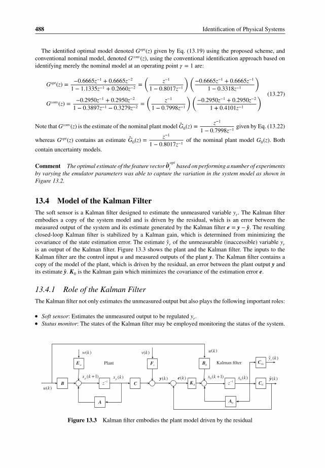
13.4 Model of the Kalman FilterThe soft sensor is a Kalman filter designed to estimate the unmeasured variable yr. The Kalman filterembodies a copy of the system model and is driven by the residual, which is an error between themeasured output of the system and its estimate generated by the Kalman filter e = y − y. The resultingclosed-loop Kalman filter is stabilized by a Kalman gain, which is determined from minimizing thecovariance of the state estimation error. The estimate yr of the unmeasurable (inaccessible) variable yr

is an output of the Kalman filter. Figure 13.3 shows the plant and the Kalman filter. The inputs to theKalman filter are the control input u and measured outputs of the plant y. The Kalman filter contains acopy of the model of the plant, which is driven by the residual, an error between the plant output y andits estimate y. K0 is the Kalman gain which minimizes the covariance of the estimation error e.

13.4.1 Role of the Kalman FilterThe Kalman filter not only estimates the unmeasured output but also plays the following important roles:

∙ Soft sensor: Estimates the unmeasured output to be regulated yr.∙ Status monitor: The states of the Kalman filter may be employed monitoring the status of the system.

1z−( 1)px k + ( )px k

( )u k

( )ky

A

B C

wE vF

( )w k ( )v k

1z−0 ( 1)x k +

0 ( )x k ˆ ( )ky

0A

0K 0C

0B

( )u k

ˆ ( )ry k

( )ke

0rCPlant Kalman filter

Figure 13.3 Kalman filter embodies the plant model driven by the residual

Soft Sensor 489

∙ Model perturbation monitor: The residual of the Kalman filer provides an estimate of the modelperturbation, which is the deviation of the plant transfer function from that of the nominal one. Thishelps in achieving the following objectives;◦ designing a robust H-infinity controller◦ ensuring superior performance of the closed-loop system over a wide range of model perturbations.

The plant is identified, and the controller redesigned whenever the residual exceeds some specifiedthreshold. Frequent identification and the design of controller using the identified model will ensuresuperior controller performance

◦ the residual may be employed for fault diagnosis.

13.4.2 Model of the Kalman Filter

x0(k + 1) = A0x0(k) + B0u(k) + K0 (y(k) − y(k))

y(k) = C0x0(k)

yr(k) = C0rx0(k)

e(k) = y(k) − y(k)

(13.28)

where(A0, B0, C0

)is the identified nominal plant model (A, B, C), x0(k) is a nx1 state, y(k) is an nyx1

estimate of the plant output y(k). Rewriting the Kalman filter model after substituting for y in thedynamical equation yields

x0(k + 1) =(A0 − K0C0

)x0(k) + B0u(k) + K0y(k)

y(k) = C0x0(k)

yr(k) = C0rx0(k)

(13.29)

13.4.3 Augmented Model of the Plant and the Kalman FilterThe augmented model

(Apk, Bpk, Cpk

)formed of the plant and the Kalman filter relating the input u(k)

and the estimate of the inaccessible output yr(k) takes the following form:

xpk(k + 1) = Apkxpk(k) + Bpku(k) + Epkw(k) + Fpkv(k)

yr(k) = Cpkxpk(k)(13.30)

where xpk(k) =[

x(k)x0(k)

], Apk =

[A 0

K0Cp A0 − K0C0

], Bpk =

[BB0

]Fpk =

[0

K0Fv

], Epk =

[Ew

0

]; Cpk =

[0 C0r

]

13.5 Robust Controller Design13.5.1 ObjectiveDesign a robust controller such that the closed-loop control system meets the stability and performancerequirements, and the output of the system, denoted y(k), tracks a given reference input r(k). In general,the output y(k) may be an element of the measured output y(k) or yr(k), which the soft sensor measures.In this chapter, the output to be regulated is chosen to be y(k) = yr(k).


rer ry0p kG0cG

v

w

u

+

+

+

+

+−

Figure 13.4 A closed-loop system formed of the augmented nominal plant and controller

13.5.2 Augmented ModelLet Gpk be the transfer function of the augmented state space model

(Apk, Bpk, Cpk

).

13.5.2.1 Nominal Augmented Model

Let Gp0k be the transfer function of the augmented nominal plant(Apk0, Bpk0, Cpk0

)formed of the nominal

plant(A0, B0, C0

r

)and the Kalman filter

(A0, B0, C0r

).

13.5.3 Closed-Loop Performance and StabilityLet Gc0 be the controller that stabilizes the nominal plant Gp0k; r(k), y(k), and er(k) are the referenceinput, the output to be regulated, and the tracking error respectively; w is the disturbance at the plantoutput; v is the measurement or sensor noise. The closed-loop formed of the augmented nominal plantand the controller is shown in Figure 13.4.

Let U and Z be respectively a 3 × 1 input vector comprising r, w, and v, and a 2 × 1 output to beregulated formed of tracking error er and control input u given by

U = [ r w v ]T (13.31)

Z = [ er u ]T (13.32)

Closed-loop transfer functions, which play significant role in the stability and performance of a controlsystem, are three sensitivity functions of the closed-loop system formed of the nominal plant and nominalcontroller [8]. They are the sensitivity S0, the (control) input sensitivity Su0, and the complementarysensitivity T0 given by:

S0 =1

1 + Gp0kGc0

Su0 = S0Gc0

T0 = 1 − S0

(13.33)

Since T0 = 1 − S0, there are essentially two sensitivity functions, namely S0 and Su0, that determine thestability and the performance. The performance objective of a control system is to regulate the trackingerror e = r − y so that the steady-state tracking error is acceptable and its transient response meets thetime and the frequency domain specifications respecting the technological constraints on the controlinput u so that, for example, the actuator is not saturated. A map relating the inputs r, w, and v and theoutputs to be regulated namely er and u are:

er = S0(r − w − v) (13.34)

u = Su0(r − v − w) (13.35)

Soft Sensor 491

The transfer matrix relating U to Z is given by

Z =

[S0 −S0 −S0

Su0 −Su0 −Su0

]U (13.36)

13.5.4 Uncertainty ModelThe numerator-denominator perturbation model, which is similar to the emulator (13.5), considers theperturbation in the numerator and denominator polynomials separately instead of clubbing together as asingle perturbation of the overall transfer function.

Gpk = NpkD−1pk =

(Np0k + ΔN

) (Dp0k + ΔD

)−1(13.37)

where Np0k and Npk are the numerator polynomials; Dp0k and Dpk are the denominator polynomialsrespectively of Gp0k and Gpk; ΔN ∈ RH∞ and ΔD ∈ RH∞ are respectively frequency dependent relativeperturbation in the numerator and the denominator polynomials [5]. The robust stability of the closed-loopsystem with plant model uncertainty is established using the small gain theorem.

Theorem 13.1 Assume that Gc0 internally stabilizes the nominal augmented plant Gp0k. Hence S0 ∈RH∞ and Su0 ∈ RH∞. Then closed-loop system is well posed and internally stable for all numerator anddenominator perturbations

‖‖‖[ΔN ΔD

]‖‖‖∞= max

𝜔

{√Δ2

N (j𝜔) + Δ2D (j𝜔)

}≤ 1∕𝛾0 (13.38)

If and only if

‖‖‖[ S0 Su0

]D−1

p0‖‖‖∞

< 𝛾0 (13.39)

Proof: The SISO robust stability problem considered herein is a special case of MIMO case proved in[14].

Thus to ensure a robustly stable closed-loop system, the nominal sensitivity S0 should be made smallin frequency regions where the denominator uncertainty ΔD is large, and the nominal complementarysensitivity Su0 should be made small in frequency regions where the numerator uncertainty ΔN is large.Our objective is to design a controller Gc0 such that robust performance and robust stability are achieved,that is, both the performance and stability hold for all plant model perturbations ‖[ΔN ΔD ]‖ ≤ 1∕𝛾0 forsome 𝛾0 > 0. Besides these requirements, we need to also consider technological constraints, especiallythe control input limitations. From Theorem 13.1 and Eq. (13.36) it is clear that the requirements forrobust stability, performance and control limitation are inter-related:

∙ Robust performance for tracking with disturbance rejection. as well as robust stability in the face ofdenominator perturbations, requires small sensitivity function S0 in the low-frequency region.

∙ Control input limitation and robust stability in the face of numerator perturbation require small controlinput sensitivity function Su0.


0cG Gp

r u

v+

−

++

y

ˆry

w

u

uW

SW

re

rwe

wu

pkG

Controller

Plant

Plant and the Kalman filter

Kalman filterWeights

Figure 13.5 Mixed sensitivity weights for closed-loop system

13.5.5 Mixed-sensitivity Optimization ProblemWith a view to address these requirements, let us select regulated outputs to be a frequency weightedtracking error erw, and a weighted control input uw to meet respectively the requirements of performanceand control input limitation.

Zw = [ erw uw ]T (13.40)

where Zw is 2 × 1 vector output to be regulated, ew and uw are defined by their respective Fouriertransforms: erw(j𝜔) = er(j𝜔)WS(j𝜔) and uw(j𝜔) = u(j𝜔)Wu(j𝜔). Figure 13.5 shows the weighted trackingerror and the control input for the closed-loop system formed of the augmented plant Gpk comprisingthe plant and the Kalman filter. The frequency weights are chosen such that their inverses are the upperbound on the respective sensitive functions so that weighted sensitive functions are less than unity.The weighting functions WS(j𝜔) and Wu(j𝜔) provide the tools to specify the tradeoff between robustperformance and robust stability for a given application. For example, if robust performance (and robuststability to denominator perturbation ΔD) is more important than the control input limitation, then theweighting function WS is chosen to be large compared to Wu. To emphasize control limitation (and robuststability to numerator perturbation ΔN) the weighting function Wu is chosen to be large compared to WS.For steady-state tracking with disturbance rejection in the weighting function WS one may include anapproximate but “stable integrator” by choosing a pole close to zero or close to unity for the continuous-time and the discrete-time cases respectively [14]. Let Trz be the nominal transfer matrix (when the plantperturbation Δ0 = 0) relating the reference input to the two frequency weighted outputs zw, which isfunction of the Gp0k and Gc0 given by

Trz

(Gc0, Gp0k

)= D−1

p0k

[WSS0 WuSu0

]T(13.41)

where Ws = Dp0kWs and Wu = Dp0kWu so that the D−1p0k term appearing in the mixed sensitivity measure

Trz is canceled, thus yielding the following simplified measure Trz =[

WSS0 WuSu0

]T. The mixed-

sensitivity optimization problem for robust performance and stability in the H∞ framework is thenreduced to finding the controller Gc0 such that:

‖‖‖Trz

(Gc0, Gp0k

)‖‖‖∞= ‖‖‖[ WSS0 WuSu0

]‖‖‖∞= max

𝜔

{√(WSS0 (j𝜔)

)2 +(WuSu0 (j𝜔)

)2}

≤ 𝛾 < 1

(13.42)

Soft Sensor 493

It is shown in [14] that the robustness condition (13.42) guarantees not only robust stability but alsorobust performance all ‖[ΔN ΔD ]‖∞ ≤ 1∕𝛾: that is for all perturbations constrained by the inequality(13.38).

13.5.6 State-Space Model of the Robust Control SystemLet the state-space model of the H-infinity robust controller Gc0 be

xc(k + 1) = Acxc(k) + Bcer(k)

u(k) = Ccxc(k) + Dcer(k)(13.43)

where er(k) = r(k) − yr(k) is the tracking error. Substituting for yr(k), the expression for the control inputu(k) becomes

u(k) = Ccxc(k) − DcC0rx0(k) + Dcr(k) (13.44)

The closed-loop control system formed of the augmented plant(Apk, Bpk, Cpk

)given by Eq. (13.30) and

the controller Eqs. (13.43) and (13.44) becomes

x(k + 1) = Ax(k) + Br(k) + Ew(k) + Fv(k)

yr(k) = C0rx(k)(13.45)

where A =⎡⎢⎢⎣

Ap −B0DcC0r BpCc

K0Cp A0 − K0C0 − B0DcC0r B0Cc

0 −BcC0r Ac

⎤⎥⎥⎦ ; B =⎡⎢⎢⎣

BpDc

B0Dc

Bc

⎤⎥⎥⎦E =

⎡⎢⎢⎣0

K0Fp

0

⎤⎥⎥⎦ , F =⎡⎢⎢⎣

Fpk

00

⎤⎥⎥⎦ ; C =[

0 C0r 0]

Figure 13.6 shows the closed-loop control system using a soft sensor. The unmeasured output of theplant yr is substituted by its estimate yr computed using the soft sensor (Kalman filter). The closed-loopsystem (13.45) is robustly stable as long as the perturbations of the nominal plant and the Kalman filtersatisfy the robust stability condition (13.42) when perturbations in the numerator and the denominatorpolynomials of the augmented plant defined by Eq. (13.37) satisfy the inequality (13.38). The pertur-bation ΔN in the numerator polynomial Npk and perturbation ΔD in the denominator polynomial Dpk

0 ( )cG z ( )zGr

u

Controller

Plant

Kalman filter

Plant

model

υ+

−

++

y

0K

ˆry

e

y

w

Figure 13.6 Closed-loop control with soft sensor


of the augmented nominal plant Gp0k result from the perturbations in the nominal state-space model(Ap0k, Bp0k, Cp0k

).

13.6 High Performance and Fault Tolerant Control SystemThe Kalman filter residual is employed for achieving the additional tasks of high performance controlsystem, performance monitoring, and fault diagnosis. The plant transfer function G(z) relating the controlinput u(z) and the regulated output y(z) is:

G(z) = N(z)D(z)

(13.46)

The plant output y(z) is given by

y(z) = G(z)u(z) + 𝜐(z) (13.47)

13.6.1 Residual and Model-mismatchAn expression relating the residual and the model perturbation takes the following form:

In [4], the relation between the residual e = y − y and the Kalman filter inputs u and y is shown to be

e(z) =D0(z)

F0(z)y(z) −

N0(z)

F0(z)u(z) (13.48)

where F0(z) = det(zI − A0 + K0C0)

), N0(z), D0(z) and G0(z) are the nominal numerator, nominal denom-

inator, and nominal transfer functions respectively of N(z), D(z), and G(z) given by Eq. (13.46). Further,an expression for the residual e of the Kalman filter for the closed-loop system formed of the plant, theKalman filter, and the robust controller (13.45) is derived using the relation between the residual andmodel-mismatch for an open-loop system formed of the plant and the Kalman filter given in [4] and theexpression (13.48). Expression for the residual is given by

e(z) = ef (z) + e0(z) (13.49)

ef (z) = Su0(z)ΔGrfilt(z) (13.50)

e0(z) = 𝜐filt(z) (13.51)

where the model-mismatch term ΔG = G − G0. Expressing plant model-mismatch ΔG in terms ofperturbation in the numerator and the denominator polynomials of the plant transfer function similar toEq. (13.37) (where the perturbation covers both plant and the Kalman filter models), we get

G = ND−1 =(N0 + ΔN

) (D0 + ΔD

)−1(13.52)

rfilt(z) and 𝜐filt(z) are the filtered reference input r and filtered noise respectively:

rfilt =D0(z)

F0(z)r(z)

𝜐filt =D0(z)

F0(z)𝜐(z)

(13.53)

Soft Sensor 495

The residual expression (13.49) forms the basis for developing a high performance and fault tolerantcontrol system. The model mismatch will be nonzero if the actual plant model deviates from the nominalmodel. The mean of the residual is an indicator of a model mismatch. We will assume that e0(k) continuesto be a zero-mean Gaussian white noise process under both fault and fault-free conditions. It is shownin [4]

E [e] = 0 if and only if ΔGp(z) ≡ 0 (13.54)

13.6.2 Bayes Decision StrategyWe will formulate a binary hypothesis testing problem to decide between two hypotheses, H0 and H1,where H0 denotes a normal (or an acceptable) operating regime and H1 indicates an abnormal (or anunacceptable) operating regime. A batch processing scheme is adopted here where residuals are collectedin a sliding time window of length N and processed at each time instant. At each time instant k, the Nresiduals formed of the present and past N − 1 residuals, e(k − i) : i = 0, 1, 2,…N − 1, are collected:

e(k) =[

e(k) e(k − 1) e(k − 2) . e(k − N + 1)]T

(13.55)

The Bayes decision strategy takes the general form

ts(e)

{≤ 𝜂 normal> 𝜂 abnormal

(13.56)

where ts(e) is the test statistics of the residual e and 𝜂 is the threshold value computed taking into accountthe variance of the noise term e0(k), prior probabilities of the two hypotheses, the cost associated withcorrect and wrong decisions, and the probability of false alarm. Test statistics for a reference input r(k)that is either a constant or a sinusoid of frequency f0 or an arbitrary signal are all listed below [15]:

ts(e) =

⎧⎪⎪⎪⎨⎪⎪⎪⎩

|||||| 1N

k∑i=k−N+1

e(i)|||||| r(k) = constant

Pee(f0) r(k) is a sinusoid

1N

k∑i=k−N+1

e2(i) r(k) is an arbitrary signal

(13.57)

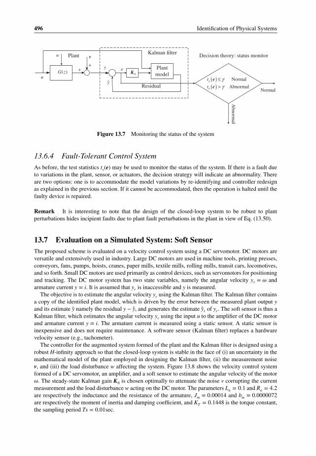
13.6.3 High Performance Control SystemThe performance of the robust controller depends upon (i) the accuracy of the estimate yr of the outputto be regulated yr and is generated by the Kalman filter-based soft sensor, (ii) noise and the disturbanceaffecting the output, and (iii) the plant model deviation ΔG. In order to meet the requirement of highperformance and stability in the design stage, the control input sensitivity function Su0(z) is given anappropriate frequency weight Wu(z) in the mixed sensitivity H-infinity design setting so that resultingcontroller will ensure that the residual is small in the face of plant deviation, as can be inferred fromEq. (13.50). When Su0(z) is small, then the residual will be small and hence the true and the estimatedvariable are close ensuring thereby acceptable controller performance. In the operational stage, the teststatistics ts(e) is monitored using Eq. (13.56) as shown in Figure 13.7. When an abnormal operatingregime is indicated, then the plant is re-identified and the robust controller is redesigned for the identifiedplant model. It is an indirect adaptive control scheme. The Kalman gain K0 is chosen optimally to ensurethat covariance of the estimation error is minimum.


PlantKalman filter

Plant

model

Residual

Decision theory: status monitor

( )( )

Normal

NormalAbnormal

Ab

no

rmal

s

s

t

t

γγ

≤>

e

e

( )G zu

v

++ y

0Ke

y

w

Figure 13.7 Monitoring the status of the system

13.6.4 Fault-Tolerant Control SystemAs before, the test statistics ts(e) may be used to monitor the status of the system. If there is a fault dueto variations in the plant, sensor, or actuators, the decision strategy will indicate an abnormality. Thereare two options: one is to accommodate the model variations by re-identifying and controller redesignas explained in the previous section. If it cannot be accommodated, then the operation is halted until thefaulty device is repaired.

Remark It is interesting to note that the design of the closed-loop system to be robust to plantperturbations hides incipient faults due to plant fault perturbations in the plant in view of Eq. (13.50).

13.7 Evaluation on a Simulated System: Soft SensorThe proposed scheme is evaluated on a velocity control system using a DC servomotor. DC motors areversatile and extensively used in industry. Large DC motors are used in machine tools, printing presses,conveyors, fans, pumps, hoists, cranes, paper mills, textile mills, rolling mills, transit cars, locomotives,and so forth. Small DC motors are used primarily as control devices, such as servomotors for positioningand tracking. The DC motor system has two state variables, namely the angular velocity yr = 𝜔 andarmature current y = i. It is assumed that yr is inaccessible and y is measured.

The objective is to estimate the angular velocity yr using the Kalman filter. The Kalman filter containsa copy of the identified plant model, which is driven by the error between the measured plant output yand its estimate y namely the residual y − y, and generates the estimate yr of yr. The soft sensor is thus aKalman filter, which estimates the angular velocity yr using the input u to the amplifier of the DC motorand armature current y = i. The armature current is measured using a static sensor. A static sensor isinexpensive and does not require maintenance. A software sensor (Kalman filter) replaces a hardwarevelocity sensor (e.g., tachometer).

The controller for the augmented system formed of the plant and the Kalman filter is designed using arobust H-infinity approach so that the closed-loop system is stable in the face of (i) an uncertainty in themathematical model of the plant employed in designing the Kalman filter, (ii) the measurement noisev, and (iii) the load disturbance w affecting the system. Figure 13.8 shows the velocity control systemformed of a DC servomotor, an amplifier, and a soft sensor to estimate the angular velocity of the motor𝜔. The steady-state Kalman gain K0 is chosen optimally to attenuate the noise v corrupting the currentmeasurement and the load disturbance w acting on the DC motor. The parameters La = 0.1 and Ra = 4.2are respectively the inductance and the resistance of the armature, Jm = 0.00014 and bm = 0.0000072are respectively the moment of inertia and damping coefficient, and KT = 0.1448 is the torque constant,the sampling period Ts = 0.01sec.

Soft Sensor 497

1

a asL R+1

m mJ s b+

TK

TKAKu

ω

i

w

0Kie

i

ωi

u

v

0ωcG

Plant: DC motor: Gp

Controller

Kalman filter

Model of

the plant

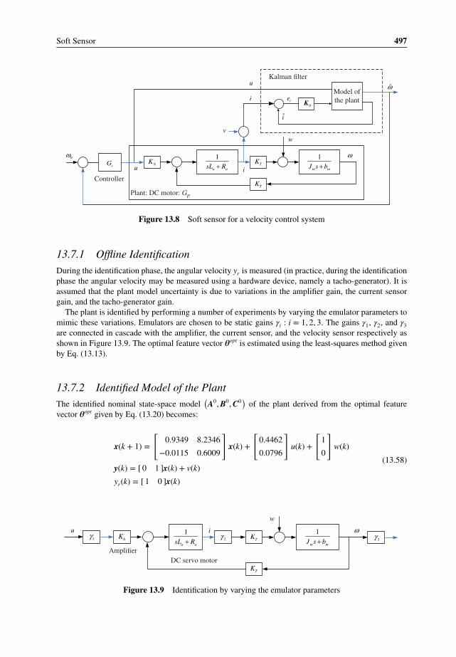
Figure 13.8 Soft sensor for a velocity control system

13.7.1 Offline IdentificationDuring the identification phase, the angular velocity yr is measured (in practice, during the identificationphase the angular velocity may be measured using a hardware device, namely a tacho-generator). It isassumed that the plant model uncertainty is due to variations in the amplifier gain, the current sensorgain, and the tacho-generator gain.

The plant is identified by performing a number of experiments by varying the emulator parameters tomimic these variations. Emulators are chosen to be static gains 𝛾i : i = 1, 2, 3. The gains 𝛾1, 𝛾2, and 𝛾3

are connected in cascade with the amplifier, the current sensor, and the velocity sensor respectively asshown in Figure 13.9. The optimal feature vector 𝜽opt is estimated using the least-squares method givenby Eq. (13.13).

13.7.2 Identified Model of the PlantThe identified nominal state-space model

(A0, B0, C0) of the plant derived from the optimal feature

vector 𝜽opt given by Eq. (13.20) becomes:

x(k + 1) =

[0.9349 8.2346

−0.0115 0.6009

]x(k) +

[0.4462

0.0796

]u(k) +

[1

0

]w(k)

y(k) = [ 0 1 ]x(k) + v(k)

yr(k) = [ 1 0 ]x(k)

(13.58)

1

a asL R+1

m mJ s b+TK

TK

AKu ωi

w

1γ 2γ 3γ

Amplifier

DC servo motor

Figure 13.9 Identification by varying the emulator parameters


The state-space model of the Kalman filter given by Eq. (13.29) is

x0(k + 1) =

[0.9349 8.2209

−0.0115 0.5998

]x0(k) +

[0.4462

0.0796

]u(k) +

[0.0137

0.0011

]y(k)

yr(k) = [ 1 0 ]x0(k)

(13.59)

The Kalman gain K0 =[

0.01370.0011

]is computed for the covariance of the disturbance Q0 = 0.1 and the

measurement noise variance R0 = 100.

Comments The uncertainty model used in the physical system is different from that used in the case ofthe simulated velocity control system. In this case, the emulator was chosen to target only those modelparameters that are likely to vary, while in the case of the simulated example an unstructured emulatormodel was employed. However, the design of the robust controller was similar to that of the simulatedexample.

Recall that the Kalman filter computes the estimate by fusing the a posteriori information provided bythe measurement, and the a priori information contained in the model that generated the measurement.The covariance of the measurement noise and the covariance of the disturbance quantify the degree ofbelief associated with the measurement and model information, respectively. These covariances play acrucial role in the performance of the Kalman filter. The estimate of the state is obtained as the bestcompromise between the estimates generated by the model and those obtained from the measurement,depending upon the plant noise and the measurement noise covariances.

As the covariance of the disturbance Q0 = 0.1 is very small compared to that of the measurementnoise variance R0 = 100, that is Q∕R is very small, the Kalman filter model (A0, B0, C0) is assumed tobe more accurate compared to the measurement y. This is reflected in the “size” of the Kalman gainK0 which is “small.” As a result, the Kalman filter computes the estimate by giving more weight to themodel than the noisy measurement.

13.7.3 Mixed-Sensitivity Optimization ProblemFrequency weights WS(z) associated with the sensitivity functions S0(z) and Wu(z) associated withcontrol input sensitivity Su0(z) were determined using a recursive design procedure, to obtain an accept-able tradeoff between the steady-state tracking requirement and control input limitation in the mixed

sensitivity problem (13.42). The frequency weights were Ws(z) = 0.11 − 0.99z−1

emphasizing very low

frequency for tracking a constant reference input and Wu(z) = 0.1. The H∞ robust controller given byEq. (13.43) is:

xc(k + 1) =

⎡⎢⎢⎢⎢⎢⎢⎣

0.99 0 0 0 0

0 0.7674 1 0 0

0 −0.0667 0.7674 0.3354 0.205

0 0 0 0.7679 1

3.077 0.0363 −0.0417 −0.4734 −0.5267

⎤⎥⎥⎥⎥⎥⎥⎦xc(k) +

⎡⎢⎢⎢⎢⎢⎢⎣

0.0395

0

0

0

0.0611

⎤⎥⎥⎥⎥⎥⎥⎦er(k)

u(k) =[

6.9928 0.0824 −0.0947 −0.9235 −2.8421]

xc(k) + 0.1389er(k)

(13.60)

As the controller has a pole at 0.99(which is close to the origin of the z-plane), a steady-state tracking ofa constant reference input is ensured.

Soft Sensor 499

0 0.5 10

1

2A: Velocity and its estimate

Ste

p

0 0.5 1-0.05

0

0.05B: Current and its estimate

0 0.5 10

2

4C: Velocity and its estimate

Ste

p

0 0.5 1-0.1

0

0.1D: Current and its estimate

0 0.5 10

1

2E: Velocity and its estimate

Ste

p

0 0.5 1-0.05

0

0.05F: Current and its estimate

0 0.5 10

1

2G: Velocity and its estimate

Ste

p

0 0.5 1-0.05

0

0.05H: Current and its estimate

Figure 13.10 Velocity and current profiles and their estimates for different operating regimes

13.7.4 Performance and RobustnessVarious operating regimes were simulated including:

∙ Nominal operating regime: The plant state model is equal to the nominal model (Ap0, Bp0, Cp0).∙ Plant perturbations: The plant state-space model (Ap, Bp, Cp) is subject to perturbations:

◦ Ap = Ap0(1 + ΔA)◦ Bp = Bp0(1 + ΔB)◦ Cp = Cp0(1 + ΔC)where ΔA = 0.2, ΔB = 0.2, and ΔC = 0.2 The results of normal and perturbed parameter experimentsare shown in Figure 13.10. The current, the velocity, and their estimates from the Kalman filterare displayed under different operating regimes. The estimated velocity and the current generatedby the Kalman filter and those from the plant are shown. Subfigures (a) and (b) show respectivelythe velocity and the current profiles under the normal operating regime. Similarly, subfigures (c)and (d), subfigures (e) and (f), and subfigures (g) and (h) show the plots of the estimated velocityand the estimated current respectively under perturbations Ap = Ap0(1 + ΔA), Bp = Bp0(1 + ΔB), andCp = Cp0(1 + ΔC). The tracking performance of the velocity control system using the estimatedregulated variable yr in the face of plant perturbations is very good. The steady-state tracking error isnegligible and transient performance is good. Further, the Kalman filter estimate meets requirementsof (i) accuracy and (i) low estimation error variance. Note that estimates of both current and velocityestimates are practically noise-free even though Kalman filter inputs, namely the current and controlinput, are both noisy.

13.7.5 Status MonitoringThe status of the system is monitored in the face of the plant perturbation, and in the presence of thenoise and disturbances corrupting the plant output. The residual, which is an error between the current


0 0.5

-0.05

0

0.05

A: Nominal

Resid

ual

-0.5 0 0.5

-0.02

0

0.02

0.04

0.06

0.08

B: Nominal

Corr

ela

tion

Lag

0 0.5

-0.05

0

0.05

C: Del A

Time

-0.5 0 0.5

-0.02

0

0.02

0.04

0.06

0.08

D: Del A

Lag

0 0.5

-0.05

0

0.05

E: Del B

-0.5 0 0.5

-0.02

0

0.02

0.04

0.06

0.08

F: Del B

Lag

0 0.5

-0.05

0

0.05

G: Del C

Time

-0.5 0 0.5

-0.02

0

0.02

0.04

0.06

0.08

H: Del C

Lag

Figure 13.11 Residuals and their auto-correlations under plant perturbations

and its estimate using the Kalman filter, and the auto-correlations of the residual were also computed, asshown in Figure 13.11.

Subfigures (a) and (b) show respectively the residual and its auto-correlation under the normal operatingregime. Similarly, subfigures (c) and (d), (e) and (f), and (g) and (h) show respectively the plots of theresidual and its auto-correlation under perturbations Ap = Ap0(1 + ΔA), Bp = Bp0(1 + ΔB) and Cp =Cp0(1 + ΔC). The mean of residual is nonzero under plant perturbations. The auto-correlation function ofthe residual visually enables us to distinguish the normal from abnormal operating conditions resultingfrom plant perturbations. The test statistics ts(e) under various plant perturbations are given in Table13.1. It is important to emphasize that the performance of the Kalman filter operating in an open-loopconfiguration (when the Kalman filter estimate is not employed to drive the controller to close the loop)is poor in the face of plant perturbations. In other words, the performance of the Kalman filter is superiorwhen operating in a closed-loop with its estimate driving the controller, as shown in Figure 13.8.

13.8 Evaluation on a Physical Velocity Control SystemMATLAB® Real time workshop is used to implement and evaluate the performance of the pro-posed soft sensor in a real-time environment on a laboratory-scale physical velocity control system.

Table 13.1 The test statistics

Normal Ap = Ap0(1 + ΔA) Bp = Bp0(1 + ΔB) Cp = Cp0(1 + ΔC)

0.0074 0.0244 0.0106 0.0235

Soft Sensor 501

1

a asL R+1

m mJ s b+TK

TK

AKu

ControllerAmplifier

DC servo motor

D/A

A/D

Kalman filter

ω

i

w

ω

r

i

Figure 13.12 Physical DC motor with amplifier is interfaced to the real-time workshop

The physical velocity control system is similar to that of the simulated system given in the Sec-tion 13.7. A host PC is employed to design the controller using MATLAB®. The target PC is inter-faced to an A/D to acquire the current from the DC motor, and the estimated angular velocity fedto the D/A converter I/O board, termed Data Translation DT 2821. The host PC downloads the exe-cutable code of the Simulink model in C++ to the target PC. The target PC executes the code inreal time using the sampled input from A/D converter, and the soft sensor output is fed to the D/Aconverter. Figure 13.12 shows the laboratory-scale physical position control system interfaced to apersonal computer using analog to digital and digital to analog converters, and its block diagramrepresentation.

In order to identify the plant and to evaluate the performance, the tachometer was connected tothe DC motor to measure the velocity merely for comparing the estimated velocity from the Kalmanfilter with the actual velocity. The plant was identified by performing a number of parameter-perturbedexperiments. The static gain emulators were connected in cascade with the amplifier, the current sensor,and the velocity sensors, as shown in Figure 13.9.

Figure 13.13 shows the actual and the estimated current and the angular velocity. The figure on theleft shows the velocity while that on the right shows the current profiles.

It can be deduced that the estimate of current and the angular velocity given by the Kalman filterclosely matches that sensed by the current sensor and the tachometer respectively. The noise spikes inthe current and the velocity are due to the commutator and the brush associated with the armature of theDC motor.


-400

-300

-200

-100

0

100

Velo

city

Velocity from System and Observer at Observer Pole = (0,0)

0 0.5 1 1.5 2 2.5 3 3.5 4 4.5 5-1.5

-1

-0.5

0

0.5

1

1.5

2

Time (sec)

0 0.5 1 1.5 2 2.5 3 3.5 4 4.5 5

Time (sec)

Cu

rre

nt

Current from System and Observer at Observer Pole = (0,0)

Figure 13.13 Velocity, current, and their estimates

Comments The identified model of the plant using the proposed parameter perturbed identificationscheme was robust in the face of model uncertainties associated with friction, nonlinearity, and variationsin the operating points.

The performance of the Kalman filter, whose design is based on the nominal identified model andthe estimates of noise and the disturbance variances, in estimating the angular velocity of the physicalsystem is very promising.

The closed action of the closed-loop velocity control system, as well as the Kalman filter drivenrespectively by the tracking error and the residual, thanks to the design and implementation of the robustcontroller, contributed to the superior performance of the fault tolerant velocity control system. Theeffect of the disturbance on the output is attenuated and the sensitivity to model mismatch is reduced.

13.9 ConclusionsThe reliable identification scheme of the plant using a number of parameter-perturbed experiments byemulating likely fault scenarios is key to ensure high performance and robust stability in the face ofmodel uncertainty and variation in the operating conditions

The robust controller based on minimizing frequency-weighted combinations of sensitivity and controlinput sensitivity functions in the mixed sensitivity H-infinity setting is effective in meeting the require-ments of accuracy of the Kalman filter estimate, the performance and stability in the face of plant modelperturbations. The tracking performance of the control system using the estimated regulated variablein the face of plant perturbations is highly promising. The steady-state tracking error is negligible andtransient performance is good.

The Kalman filter residual is very effective in monitoring the status of the system. The auto-correlationfunction of the residual visually enables us to distinguish the normal from abnormal operating conditionsresulting from plant perturbations.

The residual is employed in both the design and in operational stages. In the operational stage,whenever the test statistics indicate an abnormal operating regime, the plant is identified and the controlleris redesigned to achieve a high performance control system. If the controller cannot accommodate tomodel the perturbations, a fault is indicated, and the system is shut down for repair.

The performance of a fault tolerant control system is highly promising in the face of noise and distur-bance, model uncertainty, and variation in the operating conditions thanks to the reliable identification ofthe plant and the robust controller design. The Kalman filter plays a key role in providing a maintenance-free soft sensor to estimate unmeasured or inaccessible variables, and in monitoring the status of thesystem.

The proposed scheme was evaluated on simulated and physical laboratory-scale velocity controlsystems.

Soft Sensor 503

13.10 Summary

Mathematical FormulationThe state-space model of a system is given by:

x(k + 1) = Ax(k) + Bu(k) + Eww(k)

y(k) = Cx(k) + Fvv(k)

yr(k) = Crx(k)

Transfer Function Model

y(z) = N(z)D(z)

u(z) +Nw(z)

D(z)w(z) + Fvv(z)

Rewriting by cross-multiplying by D(z),we get:

D(z)y(z) = N(z)u(z) + 𝝊(z)

where 𝝊(z) = Nw(z)w(z) + D(z)Fvv(z)The ny × 1 matrix transfer function G(z) of the system is given by:

G(z) = N(z)D−1(z)

Emulator: Numerator-denominator Perturbation Model

G(z) = N(z)D(z)

=(I + ΔN(z)

)(1 + ΔD(z)

) N0(z)

D0(z)= Ge(z)G0(z)

where G0(z), is the nominal transfer function, N0(z) is the nominal the numerator (matrix) polynomial,

D0(z) is the nominal denominator (scalar) polynomial; Ge(z) =(

I + ΔN(z)

1 + ΔD(z)

)is the nyxny emulator;

ΔN(z) ∈ RH∞ and ΔD(z) ∈ RH∞

Selection of the Emulator Model

Ge(z) =

⎡⎢⎢⎢⎢⎣Ge1(z) 0 0 0

0 Ge2(z) 0 0

. 0 . .

0 0 0 Geny(z)

⎤⎥⎥⎥⎥⎦

Gei(z) =

⎛⎜⎜⎜⎜⎜⎜⎜⎜⎝

𝛾i gain

𝛾iz−d gain and pure delay

𝛾i

𝛾i1 + z−1

1 + 𝛾i1z−1first order all pass

𝛾i

∏j

𝛾ij + z−1

1 + 𝛾ijz−1Blaschke product

The parameters 𝛾i and 𝛾ij are termed herein emulator parameters.


Identification of the System: Reliable SchemeThe perturbed model at the jth experiment relating the input u(z) and the ith output yj

i(z) is:

Dj(z)yji(z) = Nj

i (z)u(z) + 𝜐ji(z)

The linear regression model becomes:

yii(k) =

(𝝍 i

i(k))T𝜽j

i + 𝝊ji(k) i = 1, 2, 3,… , ny

where(𝝍

ji(k)

)T=

[−yj

i(k − 1) −yji(k − 2) . −yj

i(k − n) u(k − 1) . u(k − n)]𝜽j

i is a Mx1 vectorof unknown model parameter given by:

𝜽ji =

[aj

1 aj2 . aj

n bji1 bj

i2 . bjin

]T

Least-Squares Estimation

��opt

i = arg

{min{𝜃i}

{Nexp∑j=1

N∑k=1

(yj

i(k) −(𝝍 j

i

)T

(k)𝜽i

)T(yj

i(k) −(𝝍 j

i

)T

(k)𝜽i

)}}

yj opti (k) =

(𝝍 j

i

)T(k)��

opt

i

Identified Nominal ModelThe “optimal nominal model” derived from the optimal estimate ��

opt

i becomes:

Dopt(z)y(z) = Nopt(z)u(z) + 𝝊(z)

where Dopt(z) and Nopt(z) are derived from ��0

i :i = 1, 2,… , ny. The optimal nominal model is:

Gopt(z) = Nopt(z)Dopt(z)

The identified nominal state-space model, denoted(A0, B0, C0

)of (A, B, C) is:

x(k + 1) = A0x(k) + B0u(k)

y(k) = C0x(k)

yr(k) = Cr0x(k)

The Nominal Plant ModelLet the nominal plant model

(A0, B0, C0) be:

x(k + 1) = A0x(k) + B0u(k) + Eww(k)

y(k) = C0x(k) + Fvv(k)

yr(k) = C0r x(k)

Soft Sensor 505

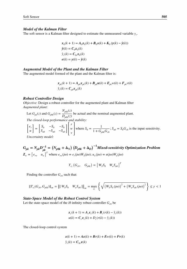
Model of the Kalman FilterThe soft sensor is a Kalman filter designed to estimate the unmeasured variable yr.

x0(k + 1) = A0x0(k) + B0u(k) + K0 (y(k) − y(k))

y(k) = C0x0(k)

yr(k) = C0rx0(k)

e(k) = y(k) − y(k)

Augmented Model of the Plant and the Kalman FilterThe augmented model formed of the plant and the Kalman filter is:

xpk(k + 1) = Apkxpk(k) + Bpku(k) + Epkw(k) + Fpkv(k)

yr(k) = Cpkxpk(k)

Robust Controller DesignObjective: Design a robust controller for the augmented plant and Kalman filterAugmented plant:

Let Gpk(z) and Gp0k(z) =Np0k(z)

Dp0k(z)be actual and the nominal augmented plant.

The closed-loop performance and stability:[er

u

]=

[S0 −S0 −S0

Su0 −Su0 −Su0

] ⎡⎢⎢⎣rwv

⎤⎥⎥⎦ where S0 = 11 + Gp0kGc0

; Su0 = S0Gc0 is the input sensitivity.

Uncertainty model:

Gpk = NpkD−1pk

=(Np0k + 𝚫N

) (Dp0k + 𝚫D

)−1Mixed-sensitivity Optimization Problem

Zw =[

erw uw

]Twhere erw(j𝜔) = er(j𝜔)WS(j𝜔); uw(j𝜔) = u(j𝜔)Wu(j𝜔)

Trz

(Gc0, Gp0k

)=

[WSS0 WuSu0

]T

Finding the controller Gc0 such that:

‖Trz(Gc0, Gp0k)‖∞ = ‖‖[ WSS0 WuSu0 ]‖‖∞ = max𝜔

{√(WSS0 (j𝜔)

)2 +(WuSu0 (j𝜔)

)2}

≤ 𝛾 < 1

State-Space Model of the Robust Control SystemLet the state-space model of the H-infinity robust controller Gc0 be

xc(k + 1) = Acxc(k) + Bc(r(k) − yr(k))

u(k) = Ccxc(k) + Dc(r(k) − yr(k))

The closed-loop control system

x(k + 1) = Ax(k) + Br(k) + Ew(k) + Fv(k)

yr(k) = C0rx(k)


where A =⎡⎢⎢⎣

Ap −B0DcC0r BpCc

K0Cp A0 − K0C0 − B0DcC0r B0Cc

0 −BcC0r Ac

⎤⎥⎥⎦ ; B =⎡⎢⎢⎣

BpDc

B0Dc

Bc

⎤⎥⎥⎦E =

⎡⎢⎢⎢⎣0

K0Fp

0

⎤⎥⎥⎥⎦ , F =⎡⎢⎢⎢⎣

Fpk

0

0

⎤⎥⎥⎥⎦ ; C =[

0 C0r 0]

High Performance and Fault Tolerant Control System

y(z) = G(z)u(z) + 𝜐(z) where F0(z) = det(zI − A0 + K0C0)

).

The expression for the residual e is given by

e(z) = ef (z) + e0(z)

ef (z) = Su0(z)ΔGprfilt(z)

e0(z) = 𝜐filt(z)

where the model mismatch term ΔG = G − G0.

G = ND−1 == (N0 + ΔN)(D0 + ΔD)−1

rfilt(z) and 𝜐filt(z) are the filtered reference input r and filtered noise respectively:

rfilt =D0(z)

F0(z)r(z); 𝜐filt =

D0(z)

F0(z)𝜐(z)

E [e] = 0 if and only if ΔGp(z) ≡ 0

Bayes Decision StrategyThe Bayes decision strategy takes the general form

ts(e)

{≤ 𝜂 normal> 𝜂 abnormal

where e(k) =[

e(k) e(k − 1) e(k − 2) . e(k − N + 1)]T

, ts(e) is the test statistics of the residual eand 𝜂 is the threshold value

ts(e) =

⎧⎪⎪⎪⎨⎪⎪⎪⎩

|||||| 1N

k∑i=k−N+1

e(i)|||||| r(k) = cons tan t

Pee(f0) r(k) is a sin usoid

1N

k∑i=k−N+1

e2(i) r(k) is an arbitrary signal

Soft Sensor 507

References

[1] Kadlec, P., Gabrys, B., and Strandt, S. (2009) Data driven soft sensors in the process industry. Computers andChemical Engineering, 33, 795–814.

[2] Fortuna, L., Graziani, S., and Xibilia, G. (2007) Soft Sensors for Monitoring and Control of Industrial Processes.Springer-Verlag.

[3] Angelov, P. and Kordon, A. (2010) Adaptive inferential sensors based on evolving fuzzy models. IEEE Trans-actions on Systems, Man and Cybernetics: Case Study, 40(2), 529–539.

[4] Doraiswami, R. and Cheded, L. (2013) A unified approach to detection and isolation of parametric faults usinga Kalman filter residuals. Journal of Franklin Institute, 350(5), 938–965.

[5] Doraiswami, R. and Cheded, L. (2013) Fault diagnosis of a sensor network: a distributed filtering approach.Journal of Dynamic Systems, Measurement and Control, 135(5), 1–10.

[6] Doraiswami, R. and Cheded, L. (2012) Kalman filter for fault detection: an internal model approach. IET ControlTheory and Applications, 6(5), 1–11.

[7] Doraiswami, R., Diduch, C., and Tang, J. (2010) A new diagnostic model for identifying parametric faults.IEEE Transactions on Control System Technology, 18(3), 533–544.

[8] Goodwin, G.C., Graeb, S.F, and Salgado, M.E. (2001) Control System Design. Prentice Hall, New Jersey.[9] Kwakernaak, H. (1993) Robust control and H-inf optimization: tutorial paper. Automatica, 29(2), 255–273.

[10] Cerone, V., Milanese, M. and Regruto, D. (2009) Yaw stability control design through mixed sensitivityapproach. IEEE Transactions on Control Systems Technology, 17(5), 1096–1104.

[11] Tan, W., Marquez, H.J., Chen, T., and Gooden, R. (2001) H infinity Control Design for Industrial Boiler,Proceedings of The American Control Conference, Virginia, USA.

[12] Doraiswami, R. and Cheded, L. (2012) Robust fault tolerant controller. IECON 2012 IEEE Industrial ElectronicsSociety, Montreal.

[13] Yao, B. and Palmer, A. (2002) Indirect adaptive robust control of SISO nonlinear systems in semi-strict forms.15th IFAC World Congress, Barcelona, Spain.

[14] Zhou, K., Doyle, J., and Glover, K. (1996) Robust Optimal Control. Prentice Hall, New Jersey.[15] Kay, S.M. (1993) Fundamentals of Signal Processing: Estimation Theory. Prentice Hall PTR, New Jersey.

Identification of Physical Systems (Applications to Condition Monitoring, Fault Diagnosis, Soft...

Documents

Transcript of Identification of Physical Systems (Applications to Condition Monitoring, Fault Diagnosis, Soft...