Identification and estimation of panel data models with...
129
Identification and Estimation of Panel Data Models with Attrition Using Refreshment Samples submitted in partial fulfilment of the requirements for the degree of Doctor of Philosophy (PhD) University College London (UCL) Pierre Hoonhout January 2011
Transcript of Identification and estimation of panel data models with...

Identification and Estimation
of Panel Data Models with Attrition
Using Refreshment Samples
submitted in partial fulfilment of the requirements
for the degree of Doctor of Philosophy (PhD)
University College London (UCL)
Pierre Hoonhout
January 2011

Declaration
I, Pierre Hoonhout, confirm that the work presented in this thesis is my own.
Where information has been derived from other sources, I confirm that this
has been indicated in the thesis.
Pierre Hoonhout
2

Abstract
This thesis deals with attrition in panel data. The problem associated with at-
trition is that it can lead to estimation results that suffer from selection bias.
This can be avoided by using attrition models that are sufficiently unrestric-
tive to allow for a wide range of potential selection. In chapter 2, I propose
the Sequential Additively Nonignorable (SAN) attrition model. This model
combines an Additive Nonignorability assumption with the Sequential At-
trition assumption, to just-identify the joint population distribution in Panel
data with any number of waves. The identification requires the availability of
refreshment samples. Just-identification means that the SAN model has no
testable implications. In other words, less restrictive identified models do not
exist.
To estimate SAN models, I propose a weighted Generalized Method of Mo-
ments estimator, and derive its repeated sampling behaviour in large sam-
ples. This estimator is applied to the Dutch Transportation Panel and the
English Longitudinal Study of Ageing. In chapter 4, a likelihood-based al-
ternative estimation approach is proposed, by means of an EM algorithm.
Maximum Likelihood estimates can be useful if it is hard to obtain an explicit
expression for the score function implied by the likelihood. In that case, the
weighted GMM approach is not applicable.
3

Contents
1 Introduction 12
2 Non-ignorable Attrition in Multi-Wave Panel Data with Refreshment Samples 16
2.1 Introduction . . . . . . . . . . . . . . . . . . . . . . . . . . . . . . . . . . . . . . . 16
2.2 Missing Data Pattern . . . . . . . . . . . . . . . . . . . . . . . . . . . . . . . . . . 18
2.3 Models for Attrition in Panel Data with Two Waves . . . . . . . . . . . . . . . . 19
2.3.1 Why aim to identify the joint population distribution? . . . . . . . . . . . 21
2.3.2 MAR, HW and AN models for Attrition . . . . . . . . . . . . . . . . . . . 21
2.4 Sequential Attrition Models in Panel Data with More than Two Waves . . . . . 23
2.4.1 A Running Example with Binary Variables . . . . . . . . . . . . . . . . . 24
2.4.2 Observationally Equivalent Population Distributions and ObservationProbabilities . . . . . . . . . . . . . . . . . . . . . . . . . . . . . . . . . . . 25
2.4.3 MCAR . . . . . . . . . . . . . . . . . . . . . . . . . . . . . . . . . . . . . . . 27
2.4.4 Sequential Attrition . . . . . . . . . . . . . . . . . . . . . . . . . . . . . . . 27
2.5 Identification of the Sequential Additively Non-ignorable Attrition Model . . . 31
2.5.1 Marginal AN Attrition . . . . . . . . . . . . . . . . . . . . . . . . . . . . . 32
2.5.2 Time-consistent AN Attrition . . . . . . . . . . . . . . . . . . . . . . . . . 35
2.5.3 The Sequential Additively Non-ignorable attrition model . . . . . . . . . 39
2.5.4 The Relationship between ht and Gt . . . . . . . . . . . . . . . . . . . . . 43
2.6 Estimation of the SAN model by Weighted GMM . . . . . . . . . . . . . . . . . . 43
4

2.6.1 Estimation of the Weights . . . . . . . . . . . . . . . . . . . . . . . . . . . 45
2.6.2 Estimation of the Parameters of Interest θ . . . . . . . . . . . . . . . . . 50
2.7 The Sampling Distribution of the Weighted GMM Estimator . . . . . . . . . . . 50
2.8 Application to the DTP . . . . . . . . . . . . . . . . . . . . . . . . . . . . . . . . . 54
2.9 Conclusion . . . . . . . . . . . . . . . . . . . . . . . . . . . . . . . . . . . . . . . . 57
3 Correcting for Attrition Bias with Refreshment Samples in the ELSA Panel 65
3.1 Introduction . . . . . . . . . . . . . . . . . . . . . . . . . . . . . . . . . . . . . . . 65
3.2 The ELSA Panel . . . . . . . . . . . . . . . . . . . . . . . . . . . . . . . . . . . . . 66
3.2.1 The Data . . . . . . . . . . . . . . . . . . . . . . . . . . . . . . . . . . . . . 66
3.2.2 Attrition and Persistence Rates . . . . . . . . . . . . . . . . . . . . . . . . 67
3.2.3 Item Nonresponse . . . . . . . . . . . . . . . . . . . . . . . . . . . . . . . . 69
3.2.4 Return . . . . . . . . . . . . . . . . . . . . . . . . . . . . . . . . . . . . . . 73
3.3 Preliminary Evidence of Selection . . . . . . . . . . . . . . . . . . . . . . . . . . 77
3.4 Attrition Models . . . . . . . . . . . . . . . . . . . . . . . . . . . . . . . . . . . . . 79
3.5 Estimation of the SAN Attrition Model . . . . . . . . . . . . . . . . . . . . . . . . 81
3.5.1 Moment Conditions . . . . . . . . . . . . . . . . . . . . . . . . . . . . . . . 82
3.5.2 Estimation Results . . . . . . . . . . . . . . . . . . . . . . . . . . . . . . . 83
3.6 Non-ignorable Attrition in Waves Without Refreshment Samples . . . . . . . . 86
3.6.1 The Generalized Hausman and Wise Attrition Model . . . . . . . . . . . 86
3.6.2 Estimation Results for the GHW Model . . . . . . . . . . . . . . . . . . . 88
3.7 Summary and Conclusion . . . . . . . . . . . . . . . . . . . . . . . . . . . . . . . 90
5

4 EM estimation of Panel data Models with Nonignorable Attrition and Re-freshment Samples 95
4.1 Introduction . . . . . . . . . . . . . . . . . . . . . . . . . . . . . . . . . . . . . . . 95
4.2 Identification of Population Models withAttrition and Refreshment Samples . . . . . . . . . . . . . . . . . . . . . . . . . 98
4.3 Identification of Population Models With More Than Two Periods . . . . . . . . 102
4.4 EM-algorithm For General Panel DataModels . . . . . . . . . . . . . . . . . . . . . . . . . . . . . . . . . . . . . . . . . . 105
4.4.1 Direct Likelihood . . . . . . . . . . . . . . . . . . . . . . . . . . . . . . . . 105
4.4.2 EM algorithm . . . . . . . . . . . . . . . . . . . . . . . . . . . . . . . . . . 108
4.5 An Example with Discrete Regressors . . . . . . . . . . . . . . . . . . . . . . . . 110
4.6 Continuous and Discrete Regressors . . . . . . . . . . . . . . . . . . . . . . . . . 116
4.7 Imputations and Weights . . . . . . . . . . . . . . . . . . . . . . . . . . . . . . . . 117
4.8 Conclusion . . . . . . . . . . . . . . . . . . . . . . . . . . . . . . . . . . . . . . . . 120
5 Summary and Conclusions 122
6

List of Figures
4.1 Data structure including imputations for the EM algorithm. . . . . . . . 111
7

List of Tables
2.1 Missing data pattern in a three-wave panel data set with attrition andrefreshment samples and no return. . . . . . . . . . . . . . . . . . . . . . 20
2.2 Missing data pattern in the Dutch Transportation Panel. . . . . . . . . . 55
2.3 Estimates of π000 obtained using the MCAR, SMAR and SAN attritionmodels. . . . . . . . . . . . . . . . . . . . . . . . . . . . . . . . . . . . . . . 56
3.1 Response patterns for core members of the ELSA panel. . . . . . . . . . 68
3.2 Persistence rates for core members of the ELSA panel. . . . . . . . . . . 68
3.3 Response pattern frequencies and percentages by variable. . . . . . . . . 70
3.4 Several sets of variables. . . . . . . . . . . . . . . . . . . . . . . . . . . . . 72
3.5 Simultaneous response pattern by sets of variables. . . . . . . . . . . . . 73
3.6 Simultaneous response pattern by sets of variables, adjusted for re-assignment. . . . . . . . . . . . . . . . . . . . . . . . . . . . . . . . . . . . 74
3.7 Simultaneous response pattern by sets of variables, adjusted for re-assignment and return. . . . . . . . . . . . . . . . . . . . . . . . . . . . . . 75
3.8 Persistence rates for core members of the ELSA panel, adjusted for re-assignment and return. . . . . . . . . . . . . . . . . . . . . . . . . . . . . . 76
3.9 Regressions of income on different sets of explanatory variables andattrition indicators. . . . . . . . . . . . . . . . . . . . . . . . . . . . . . . . 78
3.10 Estimates of transition probabilities into inactivity under several attri-tion models. . . . . . . . . . . . . . . . . . . . . . . . . . . . . . . . . . . . 85
3.11 Estimates of transition probabilities into inactivity using the MARGHWattrition model. . . . . . . . . . . . . . . . . . . . . . . . . . . . . . . . . . 89
8

3.12 Variable descriptions of the variables used in the analysis. . . . . . . . . 93
3.13 Variable descriptions of derived variables. . . . . . . . . . . . . . . . . . . 94
9

Dedication
I dedicate this thesis to my wife, Maria, and to our future together.
10

Acknowledgements
I must dearly thank the following people:
My advisor, Prof. Richard Blundell, for giving good advice at all stages of my
research. Geert Ridder and Guido Imbens, for initiating much of the work
which this thesis relates to, as well as builds upon. The Department of Eco-
nomics at UCL has been an inspiring place to do research. I am particularly
grateful to Adam Rosen for his support and enthousiasm. Finally, I would like
to thank the many people that have contributed to making my stay in London
as pleasurable and exciting as it has been.
11

Chapter 1
Introduction
This thesis examines the problem of attrition in panel data. The problem
is described below, together with a short description of the solutions that I
propose.
A panel dataset consists of a set of individuals, each of which is followed over
time. Attrition occurs if not all these individuals continue to respond to the
survey in all time-periods. The resulting missing data induces a problem of
identification: more than one population distribution of responses is consis-
tent with the partially observed information.
Two approaches can be distinguished to deal with this identification problem.
The first approach aims at point-identification of the population distribution
by adding information to the model. An example of this is the Missing At
Random (MAR) attrition model, which postulates that subjects that leave the
panel and subjects that stay in the panel, differ in terms of observables only.
This thesis follows this first approach. The second approach studies what
12

conclusions can still be drawn without making any identifying assumptions.
Inference is hence based on a set of population distributions (or, more gen-
erally, parameters of interest), those that are consistent with the observed
information. The parameters of interest are called set-identified in this case
(see Manski (1995) and Manski (2003) for details). This approach is appeal-
ing, as it leads to a set of potential parameter values, containing the true
value, that provides a range of agreement between researchers. However, in
many cases the range of agreement is too wide to be informative. Indeed, as
attrition typically occurs in each wave, it potentially contaminates the whole
panel, with the possible exception of the first wave. A set identification ap-
proach to the problem of attrition would therefore by necessity disregard most
of the observable information.
My opinion is that there is room for approaches that add information to achieve
point identification using all the information observable from the panel. How-
ever, misspecification of the attrition model that point-identifies the popula-
tion distribution leads to unreliable inference. It is therefore essential to only
maintain those assumptions that are strictly necessary for identification. By
exploiting the information contained in refreshment samples, the set of mod-
elling assumptions can be reduced. In this thesis, I aim to show how this can
be done.
Hirano et al. (2001) were the first to suggest the use of this type of auxiliary in-
formation. They show that their Additively Nonignorable attrition model just-
identifies the population distribution for panels with two waves. In chapter
2, I generalize this attrition model to panels with any number of waves. The
first main result in this thesis is that application of the identification strat-
13

egy of Hirano et al. (2001) to multi-wave panels leads to an attrition model
that has undesirable properties. The model is shown to be over-identified,
fails to encompass MAR, and is time-inconsistent (time-consistent attrition
models are defined in section 2.5). The second main result is that the Sequen-
tial Additively Nonignorable (SAN) attrition model, proposed in section 2.5,
resolves these issues: the SAN model identifies the population distribution,
has no testable implications, encompasses Missing At Random and is time-
consistent. In section 2.6, I propose a weighted GMM approach to estimate
parameters that solve a set of moment conditions, free of attrition bias un-
der SAN, and derive its asymptotic properties. Both chapter 2 and chapter 3
contain an application of this estimator.
In chapter 3, I investigate the attrition problem in the English Longitudinal
Study of Ageing (ELSA). As is the case with most panel studies, the ELSA
panel suffers from attrition. As the ELSA panel collects refreshment samples,
the weighted GMM estimator of chapter 2 can be used. I present estimates
of the probability of transition into retirement (or more precisely: inactivity)
that are free of attrition bias under SAN attrition. The estimation results are
compared with those obtained from Missing Completely At Random (MCAR)
and Missing At Random (MAR) attrition.
The Fourth chapter investigates an alternative estimation approach. In this
chapter, an EM algorithm is formulated that estimates Sequential Additively
Nonignorable attrition models. This approach can be useful if an explicit ex-
pression for the score function implied by the likelihood is hard to obtain. Al-
most all EM algorithms proposed in the missing data literature require Miss-
ing At Random. Moreover, usually the values taken by regressor variables
14

are assumed to be constant over time. The algorithm proposed in chapter 4
requires neither of these assumptions. It is shown that estimation by direct
maximization of the likelihood has three disadvantages. First, it requires the
specification of f(x2|x1, z; π) and estimation of its parameters π. Second, desir-
able properties of the population model likelihood are not necessarily retained
in the incomplete panel likelihood. Third, maximization over the complete
vector of parameters (β, α, π) is required. The latter is particularly inconve-
nient if the vector of nuisance parameters π is of high dimension. The EM
algorithm solves these problems. Moreover, when the time-varying variables
are discrete, it is shown that the nuisance parameters π can be estimated by
simply calculating sample fractions.
Chapter 5 summarizes and concludes.
15

Chapter 2
Non-ignorable Attrition in
Multi-Wave Panel Data with
Refreshment Samples
2.1 Introduction
Panel data studies aim to collect responses from the same set of subjects re-
peatedly over time. These subjects can be individuals, households, firms, re-
gions or countries. In what follows, I will refer to the subjects as individu-
als. Panel data are particularly useful for modelling dynamic responses and
to control for unobserved heterogeneity. The main problem associated with
panel data is attrition. Attrition occurs when some of the individuals that par-
ticipated in the first wave of the panel study do not participate in the second
wave. The resulting missing data leads to a problem of identification: more
16

than one population distribution of the variables in both waves are consistent
with the incompletely observed information. In later waves further drop-out
can occur, each time reducing the number of individuals in the sample. The
survey sampler can respond to this by collecting a new random sample1 from
the population each time attrition occurs. These random samples are called
refreshment samples2.
Most panel studies suffer from attrition. The implied identification problem
requires researchers to add information to the model before point estimates
of the parameters of interest can be obtained. The additional information can
come in the form of restrictions imposed on the attrition model, restrictions
imposed on the population distribution or it can come from auxiliary data.
Misspecification of the attrition or population model leads to unreliable infer-
ence. It is therefore essential to only maintain those assumptions that are
strictly necessary for identification. This chapter investigates which assump-
tions are needed. In particular, it investigates the benefits of exploiting the
information contained in the refreshment samples to reduce the set of mod-
elling assumptions. Hirano et al. (2001) were the first to suggest the use of
this type of auxiliary information. They show that the Additively Nonignor-
able attrition model just-identifies the population distribution for panels with
two waves. In this chapter, I generalize their result to panels with any num-
ber of waves. The first main result of this chapter is that application of their1Stratified sampling is allowed as long as the variables that define the strata do not change
over time.2Sometimes, the individuals in the refreshment samples are also followed over time, giving
rise to refreshment panels instead of refreshment samples. These panels are as likely tosuffer from attrition as the original panel. Although the additional information available inrefreshment panels could possibly be exploited as well, this chapter only discusses the use ofrefreshment samples.
17

identification strategy to multi-wave panels, used in Nevo (2003), leads to an
attrition model has undesirable properties. This model is shown to be over-
identified, fails to encompass MAR, and is time-inconsistent (time-consistent
attrition models are defined in section 2.5). The second main result is that
the Sequential Additively Nonignorable (SAN) attrition model, proposed in
section 2.5, resolves these issues. The SAN model identifies the population,
has no testable implications, encompasses Missing At Random and is time-
consistent. In section 2.6, I propose a weighted GMM approach to estimate
parameters that solve a set of moment conditions, free of attrition bias un-
der SAN, and derive its asymptotic properties. Finally, I apply the weighted
GMM estimator to the Dutch Transportation panel.
2.2 Missing Data Pattern
In this section I lay out the structure of the missing data problem in multi-
wave panel data with attrition. Table 2.1 summarizes the pattern of observed
and missing information for a panel with three waves, with attrition and re-
freshment samples. If individual i is observed in period t the observation
indicator-variable Dit equals 1. Otherwise Dit equals zero. Sampling in the
first wave is assumed to be unselective. For later reference we define the Bal-
anced Panel Indicators dit that equal 1 if individual i was part of the balanced
panel after wave t became available. In other words, dit = 1 if Πts=1Dis = 1 and
zero otherwise. Only variables that vary over time are affected by attrition,
so Table 1 distinguishes between time-varying variables Zt and time-constant
variables X. We do not observe Zt for individuals that drop out of the panel
18

study in period t. If individuals that drop out do not return to the study later,
Z will also be unobserved in later periods. For now, it is assumed that there
is no return. I will refer to the combined set of observations from BP, IP3 and
IP2 simply as “the panel.”
The Balanced Panel consists of the individuals that participated in all waves.
Incomplete observations are obtained for individuals in the incomplete panel
sub-samples. Standard techniques for analyzing panel data estimate the pa-
rameters of interest using the balanced panel alone, thereby ignoring the
problems associated with attrition. These estimates are likely to be incon-
sistent if the individuals in the balanced panel are different from individuals
in the other sub-samples of the panel (IP2 and IP3) with respect to the vari-
ables of interest. The next sections examine methods that do not ignore the
potentially biasing effects of attrition. Section 2.3 summarizes methods that
have been proposed to deal with attrition in two-period panels. Later sections
discuss generalizations of these methods to multi-wave panels.
2.3 Models for Attrition in Panel Data with Two
Waves
In what follows, the dependence on X is suppressed. All statements continue
to hold conditional on X.
19

Nam
eof
the
sub-
popu
lati
onO
bser
vati
onIn
dica
tors
Bal
ance
dPa
nelI
ndic
ator
sIn
divi
dual
Cha
ract
eris
tics
D1
D2
D3
d1
d2
d3
Z1
Z2
Z3
X
Bal
ance
dPa
nel(
BP
)1
11
11
1O
bsO
bsO
bsO
bsIn
com
plet
ePa
nel3
(IP
3)1
10
11
0O
bsO
bs.
Obs
Inco
mpl
ete
pane
l2(I
P2)
10
01
00
Obs
..
Obs
Ref
resh
men
tSa
mpl
e2
(RS2
)0
10
00
0.
Obs
.O
bsR
efre
shm
ent
Sam
ple
3(R
S3)
00
10
00
..
Obs
Obs
Tabl
e2.
1:M
issi
ngda
tapa
tter
nin
ath
ree-
wav
epa
nel
data
set
wit
hat
trit
ion
and
refr
eshm
ent
sam
ples
and
nore
turn
.Dit
equa
ls1
ifin
divi
duali
isob
serv
edin
wav
et.dit
equa
ls1
ifin
divi
duali
ispa
rtof
the
bala
nced
pane
laf
ter
wav
et
has
been
obse
rved
.Z
deno
tes
the
set
ofti
me-
vary
ing
vari
able
san
dX
deno
tes
the
set
ofti
me-
cons
tant
vari
able
s.“O
bs”
deno
tes
“obs
erve
d”an
d“.”
deno
tes
“mis
sing
”.T
heco
mbi
ned
set
ofob
serv
atio
nsfr
omth
eba
lanc
edpa
nel(
BP
)and
the
inco
mpl
ete
pane
l(IP
3an
dIP
2)is
calle
d“t
hepa
nel.”
20

2.3.1 Why aim to identify the joint population distribu-
tion?
Consider a panel data set with two waves. The data can be analyzed using
a wide variety of models describing the population distribution. The choice
of population-model is governed by the type of questions the panel study is
meant to answer. For instance, some parameters of interest describe a linear
panel data model, while others describe some transition or duration model.
In the absence of attrition, any such parameter, if at all identified, can be
deduced from the joint population distribution f(Z1, Z2). If attrition occurs,
an attrition model that identifies this distribution therefore ensures identifi-
cation of any parameter that would be identified in the absence of attrition.
This avoids the need for a separate identification analysis for e.g. linear mod-
els, transition models and duration models.
2.3.2 MAR, HW and AN models for Attrition
The presence of attrition in a panel with two waves implies that the distribu-
tion f(Z2|Z1, D2 = 0) is not observed. Attrition can be modelled by restricting
the conditional probability of observation in both waves. This observation
probability would be unrestricted if P (D2 = 1|Z1, Z2) = G(k(Z1, Z2)), where
G denotes some cdf function and k denotes the index function.3 For exam-
ple, in a logit model, G would be the cdf of the logistic distribution and k
would be a linear function of the variables in Z1 or Z2. Any particular choice
of the index function corresponds with a particular unobserved distribution3As the individuals are fully observed in the first wave, P (D1 = 1) = 1.
21

f(Z2|Z1, D2 = 0). Attrition models can hence be described by the restrictions
they place on the index function k. What follows is a discussion of the four
most commonly used attrition models for panels with two waves.
As mentioned earlier, one possible approach to the problem of attrition in
panel data is to ignore incomplete observations and use only the observations
from the balanced panel. This approach is valid only if the attrition is Missing
Completely At Random (MCAR)4. Formally, MCAR attrition maintains that
P (D2 = 1|Z1, Z2) = G(k0), where k0 is some constant. In other words, the prob-
ability of observation does not vary with Z1 or Z2. The population distribution
solution implied by the assumption of MCAR attrition, fMCAR(Z1, Z2), then
equals the balanced panel distribution f(Z1, Z2|D2 = 1). Any complete-cases
analysis of panel data implicitly assumes MCAR.
Attrition is most often taken into account by assuming the Missing At Ran-
dom (MAR) attrition model, P (D2 = 1|Z1, Z2) = G(k0+k1(Z1)). The observation
probability is allowed to vary with Z1 in arbitrary ways, via the unrestricted
function k1, but cannot depend on Z2. The population distribution solution
implied by MAR is fMAR(Z1, Z2) = f(Z2|Z1, D2 = 1)f(Z1). As Z1 is observed
for all individuals in the panel, MAR is sometimes referred to as selection on
observables (Fitzgerald and Moffitt (1998)).
The HW model allows for selection on unobservables in that it has the ob-
servation probability depend on the partially observed Z2, P (D2 = 1|Z1, Z2) =
G(k0 + k2(Z2)). This model was suggested by Hausman and Wise (1979). At-
trition models that depend on partially observed information are called Non-
ignorable. Note that HW admits selection on unobservables but at the same4The MCAR and MAR models for missing data are treated in Little and Rubin (1987).
22

time rules out selection on observables.
Both the MAR and HW attrition models are nonparametrically just-identified.
They are identified and have no testable implications and are hence observa-
tionally equivalent. The consequences of this are not always well-understood.
For example, it is not possible to test for selection on unobservables unless one
relies on untestable functional form restrictions. Indeed, for any HW solution
that would suggest selection on unobservables, there is an observationally
equivalent MAR solution suggesting selection on observables.
Additional information from a refreshment sample can disentangle the two
forms of selection. Hirano et al. (2001) show that, if a second wave refresh-
ment sample is available, the Additively Non-ignorable (AN) attrition model
identifies the population distribution, with observation probability P (D2 =
1|Z1, Z2) = G(k0 + k1(Z1) + k2(Z2)). The AN model admits Non-ignorable attri-
tion and does not rule out selection on observables.
2.4 Sequential Attrition Models in Panel Data
with More than Two Waves
We will now examine the multi-wave versions of the attrition models dis-
cussed in section 2.3.2. To simplify notation we again suppress the time-
constant variables X and denote the event Z1 = z1, Z2 = z2, . . . , Zt = zt by
Zt = zt. Similarly, Dt = 1 denotes the event D1 = 1, . . . , Dt = 1.
23

2.4.1 A Running Example with Binary Variables
In what follows, I will illustrate the development of attrition models by spe-
cializing the results we achieve for the general case to the simplest possible
problem: a panel with three waves where Z1, Z2 and Z3 are scalar random
variables taking only the values 0 or 1. Due to attrition, the population distri-
bution f(Z3) is not identified. This population distribution has 8 parameters,
subject to an adding-up restriction. Consider the identity
f(Z3) =P (D3 = 1)
P (D3 = 1|Z3)f(Z3|D3 = 1). (2.1)
As f(Z3|D3 = 1) is in principle observable from the balanced panel, this iden-
tity shows that the population distribution can be recovered from the balanced
panel if the observation probability P (D3 = 1|Z3) can be found. In the binary
example, this observation probability can be parameterized as
P (D3 = 1|Z3) = G(β0 + β1Z1 + β2Z2 + β3Z3 + (2.2)
β12Z1Z2 + β13Z1Z3 + β23Z2Z3 + β123Z1Z2Z3) (2.3)
This parameterization with 8 parameters imposes no restrictions on the ob-
servation probability due to the binary nature of Z1, Z2 and Z3. Identification
of f(Z3) can be achieved by either imposing restrictions on f(Z3) itself, or by
imposing restrictions on the observation probability P (D3 = 1|Z3), or both.
Another possibility to parameterize the observation probability is by means
24

of its observation hazards:
P (D2 = 1|Z3) = G(γ0 + γ1Z1 + γ2Z2 + γ3Z3+ (2.4)
γ12Z1Z2 + γ13Z1Z3 + γ23Z2Z3 + γ123Z1Z2Z3) (2.5)
P (D3 = 1|D2 = 1, Z3) = G(δ0 + δ1Z1 + δ2Z2 + δ3Z3+
δ12Z1Z2 + δ13Z1Z3 + δ23Z2Z3 + δ123Z1Z2Z3) (2.6)
This formulation of the mechanism by which attrition occurs is more flexible
as it requires 16 parameters.
2.4.2 Observationally Equivalent Population Distributions
and Observation Probabilities
Attrition problems in panels with three waves can be modelled by specifying
the joint population distribution f(Z3) and the observation probability P (D3 =
1|Z3). In the binary case, this specification requires 16 parameters using (2.2)
or 24 parameters using (2.4). Models that have no testable implications can
be obtained by requiring that the pair (f(Z3), P (D3 = 1|Z3)) be consistent with
the observable distributions f(Z3|D3 = 1) from the balanced panel, f(Z2|D2 =
1, D3 = 0) from IP3, f(Z1|D2 = 0) from IP2, and the response fractions P (D2 =
1) and P (D3 = 1|D2 = 1). Clearly, many of these pairs exist, as each particular
set of unobserved distributions f(Z3|Z1, Z2, D2 = 1, D3 = 0), f(Z3|Z1, Z2, D2 =
0), f(Z3|Z1, Z2, D2 = 0) and f(Z2|Z1, D2 = 0) implies one. For general panels
with three waves we have5
5Replace summations with integrals in the continuous case.
25

Definition. (Observational equivalence)
If there is no return and only the (incomplete) panel is observed, distinct pairs
of population distributions and observation probabilities
(f(Z3), P (D3 = 1|Z3)) are called observationally equivalent if they are solu-
tions to the following sets of equations:
P (D3 = 1|Z3)f(Z3) = P (D3 = 1)f(Z3|D3 = 1) (2.7)∑Z3
P (D3 = 0|D2 = 1, Z3)P (D2 = 1|Z3)f(Z3) = P (D2 = 1, D3 = 0) (2.8)
f(Z2|D2 = 1, D3 = 0)∑Z2
∑Z3
P (D2 = 0|Z3)f(Z3) = P (D2 = 0)f(Z1|D2 = 0) (2.9)
The left-hand sides of these three sets of equations represent the model and
the right hand sides the observable distributions from BP, IP3 and IP2, re-
spectively. In the binary case, these equations provide 14 restrictions. Models
that identify the population distribution without having testable implications
therefore require 2 additional restrictions under (2.2) and 10 additional re-
strictions under (2.4). Restrictions could be imposed on the joint population
distribution f(Z3) (e.g. assuming stochastic independence of Z1, Z2 and Z3
provides 5 restrictions). For reasons outlined in Section 2.3.1, I only consider
restrictions on the attrition probabilities.
26

2.4.3 MCAR
The generalization of MCAR to multi-wave panels is immediate; it assumes
that P (DT = 1|ZT ) does not vary with ZT . This assumption is valid if the
balanced panel can be considered a random sample from the population dis-
tribution of interest. The implied solution fMCAR(ZT ) equals the observed
fBP (ZT ) = f(ZT |DT = 1). This solution is not consistent with all information
available in the panel if f(Z1|DT = 1) 6= f(Z1). As both these distributions
are in principle observable, this assertion is testable. As MCAR has testable
implications, more general (less restrictive) attrition models can identify the
population distribution. In the simple binary example, MCAR corresponds to
imposing on (2.2) the seven restrictions β1 = β2 = β3 = β12 = β13 = β23 = β123 =
0. It is clearly not necessarily consistent with all the information in the panel.
2.4.4 Sequential Attrition
To discuss generalizations of the other three attrition models, we will need to
introduce the notion of sequential attrition.
Definition. (Sequential Attrition)
An attrition model is called sequential if
P (Dt = 1|Dt−1 = 1, ZT ) = P (Dt = 1|Dt−1 = 1, Zt) for all t = 2, . . . , T − 1.
27

We can then write the observation probability as
P (DT = 1|ZT ) =T∏t=2
P (Dt = 1|Dt−1 = 1, Zt).
Sequential attrition imposes restrictions on the sequence of observation haz-
ards P (Dt = 1|Dt−1 = 1, ZT ). These observation hazards are allowed to depend
on current and past values of Z, but not on future values of Z. In the binary
example, Sequential Attrition restricts the second period observation hazard
to not depend on Z3 by imposing the four restrictions γ3 = γ13 = γ23 = γ123 = 0,
reducing the number of restrictions necessary for just-identification to 6. As
the current values of Z are partially unobserved, sequential attrition admits
selection on unobservables.
Proposition. (SA in terms of population distributions)
Sequential Attrition is equivalent to
f(Zt|Zt−1) = f(Zt|Zt−1, Dt−1 = 1) for t = 1, 2, . . . , T.
Proof. The definition of sequential attrition implies that P (Dt−1 = 1|Zt) =
P (Dt−1 = 1|Zt−1). As f(Zt|Zt−1, Dt−1 = 1) = P (Dt−1=1|Zt)P (Dt−1=1|Zt−1)
f(Zt|Zt−1), the result
follows.
The proposition phrases Sequential Attrition in terms of population distribu-
tions: the conditional distribution f(Zt|Zt−1) can be obtained by only consid-
ering the sub-population of individuals that are still in the panel in period
t− 1. Under sequential attrition, individuals that dropped out earlier are not
informative for the purpose of recovering f(Zt|Zt−1).
28

Sequential Missing at Random
The MAR assumption for panel data is usually formulated as P (DT = 1|ZT ) =∏Tt=2 P (Dt = 1|Dt−1 = 1, Zt−1).6 Note that MAR assumes Sequential Attrition
as well as P (Dt = 1|Dt−1 = 1, Zt) = P (Dt = 1|Dt−1 = 1, Zt−1) for t = 2, . . . T .
It combines the SA assumption with a MAR assumption in each period. For
that reason, I will refer to this assumption as Sequential MAR (SMAR). As
all SMAR observation hazards are observable, the population distribution is
clearly identified. The next proposition shows that SMAR just-identifies the
population distribution, and as such has no testable implications.
Proposition. SMAR just-identifies the population distribution f(ZT ), i.e. SMAR
satisfies the following two conditions:
(i) Any population distribution fSMAR(ZT ) implied by the SMAR attrition model
is consistent with all the information in the panel.
(ii) The SMAR attrition model implies a unique solution fSMAR(ZT ).
Proof. To show (i), note that from P (D1 = 1) = 1 we have fSMAR(Z1) = f(Z1).
We now show that all conditional distribution solutions f(Zt|Zt−1) implied by
SMAR are consistent with the panel as well. Sequential attrition implies
that fSMAR(Zt|Zt−1) = f(Zt|Zt−1, Dt−1 = 1). From Bayes’ rule, we obtain the
identity
f(Zt|Zt−1, Dt−1 = 1) =P (Dt = 1|Dt−1 = 1, Zt−1)
P (Dt = 1|Dt−1 = 1, Zt)f(Zt|Zt−1, Dt = 1). (2.10)
6This definition does not correspond exactly to the MAR assumption in its original form(Rubin (1976)). If there is no return, however, they are equivalent (see Robins et al. (1995)).
29

Maintaining MAR in each period t therefore implies that f(Zt|Zt−1) coincide
with the distributions f(Zt|Zt−1, Dt = 1). As these latter distributions corre-
spond to all that is observed in the panel beyond f(Z1), SMAR satisfies (i).
Their uniqueness implies that SMAR satisfies (ii).
It is instructive to understand the just-identification result in the binary ex-
ample. The unknown distributions are f(Z2|Z1, D2 = 0), f(Z3|Z2, Z1, D2 =
1, D2 = 0) and f(Z3|Z2, Z1, D2 = 0, D2 = 0). Sequential Attrition implies that
the latter distribution is uninformative for the identification of f(Z3|Z1,Z2)
under SA, reducing the number of unknown parameters from 10 to 6. As
mentioned above, this provides a second way of understanding the identify-
ing power of the sequential attrition assumption, based on population distri-
butions instead of observation hazards. From the definition of SA, the second
period observation hazard becomes
P (D2 = 1|D1 = 1, Z1, Z2, Z3) = G(γ0 + γ1Z1 + γ2Z2 + γ12Z1Z2). (2.11)
The remaining 6 restrictions are obtained by imposing MAR: γ2 = γ12 = 0 and
δ3 = δ13 = δ23 = δ123 = 0.
Sequential Hausman and Wise
Following the development of the SMAR model, the Sequential Hausman and
Wise (SHW) model can be defined as P (DT = 1|ZT ) =∏T
t=2 P (Dt = 1|Dt−1 =
1, Zt). It combines the sequential attrition assumption with a Hausman and
Wise assumption in each period. This model is over-identified. To see this,
30

it suffices to look at our binary example. As in the SMAR case, there are 6
unknowns after SA is imposed. In addition, SHW imposes γ1 = γ12 = 0 and
δ1 = δ2 = δ12 = δ13 = δ23 = δ123 = 0. These 8 restrictions for 6 unknowns imply
over-identification.
2.5 Identification of the Sequential Additively
Non-ignorable Attrition Model
Definition. (sampled population distribution)
The sampled population distribution is defined as
fs(ZT ) = f(Z1)Π
Tt=2f(Zt|Zt−1, Dt−1 = 1).
The SMAR attrition model implies a solution fSMAR(ZT ) that is consistent
with all the information in the panel. This is obvious as the SMAR solu-
tion equals the sampled population distribution fs(ZT ). Although the sam-
pled population distribution may not equal the target population distribution
ft(ZT ), they are observationally equivalent, so no testable implications arise.
If, however, in addition to the observations available in the panel, refreshment
samples are available, SMAR does have testable implications. For instance,
the marginal distribution fSMAR(Z2) may be different from ft(Z2) obtained
from the second period refreshment sample. Although SMAR is consistent
with the information available from the panel, it is not generally consistent
with the information in the refreshment samples.
31

Motivated by this conflict, I aim to develop attrition models that have three
key properties. First, they are just-identified, meaning that they are identi-
fied (not unidentified) and are consistent with the information in the panel
(not over-identified). The latter property was satisfied by fs(ZT ) by construc-
tion. The analysis in section 2.4.2 showed, however, that there exist other
distributions that are observationally equivalent. Second, the implied popu-
lation distribution is consistent with the refreshment samples. This require-
ment is natural, as the refreshment samples are random draws from the tar-
get population distribution, unaffected by selection due to attrition. Third,
they have SMAR as a special case, meaning that they do not rule out selec-
tion on observables a priori.
2.5.1 Marginal AN Attrition
The AN model for two-period panels can be motivated as finding the pop-
ulation distribution as close as possible to the balanced panel, while being
consistent with f(Z1) obtained from the panel and f(Z2) obtained from the
second period refreshment sample (see Hirano et al. (2001)). This relates the
AN model to the problem of estimating cell probabilities in contingency ta-
bles with known marginals (Little and Wu (1991), Haberman (1984), Ireland
and Kullback (1968)). A multi-wave extension (it suffices to use three waves)
that follows this motivation can be formalized by setting up the following op-
timization problem
Definition. (Marginal AN Attrition)
Let f(Z1), f(Z2) and f(Z3) denote squared summable (Lebesgue integrable in
32

the continuous case) marginal distributions observable from the panel and
the two refreshment samples. The solution fMAN(ZT ) solves the following
optimization problem7:
maxf(Z3)
∑Z1,Z2,Z3
f(Z3|D3 = 1)h
(f(Z3)
f(Z3|D3 = 1)
)subject to (2.12)
f(Z3|D3 = 1)P (D3 = 1) < f(Z3) ∀Z3 (2.13)∑Z1,Z2,Z3
f(Z3) = 1 (2.14)
∑Z2,Z3
f(Z3) = f(Z1) ∀Z1 (2.15)
∑Z1,Z3
f(Z3) = f(Z2) ∀Z2 (2.16)
∑Z1,Z2
f(Z3) = f(Z3) ∀Z3 (2.17)
The function h(t) is continuously differentiable and strictly concave. The func-
tion h(a) is continuously differentiable and strictly concave. It must be chosen
such that the functionG(a) ≡ (h′)−1 (a) is differentiable and strictly increasing
with lima→−∞G(a) = 0 and lima→∞G(a) = 1.
The choice of h corresponds to choosing a measure of discrepancy to be min-
imized. The inequality restrictions ensure that the observation probabilities
take values between zero and one. To see this, note that
f(Z3) =1
P (D3 = 1|Z3)f(Z3|D3 = 1)P (D3 = 1).
7For convenience we use distributions with discrete support in this exposition. The argu-ment is essentially the same in the continuous case.
33

Theorem 1. Let f(Z3) and f(Z3|D3 = 1) be squared-summable discrete prob-
ability functions (squared Lebesgue integrable in the continuous case) with co-
inciding support. Then, the Marginal AN optimization problem has a unique
solution. Moreover, the first order conditions imply the following restrictions
on the observation probabilities:
P (D3 = 1|Z3) = G(k0 + k1(Z1) + k(Z2) + k(Z3)). (2.18)
The functions k1(Z1), k2(Z2) and k3(Z3) are arbitrary real-valued squared-
summable sequences (squared Lebesgue integrable in the continuous case)
normalized to equal zero for some value in the support of Z1, Z2 and Z3, re-
spectively, to allow for the inclusion of the intercept k0 in the index. The
function G(t) is 1-to-1 related to h.
Proof. See Appendix.
The index functions k1(Z1), k2(Z2) and k3(Z3) mentioned in the theorem are
the (sequences of) Lagrange multipliers (functional Lagrange multipliers in
the continuous case) associated with the restrictions (2.15), (2.16) and (2.17),
respectively. The normalization is necessary as restriction (2.14) renders one
of the restrictions in (2.15), (2.16) and (2.17) redundant. The function h is one-
to-one related to G. A popular choice for h is the likelihood metric h(a) = ln(a)
corresponding to the linear probability model for the attrition function G. The
Generalized Exponential Tilting norm proposed by Nevo (2002) corresponds
to the logit model. For other choices see Imbens et al. (1998), Baggerly (1998)
and Read and Cressie (1988).
34
Nevo (2003) applies this attrition model to study mobility patterns in the
Dutch Transportation Panel, a panel data set with attrition for which refresh-
ment samples were collected. He did not develop the information theoretic
interpretation of this solution. It is the only generalization of the two-period
AN model to panels with more than two waves that has been suggested in
the literature. The uniqueness of the solution implies the identification of
fMAN(ZT ). The restrictions (2.15), (2.16) and (2.17) imply that this solution
is consistent with the information available in the refreshment samples and
f(Z1) from the panel. However, the model has two shortcomings. First, it does
not encompass SMAR, as the model imposes restrictions on the observation
probability, not the observation hazards. Second, it is over-identified. To see
this, the optimization from which it is derived does not force fMAN(Z2|Z1, D2 =
1) to equal the observable distribution f(Z2|Z1, D2 = 1, D3 = 0), as the latter
distribution plays no role in the optimization. More formally, while the first
order conditions imply restrictions on the observation probabilities, they fail
to imply condition (2.8) from section 2.4.2. The MAN attrition model there-
fore has testable implications. Immediate generalization of the AN model
proposed in Hirano et al. (2001) to multi-wave panels leads to an attrition
model that has undesirable properties.
2.5.2 Time-consistent AN Attrition
The MAN model has testable implications because it fails to use all the data
available in the panel. This can be avoided by using a sequential approach,
as will be shown below. To motivate this approach, we first define time con-
sistency.
35

If there is no attrition, we can view a panel study with T waves as reveal-
ing a sequence of population distributions f(Z1), f(Z2), . . . , f(ZT ). Each addi-
tional wave that becomes available adds one more population distribution to
this sequence. The last population distribution is the population distribution
of interest. Note that f(ZT ) has all f(Zt) with t < T as its (multivariate)
marginal distributions. In other words, features of f(ZT ) that pertain only to
its marginal f(Zt) can be obtained by using the first t waves only. We refer to
this property as time-consistency.
If the panel suffers from attrition, additional assumptions are needed to ob-
tain a sequence of identified population distribution solutions. The MAN at-
trition model above, for instance, is not time-consistent as the balanced panel
changes with each additional wave.
Definition. (Time consistent attrition)
An attrition model A is called time-consistent if it implies a sequence of popu-
lation distribution solutions fA(Z1), fA(Z2), . . . , fA(ZT ) such that
∫fA(Zt)dZt = fA(Zt−1) for all t = 2, . . . , T .
Time-consistency is especially desirable for the analysis of ongoing panel stud-
ies, or for analyses that use only a first set of waves from a completed panel
study. It becomes a natural assumption in a sequential approach. The se-
quential approach outlined below replaces the single optimization of the MAN
attrition model by a sequence of optimizations, each of which uses the solution
from its predecessor. These solutions can only be obtained if the observation
probabilities are restricted to not depend on future values of Z. The recur-
sion ensures that there are no testable implications; viewing the panel as a
36

sequence of balanced panels ensures that all available information is used. It
is implicitly defined below by taking the third wave optimization as represen-
tative.
Definition. (Time consistent AN Attrition)
Let f(Zt) be squared summable (integrable) for all t and let f(Z2) be the dis-
tribution identified by the MAN model using only the first two waves of the
panel. This solution corresponds to the AN solution proposed in Hirano et al.
(2001). f(Z3) denotes the marginal distribution obtained from the third period
refreshment sample. The solution fTCAN(Z3) solves the following optimization
problem:
maxf(Z3)
∑Z1,Z2,Z3
f(Z3|D3 = 1)h3
(f(Z3)
f(Z3|D3 = 1)
)subject to
f(Z3|D3 = 1)P (D3 = 1) < f(Z3) ∀Z3 (2.19)∑Z1,Z2,Z3
f(Z3) = 1 (2.20)
∑Z3
f(Z3) = f(Z2) ∀Z2 (2.21)
∑Z1,Z2
f(Z3) = f(Z3) ∀Z3 (2.22)
The function h3(a) is continuously differentiable and strictly concave. It must
be chosen such that the functionG3(a) ≡ (h′3)−1 (a) is differentiable and strictly
increasing with lima→−∞G3(a) = 0 and lima→∞G3(a) = 1.
Any sequence of population distribution solutions thus obtained is by con-
37

struction time-consistent. Note that the notation ht is used instead of h, as
it is in principle possible to use a different discrepancy measure in each opti-
mization. As the discrepancy measure h is one-to-one related with the attri-
tion model G, the notation Gt is used below.
Theorem 2. Let f(Z3) and f(Z3|D3 = 1) be squared-summable discrete prob-
ability functions (squared Lebesgue integrable in the continuous case) with
coinciding support. Moreover, let the observation probabilities be restricted to
not depend on future values of Z, i.e. P (D2 = 1|Z3) = P (D2 = 1|Z2). Then, the
Time-Consistent AN optimization has a unique solution that has no testable
implications. Moreover, the first order conditions imply the following restric-
tions on the observation probabilities:
P (D3 = 1|Z3) = G3(k0 + k1(Z2) + k2(Z3)). (2.23)
The functions k1(Z2) and k2(Z3) are arbitrary functions (squared summable /
integrable) that are normalized to equal zero for some value in the support of
Z2 and Z3, respectively, in order to allow for the inclusion of the intercept k0 in
the index.
Proof. See Appendix.
The TCAN model imposes restrictions on a sequence of observation proba-
bilities as opposed to a sequence of observation hazards. Its solution is by
construction consistent with all the information in the refreshment samples
and, as the first order conditions imply (2.7), (2.8) and (2.9), no testable impli-
cations arise. However, from (2.23), it fails to encompass SMAR.
38

2.5.3 The Sequential Additively Non-ignorable attrition
model
The MAN and TCAN attrition models fail because they restrict the observa-
tion probability representation of attrition. To encompass SMAR the attrition
model implied by the solutions of the sequence of optimizations need to re-
strict the observation hazards. The number of parameters can be reduced by
imposing Sequential Attrition. When the optimization is over f(Z3|Z2), Se-
quential Attrition can be imposed by optimizing over f(Z3|Z2, D2 = 1) after
substitution. Again, the recursion is defined by taken the third wave opti-
mization as representative.
Definition. (Sequential AN attrition)
Let f(Zt) be squared summable (integrable) for all t and let f(Z2) be the dis-
tribution identified by the SAN model using only the first two waves of the
panel. f(Z3) denotes the marginal distribution obtained from the third period
refreshment sample. The solution fSAN(Z3) solves the following optimization
problem:
39

maxf(Z3|Z2)
∑Z1,Z2,Z3
f(Z3|Z2, D3 = 1)f(Z2)h3
(f(Z3|Z2)f(Z2)
f(Z3|Z2, D3 = 1)f(Z2)
)subject to
(2.24)
f(Z3|Z2, D3 = 1)P (D3 = 1|D2 = 1, Z2) < f(Z3|Z2) ∀Z3
(2.25)∑Z1,Z2,Z3
f(Z3|Z2)f(Z2) = 1 (2.26)
∑Z3
f(Z3|Z2)f(Z2) = f(Z2) ∀Z2
(2.27)∑Z1,Z2
f(Z3|Z2)f(Z2) = f(Z3) ∀Z3
(2.28)
f(Z3|Z2, D2 = 1) = f(Z3|Z2) ∀Z3
(2.29)
The function h3(a) is continuously differentiable and strictly concave. It must
be chosen such that the functionG3(a) ≡ (h′3)−1 (a) is differentiable and strictly
increasing with lima→−∞G3(a) = 0 and lima→∞G3(a) = 1.
The distribution f(Z3|Z2, D3 = 1)f(Z2) is the recursive analog of the sam-
pled population distribution. They coincide if the attrition in the second wave
satisfies MAR. Restriction (2.27) reduces to an adding-up restriction. It im-
plies time-consistency of the solution, if this solution exists. The solution
implied by the SAN attrition model can be interpreted as the population dis-
40

tribution that is as close as possible, in an information theoretic sense, to the
sampled population distribution, while being consistent with the information
contained in the refreshment samples. This contrasts with the MAN model,
which finds the distribution that is as close as possible to the balanced panel.
Theorem 3. Let f(Z3|Z2) and f(Z3|Z2) be squared-summable discrete prob-
ability functions (squared Lebesgue integrable in the continuous case) with
coinciding support. The solution to the Sequential AN attrition optimization
satisfies the following conditions:
(i) Any population distribution fSAN(Z3) implied by the SAN model is consis-
tent with all the information in the panel and the refreshment samples.
(ii) The SAN attrition model implies a unique solution fSAN(Z3).
(iii) Any solution fSAN(Z3) is time-consistent.
(iv) The first order conditions imply the following restrictions on the observa-
tion hazards:
P (D3 = 1|D2 = 1, Z3) = G3(k0 + k1(Z2) + k2(Z3)).
The functions k1(Z2) and k2(Z3) are arbitrary real-valued functions (squared
summable/integrable) normalized to equal zero for some value in the support
of Z2 and Z3, respectively, in order to allow for the inclusion of the intercept k0
in the index.
Proof. See Appendix.
41

The SAN attrition model has SMAR as a special case. Although this is clear
from the theorem, it is instructive to see this from the optimization that char-
acterizes the SAN solution. Consider the situation where the refreshment
sample restriction (2.28) is not binding. Its (functional) Lagrange multiplier
k2(Z3) will then equal zero for all values of Z3 . If the second period refresh-
ment sample restrictions are also not binding in the second wave optimiza-
tion, fs(Z3) is consistent with the information available in both refreshment
samples. As the solution to the SAN optimization problem is unique, it must
equal fs(Z3), with attrition hazards equal to those of SMAR. Note also that
in this case the discrepancy equals zero, implying that the SMAR solution is
independent of the choice of h.
If restriction (2.28) is binding, the attrition is non-ignorable and the choice
of discrepancy will matter. In that case fSAN(Z3) will differ from fs(Z3) but
(i) implies that the two distributions will be observationally equivalent in the
panel. This is achieved by minimizing the discrepancy between them, as is
shown in the proof. Compared to fs(Z3), the advantage of the SAN solution is
that it is also consistent with the information in the refreshment samples. It
therefore satisfies all three properties mentioned at the start of this section,
as well as time-consistency.
Just identification can be verified in the binary example: under Sequential
Attrition 6 additional restrictions are required. Imposing AN in both periods
corresponds to imposing the restrictions γ12 = 0 and δ13 = δ23 = δ123 = 0. The
last two restrictions come from the requirement that the solution be consis-
tent with P (Z2 = 1) and P (Z3 = 1).
42

2.5.4 The Relationship between ht and Gt
As mentioned above, the measure of discrepancy corresponding to a particular
choice of ht has a one-to-one relationship with Gt. The choice
ht(a) = −(a− pt) ln(a
pt− 1) + (a− pt)
can be shown to correspond to Gt(a) = G(a) = exp(a)1+exp(a)
, a logit model for the at-
trition hazard in all waves. The constant pt denotes P (Dt = 1|Dt−1 = 1, Zt−1).
The logit model will be used in the application in section 2.8. The discrepancy
in Hirano et al. (2001) requires p2 = P (D2 = 1) to correspond with a logit
model. This occurs because the SAN model maximizes over conditional distri-
butions. This implies that fSAN(Z2) and fAN(Z2) will differ when derived from
the same G2. In terms of the restrictions imposed on the index function of the
observation probability, the SAN model coincides with AN in panels with two
waves.
2.6 Estimation of the SAN model by Weighted
GMM
This section discusses the weighted GMM estimator. The discussion will focus
on the just identified Method of Moment estimator. The over-identified GMM
can be more challenging numerically but is conceptually the same. We will
assume the following standard conditions to hold:
43

Assumption. Let ZT have support SZ , a compact subset of <p. Consider a
k-vector of parameters of interest θ∗εΘ, where Θ is a compact subset of <k, that
uniquely solves a set of k moment equations E[φ(ZT , θ∗)] = 0. The moment
function φ : SZ × Θ → <k is twice continuously differentiable with respect to
θ and measurable in ZT , and E[φ(ZT , θ∗)φ(ZT , θ∗)′] and E[ δφ(ZT ,θ∗)δθ′
] are of full
rank.
Under MCAR attrition θ0 can be estimated consistently by the analog estima-
tor
θ such that1
NBP
∑iεBP
φ(ZTi , θ) = 0.
If attrition depends on the values taken by one or more of the Zt, the empirical
distribution of the balanced panel will not be a consistent estimate of f(ZT ),
and the foregoing estimate is biased and inconsistent. However, using the
identity f(ZT ) = P (DT=1)P (DT=1|ZT )
f(ZT |DT = 1),we have
E[φ(ZT , θ0)] =
∫φ(ZT , θ0)
P (DT = 1)
P (DT = 1|ZT )f(ZT |DT = 1)dZT = 0,
so that the correct analog estimate becomes the weighted method of moments
estimator
θ such that1
NBP
∑iεBP
wi(ZTi , α)φ(ZT
i , θ) = 0,
where the weights depend on the unknown parameter α and are equal to
wi(α) ≡ wi(ZTi , α) =
P (DTi = 1)
P (DTi = 1|ZT
i , α). (2.30)
The dimension of α is discussed below. The key idea of the weighted GMM
44

estimator is to apply GMM on the weighted balanced panel. These weights
are constructed to ensure that the weighted balanced panel has a distribution
that coincides with the population distribution f(ZT ). This population dis-
tribution is identified only under restrictions on the observation probability
P (DT = 1|ZT ). The attrition models discussed in section 2.4 and 2.5 nonpara-
metrically just-identify this population distribution. Each of these models
imply a potentially different set of weights and hence a different weighted
GMM estimate.
Once the weights are estimated, it is straightforward to estimate θ. The next
sub-section considers the estimation of the weights.
2.6.1 Estimation of the Weights
The weights are estimated in a procedure that involves T steps. These steps
will be described below. Before that, note that the nonparametric just iden-
tification of the SAN model suggests that, in principle, weights can be con-
structed by estimating the functional Lagrange multipliers k1(Zt−1) and k2(Zt).
This corresponds to an infinite dimensional α in (2.30). For panels with
two waves, Bhattacharya (2008) proposes a nonparametric sieve estimator.
For larger T this approach becomes computationally infeasible and a flexible
parametric approach is more attractive.
The key idea of the estimator proposed here is the following. A finite dimen-
sional α can be obtained by replacing knowledge of the complete marginal
distribution f(Zt), obtainable from the refreshment samples, by a finite set of
moments of these distributions. Matching on only a few moments is unlikely
45

to lead to the same solution, but, as more and more moments are matched,
the SAN solution obtained in this way will get arbitrary close.8 Moreover, if
the parameters of interest are functionals of only first and second moments of
the population distribution, as in a linear panel data model, matching on first
and second moments suffices to find the exact solution. To see this, note that
, although the SAN solution obtained in this way will differ from the SAN so-
lution obtained by using all information available in the refreshment sample,
they will agree up to first and second moments. In general, however, the order
of moments required will depend on the population model of interest.
To estimate the weights, consider the denominator in (2.30). Sequential At-
trition implies
wi(α) =
∏Tt=2 P (Dt = 1|Dt−1 = 1)∏T
t=2 P (Dt = 1|Dt−1 = 1, Zt, αt)=
T∏t=2
P (Dt = 1|Dt−1 = 1)
P (Dt = 1|Dt−1 = 1, Zt, αt)
(2.31)
=T∏t=2
wti(Zt, αt)
with α′ = (α′2, . . . , α′T ). The weights depend on the parameters of the observa-
tion hazard, αt, in each wave where attrition occurs.
In the first step, we estimate the moments of the distributions f(Z1), . . . , f(ZT ).
This can be done using the refreshment samples. For each t we can construct
the vector hti = ht(Zti) that has expectation h∗t obtainable from f(Zt). By
defining hti = ht(Zti) = (hti − h∗t ), we have E[hti] = 0. Note that, as the re-8Formally, f(Zt) needs to be uniformly integrable to be characterized by its moments (see
van der Vaart (2000)).
46

freshment samples consist of random draws from the population distribution,
these expectations are zero in the target population, not necessarily in the
sampled population, i.e. the (wave t) balanced panel. A leading choice for h is
to include raw moments up to some order but other choices are possible. For
example, if Zt only contains one variable, yt, and first moments are matched,
we have hti = yti and hti = (yti − µ∗t ). In the setup of panel data with at-
trition and refreshment samples, these moments will usually not be known
with certainty. Consistent estimates ht can easily be obtained by solving
1Nrs
∑Nrs
i=1 (hti−h∗t1) = 0. We can collect these estimates in h = (h1, . . . , hT ), an R
by 1 vector of moments, and define hi = ((h1i − h1), . . . , (hT i − hT )) = (hi − h0).
The second step starts by estimating α2. We use the set of observations and
variables that correspond to the balanced panel in wave 2, i.e. observations
with di2 = 1 (see Table 2.1). We look for weights w2i(α2) such that the weighted
(second wave) balanced panel has sample moments of h(Z1) and h(Z2) equal to
h1 and h2, respectively. From the literature on information theoretic alterna-
tives to GMM (Qin and Lawless (1994), Imbens (1997), Imbens et al. (1998)),
we have that α′2 = (α′21, α′22) are the Lagrange multipliers corresponding to
these moment restrictions. Estimates of α′2 = (α′21, α′22) solve
1NBP2
NBP2∑i=1
w2i(α2)h1i = 1NBP2
NBP2∑i=1
P (D2 = 1)
G(α′21h(Z1i) + α′22h(Z2i))h(Z1i) = 0
1NBP2
∑w2i(α2)h2i = 1
NBP2
NBP2∑i=1
P (D2 = 1)
G(α′21h(Z1i) + α′22h(Z2i))h(Z2i) = 0
1NBP2
∑(w2i(α2)− 1) = 0
(2.32)
47

where G denotes the logistic cdf and , P (D2 = 1) = P (D2 = 1|D1 = 1) =
1Np
∑Np
i=1 d2i, the estimated response fraction in wave 2. The weights w2i(α2)
can now be constructed as
w2i(α2) =P (D2 = 1)
G(α′21h(Z1i) + α′22h(Z2i))=
P (D2 = 1)
P (D2 = 1|Z2, α2)
They force the moments of h(Z1) and h(Z2) to equal h1 and h2 in the weighted
sampled population. With h′2i = (h′1i, h′2i), they force w2i(α2)h2i to have average
zero in the (second-period) balanced panel. The weights themselves are nor-
malized to average to one. This implies that the weights w2i = w2i(α)/NBP2 sum
to 1, with∑NBP2
i=1 w2i(α2)h2i = h2. The weights in later waves are normalized
in a similar way.
By moving from refreshment sample marginal distributions to their corre-
sponding marginal moments, we have essentially replaced the functions k1(Z1)
and k2(Z2) by polynomials of chosen order in moments of Z1 and Z2. The SAN
attrition model in the third wave involves k(Z1, Z2). The moments-equivalent
therefore involves cross-moments, such as E[y1y2]. Although these moments
are not available from the refreshment samples, they are identified by the
SAN model.9 In the second part of the second step the weights w2i(α2) that
are estimated in the first part, are used to estimate these moments. If we col-
lect the necessary cross-moments in the vector h∗c2, an estimate hc2 is obtained
by solving 1NBP2
∑NBP2
i=1 w2(α2)(hc2(Z1, Z2)− h∗c2) = 0.
Like the second step, the third step estimates α3 as well as the cross moments9The distribution f(Z1, Z2) that is identified by the SAN model in its current form is the
distribution that is as close as possible to the balanced panel while being consistent with h1and h2.
48

needed for α4. Only estimation of α3 needs clarification. The third period SAN
attrition model involves the moments corresponding to k(Z1, Z2) and k(Z3).
The marginal moments of Z1 and Z2 are estimated by h1 and h2 above, the
cross moments by hc2. If we collect all these moments in h31, we have that
h31i = (h31(Z1, Z2)− h31) has zero mean in the target population. The marginal
moments of Z3 are estimated by h32 = h3. With h′3 = (h′31, h32), we have
1NBP3
NBP3∑i=1
w2i(α2)w3i(α3)h31i =
1NBP3
NBP3∑i=1
w2i(α2)P (D3 = 1|D2 = 1)
G(α′31h31i(Z1i, Z2i) + α′22h32(Z3i))h31(Z1i, Z2i) = 0
1NBP3
NBP3∑i=1
w2i(α2)w3i(α3)h32i =
1NBP3
NBP3∑i=1
w2i(α2)P (D3 = 1|D2 = 1)
G(α′31h31i(Z1i, Z2i) + α′32h32(Z3i))h32(Z3i) = 0
1NBP3
∑(w2i(α2)w3i(α3)− 1) = 0
Estimates of α′3 = (α′31, α′32) solve these equations. With h′3i = (h′31i, h
′32i) they
ensure that w2i(α2)w3i(α3)h3i averages to zero in the (third wave) balanced
panel. Again, the weights must average to one.
This procedure continues until the last parameters, αT are estimated, allow-
ing us to calculate wT (αT ) . This gives us the estimated weights wi(α) =
ΠTt=2wti(αt).
49

2.6.2 Estimation of the Parameters of Interest θ
Once the weights are estimated, it is easy to find point estimates of the pa-
rameters of interest θ. The weights ensure that the weighted balanced panel
can be considered to be random draws from the population distribution of
interest. The weighted GMM estimator θWGMM solves the set of equations
1
NBP
NBP∑i=1
wi(α)φ(ZTi , θ) = 0.
Note that all method of moments estimates of the α’s are just-identified by
construction. The number of moment conditions in φ may well be larger than
the dimension of θ. In that case, point estimates and standard errors can
only be obtained by solving the estimating equations for all parameters si-
multaneously. Obviously, the choice of weighting matrix will also influence
the estimates in that case. The next section summarizes the estimating equa-
tions described in this section and derives the approximate repeated sampling
behaviour of the estimator.
2.7 The Sampling Distribution of the Weighted
GMM Estimator
From the refreshment samples we obtain auxiliary information in the form
of the estimate h′ = (h′1, h′2, . . . , h
′T ), together with an approximation of its
variance matrix 4/Nrs. As the refreshment samples consist of random draws
50

from the population of interest, h−h0 is independent of the observations in the
panel,ZTi
Np
i=1. As the auxiliary moments h0 are not known but estimated, we
require the vector h(ZT ) = h(ZT ) − h to have expectation zero. The repeated
sampling behaviour of our estimator is approximated by letting Np and Nrs
go to infinity with their ratio Nrs/Np converging to a constant k. This is the
only case of practical interest because if the sample size of the refreshment
samples were to increase at a faster rate than the sample size in the panel,
then in large samples the sampling variation in h could be ignored. In the
opposite case the auxiliary information would not be informative. For ease
of exposition, but without loss of generality, we take k to equal some integer
value. We can then think of our observations in the panel as consisting of ZTi
and (hi1, . . . , hik) for i = 1, . . . , Np. The row-vector h1i, for instance, contains
observations on all variables observed in all the refreshment samples. In
particular, it contains the ith observation from the first Np such observations.
The ith observation of the last Np such observations are in hik. With ψ′ =
(ψ′1, . . . , ψ′T+1) = (h′0, α
′2, . . . , α
′T , θ
′) , α′t = (α′t, h′ct), and αT = αT , the estimating
equations for ψ are
51

g(ψ) =
g1(h)
g2(α2)
g3(α3)
...
gT (αT )
gT+1(θ)
= 1
Np
Np∑i=1
1k
∑kj=1(hij − h)
d2iw2i(α2)(h2i − h2)
d2i(w2i(α2)− 1)
d2iw2i(α2)(hc2i − hc2)
d3iw2i(α2)w3i(α3)(h3i − h3)
d3i(w2i(α2)w3i(α3)− 1)
d3iw2i(α2)w3i(α3)(hc3i − hc3)
... dT iwi(α)(hT i − hT )
dT i(wi(α)− 1)
[dT iwi(α)φ(θ)
]
=
0
0
0
...
0
where α′t = (α′t, h′ct) for t = 1, . . . , T − 1 , αT = αT and α′ = (α′2, . . . , α
′T ) . The
vector ht collects all the moments and cross-period moments estimated up
and until wave t − 1 as well as the moments estimated from the refreshment
sample of wave t, i.e. h′t = (h′t−1, h′c,t−1, h
′t). The SAN model does not require
cross-period moments to correct for attrition in the second wave. Cross-period
moments estimated in wave t − 1 are used to estimate αt and are for that
reason included in ht. Moreover, the weights wti(αt) are required to average
to 1 for all t. Solving the first equation leads to h = 1kNp
∑Np
i=1
∑kj=1 hij. Solving
the last set of equations amounts to estimating θ by the method of moments
using the weighted Balanced Panel.
The following two theorems describe the approximate repeated sampling be-
haviour of the estimator in large samples.
Theorem 4. Let the observations in the panel and the refreshment samples be
52

iid with the empirical distribution from the panel converging to the sampled
population distribution. When Np and Nrs go to infinity with Nrs/Np = k, and
standard regularity conditions hold, we haveh
α
θ
p−→
h0
α0
θ0
Proof. See Appendix.
Theorem 5. When the moment conditions satisfy standard regularity condi-
tions, the conditions stated in theorem 4 hold, and the matrices below are of
full rank, the asymptotic distribution of the weighted GMM estimator is given
by
√N(
h
α
θ
−
h0
α0
θ0
)d−→ N
0
0
0
,Γ−1Ω(Γ′)−1
where Γ =
−IR 0 0 · · · 0
G21 G22 0 · · · 0
G31 G32 G33 · · · 0
......
... . . . ...
GT+1,1 GT+1,2 GT+1,3 · · · GT+1,T+1
and
Ω =
4/k 0 0 0
0 Ω22 ... Ω2T
...... . . . ...
0 ΩT+1,2 · · · ΩT+1,T+1
.
53

These matrices are partitioned conformably with the stacked moment condi-
tions. Then, for all s, tε2, . . . T + 1 the matrices Gt,t−r in Γ are defined as
Es
[δgtδψt−r
]for r = 0, . . . , T and Ωst ≡ Es [gsg
′t] , where Es[·] denotes expectations
taken with respect to the sampled population distribution. The matrices Gt,t−r
are the corresponding block matrices in Γ−1. They can be found by the follow-
ing recursion formulae:
Gtt = G−1tt r = 0
Gt,t−r = −Gtt
t−1∑l=t−r
GtlGl,t−r r > 0.
The inverse of Γ can therefore be obtained by inverting its nonzero block-matrices.
Proof. See Appendix.
2.8 Application to the DTP
A detailed description of The Dutch transportation Panel (DTP) can be found
in Meurs and Ridder (1992) and Ridder (1992). The original purpose of the
DTP was to evaluate the effect of price increases on the use of public trans-
portation. Every member of the households that cooperated was asked to
report all trips during a particular week. A trip starts when the home is left
and ends on returning home. It is counted irrespective of the means of trans-
portation chosen. Table 2.2 shows the missing data pattern. Only 1037 of the
1770 households that responded in the first wave continued to respond in the
54

Obs. Indicators Count PercentageD1 D2 D3
1 1 1 859 49%1 1 0 178 10%1 0 0 733 41%0 1 1 4790 1 0 1760 0 1 515
Table 2.2: Missing data pattern in the Dutch Transportation Panel. The Per-centage column only refers to observations in the panel.
second wave. To offset this attrition a refreshment sample was drawn consist-
ing of 655 households. These households were also approached in the third
wave, leading to a refreshment panel. Only the second wave cross-section is
used here. In the third wave another 178 households dropped out of the panel.
A second refreshment sample was obtained consisting of 515 households.
Following Hirano et al. (2001), we define Zt to be a binary indicator vari-
able that equals 1 if the total number of trips during the survey week was
less than or equal to 25. The parameters of interest are the probabilities
πz1,z2,z3 ≡ P (Z1 = z1, Z2 = z2, Z3 = z3) that define the joint probability distribu-
tion. Below, I present estimates of the feature π000, obtained under different
sets of identifying assumptions. In this binary example, the SAN model main-
tains γ3 = γ12 = γ13 = γ23 = γ123 = 0 and δ13 = δ23 = δ123 = 0 in (2.4). Estimates
of the remaining parameters are given in Table 2.3. The binary nature of
the variables implies that only first moments need to be matched. To illus-
trate the potential benefits of collecting refreshment samples, the SMAR and
MCAR estimates are also given. The SMAR estimates use all the information
in the panel, but not the refreshment samples, while MCAR only uses the
balanced panel.
55

MCAR SMAR SANPopulation coeff. s.e. coeff. s.e. coeff. s.e.
π000 0.75 0.035 0.70 0.012 0.64 0.037
Attrition (t=2)const 0.55 0.06 * 0.06 0.07 *Z1 -1.03 0.12 * -0.89 0.25 *Z2 -0.33 0.38
Attrition (t=3)const 1.69 0.09 * 1.66 0.09 *Z1 -0.33 0.34 -0.83 0.28 *Z2 -0.09 0.34 -0.38 0.26Z1Z2 -0.17 0.52 -0.07 0.42Z3 -0.61 0.25 *
Table 2.3: Estimates of π000 obtained using the MCAR, SMAR and SAN attri-tion models. The * indicates that the coefficient is significantly different fromzero at the 5% level.
The parameter π000 represents the fraction of households in the population
that reported more than 25 trips in each of the three waves. The estimation
results in Table 2.3 suggest that these households are over-represented in the
balanced panel. Ignoring the attrition problem gives an estimate of 75%. The
SMAR estimates show that a lower estimate is obtained in the sampled pop-
ulation distribution. The SAN model, that also requires consistency with the
refreshment samples, provides a further downward correction to 64%; over-
representation persists to some extent even in the sampled population distri-
bution. A selection on observables approach ignores this. Inspection of the
attrition parameter estimates reveals that the selection on observables hy-
pothesis is not rejected in the second wave. It is the drop-out in the third
wave that seems to depend on unobservable characteristics of the households.
56

2.9 Conclusion
Selection bias due to attrition can be mitigated or even avoided by using at-
trition models that are sufficiently unrestrictive to allow for a wide range of
potential selection. Hirano et al. (2001) propose the Additively Nonignorable
(AN) attrition model to correct for the potential selectivity of the attrition in
panels with two waves. Generalizing their identification strategy to panels
with more than two waves is shown to lead to an attrition model that is over-
identified, does not encompass SMAR and is not time-consistent.
In section 2.5 of this chapter, the Sequential Additively Nonignorable attrition
model was developed. The SAN model has three key properties. First, the
model identifies the population distribution in panels with any number of
waves and has no testable implications in the panel. Second, the implied
population distribution is consistent with the refreshment samples. Third, it
encompasses SMAR. It is also shown to be time-consistent.
A weighted GMM estimator is proposed and its consistency and asymptotic
normality were derived. Application to the Dutch Transportation Panel sug-
gested that attrition in the DTP is nonignorable. Ignoring the attrition would
involve a balanced panel in which households that make relatively many trips
in each of the three waves are over-represented.
57

Appendix
Proof of Theorem 1:
The proof is analogous to the proof in Hirano et al. (2001). The continuous case
follows directly from the discrete case under the qualifications mentioned in
the theorem. The MAN optimization maximizes a strictly concave functional
defined on the vector space of squared summable sequences l2 (the space L2 of
squared Lebesgue integrable functions from R3 to R in the continuous case).
The inequality constraints are defined using the convex cone of nonnegative
functions defined on R3. With the l2 (L2) norm this cone is regular. The func-
tional is maximized over the convex set defined by the inequality restrictions
and the linear equality restrictions. The solution, if it exists, is unique. As l2
(L2) is a Hilbert space, and hence complete, the existence is established by the
monotone fixed point theorem (Hutson and Pym (1980)). Because h is differ-
entiable, the maximand is Fréchet differentiable. The stationary point of the
Lagrangian satisfies
h′(
f(Z3)
f(Z3|D3 = 1)
)= k0 + k1(Z1) + k2(Z2) + k3(Z3). (2.33)
The functions k1(Z1), k2(Z1), k3(Z1) and k0 are the (functional) Lagrange mul-
tipliers corresponding to the restrictions. They are determined by (2.33) up to
a normalization. The normalization mentioned in the theorem is necessary as
restriction (2.14) renders one of the restrictions in (2.15), (2.16) and (2.17) re-
dundant. The functional Lagrange multipliers take values in the dual space
58

of l2 (Luenberger (1969)). As the dual space of l2 (and L2) is isometrically
isomorphic to itself, it follows that the k functions are squared summable (in-
tegrable). Equation (2.33) implies
f(Z3) = (h′)−1(k0 + k1(Z1) + k2(Z2) + k3(Z3))f(Z3|D3 = 1)
and, using (2.1) we have
P (D3 = 1|Z3) =P (D3 = 1)
(h′)−1(k0 + k1(Z1) + k2(Z2) + k3(Z3))≡ G(k0+k1(Z1)+k2(Z2)+k3(Z3)).
Proof of Theorem 2:
Uniqueness follows from arguments identical to those in the proof of Theorem
1. The stationary point of the Lagrangian satisfies
h′3
(f(Z3)
f(Z3|D3 = 1)
)= k0 + k1(Z1, Z2) + k3(Z3) (2.34)
which implies
f(Z3) = (h′3)−1(k0 + k1(Z1) + k2(Z2) + k3(Z3))f(Z3|D3 = 1).
Using (2.1) the restrictions on the observation probabilities are
59

P (D3 = 1|Z3) =P (D3 = 1)
(h′3)−1(k0 + k1(Z1, Z2) + k3(Z3))
≡ G3(k0 + k1(Z1) + k2(Z2) + k3(Z3)).
To verify that the TCAN attrition model has no testable implications, consider
the equations (2.7), (2.8) and (2.9). The left-hand side of equation (2.7) is
obtained by multiplying the TCAN solutions mentioned above. As (h′3)−1(k0 +
k1(Z1, Z2)+k3(Z3)) cancels, the resulting expression equals the right-hand side
of the equation. In equation (2.8) we have
∑Z3
(1− P (D3 = 1|Z3)
P (D2 = 1|Z2)
)P (D2 = 1|Z2)f(Z3)
= f(Z2, D2 = 1)−∑Z3
f(Z3, D3 = 1)
= f(Z2, D2 = 1)− f(Z2, D3 = 1)
= P (D2 = 1, D3 = 0)f(Z2|D2 = 1, D3 = 0).
Finally, equation (2.9) gives
∑Z2
(1− P (D2 = 1|Z2)
)f(Z2)
=∑Z2
(1− P (D2 = 1)
(h′2)−1(·)
)(h′2)
−1(·)f(Z2|D2 = 1)
= f(Z1)− f(Z1, D2 = 1)
= P (D2 = 0)f(Z1|D2 = 0),
60

ignoring the index function in the notation. This completes the proof.
Proof of theorem 3:
For condition (ii), uniqueness of the solution, note that squared summability
of the product of two squared summable sequences follows from the Cauchy-
Schwartz inequality for l2. The same is true for squared Lebesgue integrabil-
ity in L2. With this in mind, uniqueness follows from squared summability
of f(Z1) and arguments identical to those in the proof of Theorem 1. Time
consistency follows directly from the restrictions (2.27) in the optimization.
Substituting the Sequential Attrition restriction leads to an optimization over
f(Z3|Z2, D2 = 1). The stationary point of the Lagrangian then satisfies
f(Z2)
[h′(f(Z3|Z2, D2 = 1)
f(Z3|Z2, D3 = 1)
)− (k0 + k1(Z1, Z2) + k3(Z3))
]= 0. (2.35)
On the support of f(Z2) this implies
f(Z3|Z2, D2 = 1) = (h′)−1(k0 + k1(Z1) + k2(Z2) + k3(Z3))f(Z3|Z2, D3 = 1).
Note that
f(Z3|Z2, D2 = 1) =P (D3 = 1|D2 = 1, Z2)
P (D3 = 1|D2 = 1, Z3)f(Z3|Z2, D3 = 1).
61

The restrictions on the observation hazards follow from combining the last
two equations:
P (D3 = 1|D2 = 1, Z3) =P (D3 = 1|D2 = 1, Z2)
(h′)−1(k0 + k1(Z1, Z2) + k3(Z3))
≡ G3(k0 + k1(Z1, Z2) + k3(Z3)).
This shows condition (iv) in the Theorem.
Condition (i) consists of two parts. Consistency with the refreshment samples
is directly imposed in the optimization. Consistency with the information in
the panel can be verified using equations (2.7), (2.8) and (2.9). Minimiza-
tion of the discrepancy ensures that these equations are satisfied. Indeed,
the first order conditions imply that the SAN solution satisfies f(Z3|Z2) =
(h′3)−1(k0 + k1(Z1, Z2) + k3(Z3))f(Z3|Z2, D3 = 1) and P (D3 = 1|D2 = 1, Z3) =
P (D3=1|D2=1,Z2)(h′3)
−1(k0+k1(Z1,Z2)+k3(Z3)). The second wave solutions are defined in the same
way. Substitution of these solutions in the left-hand side of equation (2.7)
gives
P (D3 = 1|D2 = 1, Z2)
(h′3)−1(·)
P (D2 = 1|Z1)
(h′2)−1(·)
(h′3)−1(·)f(Z3|Z2, D3 = 1)
(h′2)−1(·)f(Z2|Z1, D2 = 1)f(Z1),
where index functions are ignored in the notation. The functions (h′2)−1(·) and
(h′3)−1(·) cancel, and substitution of
62

f(Z2|Z2, D2 = 1) =P (D3 = 1|D2 = 1, Z1)
P (D3 = 1|D2 = 1, Z2)f(Z2|Z1, D
3 = 1)
and
f(Z1) =P (D3 = 1|D2 = 1)P (D2 = 1)
P (D3 = 1|D2 = 1, Z1)P (D2 = 1|Z1)f(Z1|D3 = 1)
gives the result.
In equation (2.8), Sequential Attrition implies
∑Z3
(1− P (D3 = 1|D2 = 1, Z2)
(h′3)−1(·)
)P (D2 = 1|Z3)f(Z3) =
P (D2 = 1|Z1)
(h′2)−1(·)
f(Z2)−
∑Z3
P (D3 = 1|D2 = 1, Z2)
(h′3)−1(·)
P (D2 = 1|Z1)
(h′2)−1(·)
(h′3)−1(·)f(Z3|Z2, D3 = 1)
(h′2)−1(·)f(Z2|Z1, D2 = 1)f(Z1).
The functions (h′2)−1(·) and (h′3)
−1(·) cancel and f(Z3|Z2, D3 = 1) sums to 1. We
then obtain
f(Z2, D2 = 1)− f(Z2, D3 = 1) = P (D2 = 1, D3 = 0)f(Z2|D2 = 1, D3 = 0).
Finally, using Sequential Attrition and the absence of return, the left-hand
side of equation (2.9) obeys
63

∑Z2
∑Z3
P (D2 = 0|Z3)f(Z3) =∑Z2
P (D2 = 0|Z2)f(Z2)
=∑Z2
(1− P (D2 = 1|Z1)
(h′2)−1(·)
)(h′2)
−1(·)f(Z2|Z1, D2 = 1)f(Z1) =
= f(Z1)−∑Z2
P (D2 = 1|Z1)f(Z2|Z1, D2 = 1)f(Z1)
= f(Z1)(1− P (D2 = 1|Z1)) = P (D2 = 0)f(Z1|D2 = 0).
This concludes the proof.
Proof of Theorem 4:
The vector of stacked moment conditions has expectation zero at the true
parameter values. The regularity assumptions include compactness of the
parameter space and continuity of the moment functions in their parameters
(almost everywhere). Standard GMM theory then provides the result (see
Newey (1984) and Newey and McFadden (1994)).
Proof of theorem 5:
The regularity conditions now include twice continuous differentiability of the
moment conditions in a neighbourhood of the true value, with probability
approaching one. Theorem 6.1 of Newey and McFadden (1994) implies the
asymptotic distribution. The recursion formulae follow from partitioned in-
version of Γ.
64

Chapter 3
Correcting for Attrition Bias
with Refreshment Samples in
the ELSA Panel
3.1 Introduction
Concerns about the population ageing and early retirement of older workers
from the labor market abound in Britain and in most of the Western world.
As a consequence, there is a considerable literature that considers such things
as changes to the retirement age, incentives to encourage pension saving and
the relationship between health and retirement (Banks et al. (1998), French
(2005), Rice et al. (2010)). Studies that investigate these issues using panel
data need to take attrition into account. In this chapter I study the transition
out of the labor market into inactivity of elderly people using the English
65

Longitudinal Study of Ageing (ELSA). Evidence of selection in this example
would suggest that attrition in the ELSA panel is nonrandom.
The outline of this chapter is as follows. Section 2 gives a short description
of the ELSA panel together with a description of the way I handle item non-
response and return. In section 3 some preliminary evidence of the effect of
attrition is discussed. Section 4 defines the attrition models considered in this
chapter and later sections describe my estimation results.
3.2 The ELSA Panel
The ELSA sample was designed to represent people aged 50 and over, living
in private households in England. The sampling frame consists of the three
waves of the Health Survey for England: 1998, 1999 and 2001. These samples
were nationally representative. The first wave of the ELSA panel took place in
2002-2003. Eligible sample members who responded at this stage are called
the Core Members of the ELSA panel. Later waves were obtained in 2004-
2005, 2007-2008 and 2009-2010, giving a current total of four waves.
3.2.1 The Data
ELSA collects a large variety of information from its respondents. The in-
terviews contain questions relating to health, social participation, work and
pension, income and assets, housing cognitive function, expectations, psycho-
social health and demographics. The appendix gives an overview of the se-
lected set of variables that I use in this chapter and how they were derived.
66

I use only observations relating to core members for which a full interview
was conducted in person.1 In the third and fourth wave a refreshment sample
was collected. These are new random samples from the population of interest
that are collected in order to refresh the sample members that were lost due
to attrition. The third wave refreshment sample consists only of small subset
of age-cohorts, and is for that reason not used here.
The ELSA data can be obtained via the Economic and Social Data Service
(ESDS). Extensive documentation is available in the Technical reports (Taylor
et al. (2007), Sholes et al. (2008), Sholes et al. (2009) and Banks et al. (2010))
and the corresponding User Guides.
3.2.2 Attrition and Persistence Rates
For the purpose of studying attrition, each individual can be classified as be-
longing to one of 9 sub-populations. One can can distinguish between the bal-
anced panel (BP), consisting of individuals that responded in all four waves,
and three incomplete panels (IP2, IP3, IP4). Individuals in IP4 attrit from
the panel in the fourth wave. The sub-populations IP3 and IP2 are defined
similarly. Some members of IP3 and IP2 returned to the panel in later waves.
Table 1 depicts all resulting sub-populations, together with their frequency of
occurrence. The indicator variable D1 takes the value 1 in sub-populations for1Some interviews were conducted by proxy. This means that a person other than the
respondent, responded on behalf of the core sample member. This occurred when the respon-dent was physically or cognitively impaired or in hospital or temporary care. As only a subsetof the questions were asked, including such observations would increase item non-responseconsiderably and potentially inflate measurement error. For these reasons proxy interviewsare not considered in this study.
67

which an interview was successfully issued in the first wave.2 The variables
D2, D3 and D4 are defined in the same way for later waves. In the first wave,
a total of 11029 full personal interviews were successfully issued.
Sub-population D1 D2 D3 D4 Freq %Balanced panel (BP) 1 1 1 1 5695 52%
Incomplete Panel 4 (IP4) 1 1 1 0 1204 11%Incomplete Panel 3 (IP3) 1 1 0 0 1369 12%
return in 4 (IP3R4) 1 1 0 1 238 2%Incomplete Panel 2 (IP2) 1 0 0 0 2072 19%
return in 3 (IP2R3) 1 0 1 0 123 1%return in 4 (IP2R4) 1 0 0 1 144 1%
return in 3 and 4 (IP2R34) 1 0 1 1 184 2%Total panel 11029 100%
Refreshment Sample 4 (RS4) 0 0 0 1 2230 100%
Table 3.1: Response patterns for core members of the ELSA panel.
From Table 3.1 we can construct the rates of persistence in staying in the
panel: the fraction of individuals that continue to respond (i.e. full interview
successfully issued) in the next wave out of those that responded in the cur-
rent wave. These rates of persistence are given in Table 3.2.
Persistence Freq %wave 1 11029
wave 1 - wave 2 8506 77%wave 2 - wave 3 6899 81%wave 3 - wave 4 5695 83%
Table 3.2: Persistence rates for core members of the ELSA panel.
2The ELSA data contain the variables indoutw1, indoutw2, indoutw3 and indoutw4 thatindicate whether or not a full interview was successfully issued for this individual in the fourrespective waves. These variables were used for the calculations in Table 1. If a full interviewwas successfully issued, there may still be item-nonresponse.
68

3.2.3 Item Nonresponse
Even respondents for which a full interview was successfully issued may not
have answered all questions in the interview, leading to item-nonresponse.
This different type of missing data can severely hamper the analysis of po-
tential bias due to attrition if not properly taken into account. To illustrate
the problem, consider a univariate analysis on some variable, X say. Attri-
tion analysis considers an individual that responds in all waves to belong to
the balanced panel sub-population. This is because the respondent has shown
willingness to respond to the survey in all four waves. However, if this individ-
ual has item-nonresponse in the fourth wave on X, it cannot be distinguished
from an IP4 individual in analyses that involve only X. This implies that
correction for attrition becomes dependent on the item-nonresponse pattern,
a different type of missing data altogether. It is therefore desirable to make a
clear separation between item non-response and attrition.
First, I will assess to what extent item nonresponse influences attrition pat-
terns in the ELSA panel. Table 3.3 shows the non-response pattern for a
number of variables separately. Again, precise descriptions of these variables
and how they were derived can be found in the appendix.
From Table 3.3 it is clear that item-nonresponse has a strong impact on the
resulting response patterns. A balanced panel of 5695 observations can be
reduced to 1917 just by including the variable longill into the analysis. Note
that the percentages in Table 3.3 no longer add up to 100% because many
new response patterns that do not appear in Table 3.1 can now occur due to
item-nonresponse.
69

phea
lth
long
illm
heal
thw
ork
age
holid
aycl
ubs
Sub-
popu
lati
onF
req
%F
req
%F
req
%F
req
%F
req
%F
req
%F
req
%B
P28
5726
%19
1717
%57
0952
%57
8052
%59
2754
%43
2739
%38
7435
%IP
462
96%
714
6%11
8911
%11
2510
%11
5310
%11
8011
%11
2410
%IP
365
36%
882
8%13
4312
%12
8712
%12
8912
%12
9212
%12
1011
%IP
3R4
116
1%28
63%
230
2%25
52%
233
2%46
44%
486
4%IP
210
079%
1734
16%
2047
19%
1933
18%
1950
18%
2145
19%
2165
20%
IP2R
366
1%23
42%
131
1%13
71%
131
1%24
82%
300
3%IP
2R4
641%
210
2%13
91%
163
1%16
01%
187
2%21
42%
IP2R
3486
1%26
42%
185
2%22
92%
186
2%31
83%
387
4%To
talP
anel
5478
50%
6241
57%
1093
799
%10
909
99%
1102
910
0%10
161
92%
9760
88%
Tabl
e3.
3:R
espo
nse
patt
ern
freq
uenc
ies
and
perc
enta
ges
byva
riab
le.
Inth
efir
stw
ave,
ato
tal
of11
029
full
pers
onal
inte
rvie
ws
wer
esu
cces
sful
lyis
sued
.
70

Most analyses use more than one variable. For such multivariate analyses,
the instance of item nonresponse on only one variable can affect the whole
simultaneous response pattern. Table 3.5 reports the simultaneous response
rates for a few sets of variables. The variables included in each set are indi-
cated in Table 3.4. The variables income and wealth are currently not avail-
able in wave 4.
As expected, the number of available observations within each sub-population
drops even more dramatically.
Table 3.3 and Table 3.5 show two important consequences of item non-response.
Firstly, nonresponse leads to a substantially lower amount of usable responses,
especially when a multivariate analysis is conducted. Secondly, it can lead to
re-assignment of observations over the sub-populations in Table 3.5 that can
invalidate attrition analysis. For attrition analysis, it is crucial that members
of one sub-sample (e.g. IP4) do not get re-assigned to another sub-sample (e.g.
IP3, because the fourth wave suffered from item-nonresponse). Indeed, what
matters for attrition is the willingness to respond on the survey-level, not
the willingness to respond on the item-level. To illustrate that re-assignment
must have occurred, consider Table 3.5. The variable sets in the columns of
this table are defined in such a way that set 1,2,3 and 4 contain an increasing
number of variables (see Table 3.4). Hence, the number of respondents in each
row cannot increase from one column to the next, except when re-assignment
occurred. Inspection of Table 3.5 shows that it did. For instance, the response
frequencies for the sub-population IP2R3 even increase monotonically. The
only way to make sure that each individual retains its original sub-population
membership is to discard observations that have item-nonresponse within the
71

Vari
able
set
phea
lth
(3)
wor
k(2
)ag
e(3
)m
heal
th(2
)in
com
ew
ealt
hlo
ngill
(2)
holid
ay(2
)cl
ubs
(2)
set1
11
1se
t21
11
1se
t31
11
11
set4
11
11
11
11
1
Tabl
e3.
4:Se
vera
lse
tsof
vari
able
s.E
ach
row
indi
cate
sw
hich
vari
able
sar
ein
clud
edin
the
set:
incl
uded
vari
able
sta
keth
eva
lue
1in
that
row
.T
heva
riab
lena
mes
ofca
tego
rica
lvar
iabl
esar
efo
llow
edby
the
num
ber
ofth
eir
cate
gori
esw
ithi
npa
rent
hese
s.
72

set1 set2 set3 set4Sub-population Freq % Freq % Freq % Freq %
BP 2747 25% 2730 24% 2654 24% 552 13%IP4 612 6% 604 5% 590 5% 274 3%IP3 670 6% 670 6% 668 6% 395 3%
IP3R4 137 1% 138 1% 158 1% 169 1%IP2 1016 9% 1007 9% 1005 9% 915 8%
IP2R3 64 1% 67 1% 70 1% 140 1%IP2R4 67 1% 66 1% 81 1% 112 1%
IP2R34 114 1% 120 1% 136 1% 121 1%Total Panel 5427 49% 5402 49% 5362 49% 2678 24%
Table 3.5: Simultaneous response pattern by sets of variables. In the firstwave, a total of 11029 full personal interviews were successfully issued.
sub-populations defined by response on the survey-level. This ensures that the
attrition problem addressed in this chapter remains clearly separated from
the problem of item non-response. This procedure has no impact on the es-
timation results if non-response at the item level is random. The response
pattern shown in Table 3.6 results from this adjustment for re-assignment.
3.2.4 Return
The estimation method that will be used in later sections of this chapter re-
quires that the response pattern in the panel is monotone. This rules out that
an individual that dropped out in a certain wave of the panel returns later. In
the ELSA panel, as we have seen, the percentage of individuals that return
after dropping out is very small. To obtain a monotone pattern we include ob-
servations from IP3R4 (120) in IP3 and observations from IP2R4 (63), IP2R3
(61) and IP2R34 (90) in IP2. The responses given in the wave of return are not
used. Table 3.7 and Table 3.8 depict the simultaneous reponse rates and per-
73

set1 set2 set3 set4Sub-population Freq % Freq % Freq % Freq %
BP 2747 51% 2730 51% 2654 51% 552 39%IP4 612 11% 599 11% 585 11% 129 9%IP3 666 12% 658 12% 651 13% 204 14%
IP3R4 120 2% 119 2% 116 2% 34 2%IP2 1011 19% 994 19% 987 19% 475 33%
IP2R3 61 1% 61 1% 61 1% 11 1%IP2R4 63 1% 63 1% 63 1% 14 1%
IP2R34 90 2% 89 2% 83 2% 12 1%Total Panel 5370 100% 5313 100% 5200 100% 1431 100%
RS4 2229 2220 2220 1036Discarded 57 89 162 1247
Table 3.6: Simultaneous response pattern by sets of variables, adjusted forre-assignment.
sistence rates after adjusting for item-nonresponse and return. All of these
rates will differ depending on the set of included variables. The last column
of both tables repeats the results from Table 3.1 and Table 3.2 obtained for all
successfully issued full personal interviews.
The results in the tables can be summarized as follows: after adjusting for
item non-response in such a way that re-assignment to other sub-panels does
not occur, about half the data is preserved when the first, second or third sets
of variables are used. Moreover, in that case the response fractions are similar
to the response fractions at the survey level. Using the fourth set of variables
preserves less data and changes the response pattern. In what follows, I will
use the third set of variables.
74
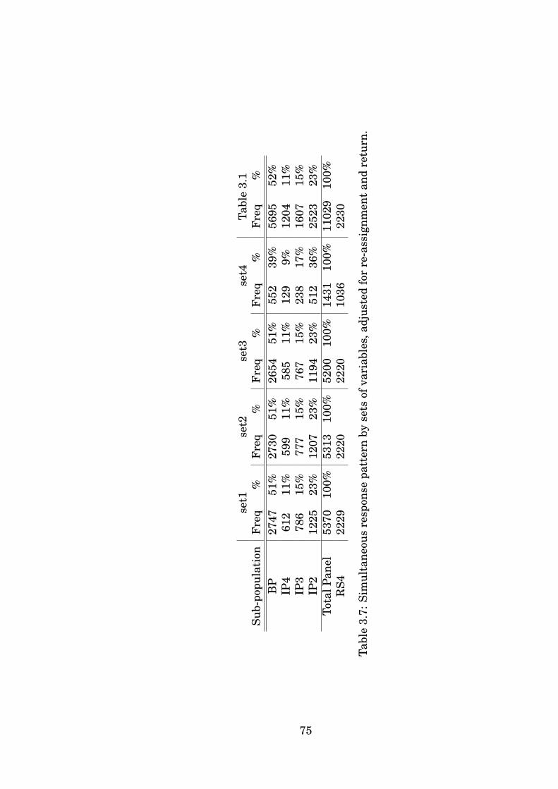
set1
set2
set3
set4
Tabl
e3.
1Su
b-po
pula
tion
Fre
q%
Fre
q%
Fre
q%
Fre
q%
Fre
q%
BP
2747
51%
2730
51%
2654
51%
552
39%
5695
52%
IP4
612
11%
599
11%
585
11%
129
9%12
0411
%IP
378
615
%77
715
%76
715
%23
817
%16
0715
%IP
212
2523
%12
0723
%11
9423
%51
236
%25
2323
%To
talP
anel
5370
100%
5313
100%
5200
100%
1431
100%
1102
910
0%R
S422
2922
2022
2010
3622
30
Tabl
e3.
7:Si
mul
tane
ous
resp
onse
patt
ern
byse
tsof
vari
able
s,ad
just
edfo
rre
-ass
ignm
ent
and
retu
rn.
75

set1
set2
set3
set4
Tabl
e3.
2Pe
rsis
tenc
eF
req
%F
req
%F
req
%F
req
%F
req
%w
ave
153
7053
1352
0014
3111
029
wav
e1
-wav
e2
4145
77%
4106
77%
4006
77%
919
64%
8506
77%
wav
e2
-wav
e3
3359
81%
3329
81%
3239
81%
681
74%
6899
81%
wav
e3
-wav
e4
2747
82%
2730
82%
2654
82%
552
81%
5695
83%
Tabl
e3.
8:Pe
rsis
tenc
era
tes
for
core
mem
bers
ofth
eE
LSA
pane
l,ad
just
edfo
rre
-ass
ignm
ent
and
retu
rn.
76

3.3 Preliminary Evidence of Selection
Many panel data analyses ignore the attrition problem by using only the bal-
anced panel. If the people that continue to respond are different from the
people that leave the panel with respect to the variables of interest, this leads
to selection bias. As a preliminary analysis, sample means of sub-populations
with different response patterns can be compared. Table 3.9 reports differ-
ences in average income. As this variable is continuously measured, the re-
gression results in the table are easy to interpret. For labor market status,
the variable of interest, a nonlinear model would be required. Previous analy-
sis has shown that income and wealth are key financial determinants of when
people retire (Blundell et al. (2002)).
Table 3.9 shows cross-sectional regressions of income on waves1 and waves2,
binary variables that indicate the duration of panel-membership. The vari-
able wave1 equals 1 if the individual dropped out of the panel after one wave,
and zero otherwise. Wave2 equals one in case of two consecutive waves of
participation. Only the first three waves of the ELSA panel are used here, as
the variable income is not yet available for the fourth wave. The results in the
first regression column show that, compared to the balanced panel, average
net weekly income is significantly lower in IP2. With 91.97, the difference is
substantial. The sample average in IP3 is 73.13 lower than in the balanced
panel. By setting these mean-comparisons up as OLS regressions, other re-
gressors can be included. This enables us to investigate whether the differ-
ences in income persist when more similar individuals are compared within
the sub-populations defined by the response patterns. After inclusion of the
77

inco
me
inco
me
inco
me
inco
me
coef
fs.
e.co
eff
s.e.
coef
fs.
e.co
eff
s.e
cons
396.
716.
5061
2.83
15.4
129
4.71
10.6
149
8.67
18.0
9w
aves
1-9
1.97
18.3
2-4
9.66
16.5
6-5
5.52
18.5
6-4
2.63
16.8
1w
aves
2-7
3.13
17.3
0-4
0.81
15.0
1-3
3.10
17.4
7-2
4.06
15.2
2ph
ealt
h(p
oor)
-56.
2424
.18
-4.5
321
.41
phea
lth
(fai
r)-5
1.70
15.7
0-9
.12
13.9
5w
ork
178.
2916
.13
181.
3914
.60
age
(50-
59)
120.
1817
.46
40.7
416
.16
age
(60-
69)
91.7
213
.92
42.1
512
.44
mhe
alth
-74.
6815
.70
-30.
6014
.04
mal
e4.
7310
.43
-2.1
710
.44
sing
le-1
84.3
011
.31
-161
.00
11.4
4ed
uc(g
ce,c
se)
-117
.52
15.0
0-1
20.6
714
.90
educ
(no)
-247
.13
13.1
0-2
01.1
013
.47
educ
(oth
er/fo
reig
n)-2
07.6
620
.21
-180
.79
20.2
0m
t1ch
ild-2
5.52
11.7
4-3
.06
11.7
9
Tabl
e3.
9:R
egre
ssio
nsof
inco
me
ondi
ffer
ent
sets
ofex
plan
ator
yva
riab
les
and
attr
itio
nin
dica
tors
.
78

time-constant variables, the differences are still significant, as the second col-
umn of Table 3.9 shows. The same result is obtained when the time-constant
variables are replaced by time-varying ones. The last column shows that, if
both sets of variables are included, average income in IP3 is no longer signif-
icantly different from average income in the balanced panel. This suggests
that an attrition model that corrects for selection on observables is required.
The differences in average income between IP2 and the balanced panel, indi-
cated by the significance of waves1, hints at potential selection on unobserv-
ables.
3.4 Attrition Models
In each wave, a panel study obtains responses on a vector of variables Z. For
each individual, the vector of responses in wave t is denoted by Zt. The bi-
nary indicator Dit takes the value 1 if responses are obtained for individual i
in wave t. For simplicity, I assume that for all individuals approached in the
first wave responses were obtained. In the ELSA panel this assumption is rea-
sonable (details can be found in the documentation). The presence of attrition
in a panel with two waves implies that the distribution f(Z2|Z1, D2 = 0) is not
observed. Attrition can be modelled by restricting the conditional probability
of observation in both waves. This observation probability would be unre-
stricted if P (D2 = 1|Z1, Z2) = G(k(Z1, Z2)), where G denotes some cdf function
and k denotes the index function. For example, in a logit model, G would
be the cdf of the logistic distribution and k would be a linear function of the
variables in Z1 or Z2. Any particular choice of the index function corresponds
79

with a particular unobserved distribution f(Z2|Z1, D2 = 0). Attrition models
can hence be described by the restrictions they place on the index function k.
What follows is a discussion of the four most commonly used attrition models
for panels with two waves.
Ignoring the attrition problem amounts to assuming that the index function
is a constant, P (D2 = 1|Z1, Z2) = G(k0). In other words, the probability of
observation does not vary with Z1 or Z2. The population distribution solution
implied by the assumption of MCAR attrition, fMCAR(Z1, Z2), then equals the
balanced panel distribution f(Z1, Z2|D2 = 1). Any complete-cases analysis of
panel data implicitly assumes MCAR.
A less restrictive alternative is Missing At Random (MAR). This attrition
model assumes that P (D2 = 1|Z1, Z2) = G(k0 + k1(Z1)). The observation prob-
ability is allowed to vary with Z1 in arbitrary ways, via the unrestricted func-
tion k1, but cannot depend on Z2. As Z1 is observed for all individuals in the
panel, MAR is called ignorable. In the econometrics literature it is sometimes
referred to as selection on observables (Fitzgerald and Moffitt (1998)).
Non-ignorable models allow for selection on unobservables in that they have
the observation probability depend on the partially observed Z2. An example
of this is provided by the attrition model suggested by Hausman and Wise
(1979): P (D2 = 1|Z1, Z2) = G(k0 + k2(Z2)). Note that HW admits selection on
unobservables but at the same time rules out selection on observables. Both
the MAR and HW attrition models are nonparametrically just-identified: they
are identified and have no testable implications and are hence observationally
equivalent.
80

If a refreshment sample is available in the second wave, Hirano et al. (2001)
show that the Additively Non-ignorable (AN) attrition model identifies the
population distribution, with observation probability P (D2 = 1|Z1, Z2) = G(k0+
k1(Z1) + k2(Z2)). The AN model admits Non-ignorable attrition and does not
rule out selection on observables. This model is generalized to panels with
any number of waves in chapter 2 of this thesis. The resulting Sequential
Additively Non-ignorable (SAN) attrition model imposes restrictions on the
attrition hazards to achieve just-identification:
P (Dt = 1|Dt−1 = 1, . . . , D1 = 1) = G(k0 + k(Z1, . . . , Zt−1) + k(Zt)).
where the functions G denotes a cdf, e.g a logit. In a four wave panel where
Zt consists of a single binary indicator, these attrition hazards reduce to
P (D2 = 1|Z2) = G(α0 + α1Z1 + α2Z2) (3.1)
P (D3 = 1|D2 = 1, Z3) = G(β0 + β1Z1 + +β2Z2 + β12Z1Z2 + β3Z3) (3.2)
P (D4 = 1|D3 = 1, Z4) = G(γ0 + γ1Z1 + γ2Z2 + γ3Z3 (3.3)
+ γ12Z1Z2 + γ13Z1Z3 + γ23Z2Z3 + γ4Z4). (3.4)
3.5 Estimation of the SAN Attrition Model
For the ELSA panel, currently only a fourth wave refreshment sample is
available.3 Consequently, there is no good reason to include a non-ignorable3As mentioned earlier, no complete refreshment samples were obtained in previous waves.
In the third wave ELSA did collect a refreshment sample, but this sample included 50-53 year
81

attrition model for attrition in the second wave. Indeed, any HW attrition
model has an observationally equivalent solution derived from MAR (Hirano
et al. (2001), Bhattacharya (2008)). For the same reason, attrition in the third
wave can take the form of MAR.4 For the analysis of attrition in the ELSA
panel this is unfortunate, given the results discussed in section 3.3. As in the
fourth wave a refreshment sample was collected, an AN model for attrition in
the fourth wave identifies the parameters of interest.
Estimation of the SAN model can proceed by the weighted GMM estimator
proposed in chapter 2. This estimator chooses weights that are such that the
weighted balanced panel is consistent with all the information in the panel
and the refreshment samples. Estimation of the weights is simplified by
matching on a set of moments instead of on the full marginal distributions
obtained from the refreshment samples. The SAN solution can be approxi-
mated by matching on a large set of such moments.
3.5.1 Moment Conditions
The parameters of interest are the probabilities of transition into inactivity
in the second, third and fourth waves, respectively. Let Zt denote the value
taken by the binary variable work in wave t. This variable takes the value one
for individuals that are active in the labor market and zero otherwise. Theolds only. This was done to “refresh” the cohort of youngest core members in the ELSA panel.In the first wave, the youngest eligible core member was approximately aged 50. In the thirdwave these individuals were hence aged 54. In wave 4 refreshment sample members of allcohorts were sampled and as such auxiliary information was gathered about all age cohortscontained in the original panel. It is for this reason that we only consider this sample as arefreshment sample.
4Section 7 proposes the GHW model for attrition, which allows for non-ignorability ofattrition in the third wave under some additional restrictions.
82

transition probabilities can be characterized as the solutions of the following
moment equations:
E[I(Z2 = 0|Z1 = 1)− θ1] = 0
E[I(Z3 = 0|Z2 = 1)− θ2] = 0
E[I(Z4 = 0|Z3 = 1)− θ3] = 0,
where I(A) equals 1 if A holds and is zero otherwise. In the absence of attri-
tion, method of moments estimates of the transition probabilities θ1, θ2 and
θ3 can be obtained by calculating the relevant sample fractions. To correct
for the attrition in the ELSA panel the weighted balance panel must be used.
Weights that allow for SAN attrition use (3.4), adding 16 parameters to esti-
mate. Imposing MAR in the second and third wave corresponds the restric-
tions α2 = β3 = 0. The binary nature of Z implies that only first moments
need to be matched.
3.5.2 Estimation Results
The estimation results are reported in Table 3.10. For brevity, the attrition
parameter estimates are categorized in three categories: selection on observ-
ables in wave t indicates that one or more coefficients of Z in earlier waves
are significantly different from zero. This implies that the attrition problem
in that wave cannot be ignored, and MCAR estimates are potentially mislead-
ing. Selection on unobservables in wave t implies that the coefficient of Zt was
significant. A selection on observables (MAR) model is not sufficient in that
83

case, and AN estimates are more credible.
The transition probability estimates show that the MCAR underestimates the
transition probabilities in the second and third wave. This suggests that in-
dividuals that exit the labor market are under-represented in the balanced
panel. In other words, individuals that exit the labor market are more likely
to attrit. A possible explanation for this result is that individuals that retired
relatively recently are more likely to have moved. It could also be that both
attrition and retirement are related to health.
The results can also be linked to the analysis in section (3.3). There it was
shown that the average income in the balanced panel is relatively high, when
compared to IP2 and IP3. Individuals that earn more tend to prefer a phasing
out approach to retirement (Banks et al. (2010)). Phasing out means that
transition to part-time work precedes transition into retirement. As Zt equals
one for both part-time and full-time workers, working less hours does not
correspond to a transition in Z. Less transitions will hence be observed in
the balanced panel, where average income is relatively high. A conditional
analysis could be more revealing. Such an analysis would, however, involve
many more parameters and is beyond the scope of this chapter.
Not surprisingly, the attrition results show evidence of selection on observ-
ables in all waves where attrition occurs. The AN model that uses the infor-
mation contained in the fourth wave refreshment sample does not indicate
non-ignorability of the attrition.
84

MC
AR
MA
R-M
AR
-MA
RM
AR
-MA
R-A
NT
rans
itio
nco
eff
s.e.
coef
fs.
e.co
eff
s.e.
wav
e1-
wav
e2
(θ1)
0.17
80.
026
0.21
30.
031
0.21
20.
028
wav
e2
-wav
e3
(θ2)
0.16
30.
029
0.22
10.
034
0.20
00.
031
wav
e3
-wav
e4
(θ3)
0.23
70.
032
0.21
80.
042
0.22
40.
040
Att
riti
onw
ave
num
ber
type
ofse
lect
ion
wav
e2
obse
rvab
les
-ye
sye
sun
obse
rvab
les
--
-w
ave
3ob
serv
able
s-
yes
yes
unob
serv
able
s-
--
wav
e4
obse
rvab
les
-ye
sye
sun
obse
rvab
les
--
no
Tabl
e3.
10:E
stim
ates
oftr
ansi
tion
prob
abili
ties
into
inac
tivi
tyun
der
seve
rala
ttri
tion
mod
els.
85

3.6 Non-ignorable Attrition in Waves Without
Refreshment Samples
If attrition is counteracted by collecting refreshment samples, the SAN attri-
tion model identifies the population distribution and selection on unobserv-
ables can be admitted. A potential weakness of the analysis in section 3.5
is that in the ELSA panel no such refreshment samples have been collected
in waves two and three. By exploiting the moment conditions in a slightly
different way, selection on unobservables can however be allowed for. In this
section I propose the Generalized Hausman and Wise (GHW) attrition model
that can be used for that purpose. It will be shown how it can accommodate
potential selection on unobservables due to attrition in the third wave of the
panel.
3.6.1 The Generalized Hausman and Wise Attrition Model
The SAN attrition model maintains two sets of restrictions on the third wave
attrition hazard, sequential attrition and additive non-ignorability. Below, I
clarify the nature of these assumptions in our binary application. The popu-
lation distribution f(Z1, Z2, Z3) has 8 parameters in this case. Attrition can be
taken into account by adding a model for P (D1 = 1, D2 = 1, D3 = 1|Z1, Z2, Z3).
Sequential attrition then implies that this probability equals
P (D1 = 1, D2 = 1, D3 = 1|Z1, Z2, Z3) = Π3t=2P (Dt = 1|Dt−1 = 1, . . . , D1, Z1, . . . , Zt).
86

The two attrition hazards can be parameterized as
P (D2 = 1|D1 = 1, Z1, Z2, Z3) = G(γ0 + γ1Z1 + γ2Z2 + γ12Z1Z2) (3.5)
P (D3 = 1|D2 = 1, Z1, Z2, Z3) = G(δ0 + δ1Z1 + δ2Z2 + δ3Z3 + δ12Z1Z2 (3.6)
+δ13Z1Z3 + δ23Z2Z3 + δ123Z1Z2Z3), (3.7)
resulting in an additional 12 parameters. Models that have no testable im-
plications can be obtained by requiring that the pair (f(Z1, Z2, Z3), P (D1 =
1, D2 = 1, D3 = 1|Z1, Z2, Z3)) be consistent with the observable distributions
f(Z1, Z2, Z3|D1 = 1, D2 = 1, D3 = 1) from the balanced panel, f(Z1, Z2|D2 =
1, D3 = 0) from IP3, f(Z1|D2 = 0) from IP2, as well as the response fractions
P (D2 = 1) and P (D3 = 1|D2 = 1). These provide 14 restrictions, implying
that another 6 restrictions are needed to identify the model. The SAN model
imposes
γ12 = δ13 = δ23 = δ123 = 0.
The remaining two restrictions are obtained by requiring consistency with
P (Z2 = 1) and P (Z3 = 1), obtainable from second and third wave refreshment
samples. As no refreshment samples are available for the ELSA panel in the
second and third wave, the latter two restrictions cannot be imposed here.
Identification can be achieved by fixing γ2 and δ3 at a particular value, as pro-
posed by Rotnitzky et al. (1998). Alternatively, we may impose restrictions on
the joint population distribution to reduce the number of parameters. There
is a considerable literature (Baker and Laird (1988), Baker (1995), Chambers
and Welsh (1993), Conaway (1993), Fitzmaurice et al. (1995)) that imposes
a mixture of distributional assumptions on the population distribution and
87

functional form assumptions on the attrition probabilities. However, leaving
the population distribution unrestricted has the advantage that the identifi-
cation becomes independent of the population model used. I therefore impose
the restrictions γ2 = γ12 = 0, corresponding to MAR attrition in the second
wave. The remaining 4 restrictions can be obtained by requiring that the third
wave attrition does not depend on Z1, implying that δ1 = δ12 = δ13 = δ123 = 0.
For the general case, this corresponds to a first order Markov assumption on
the third period attrition hazard:
P (D3 = 1|D2 = 1, D1 = 1, Z1, Z2, Z3) = G(k0 + k1(Z2, Z3)).
I will refer to this model as the Generalized Hausman and Wise (GHW) model.
Its advantage is that it allows for non-ignorable attrition in third wave with-
out requiring a refreshment sample. The disadvantage is that it does so by
ruling out some, but not all, forms of selection on observables. This con-
trasts with the Hausman and Wise model in the second wave, that rules out
all forms of selection on observables to achieve non-ignorability. It must be
stressed, though, that, even in the third wave, an observationally equivalent
solution can be derived from MAR.
3.6.2 Estimation Results for the GHW Model
The estimates using the GHW model are shown in Table 3.11. To facilitate
comparison, the MAR estimates from Table 3.10 are repeated in the first col-
umn of this table.
88

MA
R-M
AR
-MA
RM
AR
-GH
W-G
HW
MA
R-G
HW
-AN
Tra
nsit
ion
coef
fs.
e.co
eff
s.e.
coef
fs.
e.w
ave
1-w
ave
2(θ
1)
0.21
30.
031
0.19
80.
034
0.20
10.
029
wav
e2
-wav
e3
(θ2)
0.22
10.
034
0.18
90.
032
0.19
60.
032
wav
e3
-wav
e4
(θ3)
0.21
80.
042
0.22
10.
041
0.22
50.
044
Att
riti
onw
ave
num
ber
type
ofse
lect
ion
wav
e2
obse
rvab
les
yes
yes
-un
obse
rvab
les
--
-w
ave
3ob
serv
able
sye
sye
sye
sun
obse
rvab
les
-no
now
ave
4ob
serv
able
sye
sye
sye
sun
obse
rvab
les
-no
no
Tabl
e3.
11:E
stim
ates
oftr
ansi
tion
prob
abili
ties
into
inac
tivi
tyus
ing
the
MA
RG
HW
attr
itio
nm
odel
.
89

The estimates of the transition probabilities are similar to those in Table 3.10.
The MCAR attrition model is rejected in favor of selection on observables. No
evidence is found for selection on unobservables. The results in Table 3.10
and Table 3.11 can be summarized as follows: although the attrition in the
ELSA panel cannot be ignored, it can be dealt with by maintaining selection
on observables.
3.7 Summary and Conclusion
In this chapter, estimates were obtained for the probability of transition into
inactivity for elderly people using the English Longitudinal Study of Ageing
(ELSA). The aim of the study was to investigate if the estimates are affected
by the potentially nonrandom attrition in the ELSA panel. By exploiting the
information available in the fourth wave refreshment sample, attrition in the
fourth wave could be permitted to be non-ignorable through the use of the
SAN attrition model. Attrition in earlier waves was restricted to MAR.
The estimates show that ignoring the attrition by using only the balanced
panel, leads to underestimation of the transition probabilities. This suggests
that individuals that exit the labor market are more likely to attrit. There
is insufficient evidence of non-ignorable attrition in the fourth wave. Non-
ignorability was ruled out by the attrition model in the second and third wave.
The Generalized Hausman and Wise attrition model was proposed as an al-
ternative to MAR in the third wave. The advantage of this model is that it
allows for non-ignorable attrition in the absence of refreshment samples. The
90

disadvantage is that it does so by ruling out some, but not all, forms of selec-
tion on observables. The estimates that were obtained were not suggestive of
non-ignorable attrition in the third wave.
91

Appendix
To ensure that the study is reproducible, Table 3.12 lists the variables that
were used. Table 3.13 shows the derived variables.
92

Vari
able
nam
eD
escr
ipti
onC
odin
gT
ime-
cons
tant
Hea
lth
hehe
lfse
lf-r
epor
ted
heal
thpo
or,f
air,
good
,ver
ygo
od,e
xcel
lent
nohe
illlo
ngst
andi
ngill
ness
es?
yes,
nono
helim
Do
thes
elim
ityo
urac
tivi
ties
?ye
s,no
nops
ceda
depr
esse
dla
stw
eek?
yes,
nono
Wor
kw
pdes
wor
kre
tire
d,em
pl.,
self
-em
pl,u
nem
pl,
nodi
sabl
,loo
kaf
ter
hom
e,se
mi-
reti
red
Inco
me
toti
nc_b
uto
taln
etin
com
ew
eekl
yno
nett
otw
_bu
tota
lnet
(non
-pen
sion
)wea
lth
poun
dsno
Oth
erin
dage
rag
eye
ars
nodh
sex
resp
onde
nt’s
sex
mal
e,fe
mal
eye
sdi
mar
mar
ital
stat
usne
ver
mar
ried
,mar
ried
,re-
mar
ried
,ye
sle
gally
sepa
rate
d,di
vorc
ed,w
idow
edsc
ptpa
5ho
liday
abro
adin
past
year
yes,
nono
scor
g9N
ota
mem
ber
ofcl
ubs
yes,
nono
edqu
alH
ighe
sted
uc.q
ual.
degr
ee,h
ighe
red
uc,g
ce,c
se,o
ther
,no
yes
sem
i-sk
man
,uns
km
an,a
rmed
forc
esdh
nch
#liv
ing
non-
res
child
ren
0-13
yes
Table 3.12: Variable descriptions of the variables used in the analysis.
93

Vari
able
nam
eD
escr
ipti
onD
eriv
edfr
omC
odin
gT
ime-
Con
stan
tph
ealt
hSe
lf-r
epor
ted
phys
ical
heal
thhe
helf,
hege
nhpo
or,f
air,
good
nolo
ngill
Lon
gsta
ndin
glim
itin
gill
ness
heill
,hel
imye
s,no
nom
heal
thde
pres
sed
duri
ngla
stw
eek?
psce
daye
s,no
now
ork
Act
ive
inth
ela
bor
mar
ket
wpd
esye
s,no
noin
com
eto
taln
etw
eekl
yin
com
eto
tinc
_bu
inpo
unds
now
ealt
hto
taln
et(n
on-p
ensi
on)w
ealt
hne
ttot
w_b
uin
poun
dsno
age
Age
inda
ger
inye
ars
noag
ecA
geca
tego
ryin
dage
r50
-59,
60-6
9,70
+no
mal
eR
espo
nden
tis
mal
edh
sex
yes.
noye
ssi
ngle
Not
mar
ried
orno
tre
-mar
ried
dim
arye
s,no
yes
holid
ayH
olid
ayab
road
last
year
scpt
pa5
yes,
nono
club
sM
embe
rof
any
club
s?sc
org0
9ye
s,no
noed
ucH
ighe
stat
tain
edqu
alifi
cati
oned
qual
high
er/g
ce,c
se/o
ther
/no
yes
mt1
child
>1liv
ing
(non
-res
)chi
lddh
nch
yes,
noye
s
Table 3.13: Variable descriptions of derived variables.
94

Chapter 4
EM estimation of Panel data
Models with Nonignorable
Attrition and Refreshment
Samples
4.1 Introduction
Panel-data are obtained by repeatedly observing units (e.g. firms, countries or
households). Compared to that of a single cross-section or a single time series,
the use of panel data permits the identification of more elaborate models. At
the same time, missing data problems often become more severe, especially
unit non-response. Indeed, in many panel surveys the fraction of units that
leave the panel at a certain time period is non-negligible. This type of non-
95

response is called attrition. When not taken into account, attrition can be
particularly harmful if it is related to the variables of interest. In that case
the attrition is called selective. If the attrition in a particular time-period is
related to the value contemporaneously taken by some variable of interest it
is called nonignorable.
Until recently, tests for the selectivity of attrition as well as estimation meth-
ods meant to correct for the resulting bias were based on stochastic censoring
models of response behaviour. A joint (conditional) model for the outcome
variable of interest and the presence of the unit in the current wave of the
panel is specified. Often, the outcome variable is assumed to relate to the con-
ditioning variables by means of some standard panel data regression model,
e.g. a random effect model. Possible non-ignorability of the attrition is ad-
mitted by allowing for correlation between the unobserved components of this
joint model, see e.g. Hausman and Wise (1979), Ridder (1990), Ridder (1992)
and Verbeek and Nijman (1992). Identification of these models relies on either
the availability of an instrument or on functional form restrictions. Moreover,
different panel data regression models give rise to different correlation struc-
tures.
Hirano et al. (2001) have proposed a way out of this deadlock by using of re-
freshment samples. These are random samples from the population of inter-
est. This additional data source allows for the nonparametric just-identification
of the population distribution of the outcome variables in a panel of two waves
under weak assumptions on the response probabilities. Their results are gen-
eralized to panels with any number of waves in chapter 2 of this thesis. The
chapter also proposes a weighted GMM estimator to estimate parameters that
96

solve a set of moment equations in the population. The SAN attrition model
implies a population distribution solution that is consistent with all the in-
formation in the panel and the refreshment samples. Any particular model,
e.g. a linear regression model relating Z to X, imposes a restriction on this
distribution and therefore inherits this correction.
In this chapter, I propose an Expectation-Maximization (EM) algorithm for
maximum likelihood to estimate the parameters of a generic parametric panel
data model under SAN attrition. The algorithm is non-standard because the
SAN model allows for non-ignorable attrition. Almost all EM algorithms pro-
posed in the missing data literature require Missing At Random. In addition,
the values taken by regressor variables are usually assumed to be constant
over time. I do not make this assumption in this chapter.
The parametric nature of maximum likelihood implies that more restrictions
are made than strictly necessary for nonparametric identification. A GMM
approach would be less restrictive. Moreover, when the likelihood is specified,
estimation could proceed by using the expected score in the GMM approach.
However, the EM algorithm proposed in this chapter has the advantage that
it can be used in cases where the score function is hard to obtain.
The outline of the chapter is as follows. Section 4.2 considers a two-period
panel and discusses the Additively Non-ignorable attrition model of Hirano
et al. (2001) and its specializations. Section 4.3 discusses the SAN generaliza-
tion. Section 4.4 describes the advantages of EM over a direct likelihood ap-
proach. The EM algorithm for discrete time-varying regressors is presented
in section 4.5. The discreteness assumption is then relaxed in section 4.6.
97

Section 4.7 provides an interpretation of the algorithm as a weighted MAR
procedure. The final section comments and concludes.
4.2 Identification of Population Models with
Attrition and Refreshment Samples
This section outlines the attrition problem, the sampling process under con-
sideration and the identifying assumption imposed on the attrition process.
In the sequel, Z is the variable (possibly a vector) of interest, i.e. the depen-
dent or endogenous variable1, and X is a (vector of) independent or exogenous
variable(s). We consider a panel of two waves that we label as 1 and 2. The
joint distribution of Z1, Z2 given X in the population has density
f(Z1, Z2|X) (4.1)
A model, e.g. a linear regression model that relates Z1 and Z2 to X (or Z1 to X
and Z2 to Z1 and X if one considers a model with lagged dependent variables),
is a restriction on this joint density that may involve a vector of parameters
θ.
We assume that we always observe X and Z1, but that as a consequence of
attrition we fail to observe Z2 for some fraction of the population. Let D be1More precisely, a vector Z may also contain time-varying covariates that are not com-
pletely observed, as will be discussed in section 4. The characterizing feature of variablesthat are contained in Z is that they are only partially observed for some subjects due toattrition. The set of variables that are observed in every time-period for every subject arecontained in X. For ease of exposition, for the moment it is assumed that only endogenousvariables have missing values.
98

the indicator of the observation of Z2, with D = 1 if Z2 is observed and with
D = 0 if it is not observed. Then our observation process allows us to recover
f(Z1|X) (4.2)
f(Z1, Z2|X,D = 1) (4.3)
To isolate the attrition problem, note that the observation process is unin-
formative with respect to f(Z2|Z1, X,D = 0). Therefore, without additional
information the population distribution is not identified2. To model attrition
we specify a model for the observation probability
Pr(D = 1|Z1, Z2, X) = G(k(Z1, Z2, X)) (4.4)
with G being a (prespecified) c.d.f. of some continuous distribution, e.g. the
logistic or standard normal, and k being some real-valued index-function.
In many panel studies attrition does not come as a surprise. Indeed, the
designers anticipate attrition and, because they want to keep the number of
units approximately constant, they ’refresh’ the panel by ’replacing’ the units
that are lost by new (randomly selected) units. In our notation this amounts
to observing the distribution of Z2 (given X)
f(Z2|X) (4.5)2This does not mean that the sampling process is completely uninformative with respect
to (4.1). One may be able to put bounds on the set of distributions that are consistent withthe available information. See Manski (1995) for details.
99

The key result in Hirano et al. (2001) is that if we restrict k to be additive in
Z1 and Z2,
k(Z1, Z2, X) = k0(X) + k1(Z1, X) + k2(Z2, X) (4.6)
then we can uniquely identify the population distribution in (4.1) (and hence
any model that is a restriction of this distribution). Hirano et al. (2001) refer
to (4.4) with restriction (4.6) as the Additively Non-ignorable (AN) model. The
motivation for identification by additive non-ignorability is that AN estimates
can be interpreted as minimizing the discrepancy with the balanced panel
estimates among the set of estimates that satisfy the restrictions imposed by
the refreshment sample and the distribution f(Z1), observable from the panel.
Hirano et al. (2001) show that this is a case of just identification; the AN
restriction does not impose any testable restrictions on distributions of ob-
servables.
Before we relate the AN restriction to other restrictions proposed in the litera-
ture, it is convenient to first consider a more restrictive version of the attrition
process. Suppose, therefore, that that the functions k0, k1 and k2 are known
to be linear in X, Z1 and Z2, respectively. Moreover, assume that G is the
standard normal distribution function Φ. This reduces (4.4) to
Pr(D = 1|Z1, Z2, X) = Φ(α′1Z1 + α′2Z2 + α′XX)) (4.7)
with the α’s denoting parameter vectors. In what follows, this model is re-
ferred to as the linear AN assumption. Now we relate this assumption to the
ones most commonly used in practice. To facilitate this discussion, first note
100

that
Pr(Z1, Z2|X) = Pr(Z1, Z2|X,D = 1)Pr(D = 1|X)
Pr(D = 1|Z1, Z2, X). (4.8)
In the terminology of Little and Rubin (1987), the most stringent assumption
is Missing Completely At Random (MCAR). This assumes that the observed
distribution equals the population distribution. It is apparent from (4.8) that
this can be denoted as D⊥Z1, Z2|X or k1(Z1, X) = k2(Z2, X) = 0 in (4.6), which
implies α1 = α2 = 0 in (4.7). Essentially, this states that, although there
are data missing, there is no missing data problem. Inference based on com-
pletely observed units does not lead to biased results in this case. Indeed, any
empirical study that disregards incomplete observations implicitly assumes
MCAR.
The second, and most popular, assumption is called Missing At Random (MAR).
Although tolerating a non-random sample from the population distribution,
this requires random draws from the conditional distribution of the (not com-
pletely observed) Z2 given the (completely observed) Z1 and X. This identifies
the joint population distribution by assuming D⊥Z2|X or k2(Z2, X) = 0 in
(4.6), which implies α2 = 0 in (4.7). This assumption is attractive for two rea-
sons. First, it identifies the population distribution non-parametrically from
the unbalanced panel without the need of a refreshment sample. Second,
under certain conditions the attrition process is ignorable when inference is
likelihood-based. Specifications of response models that obey the MAR as-
sumption end up cancelling from the likelihood. Therefore, no explicit speci-
fication of the response model is necessary, other then restricting it to belong
to the MAR-class of models. Hence the term ignorability.
101

In observational studies it is often not appropriate to assume ignorability of
the attrition process. Hausman and Wise (1979) developed an attrition model
that corresponds with α1 = 0 in (4.7). An obvious generalization is D⊥Z1|X or
k1(Z1, X) = 0 in (4.6). The attrition is therefore allowed to depend on values
taken by the variables of interest that are not always observed. As a conse-
quence, even the observed conditional distribution is a distorted version of its
population counterpart. This type of attrition is called non-ignorable.
All assumptions discussed above are nested within the AN assumption. The
refreshment sample provides just enough identifying power to permit the at-
trition process to be non-ignorable (unlike MAR) while allowing MAR as a
nested sub-model (unlike HW). The next section discusses the generalization
of the AN model to panels with more than two waves.
4.3 Identification of Population Models With More
Than Two Periods
Longitudinal studies often continue for more than two periods. In this sec-
tion the Sequential Additively Non-ignorable class of attrition models is dis-
cussed. This model extends the AN model to multi-wave panels. First, we
have to be precise about the sampling scheme. Consider a panel with Np sub-
jects, indexed by i, that are approached for T periods. Subject i responds for
Ti periods, and, when Ti < T , will not be approached in the remaining peri-
ods. The set of observations that belong to subjects that responded in all T
time periods is referred to as the Balanced Panel (BP). The set of observations
102

with unit non-response from a certain period onwards is referred to as the In-
complete Panel (IP). More specifically, IPt is the subset of IP with attrition
occurring in period t, with 2 ≤ t ≤ T . The panel, consisting of the balanced
panel and the incomplete panels, has Np observations. In obvious notation,
we have Np = NCP + NIP with NIP = ΣTt=2NIPt. The absence of return im-
plies a missing data pattern in the panel that is monotone (Little and Rubin
(1987)). Monotonicity disappears after inclusion of the refreshment samples.
In multi-wave panels attrition occurs several times. A random refreshment
sample is drawn in each wave, starting from the second wave. Each refresh-
ment sample yields NRSt additional observations. In total, the refreshment
samples contain NRS = ΣTt=2NRSt additional subjects.
Our objective is to combine the balanced panel, the incomplete panel and
the refreshment samples with a structure imposed on the attrition process
so as to identify the joint population distribution of the variables of interest,
f(Z1, . . . , ZT |X). The attrition process is described by the distribution of the T
dimensional vector of binary variables (Di1, . . . , DiT ) conditional on the values
taken by the variables of interest Z1, . . . , ZT and a set of covariates X. A key
assumption for identification is Sequential Attrition (SA). This assumption
implies
Pr D1 = 1, . . . , DT = 1|Z1, . . . , ZT , X = ΠTt=2 Pr Dt = 1|Dt−1 = 1,Zt, X (4.9)
omitting the subject index i. Boldfaced symbols like Zt, denote the history
of the variable in question, i.e. the t-vector (Zt, . . . , Z1). Decomposition (4.9)
states that the attrition hazard in period t does not depend on the values
taken by the variables of interest at any period later than t.
103

It suffices to illustrate the identification result in chapter 2 for panels with
three waves. Given the identification of f(Z1, Z2|X), from the AN model of
Hirano et al. (2001), identification of f(Z1, Z2, Z3|X) requires identification of
f(Z3|Z2, Z1, X). Since there have now been two realizations of dropout, the ob-
servation process is uninformative about two distributions, namely f(Z3|Z1, Z2, D2 =
1, D3 = 0, X) and f(Z3|Z1, Z2, D2 = 0, D3 = 0, X). Sequential attrition implies
f(Zt|Zt−1,Dt−1 = 1, X) = f(Zt|Zt−1, X). (4.10)
The identifying power of the sequential attrition assumption resides in the
implication that the unobserved distribution f(Z3|Z1, Z2,W2 = 0,W3 = 0, X) is
not informative for the identification of f(Z3|Z1, Z2, X). This suggests that the
identification of f(Z1, . . . , ZT |X) can be pursued by sequentially identifying
f(Zt|Zt−1, X) for 2 ≤ t ≤ T . For each value of t there is one observed distribu-
tion f(Zt|Zt−1,Dt = 1, X), effectively one unobserved distribution f(Zt|Zt−1,Dt−1 =
1, Dt = 0, X) and a refreshment sample identifying f(Zt|X). This resembles
the situation studied in Hirano et al. (2001), which suggests that the SAN at-
trition model is identified. This is formally shown in chapter 2. The definition
of the SAN model is:
Definition 6. The sequence of attrition hazards pt = Pr Dt = 1|Dt−1 = 1,Zt, X
for 2 ≤ t ≤ T obey the Sequential Additively Non-ignorable attrition model if
pt = G(k0(X) + k1(Zt−1, X) + k2(Zt, X)),
where k0(X), k1(Z1, Z2) and k2(Z3) are arbitrary squared Lebesgue integrable
functions. They are normalized to equal zero in some point in the support of
104

(Zt, X) to allow for the inclusion of the constant k0.
4.4 EM-algorithm For General Panel Data
Models
This section describes maximum likelihood estimation of SAN models with an
EM algorithm. I argue that the algorithm has clear advantages over a direct
likelihood approach. The algorithm is described in terms of generic densities
and is hence generally applicable.
4.4.1 Direct Likelihood
Maximum likelihood estimation usually involves numerical optimization over
the parameter space. When a model incorporates some missing data mecha-
nism to reflect that the data are only partially observed, the simultaneous
log-likelihood is often more difficult to optimize; the missing data process
may affect the global concavity that is present in the original log-likelihood.
Consider the log-likelihood of an observation in the balanced panel when the
panel has two waves:
lnLBP = ln f(Z1, Z2|X)+ ln Pr(D = 1|Z1, Z2, X) (4.11)
In the incomplete panel, Z2 is not observed and therefore needs to be inte-
grated out. Additional notation is needed to describe the implications. The
characterizing feature of a variable that is contained in Z is that it is only
105

partially observed for some subjects due to attrition. The set of variables that
are observed in every time-period for every subject are contained in X. This is
a natural division of variables when discussing attrition in panel data in gen-
eral terms. In applications, however, it is customary to distinguish between
variables of interest and explanatory variables or covariates. The extension of
panel data models with an attrition component therefore requires a notation
that combines the two notations. We use y to denote the variable of interest,
or endogenous variable. The vector of time-varying explanatory variables and
the vector of time-constant variables are denoted by x and z, respectively. The
notations are related by Z = (y, x) and X = (z). Note that the SAN identifica-
tion results imply that the vector of time-varying variables x is, like y, allowed
to be missing in an additively non-ignorable way.
We are now able to distinguish between endogenous and explanatory vari-
ables in (4.11). Empirical studies often examine how the location of the dis-
tribution of y varies with x and z. In parametric models the permitted class of
such relations is indexed by some parameter β. The panel data model of inter-
est can be denoted by f(y1, y2|x1, x2, z; β). To reflect our interest in β, rewrite
(4.11) as
lnLBP = ln f(y1, y2|x1, x2, z; β)+ ln Pr(D = 1|y1, y2, x1, x2, z;α) (4.12)
with α denoting the attrition parameters. To obtain the log-likelihood for an
observation in the incomplete panel, y2 and x2 are removed in (4.12). Con-
sider the first term of that equation. Integrating out y2 causes no special
problems, other than perhaps unfavorably affecting the shape of the original
likelihood. With y2 removed, the removal of x2 requires the specification of the
106

distribution f(x2|x1, z; π). This implies that the parameters π will need to be
estimated. The log-likelihood requires a third term ln f(x2|x1, z; π) in (4.12).
We would rather avoid making assumptions on this distribution since there is
no interest in its value, but the above discussion shows that its specification is
required. In the second term, y2 can be averaged out using f(y2|y1, x1, x2, z, β).
Removal of x2 requires the specified f(x2|x1, z; π), together with the assump-
tion that y does not Granger-cause x. The latter notion can be defined as
Assumption. Consider f(yT |xT , z) = Πt=2f(yt|yt−1,xT , z). The variable y does
not Granger-cause x if
f(yt|yt−1,xT , z) = f(yt|yt−1,xt, z) for all 2 ≤ t ≤ T .
The result of integrating out y2 in the second summand depends on the value
of β. Integrating out x2 from the result generally depends on π for each such
value of β. This induces cross-restrictions between the parameters β, α and
π. It follows that log-likelihood will in general need to be maximized over the
complete vector of parameters θ ≡ (β, α, π).
To summarize, the direct likelihood approach involves three problems. First,
it requires the specification of f(x2|x1, z; π) and estimation of its parameters
π. Second, desirable properties of the population model likelihood are not nec-
essarily retained in the incomplete panel likelihood. Third, optimization over
the complete vector of parameters (β, α, π) is required. The latter is particu-
larly inconvenient if the vector of nuisance parameters π is of high dimension.
107

4.4.2 EM algorithm
The EM algorithm, originally proposed by Dempster et al. (1977), has been
shown to be applicable in a wide range of models with intractable likelihoods
(see Ruud (1991) and MacLachlan and Krishnan (1997) for a review). The al-
gorithm is iterative and each iteration consists of two successive steps, called
the E-step and the M-step, respectively. The main idea is to exchange a diffi-
cult optimization problem with a sequence of less difficult optimization prob-
lems.
Consider again a two-wave panel with attrition. The algorithm starts by
choosing an initial guess θ(0) of the parameter vector θ, equal to (β, α, π). Each
iteration yields an update of this value. The resulting sequence of estimates
θ(i) converges to the maximum likelihood estimate of θ, if the model is suf-
ficiently regular. In iteration (i + 1), the E-step for an observation in the in-
complete panel computes the expected log-likelihood. The expectation is taken
over the distribution of the missing data y∗2 and x∗2 given the observed data y1,
x1 and z and the current guess of the parameter value θ(i). It thus computes
the function Q(θ|θ(i)), which for the incomplete panel is defined as
Q(θ|θ(i)) = (4.13)∫ ∫ln f(y1, y
∗2|x1, x∗2, z; β)f(y∗2, x
∗2|y1, x1, z,D = 0; θ(i))dy∗2dx
∗2 + (4.14)∫ ∫
ln Pr D = 0|y1, y∗2, x1, x∗2, z;αf(y∗2, x∗2|y1, x1, z,D = 0; θ(i))dy∗2dx
∗2(4.15)
Note that, again, specification of f(x∗2|x1, z) cannot be avoided. For the bal-
anced panel the Q function equals the population model log-likelihood. The
treatment of observations in the refreshment sample is postponed until the
108

next section. In the M-step the entire Q-function is then maximized over θ to
obtain θ(i+1).
There are two things to note about this algorithm. The first is that in most
applications a specialized form is used. If the log-likelihood of the behavioral
model of interest is linear in the sufficient statistics – this occurs for instance
when the population model belongs to the exponential family – the E-step
reduces to calculating the expected sufficient statistics. For models includ-
ing an attrition component, said sufficient statistics are not readily available.
The second thing to note is that many applications assume MAR. This im-
plies that there is no need to condition on D = 0 in (4.13). In many applica-
tions, this allows for analytic derivation of Q(θ|θi), particularly when MAR is
used in conjunction with a population model from the exponential family. The
main attraction of the AN family of attrition models is that it allows for non-
ignorable attrition. Therefore, the expectation is taken over the distribution
f(y∗2, x∗2|y1, x1, z,D = 0; θ(i)) = (4.16)
Pr D=0|y1,y∗2 ,x1,x∗2,z;α(i) f(y∗2 ,x∗2|y1,x1,z;θ(i))∫∫Pr D=0|y1,y∗2 ,x1,x∗2,z;α(i) f(y∗2 ,x∗2|y1,x1,z;θ(i)) dy∗2dx∗2
(4.17)
Taking the expectation over the distribution in (4.16) may be difficult analyt-
ically due to the conditioning on the event D = 0. Yet it is straightforward
to perform the E-step by simulation. Indeed, consider the following scheme to
draw from (4.16) in iteration (i+ 1), given the value of θ(i):
(i) Draw x∗2 from f(x2|x1, z; π(i))
(ii) Draw y∗2 from f(y2|y1, x1, z; β(i))
109
(iii) Retain (y∗2, x∗2) with probability Pr D = 0|y1, y∗2, x1, x∗2, z;α(i)
The realization (y∗2, x∗2) thus obtained can be used to evaluate the complete
data log-likelihood for an observation (y1, x1, z) in the incomplete panel. Re-
peating this procedure a large number of times, M say, and averaging over
the M resulting values of the log-likelihood, gives the expected log-likelihood
for this observation.
Although EM cannot avoid specification of f(x2|x1, z; π(i)), it resolves two of
the three problems associated with direct likelihood maximization. To see
this, note that in (4.13) the expectation is taken over a known distribution,
since it is parameterized by θ(i), the known result of the previous iteration.
This avoids the cross-restrictions introduced in the direct likelihood approach.
This implies that separate maximization over β, α, and π is valid. This is a
major advantage when the parameter space is relatively large. Moreover, note
that the E-step yields an average of potentially well-behaved complete data
log-likelihoods. This may be helpful in preserving smoothness properties.
The next section discusses an example that illustrates how to incorporate
refreshment samples.
4.5 An Example with Discrete Regressors
Consider a panel of three waves with attrition in the second and third wave. If
in both periods refreshment samples are drawn, we obtain the data structure
represented by the thick-lined part of figure 4.5.The figure shows subjects or-
ganized in rows and the variables Zt organised in columns. The observations
110

B Data structure
For ease of exposition, the data structure can be visualized as follows6
BP
IP
IP!
RS!
RS
Z" Z! Z
Figure 89 The data structure9 complete panel and refreshment samples <thicklined> and corre?
sponding imputations <dark and light grey, respectively>6
Consider a panel?dataset with information of each subject organized in rows, and variables
in columns6 Moreover, the values of the variables belonging to the Drst period"#, Z" say, are
grouped on the left?hand side and values of Z! and Z on the left?hand side of Z"6 Observations
!Time constant variables do not play a role in the description of the data structure4 They are therefore not
F8
Figure 4.1: Data structure including imputations for the EM algorithm. Thepanel consists of the balanced panel (BP) and the two incomplete panel sub-populations (IP2 and IP3). Imputations for (y2, x2) are indicated in dark grey.Imputations for (x2) light grey.
that are part of the balanced panel (BP) are situated at the top of the figure.
The incomplete panels and the refreshment samples are also contained in the
same thick-lined part of the figure. Together they describe the observations
in the panel.
The shaded blocks in the figure refer to the imputations that are needed for
the EM-algorithm proposed in this chapter.
To illustrate the EM algorithm, it suffices to consider the static random effects
panel data model. Extension to more general models follows directly. Let y be
continuous and let x denote a time-varying discrete regressor, taking values
in the set 1, . . . , A, with xt denoting the value taken by x at period t.3 In a
regression model, x is represented by a vector of time-varying binary variables3When T = 3 there are A3 possible realizations (x1, x2, x3). Each such realization can
be considered a cell in a three dimensional table. The extension to more than one discreteregressor simply corresponds to taking more cells.
111

d′it = (d1it, . . . , dAit). The binary variable djit equals 1 if x takes the value j for
individual i in period t. The event x3 = j3|x2 = j2, x1 = j1) can be defined
similarly, and is denoted by d3|2,1. When a time-specific effect is included, the
model is described by
yi1 = β0 + β′
1di1 + γi + δ1 + εi1
yi2 = β0 + β′
1di2 + γi + δ2 + εi2 (4.18)
yi3 = β0 + β′
1di3 + γi + δ3 + εi3
D∗i2 = α(2)0 + α
(2)y1 yi1 + α
(2)y2 yi2 + α
(2)′
x1 di1 + α(2)′
x2 di2 + ξ(2)i (4.19)
D∗i3 = α(3)0 + α
(3)y1 yi1 + α
(3)y2 yi2 + α
(3)y3 yi3 + α
(3)′
x1 di1 + α(3)′
x2 di2 + α(3)′
x3 di3 + ξ(3)i(4.20)
where D∗ in (4.19) and (4.20) denotes the latent propensity to stay in the the
panel. Specifically, D∗2 defines Pr D2 = 1|y2,x2 while D∗3 specifies
Pr D3 = 1|D2 = 1,y3,x3 with Dt = ID∗t ≥ 0. The unobservables in (4.18)
obey the standard random effects model assumptions whereas the ξ’s are iid
with distribution function Φ.
Given an initial guess θ(0) of the parameter-vector θ, iteration (i+1) of the EM
algorithm reads
(1) Given θ(i):
(a) impute y∗3, x∗3 in IP3 and y∗2, x∗2 in IP2.
(b) impute x∗1 in RS2 and x∗2, x∗1 in RS3.
(2) Given M imputations:
(a) maximize Q(β|θ(i)) to obtain β(i+1)
112

(b) maximize Q(α|θ(i)) to obtain α(i+1)
(c) maximize Q(π|θ(i)) to obtain π(i+1)
The first step creates the imputations, the greyed parts in the figure. Step
(1a), (2a) and (2b) follow the procedure discussed above. The notation Q(β|θ(i))
indicates that maximization over the three sets of parameters can be sepa-
rated. Consider, for instance, the expected log-likelihood of an observation in
IP3. This is the average of the M log-likelihoods, indexed by m,
lnLmIP3= lnφ((y∗3,y2)− µ(β, γ, δ); Σε) + (4.21)
ln Pr D2 = 1|y2,x2;α(2)+ ln Pr D3 = 1|D2 = 1, ym3 ,y2, x
m3 ,x2;α
(3)(4.22)
+ ln f(xm3 |x2; πx3|x2,x1)+ ln f(x2|x1; πx2|x1)+ ln f(x1; πx1), (4.23)
with µ(β, γ, δ) = µ(β) denoting the conditional mean and φ(·,Σ) the normal
density with covariance Σ. The optimization needed to obtain β(i+1) ignores
terms in which β does not occur. The contribution of an observation in IP3
therefore is a weighted average of complete data contributions for a random
effects model. Likewise, a weighed average of complete data probit contri-
butions is obtained for α. For β and α, the balanced panel and refreshment
samples do not require the E-step. Computationally, estimation of β(i+1) and
α(i+1) is roughly comparable to the complete data case.
The above discussion assumes that we are able to draw the necessary x’s in
step (1b) and maximize Q(π|θ(i)) in step (2c). The remainder of this section
will pursue these objectives. Again, the argument is given for a general dis-
crete regressor and a panel with T waves, with three period panel taken as a
normative example.
113

As for the distribution of the regressor, we assume that the conditional distri-
bution f(xt|xt−1) is multinomial for each t between 2 and T , and a realization
(xt|xt−1) has probability πxt|xt−1 of occurring. In addition, the distribution f(x1)
is multinomial with probabilities πx1. The main disadvantage of this choice is
the number of parameters. As the multinomial distribution without any re-
strictions on the parameter space is saturated – it does not restrict the data in
any way – the dimension of the parameter space is correspondingly high. Of-
ten, this parameter space (or some reparameterized version of it) is restricted
to enforce a lower dimensional problem, see e.g. Agresti (1990)). However, no
restrictions on the parameter space of π will be imposed here. As inference on
β is our objective, it is not of primary interest to estimate π efficiently. The
dimensionality of π has the virtue that it effectively avoids the specification of
f(xt|xt−1, z). If we are able to deal with this dimensionality in step (2b), this
solves part of the first problem mentioned earlier.
It turns out that estimating π is easy. To see this, consider (4.23). The multi-
nomial log-likelihood is linear in the binary data, as an observations like
(x3|x2, x1) has log-likelihood contribution d3|2,1 ln πx3|x2,x1. This simplifies the
estimation of π considerably. Indeed, for an observations with x3 missing, in
the E-step this contribution becomes
1
M
∑m
(dm3|2,1 ln πx3|x2,x1
)=
(1
M
∑m
dm3|2,1
)ln πx3|x2,x1 = d3|2,1 ln πx3|x2,x1.
(4.24)
This equals the contribution obtained when taking d3|2,1 as pseudo-data re-
placing the unobserved x3 in IP3. The sum of all such partial contribution
factors d3|2,1 in IP3 is denoted by nIP3d3|2,1
.
114

Since our model is static, the refreshment samples only require imputed re-
gressors. It suffices to discuss RS3. The required imputations are easy to
obtain. The multinomial probabilities π(i)x1,x2|x3 follow directly from π(i). From
(xm1 , xm2 ) we obtain nmd1, n
md2|1
and nmd3|2,1 and averaging is over theM imputations
yields nRS3d1
, nRS3d2|1
and nRS3d3|2,1
. As in the incomplete panel, all of these appear lin-
early in the log-likelihood. The above implies that the maximum likelihood
estimate πx3|x2,x1 can be obtained in much the same way as in the multinomial
complete data case, by calculating sample fractions. Indeed, πx3|x2,x1 can be
obtained by calculating the fraction of (pseudo) observations falling into the
cell x3|x2, x1. The calculation of πx2|x1 and πx1 is equally simple:
πx3|x2,x1 =nBPd3|2,1 + nIP3
d3|2,1+ nRS3
d3|2,1
nBPd·|2,1 + nIP3d·|2,1
+ nRS3d·|2,1
(4.25)
πx2|x1 =nBPd2|1 + nIP3
d2|1+ nIP2
d2|1+ nRS2
d2|1+ nRS3
d2|1
nBPd·|1 + nIP3d·|1
+ nIP2d·|1
+ nRS2d·|1
+ nRS3d·|1
(4.26)
πx1 =nBPd1 + nIP3
d1+ nIP2
d1+ nRS2
d1+ nRS3
d1
nBP· + nIP3· + nIP2
· + nRS2· + nRS3
·(4.27)
where the symbol · denotes summation over the argument. By doing this
analysis conditional on each z, the case of time-constant variables is also cov-
ered.
In summary, the EM algorithm solves all three problems associated with di-
rect likelihood approach if the time-varying regressors are discrete variables.
No restrictions on their distribution need be imposed and estimation of the
nuisance parameters π amount to calculating sample fractions. The next sec-
tion will discuss the continuous case.
115

4.6 Continuous and Discrete Regressors
The simplicity of obtaining maximum likelihood estimates of the parameters
π of the distribution of the time-varying regressors generalizes from the multi-
nomial distribution to the exponential family of distributions. An important
property of the exponential family of distributions is that the log-likelihood is
linear in the sufficient statistics. This property can be exploited in much the
same way as the more restrictive property that the log-likelihood of the multi-
nomial distribution is linear in the data. The vector of pseudo sufficient statis-
tics Sm of iteration m is obtained by taking into account all relevant observed
and imputed observations of imputation m in the balanced panel, incomplete
panels and the refreshment samples. The vectors Sm thus obtained are then
averaged over the M imputations to obtain the pseudo sufficient statistic S,
from which the expected log-likelihood is obtained. As in the complete data
case, the maximand of this log-likelihood is obtained by solving
EπS = S (4.28)
for π (see Lehmann (1983)). Explicit solutions of these equations are often
available.
As an example of a continuous regressor, consider the normal distribution for
(x1, x2, x3). This distribution has as sufficient statistics the set of sample sums
st and sample sum of cross products sts with s and t indexing time. The set
of parameters π of this simultaneous distribution can be reparameterized to
parameters of conditional distributions π3|2,1, π2|1 and π1. For instance, π3|2,1
contains the parameters of the normal linear regression of x3 on x2 and x1,
116

including the error variance. After each imputation the estimates of π3|2,1, π2|1
and π1 imply unique values for the sufficient statistics4. Averaging over M
imputations gives the desired expected sufficient statistics. The M -step then
calculates
µt = st/n (4.29)
σst = sst/n− µsµt (4.30)
which imply the values of π3|2,1, π2|1 and π1.
The procedures for continuous and discrete time-varying regressors can be
combined to allow for mixed types. Consider discrete time-varying regressors
D having a multinomial distribution. Estimation of its parameters πD fol-
lows the discussion in the former section. Conditional on the cell taken by D,
the set of continuous time-varying regressors C is normally distributed with
cell-dependent mean and cell-constant covariance. This model is called the
general location model. It belongs to the exponential family of distributions.
When D does not Granger cause C, the estimation of πC follows the exposition
above.
4.7 Imputations and Weights
The imputations employed in the algorithm outlined in the former two sec-
tions have a useful interpretation as a weighting procedure. This conceptual4With imputations the missing data pattern becomes monotone. The sufficient statistics
can therefore be calculated conveniently by means of the sweep operator (Little and Rubin(1987)).
117

observation can sometimes be made operational in order to clear away the
need for imputations in the refreshment samples. For the exponential family
this is shown below.
It is well-known that the sufficient statistics for the exponential family take
the form∑T (xi), where the sum is taken over the observations and the func-
tion T differs for different members of the exponential family. For the multi-
nomial distribution T (xc) = Ixc for all cells c and for the bivariate nor-
mal distribution T (x1, x2) = (x1, x2, x21, x
22, x1x2). Consider an observation x3 in
RS3 with imputation (xm1 , xm2 ) and log-likelihood contribution f(x3|x2, x1; π3|2,1).
Observations x3 appear with relative frequency f(x3; π3) in RS3, whereas com-
plete data contributions appear with relative frequency f(x3|x2, x1; π3|2,1). The
appropriate relative frequencies can be obtained by re-weighting the contribu-
tions as they appear in RS3. This mimics the analysis of Manski and Lerman
(1977) in the sense that the data generating mechanism does not match the
likelihood employed. In their case, the likelihood corresponded to exogenous
stratification whereas the data obeyed a choice based sampling scheme. How-
ever, the weighting procedure described above is not a construction to achieve
consistency, but an interpretation of the calculations in the E-step. It inter-
prets how maximum likelihood achieves efficiency.
For the multinomial example, the distribution over which the expectation is
taken in this E-step has a known parameter vector π(i), the current guess of π.
The imputation procedure results in the partial log-likelihood contributions in
(4.24). The weighting interpretation follows by the observation that
d3 =π(i)x1,x2|x3
π(i)x1,x2
,
118

a weight that can be easily obtained from π(i) without the need for impu-
tations. Note that, as x3 occurs at a rate πx3, this procedure results in the
correct relative frequencies. For the normal case, we need to calculate the
expectation of x1, x2, x21, x22 and x1x2 given the value x3 and θ(i). Together with
similar calculations for RS2, these values can be combined with observed data
to obtain the relevant expected sufficient statistics. By their additive nature
and the fact that they appear linearly in the log-likelihood, the expected suffi-
cient statistics re-weight the total log-likelihood contribution of RS. A similar
weighting mechanism is operative in the incomplete panels, but there the
computation of weights is more complicated because of the attrition at work
in the panel. It is conceptually interesting however, because it identifies the
imputation procedure employed here as an iteratively re-weighted MAR pro-
cedure. This will be made precise below.
The imputations make sure that (ym3 , xm3 ) appear with relative frequency
f(y3, x3|y2,x2,D2 = 1, D3 = 0; θ(i)). Then, BP and IP3 together yield the ap-
propriate relative frequencies f(y3, x3|y2,x2,D2 = 1; θ(i)). This is equivalent
to using only the balanced panel, with the log-likelihood contribution of an
observation (y3, x3|y2,x2) premultiplied by
Pr D3 = 1|D2 = 1,y3,x3; θ(i)
Pr D3 = 1|D2 = 1,y2,x2; θ(i)(4.31)
A conditional, three period equivalent of (4.8) shows that these are the weights
required. Note that the calculation of the weights involves the numerical in-
tegration over f(y3, x3|y2,x2; θ(i)). As a result, imputing the panel is usually
more attractive.
119

This weighting interpretation allows us to clarify the workings of the algo-
rithm. We do this by decomposing the construction of the algorithm in three
steps.
After a single imputation, a monotone missing data pattern results. Under
MAR, such a pattern can be conveniently analyzed by factoring the likelihood
in conditional likelihoods, if the parameters of the conditional parametriza-
tion are distinct. Maximum likelihood estimates can then be obtained by sep-
arate optimization of these conditional log-likelihoods. The Hessian of the
log-likelihood corresponding to this parametrization is block-diagonal, which
makes it easy to obtain standard errors. This illustrates the convenience of
assuming MAR. Under sequential attrition, the remaining missing data can
be interpreted as MAR5. By averaging over M imputations, a weighting pro-
cedure results. Finally, the embedding of this weighting procedure in an it-
erative EM algorithm, makes these weights available. Therefore, the EM
algorithm is an iteratively re-weighted MAR algorithm. In the same way con-
ventional EM algorithms can be interpreted as iteratively re-weighted MCAR
algorithms.
4.8 Conclusion
In this chapter, an EM algorithm was proposed to estimate Sequential Addi-
tively Non-ignorable attrition models. This class of panel data models allows
for attrition that is potentially non-ignorable in every wave. Almost all EM5Notice that in our analysis the complete data structure, i.e. the data after imputation,
has a monotone pattern that permits the above MAR approach.
120

algorithms proposed in the missing data literature require Missing At Ran-
dom. In addition, the values taken by regressor variables are, more often than
not, assumed to be constant over time. The algorithm proposed here does not
require this.
It was shown that estimation by direct maximization of the likelihood has
three disadvantages. First, it requires the specification of f(x2|x1, z; π) and
estimation of its parameters π. Second, desirable properties of the population
model likelihood are not necessarily retained in the incomplete panel likeli-
hood. Third, maximization over the complete vector of parameters (β, α, π)
is required. The latter is particularly inconvenient if the vector of nuisance
parameters π is of high dimension.
The proposed EM algorithm solves these problems. Moreover, when the time-
varying variables are discrete, it was shown that the nuisance parameters π
can be estimated by simply calculating sample fractions. When, conditional
on the discrete regressors, the continuous regressors are distributed according
to a distribution from the exponential family, its parameters can be estimated
with similar ease.
121

Chapter 5
Summary and Conclusions
Attrition in Panel Data can lead to estimation results that suffer from selec-
tion bias. This potential selectivity can be taken into account by including
an attrition model into the analysis. The restrictions imposed by these attri-
tion models rule out certain forms of selection and permit others. The least
restrictive attrition models allow for the widest range of potential selection.
The aim of this thesis was to show how the set of restrictions can be reduced
by exploiting the information contained in refreshment samples. Moreover, to
apply these models, new estimation methods were needed.
In chapter two it was shown that, in the absence of refreshment samples,
the sampled population distribution is observationally equivalent to the pop-
ulation distribution. This population distribution solution is obtained by the
Sequential Missing At Random (SMAR) attrition model. If refreshment sam-
ples are available, this attrition model has testable implications, implying
that less restrictive attrition models exist. The Sequential Additively Non-
ignorable (SAN) attrition model, proposed in chapter 2, does not have testable
122

implications. The population distribution implied by the SAN model is by con-
struction consistent with the information contained in the refreshment sam-
ples. Moreover, this distribution is shown to be observationally equivalent to
the sampled population distribution, implying that it is consistent with all
the information in the panel as well. As the SAN solution is unique, it there-
fore nonparametrically just-identifies the population distribution. Because no
restrictions are imposed on the population model, this identification result is
applicable to any population model of interest.
Efficient estimators of SAN models have been obtained. Most parameters of inter-
est can be characterized as the solution of a set of population moment equations. In
the absence of attrition, these parameters can then be estimated by the Generalized
Method of Moments (GMM). For panels with attrition, a weighted GMM estimator
was proposed that efficiently estimates the parameters of interest. The estimator is
applicable under SAN attrition and all its specializations. The asymptotic properties
of this estimator were derived in chapter 2. In Chapter 4 a second way to estimate
the parameters was proposed. The EM algorithm proposed there delivers maximum
likelihood estimates of the parameters of interest, while avoiding many of the numer-
ical difficulties associated with a direct likelihood approach. Chapter 2 and 3 contain
empirical applications.
123

Bibliography
Agresti, A. (1990). Categorical Data Analysis. New York: Wiley.
Baggerly, K. A. (1998). Empirical likelihood as goodness-of-fit measure.
Biometrika 85, 535–547.
Baker, S. G. (1995). Marginal regression for repeated binary data with out-
come subject to non-ignorable non-response. Biometrics 51, 1042–1052.
Baker, S. G. and N. M. Laird (1988). Regression analysis for categorical vari-
ables with outcome subject to nonignorable nonresponse. Journal of the
American Statistical Association 83(401), 62–69.
Banks, J., R. Blundell, and Tanner (1998). Is there a retirement-savings puz-
zle? The American Economic Review 88, 769–788.
Banks, J., E. Breeze, R. Crawford, P. Demakakos, C. Oliveira, E. Gjonça,
R. Green, d. Hussey, M. Kumari, C. Lessof, M. Marmot, A. McMunn,
A. Muriel, J. Nazroo, S. Nunn, Z. Oldfield, A. Shankar, M. Stafford, A. Step-
toe, G. Tetlow, K. Ward, N. Wood, and P. Zaninotto (2010). Financial circum-
stances, health and well-being of the older population in england: The 2008
english longitudinal study of ageing. Technical report, UK data Archive
Study Number 5050.
124

Banks, J., C. Lessof, J. Nazroo, N. Rogers, M. Stafford, and A. Steptoe (2010).
Financial circumstances, health and well-being of the older population in
england. Technical report, Institute for Fiscal Studies.
Bhattacharya, D. (2008). Inference in panel data models under attrition
caused by unobservables. Journal of Econometrics 144(2), 430–446.
Blundell, R., C. Meghir, and S. Smith (2002). Pension incentives and the
pattern of early retirement. The Economic Journal 112, C153–C170.
Chambers, R. L. and A. H. Welsh (1993). Log-linear models for survey data
with non-ignorable non-response. Journal of the Royal Statistical Society
B 55(1), 157–170.
Conaway, M. R. (1993). Non-ignorable non-response models for time-ordered
categorical variables. Applied Statistics 42(1), 105–115.
Dempster, A., N. Laird, and D. B. Rubin (1977). Maximum likelihood from
incomplete data via the EM algorithm. Journal of the Royal Statistical
Society B 39, 1–38.
Fitzgerald, John, F. A. P. G. and R. M. Moffitt (1998). An analysis of sample
attrition in panel data: the panel study of income dynamics. Journal of
Human Resources 33(2), 251–299.
Fitzmaurice, G. M., G. Molenberghs, and S. R. Lipsitz (1995). Regression mod-
els for longitudinal binary responses with informative drop-outs. Journal
of the Royal Statistical Society B 57(4), 691–704.
French, E. (2005). The effects of health, wealth, and wages on labour supply
and retirement behaviour. Review of Economic Studies 72, 395–427.
125

Haberman, S. (1984). Adjustment by minimum discriminant information. The
Annals of Statistics, 971–988.
Hausman, J. A. and D. A. Wise (1979). Attrition bias in experimental and
panel data: The gary income maintenance experiment. Econometrica 47(2),
455–473.
Hirano, K., G. W. Imbens, G. Ridder, and D. B. Rubin (2001). Combining panel
data sets with attrition and refreshment samples. Econometrica 69(6),
1645–1659.
Hutson, V. and J. Pym (1980). Applications of Functional Analysis and Oper-
ator Theory. New York: Academic Press.
Imbens, G., R. Spady, and P. Johnson (1998). Information theoretic ap-
proaches to inference in moment condition models. Econometrica 66(2),
333–357.
Imbens, G. W. (1997). One-step estimators for over-identified generalized
method of moments models. Review of Ec 64, 359–383.
Ireland, C. and S. Kullback (1968). Contingency tables with given marginals.
Biometrika 55, 179–188.
Lehmann, E. (1983). Theory of Point Estimation. New York: Wiley.
Little, R. and M. Wu (1991). Models for contingency tables with known mar-
gins when target and sampled populations differ. Journal of the American
Statistical Association 86(413), 87–95.
Little, R. J. and D. B. Rubin (1987). Statistical Analysis with Missing Data.
New York: Wiley.
126

Luenberger, D. G. (1969). Optimization by Vector Space Methods. John Wiley
& Sons.
MacLachlan, G. J. and T. Krishnan (1997). The EM Algorithm and Extensions.
New York: Wiley.
Manski, C. and S. Lerman (1977). The estimation of choice probabilities from
choice-based samples. Econometrica 45, 1977–1988.
Manski, C. F. (1995). Identification Problems in the Social Sciences. Cam-
bridge: Harvard University Press.
Manski, C. F. (2003). Partial Identification of Probability Distributions
(Springer Series in Statistics). Springer.
Meurs, H. and G. Ridder (1992). Attrition and response effects in the dutch
mobility panel. Technical report, University of Amsterdam.
Nevo, A. (2002). Sample selection and information-theoretic alternatives to
GMM. Journal of Econometrics 107(1-2), 149–157.
Nevo, A. (2003). Using weights to adjust for sample selection when auxiliary
information is available. Journal of Business & Economic Statistics 21(1),
43–52.
Newey, W. and D. McFadden (1994). Large Sample Estimation and Hypothesis
Testing. Handbook of Econometrics 4, 2111–2245.
Newey, W. K. (1984). A method of moments interpretation of sequential esti-
mators. Economics Letters 14, 201–206.
127

Qin, J. and J. Lawless (1994). Empirical likelihood and general estimating
equations. ANNALS OF STATISTICS 22, 300–300.
Read, T. and N. Cressie (1988). Goodness-of-fit Statistics for Discrete Multi-
variate Data. Springer-Verlag, New York.
Rice, N., I. Lang, W. Henley, and D. Melzer (2010). Common health predictors
of early retirement: findings from the english longitudinal study of ageing.
Age and ageing 40, 54–61.
Ridder, G. (1990). Attrition in multi-wave panel data. In R. Hartog and
Theeuwes (Eds.), Panel Data and Labor Market Studies, pp. 45–68. North
Holland.
Ridder, G. (1992). An empirical evaluation of some models for non-random
attrition in panel data. Structural Change and Economic Dynamics 3(2),
337–355.
Robins, J. M., A. Rotnitzky, and L. P. Zhao (1995). Analysis of semiparametric
regression models for repeated outcomes in the presence of missing data.
Journal of the American Statistical Association 90(429), 106–121.
Rotnitzky, A., J. M. Robins, and D. O. Scharfstein (1998). Semiparametric
regression for repeated outcomes with nonignorable nonresponse. Journal
of the American Statistical Association 93(444), 1321–1339.
Rubin, D. (1976). Inference and missing data. Biometrika 63, 581.
Ruud, P. A. (1991). Extensions of estimation methods using the EM algorithm.
Journal of Econometrics 49, 305–341.
128

Sholes, S., J. Medina, H. Cheshire, K. Cox, E. Hacker, and C. Lessof (2008).
Health, wealth and the lifestyle of the older population in england: the 2004
english longitudinal study of ageing. Technical report, UK data Archive
Study Number 5050.
Sholes, S., J. Medina, H. Cheshire, K. Cox, E. Hacker, and C. Lessof (2009).
Living in the 21st century: Older people in england, the 2006 english longi-
tudinal study of ageing. Technical report, UK data Archive Study Number
5050.
Taylor, R., L. Conway, L. Calderwood, c. Lessot, H. Cheshire, K. Cox, and
S. Sholes (2007). Health, wealth and the lifestyle of the older population in
england: The 2002 english longitudinal study of ageing. Technical report,
UK data Archive Study Number 5050.
van der Vaart, A. W. (2000). Asymptotic Statistics (Cambridge Series in Sta-
tistical and Probabilist Mathematics). Cambridge University Press.
Verbeek, M. and T. Nijman (1992). Testing for selectivity bias in panel data
models. International Economic Review 33(3), 681–703.
129