IDEAS_ User Guide

8/3/2019 IDEAS_ User Guide

http://slidepdf.com/reader/full/ideas-user-guide 1/18

A Quick User’s Guide for IDEAS v1.1: a

Parameter Identification Toolbox with Symbolic

Analysis of Uncertainty

Copyright(c) INRA - Univ Paris-Sud - CNRS

Reference number from APP:

IDDN.FR.001.110021.000.R.C.2010.000.20700.

Authors:

Rafael Munoz Tamayo1,2,3, [email protected],

[email protected]

Beatrice Laroche3, [email protected]

Marion Leclerc2, [email protected]

Eric Walter3, [email protected]

(1) UR341 INRA Jouy-en-Josas, Unite de Mathematiques et

Informatique Appliquees

(2) UR910 INRA Jouy-en-Josas, Unite d’Ecologie et

Physiologie du Systeme Digestif

(3) UMR8506 Univ Paris Sud-CNRS-SUPELEC, Laboratoire

des Signaux et Systemes



Contents

1 What is IDEAS? 3

2 Background 4

2.1 Parameter estimation . . . . . . . . . . . . . . . . . . . . . . . . . . . 4

2.2 Confidence intervals of the estimates . . . . . . . . . . . . . . . . . . 6

3 Using Ideas 8

3.1 Example . . . . . . . . . . . . . . . . . . . . . . . . . . . . . . . . . . 9

3.2 Some hints . . . . . . . . . . . . . . . . . . . . . . . . . . . . . . . . . 17

References 18

2



Chapter 1

What is IDEAS?

IDEAS is the acronym for IDEntification and Analysis of Sensitivity. This software

is a Matlab toolbox for parameter identification of ordinary differential equation

(ODE) models. The parameter estimation is performed in the maximum-likelihood

(ML) sense. The current version v1.1 tackles the estimation problem for the case of

synchronous observations.

All the functions generated are accessible and can be utilized in other user-defined

routines, and modified if needed.

IDEAS is a free toolbox, developed at the teams Mathematiques et Informatique

Appliquees and Unite d’Ecologie et Physiologie du Systeme Digestif from the In-

stitut National de la Recherche Agronomique (INRA) at Jouy en Josas and the

Laboratoire des Signaux et Systemes (L2S), a public research facility common to

CNRS, SUPELEC and Univ Paris-Sud from France.

IDEAS was presented in the 15th IFAC Symposium on System Identification,

SYSID 2009. If you publish results using this toolbox, please cite the respective

reference as appears in (2).

3



Chapter 2

Background

The theory of parameter identification and uncertainty analysis that are used in the

software was published elsewhere (2). In this part is recalled to favor the under-

standing of the toolbox.

2.1 Parameter estimation

The parameter estimation is performed in the ML sense.

Consider the state-space model:

x = f (x,θ, t), x(0) = x0(θ), (2.1)

where x(t,θ) is the state vector (x : R+ × Rnp → R

nx), θ is the parameter vector

(θ ∈ Rnp), and f is a C 1 (continuous with continuous first-order partial derivatives)

vector-valued function of the state and parameters (f : (Rnx × Rnp ×R+) → Rnx).

In the special case of synchronous observations the model output, represented as the

Rny vector ym, satisfies

ym(t,θ) = h(x,θ, t) (2.2)

The vector of data collected at time ti is modelled as:

y(ti) = ym(ti,θ∗) + εi, i = 1,...,nt, (2.3)

with nt the number of observation times, θ∗ the true value of the parameter vec-

tor. The measurement errors εi(i = 1,...,nt) are assumed to be independent, ho-

moscedastic, zero mean and Gaussian, which means that εi ∼ N(0, Σ). Under these

4



2.1 Parameter estimation 5

hypotheses, the ML estimator is:

( θ, Σ) = arg minθ,Σ

L(θ, Σ), (2.4)

where

L(θ, Σ) = nt2

ln det Σ +

12

nti=1[y(ti)− ym(ti,θ)]TΣ−1[y(ti)− ym(ti,θ)].

(2.5)

The equation 2.5 is optimized depending on the hypothesis on the covariance matrix

Σ (see (1) and (3)). IDEAS offers to the user four alternatives:

Unweighted Least Squares. If Σ is assumed to be proportional to the identity

matrix, the ML estimator for θ is the unweighted least-squares estimator,

which minimizes the cost function

J 1(θ) =nti=1

[y(ti)− ym(ti,θ)]T[y(ti)− ym(ti,θ)], (2.6)

and the ML estimate of the covariance matrix is

Σ =

J 2( θ)

nt I. (2.7)

Maximum likelihood with unknown Σ and diagonal. If Σ is unknown and

diagonal, the ML estimator for θ minimizes the cost function

J 2(θ) =

nyk=1

nt

2ln

nti=1

[yk(ti)− ymk(ti,θ)]2

, (2.8)


Σ = diag( σ21 , · · · , σ2ny), (2.9)

with σ2k =

1

nt

nti=1

[yk(ti)− ymk(ti, θ)]2. (2.10)

Maximum likelihood with unknown Σ . If the covariance matrix is unknown,

the ML estimator for θ minimizes the cost function:

J 3(θ) = ln(detnt

i=1 [y(ti)− ym(ti,θ)][y(ti)− ym(ti,θ)]T), (2.11)



2.2 Confidence intervals of the estimates 6


Σ = 1nt

nti=1

[y(ti)− ym(ti, θ)][y(ti)− ym(ti, θ)]T. (2.12)

Maximum likelihood with known Σ. If Σ is known (provided by the user), the

estimator ML corresponds to the Gauss-Markov estimator, which minimizes

the cost function

J 4(θ) =nti=1

[y(ti)− ym(ti,θ)]TΣ−1[y(ti)− ym(ti,θ)]. (2.13)

2.2 Confidence intervals of the estimates

The covariance matrix P of the ML estimator is approximated by the inverse of the

FIM (F) computed at θ. The estimate of P is taken as

P = F−1( θ, Σ0), (2.14)

where Σ0 is a nominal value for the noise covariance. For the cases when Σ is

unknown, it is approximated to its estimate Σ0 = Σ and the FIM is written as

F( θ) =nti=1

∂ ym

∂ θ

T(ti, θ) Σ−1

0

∂ ym

∂ θ

(ti, θ) . (2.15)

When Σ is unknown, a widely used approach is to approximate it by its ML estimate Σ. The FIM is then computed taking Σ0 = Σ in (2.15). The square root η j of the

jth diagonal element of P is an estimate of the standard deviation of θ j , which is

used to obtain an approximate 95% confidence interval for θ j as: [

θ j ± 2η j].

To evaluate (2.15), it is required to compute the sensitivity matrix of the output.Let s j = ∂ x

∂θjdenote the sensitivity of the state to the parameter θ j. The vector s j

is the solution of

s j =

∂ f

∂ x

(x,θ,t)

s j +

∂ f

∂θ j

(x,θ,t)

, s j(0) = 0 (2.16)

The sensitivity of the output to the parameter θ j (∂ ym∂θj

) is evaluated as

∂ ym

∂θ j=

∂ h

∂ x(x,θ,t) s j + ∂ h

∂θ j (x,θ,t) ,∂ y

∂θ j(0) = 0. (2.17)



2.2 Confidence intervals of the estimates 7

The FIM is therefore computed after the solution of the augmented system given

by (2.1,2.16) at θ, and making the substititions on (2.17). The right-hand sides of (2.16-2.17) are evaluated using the Symbolic Toolbox of Matlab.



Chapter 3

Using Ideas

IDEAS consists of five files. The user has to create a folder and copy the source files.

The toolbox runs in Matlab v7.0 or latter versions. It requires the optimization and

symbolic toolbox to be executed.

IDEAS is operated through a graphical interface and dialog boxes in the Command

Figure 3.1: Steps followed by IDEAS

Window. It is composed by three panels corresponding to the steps in the problem

8



3.1 Example 9

resolution. The panels are called Root, Optimization and Visualization. A dialog

box tells to the user what is the current step.The Fig. 3.1 shows the integration of the steps followed in a typical execution.

IDEAS generates automatically m-functions that are called in the different stages

of the execution. All these functions share the name defined by the user(problem

name). The function without any suffix is the ODE model. Table 3.1 shows the

meaning of the suffixes of the routines. These functions are open to the user and

can be modified or used in other user-defined routines.

Suffix Meaningcost Evaluates the optimization criterion

load Loads the data file

optim Performs the optimization step

ploty Plots the data fit

plotys Plots the sensitivity trajectories

se Augmented model state + state sensitivity equations

sy Calculates the sensitivities of the outputs

out Calculates the model outputs

uncert Calculates the FIM

Table 3.1: Explanation of the suffixes of the functions generated by IDEAS

To illustrate the use of the toolbox, consider the next example.

3.1 Example

Consider the mathematical model

s = −1

Y + D(si − s)ρ, s(0) = 30, (3.1)

x = ρ− ρd, x(0) = 20, (3.2)

and the output vector is

ym = (s,x,

1− Y

Y ρ + ρd)

T

, (3.3)



3.1 Example 10

with

ρ = µmax

xs

K + s

ρd = kdx

The parameters to be estimated are K, µmax, Y , kd. q = 0.041 and si = 40.

The data file has to be provided in .txt file with the sampling time in the first

column. The outputs (measurements) must follow the same order of the output

vector (3.3). The data file (Fig. 3.2) has to be in the same folder with the source

files. To use IDEAS, follow the next steps:

Figure 3.2: Data file

1. In Matlab, select the directory where the source files and the data are located

2. Types ideas in the command window. The license information of the toolbox

appears. Click o, the button OK and the interface is displayed.

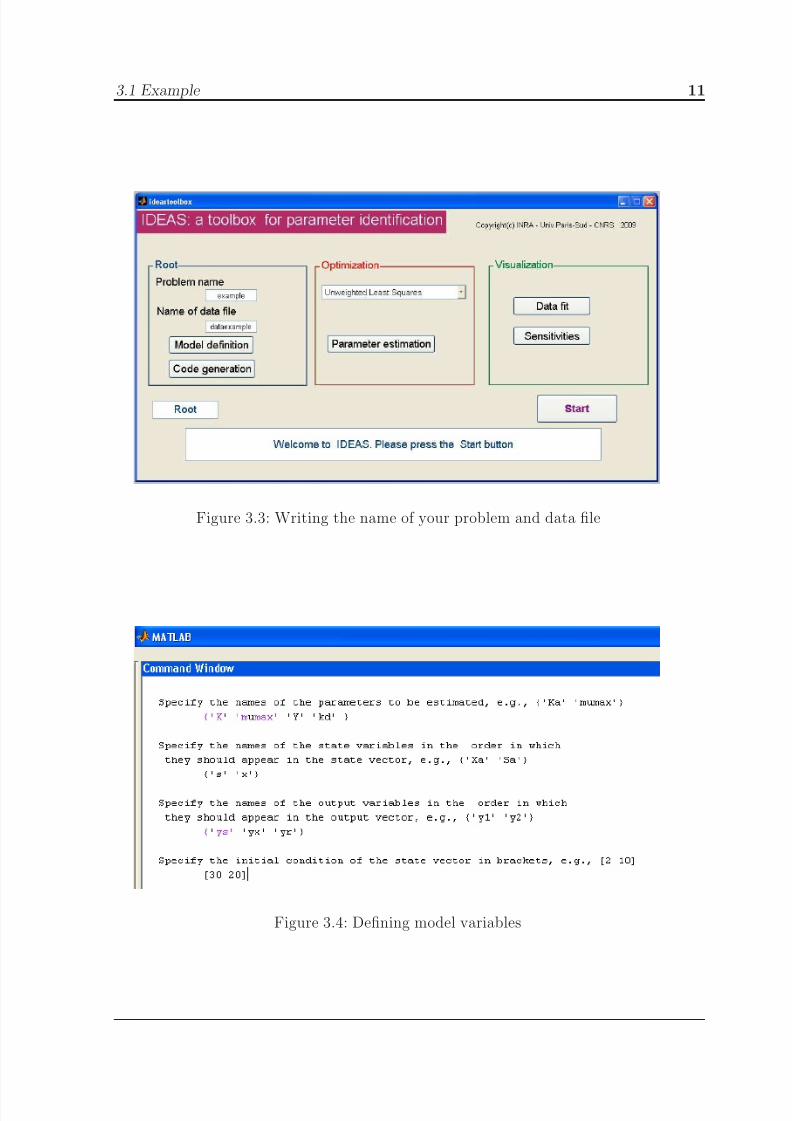
3. Follow the instructions given in the dialog box. For illustration we use example

as the name of the problem and the data file is named dataxample.txt. Figures

3.3 - 3.10 show a typical execution.



3.1 Example 11

Figure 3.3: Writing the name of your problem and data file

Figure 3.4: Defining model variables



3.1 Example 12

Figure 3.5: Defining the mathematical model. This file is automatically generated

and the user must specify the model according to the structure describe in the

template



3.1 Example 13

Figure 3.6: Press the Code generation button and then select the optimization

criterion

Figure 3.7: Writing initial guess of the parameter vector



3.1 Example 14

Figure 3.8: Estimation process. The user can choose to export the results in .xls or

.txt format. The file with the resuls is named with the suffix results



3.1 Example 15

Figure 3.9: Press the Data fit button to display the match of the model against the

data



3.1 Example 16

Figure 3.10: Press the Sensitivities button to display the trajectory of the sensitiv-

ities of the output. A final figure is a matrix representation of the L1 norm of the

normalized sensitivities. The element k, j is computed asnt

i=1

θjymk

(ti, θ)∂ymk

∂θj

(ti, θ)



3.2 Some hints 17

3.2 Some hints

The optimization step can be sensitive to numerical problems. If your estima-

tion problem cannot be solved and you have as return warning messages, it

can be due to the initialization of the parameter vector or errors in the integra-

tion of the ODE equations. You can try to make a reparametrization in order

to work in log-base. You can enter to the functions with suffixes optim and

cost to uncomment the instructions to work with this base. Advantage of this

option is that the positivity of the parameters is guaranteed. Keep in mind

that optimization is local, thus you should test the estimation with different

parameter values for the initialization.



References

[1] Goodwin, G., and Payne, R. Dynamic System Identification: Experiment

Design and Data Analysis. Academic Press, New York, 1977.

[2] Munoz-Tamayo, R., Laroche, B., Leclerc, M., and Walter, E.

IDEAS: a parameter identification toolbox with symbolic analysis of uncer-

tainty and its application to biological modelling. In 15th Symposium on System

Identification (2009).

[3] Walter, E., and Pronzato, L. Identification of Parametric Models from

Experimental Data . Springer, London, 1997.

18

IDEAS_ User Guide

Documents

Transcript of IDEAS_ User Guide