ICYSB, 2013Schaber 1/42 Introduction to Modelling Signalling Cascades in Yeast Jörg Schaber...

ICYSB, 2013 Schaber 1/42

Introduction to Modelling Signalling Cascades in Yeast

Jörg Schaber

Institute for Experimental Internal Medicine

Otto-von-Guericke University

Magdeburg

www.sysbiolab.net


• The modelling process• A simple step-by-step example

– The Sho1 branch of the HOG pathway• Basic concepts

– Signalling motifs– Model selection

Outline


• Modelling requires verbal hypothesis be made specific and conceptually rigorous.

Why Models?

• Modelling highlights gaps in our knowledge.

• Modelling provides quantitative as well as qualitative predictions.

• Modelling is ideal for analysing complex interactions before experimental tests.

• Modelling is a low-cost, rapid test bed for candidate interventions.

• Well designed models are readily portable and adaptable for many purposes.


ObservationPrior knowledge

• The observation of a natural phenomena drives a scientific question, which is represented by a testable hypothesis.

• This is the most important step as it sets the stage for the rest.

• Requires intuition and talent.

• The word model is the abstract representation of the processes that might explain data based on the hypothesis.

• Often represented by a diagram.

• Defines the components and their interactions.

• Defines systems boundaries.

• The math model is the formalised word model.

• The formalism depends on the processes and data, e.g.• dynamic systems:

ODEs• gene networks:

boolean models

• The verification is a first qualitative evaluation of the model.

• Checks whether the model is in principle able to explain the data, e.g.• if the data shows

oscillations, the model should be able to oscillate as well.

• The validation is a quantitative evaluation of the model.

• Checks whether the model is able to explain the data quantitatively.

• Fitting model to the data.

• Parameter optimization

• A successful validation consolidates our trust that we have captured the most important processes to explain the data.

• This justifies an analysis of model properties, e.g.• sensitivities• robustness

• The analysis may give indications for useful predictions.

• Sensitivity analysis may suggest a parameter with high impact on certain behaviour.

• We can define the ‘most informative’ experiment.

ObservationPrior knowledge

Math ModelMath Model

Analysis

Validation

Verification

Word Model

Hypothesis

Prediction

Analysis

Validation

Verification

Word Model

Hypothesis

The Modelling Process in 8 Steps

• A successful prediction consolidates our trust in the model and the hypothesis and that we have identified the most important processes to explain the data.

• Usually a prediction is not successful.

• Often we have to change our model/hypothesis in the course of the modelling process.

• Each modelling round deepens our understanding.


A Step-by-Step Example

The Sho1-branch of the HOG pathway


Oligomer-deficient

Oligomer-deficientPhospho-mimic

Hao et al. (2007) Curr. Biol. 17

sho1D ssk1D

The Data• It was shown that

a) Sho1 de-oligomerizes upon osmotic shockb) Hog1 phosphorylates de-oligomerized Sho1c) Phosphorylated Sho1 is less able to transmit

the signal


The Hypothesis

– Phosphorylation of Sho1 by Hog1 constitutes a negative feedback loop.

– This negative feedback leads to the rapid attenuation of Hog1 signalling.

– Might be important to dampen crosstalk to pheromone signalling pathway.


The Word Model(s)

• Signal: high osmolarity• Hog1 de-sensitizes Sho1



Formalising Word Models

Pbs2P

Hog1

‘Biologist’ notation

Not very useful (for modelling), becauseinteractions not clear.

Pbs2P

Hog1P

‘Systems Biologist’ notation

Hog1v1

v2

More useful, because each interaction is made specific.This facilitates mathematical formulation.



Pbs2P

Hog1PHog1v1

v2

• arrows between components indicate transformations, i.e. biochemical reactions, mass flows. They determine changes in concentrations, numbers, etc.

• Instead of giving explicit formulas for components, e.g. HogP(t)=f(v1,v2), we rather characterise the change of components over time.• Change = what goes in

– what goes out



Pbs2P

Hog1PHog1v1

v2

• That is one reason, why ordinary differential equation (ODE) models are so popular: easy to set up given a carefully set up wiring scheme:

21

21

1

1

vvdt

dHog

vvdt

PdHog

Note that Pbs2P does not change.



Pbs2P

Hog1PHog1v1

v2

• arrows on arrows indicate modifying interactions (enzymatic reactions), i.e. no (net) mass flows or concentrations changes involved from emanating components.

Biochemical notation

Hog1 + Pbs2P -> Hog1P + Pbs2P

Pbs2P neither consumed nor produced (netto-wise)



Pbs2P

Hog1PHog1v1

v2


v1: Hog1 + Pbs2P -> Hog1P + Pbs2P

v2: Hog1P -> Hog1

Most simple mathematical formulation: mass action kinetics, i.e. multiplication of substrates.

v1: k1·Hog1·Pbs2Pv2: k2·Hog1P

21

21

1

1

vvdt

dHog

vvdt

PdHog



• Set up wiring scheme, where each considered reaction with modifiers is made explicit.

• Formulate ODE system with balance equations.

• Choose kinetics rate formulation.

• Choose initial conditions.

Þ Theory tells us:a) There exists a solution.b) The solution is unique.c) The solution can be arbitrarily approximated.



Fus3

Fus3-Ste5

Ste5

v1

v2


v1: Fus3 + Ste5 -> Fus3-Ste5

v2: Fus3-Ste5 -> Fus3 + Ste5

Most simple mathematical formulation: mass action kinetics, i.e. linear multiplication of substrates.

v1: k1·Fus3·Ste5v2: k2·Fus3-Ste5

21

21

21

53

5

3

vvdt

StedFus

vvdt

dSte

vvdt

dFus


Kinetic rate laws and signalling motifs

Pv1

Constant fluxand simple mass action degradation

v2

Pkkdt

dP21

P

v1

Modified constant fluxand simple mass action degradation

v2 PkSkdt

dP

Skdt

dS

2

3

1

S v3

2

2

1

10

k

kP

Pkk

2

1

k

k

0)0( tP

1)0(

0)0(

tS

tP


Pv1

Modified conversion with signal degradationMass action kinetics

v2

1

)1( 2

3

1

PQ

PkPSkdt

dP

Skdt

dSS v3

Q

Pv1

Modified conversion with signal degradationMichaelis-Menten kinetics

v2

S v3

Q

PKm

Pk

PKm

PSk

dt

dP

SKm

Sk

dt

dS

2

2

1

3

3

1

)1(1

k3

k3/2

Km3



Pv1

Modified conversion with signal degradationHill kinetics

v2

S v3

Q

22

2

2

11

1

11

33

3

3

2

3

)1(

)1(hh

h

hh

h

hh

h

PKm

Pk

PKm

PSk

dt

dP

SKm

Sk

dt

dS

k3/2

Km3

k3



Pv1

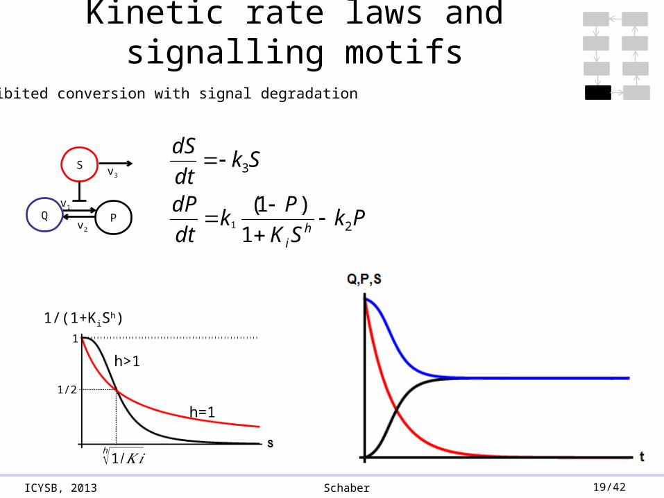
Inhibited conversion with signal degradation

v2

S v3

Q PkSK

Pk

dt

dP

Skdt

dS

hi

2

3

1

)1(1


1/2

h√1/𝐾 𝑖

1

1/(1+KiSh)

h=1

h>1


P

v1

Modified conversion with negative feedback

v2

S

Q

PkPK

PSk

dt

dPh

i21

)1(1

Observation:• System reaches new

steady state.• No ‘overshoot’

Possible explanation:• Feedback comes too

fast.



P

v1

Modified conversion with delayed negative feedback

v2

S

Q

PktPK

PSk

dt

dPh

i2)(1

)1(1

Observation:

• System ‘overshoots’, but still reaches new steady state.

• damped oscillations• The feedback to P

depends directly from P itself -> ‘auto-inhibitory feedback’



Modified conversion with negative feedback

Let’s do the math: Calculate steady-states of P(S) of a simplified system(all constants = 1)

PP

PS

dt

dP

1

)1(

261S-1-2

11

)1(0

SSP

PP

PS

In the steady-state:

Our analysis suggests that in a system with auto-inhibitory negative feedback, the steady-state depends on the input signal.


The Mathematical Model

• Signal: high osmolarity• Hog1 de-sensitizes Sho1• Delayed auto-inhibitory

feedback• Michaelis-Menten kinetics (20

parameters)• Model was fitted to Hog1

activation data



Validation

Orig. 1 M KCl

Orig. 0.5 M KClOrig. 0.25 M KCl

Single shock Double shock

- Model fits data well. - Simulations show damped oscillations and increasing

steady states- possible spurious effects due to over-parameterization


Predictions

Orig. P-Hog1

Orig. Sho1aOrig. Sho1i

0.4 M KCl tripple shock (0, 30, 60 min)


Conclusion after first modelling round

• Auto-inhibitory feedback model fits single and double shock data well, but• shows increasing steady states with increasing

external osmolarity (not supported by data),• shows damped oscillations (not supported by data, but

might be due to over-parameterization)• Auto-inhibitory feedback model is not able to predict triple

shock experiment, because of desensitization.

Possible solution: a) the signal has to be removed by adaptation b) no desensitization


Recalling the biology

Sln1Sho1

Pbs2

Hog1

P

P

Fps1

Glycerol

Hog1 P

Gpd1

Sln1Sho1

Hog1 P

• Increasing the ambientosmotic pressure leads to a rapid passive loss of water and cell skrinkage

• This leads to closure of the glycerol channel and activation of two parallel signaling branches that both activate Hog1.

• Activated Hog1 translocates to the nucleous and triggers production of enzyme that enhance glycerol prodction.• Increased glycerol equilibrates

water potential differences and forces water back into the cell leading to volume adaptation and HOG pathway deactivation.


New Hypothesis

– The signal is the water potential difference (differences in osmolarity) rather than merely external osmolarity.

– The main feedback is via glycerol accumulation.


The new word model

Signal

OuterOsmolarity

Hog1 P-Hog1

Glycerol

v3v1

v2

• Signal = OuterOmolarity-Glycerol

• 3 reactions with mass actions, i.e. 3 parameters


The mathematical model

Signal

OuterOsmolarity

Hog1 P-Hog1

Glycerol

v3v1

v2

PHogkdt

dG

PHogkPHogGOkdt

PdHog

1

1)11)((1

3

21

– For simplicity we assume Hog1+Hog1P=1

– OuterOsmolarity (O) fixed input function.

– The feedback depends on increasing Glycerol, which stays even if Hog1P=0(𝐻𝑜𝑔1𝑃0 ,𝐺0 )=(0 ,𝑂0)


Verification of the model

PHogk

PHogkPHogGOk

10

1)11)((0

3

21

Let’s do the math: Calculate steady-states

01

PHog

GO

In the steady-state:

1. In the steady state Hog1P=0 independent from the outer osmolarity.

Þ The system tracks the ‘desired’ steady state of Hog1P=0 independent from perturbations.

Þ Integral feedback property.Þ ‘Perfect adaptor’ (in Hog1P).

2. Internal glycerol concentration depends on the outer osmolarity.


A block diagram of integral feedback control.

Yi T et al. PNAS 2000;97:4649-4653

©2000 by National Academy of Sciences

• Variable u is the input for a process with gain k.

• Difference between the actual output y1 and the steady-state, i.e. ‘desired’, output y0 represents the normalized output or error y.

• Integral control arises through the feedback loop in which the time integral of y, x, is fed back into the system.

• As a result, we have ẋ = y and y = 0 at steady-state for all u.


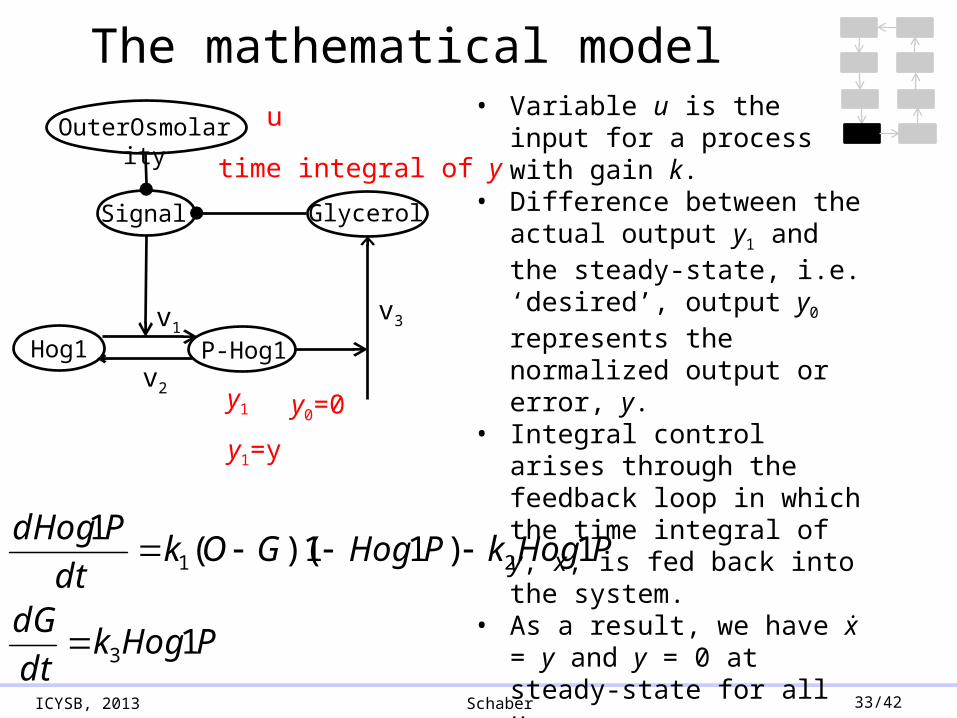
The mathematical model

Signal

OuterOsmolarity

Hog1 P-Hog1

Glycerol

v3v1

v2

PHogkdt

dG

PHogkPHogGOkdt

PdHog

1

1)11)((1

3

21

• Variable u is the input for a process with gain k.

• Difference between the actual output y1 and the steady-state, i.e. ‘desired’, output y0 represents the normalized output or error, y.

• Integral control arises through the feedback loop in which the time integral of y, x, is fed back into the system.

• As a result, we have ẋ = y and y = 0 at steady-state for all u.

u

y1 y0=0

time integral of y

y1=y


Validation of the model

Single shock

- Simulations show reasonable fits and perfect adaptation

Double shock

1 M KCl

0.5 M KCl0.25 M KCl


Prediction

- Simple model reacts to triple shock and shows perfect adaptation.

P-Hog1l

InnerOsmolarityOuterOsmolarity

0.4 M KCl tripple shock (0, 30, 60 min)


RemarksIntegral Feedback (3 parameters) Auto-inhibitory feedback (20 parameters)

• From the quality of the fit, the auto-inhibitory feedback model is much better than the integral feedback model.

• The quality of the fit is usually measured by the sum of squared residuals.

1 M KCl

0.5 M KCl0.25 M KCl

• If it weren’t for the prediction, which model is better?

n

ii

n

iii rptfyypSSR

1

2

1

2),((),(

r1

r2

r3


RemarksIntegral Feedback (3 parameters) Transient feedback (20 parameters)

• Intuitively: both model capture the basic features of the data.

• In other words: The main information in the data is reproduced by the models.

• But: the information/parameter is much higher in the simpler model.

=> The parameters of the simpler model are more informative.

1 M KCl

0.5 M KCl0.25 M KCl


The principle of parsimony• If we take the number of parameters as a measure for structural

properties of the data, we want to have few parameters, i.e. the most important structural features, and a good data representation.

“Everything should be madeas simple as possible, but not simpler.”

• Parsimony can be measured by the Akaike Information Criterion (AIC). nSSRnkAIC log2

• the lower AIC, the better the model approximates the data in terms of parsimony (k number of parameters, n number of data).

• We do not want to have additional parameter to ‘fit the errors’ or spurious effects.

• The simpler the model, the easier to analyse.

• Therefore, it is advisable to have a model that is as simple as possible and as complex as necessary: this is the principle of parsimony.


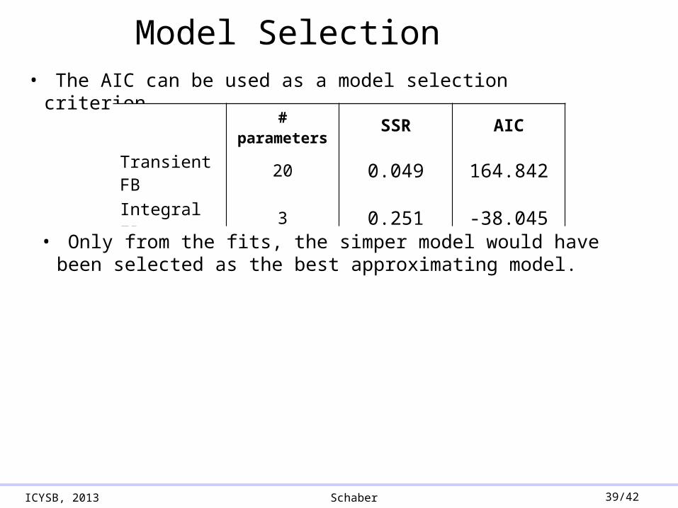
Model Selection• The AIC can be used as a model selection criterion

# parameters SSR AIC

Transient FB 20 0.049 164.842

Integral FB 3 0.251 -38.045

• Only from the fits, the simper model would have been selected as the best approximating model.


Conclusions concerning feedback in Sho1-branch

• According to the AIC, the data does not support a model with auto-inhibitory feedback, but rather a model with integral feedback.

• Therefore, for the adaptation and attenuation process, the proposed feedback of Hog1 on Sho1 is not necessary.

• The proposed feedback of Hog1 to Sho1 may modulate the signal and serve other purposes (crosstalk, stabilisation), but cannot explain adaptation to single and multiple shock.


Final Remarks on Sho1-Modelling

• The integral feedback model has several shortcoming:

• glycerol is only accumulated, never lost.Þ Adaptation to a lowering in external osmolarity cannot be

modelled

• initial Hog1P is zero

All models are wrong, but some are useful.

• Our model was developed to address the question, whether or not the (multiple) osmotic shock data can be explained by a transient feedback, nothing else.

• All models are tailored to address specific questions. No model can explain everything.

• The clearer our hypotheses are formulated, the better models can be developed to address these.


Final Remarks on Modelling

• The ‘truth’ (full reality) in biological sciences has infinite complexity and, hence, can never be revealed with only finite samples and a ‘model’ of those data.

• It is a mistake to believe that there is a simple “true model” and that during data analysis this model can be uncovered and its parameters estimated.

• We can only hope to identify a model that provides a good approximation to the data available.

• Uncertainty about the biology leads to multiple hypotheses about the underlying processes explaining a set of data.

• I recommend the formulation of multiple working hypotheses, and the building of a small set of models to clearly and uniquely represent these hypotheses.

• The best approximating model can then be identified by model selection criteria.

ICYSB, 2013Schaber 1/42 Introduction to Modelling Signalling Cascades in Yeast Jörg Schaber...

Documents

Transcript of ICYSB, 2013Schaber 1/42 Introduction to Modelling Signalling Cascades in Yeast Jörg Schaber...