IBM SPSS Complex Samples 22 - University of · PDF filein a data file represent a simple...
64
IBM SPSS Complex Samples 22
Transcript of IBM SPSS Complex Samples 22 - University of · PDF filein a data file represent a simple...
IBM SPSS Complex Samples 22
���

NoteBefore using this information and the product it supports, read the information in “Notices” on page 51.
Product Information
This edition applies to version 22, release 0, modification 0 of IBM SPSS Statistics and to all subsequent releases andmodifications until otherwise indicated in new editions.

Contents
Chapter 1. Introduction to ComplexSamples Procedures . . . . . . . . . 1Properties of Complex Samples . . . . . . . . 1Usage of Complex Samples Procedures . . . . . 2
Plan Files . . . . . . . . . . . . . . 2Further Readings . . . . . . . . . . . . . 2
Chapter 2. Sampling from a ComplexDesign . . . . . . . . . . . . . . . 3Creating a New Sample Plan . . . . . . . . . 3Sampling Wizard: Design Variables . . . . . . . 3
Tree Controls for Navigating the Sampling Wizard 4Sampling Wizard: Sampling Method . . . . . . 4Sampling Wizard: Sample Size . . . . . . . . 5
Define Unequal Sizes . . . . . . . . . . 5Sampling Wizard: Output Variables. . . . . . . 5Sampling Wizard: Plan Summary . . . . . . . 6Sampling Wizard: Draw Sample Selection Options. . 6Sampling Wizard: Draw Sample Output Files . . . 6Sampling Wizard: Finish . . . . . . . . . . 7Modifying an Existing Sample Plan. . . . . . . 7Sampling Wizard: Plan Summary . . . . . . . 7Running an Existing Sample Plan . . . . . . . 8CSPLAN and CSSELECT Commands AdditionalFeatures . . . . . . . . . . . . . . . . 8
Chapter 3. Preparing a Complex Samplefor Analysis . . . . . . . . . . . . . 9Creating a New Analysis Plan . . . . . . . . 9Analysis Preparation Wizard: Design Variables . . . 9
Tree Controls for Navigating the Analysis Wizard 10Analysis Preparation Wizard: Estimation Method . . 10Analysis Preparation Wizard: Size . . . . . . . 10
Define Unequal Sizes . . . . . . . . . . 11Analysis Preparation Wizard: Plan Summary . . . 11Analysis Preparation Wizard: Finish . . . . . . 11Modifying an Existing Analysis Plan . . . . . . 12Analysis Preparation Wizard: Plan Summary . . . 12
Chapter 4. Complex Samples Plan . . . 13
Chapter 5. Complex SamplesFrequencies . . . . . . . . . . . . 15Complex Samples Frequencies Statistics . . . . . 15Complex Samples Missing Values . . . . . . . 16Complex Samples Options . . . . . . . . . 16
Chapter 6. Complex SamplesDescriptives . . . . . . . . . . . . 17Complex Samples Descriptives Statistics . . . . . 17Complex Samples Descriptives Missing Values . . 18Complex Samples Options . . . . . . . . . 18
Chapter 7. Complex SamplesCrosstabs . . . . . . . . . . . . . 19Complex Samples Crosstabs Statistics. . . . . . 19Complex Samples Missing Values . . . . . . . 20Complex Samples Options . . . . . . . . . 21
Chapter 8. Complex Samples Ratios . . 23Complex Samples Ratios Statistics . . . . . . . 23Complex Samples Ratios Missing Values . . . . 23Complex Samples Options . . . . . . . . . 24
Chapter 9. Complex Samples GeneralLinear Model . . . . . . . . . . . . 25Complex Samples General Linear Model . . . . 25Complex Samples General Linear Model Statistics 26Complex Samples Hypothesis Tests . . . . . . 27Complex Samples General Linear Model EstimatedMeans . . . . . . . . . . . . . . . . 27Complex Samples General Linear Model Save . . . 28Complex Samples General Linear Model Options. . 28CSGLM Command Additional Features . . . . . 28
Chapter 10. Complex Samples LogisticRegression . . . . . . . . . . . . . 29Complex Samples Logistic Regression ReferenceCategory . . . . . . . . . . . . . . . 29Complex Samples Logistic Regression Model . . . 29Complex Samples Logistic Regression Statistics . . 30Complex Samples Hypothesis Tests . . . . . . 31Complex Samples Logistic Regression Odds Ratios 31Complex Samples Logistic Regression Save . . . . 32Complex Samples Logistic Regression Options . . 32CSLOGISTIC Command Additional Features . . . 33
Chapter 11. Complex Samples OrdinalRegression . . . . . . . . . . . . . 35Complex Samples Ordinal Regression ResponseProbabilities . . . . . . . . . . . . . . 35Complex Samples Ordinal Regression Model . . . 36Complex Samples Ordinal Regression Statistics . . 36Complex Samples Hypothesis Tests . . . . . . 37Complex Samples Ordinal Regression Odds Ratios 38Complex Samples Ordinal Regression Save . . . . 38Complex Samples Ordinal Regression Options. . . 39CSORDINAL Command Additional Features . . . 39
Chapter 12. Complex Samples CoxRegression . . . . . . . . . . . . . 41Define Event . . . . . . . . . . . . . . 42Predictors . . . . . . . . . . . . . . . 42
Define Time-Dependent Predictor . . . . . . 43Subgroups . . . . . . . . . . . . . . . 43Model . . . . . . . . . . . . . . . . 43
iii

Statistics . . . . . . . . . . . . . . . 44Plots. . . . . . . . . . . . . . . . . 45Hypothesis Tests. . . . . . . . . . . . . 45Save . . . . . . . . . . . . . . . . . 46Export . . . . . . . . . . . . . . . . 47Options. . . . . . . . . . . . . . . . 48CSCOXREG Command Additional Features . . . 48
Notices . . . . . . . . . . . . . . 51Trademarks . . . . . . . . . . . . . . 53
Index . . . . . . . . . . . . . . . 55
iv IBM SPSS Complex Samples 22
Chapter 1. Introduction to Complex Samples Procedures
An inherent assumption of analytical procedures in traditional software packages is that the observationsin a data file represent a simple random sample from the population of interest. This assumption isuntenable for an increasing number of companies and researchers who find it both cost-effective andconvenient to obtain samples in a more structured way.
The Complex Samples option allows you to select a sample according to a complex design andincorporate the design specifications into the data analysis, thus ensuring that your results are valid.
Properties of Complex SamplesA complex sample can differ from a simple random sample in many ways. In a simple random sample,individual sampling units are selected at random with equal probability and without replacement (WOR)directly from the entire population. By contrast, a given complex sample can have some or all of thefollowing features:
Stratification. Stratified sampling involves selecting samples independently within non-overlappingsubgroups of the population, or strata. For example, strata may be socioeconomic groups, job categories,age groups, or ethnic groups. With stratification, you can ensure adequate sample sizes for subgroups ofinterest, improve the precision of overall estimates, and use different sampling methods from stratum tostratum.
Clustering. Cluster sampling involves the selection of groups of sampling units, or clusters. For example,clusters may be schools, hospitals, or geographical areas, and sampling units may be students, patients,or citizens. Clustering is common in multistage designs and area (geographic) samples.
Multiple stages. In multistage sampling, you select a first-stage sample based on clusters. Then youcreate a second-stage sample by drawing subsamples from the selected clusters. If the second-stagesample is based on subclusters, you can then add a third stage to the sample. For example, in the firststage of a survey, a sample of cities could be drawn. Then, from the selected cities, households could besampled. Finally, from the selected households, individuals could be polled. The Sampling and AnalysisPreparation wizards allow you to specify three stages in a design.
Nonrandom sampling. When selection at random is difficult to obtain, units can be sampledsystematically (at a fixed interval) or sequentially.
Unequal selection probabilities. When sampling clusters that contain unequal numbers of units, you canuse probability-proportional-to-size (PPS) sampling to make a cluster's selection probability equal to theproportion of units it contains. PPS sampling can also use more general weighting schemes to selectunits.
Unrestricted sampling. Unrestricted sampling selects units with replacement (WR). Thus, an individualunit can be selected for the sample more than once.
Sampling weights. Sampling weights are automatically computed while drawing a complex sample andideally correspond to the "frequency" that each sampling unit represents in the target population.Therefore, the sum of the weights over the sample should estimate the population size. Complex Samplesanalysis procedures require sampling weights in order to properly analyze a complex sample. Note thatthese weights should be used entirely within the Complex Samples option and should not be used withother analytical procedures via the Weight Cases procedure, which treats weights as case replications.
© Copyright IBM Corporation 1989, 2013 1

Usage of Complex Samples ProceduresYour usage of Complex Samples procedures depends on your particular needs. The primary types ofusers are those who:v Plan and carry out surveys according to complex designs, possibly analyzing the sample later. The
primary tool for surveyors is the Sampling Wizard.v Analyze sample data files previously obtained according to complex designs. Before using the Complex
Samples analysis procedures, you may need to use the Analysis Preparation Wizard.
Regardless of which type of user you are, you need to supply design information to Complex Samplesprocedures. This information is stored in a plan file for easy reuse.
Plan FilesA plan file contains complex sample specifications. There are two types of plan files:
Sampling plan. The specifications given in the Sampling Wizard define a sample design that is used todraw a complex sample. The sampling plan file contains those specifications. The sampling plan file alsocontains a default analysis plan that uses estimation methods suitable for the specified sample design.
Analysis plan. This plan file contains information needed by Complex Samples analysis procedures toproperly compute variance estimates for a complex sample. The plan includes the sample structure,estimation methods for each stage, and references to required variables, such as sample weights. TheAnalysis Preparation Wizard allows you to create and edit analysis plans.
There are several advantages to saving your specifications in a plan file, including:v A surveyor can specify the first stage of a multistage sampling plan and draw first-stage units now,
collect information on sampling units for the second stage, and then modify the sampling plan toinclude the second stage.
v An analyst who doesn't have access to the sampling plan file can specify an analysis plan and refer tothat plan from each Complex Samples analysis procedure.
v A designer of large-scale public use samples can publish the sampling plan file, which simplifies theinstructions for analysts and avoids the need for each analyst to specify his or her own analysis plans.
Further ReadingsFor more information on sampling techniques, see the following texts:
Cochran, W. G. 1977. Sampling Techniques, 3rd ed. New York: John Wiley and Sons.
Kish, L. 1965. Survey Sampling. New York: John Wiley and Sons.
Kish, L. 1987. Statistical Design for Research. New York: John Wiley and Sons.
Murthy, M. N. 1967. Sampling Theory and Methods. Calcutta, India: Statistical Publishing Society.
Särndal, C., B. Swensson, and J. Wretman. 1992. Model Assisted Survey Sampling. New York:Springer-Verlag.
2 IBM SPSS Complex Samples 22

Chapter 2. Sampling from a Complex Design
The Sampling Wizard guides you through the steps for creating, modifying, or executing a sampling planfile. Before using the Wizard, you should have a well-defined target population, a list of sampling units,and an appropriate sample design in mind.
Creating a New Sample Plan1. From the menus choose:
Analyze > Complex Samples > Select a Sample...
2. Select Design a sample and choose a plan filename to save the sample plan.3. Click Next to continue through the Wizard.4. Optionally, in the Design Variables step, you can define strata, clusters, and input sample weights.
After you define these, click Next.5. Optionally, in the Sampling Method step, you can choose a method for selecting items.
If you select PPS Brewer or PPS Murthy, you can click Finish to draw the sample. Otherwise, clickNext and then:
6. In the Sample Size step, specify the number or proportion of units to sample.7. You can now click Finish to draw the sample.
Optionally, in further steps you can:v Choose output variables to save.v Add a second or third stage to the design.v Set various selection options, including which stages to draw samples from, the random number seed,
and whether to treat user-missing values as valid values of design variables.v Choose where to save output data.v Paste your selections as command syntax.
Sampling Wizard: Design VariablesThis step allows you to select stratification and clustering variables and to define input sample weights.You can also specify a label for the stage.
Stratify By. The cross-classification of stratification variables defines distinct subpopulations, or strata.Separate samples are obtained for each stratum. To improve the precision of your estimates, units withinstrata should be as homogeneous as possible for the characteristics of interest.
Clusters. Cluster variables define groups of observational units, or clusters. Clusters are useful whendirectly sampling observational units from the population is expensive or impossible; instead, you cansample clusters from the population and then sample observational units from the selected clusters.However, the use of clusters can introduce correlations among sampling units, resulting in a loss ofprecision. To minimize this effect, units within clusters should be as heterogeneous as possible for thecharacteristics of interest. You must define at least one cluster variable in order to plan a multistagedesign. Clusters are also necessary in the use of several different sampling methods. See the topic“Sampling Wizard: Sampling Method” on page 4 for more information.
Input Sample Weight. If the current sample design is part of a larger sample design, you may havesample weights from a previous stage of the larger design. You can specify a numeric variable containingthese weights in the first stage of the current design. Sample weights are computed automatically forsubsequent stages of the current design.
© Copyright IBM Corporation 1989, 2013 3

Stage Label. You can specify an optional string label for each stage. This is used in the output to helpidentify stagewise information.
Note: The source variable list has the same content across steps of the Wizard. In other words, variablesremoved from the source list in a particular step are removed from the list in all steps. Variables returnedto the source list appear in the list in all steps.
Tree Controls for Navigating the Sampling WizardOn the left side of each step in the Sampling Wizard is an outline of all the steps. You can navigate theWizard by clicking on the name of an enabled step in the outline. Steps are enabled as long as allprevious steps are valid—that is, if each previous step has been given the minimum requiredspecifications for that step. See the Help for individual steps for more information on why a given stepmay be invalid.
Sampling Wizard: Sampling MethodThis step allows you to specify how to select cases from the active dataset.
Method. Controls in this group are used to choose a selection method. Some sampling types allow you tochoose whether to sample with replacement (WR) or without replacement (WOR). See the typedescriptions for more information. Note that some probability-proportional-to-size (PPS) types areavailable only when clusters have been defined and that all PPS types are available only in the first stageof a design. Moreover, WR methods are available only in the last stage of a design.v Simple Random Sampling. Units are selected with equal probability. They can be selected with or
without replacement.v Simple Systematic. Units are selected at a fixed interval throughout the sampling frame (or strata, if
they have been specified) and extracted without replacement. A randomly selected unit within the firstinterval is chosen as the starting point.
v Simple Sequential. Units are selected sequentially with equal probability and without replacement.v PPS. This is a first-stage method that selects units at random with probability proportional to size. Any
units can be selected with replacement; only clusters can be sampled without replacement.v PPS Systematic. This is a first-stage method that systematically selects units with probability
proportional to size. They are selected without replacement.v PPS Sequential. This is a first-stage method that sequentially selects units with probability
proportional to cluster size and without replacement.v PPS Brewer. This is a first-stage method that selects two clusters from each stratum with probability
proportional to cluster size and without replacement. A cluster variable must be specified to use thismethod.
v PPS Murthy. This is a first-stage method that selects two clusters from each stratum with probabilityproportional to cluster size and without replacement. A cluster variable must be specified to use thismethod.
v PPS Sampford. This is a first-stage method that selects more than two clusters from each stratum withprobability proportional to cluster size and without replacement. It is an extension of Brewer's method.A cluster variable must be specified to use this method.
v Use WR estimation for analysis. By default, an estimation method is specified in the plan file that isconsistent with the selected sampling method. This allows you to use with-replacement estimationeven if the sampling method implies WOR estimation. This option is available only in stage 1.
Measure of Size (MOS). If a PPS method is selected, you must specify a measure of size that defines thesize of each unit. These sizes can be explicitly defined in a variable or they can be computed from thedata. Optionally, you can set lower and upper bounds on the MOS, overriding any values found in theMOS variable or computed from the data. These options are available only in stage 1.
4 IBM SPSS Complex Samples 22
Sampling Wizard: Sample SizeThis step allows you to specify the number or proportion of units to sample within the current stage. Thesample size can be fixed or it can vary across strata. For the purpose of specifying sample size, clusterschosen in previous stages can be used to define strata.
Units. You can specify an exact sample size or a proportion of units to sample.v Value. A single value is applied to all strata. If Counts is selected as the unit metric, you should enter
a positive integer. If Proportions is selected, you should enter a non-negative value. Unless samplingwith replacement, proportion values should also be no greater than 1.
v Unequal values for strata. Allows you to enter size values on a per-stratum basis via the DefineUnequal Sizes dialog box.
v Read values from variable. Allows you to select a numeric variable that contains size values for strata.
If Proportions is selected, you have the option to set lower and upper bounds on the number of unitssampled.
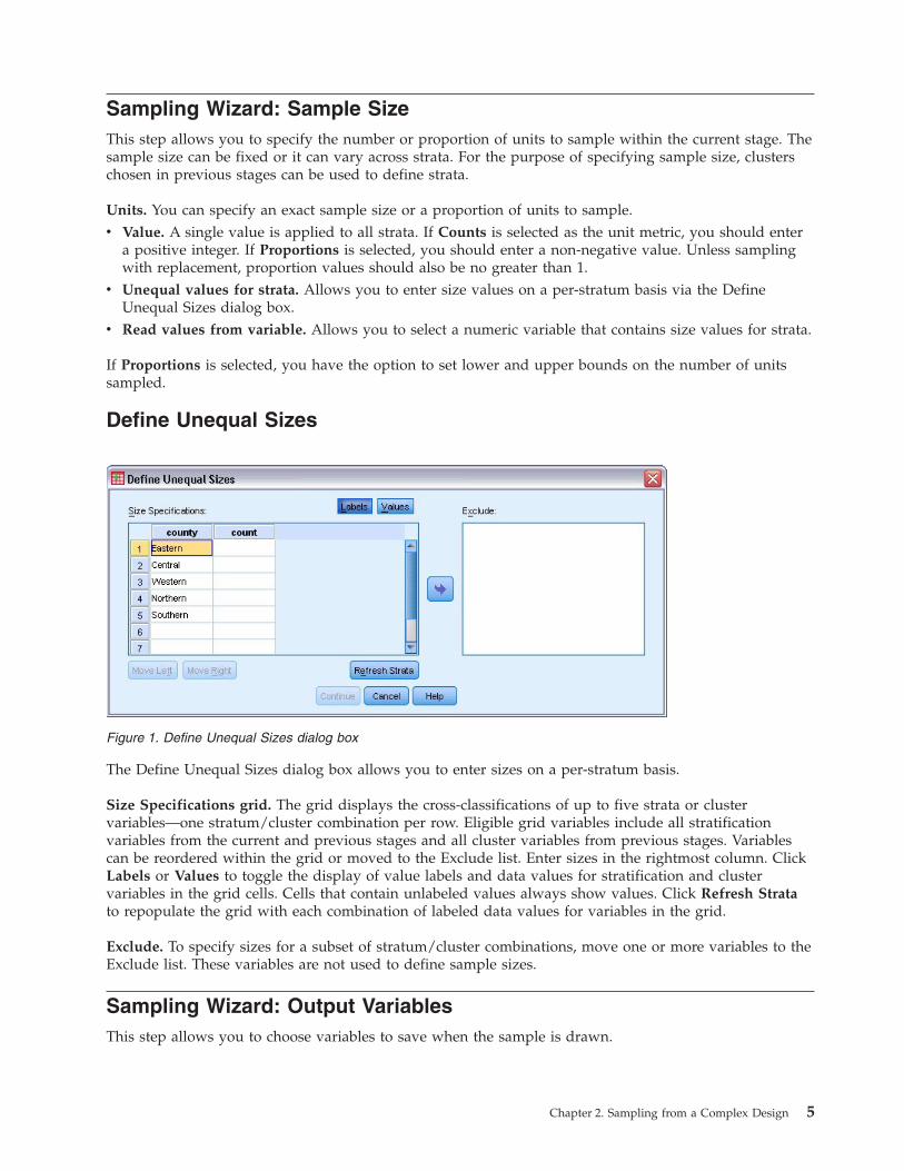
Define Unequal Sizes
The Define Unequal Sizes dialog box allows you to enter sizes on a per-stratum basis.
Size Specifications grid. The grid displays the cross-classifications of up to five strata or clustervariables—one stratum/cluster combination per row. Eligible grid variables include all stratificationvariables from the current and previous stages and all cluster variables from previous stages. Variablescan be reordered within the grid or moved to the Exclude list. Enter sizes in the rightmost column. ClickLabels or Values to toggle the display of value labels and data values for stratification and clustervariables in the grid cells. Cells that contain unlabeled values always show values. Click Refresh Stratato repopulate the grid with each combination of labeled data values for variables in the grid.
Exclude. To specify sizes for a subset of stratum/cluster combinations, move one or more variables to theExclude list. These variables are not used to define sample sizes.
Sampling Wizard: Output VariablesThis step allows you to choose variables to save when the sample is drawn.
Figure 1. Define Unequal Sizes dialog box
Chapter 2. Sampling from a Complex Design 5
Population size. The estimated number of units in the population for a given stage. The rootname for thesaved variable is PopulationSize_.
Sample proportion. The sampling rate at a given stage. The rootname for the saved variable isSamplingRate_.
Sample size. The number of units drawn at a given stage. The rootname for the saved variable isSampleSize_.
Sample weight. The inverse of the inclusion probabilities. The rootname for the saved variable isSampleWeight_.
Some stagewise variables are generated automatically. These include:
Inclusion probabilities. The proportion of units drawn at a given stage. The rootname for the savedvariable is InclusionProbability_.
Cumulative weight. The cumulative sample weight over stages previous to and including the currentone. The rootname for the saved variable is SampleWeightCumulative_.
Index. Identifies units selected multiple times within a given stage. The rootname for the saved variableis Index_.
Note: Saved variable rootnames include an integer suffix that reflects the stage number—for example,PopulationSize_1_ for the saved population size for stage 1.
Sampling Wizard: Plan SummaryThis is the last step within each stage, providing a summary of the sample design specifications throughthe current stage. From here, you can either proceed to the next stage (creating it, if necessary) or setoptions for drawing the sample.
Sampling Wizard: Draw Sample Selection OptionsThis step allows you to choose whether to draw a sample. You can also control other sampling options,such as the random seed and missing-value handling.
Draw sample. In addition to choosing whether to draw a sample, you can also choose to execute part ofthe sampling design. Stages must be drawn in order—that is, stage 2 cannot be drawn unless stage 1 isalso drawn. When editing or executing a plan, you cannot resample locked stages.
Seed. This allows you to choose a seed value for random number generation.
Include user-missing values. This determines whether user-missing values are valid. If so, user-missingvalues are treated as a separate category.
Data already sorted. If your sample frame is presorted by the values of the stratification variables, thisoption allows you to speed the selection process.
Sampling Wizard: Draw Sample Output FilesThis step allows you to choose where to direct sampled cases, weight variables, joint probabilities, andcase selection rules.
Sample data. These options let you determine where sample output is written. It can be added to theactive dataset, written to a new dataset, or saved to an external IBM® SPSS® Statistics data file. Datasets
6 IBM SPSS Complex Samples 22

are available during the current session but are not available in subsequent sessions unless you explicitlysave them as data files. Dataset names must adhere to variable naming rules. If an external file or newdataset is specified, the sampling output variables and variables in the active dataset for the selectedcases are written.
Joint probabilities. These options let you determine where joint probabilities are written. They are savedto an external IBM SPSS Statistics data file. Joint probabilities are produced if the PPS WOR, PPS Brewer,PPS Sampford, or PPS Murthy method is selected and WR estimation is not specified.
Case selection rules. If you are constructing your sample one stage at a time, you may want to save thecase selection rules to a text file. They are useful for constructing the subframe for subsequent stages.
Sampling Wizard: FinishThis is the final step. You can save the plan file and draw the sample now or paste your selections into asyntax window.
When making changes to stages in the existing plan file, you can save the edited plan to a new file oroverwrite the existing file. When adding stages without making changes to existing stages, the Wizardautomatically overwrites the existing plan file. If you want to save the plan to a new file, select Paste thesyntax generated by the Wizard into a syntax window and change the filename in the syntaxcommands.
Modifying an Existing Sample Plan1. From the menus choose:
Analyze > Complex Samples > Select a Sample...
2. Select Edit a sample design and choose a plan file to edit.3. Click Next to continue through the Wizard.4. Review the sampling plan in the Plan Summary step, and then click Next.
Subsequent steps are largely the same as for a new design. See the Help for individual steps for moreinformation.
5. Navigate to the Finish step, and specify a new name for the edited plan file or choose to overwritethe existing plan file.
Optionally, you can:v Specify stages that have already been sampled.v Remove stages from the plan.
Sampling Wizard: Plan SummaryThis step allows you to review the sampling plan and indicate stages that have already been sampled. Ifediting a plan, you can also remove stages from the plan.
Previously sampled stages. If an extended sampling frame is not available, you will have to execute amultistage sampling design one stage at a time. Select which stages have already been sampled from thedrop-down list. Any stages that have been executed are locked; they are not available in the DrawSample Selection Options step, and they cannot be altered when editing a plan.
Remove stages. You can remove stages 2 and 3 from a multistage design.
Chapter 2. Sampling from a Complex Design 7
Running an Existing Sample Plan1. From the menus choose:
Analyze > Complex Samples > Select a Sample...
2. Select Draw a sample and choose a plan file to run.3. Click Next to continue through the Wizard.4. Review the sampling plan in the Plan Summary step, and then click Next.5. The individual steps containing stage information are skipped when executing a sample plan. You can
now go on to the Finish step at any time.
Optionally, you can specify stages that have already been sampled.
CSPLAN and CSSELECT Commands Additional FeaturesThe command syntax language also allows you to:v Specify custom names for output variables.v Control the output in the Viewer. For example, you can suppress the stagewise summary of the plan
that is displayed if a sample is designed or modified, suppress the summary of the distribution ofsampled cases by strata that is shown if the sample design is executed, and request a case processingsummary.
v Choose a subset of variables in the active dataset to write to an external sample file or to a differentdataset.
See the Command Syntax Reference for complete syntax information.
8 IBM SPSS Complex Samples 22
Chapter 3. Preparing a Complex Sample for Analysis
The Analysis Preparation Wizard guides you through the steps for creating or modifying an analysis planfor use with the various Complex Samples analysis procedures. Before using the Wizard, you shouldhave a sample drawn according to a complex design.
Creating a new plan is most useful when you do not have access to the sampling plan file used to drawthe sample (recall that the sampling plan contains a default analysis plan). If you do have access to thesampling plan file used to draw the sample, you can use the default analysis plan contained in thesampling plan file or override the default analysis specifications and save your changes to a new file.
Creating a New Analysis Plan1. From the menus choose:
Analyze > Complex Samples > Prepare for Analysis...
2. Select Create a plan file, and choose a plan filename to which you will save the analysis plan.3. Click Next to continue through the Wizard.4. Specify the variable containing sample weights in the Design Variables step, optionally defining strata
and clusters.5. You can now click Finish to save the plan.
Optionally, in further steps you can:v Select the method for estimating standard errors in the Estimation Method step.v Specify the number of units sampled or the inclusion probability per unit in the Size step.v Add a second or third stage to the design.v Paste your selections as command syntax.
Analysis Preparation Wizard: Design VariablesThis step allows you to identify the stratification and clustering variables and define sample weights. Youcan also provide a label for the stage.
Strata. The cross-classification of stratification variables defines distinct subpopulations, or strata. Yourtotal sample represents the combination of independent samples from each stratum.
Clusters. Cluster variables define groups of observational units, or clusters. Samples drawn in multiplestages select clusters in the earlier stages and then subsample units from the selected clusters. Whenanalyzing a data file obtained by sampling clusters with replacement, you should include the duplicationindex as a cluster variable.
Sample Weight. You must provide sample weights in the first stage. Sample weights are computedautomatically for subsequent stages of the current design.
Stage Label. You can specify an optional string label for each stage. This is used in the output to helpidentify stagewise information.
Note: The source variable list has the same contents across steps of the Wizard. In other words, variablesremoved from the source list in a particular step are removed from the list in all steps. Variables returnedto the source list show up in all steps.
© Copyright IBM Corporation 1989, 2013 9

Tree Controls for Navigating the Analysis WizardAt the left side of each step of the Analysis Wizard is an outline of all the steps. You can navigate theWizard by clicking on the name of an enabled step in the outline. Steps are enabled as long as allprevious steps are valid—that is, as long as each previous step has been given the minimum requiredspecifications for that step. For more information on why a given step may be invalid, see the Help forindividual steps.
Analysis Preparation Wizard: Estimation MethodThis step allows you to specify an estimation method for the stage.
WR (sampling with replacement). WR estimation does not include a correction for sampling from afinite population (FPC) when estimating the variance under the complex sampling design. You canchoose to include or exclude the FPC when estimating the variance under simple random sampling (SRS).
Choosing not to include the FPC for SRS variance estimation is recommended when the analysis weightshave been scaled so that they do not add up to the population size. The SRS variance estimate is used incomputing statistics like the design effect. WR estimation can be specified only in the final stage of adesign; the Wizard will not allow you to add another stage if you select WR estimation.
Equal WOR (equal probability sampling without replacement). Equal WOR estimation includes thefinite population correction and assumes that units are sampled with equal probability. Equal WOR canbe specified in any stage of a design.
Unequal WOR (unequal probability sampling without replacement). In addition to using the finitepopulation correction, Unequal WOR accounts for sampling units (usually clusters) selected with unequalprobability. This estimation method is available only in the first stage.
Analysis Preparation Wizard: SizeThis step is used to specify inclusion probabilities or population sizes for the current stage. Sizes can befixed or can vary across strata. For the purpose of specifying sizes, clusters specified in previous stagescan be used to define strata. Note that this step is necessary only when Equal WOR is chosen as theEstimation Method.
Units. You can specify exact population sizes or the probabilities with which units were sampled.v Value. A single value is applied to all strata. If Population Sizes is selected as the unit metric, you
should enter a non-negative integer. If Inclusion Probabilities is selected, you should enter a valuebetween 0 and 1, inclusive.
v Unequal values for strata. Allows you to enter size values on a per-stratum basis via the DefineUnequal Sizes dialog box.
v Read values from variable. Allows you to select a numeric variable that contains size values for strata.
10 IBM SPSS Complex Samples 22

Define Unequal Sizes
The Define Unequal Sizes dialog box allows you to enter sizes on a per-stratum basis.
Size Specifications grid. The grid displays the cross-classifications of up to five strata or clustervariables—one stratum/cluster combination per row. Eligible grid variables include all stratificationvariables from the current and previous stages and all cluster variables from previous stages. Variablescan be reordered within the grid or moved to the Exclude list. Enter sizes in the rightmost column. ClickLabels or Values to toggle the display of value labels and data values for stratification and clustervariables in the grid cells. Cells that contain unlabeled values always show values. Click Refresh Stratato repopulate the grid with each combination of labeled data values for variables in the grid.
Exclude. To specify sizes for a subset of stratum/cluster combinations, move one or more variables to theExclude list. These variables are not used to define sample sizes.
Analysis Preparation Wizard: Plan SummaryThis is the last step within each stage, providing a summary of the analysis design specifications throughthe current stage. From here, you can either proceed to the next stage (creating it if necessary) or save theanalysis specifications.
If you cannot add another stage, it is likely because:v No cluster variable was specified in the Design Variables step.v You selected WR estimation in the Estimation Method step.v This is the third stage of the analysis, and the Wizard supports a maximum of three stages.
Analysis Preparation Wizard: FinishThis is the final step. You can save the plan file now or paste your selections to a syntax window.
When making changes to stages in the existing plan file, you can save the edited plan to a new file oroverwrite the existing file. When adding stages without making changes to existing stages, the Wizardautomatically overwrites the existing plan file. If you want to save the plan to a new file, choose to Pastethe syntax generated by the Wizard into a syntax window and change the filename in the syntaxcommands.
Figure 2. Define Unequal Sizes dialog box
Chapter 3. Preparing a Complex Sample for Analysis 11
Modifying an Existing Analysis Plan1. From the menus choose:
Analyze > Complex Samples > Prepare for Analysis...
2. Select Edit a plan file, and choose a plan filename to which you will save the analysis plan.3. Click Next to continue through the Wizard.4. Review the analysis plan in the Plan Summary step, and then click Next.
Subsequent steps are largely the same as for a new design. For more information, see the Help forindividual steps.
5. Navigate to the Finish step, and specify a new name for the edited plan file, or choose to overwritethe existing plan file.
Optionally, you can remove stages from the plan.
Analysis Preparation Wizard: Plan SummaryThis step allows you to review the analysis plan and remove stages from the plan.
Remove Stages. You can remove stages 2 and 3 from a multistage design. Since a plan must have at leastone stage, you can edit but not remove stage 1 from the design.
12 IBM SPSS Complex Samples 22

Chapter 4. Complex Samples Plan
Complex Samples analysis procedures require analysis specifications from an analysis or sample plan filein order to provide valid results.
Plan. Specify the path of an analysis or sample plan file.
Joint Probabilities. In order to use Unequal WOR estimation for clusters drawn using a PPS WORmethod, you need to specify a separate file or an open dataset containing the joint probabilities. This fileor dataset is created by the Sampling Wizard during sampling.
© Copyright IBM Corporation 1989, 2013 13

14 IBM SPSS Complex Samples 22
Chapter 5. Complex Samples Frequencies
The Complex Samples Frequencies procedure produces frequency tables for selected variables anddisplays univariate statistics. Optionally, you can request statistics by subgroups, defined by one or morecategorical variables.
Example. Using the Complex Samples Frequencies procedure, you can obtain univariate tabular statisticsfor vitamin usage among U.S. citizens, based on the results of the National Health Interview Survey(NHIS) and with an appropriate analysis plan for this public-use data.
Statistics. The procedure produces estimates of cell population sizes and table percentages, plus standarderrors, confidence intervals, coefficients of variation, design effects, square roots of design effects,cumulative values, and unweighted counts for each estimate. Additionally, chi-square and likelihood-ratiostatistics are computed for the test of equal cell proportions.
Complex Samples Frequencies Data Considerations
Data. Variables for which frequency tables are produced should be categorical. Subpopulation variablescan be string or numeric but should be categorical.
Assumptions. The cases in the data file represent a sample from a complex design that should beanalyzed according to the specifications in the file selected in the Complex Samples Plan dialog box.
Obtaining Complex Samples Frequencies1. From the menus choose:
Analyze > Complex Samples > Frequencies...
2. Select a plan file. Optionally, select a custom joint probabilities file.3. Click Continue.4. In the Complex Samples Frequencies dialog box, select at least one frequency variable.
Optionally, you can specify variables to define subpopulations. Statistics are computed separately for eachsubpopulation.
Complex Samples Frequencies StatisticsCells. This group allows you to request estimates of the cell population sizes and table percentages.
Statistics. This group produces statistics associated with the population size or table percentage.v Standard error. The standard error of the estimate.v Confidence interval. A confidence interval for the estimate, using the specified level.v Coefficient of variation. The ratio of the standard error of the estimate to the estimate.v Unweighted count. The number of units used to compute the estimate.v Design effect. The ratio of the variance of the estimate to the variance obtained by assuming that the
sample is a simple random sample. This is a measure of the effect of specifying a complex design,where values further from 1 indicate greater effects.
v Square root of design effect. This is a measure of the effect of specifying a complex design, wherevalues further from 1 indicate greater effects.
v Cumulative values. The cumulative estimate through each value of the variable.
© Copyright IBM Corporation 1989, 2013 15

Test of equal cell proportions. This produces chi-square and likelihood-ratio tests of the hypothesis thatthe categories of a variable have equal frequencies. Separate tests are performed for each variable.
Complex Samples Missing Values
Tables. This group determines which cases are used in the analysis.v Use all available data. Missing values are determined on a table-by-table basis. Thus, the cases used to
compute statistics may vary across frequency or crosstabulation tables.v Use consistent case base. Missing values are determined across all variables. Thus, the cases used to
compute statistics are consistent across tables.
Categorical Design Variables. This group determines whether user-missing values are valid or invalid.
Complex Samples Options
Subpopulation Display. You can choose to have subpopulations displayed in the same table or inseparate tables.
Figure 3. Missing Values dialog box
Figure 4. Options dialog box
16 IBM SPSS Complex Samples 22
Chapter 6. Complex Samples Descriptives
The Complex Samples Descriptives procedure displays univariate summary statistics for several variables.Optionally, you can request statistics by subgroups, defined by one or more categorical variables.
Example. Using the Complex Samples Descriptives procedure, you can obtain univariate descriptivestatistics for the activity levels of U.S. citizens, based on the results of the National Health InterviewSurvey (NHIS) and with an appropriate analysis plan for this public-use data.
Statistics. The procedure produces means and sums, plus t tests, standard errors, confidence intervals,coefficients of variation, unweighted counts, population sizes, design effects, and square roots of designeffects for each estimate.
Complex Samples Descriptives Data Considerations
Data. Measures should be scale variables. Subpopulation variables can be string or numeric but should becategorical.
Assumptions. The cases in the data file represent a sample from a complex design that should beanalyzed according to the specifications in the file selected in the Complex Samples Plan dialog box.
Obtaining Complex Samples Descriptives1. From the menus choose:
Analyze > Complex Samples > Descriptives...
2. Select a plan file. Optionally, select a custom joint probabilities file.3. Click Continue.4. In the Complex Samples Descriptives dialog box, select at least one measure variable.
Optionally, you can specify variables to define subpopulations. Statistics are computed separately for eachsubpopulation.
Complex Samples Descriptives StatisticsSummaries. This group allows you to request estimates of the means and sums of the measure variables.Additionally, you can request t tests of the estimates against a specified value.
Statistics. This group produces statistics associated with the mean or sum.v Standard error. The standard error of the estimate.v Confidence interval. A confidence interval for the estimate, using the specified level.v Coefficient of variation. The ratio of the standard error of the estimate to the estimate.v Unweighted count. The number of units used to compute the estimate.v Population size. The estimated number of units in the population.v Design effect. The ratio of the variance of the estimate to the variance obtained by assuming that the
sample is a simple random sample. This is a measure of the effect of specifying a complex design,where values further from 1 indicate greater effects.
v Square root of design effect. This is a measure of the effect of specifying a complex design, wherevalues further from 1 indicate greater effects.
© Copyright IBM Corporation 1989, 2013 17
Complex Samples Descriptives Missing ValuesStatistics for Measure Variables. This group determines which cases are used in the analysis.v Use all available data. Missing values are determined on a variable-by-variable basis, thus the cases
used to compute statistics may vary across measure variables.v Ensure consistent case base. Missing values are determined across all variables, thus the cases used to
compute statistics are consistent.
Categorical Design Variables. This group determines whether user-missing values are valid or invalid.
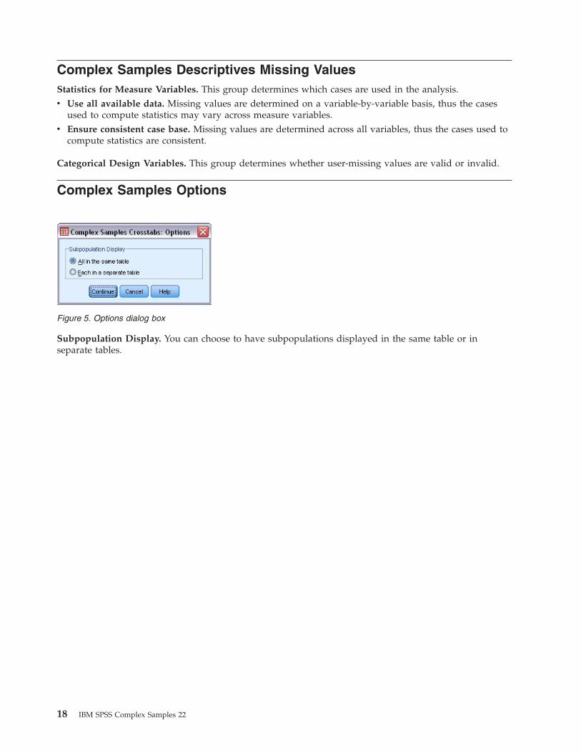
Complex Samples Options
Subpopulation Display. You can choose to have subpopulations displayed in the same table or inseparate tables.
Figure 5. Options dialog box
18 IBM SPSS Complex Samples 22
Chapter 7. Complex Samples Crosstabs
The Complex Samples Crosstabs procedure produces crosstabulation tables for pairs of selected variablesand displays two-way statistics. Optionally, you can request statistics by subgroups, defined by one ormore categorical variables.
Example. Using the Complex Samples Crosstabs procedure, you can obtain cross-classification statisticsfor smoking frequency by vitamin usage of U.S. citizens, based on the results of the National HealthInterview Survey (NHIS) and with an appropriate analysis plan for this public-use data.
Statistics. The procedure produces estimates of cell population sizes and row, column, and tablepercentages, plus standard errors, confidence intervals, coefficients of variation, expected values, designeffects, square roots of design effects, residuals, adjusted residuals, and unweighted counts for eachestimate. The odds ratio, relative risk, and risk difference are computed for 2-by-2 tables. Additionally,Pearson and likelihood-ratio statistics are computed for the test of independence of the row and columnvariables.
Complex Samples Crosstabs Data Considerations
Data. Row and column variables should be categorical. Subpopulation variables can be string or numericbut should be categorical.
Assumptions. The cases in the data file represent a sample from a complex design that should beanalyzed according to the specifications in the file selected in the Complex Samples Plan dialog box.
Obtaining Complex Samples Crosstabs1. From the menus choose:
Analyze > Complex Samples > Crosstabs...
2. Select a plan file. Optionally, select a custom joint probabilities file.3. Click Continue.4. In the Complex Samples Crosstabs dialog box, select at least one row variable and one column
variable.
Optionally, you can specify variables to define subpopulations. Statistics are computed separately for eachsubpopulation.
Complex Samples Crosstabs StatisticsCells. This group allows you to request estimates of the cell population size and row, column, and tablepercentages.
Statistics. This group produces statistics associated with the population size and row, column, and tablepercentages.v Standard error. The standard error of the estimate.v Confidence interval. A confidence interval for the estimate, using the specified level.v Coefficient of variation. The ratio of the standard error of the estimate to the estimate.v Expected values. The expected value of the estimate, under the hypothesis of independence of the row
and column variable.v Unweighted count. The number of units used to compute the estimate.
© Copyright IBM Corporation 1989, 2013 19
v Design effect. The ratio of the variance of the estimate to the variance obtained by assuming that thesample is a simple random sample. This is a measure of the effect of specifying a complex design,where values further from 1 indicate greater effects.
v Square root of design effect. This is a measure of the effect of specifying a complex design, wherevalues further from 1 indicate greater effects.
v Residuals. The expected value is the number of cases that you would expect in the cell if there wereno relationship between the two variables. A positive residual indicates that there are more cases in thecell than there would be if the row and column variables were independent.
v Adjusted residuals. The residual for a cell (observed minus expected value) divided by an estimate ofits standard error. The resulting standardized residual is expressed in standard deviation units above orbelow the mean.
Summaries for 2-by-2 Tables. This group produces statistics for tables in which the row and columnvariable each have two categories. Each is a measure of the strength of the association between thepresence of a factor and the occurrence of an event.v Odds ratio. The odds ratio can be used as an estimate of relative risk when the occurrence of the factor
is rare.v Relative risk. The ratio of the risk of an event in the presence of the factor to the risk of the event in
the absence of the factor.v Risk difference. The difference between the risk of an event in the presence of the factor and the risk
of the event in the absence of the factor.
Test of independence of rows and columns. This produces chi-square and likelihood-ratio tests of thehypothesis that a row and column variable are independent. Separate tests are performed for each pair ofvariables.
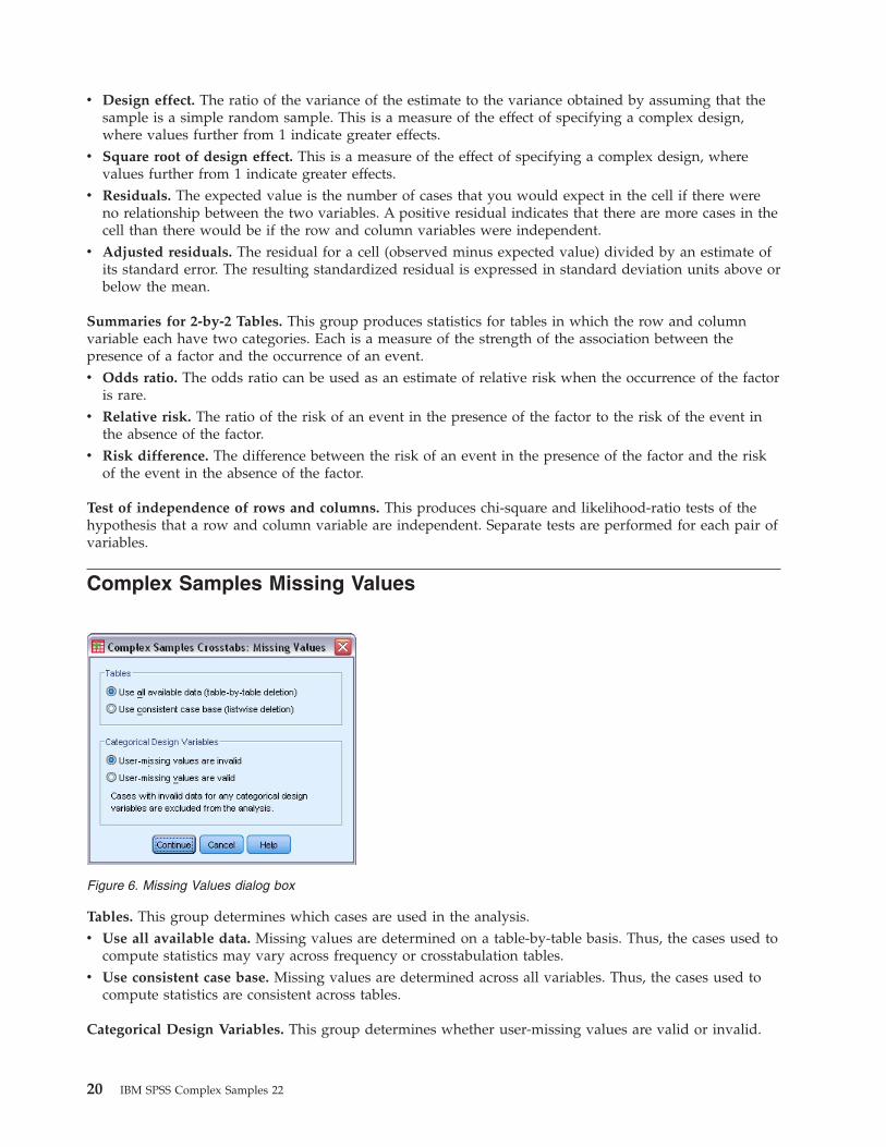
Complex Samples Missing Values
Tables. This group determines which cases are used in the analysis.v Use all available data. Missing values are determined on a table-by-table basis. Thus, the cases used to
compute statistics may vary across frequency or crosstabulation tables.v Use consistent case base. Missing values are determined across all variables. Thus, the cases used to
compute statistics are consistent across tables.
Categorical Design Variables. This group determines whether user-missing values are valid or invalid.
Figure 6. Missing Values dialog box
20 IBM SPSS Complex Samples 22
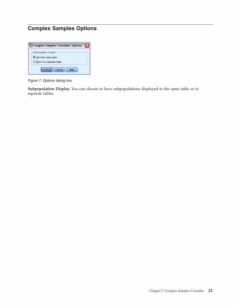
Complex Samples Options
Subpopulation Display. You can choose to have subpopulations displayed in the same table or inseparate tables.
Figure 7. Options dialog box
Chapter 7. Complex Samples Crosstabs 21

22 IBM SPSS Complex Samples 22
Chapter 8. Complex Samples Ratios
The Complex Samples Ratios procedure displays univariate summary statistics for ratios of variables.Optionally, you can request statistics by subgroups, defined by one or more categorical variables.
Example. Using the Complex Samples Ratios procedure, you can obtain descriptive statistics for the ratioof current property value to last assessed value, based on the results of a statewide survey carried outaccording to a complex design and with an appropriate analysis plan for the data.
Statistics. The procedure produces ratio estimates, t tests, standard errors, confidence intervals,coefficients of variation, unweighted counts, population sizes, design effects, and square roots of designeffects.
Complex Samples Ratios Data Considerations
Data. Numerators and denominators should be positive-valued scale variables. Subpopulation variablescan be string or numeric but should be categorical.
Assumptions. The cases in the data file represent a sample from a complex design that should beanalyzed according to the specifications in the file selected in the Complex Samples Plan dialog box.
Obtaining Complex Samples Ratios1. From the menus choose:
Analyze > Complex Samples > Ratios...
2. Select a plan file. Optionally, select a custom joint probabilities file.3. Click Continue.4. In the Complex Samples Ratios dialog box, select at least one numerator variable and denominator
variable.
Optionally, you can specify variables to define subgroups for which statistics are produced.
Complex Samples Ratios StatisticsStatistics. This group produces statistics associated with the ratio estimate.v Standard error. The standard error of the estimate.v Confidence interval. A confidence interval for the estimate, using the specified level.v Coefficient of variation. The ratio of the standard error of the estimate to the estimate.v Unweighted count. The number of units used to compute the estimate.v Population size. The estimated number of units in the population.v Design effect. The ratio of the variance of the estimate to the variance obtained by assuming that the
sample is a simple random sample. This is a measure of the effect of specifying a complex design,where values further from 1 indicate greater effects.
v Square root of design effect. This is a measure of the effect of specifying a complex design, wherevalues further from 1 indicate greater effects.
T test. You can request t tests of the estimates against a specified value.
Complex Samples Ratios Missing ValuesRatios. This group determines which cases are used in the analysis.
© Copyright IBM Corporation 1989, 2013 23

v Use all available data. Missing values are determined on a ratio-by-ratio basis. Thus, the cases used tocompute statistics may vary across numerator-denominator pairs.
v Ensure consistent case base. Missing values are determined across all variables. Thus, the cases usedto compute statistics are consistent.
Categorical Design Variables. This group determines whether user-missing values are valid or invalid.
Complex Samples Options
Subpopulation Display. You can choose to have subpopulations displayed in the same table or inseparate tables.
Figure 8. Options dialog box
24 IBM SPSS Complex Samples 22

Chapter 9. Complex Samples General Linear Model
The Complex Samples General Linear Model (CSGLM) procedure performs linear regression analysis, aswell as analysis of variance and covariance, for samples drawn by complex sampling methods.Optionally, you can request analyses for a subpopulation.
Example. A grocery store chain surveyed a set of customers concerning their purchasing habits, accordingto a complex design. Given the survey results and how much each customer spent in the previous month,the store wants to see if the frequency with which customers shop is related to the amount they spend ina month, controlling for the gender of the customer and incorporating the sampling design.
Statistics. The procedure produces estimates, standard errors, confidence intervals, t tests, design effects,and square roots of design effects for model parameters, as well as the correlations and covariancesbetween parameter estimates. Measures of model fit and descriptive statistics for the dependent andindependent variables are also available. Additionally, you can request estimated marginal means forlevels of model factors and factor interactions.
Complex Samples General Linear Model Data Considerations
Data. The dependent variable is quantitative. Factors are categorical. Covariates are quantitative variablesthat are related to the dependent variable. Subpopulation variables can be string or numeric but shouldbe categorical.
Assumptions. The cases in the data file represent a sample from a complex design that should beanalyzed according to the specifications in the file selected in the Complex Samples Plan dialog box.
Obtaining a Complex Samples General Linear Model1. From the menus choose:
Analyze > Complex Samples > General Linear Model...
2. Select a plan file. Optionally, select a custom joint probabilities file.3. Click Continue.4. In the Complex Samples General Linear Model dialog box, select a dependent variable.
Optionally, you can:v Select variables for factors and covariates, as appropriate for your data.v Specify a variable to define a subpopulation. The analysis is performed only for the selected category
of the subpopulation variable.
Complex Samples General Linear ModelSpecify Model Effects. By default, the procedure builds a main-effects model using the factors andcovariates specified in the main dialog box. Alternatively, you can build a custom model that includesinteraction effects and nested terms.
Non-Nested Terms
For the selected factors and covariates:
Interaction. Creates the highest-level interaction term for all selected variables.
Main effects. Creates a main-effects term for each variable selected.
© Copyright IBM Corporation 1989, 2013 25
All 2-way. Creates all possible two-way interactions of the selected variables.
All 3-way. Creates all possible three-way interactions of the selected variables.
All 4-way. Creates all possible four-way interactions of the selected variables.
All 5-way. Creates all possible five-way interactions of the selected variables.
Nested Terms
You can build nested terms for your model in this procedure. Nested terms are useful for modeling theeffect of a factor or covariate whose values do not interact with the levels of another factor. For example,a grocery store chain may follow the spending habits of its customers at several store locations. Sinceeach customer frequents only one of these locations, the Customer effect can be said to be nested withinthe Store location effect.
Additionally, you can include interaction effects, such as polynomial terms involving the same covariate,or add multiple levels of nesting to the nested term.
Limitations. Nested terms have the following restrictions:v All factors within an interaction must be unique. Thus, if A is a factor, then specifying A*A is invalid.v All factors within a nested effect must be unique. Thus, if A is a factor, then specifying A(A) is invalid.v No effect can be nested within a covariate. Thus, if A is a factor and X is a covariate, then specifying
A(X) is invalid.
Intercept. The intercept is usually included in the model. If you can assume the data pass through theorigin, you can exclude the intercept. Even if you include the intercept in the model, you can choose tosuppress statistics related to it.
Complex Samples General Linear Model StatisticsModel Parameters. This group allows you to control the display of statistics related to the modelparameters.v Estimate. Displays estimates of the coefficients.v Standard error. Displays the standard error for each coefficient estimate.v Confidence interval. Displays a confidence interval for each coefficient estimate. The confidence level
for the interval is set in the Options dialog box.v T test. Displays a t test of each coefficient estimate. The null hypothesis for each test is that the value
of the coefficient is 0.v Covariances of parameter estimates. Displays an estimate of the covariance matrix for the model
coefficients.v Correlations of parameter estimates. Displays an estimate of the correlation matrix for the model
coefficients.v Design effect. The ratio of the variance of the estimate to the variance obtained by assuming that the
sample is a simple random sample. This is a measure of the effect of specifying a complex design,where values further from 1 indicate greater effects.
v Square root of design effect. This is a measure of the effect of specifying a complex design, wherevalues further from 1 indicate greater effects.
Model fit. Displays R 2 and root mean squared error statistics.
Population means of dependent variable and covariates. Displays summary information about thedependent variable, covariates, and factors.
26 IBM SPSS Complex Samples 22

Sample design information. Displays summary information about the sample, including the unweightedcount and the population size.
Complex Samples Hypothesis Tests
Test Statistic. This group allows you to select the type of statistic used for testing hypotheses. You canchoose between F, adjusted F, chi-square, and adjusted chi-square.
Sampling Degrees of Freedom. This group gives you control over the sampling design degrees offreedom used to compute p values for all test statistics. If based on the sampling design, the value is thedifference between the number of primary sampling units and the number of strata in the first stage ofsampling. Alternatively, you can set a custom degrees of freedom by specifying a positive integer.
Adjustment for Multiple Comparisons. When performing hypothesis tests with multiple contrasts, theoverall significance level can be adjusted from the significance levels for the included contrasts. Thisgroup allows you to choose the adjustment method.v Least significant difference. This method does not control the overall probability of rejecting the
hypotheses that some linear contrasts are different from the null hypothesis values.v Sequential Sidak. This is a sequentially step-down rejective Sidak procedure that is much less
conservative in terms of rejecting individual hypotheses but maintains the same overall significancelevel.
v Sequential Bonferroni. This is a sequentially step-down rejective Bonferroni procedure that is much lessconservative in terms of rejecting individual hypotheses but maintains the same overall significancelevel.
v Sidak. This method provides tighter bounds than the Bonferroni approach.v Bonferroni. This method adjusts the observed significance level for the fact that multiple contrasts are
being tested.
Complex Samples General Linear Model Estimated MeansThe Estimated Means dialog box allows you to display the model-estimated marginal means for levels offactors and factor interactions specified in the Model subdialog box. You can also request that the overallpopulation mean be displayed.
Term. Estimated means are computed for the selected factors and factor interactions.
Contrast. The contrast determines how hypothesis tests are set up to compare the estimated means.v Simple. Compares the mean of each level to the mean of a specified level. This type of contrast is
useful when there is a control group.v Deviation. Compares the mean of each level (except a reference category) to the mean of all of the
levels (grand mean). The levels of the factor can be in any order.v Difference. Compares the mean of each level (except the first) to the mean of previous levels. They are
sometimes called reverse Helmert contrasts.v Helmert. Compares the mean of each level of the factor (except the last) to the mean of subsequent
levels.v Repeated. Compares the mean of each level (except the last) to the mean of the subsequent level.v Polynomial. Compares the linear effect, quadratic effect, cubic effect, and so on. The first degree of
freedom contains the linear effect across all categories; the second degree of freedom, the quadraticeffect; and so on. These contrasts are often used to estimate polynomial trends.
Reference Category. The simple and deviation contrasts require a reference category or factor levelagainst which the others are compared.
Chapter 9. Complex Samples General Linear Model 27
Complex Samples General Linear Model SaveSave Variables. This group allows you to save the model predicted values and residuals as new variablesin the working file.
Export model as IBM SPSS Statistics data. Writes a dataset in IBM SPSS Statistics format containing theparameter correlation or covariance matrix with parameter estimates, standard errors, significance values,and degrees of freedom. The order of variables in the matrix file is as follows.v rowtype_. Takes values (and value labels), COV (Covariances), CORR (Correlations), EST (Parameter
estimates), SE (Standard errors), SIG (Significance levels), and DF (Sampling design degrees offreedom). There is a separate case with row type COV (or CORR) for each model parameter, plus aseparate case for each of the other row types.
v varname_. Takes values P1, P2, ..., corresponding to an ordered list of all model parameters, for rowtypes COV or CORR, with value labels corresponding to the parameter strings shown in the parameterestimates table. The cells are blank for other row types.
v P1, P2, ... These variables correspond to an ordered list of all model parameters, with variable labelscorresponding to the parameter strings shown in the parameter estimates table, and take valuesaccording to the row type. For redundant parameters, all covariances are set to zero; correlations areset to the system-missing value; all parameter estimates are set at zero; and all standard errors,significance levels, and residual degrees of freedom are set to the system-missing value.
Note: This file is not immediately usable for further analyses in other procedures that read a matrix fileunless those procedures accept all the row types exported here.
Export Model as XML. Saves the parameter estimates and the parameter covariance matrix, if selected, inXML (PMML) format. You can use this model file to apply the model information to other data files forscoring purposes.
Complex Samples General Linear Model OptionsUser-Missing Values. All design variables, as well as the dependent variable and any covariates, musthave valid data. Cases with invalid data for any of these variables are deleted from the analysis. Thesecontrols allow you to decide whether user-missing values are treated as valid among the strata, cluster,subpopulation, and factor variables.
Confidence Interval. This is the confidence interval level for coefficient estimates and estimated marginalmeans. Specify a value greater than or equal to 50 and less than 100.
CSGLM Command Additional FeaturesThe command syntax language also allows you to:v Specify custom tests of effects versus a linear combination of effects or a value (using the CUSTOM
subcommand).v Fix covariates at values other than their means when computing estimated marginal means (using the
EMMEANS subcommand).v Specify a metric for polynomial contrasts (using the EMMEANS subcommand).v Specify a tolerance value for checking singularity (using the CRITERIA subcommand).v Create user-specified names for saved variables (using the SAVE subcommand).v Produce a general estimable function table (using the PRINT subcommand).
See the Command Syntax Reference for complete syntax information.
28 IBM SPSS Complex Samples 22

Chapter 10. Complex Samples Logistic Regression
The Complex Samples Logistic Regression procedure performs logistic regression analysis on a binary ormultinomial dependent variable for samples drawn by complex sampling methods. Optionally, you canrequest analyses for a subpopulation.
Example. A loan officer has collected past records of customers given loans at several different branches,according to a complex design. While incorporating the sample design, the officer wants to see if theprobability with which a customer defaults is related to age, employment history, and amount of creditdebt.
Statistics. The procedure produces estimates, exponentiated estimates, standard errors, confidenceintervals, t tests, design effects, and square roots of design effects for model parameters, as well as thecorrelations and covariances between parameter estimates. Pseudo R 2 statistics, classification tables, anddescriptive statistics for the dependent and independent variables are also available.
Complex Samples Logistic Regression Data Considerations
Data. The dependent variable is categorical. Factors are categorical. Covariates are quantitative variablesthat are related to the dependent variable. Subpopulation variables can be string or numeric but shouldbe categorical.
Assumptions. The cases in the data file represent a sample from a complex design that should beanalyzed according to the specifications in the file selected in the Complex Samples Plan dialog box.
Obtaining Complex Samples Logistic Regression1. From the menus choose:
Analyze > Complex Samples > Logistic Regression...
2. Select a plan file. Optionally, select a custom joint probabilities file.3. Click Continue.4. In the Complex Samples Logistic Regression dialog box, select a dependent variable.
Optionally, you can:v Select variables for factors and covariates, as appropriate for your data.v Specify a variable to define a subpopulation. The analysis is performed only for the selected category
of the subpopulation variable.
Complex Samples Logistic Regression Reference CategoryBy default, the Complex Samples Logistic Regression procedure makes the highest-valued category thereference category. This dialog box allows you to specify the highest value, the lowest value, or a customcategory as the reference category.
Complex Samples Logistic Regression ModelSpecify Model Effects. By default, the procedure builds a main-effects model using the factors andcovariates specified in the main dialog box. Alternatively, you can build a custom model that includesinteraction effects and nested terms.
Non-Nested Terms
© Copyright IBM Corporation 1989, 2013 29
For the selected factors and covariates:
Interaction. Creates the highest-level interaction term for all selected variables.
Main effects. Creates a main-effects term for each variable selected.
All 2-way. Creates all possible two-way interactions of the selected variables.
All 3-way. Creates all possible three-way interactions of the selected variables.
All 4-way. Creates all possible four-way interactions of the selected variables.
All 5-way. Creates all possible five-way interactions of the selected variables.
Nested Terms
You can build nested terms for your model in this procedure. Nested terms are useful for modeling theeffect of a factor or covariate whose values do not interact with the levels of another factor. For example,a grocery store chain may follow the spending habits of its customers at several store locations. Sinceeach customer frequents only one of these locations, the Customer effect can be said to be nested withinthe Store location effect.
Additionally, you can include interaction effects, such as polynomial terms involving the same covariate,or add multiple levels of nesting to the nested term.
Limitations. Nested terms have the following restrictions:v All factors within an interaction must be unique. Thus, if A is a factor, then specifying A*A is invalid.v All factors within a nested effect must be unique. Thus, if A is a factor, then specifying A(A) is invalid.v No effect can be nested within a covariate. Thus, if A is a factor and X is a covariate, then specifying
A(X) is invalid.
Intercept. The intercept is usually included in the model. If you can assume the data pass through theorigin, you can exclude the intercept. Even if you include the intercept in the model, you can choose tosuppress statistics related to it.
Complex Samples Logistic Regression StatisticsModel Fit. Controls the display of statistics that measure the overall model performance.v Pseudo R-square. The R 2 statistic from linear regression does not have an exact counterpart among
logistic regression models. There are, instead, multiple measures that attempt to mimic the propertiesof the R 2 statistic.
v Classification table. Displays the tabulated cross-classifications of the observed category by themodel-predicted category on the dependent variable.
Parameters. This group allows you to control the display of statistics related to the model parameters.v Estimate. Displays estimates of the coefficients.v Exponentiated estimate. Displays the base of the natural logarithm raised to the power of the
estimates of the coefficients. While the estimate has nice properties for statistical testing, theexponentiated estimate, or exp(B), is easier to interpret.
v Standard error. Displays the standard error for each coefficient estimate.v Confidence interval. Displays a confidence interval for each coefficient estimate. The confidence level
for the interval is set in the Options dialog box.
30 IBM SPSS Complex Samples 22

v T test. Displays a t test of each coefficient estimate. The null hypothesis for each test is that the valueof the coefficient is 0.
v Covariances of parameter estimates. Displays an estimate of the covariance matrix for the modelcoefficients.
v Correlations of parameter estimates. Displays an estimate of the correlation matrix for the modelcoefficients.
v Design effect. The ratio of the variance of the estimate to the variance obtained by assuming that thesample is a simple random sample. This is a measure of the effect of specifying a complex design,where values further from 1 indicate greater effects.
v Square root of design effect. This is a measure of the effect of specifying a complex design, wherevalues further from 1 indicate greater effects.
Summary statistics for model variables. Displays summary information about the dependent variable,covariates, and factors.
Sample design information. Displays summary information about the sample, including the unweightedcount and the population size.
Complex Samples Hypothesis Tests
Test Statistic. This group allows you to select the type of statistic used for testing hypotheses. You canchoose between F, adjusted F, chi-square, and adjusted chi-square.
Sampling Degrees of Freedom. This group gives you control over the sampling design degrees offreedom used to compute p values for all test statistics. If based on the sampling design, the value is thedifference between the number of primary sampling units and the number of strata in the first stage ofsampling. Alternatively, you can set a custom degrees of freedom by specifying a positive integer.
Adjustment for Multiple Comparisons. When performing hypothesis tests with multiple contrasts, theoverall significance level can be adjusted from the significance levels for the included contrasts. Thisgroup allows you to choose the adjustment method.v Least significant difference. This method does not control the overall probability of rejecting the
hypotheses that some linear contrasts are different from the null hypothesis values.v Sequential Sidak. This is a sequentially step-down rejective Sidak procedure that is much less
conservative in terms of rejecting individual hypotheses but maintains the same overall significancelevel.
v Sequential Bonferroni. This is a sequentially step-down rejective Bonferroni procedure that is much lessconservative in terms of rejecting individual hypotheses but maintains the same overall significancelevel.
v Sidak. This method provides tighter bounds than the Bonferroni approach.v Bonferroni. This method adjusts the observed significance level for the fact that multiple contrasts are
being tested.
Complex Samples Logistic Regression Odds RatiosThe Odds Ratios dialog box allows you to display the model-estimated odds ratios for specified factorsand covariates. A separate set of odds ratios is computed for each category of the dependent variableexcept the reference category.
Factors. For each selected factor, displays the ratio of the odds at each category of the factor to the oddsat the specified reference category.
Chapter 10. Complex Samples Logistic Regression 31

Covariates. For each selected covariate, displays the ratio of the odds at the covariate's mean value plusthe specified units of change to the odds at the mean.
When computing odds ratios for a factor or covariate, the procedure fixes all other factors at their highestlevels and all other covariates at their means. If a factor or covariate interacts with other predictors in themodel, then the odds ratios depend not only on the change in the specified variable but also on thevalues of the variables with which it interacts. If a specified covariate interacts with itself in the model(for example, age*age), then the odds ratios depend on both the change in the covariate and the value ofthe covariate.
Complex Samples Logistic Regression SaveSave Variables. This group allows you to save the model-predicted category and predicted probabilitiesas new variables in the active dataset.
Export model as IBM SPSS Statistics data. Writes a dataset in IBM SPSS Statistics format containing theparameter correlation or covariance matrix with parameter estimates, standard errors, significance values,and degrees of freedom. The order of variables in the matrix file is as follows.v rowtype_. Takes values (and value labels), COV (Covariances), CORR (Correlations), EST (Parameter
estimates), SE (Standard errors), SIG (Significance levels), and DF (Sampling design degrees offreedom). There is a separate case with row type COV (or CORR) for each model parameter, plus aseparate case for each of the other row types.
v varname_. Takes values P1, P2, ..., corresponding to an ordered list of all model parameters, for rowtypes COV or CORR, with value labels corresponding to the parameter strings shown in the parameterestimates table. The cells are blank for other row types.
v P1, P2, ... These variables correspond to an ordered list of all model parameters, with variable labelscorresponding to the parameter strings shown in the parameter estimates table, and take valuesaccording to the row type. For redundant parameters, all covariances are set to zero; correlations areset to the system-missing value; all parameter estimates are set at zero; and all standard errors,significance levels, and residual degrees of freedom are set to the system-missing value.
Note: This file is not immediately usable for further analyses in other procedures that read a matrix fileunless those procedures accept all the row types exported here.
Export Model as XML. Saves the parameter estimates and the parameter covariance matrix, if selected, inXML (PMML) format. You can use this model file to apply the model information to other data files forscoring purposes.
Complex Samples Logistic Regression OptionsEstimation. This group gives you control of various criteria used in the model estimation.v Maximum Iterations. The maximum number of iterations the algorithm will execute. Specify a
non-negative integer.v Maximum Step-Halving. At each iteration, the step size is reduced by a factor of 0.5 until the
log-likelihood increases or maximum step-halving is reached. Specify a positive integer.v Limit iterations based on change in parameter estimates. When selected, the algorithm stops after an
iteration in which the absolute or relative change in the parameter estimates is less than the valuespecified, which must be non-negative.
v Limit iterations based on change in log-likelihood. When selected, the algorithm stops after aniteration in which the absolute or relative change in the log-likelihood function is less than the valuespecified, which must be non-negative.
v Check for complete separation of data points. When selected, the algorithm performs tests to ensurethat the parameter estimates have unique values. Separation occurs when the procedure can produce amodel that correctly classifies every case.
32 IBM SPSS Complex Samples 22

v Display iteration history. Displays parameter estimates and statistics at every n iterations beginningwith the 0th iteration (the initial estimates). If you choose to print the iteration history, the last iterationis always printed regardless of the value of n.
User-Missing Values. All design variables, as well as the dependent variable and any covariates, musthave valid data. Cases with invalid data for any of these variables are deleted from the analysis. Thesecontrols allow you to decide whether user-missing values are treated as valid among the strata, cluster,subpopulation, and factor variables.
Confidence Interval. This is the confidence interval level for coefficient estimates, exponentiatedcoefficient estimates, and odds ratios. Specify a value greater than or equal to 50 and less than 100.
CSLOGISTIC Command Additional FeaturesThe command syntax language also allows you to:v Specify custom tests of effects versus a linear combination of effects or a value (using the CUSTOM
subcommand).v Fix values of other model variables when computing odds ratios for factors and covariates (using the
ODDSRATIOS subcommand).v Specify a tolerance value for checking singularity (using the CRITERIA subcommand).v Create user-specified names for saved variables (using the SAVE subcommand).v Produce a general estimable function table (using the PRINT subcommand).
See the Command Syntax Reference for complete syntax information.
Chapter 10. Complex Samples Logistic Regression 33

34 IBM SPSS Complex Samples 22

Chapter 11. Complex Samples Ordinal Regression
The Complex Samples Ordinal Regression procedure performs regression analysis on a binary or ordinaldependent variable for samples drawn by complex sampling methods. Optionally, you can requestanalyses for a subpopulation.
Example. Representatives considering a bill before the legislature are interested in whether there is publicsupport for the bill and how support for the bill is related to voter demographics. Pollsters design andconduct interviews according to a complex sampling design. Using Complex Samples Ordinal Regression,you can fit a model for the level of support for the bill based upon voter demographics.
Complex Samples Ordinal Regression Data Considerations
Data. The dependent variable is ordinal. Factors are categorical. Covariates are quantitative variables thatare related to the dependent variable. Subpopulation variables can be string or numeric but should becategorical.
Assumptions. The cases in the data file represent a sample from a complex design that should beanalyzed according to the specifications in the file selected in the Complex Samples Plan dialog box.
Obtaining Complex Samples Ordinal Regression1. From the menus choose:
Analyze > Complex Samples > Ordinal Regression...
2. Select a plan file. Optionally, select a custom joint probabilities file.3. Click Continue.4. In the Complex Samples Ordinal Regression dialog box, select a dependent variable.
Optionally, you can:v Select variables for factors and covariates, as appropriate for your data.v Specify a variable to define a subpopulation. The analysis is performed only for the selected category
of the subpopulation variable, although variances are still properly estimated based on the entiredataset.
v Select a link function.
Link function. The link function is a transformation of the cumulative probabilities that allows estimationof the model. The following five link functions are available.v Logit. f(x)=log(x/(1−x) ). Typically used for evenly distributed categories.v Complementary log-log. f(x)=log(−log(1−x)). Typically used when higher categories are more probable.v Negative log-log. f(x)=−log(−log(x)). Typically used when lower categories are more probable.v Probit. f(x)=Φ−1(x). Typically used when the latent variable is normally distributed.v Cauchit (inverse Cauchy). f(x)=tan(π(x−0.5)). Typically used when the latent variable has many
extreme values.
Complex Samples Ordinal Regression Response ProbabilitiesThe Response Probabilities dialog box allows you to specify whether the cumulative probability of aresponse (that is, the probability of belonging up to and including a particular category of the dependentvariable) increases with increasing or decreasing values of the dependent variable.
© Copyright IBM Corporation 1989, 2013 35

Complex Samples Ordinal Regression ModelSpecify Model Effects. By default, the procedure builds a main-effects model using the factors andcovariates specified in the main dialog box. Alternatively, you can build a custom model that includesinteraction effects and nested terms.
Non-Nested Terms
For the selected factors and covariates:
Interaction. Creates the highest-level interaction term for all selected variables.
Main effects. Creates a main-effects term for each variable selected.
All 2-way. Creates all possible two-way interactions of the selected variables.
All 3-way. Creates all possible three-way interactions of the selected variables.
All 4-way. Creates all possible four-way interactions of the selected variables.
All 5-way. Creates all possible five-way interactions of the selected variables.
Nested Terms
You can build nested terms for your model in this procedure. Nested terms are useful for modeling theeffect of a factor or covariate whose values do not interact with the levels of another factor. For example,a grocery store chain may follow the spending habits of its customers at several store locations. Sinceeach customer frequents only one of these locations, the Customer effect can be said to be nested withinthe Store location effect.
Additionally, you can include interaction effects, such as polynomial terms involving the same covariate,or add multiple levels of nesting to the nested term.
Limitations. Nested terms have the following restrictions:v All factors within an interaction must be unique. Thus, if A is a factor, then specifying A*A is invalid.v All factors within a nested effect must be unique. Thus, if A is a factor, then specifying A(A) is invalid.v No effect can be nested within a covariate. Thus, if A is a factor and X is a covariate, then specifying
A(X) is invalid.
Complex Samples Ordinal Regression StatisticsModel Fit. Controls the display of statistics that measure the overall model performance.v Pseudo R-square. The R 2 statistic from linear regression does not have an exact counterpart among
ordinal regression models. There are, instead, multiple measures that attempt to mimic the propertiesof the R 2 statistic.
v Classification table. Displays the tabulated cross-classifications of the observed category by themodel-predicted category on the dependent variable.
Parameters. This group allows you to control the display of statistics related to the model parameters.v Estimate. Displays estimates of the coefficients.v Exponentiated estimate. Displays the base of the natural logarithm raised to the power of the
estimates of the coefficients. While the estimate has nice properties for statistical testing, theexponentiated estimate, or exp(B), is easier to interpret.
v Standard error. Displays the standard error for each coefficient estimate.
36 IBM SPSS Complex Samples 22

v Confidence interval. Displays a confidence interval for each coefficient estimate. The confidence levelfor the interval is set in the Options dialog box.
v T test. Displays a t test of each coefficient estimate. The null hypothesis for each test is that the valueof the coefficient is 0.
v Covariances of parameter estimates. Displays an estimate of the covariance matrix for the modelcoefficients.
v Correlations of parameter estimates. Displays an estimate of the correlation matrix for the modelcoefficients.
v Design effect. The ratio of the variance of the estimate to the variance obtained by assuming that thesample is a simple random sample. This is a measure of the effect of specifying a complex design,where values further from 1 indicate greater effects.
v Square root of design effect. This is a measure, expressed in units comparable to those of the standarderror, of the effect of specifying a complex design, where values further from 1 indicate greater effects.
Parallel Lines. This group allows you to request statistics associated with a model with nonparallel lineswhere a separate regression line is fitted for each response category (except the last).v Wald test. Produces a test of the null hypothesis that regression parameters are equal for all cumulative
responses. The model with nonparallel lines is estimated and the Wald test of equal parameters isapplied.
v Parameter estimates. Displays estimates of the coefficients and standard errors for the model withnonparallel lines.
v Covariances of parameter estimates. Displays an estimate of the covariance matrix for the coefficientsof the model with nonparallel lines.
Summary statistics for model variables. Displays summary information about the dependent variable,covariates, and factors.
Sample design information. Displays summary information about the sample, including the unweightedcount and the population size.
Complex Samples Hypothesis Tests
Test Statistic. This group allows you to select the type of statistic used for testing hypotheses. You canchoose between F, adjusted F, chi-square, and adjusted chi-square.
Sampling Degrees of Freedom. This group gives you control over the sampling design degrees offreedom used to compute p values for all test statistics. If based on the sampling design, the value is thedifference between the number of primary sampling units and the number of strata in the first stage ofsampling. Alternatively, you can set a custom degrees of freedom by specifying a positive integer.
Adjustment for Multiple Comparisons. When performing hypothesis tests with multiple contrasts, theoverall significance level can be adjusted from the significance levels for the included contrasts. Thisgroup allows you to choose the adjustment method.v Least significant difference. This method does not control the overall probability of rejecting the
hypotheses that some linear contrasts are different from the null hypothesis values.v Sequential Sidak. This is a sequentially step-down rejective Sidak procedure that is much less
conservative in terms of rejecting individual hypotheses but maintains the same overall significancelevel.
v Sequential Bonferroni. This is a sequentially step-down rejective Bonferroni procedure that is much lessconservative in terms of rejecting individual hypotheses but maintains the same overall significancelevel.
v Sidak. This method provides tighter bounds than the Bonferroni approach.
Chapter 11. Complex Samples Ordinal Regression 37
v Bonferroni. This method adjusts the observed significance level for the fact that multiple contrasts arebeing tested.
Complex Samples Ordinal Regression Odds RatiosThe Odds Ratios dialog box allows you to display the model-estimated cumulative odds ratios forspecified factors and covariates. This feature is only available for models using the Logit link function. Asingle cumulative odds ratio is computed for all categories of the dependent variable except the last; theproportional odds model postulates that they are all equal.
Factors. For each selected factor, displays the ratio of the cumulative odds at each category of the factorto the odds at the specified reference category.
Covariates. For each selected covariate, displays the ratio of the cumulative odds at the covariate's meanvalue plus the specified units of change to the odds at the mean.
When computing odds ratios for a factor or covariate, the procedure fixes all other factors at their highestlevels and all other covariates at their means. If a factor or covariate interacts with other predictors in themodel, then the odds ratios depend not only on the change in the specified variable but also on thevalues of the variables with which it interacts. If a specified covariate interacts with itself in the model(for example, age*age), then the odds ratios depend on both the change in the covariate and the value ofthe covariate.
Complex Samples Ordinal Regression SaveSave Variables. This group allows you to save the model-predicted category, probability of predictedcategory, probability of observed category, cumulative probabilities, and predicted probabilities as newvariables in the active dataset.
Export model as IBM SPSS Statistics data. Writes a dataset in IBM SPSS Statistics format containing theparameter correlation or covariance matrix with parameter estimates, standard errors, significance values,and degrees of freedom. The order of variables in the matrix file is as follows.v rowtype_. Takes values (and value labels), COV (Covariances), CORR (Correlations), EST (Parameter
estimates), SE (Standard errors), SIG (Significance levels), and DF (Sampling design degrees offreedom). There is a separate case with row type COV (or CORR) for each model parameter, plus aseparate case for each of the other row types.
v varname_. Takes values P1, P2, ..., corresponding to an ordered list of all model parameters, for rowtypes COV or CORR, with value labels corresponding to the parameter strings shown in the parameterestimates table. The cells are blank for other row types.
v P1, P2, ... These variables correspond to an ordered list of all model parameters, with variable labelscorresponding to the parameter strings shown in the parameter estimates table, and take valuesaccording to the row type. For redundant parameters, all covariances are set to zero; correlations areset to the system-missing value; all parameter estimates are set at zero; and all standard errors,significance levels, and residual degrees of freedom are set to the system-missing value.
Note: This file is not immediately usable for further analyses in other procedures that read a matrix fileunless those procedures accept all the row types exported here.
Export model as XML. Saves the parameter estimates and the parameter covariance matrix, if selected, inXML (PMML) format. You can use this model file to apply the model information to other data files forscoring purposes.
38 IBM SPSS Complex Samples 22
Complex Samples Ordinal Regression OptionsEstimation Method. You can select a parameter estimation method; choose between Newton-Raphson,Fisher scoring, or a hybrid method in which Fisher scoring iterations are performed before switching tothe Newton-Raphson method. If convergence is achieved during the Fisher scoring phase of the hybridmethod before the maximum number of Fisher iterations is reached, the algorithm continues with theNewton-Raphson method.
Estimation. This group gives you control of various criteria used in the model estimation.v Maximum Iterations. The maximum number of iterations the algorithm will execute. Specify a
non-negative integer.v Maximum Step-Halving. At each iteration, the step size is reduced by a factor of 0.5 until the
log-likelihood increases or maximum step-halving is reached. Specify a positive integer.v Limit iterations based on change in parameter estimates. When selected, the algorithm stops after an
iteration in which the absolute or relative change in the parameter estimates is less than the valuespecified, which must be non-negative.
v Limit iterations based on change in log-likelihood. When selected, the algorithm stops after aniteration in which the absolute or relative change in the log-likelihood function is less than the valuespecified, which must be non-negative.
v Check for complete separation of data points. When selected, the algorithm performs tests to ensurethat the parameter estimates have unique values. Separation occurs when the procedure can produce amodel that correctly classifies every case.
v Display iteration history. Displays parameter estimates and statistics at every n iterations beginningwith the 0th iteration (the initial estimates). If you choose to print the iteration history, the last iterationis always printed regardless of the value of n.
User-Missing Values. Scale design variables, as well as the dependent variable and any covariates,should have valid data. Cases with invalid data for any of these variables are deleted from the analysis.These controls allow you to decide whether user-missing values are treated as valid among the strata,cluster, subpopulation, and factor variables.
Confidence Interval. This is the confidence interval level for coefficient estimates, exponentiatedcoefficient estimates, and odds ratios. Specify a value greater than or equal to 50 and less than 100.
CSORDINAL Command Additional FeaturesThe command syntax language also allows you to:v Specify custom tests of effects versus a linear combination of effects or a value (using the CUSTOM
subcommand).v Fix values of other model variables at values other than their means when computing cumulative odds
ratios for factors and covariates (using the ODDSRATIOS subcommand).v Use unlabeled values as custom reference categories for factors when odds ratios are requested (using
the ODDSRATIOS subcommand).v Specify a tolerance value for checking singularity (using the CRITERIA subcommand).v Produce a general estimable function table (using the PRINT subcommand).v Save more than 25 probability variables (using the SAVE subcommand).
See the Command Syntax Reference for complete syntax information.
Chapter 11. Complex Samples Ordinal Regression 39

40 IBM SPSS Complex Samples 22

Chapter 12. Complex Samples Cox Regression
The Complex Samples Cox Regression procedure performs survival analysis for samples drawn bycomplex sampling methods. Optionally, you can request analyses for a subpopulation.
Examples. A government law enforcement agency is concerned about recidivism rates in their area ofjurisdiction. One of the measures of recidivism is the time until second arrest for offenders. The agencywould like to model time to rearrest using Cox Regression but are worried the proportional hazardsassumption is invalid across age categories.
Medical researchers are investigating survival times for patients exiting a rehabilitation programpost-ischemic stroke. There is the potential for multiple cases per subject, since patient histories change asthe occurrence of significant nondeath events are noted and the times of these events recorded. Thesample is also left-truncated in the sense that the observed survival times are "inflated" by the length ofrehabilitation, because while the onset of risk starts at the time of the ischemic stroke, only patients whosurvive past the rehabilitation program are in the sample.
Complex Samples Cox Regression Data Considerations
Survival Time. The procedure applies Cox regression to analysis of survival times—that is, the length oftime before the occurrence of an event. There are two ways to specify the survival time, depending uponthe start time of the interval:v Time=0. Commonly, you will have complete information on the start of the interval for each subject
and will simply have a variable containing end times (or create a single variable with end times fromDate & Time variables; see below).
v Varies by subject. This is appropriate when you have left-truncation, also called delayed entry; forexample, if you are analyzing survival times for patients exiting a rehabilitation program post-stroke,you might consider that their onset of risk starts at the time of the stroke. However, if your sampleonly includes patients who have survived the rehabilitation program, then your sample isleft-truncated in the sense that the observed survival times are "inflated" by the length of rehabilitation.You can account for this by specifying the time at which they exited rehabilitation as the time of entryinto the study.
Date & Time Variables. Date & Time variables cannot be used to directly define the start and end of theinterval; if you have Date & Time variables, you should use them to create variables containing survivaltimes. If there is no left-truncation, simply create a variable containing end times based upon thedifference between the date of entry into the study and the observation date. If there is left-truncation,create a variable containing start times, based upon the difference between the date of the start of thestudy and the date of entry, and a variable containing end times, based upon the difference between thedate of the start of the study and the date of observation.
Event Status. You need a variable that records whether the subject experienced the event of interestwithin the interval. Subjects for whom the event has not occurred are right-censored.
Subject Identifier. You can easily incorporate piecewise-constant, time-dependent predictors by splittingthe observations for a single subject across multiple cases. For example, if you are analyzing survivaltimes for patients post-stroke, variables representing their medical history should be useful as predictors.Over time, they may experience major medical events that alter their medical history. The following tableshows how to structure such a dataset: Patient ID is the subject identifier, End time defines the observedintervals, Status records major medical events, and Prior history of heart attack and Prior history ofhemorrhaging are piecewise-constant, time-dependent predictors.
© Copyright IBM Corporation 1989, 2013 41
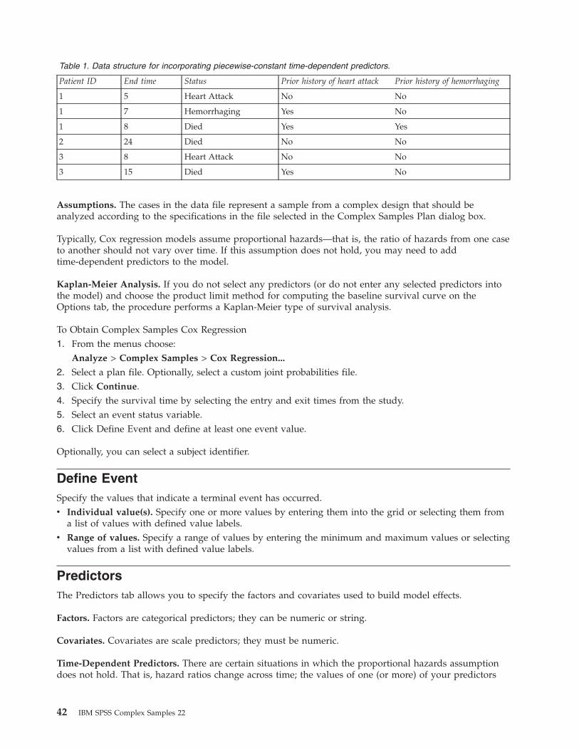
Table 1. Data structure for incorporating piecewise-constant time-dependent predictors.
Patient ID End time Status Prior history of heart attack Prior history of hemorrhaging
1 5 Heart Attack No No
1 7 Hemorrhaging Yes No
1 8 Died Yes Yes
2 24 Died No No
3 8 Heart Attack No No
3 15 Died Yes No
Assumptions. The cases in the data file represent a sample from a complex design that should beanalyzed according to the specifications in the file selected in the Complex Samples Plan dialog box.
Typically, Cox regression models assume proportional hazards—that is, the ratio of hazards from one caseto another should not vary over time. If this assumption does not hold, you may need to addtime-dependent predictors to the model.
Kaplan-Meier Analysis. If you do not select any predictors (or do not enter any selected predictors intothe model) and choose the product limit method for computing the baseline survival curve on theOptions tab, the procedure performs a Kaplan-Meier type of survival analysis.
To Obtain Complex Samples Cox Regression1. From the menus choose:
Analyze > Complex Samples > Cox Regression...
2. Select a plan file. Optionally, select a custom joint probabilities file.3. Click Continue.4. Specify the survival time by selecting the entry and exit times from the study.5. Select an event status variable.6. Click Define Event and define at least one event value.
Optionally, you can select a subject identifier.
Define EventSpecify the values that indicate a terminal event has occurred.v Individual value(s). Specify one or more values by entering them into the grid or selecting them from
a list of values with defined value labels.v Range of values. Specify a range of values by entering the minimum and maximum values or selecting
values from a list with defined value labels.
PredictorsThe Predictors tab allows you to specify the factors and covariates used to build model effects.
Factors. Factors are categorical predictors; they can be numeric or string.
Covariates. Covariates are scale predictors; they must be numeric.
Time-Dependent Predictors. There are certain situations in which the proportional hazards assumptiondoes not hold. That is, hazard ratios change across time; the values of one (or more) of your predictors
42 IBM SPSS Complex Samples 22
are different at different time points. In such cases, you need to specify time-dependent predictors. Seethe topic “Define Time-Dependent Predictor” for more information. Time-dependent predictors can beselected as factors or covariates.
Define Time-Dependent PredictorThe Define Time-Dependent Predictor dialog box allows you to create a predictor that is dependent uponthe built-in time variable, T_. You can use this variable to define time-dependent covariates in twogeneral ways:v If you want to estimate an extended Cox regression model that allows nonproportional hazards, you
can do so by defining your time-dependent predictor as a function of the time variable T_ and thecovariate in question. A common example would be the simple product of the time variable and thepredictor, but more complex functions can be specified as well.
v Some variables may have different values at different time periods but aren't systematically related totime. In such cases, you need to define a segmented time-dependent predictor, which can be doneusing logical expressions. Logical expressions take the value 1 if true and 0 if false. Using a series oflogical expressions, you can create your time-dependent predictor from a set of measurements. Forexample, if you have blood pressure measured once a week for the four weeks of your study(identified as BP1 to BP4), you can define your time-dependent predictor as (T_ < 1) * BP1 + (T_ >= 1& T_ < 2) * BP2 + (T_ >= 2 & T_ < 3) * BP3 + (T_ >= 3 & T_ < 4) * BP4. Notice that exactly one of theterms in parentheses will be equal to 1 for any given case and the rest will all equal 0. In other words,this function means that if time is less than one week, use BP1; if it is more than one week but lessthan two weeks, use BP2; and so on.Note: If your segmented, time-dependent predictor is constant within segments, as in the bloodpressure example given above, it may be easier for you to specify the piecewise-constant,time-dependent predictor by splitting subjects across multiple cases. See the discussion on SubjectIdentifiers in Chapter 12, “Complex Samples Cox Regression,” on page 41 for more information.
In the Define Time-Dependent Predictor dialog box, you can use the function-building controls to buildthe expression for the time-dependent covariate, or you can enter it directly in the Numeric Expressiontext area. Note that string constants must be enclosed in quotation marks or apostrophes, and numericconstants must be typed in American format, with the dot as the decimal delimiter. The resulting variableis given the name you specify and should be included as a factor or covariate on the Predictors tab.
SubgroupsBaseline Strata. A separate baseline hazard and survival function is computed for each value of thisvariable, while a single set of model coefficients is estimated across strata.
Subpopulation Variable. Specify a variable to define a subpopulation. The analysis is performed only forthe selected category of the subpopulation variable.
ModelSpecify Model Effects. By default, the procedure builds a main-effects model using the factors andcovariates specified in the main dialog box. Alternatively, you can build a custom model that includesinteraction effects and nested terms.
Non-Nested Terms
For the selected factors and covariates:
Interaction. Creates the highest-level interaction term for all selected variables.
Main effects. Creates a main-effects term for each variable selected.
Chapter 12. Complex Samples Cox Regression 43

All 2-way. Creates all possible two-way interactions of the selected variables.
All 3-way. Creates all possible three-way interactions of the selected variables.
All 4-way. Creates all possible four-way interactions of the selected variables.
All 5-way. Creates all possible five-way interactions of the selected variables.
Nested Terms
You can build nested terms for your model in this procedure. Nested terms are useful for modeling theeffect of a factor or covariate whose values do not interact with the levels of another factor. For example,a grocery store chain may follow the spending habits of its customers at several store locations. Sinceeach customer frequents only one of these locations, the Customer effect can be said to be nested withinthe Store location effect.
Additionally, you can include interaction effects, such as polynomial terms involving the same covariate,or add multiple levels of nesting to the nested term.
Limitations. Nested terms have the following restrictions:v All factors within an interaction must be unique. Thus, if A is a factor, then specifying A*A is invalid.v All factors within a nested effect must be unique. Thus, if A is a factor, then specifying A(A) is invalid.v No effect can be nested within a covariate. Thus, if A is a factor and X is a covariate, then specifying
A(X) is invalid.
StatisticsSample design information. Displays summary information about the sample, including the unweightedcount and the population size.
Event and censoring summary. Displays summary information about the number and percentage ofcensored cases.
Risk set at event times. Displays number of events and number at risk for each event time in eachbaseline stratum.
Parameters. This group allows you to control the display of statistics related to the model parameters.v Estimate. Displays estimates of the coefficients.v Exponentiated estimate. Displays the base of the natural logarithm raised to the power of the
estimates of the coefficients. While the estimate has nice properties for statistical testing, theexponentiated estimate, or exp(B), is easier to interpret.
v Standard error. Displays the standard error for each coefficient estimate.v Confidence interval. Displays a confidence interval for each coefficient estimate. The confidence level
for the interval is set in the Options dialog box.v t-test. Displays a t test of each coefficient estimate. The null hypothesis for each test is that the value of
the coefficient is 0.v Covariances of parameter estimates. Displays an estimate of the covariance matrix for the model
coefficients.v Correlations of parameter estimates. Displays an estimate of the correlation matrix for the model
coefficients.v Design effect. The ratio of the variance of the estimate to the variance obtained by assuming that the
sample is a simple random sample. This is a measure of the effect of specifying a complex design,where values further from 1 indicate greater effects.
44 IBM SPSS Complex Samples 22
v Square root of design effect. This is a measure of the effect of specifying a complex design, wherevalues further from 1 indicate greater effects.
Model Assumptions. This group allows you to produce a test of the proportional hazards assumption.The test compares the fitted model to an alternative model that includes time-dependent predictors x*_TFfor each predictor x, where _TF is the specified time function.v Time Function. Specifies the form of _TF for the alternative model. For the identity function, _TF=T_.
For the log function, _TF=log(T_). For Kaplan-Meier, _TF=1−S KM(T_), where S KM(.) is theKaplan-Meier estimate of the survival function. For rank, _TF is the rank-order of T_ among theobserved end times.
v Parameter estimates for alternative model. Displays the estimate, standard error, and confidenceinterval for each parameter in the alternative model.
v Covariance matrix for alternative model. Displays the matrix of estimated covariances betweenparameters in the alternative model.
Baseline survival and cumulative hazard functions. Displays the baseline survival function and baselinecumulative hazards function along with their standard errors.
Note: If time-dependent predictors defined on the Predictors tab are included in the model, this option isnot available.
PlotsThe Plots tab allows you to request plots of the hazard function, survival function, log-minus-log of thesurvival function, and one minus the survival function. You can also choose to plot confidence intervalsalong the specified functions; the confidence level is set on the Options tab.
Predictor patterns. You can specify a pattern of predictor values to be used for the requested plots andthe exported survival file on the Export tab. Note that these options are not available if time-dependentpredictors defined on the Predictors tab are included in the model.v Plot Factors at. By default, each factor is evaluated at its highest level. Enter or select a different level
if wanted. Alternatively, you can choose to plot separate lines for each level of a single factor byselecting the check box for that factor.
v Plot Covariates at. Each covariate is evaluated at its mean. Enter or select a different value if youwant.
Hypothesis TestsTest Statistic. This group allows you to select the type of statistic used for testing hypotheses. You canchoose between F, adjusted F, chi-square, and adjusted chi-square.
Sampling Degrees of Freedom. This group gives you control over the sampling design degrees offreedom used to compute p values for all test statistics. If based on the sampling design, the value is thedifference between the number of primary sampling units and the number of strata in the first stage ofsampling. Alternatively, you can set a custom degrees of freedom by specifying a positive integer.
Adjustment for Multiple Comparisons. When performing hypothesis tests with multiple contrasts, theoverall significance level can be adjusted from the significance levels for the included contrasts. Thisgroup allows you to choose the adjustment method.v Least significant difference. This method does not control the overall probability of rejecting the
hypotheses that some linear contrasts are different from the null hypothesis values.v Sequential Sidak. This is a sequentially step-down rejective Sidak procedure that is much less
conservative in terms of rejecting individual hypotheses but maintains the same overall significancelevel.
Chapter 12. Complex Samples Cox Regression 45
v Sequential Bonferroni. This is a sequentially step-down rejective Bonferroni procedure that is much lessconservative in terms of rejecting individual hypotheses but maintains the same overall significancelevel.
v Sidak. This method provides tighter bounds than the Bonferroni approach.v Bonferroni. This method adjusts the observed significance level for the fact that multiple contrasts are
being tested.
SaveSave Variables. This group allows you to save model-related variables to the active dataset for furtheruse in diagnostics and reporting of results. Note that none of these are available when time-dependentpredictors are included in the model.v Survival function. Saves the probability of survival (the value of the survival function) at the observed
time and predictor values for each case.v Lower bound of confidence interval for survival function. Saves the lower bound of the confidence
interval for the survival function at the observed time and predictor values for each case.v Upper bound of confidence interval for survival function. Saves the upper bound of the confidence
interval for the survival function at the observed time and predictor values for each case.v Cumulative hazard function. Saves the cumulative hazard, or −ln(survival), at the observed time and
predictor values for each case.v Lower bound of confidence interval for cumulative hazard function. Saves the lower bound of the
confidence interval for the cumulative hazard function at the observed time and predictor values foreach case.
v Upper bound of confidence interval for cumulative hazard function. Saves the upper bound of theconfidence interval for the cumulative hazard function at the observed time and predictor values foreach case.
v Predicted value of linear predictor. Saves the linear combination of reference value correctedpredictors times regression coefficients. The linear predictor is the ratio of the hazard function to thebaseline hazard. Under the proportional hazards model, this value is constant across time.
v Schoenfeld residual. For each uncensored case and each nonredundant parameter in the model, theSchoenfeld residual is the difference between the observed value of the predictor associated with themodel parameter and the expected value of the predictor for cases in the risk set at the observed eventtime. Schoenfeld residuals can be used to help assess the proportional hazards assumption; forexample, for a predictor x, plots of the Schoenfeld residuals for the time-dependent predictor x*ln(T_)versus time should show a horizontal line at 0 if proportional hazards holds. A separate variable issaved for each nonredundant parameter in the model. Schoenfeld residuals are only computed foruncensored cases.
v Martingale residual. For each case, the martingale residual is the difference between the observedcensoring (0 if censored, 1 if not) and the expectation of an event during the observation time.
v Deviance residual. Deviance residuals are martingale residuals "adjusted" to appear more symmetricalabout 0. Plots of deviance residuals against predictors should reveal no patterns.
v Cox-Snell residual. For each case, the Cox-Snell residual is the expectation of an event during theobservation time, or the observed censoring minus the martingale residual.
v Score residual. For each case and each nonredundant parameter in the model, the score residual is thecontribution of the case to the first derivative of the pseudo-likelihood. A separate variable is saved foreach nonredundant parameter in the model.
v DFBeta residual. For each case and each nonredundant parameter in the model, the DFBeta residualapproximates the change in the value of the parameter estimate when the case is removed from themodel. Cases with relatively large DFBeta residuals may be exerting undue influence on the analysis. Aseparate variable is saved for each nonredundant parameter in the model.
v Aggregated residuals. When multiple cases represent a single subject, the aggregated residual for asubject is simply the sum of the corresponding case residuals over all cases belonging to the same
46 IBM SPSS Complex Samples 22

subject. For Schoenfeld’s residual, the aggregated version is the same as that of the non-aggregatedversion because Schoenfeld’s residual is only defined for uncensored cases. These residuals are onlyavailable when a subject identifier is specified on the Time and Event tab.
Names of Saved Variables. Automatic name generation ensures that you keep all your work. Customnames allow you to discard/replace results from previous runs without first deleting the saved variablesin the Data Editor.
ExportExport model as IBM SPSS Statistics data. Writes a dataset in IBM SPSS Statistics format containing theparameter correlation or covariance matrix with parameter estimates, standard errors, significance values,and degrees of freedom. The order of variables in the matrix file is as follows.v rowtype_. Takes values (and value labels), COV (Covariances), CORR (Correlations), EST (Parameter
estimates), SE (Standard errors), SIG (Significance levels), and DF (Sampling design degrees offreedom). There is a separate case with row type COV (or CORR) for each model parameter, plus aseparate case for each of the other row types.
v varname_. Takes values P1, P2, ..., corresponding to an ordered list of all model parameters, for rowtypes COV or CORR, with value labels corresponding to the parameter strings shown in the parameterestimates table. The cells are blank for other row types.
v P1, P2, ... These variables correspond to an ordered list of all model parameters, with variable labelscorresponding to the parameter strings shown in the parameter estimates table, and take valuesaccording to the row type. For redundant parameters, all covariances are set to zero; correlations areset to the system-missing value; all parameter estimates are set at zero; and all standard errors,significance levels, and residual degrees of freedom are set to the system-missing value.
Note: This file is not immediately usable for further analyses in other procedures that read a matrix fileunless those procedures accept all the row types exported here.
Export survival function as IBM SPSS Statistics data. Writes a dataset in IBM SPSS Statistics formatcontaining the survival function; standard error of the survival function; upper and lower bounds of theconfidence interval of the survival function; and the cumulative hazards function for each failure or eventtime, evaluated at the baseline and at the predictor patterns specified on the Plot tab. The order ofvariables in the matrix file is as follows.v Baseline strata variable. Separate survival tables are produced for each value of the strata variable.v Survival time variable. The event time; a separate case is created for each unique event time.v Sur_0, LCL_Sur_0, UCL_Sur_0. Baseline survival function and the upper and lower bounds of its
confidence interval.v Sur_R, LCL_Sur_R, UCL_Sur_R. Survival function evaluated at the "reference" pattern (see the
pattern values table in the output) and the upper and lower bounds of its confidence interval.v Sur_#.#, LCL_Sur_#.#, UCL_Sur_#.#, ... Survival function evaluated at each of the predictor patterns
specified on the Plots tab and the upper and lower bounds of their confidence intervals. See thepattern values table in the output to match patterns with the number #.#.
v Haz_0, LCL_Haz_0, UCL_Haz_0. Baseline cumulative hazard function and the upper and lowerbounds of its confidence interval.
v Haz_R, LCL_Haz_R, UCL_Haz_R. Cumulative hazard function evaluated at the "reference" pattern(see the pattern values table in the output) and the upper and lower bounds of its confidence interval.
v Haz_#.#, LCL_Haz_#.#, UCL_Haz_#.#, ... Cumulative hazard function evaluated at each of thepredictor patterns specified on the Plots tab and the upper and lower bounds of their confidenceintervals. See the pattern values table in the output to match patterns with the number #.#.
Chapter 12. Complex Samples Cox Regression 47
Export model as XML. Saves all information needed to predict the survival function, including parameterestimates and the baseline survival function, in XML (PMML) format. You can use this model file toapply the model information to other data files for scoring purposes.
OptionsEstimation. These controls specify criteria for estimation of regression coefficients.v Maximum Iterations. The maximum number of iterations the algorithm will execute. Specify a
non-negative integer.v Maximum Step-Halving. At each iteration, the step size is reduced by a factor of 0.5 until the
log-likelihood increases or maximum step-halving is reached. Specify a positive integer.v Limit iterations based on change in parameter estimates. When selected, the algorithm stops after an
iteration in which the absolute or relative change in the parameter estimates is less than the valuespecified, which must be positive.
v Limit iterations based on change in log-likelihood. When selected, the algorithm stops after aniteration in which the absolute or relative change in the log-likelihood function is less than the valuespecified, which must be positive.
v Display iteration history. Displays the iteration history for the parameter estimates and pseudolog-likelihood and prints the last evaluation of the change in parameter estimates and pseudolog-likelihood. The iteration history table prints every n iterations beginning with the 0th iteration (theinitial estimates), where n is the value of the increment. If the iteration history is requested, then thelast iteration is always displayed regardless of n.
v Tie breaking method for parameter estimation. When there are tied observed failure times, one ofthese methods is used to break the ties. The Efron method is more computationally expensive.
Survival Functions. These controls specify criteria for computations involving the survival function.v Method for estimating baseline survival functions. The Breslow (or Nelson-Aalan or empirical)
method estimates the baseline cumulative hazard by a nondecreasing step function with steps at theobserved failure times, then computes the baseline survival by the relation survival=exp(−cumulativehazard). The Efron method is more computationally expensive and reduces to the Breslow methodwhen there are no ties. The product limit method estimates the baseline survival by a non-increasingright continuous function; when there are no predictors in the model, this method reduces toKaplan-Meier estimation.
v Confidence intervals of survival functions. The confidence interval can be calculated in three ways: inoriginal units, via a log transformation, or a log-minus-log transformation. Only the log-minus-logtransformation guarantees that the bounds of the confidence interval will lie between 0 and 1, but thelog transformation generally seems to perform "best."
User Missing Values. All variables must have valid values for a case to be included in the analysis.These controls allow you to decide whether user-missing values are treated as valid among categoricalmodels (including factors, event, strata, and subpopulation variables) and sampling design variables.
Confidence interval(%). This is the confidence interval level used for coefficient estimates, exponentiatedcoefficient estimates, survival function estimates, and cumulative hazard function estimates. Specify avalue greater than or equal to 0, and less than 100.
CSCOXREG Command Additional FeaturesThe command language also allows you to:v Perform custom hypothesis tests (using the CUSTOM subcommand and /PRINT LMATRIX).v Tolerance specification (using /CRITERIA SINGULAR).v General estimable function table (using /PRINT GEF).v Multiple predictor patterns (using multiple PATTERN subcommands).
48 IBM SPSS Complex Samples 22

v Maximum number of saved variables when a rootname is specified (using the SAVE subcommand). Thedialog honors the CSCOXREG default of 25 variables.
See the Command Syntax Reference for complete syntax information.
Chapter 12. Complex Samples Cox Regression 49

50 IBM SPSS Complex Samples 22
Notices
This information was developed for products and services offered in the U.S.A.
IBM may not offer the products, services, or features discussed in this document in other countries.Consult your local IBM representative for information on the products and services currently available inyour area. Any reference to an IBM product, program, or service is not intended to state or imply thatonly that IBM product, program, or service may be used. Any functionally equivalent product, program,or service that does not infringe any IBM intellectual property right may be used instead. However, it isthe user's responsibility to evaluate and verify the operation of any non-IBM product, program, orservice.
IBM may have patents or pending patent applications covering subject matter described in thisdocument. The furnishing of this document does not grant you any license to these patents. You can sendlicense inquiries, in writing, to:
IBM Director of LicensingIBM CorporationNorth Castle DriveArmonk, NY 10504-1785U.S.A.
For license inquiries regarding double-byte (DBCS) information, contact the IBM Intellectual PropertyDepartment in your country or send inquiries, in writing, to:
Intellectual Property LicensingLegal and Intellectual Property LawIBM Japan Ltd.1623-14, Shimotsuruma, Yamato-shiKanagawa 242-8502 Japan
The following paragraph does not apply to the United Kingdom or any other country where suchprovisions are inconsistent with local law: INTERNATIONAL BUSINESS MACHINES CORPORATIONPROVIDES THIS PUBLICATION "AS IS" WITHOUT WARRANTY OF ANY KIND, EITHER EXPRESS ORIMPLIED, INCLUDING, BUT NOT LIMITED TO, THE IMPLIED WARRANTIES OFNON-INFRINGEMENT, MERCHANTABILITY OR FITNESS FOR A PARTICULAR PURPOSE. Somestates do not allow disclaimer of express or implied warranties in certain transactions, therefore, thisstatement may not apply to you.
This information could include technical inaccuracies or typographical errors. Changes are periodicallymade to the information herein; these changes will be incorporated in new editions of the publication.IBM may make improvements and/or changes in the product(s) and/or the program(s) described in thispublication at any time without notice.
Any references in this information to non-IBM Web sites are provided for convenience only and do not inany manner serve as an endorsement of those Web sites. The materials at those Web sites are not part ofthe materials for this IBM product and use of those Web sites is at your own risk.
IBM may use or distribute any of the information you supply in any way it believes appropriate withoutincurring any obligation to you.
51

Licensees of this program who wish to have information about it for the purpose of enabling: (i) theexchange of information between independently created programs and other programs (including thisone) and (ii) the mutual use of the information which has been exchanged, should contact:
IBM Software GroupATTN: Licensing200 W. Madison St.Chicago, IL; 60606U.S.A.
Such information may be available, subject to appropriate terms and conditions, including in some cases,payment of a fee.
The licensed program described in this document and all licensed material available for it are providedby IBM under terms of the IBM Customer Agreement, IBM International Program License Agreement orany equivalent agreement between us.
Any performance data contained herein was determined in a controlled environment. Therefore, theresults obtained in other operating environments may vary significantly. Some measurements may havebeen made on development-level systems and there is no guarantee that these measurements will be thesame on generally available systems. Furthermore, some measurements may have been estimated throughextrapolation. Actual results may vary. Users of this document should verify the applicable data for theirspecific environment.
Information concerning non-IBM products was obtained from the suppliers of those products, theirpublished announcements or other publicly available sources. IBM has not tested those products andcannot confirm the accuracy of performance, compatibility or any other claims related to non-IBMproducts. Questions on the capabilities of non-IBM products should be addressed to the suppliers ofthose products.
All statements regarding IBM's future direction or intent are subject to change or withdrawal withoutnotice, and represent goals and objectives only.
This information contains examples of data and reports used in daily business operations. To illustratethem as completely as possible, the examples include the names of individuals, companies, brands, andproducts. All of these names are fictitious and any similarity to the names and addresses used by anactual business enterprise is entirely coincidental.
COPYRIGHT LICENSE:
This information contains sample application programs in source language, which illustrate programmingtechniques on various operating platforms. You may copy, modify, and distribute these sample programsin any form without payment to IBM, for the purposes of developing, using, marketing or distributingapplication programs conforming to the application programming interface for the operating platform forwhich the sample programs are written. These examples have not been thoroughly tested under allconditions. IBM, therefore, cannot guarantee or imply reliability, serviceability, or function of theseprograms. The sample programs are provided "AS IS", without warranty of any kind. IBM shall not beliable for any damages arising out of your use of the sample programs.
Each copy or any portion of these sample programs or any derivative work, must include a copyrightnotice as follows:
© your company name) (year). Portions of this code are derived from IBM Corp. Sample Programs.
© Copyright IBM Corp. _enter the year or years_. All rights reserved.
52 IBM SPSS Complex Samples 22

TrademarksIBM, the IBM logo, and ibm.com are trademarks or registered trademarks of International BusinessMachines Corp., registered in many jurisdictions worldwide. Other product and service names might betrademarks of IBM or other companies. A current list of IBM trademarks is available on the Web at“Copyright and trademark information” at www.ibm.com/legal/copytrade.shtml.
Adobe, the Adobe logo, PostScript, and the PostScript logo are either registered trademarks or trademarksof Adobe Systems Incorporated in the United States, and/or other countries.
Intel, Intel logo, Intel Inside, Intel Inside logo, Intel Centrino, Intel Centrino logo, Celeron, Intel Xeon,Intel SpeedStep, Itanium, and Pentium are trademarks or registered trademarks of Intel Corporation or itssubsidiaries in the United States and other countries.
Linux is a registered trademark of Linus Torvalds in the United States, other countries, or both.
Microsoft, Windows, Windows NT, and the Windows logo are trademarks of Microsoft Corporation in theUnited States, other countries, or both.
UNIX is a registered trademark of The Open Group in the United States and other countries.
Java and all Java-based trademarks and logos are trademarks or registered trademarks of Oracle and/orits affiliates.
Notices 53

54 IBM SPSS Complex Samples 22
Index
Aadjusted chi-square
in Complex Samples 27, 31, 37in Complex Samples Cox
Regression 45adjusted F statistic
in Complex Samples 27, 31, 37in Complex Samples Cox
Regression 45adjusted residuals
in Complex Samples Crosstabs 19aggregated residuals
in Complex Samples CoxRegression 46
analysis plan 9
Bbaseline strata
in Complex Samples CoxRegression 43
Bonferroniin Complex Samples 27, 31, 37in Complex Samples Cox
Regression 45Breslow estimation method
in Complex Samples CoxRegression 48
Brewer's sampling methodin Sampling Wizard 4
Cchi-square
in Complex Samples 27, 31, 37in Complex Samples Cox
Regression 45classification tables
in Complex Samples LogisticRegression 30
in Complex Samples OrdinalRegression 36
clustersin Analysis Preparation Wizard 9in Sampling Wizard 3
coefficient of variation (COV)in Complex Samples Crosstabs 19in Complex Samples Descriptives 17in Complex Samples Frequencies 15in Complex Samples Ratios 23
column percentagesin Complex Samples Crosstabs 19
Complex Sampleshypothesis tests 27, 31, 37missing values 16, 20options 16, 18, 21, 24
Complex Samples Cox Regressiondate and time variables 41define event 42hypothesis tests 45
Complex Samples Cox Regression(continued)
Kaplan-Meier analysis 41model 43model export 47options 48plots 45predictors 42save variables 46statistics 44subgroups 43time-dependent predictor 43
Complex Samples Crosstabs 19statistics 19
Complex Samples Descriptives 17missing values 18statistics 17
Complex Samples Frequencies 15statistics 15
Complex Samples General LinearModel 25
command additional features 28estimated means 27model 25options 28save variables 28statistics 26
Complex Samples LogisticRegression 29
command additional features 33model 29odds ratios 31options 32reference category 29save variables 32statistics 30
Complex Samples Ordinal Regression 35model 36odds ratios 38options 39response probabilities 35save variables 38statistics 36
Complex Samples Ratios 23missing values 23statistics 23
complex samplinganalysis plan 9sample plan 3
confidence intervalsin Complex Samples Crosstabs 19in Complex Samples Descriptives 17in Complex Samples Frequencies 15in Complex Samples General Linear
Model 26, 28in Complex Samples Logistic
Regression 30in Complex Samples Ordinal
Regression 36in Complex Samples Ratios 23
confidence levelin Complex Samples Logistic
Regression 32in Complex Samples Ordinal
Regression 39contrasts
in Complex Samples General LinearModel 27
correlations of parameter estimatesin Complex Samples General Linear
Model 26in Complex Samples Logistic
Regression 30in Complex Samples Ordinal
Regression 36covariances of parameter estimates
in Complex Samples General LinearModel 26
in Complex Samples LogisticRegression 30
in Complex Samples OrdinalRegression 36
Cox-Snell residualsin Complex Samples Cox
Regression 46cumulative probabilities
in Complex Samples OrdinalRegression 38
cumulative valuesin Complex Samples Frequencies 15
Ddegrees of freedom
in Complex Samples 27, 31, 37in Complex Samples Cox
Regression 45design effect
in Complex Samples CoxRegression 44
in Complex Samples Crosstabs 19in Complex Samples Descriptives 17in Complex Samples Frequencies 15in Complex Samples General Linear
Model 26in Complex Samples Logistic
Regression 30in Complex Samples Ordinal
Regression 36in Complex Samples Ratios 23
deviance residualsin Complex Samples Cox
Regression 46deviation contrasts
in Complex Samples General LinearModel 27
difference contrastsin Complex Samples General Linear
Model 27
55

EEfron estimation method
in Complex Samples CoxRegression 48
estimated marginal meansin Complex Samples General Linear
Model 27expected values
in Complex Samples Crosstabs 19
FF statistic
in Complex Samples 27, 31, 37in Complex Samples Cox
Regression 45Fisher scoring
in Complex Samples OrdinalRegression 39
HHelmert contrasts
in Complex Samples General LinearModel 27
Iinclusion probabilities
in Sampling Wizard 5input sample weights
in Sampling Wizard 3iteration history
in Complex Samples LogisticRegression 32
in Complex Samples OrdinalRegression 39
iterationsin Complex Samples Logistic
Regression 32in Complex Samples Ordinal
Regression 39
Lleast significant difference
in Complex Samples 27, 31, 37in Complex Samples Cox
Regression 45likelihood convergence
in Complex Samples LogisticRegression 32
in Complex Samples OrdinalRegression 39
Mmartingale residuals
in Complex Samples CoxRegression 46
meanin Complex Samples Descriptives 17
measure of sizein Sampling Wizard 4
missing valuesin Complex Samples 16, 20in Complex Samples Descriptives 18in Complex Samples General Linear
Model 28in Complex Samples Logistic
Regression 32in Complex Samples Ordinal
Regression 39in Complex Samples Ratios 23
Murthy's sampling methodin Sampling Wizard 4
NNewton-Raphson method
in Complex Samples OrdinalRegression 39
Oodds ratios
in Complex Samples Crosstabs 19in Complex Samples Logistic
Regression 31in Complex Samples Ordinal
Regression 38
Pparameter convergence
in Complex Samples LogisticRegression 32
in Complex Samples OrdinalRegression 39
parameter estimatesin Complex Samples Cox
Regression 44in Complex Samples General Linear
Model 26in Complex Samples Logistic
Regression 30in Complex Samples Ordinal
Regression 36plan file 2polynomial contrasts
in Complex Samples General LinearModel 27
population sizein Complex Samples Crosstabs 19in Complex Samples Descriptives 17in Complex Samples Frequencies 15in Complex Samples Ratios 23in Sampling Wizard 5
PPS samplingin Sampling Wizard 4
predicted categoriesin Complex Samples Logistic
Regression 32in Complex Samples Ordinal
Regression 38predicted probability
in Complex Samples LogisticRegression 32
in Complex Samples OrdinalRegression 38
predicted valuesin Complex Samples General Linear
Model 28pseudo R2 statistics
in Complex Samples LogisticRegression 30
in Complex Samples OrdinalRegression 36
RR2 statistic
in Complex Samples General LinearModel 26
reference categoryin Complex Samples General Linear
Model 27in Complex Samples Logistic
Regression 29relative risk
in Complex Samples Crosstabs 19repeated contrasts
in Complex Samples General LinearModel 27
residualsin Complex Samples Crosstabs 19in Complex Samples General Linear
Model 28response probabilities
in Complex Samples OrdinalRegression 35
risk differencein Complex Samples Crosstabs 19
row percentagesin Complex Samples Crosstabs 19
SSampford's sampling method
in Sampling Wizard 4sample design information
in Complex Samples CoxRegression 44
sample plan 3sample proportion
in Sampling Wizard 5sample size
in Sampling Wizard 5sample weights
in Analysis Preparation Wizard 9in Sampling Wizard 5
samplingcomplex design 3
sampling estimationin Analysis Preparation Wizard 10
sampling methodin Sampling Wizard 4
Schoenfeld's partial residualsin Complex Samples Cox
Regression 46score residuals
in Complex Samples CoxRegression 46
separationin Complex Samples Logistic
Regression 32
56 IBM SPSS Complex Samples 22
separation (continued)in Complex Samples Ordinal
Regression 39sequential Bonferroni correction
in Complex Samples 27, 31, 37in Complex Samples Cox
Regression 45sequential sampling
in Sampling Wizard 4sequential Sidak correction
in Complex Samples 27, 31, 37in Complex Samples Cox
Regression 45Sidak correction
in Complex Samples 27, 31, 37in Complex Samples Cox
Regression 45simple contrasts
in Complex Samples General LinearModel 27
simple random samplingin Sampling Wizard 4
square root of design effectin Complex Samples Cox
Regression 44in Complex Samples Crosstabs 19in Complex Samples Descriptives 17in Complex Samples Frequencies 15in Complex Samples General Linear
Model 26in Complex Samples Logistic
Regression 30in Complex Samples Ordinal
Regression 36in Complex Samples Ratios 23
standard errorin Complex Samples Crosstabs 19in Complex Samples Descriptives 17in Complex Samples Frequencies 15in Complex Samples General Linear
Model 26in Complex Samples Logistic
Regression 30in Complex Samples Ordinal
Regression 36in Complex Samples Ratios 23
step-halvingin Complex Samples Logistic
Regression 32in Complex Samples Ordinal
Regression 39stratification
in Analysis Preparation Wizard 9in Sampling Wizard 3
subpopulationin Complex Samples Cox
Regression 43sum
in Complex Samples Descriptives 17systematic sampling
in Sampling Wizard 4
Tt test
in Complex Samples General LinearModel 26
t test (continued)in Complex Samples Logistic
Regression 30in Complex Samples Ordinal
Regression 36table percentages
in Complex Samples Crosstabs 19in Complex Samples Frequencies 15
test of parallel linesin Complex Samples Ordinal
Regression 36test of proportional hazards
in Complex Samples CoxRegression 44
time-dependent predictorin Complex Samples Cox
Regression 43
Uunweighted count
in Complex Samples Crosstabs 19in Complex Samples Descriptives 17in Complex Samples Frequencies 15in Complex Samples Ratios 23
Index 57

58 IBM SPSS Complex Samples 22


����
Printed in USA