RC25585 (WAT1601-018) January 7, 2016Mathematics

Research DivisionAlmaden – Austin – Beijing – Brazil – Cambridge – Dublin – Haifa – India – Kenya – Melbourne – T.J. Watson – Tokyo – Zurich

LIMITED DISTRIBUTION NOTICE: This report has been submitted for publication outside of IBM and will probably be copyrighted if accepted for publication. It has been issued as a Research Report forearly dissemination of its contents. In view of the transfer of copyright to the outside publisher, its distribution outside of IBM prior to publication should be limited to peer communications and specific requests. Afteroutside publication, requests should be filled only by reprints or legally obtained copies of the article (e.g., payment of royalties). Many reports are available at http://domino.watson.ibm.com/library/CyberDig.nsf/home.

IBM Research Report

A Statistical Framework of Demand Forecasting forResource-Pool-Based Software Development Services

Ta-Hsin LiIBM Research Division

Thomas J. Watson Research CenterP.O. Box 218

Yorktown Heights, NY 10598 USA

A Statistical Framework of Demand Forecasting for

Resource-Pool-Based Software Development Services

Ta-Hsin Li∗

December 15, 2015

∗IBM T. J. Watson Research Center, Yorktown Heights, NY 10598-0218, USA (thl@us.ibm.com)

Abstract

To adapt to the fast-changing landscape of technology and the increasing complexity of skills needed as

a result, an outcome-based delivery model, called crowdsourcing, emerges in recent years for software

development. In this model, some of the work required by a large project is broken down into self-contained

short-cycle components, and a resource pool of vetted freelancers isleveraged to perform the tasks. The

resource pool must be managed carefully by the service provider to ensure the availability of the right

skills at the right time when they are needed. This article proposes a statisticalframework of demand

forecasting to support the capacity planning and management of resource pool services. The proposed

method utilizes the predictive information contained in the system that facilitates theresource pool operation

through survival models, and combine the results with special complementarytime series models to produce

demand forecasts in multiple categories at multiple time horizons. A dataset from areal-world resource pool

service operation for software development is used to motivate and evaluate the proposed method.

Key Words and Phrases: autoregressive, capacity planning, crowdsourcing, hierarchical,pipeline, predictive

modeling, survival analysis, time series of counts

Abbreviated Title: Demand Forecasting for Resource-Pool-Based Software Development Services

Acknowledgment: The author thanks David Hoffman, Blain Dillard, and Yi-Min Chee for helpful discus-

sions.

Version History: Version 1, December 5, 2014. Version 2, December 15, 2015

1 Introduction

With the rapid advance of computer technology, software development forbusiness applications becomes

increasingly complex. A single application often requires multiple technologies involving languages, tools,

databases, frameworks, and platforms. Technological requirements also vary across different applications.

Such complexity makes it very difficult for large enterprises to maintain an adequate and efficient workforce

with the right skills at the right time when they are needed. The ever-changing landscape of technology only

exacerbates the problem.

To mitigate the difficulty, many software development projects begin to adopt anoutcome-based delivery

model, called crowdsourcing, where a flexible workforce, or resource pool, of vetted freelancing profession-

als is leveraged to supplement the regular workforce and deliver some well-defined short-cycle work items

or components (Howe 2008; Vukovic 2009; Peng, Ali Babar, and Ebert 2014). A service provider enables

the end-to-end process of request and delivery with an electronic platform (e.g., web portal), which we call

the event management system. Typical steps of the request and deliveryprocess include (a) creation of the

requested work item, or event, by the client, also known as the event manager, with technological require-

ments and scheduled start date, (b) launch of the event by the service provider on the scheduled start date

to allow the resource pool members to register with proposals, (c) evaluationof submitted proposals by the

client to select a winner of the event (multiple winners are also allowed in some practice), (d) submission of

the finished work by the winner, and (e) review of the finished work by theclient with the options of accept,

revise, or reject.

The service provider also manages the resource pool to ensure the availability of the right skills at

the right time. When the resource pool cannot provide the skills needed bythe anticipated demand, new

members with the right skills must be recruited in order to prevent the work from going unstaffed. Over-

recruiting relative to the demand should be avoided, because it not only increases the administrative cost but

also reduces the effectiveness and commitment of the resource pool members when the work is not plentiful

1

enough. Accurate demand forecasting plays a critical role in making resource management decisions.

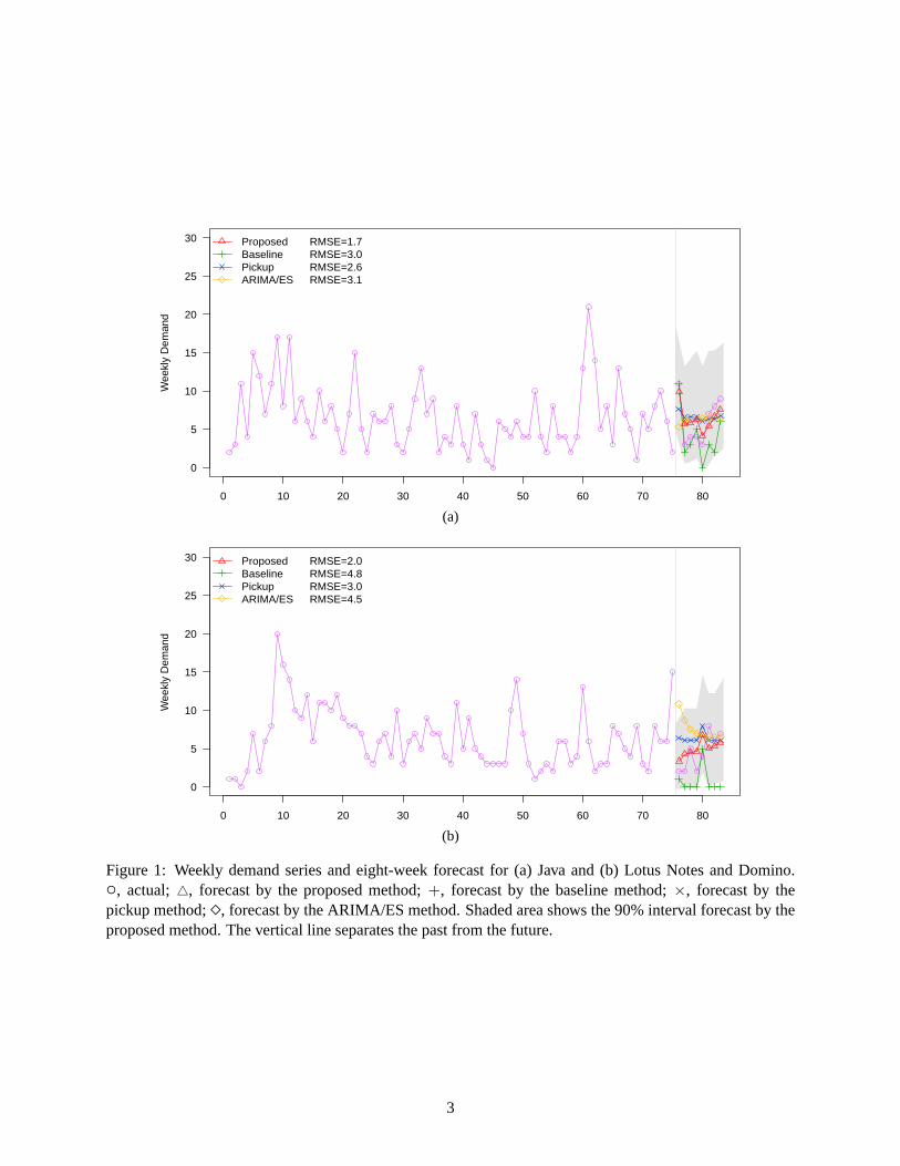
Demand of different skills can fluctuate dramatically over time in different ways. Figure 1 shows the

weekly time series of demand in two categories from a real-world resource pool operation which will be

discussed shortly. A conventional method of forecasting demand series such as these is to employ time

series models. Among the most popular ones are the autoregressive integrated moving-average (ARIMA)

models and the exponential smoothing (ES) models (Box, Jenkins, and Reinsel 2008). The forecasts shown

in Figure 1 with diamonds (⋄) are produced by the ARIMA/ES method using SPSS Expert Modeler, a

commercial-grade software package equipped with the desired capability ofautomatic data-driven model

selection — not only within the ARIMA family and the ES family respectively, but between them as well

(http://www-03.ibm.com/software/products/en/spss-forecasting).

In this article, we develop an alternative framework of demand forecasting. The basic idea is to leverage

the predictive information in a pipeline and combine the results with special complementary time series

models to produce the final forecast.

The pipeline in this context refers to the service provider’s event management system that facilitates

the creation and launch of work requests. The system mandates that every work item, before launched

for registration, goes through a sequence of preparation stages in an irreversible order of maturity as more

and more required information is provided by the client. The required information includes technological

requirements which dictate the skills needed for the work item. It also includes the so-called scheduled

start date which informs the system when to launch the work item for registration. Endowed with such

information, the work items contained in the pipeline at the time of forecasting, which we call theplanned

events, can be readily projected as future demand. In fact, these projections are often reported by the system

as demand outlook. We refer to this method of demand forecasting as the baseline method. It will be used to

normalize other methods when comparing their accuracies. In Figure 1, the forecasts by the baseline method

are shown with plus signs (+).

2

0 10 20 30 40 50 60 70 80

0

5

10

15

20

25

30

Wee

kly

Dem

and

ProposedBaselinePickupARIMA/ES

RMSE=1.7RMSE=3.0RMSE=2.6RMSE=3.1

(a)

0 10 20 30 40 50 60 70 80

0

5

10

15

20

25

30

Wee

kly

Dem

and

ProposedBaselinePickupARIMA/ES

RMSE=2.0RMSE=4.8RMSE=3.0RMSE=4.5

(b)

Figure 1: Weekly demand series and eight-week forecast for (a) Javaand (b) Lotus Notes and Domino.◦, actual;△, forecast by the proposed method;+, forecast by the baseline method;×, forecast by thepickup method;⋄, forecast by the ARIMA/ES method. Shaded area shows the 90% intervalforecast by theproposed method. The vertical line separates the past from the future.

3

In reservation-based service industries such as airlines and hotels, theso-called pickup method has been

successfully used for demand forecasting (L’Heureux 1986; Weatherford and Kimes 2003). In this method,

future demand is predicted by suitably scaling and shifting the total bookings on hand using historical

averages or regression techniques. The baseline forecast in our application is the counterpart of bookings on

hand and therefore can be used as input to a pickup model for demand forecasting. This method produces

the results shown in Figure 1 with crosses (×).

The planned events in the pipeline are subject to revisions. The scheduledstart date, in particular, can be

changed for various reasons and therefore is not a perfect indicator of the actual launch time. The discrep-

ancy between the scheduled start date and the actual launch time can be very large, ranging from days to

weeks, especially for work items in early stages of preparation when the information entered into the system

tends to be no more than a temporary place holder. To rely on the scheduled start date indiscriminately could

yield erroneous demand forecasts. Improving such forecasts by employing an advanced statistical method

to determine the actual launch time of planned events more reliably at any stage inthe pipeline constitutes

the first component of the proposed framework.

The pipeline at the time of forecasting does not contain any future work items that may contribute to

the demand at a forecasting horizon. For example, the work items created in the first week after the time

of forecasting may contribute to the demand in the second week. We call thesework items theunplanned

events. The unplanned events can take a bigger share in the total demand as the forecasting horizon in-

creases. It is especially the case when the system has no requirement onthe minimum lead time — the

time elapsed between the creation and the launch of a work item — as many work items may be created

on short notice. Predicting the contribution of unplanned events in the total demand at each forecasting

horizon to complement the demand predicted from the planned events constitutes the second component of

the proposed framework.

It is assumed in this article that demand forecasting takes place on a weekly basis and work items are

4

classified into predefined demand categories based on their technologicalrequirements. The objective of

demand forecasting is to predict the number of work items, or events, that willbe launched from each

demand category in each of the consecutive coming weeks (up to an upperbound). The time series shown

in Figure 1 represent such weekly demand from two categories and the corresponding eight-week forecasts

at the end of week 75.

Under the proposed framework, statistical survival functions for the lifetime of events in the pipeline

are employed to determine the actual launch time of planned events in forecasting their contribution to the

future demand. To complement the pipeline forecast, special time series models, including those for time

series of counts, are employed to predict the contribution of unplanned events to the total demand. The

results of this method are shown in Figure 1 with triangles (△).

Survival functions have been used as a forecasting tool in many applications. For example, Read (1997)

employs survival functions to forecast the attritions of U.S. Army personnel. Malm, Ljunggren, Bergstedt,

Pettersson, and Morrison (2012) use survival functions to forecast replacement needs for drinking water

networks. Canals-Cerda and Kerr (2014) discuss the use of survival functions to forecastcredit card portfolio

losses. The present application is served by a nonparametric hierarchical survival model that predicts the

remaining lifetimes of planned events in the pipeline. The hierarchy is constructed by taking advantage of

the personal behavior of event managers in scheduling the start date while overcoming the difficulty of data

disparity.

Time series models have been considered in Lee (1990) for predicting the daily bookings of a passen-

ger flight leading to the departure day. We employ time series models to predict the demand from un-

planned events to complement the demand from planned events predicted by the survival analysis method.

In addition to the ordinary (Gaussian) autoregressive models, we investigate the performance of linear and

log-linear Poisson autoregressive models which are specifically designed for time series of counts (Zeger

and Qaqish 1988; Fokianos and Tjøstheim 2011; Christou and Fokianos 2015). We also consider horizon-

5

specific autoregressive models which are tailored to the special horizon-dependent structure of the demand

from unplanned events in relation with the demand from planned events.

To develop and maintain a demand forecasting tool for operational use, theservice provider has some

choices to make on the spectrum of cost and complexity. The ARIMA/ES methodand the pickup method

are viable choices because they only require the collection and storage ofweekly demand series and the

straightforward application of existing software. To compete with them, the alternative method not only

needs to achieve higher accuracy but also has to keep its complexity within a suitable level.

The dataset that we use in this article to motivate and validate the proposed method is provided by a

multinational corporation that offers resource pool services for software development. It is a random sample

of the events they managed in two years. It is derived from a database ofweekly snapshots of the pipeline,

thus representing a discretized evolutionary history of each event overtime. Captured in the dataset are

two stages of event preparation, calledscheduled andscheduled-ready, with the latter representing greater

maturity, which are automatically designated to an event based on the informationprovided by the event

manager. There is also a preliminary draft stage which is ignored in our analysis because events in this stage

lack sufficient and reliable information for demand forecasting. Among the attributes associated with an

event in the dataset are the stage of preparation and the scheduled startdate and the required technologies.

These attributes are dynamic and subject to change during the course of evolution leading to the launch of the

event. Other useful attributes are the event identification number and the name of the event manager, which

do not change over time. Examples of required technologies areInfoSphere DataStage, Java, Lotus Notes

and Domino, andSAP. A single event may require one or more technologies. By means of a predefined

mapping, the required technologies determine the demand category of the event for the purposes of demand

forecasting. Figure 1 shows the weekly demand series in categories (a) Java and (b) Lotus Notes and

Domino. For reason of confidentiality, we will not divulge the complete list of technologies or the real scale

of demand in this article.

6

It is worth mentioning that information regarding the underlining project of each work item is not avail-

able in the dataset. This is not uncommon in resource pool services, especially for those run by third-party

providers, because such information is often considered internal and confidential by the client. More details

about the dataset will be given later during the analysis.

The remainder of this article is organized as follows. In Section 2, we discuss the prediction of demand

from planned events. In Section 3, we discuss the prediction of demand from unplanned events. In Section

4, we discuss the total demand forecast. Concluding remarks and discussions are given in Section 5.

2 Demand from Planned Events

At the time of forecasting, planned events are work items in the pipeline with adequate information including

the required technologies and the scheduled start date. Equipped with these attributes, it is a simple matter

of counting to determine how many planned events in a given demand categorywill be launched in a coming

week. For example, the total number of Java events with the scheduled startdate falling in the 2nd week

from the time of forecasting constitutes the demand for Java skills in that week.We call this method of

demand forecasting thebaseline method. So called because it is often implemented in the system to provide

a quick outlook of future demand, as is the case with the supplier of the dataset for the present study.

2.1 Survival Analysis Method

The baseline method has some serious shortcomings. For one, it relies solelyon the scheduled start date

to determine when a planned event will be launched. Unfortunately, the scheduled start date, entered into

the system by the event manager during the preparation stages, is not entirely reliable as an indicator of the

actual launch time, because the event could be rescheduled at any time (withno penalty) until it is actually

launched.

As an example, Figure 2 shows the histogram of the discrepancy between the scheduled start date and

7

−8 −7 −6 −5 −4 −3 −2 −1 0 1 2 3 4 5 6 7 8

Weeks Behind (−) or Ahead of (+) Scheduled Start Date

Eve

nt−

Wee

k (%

)

0

5

10

15

20

25

30

35

40

0

5

10

15

20

25

30

35

40

Figure 2: Histogram of discrepancy between scheduled start date and actual launch time. Negative valuemeans actual launch time is behind scheduled start date; positive value meansactual launch time is ahead ofscheduled start date.

the actual launch time of 272 events created by an event manager. In this case, the scheduled start date

incorrectly predicts the actual launch time for nearly 60% of the event weeks (an event week is defined as

an event spending one week in the pipeline). The discrepancy can be very large: some events are postponed

by as much as 8 weeks and some others are advanced by as much as 6 weeks. Due to the prevalence of such

errors, relying on the scheduled start date for demand forecasting often produces poor results.

An event stays in the pipeline for a certain amount of time until it is launched. The actual launch time

of a planned event can be formulated as the remaining lifetime of the event in thepipeline. Therefore, it is

quite natural to model the entire lifetime of an event in the pipeline as a random variable to account for its

uncertainty, and employ survival functions to describe the actual launchtime in probabilistic terms.

To be more specific, letW denote the total number of weeks, measured in accordance with the weekly

snapshot schedules, that an event spends in the pipeline before it is launched. RegardingW as an integer-

valued nonnegative random variable, the survival function ofW is defined by

S(τ) := Pr(W > τ) (0≤ τ < ∞).

8

For a planned event that has been in the pipeline fora weeks at the time of forecasting, the probability that

the event will be launched in the coming weekh is given by

p(h|a) := Pr(W = a+h−1|W ≥ a) =S(a+h−2)−S(a+h−1)

S(a−1)(h = 1,2, . . .). (1)

The functionp(·|a) is nothing but the probability mass function of an integer-valued positive random vari-

able that represents the week in which the event will be launched. It can be regarded as a probabilistic

prediction of the launch time over the coming weeks. It is interesting to observethat

p(h|a) = {1−λ (a)}{1−λ (a+1)}· · ·{1−λ (a+h−2)}λ (a+h−1),

whereλ (a) := {S(a−1)−S(a)}/S(a−1) = p(1|a) is called the hazard rate at the age ofa.

Suppose the pipeline containsn planned events in weekt, which is the time of forecasting. Letci denote

the demand category of eventi (i = 1, . . . ,n), Si(·) andai denote the survival function and the age of eventi,

and pi(·|ai) denote the corresponding prediction function for the launch time of eventi. Then, the number

of planned events that will be launched in weekt +h as demand in categoryc, denoted byD(t +h|t,c), can

be modeled as

D(t +h|t,c) =n

∑i=1

Bi(h,c), (2)

whereB1(h,c), . . . ,Bn(h,c) are Bernoulli random variables with success probability given by

φi(h,c) := pi(h|ai)I(ci = c). (3)

9

The expected value ofD(t +h|t,c) in (2) takes the form

π(t +h|t,c) := E{D(t +h|t,c)}=n

∑i=1

φi(h,c). (4)

This constitutes the best point forecast for the number of planned eventsin categoryc to be launched in

weekt +h based on the minimum mean-square error (MMSE) criterion.

If the events are launched independently, then the variance ofD(t +h|t,c) can be expressed as

σ2π (t +h|t,c) :=V{D(t +h|t,c)}=

n

∑i=1

φi(h,c){1−φi(h,c)}. (5)

The independence assumption also implies thatD(t +h|t,c) has a Poisson binomial distribution from which

an interval forecast can be easily derived. Incorporating dependencies in the model is expected to improve

the accuracy of interval forecast and variance calculation, although the point forecast will not be affected.

Finally, we employ an allocation method to accommodate possible misclassification of events in (4). Let

ri(c,c′) denote the probability of eventi being misclassified in categoryc′ instead ofc. Then, the modified

success probability ofBi(h,c) is given by

φi(h,c) := pi(h|ai)ri(c,ci). (6)

In practice, the allocation parametersri(c,c′) can be derived from historical data at suitably aggregated

levels such as the preparation stage and the age of the event.

The survival analysis method relies solely on the observed lifetimes of events to determine the launch

time. This does not mean that the scheduled start date, which feeds the baseline method, should be com-

pletely ignored. In general, the scheduled start date is noisy, but the amount of noise can vary among demand

categories, for example. In the cases where the scheduled start date has little noise, the baseline forecast

10

can be more accurate than the survival-based forecast. The opposite isgenerally true where the scheduled

start date has too much noise. The question is how to combine these forecastsappropriately to produce

better results. Toward that end, we develop two hybrid methods by incorporating the scheduled start date at

different levels: the event level and the demand category level.

The first hybrid method identifies the so-called trusted event managers by the criterion that the events

they manage are launched mostly according to the scheduled start date. Foreach event of a trusted event

manager, the survival-based prediction of launch time is replaced by the scheduled start date of the event.

The second hybrid method combines the baseline forecast, denoted byπB(t +h|t,c), with the survival-

based forecast or the forecast by the first hybrid method, both denoted by πS(t + h|t,c) for simplicity. The

resulting forecast takes the form

πR(t +h|t,c) := α(h,c)πS(t +h|t,c)+β (h,c)πB(t +h|t,c), (7)

where the coefficientsα(h,c) andβ (h,c) are derived from historical data by least-squares regression. Note

that the coefficients are allowed to vary withh in order to accommodate the situation where the benefit of

the baseline forecast depends on the forecasting horizon.

The hybrid method in (7) is interpretable as a generalization of a Bayesian estimator. Indeed, the baseline

forecastπB(t +h|t,c) can be expressed in the form of (4) withφi(h,c) replaced byBi0(h,c), which equals 1

if eventi is in categoryc and the scheduled start date falls in weekh, and equals 0 otherwise. Therefore, the

regression model (7) can be rewritten as

πR(t +h|t,c) =n

∑i=1

{α(h,c)φi(h,c)+β (h,c)Bi0(h,c)}.

If the coefficients are constrained to take nonnegative values and sum up to 1, then the termα(h,c)φi(h,c)+

β (h,c)Bi0(h,c) can be interpreted as the Bayesian MMSE estimator (i.e., the posterior mean) ofthe Bernoulli

11

random variableBi(h,c) given the binary observationBi0(h,c), with the survival-based forecastφi(h,c) serv-

ing as the mean of a Beta prior.

The allocation method in (6) can also be improved by incorporating the concept of trusted event man-

agers. In this case, the trusted event managers are identified by sufficiently high rates of no change to the

demand category for the events they manage. Exemption from allocation is granted to all events managed

by trusted event managers. This can be done by settingri(c,c′) = 0 in (6) for c′ 6= c if event i of categoryc′

qualifies for the exemption.

2.2 Survival Function Modeling

To implement the survival analysis method in practice, one needs to designatea survival function for each

event in the pipeline. Survival functions can be derived from historical data by statistical techniques. The

simplest model is to apply a grand survival function to all events. However, a stratified approach based on

a suitable segmentation of the event population is more appropriate to accommodate the expected heteroge-

neous characteristics of the events.

Because the event managers are responsible for creating and scheduling events in the pipeline, their

individual behavior, dictated by personal preferences and the dynamics of underlying projects, should have

a direct impact on the lifetime of the events they manage. It is desirable that the event population be

segmented by event manager so that a personalized survival model canbe developed. In practice, this idea

runs immediately into the obstacle of data disparity: segmentation by event manager inevitably leads to a

small number of segments with sufficient data points and a large number of segments with few data points.

Training an exclusive survival function for each segment is likely to result in unreliable models with poor

predictive capability due to their excessive statistical uncertainty.

As a practical starting point, we present a hierarchical approach to tackle the problem (see Section 5

for comments on alternative methods). The approach yields a class-basedmodel where some personalized

12

Figure 3: An example of hierarchical survival models with 2 tier-1 classesand 5 tier-2 classes plus a sup-plementary class for the remaining event segments.

segments retain their own survival functions whereas the others share common survival functions in the

hierarchy.

Specifically, we consider a hierarchy with two tiers of event classes as illustrated by Figure 3. Tier-1

classes are defined by selected demand categories. This is a natural choice because demand forecasting is

carried out at the granularity of demand categories. Tier-2 classes aredefined by selected event managers

under each selected demand category, representing a personalized refinement of the tier-1 parent classes.

The hierarchy of event classes enables a hierarchical approach to designation of survival functions for

planned events in demand forecasting: First, determine whether or not a given event belongs to a tier-2

class; if yes, use the survival function associated with the tier-2 class; otherwise, determine whether or not

the event belongs to a tier-1 class; if yes, use the survival function associated with the tier-1 class; if both

tests fail, use the survival function associated with the supplementary class. In other words, the survival

function designated to a planned event for demand forecasting is one associated with the class in the deepest

tier to which the event belongs.

Searching for the best classes over all possible subsets of event segments is prohibitively time-consuming.

To circumvent the difficulty, we consider a sequential (suboptimal) selectionprocedure, such that the can-

didate segments are admitted into a given tier one after another, in descendingorder of sample size, until

the out-of-sample predictive power of the resulting survival model is maximized. For tier-1 classes, the pro-

13

cedure is applied to the segments defined by demand category, and the unselected segments form a single

supplementary class. For tier-2 classes, the procedure is applied to the segments defined by event manager

under each demand category admitted into tier 1.

An alternative procedure is what we call forward selection. It is analogous to the forward selection

procedure of stepwise regression, except that the criterion for enteris based on the out-of-sample predictive

power rather than a significance test. In each iteration, the forward selection procedure picks the best

segment from the pool of remaining candidates until the out-of-sample predictive power is maximized. It

is more effective than sequential selection, but the computational complexity isconsiderably higher, as the

number of trials increases quadratically rather than linearly with the number ofcandidates.

The out-of-sample predictive power is an appropriate criterion for survival modeling in the present

application because demand forecasting is its ultimate objective. Specifically, we determine the out-of-

sample predictive power byK-fold cross validation: The entire dataset is partitioned randomly intoK equal-

sized subsets. A survival model is trained in turn on theK −1 out ofK subsets and tested on the remaining

one using a prediction error metric. This generatesK out-of-sample error measurements whose average

serves as the modeling criterion.

A useful prediction error metric is what we call theQ-score, which measures the relative improvement

by a method of interest over the baseline method in root mean-square error(RMSE) for forecasting the

demand from planned events. Specifically, theQ-score is defined as

Q := 1−RMSE(method of interest)RMSE(baseline method)

. (8)

This metric can be calculated using the RMSE for a given demand category ata given forecasting horizon to

obtain a category-and-horizon-specificQ-score. It can also be calculated using the average of the RMSE’s

across demand categories and forecasting horizons to produce an overall Q-score. Maximizing the overall

14

Q-score obtained from cross validation is the criterion of the sequential andforward selection procedures.

Finally, for greater versatility, we take the preparation stage into account insurvival modeling. Owing to

the irreversible order of maturity, events in a later stage tends to have less uncertainty regarding the lifetime

than events in an earlier stage. A stage-dependent survival model is expected to provide more accurate

demand forecast. The survival analysis method discussed above can be applied independently to each stage.

The resulting stage-dependent survival functions describe the stage-specific lifetime—the time elapsed after

an event enters the said stage until it is launched. When forecasting the demand, these functions are used to

determine the launch time of planned events in a stage conditional on the time spentin that stage.

Given the hierarchy of event classes, the corresponding survivalfunctions can be derived from historical

data using any number of statistical techniques (Lawless 2002; Kalbfleischand Prentice 2002). A key

requirement is the ability to accommodate right-censored events—the events that are still under preparation

at the time of final snapshot. An important example of such techniques is the product-limit estimator, also

known as the Kaplan-Meier estimator (Kaplan and Meier 1958). Being fully nonparametric, the Kaplan-

Meier estimator has the utmost flexibility for fitting a wide variety of observed survival patterns without

strong assumptions. This property is particularly desirable for large-scale modeling exercises such as ours

where fine-tuning of each and every survival function with elaborate models is prohibitive.

Let τ1 < · · · < τm be the distinct lifetimes of historical events in the class of interest. Forj = 1, . . . ,m,

let r j denote the number of events in the said class with lifetime or censoring time greaterthan or equal to

τ j, and letd j denote the number events in the said class with lifetime equal toτ j. Then, the Kaplan-Meier

estimator of the survival functionS(τ), with τ being a continuous variable, can be expressed as

S(τ) := ∏j:τ j≤τ

(1−d j/r j) (0≤ τ < ∞). (9)

This formula defines a right-continuous and monotone-decreasing step function, starting withS(0) = 1. For

15

the weekly snapshot data, a drop in this function can only take place at positive integersτ = 1,2, . . . , and

the magnitude of the drop atτ represents the probability that an event spendsτ weeks in the pipeline before

it is launched in the following week.

The Kaplan-Meier estimator is not without limitations. For example, it tends to exhibit higher statistical

variability in the right-hand tail where observations are sparse; it is also unable to extrapolate the survival

function beyond the largest observation (except for setting it to zero).These shortcomings can have a

negative impact on demand forecasting especially for events in advancedage. To mitigate the problem, one

can model the lifetimes jointly across event classes under the semi-parametric Cox proportional hazards

(PH) framework (Cox and Oakes 1984).

For example, consider a joint model of all survival functions in the two-tiered hierarchy. LetIu be the

event membership indicator for tier-1 classu and letIuv be that for tier-2 classv under tier-1 classu. Then,

the Cox proportional hazards model can be expressed as

log{S(τ)}= log{S0(τ)}exp

{ k

∑u=1

αuIu +k

∑u=1

ku

∑v=1

βuvIuv

}

, (10)

whereS0(·) is a nonparametric baseline survival function,αu andβuv are the parameters which adjust the

baseline survival function for different event classes,k is the number of tier-1 classes (minus 1 if the supple-

mentary class is absent), andku is the number of tier-2 classes under tier-1 classu (minus 1 if it equals the

number of segments under tier-1 classu).

Leveraging the data across all event classes allows the Cox estimator to overcome the aforementioned

shortcomings of the Kaplan-Meier estimator. However, the assumption of proportional hazards imposes a

limitation on its flexibility. Less restrictive models can be developed by considering each tier separately,

resulting in a model of the form (10) without theβuv terms for tier 1 and a similar model without theαu

terms for tier 2.

16

2.3 Case Study

The dataset discussed in Section 1 contains the weekly evolution history of 6,747 events in 126 demand

categories. There are 6,278 events with records in stage 1 (scheduled)and 2,301 events with records in

stage 2 (scheduled-ready). The fact that not all events have records in both stages is due to the limitation

of the weekly sampling resolution. It is more pronounced for stage 2 because the sojourn times tend to be

shorter in that stage. In survival modeling, the RMSE is calculated on the basis of weekly forecasts over 99

consecutive weeks for the number of planned events in each demand category that are launched in the next

1 through 8 weeks.

In this study, the allocation method defined by (6) is always applied to the survival-based forecasts. The

trusted event managers are identified, separately for each stage, as one who manages at least 5 events and

makes no revisions to the demand category. Their events are exempted fromallocation. The remaining

events are used to derive the fractions of event misclassification in each stage that serve as stage-dependent

allocation parameters.

A 10-fold cross-validation method is used to calculate the out-of-sampleQ-score as the criterion for

construction of the two-tiered hierarchy. Tier-1 classes are obtained first, by using a one-tiered forecasting

approach without requiring tier-2 classes. This step is carried out separately for each preparation stage.

After tier-1 classes are determined, tier-2 classes are selected by using the two-tiered forecasting approach

with fixed tier-1 classes.

As candidates for tier-1 classes, the event segments defined by demand category exhibit a great disparity

in size. For stage-1 events, for example, the size ranges from 1 to 492 witha median of 25, indicating a very

skewed distribution. The sequential selection procedure yields a survival model with 15 classes for stage-1

events and 8 classes for stage-2 events.

Figure 4 shows the survival functions by the Kaplan-Meier estimator in (9), obtained using the R function

survfit, for two of the resulting tier-1 classes of stage-1 events. Figure 4 also shows the corresponding

17

probability distributions of launch time, given by (1), for events of age 1, i.e., p(h|1) (h = 1,2, . . .). As can

be seen, these event classes have distinct characteristics in launch time. For example, the launch time of Java

events is most likely to fall into week 1 with roughly equal chances over the remaining weeks, whereas the

launch time of SAP events is more likely to occur around week 5 or 6 with little chance of staying beyond

week 10.

For comparison, Figure 4 also depicts the survival functions by the Cox proportional hazards estimator

of the form (10) without the tier-2 terms, which are obtained using the R function coxph. This result

demonstrates the Cox estimator’s ability to extrapolate beyond the largest observation, which is desirable

especially for the SAP events. However, the Cox estimator does not fit the observed lifetimes of SAP events

very well, due to the restriction of proportional hazards.

The candidates for tier-2 classes are even more unbalanced in size. Among the 1,279 segments of stage-1

events, the size ranges from 1 to 199 with a median equal to 2. The sequential selection procedure produces

92 tier-2 classes for stage-1 events and 6 for stage-2 events. The tier-2 classes constitute a personalized

refinement of their parent classes in tier 1. For example, the Java class in tier 1 is further refined by 11 tier-2

classes, and the SAP class by 2, all corresponding to different eventmanagers. Figure 5 depicts the survival

functions of four tier-2 classes for Java events together with the survival function of the parent class. The

admission of these tier-2 classes in the hierarchy is justified by their unique survival patterns.

To evaluate the predictive power of the survival analysis method, Table 1contains the out-of-sampleQ-

score (in percentage) for three survival models: one which employs a grand survival function for all events

(the no-tier model), one which employs tier-1 classes only (the one-tier model), and one which makes full

use of the two-tiered hierarchy (the two-tier model). All survival functions are produced by the Kaplan-

Meier estimator. The results show that the out-of-sample performance improves with the complexity of the

survival model, and the personalized two-tier model achieves the highestaccuracy.

It is worth pointing out the Cox proportional hazards method produces inferior results. For example,

18

0 5 10 15 20 25 30 35 40 45 50 55 60 65 70 75 80

0.0

0.1

0.2

0.3

0.4

0.5

0.6

0.7

0.8

0.9

1.0

Weeks

Sur

viva

l Pro

babi

lity

Kaplan−MeierCox PH

0 5 10 15 20 25 30 35 40 45 50 55 60 65 70 75 80

0.0

0.1

0.2

0.3

0.4

0.5

0.6

0.7

0.8

0.9

1.0

Weeks

Sur

viva

l Pro

babi

lity

Kaplan−MeierCox PH

(a) (b)

1 2 3 4 5 6 7 8 9 10 11 12 13

0.00

0.02

0.04

0.06

0.08

0.10

0.12

0.14

0.16

0.18

0.20

Future Week

Pro

babi

lity

0.00

0.02

0.04

0.06

0.08

0.10

0.12

0.14

0.16

0.18

0.20

1 2 3 4 5 6 7 8 9 10 11 12 13

0.00

0.02

0.04

0.06

0.08

0.10

0.12

0.14

0.16

0.18

0.20

Future Week

Pro

babi

lity

0.00

0.02

0.04

0.06

0.08

0.10

0.12

0.14

0.16

0.18

0.20

(c) (d)

Figure 4: (a)(b) Survival functions for two tier-1 classes, by the Kaplan-Meier estimator (solid line) and theCox proportional hazards estimator (dashed line), and (c)(d) the corresponding probabilities of launch timeover the next thirteen weeks for events of age 1, by the Kaplan-Meier estimator. (a)(c) Java events. (b)(d)SAP events. Shaded area in (a)(b) shows the 95% confidence band ofthe Kaplan-Meier estimates.

19

0 5 10 15 20 25 30 35 40 45 50 55 60 65 70 75 80

0.0

0.1

0.2

0.3

0.4

0.5

0.6

0.7

0.8

0.9

1.0

Weeks

Sur

viva

l Pro

babi

lity

Parent Class

Figure 5: Survival functions of four tier-2 classes and their parent class for Java events.

Table 1: Performance for Forecasting Demand from Planned EventsEvent Class Survival Analysis Models Hybrid Models

Selection Method No-Tier One-Tier Two-Tier Trusted Mgr. Regression BothSequential Selection 15.42 16.00 16.60 19.80 22.84 23.82Forward Selection 15.42 16.16 17.42 20.59 23.47 24.38

Note: Results are based on 10-fold cross validation.

applying the Cox estimator independently to each tier and preparation stage yields an out-of-sampleQ-

score of 15.59% as compared to 16.60% achieved by the Kaplan-Meier estimator. This suggests that the

potential benefit of the Cox estimator is not sufficiently fulfilled to compensate for its shortcomings. It

remains to be seen if the outcome can be improved by further stratification of each tier to maximize the

benefit of the proportional hazards constraint.

To evaluate the performance of the hybrid methods that incorporate the scheduled start date with the

survival-based forecasts, Table 1 contains the out-of-sampleQ-score for three variations of the methods:

one which replies only on the trusted event managers, one which employs theregression model, and one

which uses both methods. The trusted event managers are those with a history of at least 5 event-weeks in

the training data and 80% or higher on-time rate for launching their events. Allvariations are built upon the

forecasts of the two-tiered survival model. The results show that the regression method is more effective

20

between the two, but applying both methods together achieves the highest accuracy.

For comparison, an hierarchy of event classes is also obtained using theforward selection procedure. It

comprises 17 tier-1 classes for stage-1 events and 5 for stage-2 events; it also comprises 51 tier-2 classes for

stage-1 events and 1 tier-2 class for stage-2 events. Table 1 shows the resultingQ-scores. As compared with

the sequential selection procedure, the forward selection procedure offers higher accuracy with a smaller

number of classes in the hierarchy, an indication of greater efficiency. However, this is achieved at a much

higher computational cost (e.g., days instead hours). The sequential selection procedure suffers slightly in

accuracy, but it requires much less time to compute and therefore qualifies as a practical choice.

Finally, let us examine the effect of the survival analysis method more closely at the granularity of de-

mand categories and forecasting horizons. Figure 6 depicts theQ-scores of four models at eight forecasting

horizons for six demand categories. The results are based on in-sample RMSE’s with the survival functions

and the hybrid models trained on the entire dataset.

As can be seen from Figure 6(a), the one-tiered survival model is ableto improve the baseline method

in all but one cases, the only exception being week 1 of category 6 (Cognos). TheQ-score varies from

−1% to 74%, depending on the demand category and the forecasting horizon. For some demand categories,

such as category 5 (SAP), the forecast in shorter terms tends to benefitmore from the survival analysis

method than the forecast in longer terms; the opposite is true for some other categories, such as category

6 (Cognos). Figure 6(b) shows the correspondingQ-scores of the two-tiered survival model that employs

personalized event classes. Better results are obtained in 45 out of the 48 cases. The most noticeable ones

include category 2 (Infosphere DataStage) and category 4 (SQL) at all horizons.

Figure 6(c) depicts theQ-scores of the hybrid method which uses the trusted event managers to revise

the forecasts of the two-tiered survival model. In 30 out of the 48 cases, the hybrid model produces better

results than the original two-tiered survival model. An example is week 1 of category 3 (Lotus Notes and

Domino). Finally, Figure 6(d) shows theQ-scores of the hybrid method that employs both trusted event

21

1 2 3 4 5 6

Demand Category

Q−

Sco

re (

%)

0

10

20

30

40

50

60

70

80

90

0

10

20

30

40

50

60

70

80

90Week 1Week 2Week 3Week 4Week 5Week 6Week 7Week 8

1 2 3 4 5 6

Demand Category

Q−

Sco

re (

%)

0

10

20

30

40

50

60

70

80

90

0

10

20

30

40

50

60

70

80

90Week 1Week 2Week 3Week 4Week 5Week 6Week 7Week 8

(a) (b)

1 2 3 4 5 6

0

10

20

30

40

50

60

70

80

90

Demand Category

Q−

Sco

re (

%)

0

10

20

30

40

50

60

70

80

90Week 1Week 2Week 3Week 4Week 5Week 6Week 7Week 8

1 2 3 4 5 6

0

10

20

30

40

50

60

70

80

90

Demand Category

Q−

Sco

re (

%)

0

10

20

30

40

50

60

70

80

90Week 1Week 2Week 3Week 4Week 5Week 6Week 7Week 8

(c) (d)

Figure 6: TheQ-scores of four models for forecasting demand from planned events in six categories at eighthorizons. (a) One-tiered survival model. (b) Two-tiered survival model. (c) Hybrid model using trustedevent managers. (d) Hybrid model using trusted event managers and regression. Demand categories are: (1)Java, (2) Infosphere DataStage, (3) Lotus Notes and Domino, (4) SQL, (5) SAP, and (6) Cognos.

22

managers and regression. This method produces the best results, with theQ-scores ranging from 16% to

77%. It is also the only model that performs better than the baseline method forweek 1 of category 6

(Cognos).

Table 2 shows the detailed regression models for two demand categories: Java and Infosphere DataStage.

The models are presented in a reparameterized form rather than the original form (7) in order to perform

the T -test for the statistical significance of the additional contributions from the baseline forecast and the

interactions with the forecasting horizon. The last column contains thep-values of theT -test under the i.i.d.

Gaussian assumption.

As the main effect, the significance of the survival-based forecast is evident in both models. The addi-

tional contribution from the baseline forecast is quite significant in the Javamodel but much less so in the

Infosphere DataStage model. The forecasting horizon plays an importantrole in the Infosphere DataStage

model through the interaction with the survival-based forecast. This result lends support to the horizon-

dependent modeling approach in (7).

3 Demand from Unplanned Events

Unplanned events are the future events that arrive at the pipeline after the time of forecasting and before the

targeted forecasting horizon. As shown in Figure 7, the unplanned events can contribute significantly to the

total demand, and their share increases with the forecasting horizon.

3.1 Time Series Method

By dropping the demand category in notation for simplicity, letD(t +h|t) denote the demand in weekt +h

which is generated from the planned events at the end of weekt. Then, the total demand in weekt + h,

23

Table 2. Regression Models for Two Demand CategoriesJava

Parameter Estimate Std. Error T -Value Pr(> |T |)Survival Forecast 0.633 0.102 6.224 0.000

Survival Forecast:Horizon2 -0.021 0.172 -0.125 0.901Survival Forecast:Horizon3 0.003 0.183 0.014 0.989Survival Forecast:Horizon4 -0.025 0.172 -0.143 0.886Survival Forecast:Horizon5 -0.001 0.186 -0.004 0.997Survival Forecast:Horizon6 -0.075 0.198 -0.377 0.706Survival Forecast:Horizon7 -0.126 0.191 -0.659 0.510Survival Forecast:Horizon8 -0.090 0.212 -0.425 0.671

Baseline Forecast:Horizon1 0.102 0.057 1.789 0.074Baseline Forecast:Horizon2 0.241 0.074 3.267 0.001Baseline Forecast:Horizon3 0.229 0.081 2.816 0.005Baseline Forecast:Horizon4 0.261 0.073 3.579 0.000Baseline Forecast:Horizon5 0.196 0.078 2.511 0.012Baseline Forecast:Horizon6 0.221 0.080 2.755 0.006Baseline Forecast:Horizon7 0.258 0.074 3.499 0.000Baseline Forecast:Horizon8 0.242 0.086 2.810 0.005

Infosphere DataStageParameter Estimate Std. Error T -Value Pr(> |T |)

Survival Forecast 0.629 0.078 8.037 0.000

Survival Forecast:Horizon2 0.220 0.112 1.958 0.051Survival Forecast:Horizon3 0.399 0.112 3.551 0.000Survival Forecast:Horizon4 0.443 0.111 4.004 0.000Survival Forecast:Horizon5 0.482 0.114 4.217 0.000Survival Forecast:Horizon6 0.344 0.120 2.857 0.004Survival Forecast:Horizon7 0.351 0.128 2.741 0.006Survival Forecast:Horizon8 0.337 0.132 2.557 0.011

Baseline Forecast:Horizon1 0.190 0.051 3.735 0.000Baseline Forecast:Horizon2 0.076 0.056 1.359 0.175Baseline Forecast:Horizon3 -0.089 0.055 -1.605 0.109Baseline Forecast:Horizon4 -0.095 0.057 -1.674 0.095Baseline Forecast:Horizon5 -0.145 0.062 -2.328 0.020Baseline Forecast:Horizon6 -0.028 0.072 -0.389 0.697Baseline Forecast:Horizon7 0.001 0.080 0.015 0.988Baseline Forecast:Horizon8 -0.026 0.085 -0.307 0.759

24

1 2 3 4 5 6 7 8

Horizon

Sha

re o

f Unp

lann

ed E

vent

s (%

)

0

10

20

30

40

50

60

70

80

90

100

0

10

20

30

40

50

60

70

80

90

100

Figure 7: Average proportion of unplanned events in weekly total demandat different forecasting horizonsfor the dataset discussed in Section 1.

denoted byγ(t +h), can be written as

γ(t +h) = D(t +h|t)+δ0(t +h)+δ1(t +h)+ · · ·+δh−1(t +h). (11)

In this expression, theδk(t+h) (k = 0,1, . . . ,h−1) denote the number of events that are created in the future

weekt +h− k and launched in weekt +h at agek. We call these terms the demand from unplanned events.

Note that the events launched in weekt +h at ageh or older are accounted for inD(t +h|t) as the demand

from planned events.

To predict the demand from unplanned events, one can work directly with the time series

∆h(t) :=h−1

∑k=0

δk(t) (t = h,h+1, . . .), (12)

which represents the weekly totals of events launched at an age less thanh. Let ∆h(t + h|t) denote the

h-step ahead forecast of∆h(t + h) at timet by a suitable time series model based on the observed values

∆h(t),∆h(t −1), . . . ,∆h(h). Let π(t +h|t) denote the forecast ofD(t +h|t) by the survival analysis method.

25

Figure 8: Composition of total demand and its prediction by planned and unplanned events.

Then, by virtue of (11) and (12), the total demandγ(t +h) can be predicted by

γ(t +h|t) := π(t +h|t)+∆h(t +h|t). (13)

The composition of the total demand and its prediction is illustrated by Figure 8.

As shown in Figure 8, the forecasting of total demand at multiple horizons entails a unique requirement

for the prediction of multiple time series: In order to obtain the forecasts of totaldemand ath = 1, . . . ,h0

with some predetermined maximum horizonh0 > 1, one is required to predict each of the time series

{∆1(t)}, . . . ,{∆h0(t)} at a single but different horizon. Specifically, anh-step ahead prediction is needed

for series{∆h(t)} (h = 1, . . . ,h0), rather than multiple predictions at all horizons for all series.

3.2 Time Series Modeling

Linear prediction is a widely-used technique for time series forecasting (Box, Jenkins, and Reinsel 2008). A

simple method is autoregression, where the future value of a time series is predicted by a linear combination

of past observations. More specifically, thek-step ahead prediction of∆h(t+k) at timet is given recursively

26

by

∆h(t + k|t) = a0+p

∑i=1

ai ∆h(t + k− i|t) (k = 1,2. . . ,h), (14)

where∆h(t + k− i|t) := ∆h(t + k− i) for i ≥ k. The MMSE optimality of the predictor in (14) requires the

assumption of an autoregressive (AR) model of the form

∆h(t +1) = a0+p

∑i=1

ai ∆h(t +1− i)+ ε(t), (15)

where{ε(t)} is Gaussian white noise with mean zero and some varianceσ2. The coefficientsa0,a1, . . . ,ap

can be derived from historical data by several methods, including the Yule-Walker method and the least-

squares method. The orderp can be determined by data-driven criteria such as Akaike’s information crite-

rion (AIC) or the Bayesian information criterion (BIC).

In essence, the autoregressive model in (15) assumes that the conditional distribution of the random

variable∆h(t+1), given historical information up to timet, which we denote byFt , is independent Gaussian

with meana0+∑pi=1 ai ∆h(t +1− i) and varianceσ2. Because the time series in our problem consists of

nonnegative integer-valued counts, the Gaussian assumption is not satisfied. In particular, the symmetrical

property of the Gaussian distribution about the mean is an ill fit to the time series of counts with positively

skewed distributions. As a consequence, the predictor (14) may yield negative values that need to be replaced

by zero in order to conform with the nonnegative property of the data. Toovercome this deficiency, we

consider some alternative methods which are developed by substituting the Gaussian distribution with an

integer-valued probability model (e.g., Zeger and Qaqish 1988; Christou and Fokianos 2015).

The most popular example is the Poisson model where it is assumed that∆h(t +1), conditional onFt ,

27

has an independent Poisson distribution with certain meanλ (Ft), i.e.,

Pr{∆h(t +1) = d|Ft}=λ (Ft)

d

d!exp{−λ (Ft)} (d = 0,1, . . .).

As in the Gaussian case, the meanλ (Ft) can be modeled as a linear combination of past observations of the

time series such that

λ (Ft) := a0+p

∑i=1

ai ∆h(t +1− i). (16)

The coefficients can be derived from historical data under the framework of generalized linear models

(GLM). However, unlike the Gaussian case, the meanλ (Ft) must be positive in the Poisson model. It is

easy to see that the positivity constraint requires the coefficients to satisfya0 > 0 andai ≥ 0 for i = 1, . . . , p.

Furthermore, it is desirable that the model should lead to a stable time series with constant meanµ > 0. By

virtue of (16),µ must be the solution to the equationµ = a0+∑pi=1 aiµ, so the stability constraint requires

∑pi=1 ai < 1. This condition also ensures the second-order stationarity of the time series (Ferland, Latour, and

Oraichi 2006). Because of these constraints, the computational complexityof training the Poisson model is

much higher than the Gaussian model.

An alternative way of specifying the meanλ (Ft) is through a log transform such that

log{λ (Ft)} := a0+p

∑i=1

ai log(∆k(t +1− i)+1). (17)

Unlike the linear model in (16) where the past observations have an additive effect on the mean, the log-

linear model in (17) assumes an multiplicative effect,

λ (Ft) = exp(a0)p

∏i=1

(∆k(t +1− i)+1)ai .

28

An advantage of the latter is that the coefficients can be derived under theGLM framework without the

need of additional positivity constraint. However, a certain stability constraint is still desirable, although the

exact form of such constraint remains unknown except for the special case ofp = 1 which requires|a1|< 1

(Fokianos and Tjøstheim 2011).

For these time series models, the one-step ahead prediction∆h(t +1|t) := E{∆h(t +1)|Ft} can be easily

obtained because it is equal toλ (Ft) by definition. Under the linear model (16), the recursive algorithm in

(14) remains valid for computing thek-step ahead prediction∆h(t +k|t) := E{∆h(t +k)|Ft} with k ≥ 2. For

example, by the law of iterated expectations, we have

∆h(t +2|t) := E{∆h(t +2)|Ft}

= E{E[∆h(t +2)|Ft+1]|Ft}

= E{λ (Ft+1)|Ft}

= E

{

a0+p

∑i=1

ai ∆h(t +2− i)

∣

∣

∣

∣

Ft

}

= a0+p

∑i=1

ai ∆h(t +2− i|t).

In this algorithm, future values of the time series are simply substituted by the predicted values as the

recursion progresses fromt +1 to t +2 based on (16). In the Gaussian case, all negative predictions are set

to zero at the end of the recursion.

For the log-linear model (17), the substitution method becomes invalid in the recursive algorithm. For

example, it is easy to show that

∆h(t +2|t) = E

{

exp

[

a0+p

∑i=1

ai log(∆h(t +2− i)+1)

]∣

∣

∣

∣

Ft

}

6= exp

[

a0+p

∑i=1

ai log(∆h(t +2− i|t)+1)

]

.

29

A practical way of computing the predicted value∆h(t + k|t) for k ≥ 2 is Monte Carlo simulation. More

specifically, the predicted value∆h(t + k|t) is approximated by the average ofm independent samples (for

suitably largem). Theℓ-th sample, denoted by∆(ℓ)h (t+k|t), is drawn randomly from the Poisson distribution

with mean

exp

{

a0+p

∑i=1

ai log(∆(ℓ)h (t + k− i|t)+1)

}

(ℓ= 1, . . . ,m), (18)

and the initial values are given by∆(ℓ)h (t+k− i|t) := ∆h(t+k− i) if i≥ k. Note that the mean in (18) employs

simulated samples from previous recursions where actual values are notavailable.

Finally, let us discuss a different kind of time series models which are tailoredto the special structure of

the demand from unplanned events. According to (13), it is only theh-step ahead prediction that is needed

for series{∆h(t)} in order to obtain the forecast of the total demand at horizonh. The time series models

discussed before produce theh-step ahead prediction through a recursion which generates intermediate

predictions from step 1 to steph−1 before arriving at the final prediction in steph. We call them recursive

models of prediction. An alternative approach is to employ a linear function ofpast observations in the form

of (16) to model directly theh-step ahead conditional mean rather than the one-step ahead conditional mean.

In other words, it is assumed that∆h(t +h), rather than∆h(t +1), has a conditionally independent Gaussian

or Poisson distribution with mean

λ (Ft) := E{∆h(t +h)|Ft},

which takes the linear form (16). In the Poisson case, the log-linear form(17) remains applicable. They are

equivalent to the subset autoregressive models of orderh+ p−1 in which the coefficients of the firsth−1

lagged variables are set to zero.

An advantage of these so-called horizon-specific models is that the required h-step ahead prediction

30

∆h(t + h|t) is given directly byλ (Ft) without the need of recursion. Furthermore, the coefficients in these

models can still be derived under the GLM framework. In the Gaussian case, it is a straightforward ap-

plication of the least-squares method. In the Poisson case, there are two options for the constraint on the

coefficients. One option, called universal constraint, is to enforce the positivity of the mean for all possible

values of counts. It leads to the same constraint on the coefficients as in therecursive linear Poisson model.

The other option, called conditional constraint, is to enforce the positivity ofthe mean only for its values on

the training data. This option may result in negative predictions. But, because they are not the intermediate

values to be used in a recursion, one can simply set them to zero as in the Gaussian case. Similarly, because

no recursion is needed to produce theh-step ahead prediction, the stability constraint seems less critical in

practice. Without imposing the stringent constraints, the horizon-specific models can be trained much more

quickly than their recursive counterparts.

3.3 Case Study

For each given demand category, the weekly time series{∆h(t)} for h = 1, . . . ,8 are constructed from the

snapshot data discussed in Section 1 based on the launch time of each event as well as its age and category

at the launch time. In this study, we investigate the predictions of these time seriesusing three recursive

models and three horizon-specific models. The recursive models are builtunder the (linear) Gaussian, linear

Poisson, and log-linear Poisson assumptions, respectively. So are the horizon-specific models.

The recursive Gaussian model is trained by the Yule-Walker method using the R functionar.yw. It

serves as the benchmark for comparison of prediction accuracy. The recursive linear and log-linear Poisson

models are obtained by using the functiontsglm in the special R packagetscount for time series of

counts (Liboschik, Fokianos, and Fried 2015). This function enforces the universal positivity constraint and

the stability constraints on the linear model (16) as discussed before. It also imposes a conjectured stability

constraint on the log-linear model (17) such that|ai|< 1 for i = 1, . . . , p and|∑pi=1 ai|< 1.

31

The horizon-specific Gaussian model is trained by the least-squares method using the R functionglm.

The horizon-specific linear and log-linear Poisson models are trained by two methods. One method uses

the functionglm with identity and log links, respectively. It imposes only the conditional positivity con-

straint on the linear model, and no stability constraints for either linear or log-linear models. The other

method employs the functiontsglm which imposes the universal positivity constraint on the linear model

and the stability constraint on both linear and log-linear models. The orderp of each model is deter-

mined empirically by minimizing the BIC criterion of the form−2× log-likelihood+ number of parameters

× log(length of time series). The number of parameters is set top+1 for the Poisson models andp+2 for

the Gaussian models. The maximum order is constrained to be 8.

Three practical remarks are in order. First, with the aim of automation in mind, the default control

options of the fitting algorithms are used in all cases for all models. All failed attempts are excluded from

consideration. Moreover, to alleviate numerical difficulties caused by datadisparity, the time series models

are applied only to the cases where 10 or more nonzero values exist in the training data, and the remaining

cases are predicted by the sample mean. Finally, it is worth pointing out that training the Poisson models

usingtsglm is roughly 30 times slower than training them usingglm due to the more stringent constraints

imposed bytsglm. The Gaussian models are the most computationally efficient.

Predictions of the recursive log-linear Poisson model are computed by theMonte Carlo method using

200 random samples. Predictions of the other models are straightforward tocompute. As a statistical metric

of performance, the accuracy of each model is measured by the RMSE ofpredictions at each horizonh. It

is calculated over 25 consecutive weeks (week 75 through week 99) and across all demand categories.

Using the recursive Gaussian model trained by the Yule-Walker method as benchmark, Table 3 shows

the percentage improvement in RMSE by the other models at each horizon as well as the average percentage

improvement across the horizons. Based on this result, the recursive linear Poisson model does not perform

as well as the recursive Gaussian model, but the recursive log-linear Poisson model offers a slight edge

32

Table 3. Performance of Time Series Models for Forecasting Demand fromUnplanned EventsHorizon

Model 1 2 3 4 5 6 7 8 AveragePoisson1-R(tsglm) 0.1 -4.3 -5.3 -7.9 -9.7 -7.1 -4.6 -5.4 -5.5Poisson2-R(tsglm) 0.6 0.4 0.5 0.4 0.9 1.0 0.5 0.4 0.6Gaussian-H(glm) -0.6 -3.3 -3.3 -3.4 -3.2 -6.0 -7.7 -10.7 -4.8Poisson1-H(glm) -0.0 -1.7 -2.2 -1.5 -2.9 -3.9 -6.3 -10.5 -3.6Poisson2-H(glm) -0.6 -7.6 -28.3 -19.2 -22.9 -64.9 -86.4 -Inf -InfPoisson1-H(tsglm) 0.1 -0.2 0.4 0.3 0.0 -0.4 0.0 -0.8 -0.1Poisson2-H(tsglm) 0.6 0.1 0.6 0.5 0.4 -0.1 0.1 -5.3 -0.4

BIC-Selected 0.2 -3.2 -2.9 -4.6 -7.0 -2.9 -2.7 -1.4 -3.1BIC-Weighted 0.4 -2.2 -2.3 -3.4 -5.7 -2.6 -1.9 -1.0 -2.3Error-Weighted 1.0 0.6 1.5 2.3 2.4 0.9 2.3 0.9 1.5Oracle 6.7 9.4 10.4 11.6 13.4 11.6 13.2 12.6 11.1

Note: The table shows the percentage improvement in RMSE over the recursive Gaussian model byar.yw. Poisson1,linear Poisson model; Poisson2, log-linear Poisson model.R(tsglm), recursive model bytsglm; H(glm), horizon-specific model byglm; H(tsglm), horizon-specific model bytsglm.

over the benchmark across all horizons. The horizon-specific models trained byglm do not perform well,

especially the log-linear Poisson model whose prediction errors become unbounded at horizon 8. With

the stability constraint imposed, the horizon-specific models trained bytsglm become more competitive,

though still somewhat inferior, in comparison with the benchmark and the best-performing recursive log-

linear Poisson model.

Of course, better on average does not necessarily mean better in everycase. As an example, Figure 9

shows the series{∆4(t)} and its 4-step ahead forecast att = 93 using the three recursive models for two

demand categories. In the first case, the Gaussian model gives the most accurate forecast and the linear

Poisson model gives the least accurate forecast. However, the opposite is true in the second case. Therefore,

it is natural to ask whether the predictions from different models can be utilized jointly to produce better

results.

Toward that end, two experiments are conducted: one that combines the predictions from all models by

weighted average, one that selects the best prediction from the pool of predictions. While the latter involves

a hard (binary) decision, the former can be reviewed as a soft-decisionmethod. The key challenge is to

33

Ser

ies

Del

ta 4

0 10 20 30 40 50 60 70 80 90 100

0

2

4

6

8

10

12

14

16

18

20 Gaussian(8)Poisson1(4)Poisson2(1)

BIC=466 ERR=1.21BIC=389 ERR=3.35BIC=398 ERR=1.53

(a)

Ser

ies

Del

ta 4

0 10 20 30 40 50 60 70 80 90 100

0

2

4

6

8

10

12

14

16

18

20 Gaussian(5)Poisson1(1)Poisson2(1)

BIC=313 ERR=1.09BIC=229 ERR=0.26BIC=227 ERR=0.61

(b)

Figure 9: Forecast of series{∆4(t)} by recursive time series models for two demand categories: (a) J2EE and(b) JCL and PL/1.△, forecast by the Gaussian model;+, forecast by the linear Poisson model;×, forecastby the log-linear Poisson model;◦, actual value. ERR is the absolute error of the forecast at horizon 4. Thevertical line separates the training data from the testing data.

34

design a data-driven weighting mechanism for the soft-decision method anda data-driven selection criterion

for the hard-decision method.

A simple choice of the selection criterion is the BIC. Because it is already calculated for determining the

order of the time series models, no additional calculation or data storage is required for practical implemen-

tation. For the soft-decision method, we consider two designs for the weightswith increasing complexity of

implementation. The first design uses the available BIC values and makes the weights proportional to the

exponential of−BIC/2 which can be interpreted as the likelihood of the model discounted by the number of

parameters. The second design employs a feedback mechanism to reflectthe accuracy of the past predictions

by each model. More specifically, letwk(t −1) denote the weight at timet −1 for the prediction of modelk

and letwk(t −1) be proportional to the exponential of the negative squared error of theprediction made at

time t −1, which becomes available at timet. Then, the new weight at timet is given by

wk(t) := µwk(t −1)+(1−µ)wk(t −1),

whereµ ∈ (0,1) is a tuning parameter that controls the rate of discounting past errors. Because it requires a

feedback mechanism to collect the prediction error of each model, the second design has a higher complexity

for practical implementation.

Table 3 shows the results of the experiments under the labels “BIC-Selected”, “BIC-Weighted”, and

“Error-Weighted”. The horizon-specific log-linear Poisson model byglm is excluded from the experiments

because of its poor individual performance. As can be seen, the modelselection method by BIC performs

better than some individual models but not as well as the benchmark and someother models. This result

is not too surprising because a smaller BIC does not necessarily correspond to a smaller prediction error,

as indicated by the examples in Figure 9. The BIC-weighted soft-decision method performs better than

its hard-decision counterpart at all horizons, but remains generally inferior to the benchmark. By utilizing

35

the past prediction errors directly, the error-weighted soft-decision method (µ = 0.5) manages to offer a

significant edge over all individual models across all horizons, thus proving the usefulness of the model

pooling approach. The row labeled “Oracle” in Table 3 shows the potentialperformance that can be achieved

if the best prediction can be determined correctly every time. The still large gap between this and the other

rows signifies the room for improvement.

In practice, the accuracy has to be considered in conjunction with the complexity in order to arrive at an

implementation plan. The single model approach remains attractive in this regard, especially the ordinary

recursive Gaussian autoregressive model, which offers reasonable accuracy at the lowest computational cost.

The recursive log-linear Poisson model cannot be ruled out based onthe accuracy; but the longer training

time and higher risk of numerical difficulties must be taken into account. The error-weighted pooling method

offers the highest accuracy, but the computational cost multiplies because all models in the pool have to be

trained and the past prediction errors of all models have to be tracked.

4 Total Demand

By definition, the total demand in a coming week comprises the demand from planned events and the demand

from unplanned events. It can be predicted by simply summing up the predictions of these two components

according to (13). While it is straightforward to obtain the point forecast, interval forecast needs additional

assumptions that lead to different variations.

4.1 Point and Interval Forecast

The point forecast (13) can be regarded as the conditional mean of thetotal demandγ(t + h) given the

historical information up to timet which is denoted byFt . In this calculation,π(t +h|t) and∆h(t +h|t) are

the conditional mean ofD(t + h|t) and∆h(t + h), respectively. If the corresponding conditional variances

are denoted byσ2D(t + h|t) andσ2

∆(t + h|t), then, under the assumption thatD(t + h|t) and∆h(t + h) are

36

conditionally uncorrelated, and by virtue of (11) and (12), the conditional variance ofγ(t + h) takes the

form

σ2(t +h|t) = σ2D(t +h|t)+σ2

∆(t +h|t). (19)

The second termσ2∆(t + h|t) in (19) can be specified by the variance of theh-step ahead prediction error

produced by the time series model of{∆h(t)}. The first termσ2D(t + h|t) in (19) depends on the choice of

π(t+h|t): if π(t+h|t) is given by (4), thenσ2D(t+h|t) takes the form (5); ifπ(t+h|t) is the revised forecast

in (7), thenσ2D(t +h|t) is given by the variance of the prediction error from the linear regression model.

The conditional varianceσ2(t + h|t) in (19), together with the conditional meanγ(t + h|t) in (13), can

be used to construct interval forecast under suitable assumptions about the conditional distribution. For

example, under the Gaussian assumption, an interval forecast with coverage probability(1−α)×100% for

someα ∈ (0,1/2) is defined by theα/2 quantile and the(1−α/2) quantile of the Gaussian distribution

with meanγ(t +h|t) and varianceσ2(t +h|t).

The Gaussian distribution may not be entirely suitable for the demand data whichare inherently non-

negative integer-valued. An alternative model is the negative binomial distribution of the form

Pr{γ(t +h) = d|Ft} :=Γ(θ +d)

Γ(d +1)Γ(θ)ρθ (1−ρ)d (d = 0,1, . . .), (20)

where the parametersρ andθ are specified by the method of moments,

ρ :=γ(t +h|t)

σ2(t +h|t), θ :=

γ2(t +h|t)σ2(t +h|t)− γ(t +h|t)

. (21)

The negative binomial model is valid only ifσ2(t +h|t)> γ(t +h|t), which is known as the over-dispersion

condition. Otherwise, the Poisson distribution with meanγ(t +h|t) can be used as a conservative choice for

37

interval forecast.

4.2 Case Study

Consider the data discussed in Section 1. For each demand category and forecasting horizon, the demand

from planned events is predicted by the two-tiered survival method combined with the trusted manager

technique and the regression model (7). To forecast the demand from unplanned events, we use the lin-

ear prediction (recursive Gaussian) method defined by (14) for simplicity. Combining these components

according to (13) gives the final forecast of the total demand.

Figure 1 shows the forecast together with the true weekly demand series for two demand categories.

Also depicted in Figure 1 is the 90% interval forecast under the negative binomial model given by (20) and

(21). The forecast is made at the end of week 75 for the next 8 weeks (week 76 through week 83). As can

be seen, the forecast is able to generate the big swing in Figure 1(a) and the upward trend in Figure 1(b).

Overall, the RMSE of the forecast across the horizons is equal to 1.7 in Figure 1(a) and 2.0 in Figure 1(b).

Figure 1 also shows the baseline forecast based solely on the planned events and their scheduled start

date. It is not surprising that the baseline forecast tends to underestimatethe demand, yielding a larger

RMSE of 3.0 in Figure 1(a) and 4.8 in Figure 1(b).

Given the baseline forecast for demand categoryc, denoted byγB(t +h|t,c), the so-called pickup model

takes the form

γP(t +h|t,c) = a(h,c)+b(h,c)γB(t +h|t,c), (22)

wherea(h,c) andb(h,c) are horizon and category dependent coefficients. This method has been success-

fully used in reservation-based service industries such as airlines and hotels to predict bookings to come

based on bookings on hand (L’Heureux 1986; Weatherford and Kimes2003). The linear equation (22) is

a generalization of the classical pickup models which only includea(h,c) or b(h,c), representing the addi-

38

Table 4. Performance for Total Demand ForecastingHorizon

Method 1 2 3 4 5 6 7 8Proposed 17.20 19.90 19.00 18.10 18.00 17.20 17.10 16.50Pickup 8.70 13.40 12.70 12.20 12.20 13.70 14.00 13.80ARIMA/ES 0.10 12.60 12.10 9.30 5.40 0.40 -5.00 -18.50

tional bookings to come relative to the bookings on hand. In the generalizedform (22), these coefficients

are derived by least-squares regression. Figure 1 shows that the pickup method yields better results than the

baseline method but remains inferior to the proposed method. The RMSE is equal to 2.6 in Figure 1(a) and

3.0 in Figure 1(b).

Finally, consider the results of the ARIMA/ES method shown in Figure 1. These results are produced by

the best of the ARIMA and ES models which are selected adaptively by SPSSExpert Modeler. The method

yields a nearly flat forecast in Figure 1(a) and a downward trend in Figure 1(b), badly missing the swing and

the upward trend, respectively. The resulting RMSE is equal to 3.1 in Figure 1(a) and 4.5 Figure 1(b).

A more comprehensive comparison of these methods is given in Table 4. It contains the averageQ-scores

calculated over 25 consecutive weeks (week 75 through week 99) andall demand categories at each horizon.

In this experiment, the proposed method is able to outperform the others at allhorizons. The pickup method

comes in second. The advantage of the proposed method over the pickup method, especially at shorter

horizons, can be attributed to its better handling of the noisy events in the pipeline and its incorporation

of the serial correlation of unplanned events. Without utilizing the planned events, the ARIMA/ES method

does not perform as well as the the proposed method and the pickup method.

5 Concluding Remarks

The main objective of this article is to propose a statistical framework of demandforecasting for capacity

planning and management of resource-pool-based software development services. Under the framework,

the predictive information in the pipeline is utilized though survival models, andthe predictions based on

39

the pipeline information is combined with special complementary time series models to produce weekly

demand forecasts at multiple horizons for multiple demand categories. The empirical study based on a

real dataset confirms the benefit of the proposed method in comparison withsome alternatives, including

the baseline method which takes the pipeline projections at their face value, thepickup method which

incorporates the pipeline projections by linear equations, and the conventional time series method which

exploits serial correlation while ignoring the pipeline information.

The specific statistical techniques demonstrated in this article under the proposed framework are not

intended to be exhaustive. There are in fact numerous possibilities to explore additional techniques of

survival analysis and time series analysis for better results. In the following, we mention just a few. A

detailed examination of these techniques is beyond the scope of this article andwill be reported elsewhere

in the future.

In regard to survival function modeling, the deficiencies of the nonparametric Kaplan-Meier estimator

can be mitigated by incorporating suitable parametric models (Kalbfleisch and Prentice 2002) either globally

or locally in the right-hand tail of the survival function. Appropriate stratification of the Cox proportional

hazards estimator (Cox and Oakes 1984) is another way of dealing with the problem. One may also apply

the regularized Cox regression method (Tibshirani 1997; Gui and Li 2005) by treating the subpopulations

as categorical covariates subject to variable selection. Nonparametric Bayesian estimators such as that

proposed in Susarla and Van Ryzin (1976) offer additional possibilities for handling data disparity.

For time series modeling, it is observed that the time series of demand from unplanned events may

contain more zeros than expected under the Poisson assumption. The excessive zeros can be accommodated

by mixing the integer-valued distribution with a point mass at zero to obtain a zero-inflated model (Lambert

1992). One can also use the so-called hurdle models (Mullahy 1986) to boost the probability of zero.

Additional models for time series of counts are discussed in Kedem and Fokianos (2002) and Cameron and

Trivedi (2013).

40

References

Box, G. E. P., Jenkins, G. M., and Reinsel, G. C. (2008),Time Series Analysis: Forecasting and Control (4th ed.), New York:

Wiley & Sons.

Cameron, A. C., and Trivedi, P. K. (2013),Regression Analysis of Count Data (2nd ed.), Cambridge, UK: Cambridge University

Press.

Canals-Cerda, J. J., and Kerr, S., “Forecasting credit card portfolio loses in the great recession: a study in model risk,” Working

Paper No. 14-10, Research Department, Federal Reserve Bank ofPhiladelphia.

Cox, D. R., and Oakes, D. (1984),Analysis of Survival Data, Boca Raton, FL: Chapman & Hall/CRC.

Christou, V., and Fokianos, K. (2015), “On count time series prediction,” Journal of Statistical Computation and Simulation, 85,

357–373.

Ferland, R., Latour, A., and Oraichi, D. (2006), “Integer-valued GARCH processes,”Journal of Time Series Analysis, 27, 923–

942.

Fokianos, K., Tjøstheim, D. (2011). “Log-linear Poisson autoregression,” Journal of Multivariate Analysis, 102, 563–578.

Gui, J., and Li, H. (2005), “Penalized Cox regression analysis in the high-dimensional and low-sample size settings, with appli-

cations to microarray gene expression data,”Bioinformatics, 21, 3001–3008.

Howe, J. (2008),Crowdsourcing: Why the Power of the Crowd is Driving the Future of Business, New York: Three Rivers Press.

Kalbfleisch, J. D., and Prentice, R. L. (2002),The Statistical Analysis of Failure Time Data (2nd ed.), New York: Wiley & Sons.

Kaplan, E. L., and Meier, P. (1958), “Nonparametric estimation from incomplete observations,”Journal of the American Statistical

Association, 53, 457–481.

Kedem, B., and Fokianos, K. (2002),Regression Models for Time Series Analysis, New York: Wiley & Sons.

Lambert, D. (1992), “Zero-inflated Poisson regression, with an application to defects in manufacturing,”Technometrics, 34, 1–14.

Lawless, A. F. (2002),Statistical Models and Methods for Lifetime Data (2nd ed.), New York: Wiley & Sons.

Lee, A. O. (1990), “Airline reservations forecasting: probabilistic andstatistical models of the booking process,” Flight Trans-

portation Laboratory Report R 90-5, Department of Aeronautics and Astronautics, Massachusetts Institute of Technology.

L’Heureux, E. (1986), “A new twist in forecasting short-term passenger pickup,” inProceedings of the 26th Annual Symposium

of the Airline Group of the International Federation of Operational Research Societies (AGIFORS), pp. 234–247.

41

Liboschik, T., Fokianos, K., and Fried, R. (2015),“tscount: an R package for analysis of count time series following generalized

linear models,” Retrieved from http://cran.r-project.org/web/packages/tscount/vignettes/tsglm.pdf.

Malm, A., Ljunggren, O., Bergstedt, O., Pettersson, T. J. R., and Morrison, G. M. (2012), “Replacement predictions for drinking

water networks through historical data,”Water Research, 46, 2149–2158.

Marubini, E., and Valsecchi, M. (1995),Analysing Survival Data from Clinical Trials and Observational Studies, New York:

Wiley & Sons.

Mullahy, J. (1986), “Specification and testing in some modified count datamodels,”Journal of Econometrics, 33, 341–365.

Peng, X., Ali Babar, M., and Ebert, C. (2014), “Collaborative software development platforms for crowdsourcing,”IEEE Software,

31, 30–36.

Read, R. R. (1997), “The use of survival analysis in the prediction ofattrition in large scale personnel flow models,” Technical

Report NPS-OR-97-006, Naval Postgraduate School, Monterey, CA.

Susarla, V., and Van Ryzin, J. (1976), “Nonparametric Bayesian estimation of survival curves from incomplete observations,”

Journal of the American Statistical Association, 61, 897–902.

Tibshirani, R. (1997), “The Lasso method for variable selection in the Cox model,”Statistics in Medicine, 16, 385–395.

Vukovic, M. (2009), “Crowdsourcing for enterprises,”Proceedings of 2009 World Conference on Services - I, 686–692.

Weatherford, L., and Kimes, S. (2003), “A comparison of forecasting methods for hotel revenue management,”International

Journal of Forecasting, 19, 401–415.

Zeger, S., and Qaqish, B. (1988), “Markov regression models fortime series: a quasi-likelihood approach,”Biometrics, 44,

1019–1031.

42