IAN MCLEOD

PORTFOLIO

MASTER OF SCIENCE - MECHANICAL ENGINEERING

School of Engineering for Matter, Transport, and Energy

May 2016

EXECUTIVE SUMMARY

A requirement for obtaining a masters of science in mechanical engineering at Arizona State

University is a coursework portfolio. The following portfolio exemplifies what I consider to be

the two most outstanding projects performed in my graduate studies. The two papers included in

this portfolio are:

(1) the report submitted to Dr. Patrick Phelan for the project entitled “Calculating Loss

Coefficient of a Two-Cover Flat Plate Solar Collector” in the course of Solar Thermal

Engineering (MAE 585), and

(2) the report submitted to Dr. Ronald Calhoun for the project entitled “Statistical Methods of

Minimizing Risk for Small-Scale Wind Energy Investments” in the course of Wind Energy

(MAE 598).

The first paper included in this report, “Calculating Loss Coefficient of a Two-Cover Flat

Plate Solar Collector”, is notably multi-faceted. It involved an experimental set-up requiring

precise material manufacturing and assembly, presentation of complex theoretical equations in a

digestible format, and multiple packets of software coding in order to collect and analyze data.

Since the project drew upon so many skills learned throughout the mechanical engineering

curriculum, it effectively demonstrates the engineering acumen I have developed as a student.

Myself and two other graduate students performed this project as a group. Each of us worked

together during all stages of the project development. This ensured that each of us had the

opportunity to practice the variety of skills aforementioned, in addition to ensuring equal work

distribution. To summarize the project, a flat, two-cover solar panel was built that enabled

temperature measurements over time at varying key locations on the solar panel. My contribution

to the project can be explained in three stages: construction, modeling, and computation.

Constructing the solar panel necessitated use of several tools in the ASU machine shop. I

operated the drilling machine with a hollow cylindrical attachment to drill large holes, and a

circular saw to cut 2x4’s for structural support. I was also put in charge of coming up with a

blueprint in SolidWorks since I consider computer-aided design to be my specialty. This

blueprint can be viewed in figure 4 of the report. Lastly, I helped dremel cutouts in the PVC pipe

to allow lateral water flow between glass plates of the solar panel. The application of generous

quantities of sealant concluded the construction phase as our panel was securely watertight.

Validation of our group’s method was dependent upon the data we collected being in

agreement with theory. This goal required development of a list of equations that would enable

energy loss to be tabulated from temperature readings. I had to conduct a fair amount of research

in order to help flesh out the right equations for use with our model. The equations of thermal

resistance for use in the thermal network diagram shown in figure 2 were found in our course

book. I took these equations and applied the necessary simplifications to allow numerical

estimation based on the data we were going to collect. My colleague’s researched the equations

for convective heat transfer and loss coefficient dependency on both thermal resistances and heat

transfer coefficients. I also researched the available solar irradiance at the exact time, day and

latitude that the experiment was conducted. Together we built a derivation that led to an

estimation of the overall loss coefficient of the entire collector, meaning the total energy per unit

area lost by the collector for the time duration of the experiment.

Finally, thermocouple temperature data had to be digested in Matlab before being applied in

our model. I contributed to this process by developing a LabView code that recorded

temperatures from thermocouples placed on the solar collector and output them in a text file. I

then co-authored Matlab code that ultimately graphed overall loss coefficient based off of the

thermocouple temperature readings. Our experimental results were compared to theoretical

results published by Sekhar et al. as discovered by my teammate. Our numerical model proved to

be in agreement with their more lengthy experiment.

The second report included in this portfolio was what I consider to be my most creative

project out of my graduate courses. Professor Calhoun allowed full student autonomy in the

scope of the project so long as it was relative to wind energy in some way. I am especially

inspired by renewable energy technologies as the future power sources for the world. I found the

project to be both fascinating and practical as a means for any individual to calculate the amount

of energy able to be produced through wind power in a given region without the use of expensive

equipment. Additionally, this project was special because it employed statistical analyses in the

core of the project, which is a subject that is not heavily stressed in the mechanical engineering

curriculum. In this way, I consider this project to be one in which I “stepped outside the box” in

terms of creativity and development, and the results were encouraging.

The project was entitled “Statistical Methods of Minimizing Risk for Small-Scale Wind

Energy Investments”, and was also a group project. However, I only worked with one other

person, and I ended up producing the vast majority of the project alone. I solely authored the

Matlab code that produced the discriminant analyses and respective quadratic classifiers, the t-

test for comparing summer and winter data, and error estimation. The procedure for analyzing all

data was also my construction. My partner was tasked with helping research wind energy

empirical data in Cold Bay, Alaska, helping write up the report, and also conducting the multiple

linear regression involved that happened to fail based upon the variables that he used.

Nevertheless, the results of the project exemplified how simple statistical measures could reveal

a great deal regarding wind energy generation for the small-time financier. I may even recreate

this project in the near future if I am able to settle down in an area where wind energy could be

used for home power generation, and thus this report has become more than just an assignment

in my eyes.

On the next page starts the report “Calculating Loss Coefficient of a Two-Cover Flat Plate

Solar Collector” as given to Professor Phelan in the fall semester of 2015. Following that,

“Statistical Methods of Minimizing Risk for Small-Scale Wind Energy Investments” is included,

as given to Professor Calhoun in fall of 2014.

1 Copyright © 20xx by ASME

MAE 585: Solar Thermal Engineering Semester Project Report Supervisor: Dr. Patrick Phelan

Arizona State University, Tempe, Arizona December 4th, 2015

CALCULATING LOSS COEFFICIENT OF A TWO-COVER FLAT PLATE SOLAR COLLECTOR

Principal Researchers:

Channing Ludden Mechanical Eng. B.S.E.

Rachel Cook Aerospace Eng. B.S.E.

Ian McLeod Mechanical Eng. B.S.E.

ABSTRACT

The ratio of useful energy gain to total incident solar

energy over a period of time defines solar collector efficiency.

This article evaluates the energy losses of a flat plate solar

collector, which govern a collector’s ability to convert solar

energy into useful gain. Such an evaluation of flat plate

collector losses is primarily an exercise in thermodynamic

applications. Relationships between basic flat plate collector

components can be represented as a thermal resistance network.

This enables an examination of heat transfer modes as well as

thermal losses through convection and radiation throughout the

collector. It was determined that the flat plate collector overall

loss coefficient involved in this experiment was approximately

2.2375𝑊

𝑚2. This calculation is in agreement with other

publications of note, and therefore the assumptions and

methodology detailed in the following report serve as an

accurate assessment of flat plate solar collector performance.

NOMENCLATURE

Symbols

𝐴𝑐 Collector area

𝑐𝑝 Specific Heat

𝐻𝑇𝐹 Heat Transfer Fluid

ℎ𝑐 Convective heat transfer coefficient

ℎ𝑟 Radiative heat transfer coefficient

ℎ𝑤 Wind convective heat transfer coefficient

𝑘 Thermal conductivity

𝐿 Length, plate spacing

�̇� Mass flow rate

𝑁𝑢 Nusselt number

𝑅 Heat transfer resistance

𝑅𝑎 Rayleigh number

𝑆 Absorbed solar radiation per unit area

𝑇 General surface temperature

𝑇𝑎 Ambient temperature

𝑇𝑐1 Temperature of lower glass cover

𝑇𝑐2 Temperature of top glass cover

𝑇𝑠 Temperature of the sky

𝑇𝑝 Temperature of absorber plate

𝑈𝑏 Bottom loss coefficient

𝑈𝑒 Edge loss coefficient

𝑈𝐿 Collector overall heat loss coefficient

𝑈𝑡 Top loss coefficient

𝑣 Velocity

𝛽 Collector tilt

𝜀𝑐 Cover emissivity

𝜀𝑝 Plate emissivity

𝜎 Stefan-Boltzmann constant

INTRODUCTION

The flat plate solar collector is the simplest variation in

modern solar engineering practices. Its ease of construction and

operation enables consumers to capitalize on renewable energy

at a fraction of the cost of more sophisticated collector designs.

This makes flat plate collectors ideal for applications such as

solar water heating and passive building heating. Flat plate

collectors are also restricted in temperature range to 100℃

above ambient temperature [1]. Due to their relatively simple

design, flat plate collectors provide the background necessary

for understanding and harnessing energy from the sun.

Furthermore, it is from this understanding that researchers are

able to increase the capabilities of other forms of solar thermal

collectors. The abundance of solar insolation and the drive to

characterize system performance steered the principal

researchers to design an experiment that would better their

understanding of flat plate solar collectors.

The purpose of this experiment is to calculate the overall

loss coefficient of a two-cover flat plate solar collector. The flat

plate collector can be treated as a closed system with solar

irradiance as a conserved quantity passing through the system

boundary. Energy loss through the top, bottom, and sides of a

flat plate collector are a result of conduction, convection, and

radiation between all components of the collector. Construction

of a thermal resistance network is therefore necessary in

understanding the modes of heat transfer throughout the

system. A description of the geometry of flat plate collectors

serves to understand how the thermal resistance network is

constructed in this report.

Flat plate solar collector geometries typically involve a few

standard components:

absorber plate

one or more covers

2 Copyright © 20xx by ASME

a fluid conduit

thermal insulation

For the design presented in this paper, solar irradiance passes

through the collector geometry where it is first absorbed by a

thermally conductive absorber plate. Heat is transferred from

this plate via conduction through a glass cover where it then

encounters a fluid medium that converts the solar irradiance

into useful gain. A second glass cover serves to close the flat

plate collector system and help trap incident sunlight. Figure 1

depicts the collector geometry specific to this report:

Figure 1: Flat Plate Collector Geometry

An equivalent thermal resistance network was developed

to model the theoretical loss coefficient. Once a collector

representative of Fig. 1 was designed and constructed, the

researchers were able to design an experiment to obtain an

experimental loss coefficient. This experiment utilized several

thermocouples strategically placed to gather temperature

information about the system components. From these

temperatures, the researchers were able to produce an

experimental loss coefficient comparable to the theoretical

value. Through this process, the researchers gained an

understanding of the physics of heat transfer in a flat plate

collector and the system performance.

THEORETICAL MODEL

The development of an overall loss coefficient 𝑈𝐿 is a

useful characterization of the system losses that can simplify

other calculations, such as for the useful gain 𝑄𝑢 of the system

[1]. The method to solve for an overall loss coefficient is by the

utilization of thermal resistance networks. These thermal

resistance networks for solar collector systems can result in

non-linear equations because of the multiple methods of heat

transfer between system components. Figure 2 shows the

typical thermal resistance schematic of a two-cover, flat plate

collector system.

Figure 2. Thermal network for a two-cover flat plate

collector: (a) in terms of conduction, convection, and

radiation resistances; (b) in terms of resistances between

plates. [1]

Figure 2a is reduced to Fig. 2b to allow the series addition of

resistances for the calculation of one unified loss coefficient.

The resistances on either side of the 𝑇𝑝 node in Fig. 2b combine

to form the top loss coefficient 𝑈𝑡 and the bottom loss

coefficient 𝑈𝑏. The magnitude of the bottom loss coefficient is

approximately zero for most cases, and this yields the equation

for the top loss coefficient:

𝑈𝑡 =1

𝑅1+𝑅2+𝑅3 (1)

The resistances 𝑅1, 𝑅2, and 𝑅3 represent heat transfer modes at

the outer cover, inner cover, and the absorber plate. For a

typical two-cover system, 𝑅1, 𝑅2, and 𝑅3 are expanded to yield

the equations:

𝑅1 =1

ℎ𝑤1+ℎ𝑟,𝑐2−𝑎 (2)

𝑅2 =1

ℎ𝑐,𝑐1−𝑐2+ℎ𝑟,𝑐1−𝑐2 (3)

𝑅3 =1

ℎ𝑐,𝑝−𝑐1+ℎ𝑟,𝑝−𝑐1 (4)

The loss of heat by convection to ambient is encapsulated by

ℎ𝑤1. The loss of heat by radiation to the environment is

incorporated into the expression for 𝑅1 with ℎ𝑟,𝑐2−𝑎. The

3 Copyright © 20xx by ASME

calculation of this coefficient utilizes equation (6.4.5) from

Duffie [1] and is listed as equation (5) below:

ℎ𝑟,𝑐2−𝑎 =𝜎𝜀𝑐(𝑇𝑐2+𝑇𝑠)(𝑇𝑐2

2 +𝑇𝑠2)(𝑇𝑐2−𝑇𝑠)

𝑇𝑐2−𝑇𝑎 (5)

The experimental setup shown in Fig. 4 shows that

there will be differences in the calculation of 𝑅2 and 𝑅3. A

typical 2-cover system is evacuated or has air between the two

covers. The experimental setup shows that the HTF is pumped

between the two covers, changing the primary modes of heat

transfer associated with 𝑅2. This replaces the radiation between

the two covers ℎ𝑟,𝑐1−𝑐2 and natural convection ℎ𝑐,𝑐1−𝑐2 with a

forced convection term ℎ𝑤2. The new equation for calculating

𝑅2 is:

𝑅2 =1

ℎ𝑤2 (6)

The forced convection coefficient is calculated with

the same methodology and is discussed in the results.

𝑅3 represents convection and radiation coefficients

between the first cover and the absorber plate. These terms

characterize the transfer of heat to the absorber plate before the

energy is transferred to the HTF in a typical 2-cover system.

The experimental setup shown in Fig. 4 changes 𝑅3 to a

component of the bottom loss coefficient 𝑈𝑏. The modified top

loss coefficient equation becomes:

𝑈𝑡 =1

𝑅1+𝑅2 (7)

With the elimination of 𝑈𝑏, Fig. 2b can be simplified to Fig. 3

below [1].

Figure 3. Equivalent thermal network for flat plate

solar collector. [1]

Variable 𝑈𝑡 becomes 𝑈𝐿 in the diagram because of the

negligible bottom and edge effects assumption. Equations (1)

through (7) are presented in chapter 6, section 4 of Solar

Engineering of Thermal Processes [1].

The forced convective heat transfer coefficients ℎ𝑤1

and ℎ𝑤2 are found by two different methods. The variable ℎ𝑤1

is estimated for still-air conditions to be 5 𝑊

𝑚2∗𝐾 for most flat

plate collectors. The variable ℎ𝑤2 is calculated by using a

modified Dittus-Boelter equation from Kaminsky [3] for a

forced internal convection system. The equations for

calculating the ℎ𝑤2 values depend on the physical

characterization of the flow with the Reynolds, Rayleigh, and

Nusselt numbers. The equations for these dimensionless

parameters are given in Kaminsky (equations 12-1, 12-2, 12-

28) as:

𝑅𝑒 =𝜌𝑣𝐿

𝜇 (8)

𝑁𝑢 = 1 + 1.44 [1

−1708(sin(1.8𝛽)1.6)

𝑅𝑎 ∗ cos(𝛽)] [1

−1708

𝑅𝑎 ∗ cos(𝛽)]

+

[𝑅𝑎 ∗ cos(𝛽)

5380

13

− 1]

+

(9)

ℎ𝑤2 =𝑁𝑢∗𝑘

𝐿 (10)

EXPERIMENT

To begin evaluating the top loss coefficient, the two-cover

flat plate solar collector must be designed and built. The

specific setup of the collector can be seen in Fig. 4:

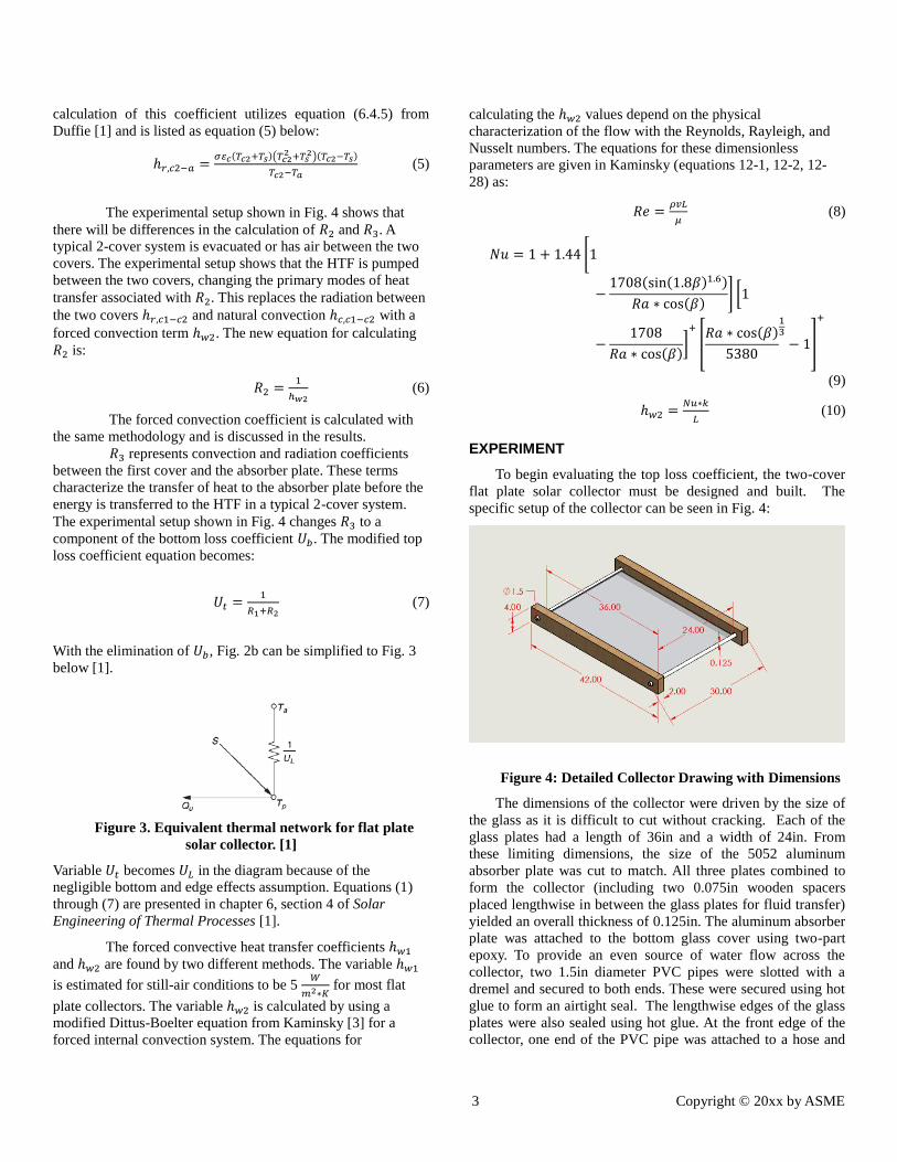
Figure 4: Detailed Collector Drawing with Dimensions

The dimensions of the collector were driven by the size of

the glass as it is difficult to cut without cracking. Each of the

glass plates had a length of 36in and a width of 24in. From

these limiting dimensions, the size of the 5052 aluminum

absorber plate was cut to match. All three plates combined to

form the collector (including two 0.075in wooden spacers

placed lengthwise in between the glass plates for fluid transfer)

yielded an overall thickness of 0.125in. The aluminum absorber

plate was attached to the bottom glass cover using two-part

epoxy. To provide an even source of water flow across the

collector, two 1.5in diameter PVC pipes were slotted with a

dremel and secured to both ends. These were secured using hot

glue to form an airtight seal. The lengthwise edges of the glass

plates were also sealed using hot glue. At the front edge of the

collector, one end of the PVC pipe was attached to a hose and

4 Copyright © 20xx by ASME

the other end was sealed with an end cap to ensure that the only

medium for water to flow was between the glass covers. The

slotted PVC pipe was also sealed to the collector on both ends

using hot glue. At the back edge of the solar collector, the PVC

pipe also had one end sealed with an end cap and the other end

open to provide a single outlet for the water flow. To create

structural support, two wooden 2”x4”’s of 42in length were

placed on the outer edges of the solar collector. Two holes in

each plank were drilled to allow the PVC pipe to fit through as

demonstrated in Fig. 4.

The mass flow rate through the collector was evaluated by

measuring the length of time required to fill an empty container

with water from the hose. The weight of the volume of water

within the container was then determined with a scale

calibrated to zero with the weight of the container. To minimize

error, three iterations were conducted and then averaged. Table

1 in the results section shows the data from that process.

To obtain the temperature reading required for calculating

the top loss coefficient, an accurate measurement system must

be used. This experiment utilized a block code with LabView

software in parallel with a National Instruments cDAQ-9171

with thermocouple capabilities [6].

A total of 5 k-type (chromel-alumel) thermocouples were

placed at the fluid inlet, fluid outlet, top of the glass cover,

bottom of the absorber plate, and the edge of the collector. The

sensitivity of this type of thermocouple is 41𝜇𝑉

℃, which

exceeded the accuracy required for the scope of this project [2].

For surface temperature measurements, the thermocouple ends

were attached with good contact using electrical tape. For the

inlet and outlet water temperatures, the thermocouples were

placed directly into the fluid streams. These locations can be

seen in Fig. 5:

Figure 5. Thermocouple Locations

A photo of the actual two-cover flat plate solar collector

assembly can be seen in Fig. 6:

Figure 6. Assembled Two-Cover Flat Plate Solar

Collector

The experiment was conducted on November 11, 2015

from 4:00 pm to 4:15 pm in Tempe, Arizona. The global

horizontal insolation value for this time is 269 W/m^2. Time

was cut short due to shadow effects. Ambient temperature (𝑇𝑎)

was recorded as 18.99℃. The mass flow rate (�̇�) of water

passing through the collector is the average taken from Table 1,

0.0288𝑘𝑔

𝑠. Once these values were determined, the solar

collector was placed horizontally (𝛽 = 0) in direct sunlight

with thermocouples attached. The hose was then attached to

the inlet and was allowed five minutes to reach steady state

before data was recorded.

RESULTS AND DISCUSSION

The data from the calculation of the mass flow rate is

presented below:

Table 1. Mass Flow Rate Measurements

Trial Mass of 𝑯𝟐𝑶 Time to Fill Mass Flow Rate

1 0.151 kg 5.30 s 0.0281 𝑘𝑔

𝑠

2 0.175 kg 5.95 s 0.0294 𝑘𝑔

𝑠

3 0.165 kg 5.68 s 0.0290 𝑘𝑔

𝑠

Average 0.0288 𝑘𝑔

𝑠

The data from the test setup was also collected and was

processed in MATLAB. Fig. 7 shows the inlet and outlet HTF

temperatures over time.

5 Copyright © 20xx by ASME

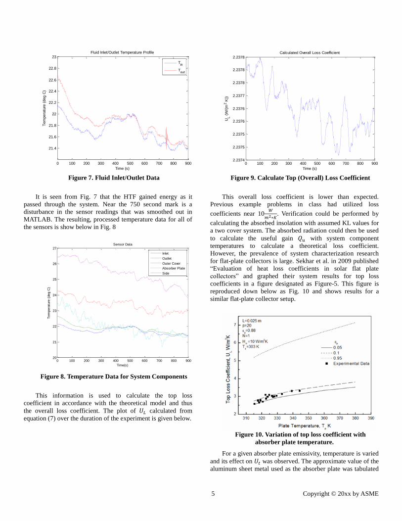
Figure 7. Fluid Inlet/Outlet Data

It is seen from Fig. 7 that the HTF gained energy as it

passed through the system. Near the 750 second mark is a

disturbance in the sensor readings that was smoothed out in

MATLAB. The resulting, processed temperature data for all of

the sensors is show below in Fig. 8

Figure 8. Temperature Data for System Components

This information is used to calculate the top loss

coefficient in accordance with the theoretical model and thus

the overall loss coefficient. The plot of 𝑈𝐿 calculated from

equation (7) over the duration of the experiment is given below.

Figure 9. Calculate Top (Overall) Loss Coefficient

This overall loss coefficient is lower than expected.

Previous example problems in class had utilized loss

coefficients near 10𝑊

𝑚2∗𝐾. Verification could be performed by

calculating the absorbed insolation with assumed KL values for

a two cover system. The absorbed radiation could then be used

to calculate the useful gain 𝑄𝑢 with system component

temperatures to calculate a theoretical loss coefficient.

However, the prevalence of system characterization research

for flat-plate collectors is large. Sekhar et al. in 2009 published

“Evaluation of heat loss coefficients in solar flat plate

collectors” and graphed their system results for top loss

coefficients in a figure designated as Figure-5. This figure is

reproduced down below as Fig. 10 and shows results for a

similar flat-plate collector setup.

Figure 10. Variation of top loss coefficient with

absorber plate temperature.

For a given absorber plate emissivity, temperature is varied

and its effect on 𝑈𝑡 was observed. The approximate value of the

aluminum sheet metal used as the absorber plate was tabulated

0 100 200 300 400 500 600 700 800 900

21.4

21.6

21.8

22

22.2

22.4

22.6

22.8

23

Time (s)

Tem

pera

ture

(deg C

)

Fluid Inlet/Outlet Temperature Profile

Tin

Tout

0 100 200 300 400 500 600 700 800 90020

21

22

23

24

25

26

27

Time(s)

Tem

pera

ture

(deg C

)

Sensor Data

Inlet

Outlet

Outer Cover

Absorber Plate

Side

0 100 200 300 400 500 600 700 800 9002.2374

2.2375

2.2375

2.2376

2.2376

2.2377

2.2378

2.2378

2.2378

Time (s)

UL (

W/(

m2 K

))

Calculated Overall Loss Coefficient

6 Copyright © 20xx by ASME

to be .09 [7]. The approximate temperature of the absorber plate

is 296K. Extrapolation of the data curves yields a 𝑈𝑡 value at

about 2.2, very near to the experimental results demonstrated in

Fig. 9. These results are consistent with each other, as well as

the low variation of the y-axis in Fig. 9.

It is important to note that edge and bottom losses do exist,

but their effects are not as prevalent as top losses. Utilizing

equation 6.4.11 from Duffie, an approximate edge loss

coefficient was calculated to be:

𝑈𝑒 =𝑘𝑎𝑖𝑟

𝑡𝑖𝑛𝑠∗ 𝑃 ∗

𝑡𝑐𝑜𝑙

𝐴𝑐= .1437

𝑊

𝑚2∗𝐾,

Where,

The difference in magnitude of the edge effects confirms

that they are negligible. This concept was reinforced by the fact

that the collector was built with only a 0.125in edge thickness,

and hot glue was used to seal the sides. Due to the fact that

0.125 inches is an extremely short side length, and only the

wooden 2x4’s used as framework for the collector served to

insulate the sides, the edge losses had the potential to be larger

but still were considerably smaller than the top losses. In

regards to bottom losses, only convection could be a viable

mode of heat loss, and even so it would pale in comparison to

convective losses at the top of the collector because of the test

setup’s proximity to the ground. The spacing of the absorber

plate from the ground results in an absence of conductive

mediums. This is because conductive heat transfer requires two

or more solids to be in contact [3]. The same assumption is

applicable to the top of the solar collector. Losses due to

radiation are also negligible at the bottom of the collector for a

few reasons. The net rate of heat transfer due to radiation is

given by equation (5), which demonstrates reliance on

temperature differences between the surface in question and the

surroundings [4]. The temperature difference between the

absorber plate and the surroundings was only a few degrees and

the structural components acted like a black box to contain all

the radiation. These conditions lead the radiative terms to be

very small.

CONCLUSIONS

The experimental results matched the results from other

flat-plate characterization research projects. The experimental

results also show the potential of solar thermal applications. A

simple two-cover flat-plate collector was able to be constructed

out of commonly available materials. Even with low sunlight

conditions in November, a marked increase in temperature was

able to be recorded. It was determined that losses through the

top of the collector dominated all other collector losses.

Neglecting edge and bottom losses means that calculation of

the overall collector loss coefficient can be performed readily,

which in turn allows for other useful information such as fluid

exit temperatures to be calculated easily. The experimental

results corresponding to 𝑈𝐿=2.2375 𝑊

𝑚2∗𝐾 illustrates the

reproducibility of this simple geometry.

Certain limitations impeded the ability to get higher

temperature differences and calculate other useful system

parameters. The experiment required significant planning and

budgeting by the three team members, who had limited

resources compared to other research groups. Those resources

could lead to greater accuracy and more distinct results with

access to more expensive materials. For example, commercially

built flat plate collectors typically maximize surface

absorptivity of absorber plates at 95%, while the surface

absorptivity of the aluminum absorber plate in this experiment

was 65% at best [7][8]. Increasing absorber plate absorptivity

without sacrificing low level emissivity requires special types

of glazing of which the researchers’ did not have access. Glass

cover transmittance could similarly have been optimized

through tempering, and usage of more specialized adhesives

could have further increased heat transfer efficiency within the

collector. Lastly, perhaps the most obvious experimental

improvement would be to test the collector in summer months

rather than winter to increase the levels of incident solar

irradiation. For future work, each of these limitations could be

addressed to benefit the experimental results from testing.

RECOMMENDATIONS

The test data shows an increasingly smaller temperature

difference around the time of 450 seconds. This is due to

shading from the sun’s movement. Any future tests would

require analysis of the testing stage to ensure proper operation

can continue for extended periods of time without moving the

experimental setup. It is recommended that additional research

be performed in order to characterize system parameters for

elaborate systems to better optimize new collector geometries,

such as “sea shell” geometry CPC’s.

REFERENCES

[1] J. A. Duffie and W. A. Beckman, “Flat-Plate Collectors,” in

Solar Engineering of Thermal Processes, 4th ed., Hoboken,

New Jersey: John Wiley and Sons, Inc, 2013, pp. 236–321.

[2] “Type K Thermocouple,” Thermometricscorp.com, 2014.

[Online]. Available at:

http://www.thermometricscorp.com/thertypk.html. [Accessed:

Dec-2015].

[3] D. Kaminski and M. K. Jensen, Introduction to Thermal and

Fluids Engineering. Hoboken, N.J.: Wiley, 2005.

[4] Y. A. Engel, Introduction to Thermodynamics and Heat

Transfer, International. New York: McGraw-Hill, 1997.

[5] “Emissivity Coefficients of Some Common Materials,”

2015. [Online]. Available at:

http://www.engineeringtoolbox.com/emissivity-coefficients-

d_447.html. [Accessed: Dec-2015].

7 Copyright © 20xx by ASME

[6]“NI cDAQ-9171 NI CompactDAQ 1-Slot USB Chassis.”

[Online]. Available

at: http://sine.ni.com/nips/cds/view/p/lang/en/nid/209817.

[Accessed: May-2015].

[6] “Flat Plate Collectors,” Power from the Sun, Jun-2013.

[Online]. Available at:

http://www.powerfromthesun.net/book/chapter06/chapter06.ht

ml. [Accessed: Dec-2015].

[7] “Emissivity Coefficients of some common Materials,”

Emissivity Coefficients of some common Materials. [Online].

Available at: http://www.engineeringtoolbox.com/emissivity-

coefficients-d_447.html. [Accessed: May-2015].

[8] “Surface Absorptivity,” Surface Absorptivity, 2015.

[Online]. Available at:

http://www.engineeringtoolbox.com/radiation-surface-

absorptivity-d_1805.html. [Accessed: Dec-2015].

Statistical Methods of Minimizing Risk for Small- Scale Wind Energy Investments

By Erik Misiak and Ian McLeod Professor Calhoun

Dec. 2nd, 2014

Executive Summary

The purpose of this project is to explore ways in which the typical individual could sample local data in order to better understand the available wind power in their region. The project is focused on using past data to extrapolate on potential returns in energy and money. This is intended as an alternative to expensive meteorological software. The project purpose is accomplished using statistical analyses in Matlab, such as discriminant analyses, multiple linear regressions, t-tests for comparison, and other methods of estimating probabilities. An estimation of potential power generation over a six-month period in Cold Bay, Alaska, is achieved. An explanation of the business impact of operating small-scale, residential turbines is also provided. It is recommended that the reader employ the methods in this paper toward implementing their own turbine, and thus contributing to the global shift toward renewable energy.

McLeod and Misiak 2

Introduction

A. Problem Statement In the modern energy market, alternative energies such as solar and wind

power are becoming more and more competitive against fossil fuels. However, reusable energy is not currently as reliable as fossil fuels for human needs. Of the many issues brought about, it can be difficult to select a site to farm wind because of inaccuracies in wind power estimation techniques. Advances in technology such as lidar equipment and meteorological software have significantly reduced the risk involved in commercial wind farm investments. However, these technologies are still so rare and expensive that the average citizen cannot afford them. This limits wind farming potential. The purpose of this project is to demonstrate how the average individual might take published data and employ statistical methods towards understanding the nature of wind speeds in their area. A theoretical utility for this knowledge could be setting up a personal wind farm on a residential property, or perhaps even designing a small-scale wind farm. The ability to use statistical estimation to predict areas that can produce the most energy is a vital resource for implementing personal wind turbines. Wind power is reliant on sustained wind speeds.

The business aspects pushing alternative energies can also be complex and multidimensional. State and federal agendas often conflict, and it appears that many people are uneducated about the energy resources they have available. It is the objective of this project to present the reader with simple energy policy knowledge in addition to statistical techniques regarding wind energy. Understanding these principles can empower the average citizen to defy the unpredictability in weather and feel comfortable operating their own turbine.

B. Background Information

As global dependency on coal continues to threaten the environment, alternative energy is on the rise. Many states have instituted a percentage quota of renewable energy to reach within the next few decades. Wind energy has become a leader in the pursuit of clean energy sources. New ideas are being explored every day in terms of capturing wind power, however a significant portion of the business aspect of energy relies on prediction. As any meteorologist can attest, it is very difficult to predict wind speeds since they are a byproduct of global changes in weather and chaotic variables. However, statistics can be employed in order to determine locations where there is a high probability of sustained wind speeds. To demonstrate this process, the selected location for this report was Cold Bay, Alaska since it is a relatively unexplored area in terms of wind energy. Cold Bay rigorously documents statistics in relation to wind energy in an online database as well. While sustained wind speeds may be lower in Alaska than in the contiguous United States, it is interesting to examine the possibility of lucrative power generation from a conditional probability standpoint. Such results can be a testament to the true versatility of wind energy.

McLeod and Misiak 3

C. Design Considerations

It is important to take caution when exploring statistics since false interpretations can proliferate. As the law of large numbers states, the larger the sample size the closer the statistics of the observations approach population parameters. In this project, yearly data consisting of hundreds of data points was examined. The data was taken from Alaska Energy Authority, which has an extensive inventory of statistics. As with any statistical method, error must be accounted for , and the student’s took caution not to extrapolate results beyond reasonable applications.

Procedure and Results

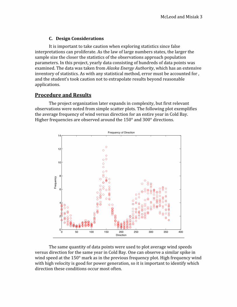
The project organization later expands in complexity, but first relevant observations were noted from simple scatter plots. The following plot exemplifies the average frequency of wind versus direction for an entire year in Cold Bay. Higher frequencies are observed around the 150° and 300° directions.

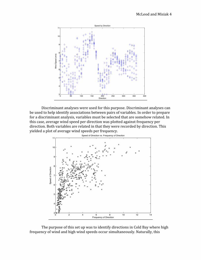
The same quantity of data points were used to plot average wind speeds versus direction for the same year in Cold Bay. One can observe a similar spike in wind speed at the 150° mark as in the previous frequency plot. High frequency wind with high velocity is good for power generation, so it is important to identify which direction these conditions occur most often.

McLeod and Misiak 4

Discriminant analyses were used for this purpose. Discriminant analyses can be used to help identify associations between pairs of variables. In order to prepare for a discriminant analysis, variables must be selected that are somehow related. In this case, average wind speed per direction was plotted against frequency per direction. Both variables are related in that they were recorded by direction. This yielded a plot of average wind speeds per frequency.

The purpose of this set up was to identify directions in Cold Bay where high frequency of wind and high wind speeds occur simultaneously. Naturally, this

McLeod and Misiak 5

combination is ideal for wind energy production. Normally, sustained wind speeds of 12 mph are typical constraints for wind farm investment. However, as observed in the previous plot, most wind speeds average below 9 mph in Cold Bay. Thus, it may not be economical to operate a wind turbine throughout the entire year. The goal of subsequent discriminant analyses is to identify directions and times of year where the probability of sustained wind speed occurring above 9 mph is high. This is similar to a conditional probability analysis. In other words, it is desirable to identify directions where the probability of wind speed occurring above 9 mph exists given also that a high frequency of wind exists in that direction. Quadratic discriminant classifiers were employed towards toward this end as well.

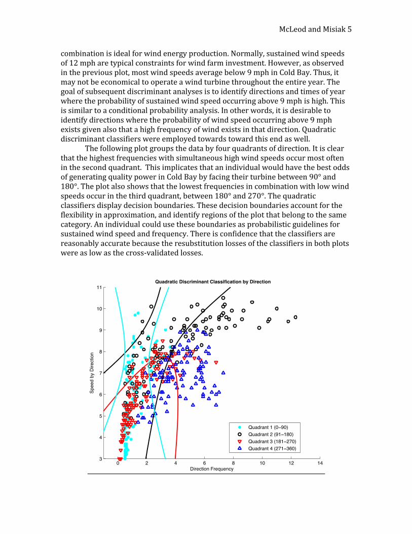
The following plot groups the data by four quadrants of direction. It is clear that the highest frequencies with simultaneous high wind speeds occur most often in the second quadrant. This implicates that an individual would have the best odds of generating quality power in Cold Bay by facing their turbine between 90° and 180°. The plot also shows that the lowest frequencies in combination with low wind speeds occur in the third quadrant, between 180° and 270°. The quadratic classifiers display decision boundaries. These decision boundaries account for the flexibility in approximation, and identify regions of the plot that belong to the same category. An individual could use these boundaries as probabilistic guidelines for sustained wind speed and frequency. There is confidence that the classifiers are reasonably accurate because the resubstitution losses of the classifiers in both plots were as low as the cross-validated losses.

McLeod and Misiak 6

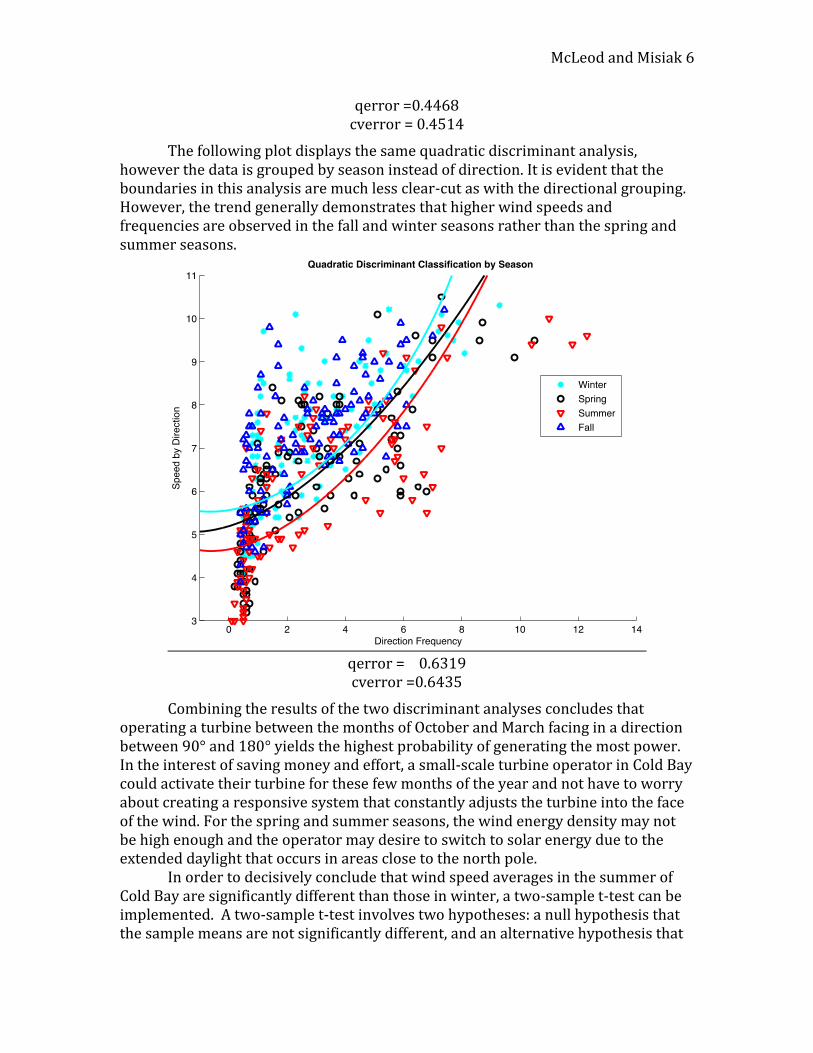
qerror =0.4468 cverror = 0.4514

The following plot displays the same quadratic discriminant analysis, however the data is grouped by season instead of direction. It is evident that the boundaries in this analysis are much less clear-cut as with the directional grouping. However, the trend generally demonstrates that higher wind speeds and frequencies are observed in the fall and winter seasons rather than the spring and summer seasons.

qerror = 0.6319 cverror =0.6435

Combining the results of the two discriminant analyses concludes that operating a turbine between the months of October and March facing in a direction between 90° and 180° yields the highest probability of generating the most power. In the interest of saving money and effort, a small-scale turbine operator in Cold Bay could activate their turbine for these few months of the year and not have to worry about creating a responsive system that constantly adjusts the turbine into the face of the wind. For the spring and summer seasons, the wind energy density may not be high enough and the operator may desire to switch to solar energy due to the extended daylight that occurs in areas close to the north pole.

In order to decisively conclude that wind speed averages in the summer of Cold Bay are significantly different than those in winter, a two-sample t-test can be implemented. A two-sample t-test involves two hypotheses: a null hypothesis that the sample means are not significantly different, and an alternative hypothesis that

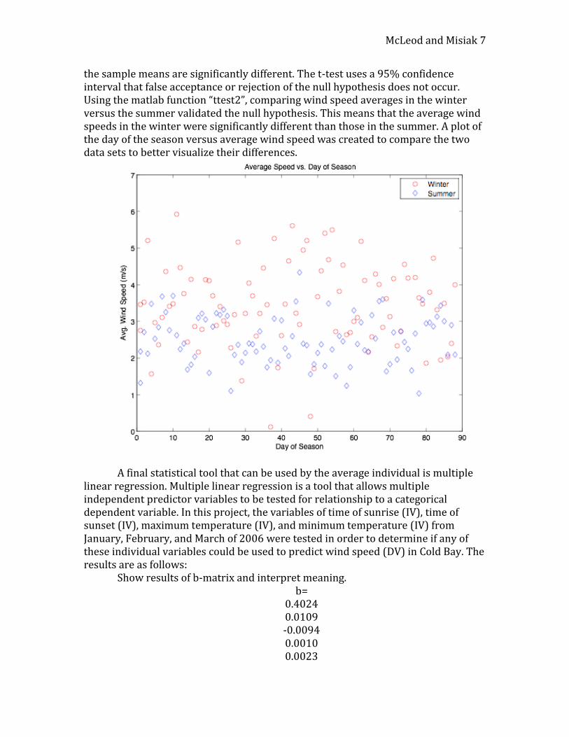
McLeod and Misiak 7

the sample means are significantly different. The t-test uses a 95% confidence interval that false acceptance or rejection of the null hypothesis does not occur. Using the matlab function “ttest2”, comparing wind speed averages in the winter versus the summer validated the null hypothesis. This means that the average wind speeds in the winter were significantly different than those in the summer. A plot of the day of the season versus average wind speed was created to compare the two data sets to better visualize their differences.

A final statistical tool that can be used by the average individual is multiple

linear regression. Multiple linear regression is a tool that allows multiple independent predictor variables to be tested for relationship to a categorical dependent variable. In this project, the variables of time of sunrise (IV), time of sunset (IV), maximum temperature (IV), and minimum temperature (IV) from January, February, and March of 2006 were tested in order to determine if any of these individual variables could be used to predict wind speed (DV) in Cold Bay. The results are as follows:

Show results of b-matrix and interpret meaning. b=

0.4024 0.0109 -0.0094 0.0010 0.0023

McLeod and Misiak 8

Show results of stats and interpret meaning. R^2 =[0.0062] Fstat =[0.1319] Prob =[0.9703] Variance =[1.443]

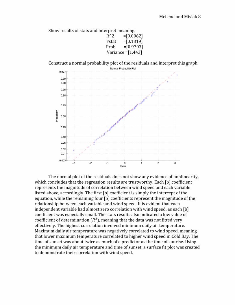
Construct a normal probability plot of the residuals and interpret this graph.

The normal plot of the residuals does not show any evidence of nonlinearity,

which concludes that the regression results are trustworthy. Each [b] coefficient represents the magnitude of correlation between wind speed and each variable listed above, accordingly. The first [b] coefficient is simply the intercept of the equation, while the remaining four [b] coefficients represent the magnitude of the relationship between each variable and wind speed. It is evident that each independent variable had almost zero correlation with wind speed, as each [b] coefficient was especially small. The stats results also indicated a low value of coefficient of determination (𝑅2), meaning that the data was not fitted very effectively. The highest correlation involved minimum daily air temperature. Maximum daily air temperature was negatively correlated to wind speed, meaning that lower maximum temperature correlated to higher wind speed in Cold Bay. The time of sunset was about twice as much of a predictor as the time of sunrise. Using the minimum daily air temperature and time of sunset, a surface fit plot was created to demonstrate their correlation with wind speed.

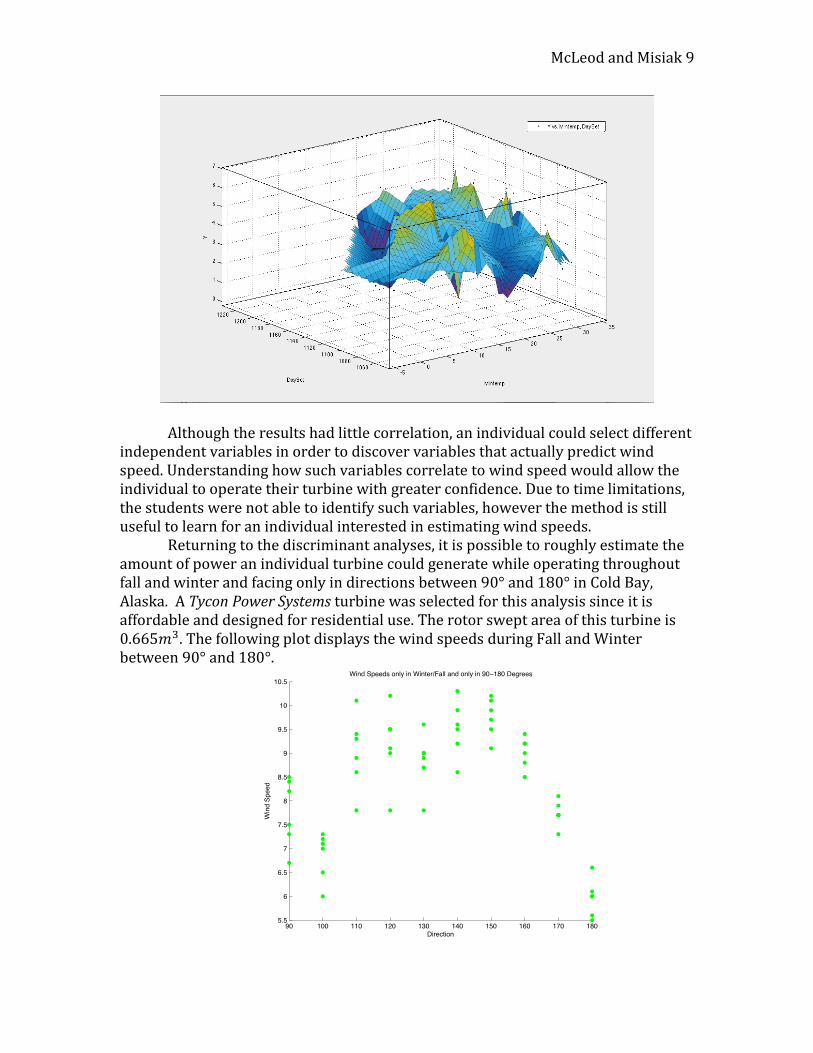
McLeod and Misiak 9

Although the results had little correlation, an individual could select different

independent variables in order to discover variables that actually predict wind speed. Understanding how such variables correlate to wind speed would allow the individual to operate their turbine with greater confidence. Due to time limitations, the students were not able to identify such variables, however the method is still useful to learn for an individual interested in estimating wind speeds.

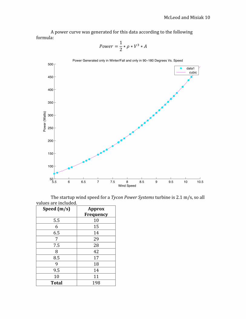
Returning to the discriminant analyses, it is possible to roughly estimate the amount of power an individual turbine could generate while operating throughout fall and winter and facing only in directions between 90° and 180° in Cold Bay, Alaska. A Tycon Power Systems turbine was selected for this analysis since it is affordable and designed for residential use. The rotor swept area of this turbine is 0.665𝑚3. The following plot displays the wind speeds during Fall and Winter between 90° and 180°.

McLeod and Misiak 10

A power curve was generated for this data according to the following formula:

𝑃𝑜𝑤𝑒𝑟 =1

2∗ 𝜌 ∗ 𝑉3 ∗ 𝐴

The startup wind speed for a Tycon Power Systems turbine is 2.1 m/s, so all values are included.

Speed (m/s) Approx Frequency

5.5 10

6 15

6.5 14

7 29

7.5 28

8 42

8.5 17

9 18

9.5 14

10 11

Total 198

McLeod and Misiak 11

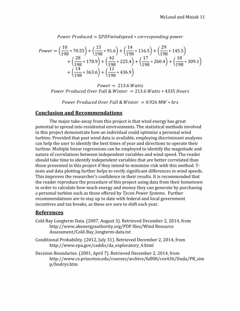
𝑃𝑜𝑤𝑒𝑟 𝑃𝑟𝑜𝑑𝑢𝑐𝑒𝑑 = Σ𝑃𝐷𝐹𝑤𝑖𝑛𝑑𝑠𝑝𝑒𝑒𝑑 ∗ 𝑐𝑜𝑟𝑟𝑒𝑠𝑝𝑜𝑛𝑑𝑖𝑛𝑔 𝑝𝑜𝑤𝑒𝑟

𝑃𝑜𝑤𝑒𝑟 = (10

198∗ 70.55) + (

15

198∗ 91.6) + (

14

198∗ 116.5) + (

29

198∗ 145.5)

+ (28

198∗ 178.9) + (

42

198∗ 225.4) + (

17

198∗ 260.4) + (

18

198∗ 309.1)

+ (14

198∗ 363.6) + (

11

198∗ 436.9)

𝑃𝑜𝑤𝑒𝑟 = 213.6 𝑊𝑎𝑡𝑡𝑠

𝑃𝑜𝑤𝑒𝑟 𝑃𝑟𝑜𝑑𝑢𝑐𝑒𝑑 𝑂𝑣𝑒𝑟 𝐹𝑎𝑙𝑙 & 𝑊𝑖𝑛𝑡𝑒𝑟 = 213.6 𝑊𝑎𝑡𝑡𝑠 ∗ 4335 𝐻𝑜𝑢𝑟𝑠

𝑃𝑜𝑤𝑒𝑟 𝑃𝑟𝑜𝑑𝑢𝑐𝑒𝑑 𝑂𝑣𝑒𝑟 𝐹𝑎𝑙𝑙 & 𝑊𝑖𝑛𝑡𝑒𝑟 = 0.926 𝑀𝑊 ∗ ℎ𝑟𝑠

Conclusion and Recommendations

The major take-away from this project is that wind energy has great potential to spread into residential environments. The statistical methods involved in this project demonstrate how an individual could optimize a personal wind turbine. Provided that past wind data is available, employing discriminant analyses can help the user to identify the best times of year and directions to operate their turbine. Multiple linear regressions can be employed to identify the magnitude and nature of correlations between independent variables and wind speed. The reader should take time to identify independent variables that are better correlated than those presented in this project if they intend to minimize risk with this method. T-tests and data plotting further helps to verify significant differences in wind speeds. This improves the researcher’s confidence in their results. It is recommended that the reader reproduce the procedure of this project using data from their hometown in order to calculate how much energy and money they can generate by purchasing a personal turbine such as those offered by Tycon Power Systems. Further recommendations are to stay up to date with federal and local government incentives and tax breaks, as these are sure to shift each year.

References

Cold Bay Longterm Data. (2007, August 3). Retrieved December 2, 2014, from http://www.akenergyauthority.org/PDF files/Wind Resource Assessment/Cold-Bay_longterm-data.txt

Conditional Probability. (2012, July 31). Retrieved December 2, 2014, from http://www.epa.gov/caddis/da_exploratory_4.html

Decision Boundaries. (2001, April 7). Retrieved December 2, 2014, from http://www.cs.princeton.edu/courses/archive/fall08/cos436/Duda/PR_simp/bndrys.htm

McLeod and Misiak 12

Discriminant Analysis. (n.d.). Retrieved December 2, 2014, from http://www.mathworks.com/help/stats/discriminant-analysis.html?refresh=true#brah8i2

Horizontal Wind Turbine. (2010, December 14). Retrieved December 2, 2014, from http://www.flyteccomputers.com/ext/Tycon Power/TPW-200-12.pdf

Joint, Marginal & Conditional Frequencies: Definitions, Differences & Examples. (n.d.). Retrieved December 2, 2014, from http://education-portal.com/academy/lesson/joint-marginal-conditional-frequencies-definitions-differences-examples.html#transcript

Multiple Regression. (2009, September 19). Retrieved December 2, 2014, from http://peoplelearn.homestead.com/MULTIVARIATE/Module11MultipRegress1.html

Wind Power: A Clean and Renewable Energy. (2014, June 17). Retrieved December 2, 2014, from http://www.renewableenergyst.org/wind.htm