i

TIME SERIES MODELING USING MARKOV AND ARIMA MODELS

MOHD KHAIRUL IDLAN BIN MUHAMMAD

A report submitted in partial fulfillment of the requirements for the award of the degree of

Master of Engineering (Civil – Hydraulic & Hydrology)

Faculty of Civil Engineering Universiti Teknologi Malaysia

JANUARY 2012

iii

DEDICATION

Special dedication to my beloved father and mother

Mr. Muhammad bin Ismail

and

Madam Siti Maznah binti Abdullah

and

My inspiration…

Jazakumullahu khairan for all love and inspiration

throughout the entire creation of this thesis.

iv

ACKNOWLEDGEMENT

Assalammualaikum w.b.t.

Alhamdulillah, all praise to Allah S.W.T for the gift of life and what I have achieved

today.

Appreciation goes to my family for their prayers, moral and financial support. May

Allay reward you abundantly.

My sincere and deepest gratitude goes to my supervisor, Dr. Sobri Harun for his

guidance, encouragement and support in completing this master project.

My gratitude to Dr. Muhammad Askari for his invaluable suggestions, guidance, and

encouragement.

Last but not least, to all my lecturers, classmates and friends, their help and supports are

really appreciated and will be remembers forever, InsyaALLAH. Thank you all

.

v

ABSTRACT

Streamflow forecasting plays important roles for flood mitigation and water

resources allocation and management. Inaccurate forecasting will cause losses to water

resources managers and users. The suitability of forecasting method depends on type and

number of available data. Thus, the objective of this study are to propose the streamflow

forecasting methods using Markov and ARIMA models and to inspect the accuracy of

Markov and ARIMA models in forecasting ability. Streamflow data of Sungai Bernam,

Selangor was used. Minitab and Microsoft Excel were used to model ARIMA and

Markov respectively. Criteria performance evaluation procedure that being used in this

study were Mean Absolute Percentage Error (MAPE), Root Mean Squared Error

(RMSE) and Chi-square test of Normality to inspect the forecasting accuracy of the

different models. The tentative model that best fits the criteria and meets the requirement

for ARIMA model is ARIMA (1,1,1)(0,1,1)12. From the criteria performance evaluation

procedure, ARIMA model has better performance of model for forecasting than Markov

model in this study. Therefore, ARIMA model has the ability to accurately predict the

future monthly streamflow for Sungai Bernam.

vi

ABSTRAK

Peramalan aliran sungai memainkan peranan yang penting untuk kawalan banjir

dan pengurusan air. Peramalan yang tidak tepat akan menyebabkan kerugian kepada

pihak pengurusan sumber air dan juga kepada pengguna. Kesesuaian kaedah peramalan

bergantung kepada jenis dan jumlah data yang tersedia. Maka, objektif kajian ini adalah

untuk mencadangkan kaedah peramalan aliran sungai dengan menggunakan model

Markov dan ARIMA dan untuk memeriksa ketepatan model Markov dan ARIMA dalam

membuat peramalan. Data aliran sungai Sungai Bernam telah digunakan. Minitab

digunakan untuk memodelkan model ARIMA dan Microsoft Excel digunakan untuk

memodelkan model Markov. Prosedur penilaian prestasi kriteria yang digunakan dalam

kajian ini ialah Mean Absolute Percentage Error (MAPE), Root Mean Squared error

(RMSE) dan ujian Chi-Squared untuk memeriksa ketepatan peramalan model-model

yang berlainan. Tentatif model yang terbaik sesuai dengan kriteria dan memenuhi

kehendak untuk model ARIMA ialah ARIMA (1,1,1)(0,1,1)12. Dari prosedur penilaian

prestasi kriteria, model ARIMA mempunyai prestasi yang lebih baik dalm membuat

ramalan berbanding dengan model Markov. Justeru, model ARIMA mempunyai

keupayaan untuk meramalkan dengan tepat aliran sungai di masa hadapan untuk Sungai

Bernam.

vii

TABLE OF CONTENTS

CHAPTER TITLE PAGE

DECLARATION ii DEDICATION iii ACKNOWLEDMENT iv ABSTRACT v ABSTRAK vi TABLE OF CONTENTS vii LIST OF TABLES x LIST OF FIGURES xi LIST OF APPENDICES xii LIST OF ABBREVIATIONS xiii

1 INTRODUCTION 1

1.1 Background of study 1

1.2 Problem Statement 4

1.3 Justification of the Study 4

1.4 Aim and Objectives 5

1.5 Scope of Study 5

2 LITERATURE REVIEW 6

2.1 Introduction 6

2.2 Time Series Model 7

2.3 Forecasting Time Series 8

2.4 Streamflow Forecasting Method 10

2.4.1 Markov Model 11

viii

2.4.2 ARIMA Theory 12

2.4.3 ARIMA Algorithms 13

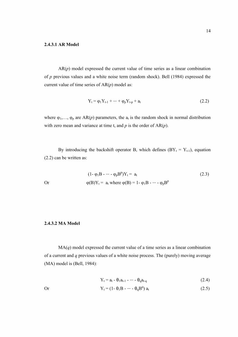
2.4.3.1 AR Model 14

2.4.3.2 MA Model 14

2.4.3.3 ARMA Model 15

2.4.3.4 ARIMA Model 16

2.5 Reviews on Markov Model 17

2.6 Review on ARIMA Model 18

2.7 Concluding Remarks 19

3 METHODOLOGY 20

3.1 Introduction 20

3.2 Markov Model 21

3.2.1 Statistical Parameters of Historical Data 21

3.2.2 Identification of Distribution 23

3.2.3 Generation of Random Numbers 24

3.2.4 Formulation of the Markov Model 24

3.3 ARIMA Model 25

3.3.1 Model Assumptions 26

3.3.1.1 Data Stationarity 26

3.3.1.2 Normal Distribution 27

3.3.1.3 Outlier 28

3.3.1.4 Missing Data 28

3.3.2 Model Procedure 29

3.3.2.1 Model Identification 29

3.3.2.2 Parameter Estimation 31

3.3.2.3 Diagnostic Checking 31

ix

3.3.3 Minitab Procedure 32

3.4 Model Comparison and Forecast Evaluation Measures 33

4 RESULTS AND DISCUSSION 35

4.1 Introduction 35

4.2 Estimation of Missing Data Values 36

4.3 Markov Model 38

4.3.1 Statistical Parameters of Historical Data 39

4.3.2 Identification of Distribution 40

4.3.3 Generation of Random Numbers 43

4.3.4 Streamflow Generation of Markov Model 45

4.3.5 Validation of Markov Model 46

4.4 ARIMA Model 48

4.4.1 Model Identification 49

4.4.2 Parameter Estimation 53

4.4.3 Diagnostic Checking 55

4.4.4 Streamflow Generation of ARIMA Model 58

4.4.5 Validation of ARIMA Model 59

3.4 Model Comparison and Forecast Evaluation Measures 60

5 CONCLUSION AND RECOMMENDATIONS 65

5.1 Conclusion 65

5.2 Recommendations 66

REFERENCES 68

APPENDICES A-G 72 - 81

x

LIST OF TABLES

TABLE NO. TITLE PAGE

4.1 Parameters of Monthly Historaical Data 40

4.2 Logarithmic Values of Observed Streamflow Data

for 1960-1970 42

4.3 Generation of Random Number for Year 2006 45

4.4 Model Streamflow for Year 2006 46

4.5 Accuracy of the Markov Model 47

4.6 General Theoretical ACF and PACF of ARIMA

models

51

4.7 Final Estimates of Parameter for ARIMA (1,1,1)

(1,1,1)12

54

4.8 Final Estimates of Parameter for ARIMA (1,1,1)

(0,1,1)12

54

4.9 Modified Box-Pierce (Ljung Box) Chi-Square

statistic for ARIMA (1,1,1)(1,1,1)12

55

4.10 Modified Box-Pierce (Ljung Box) Chi-Square

statistic for ARIMA (1,1,1)(0,1,1)12

56

4.11 LSE and RMSE Test for ARIMA Tentative Model 56

4.12 Model Streamflow for Year 2006-2007 58

4.13 Accuracy of the ARIMA Model 60

4.14 Accuracy of the model 62

xi

LIST OF FIGURES

FIGURE NO. TITLE PAGE

2.1 Value of time series with forecast function at 50%

probability limits 9

3.1 Flowchart of ARIMA modeling 29

4.1 Linear Regression of Two Streamflow for 1962 36

4.2 Linear Regression of Rainfall and Streamflow 37

4.3 Linear Regression of Two Streamflow for 1993 38

4.4 Descriptive Statistics of Sungai Bernam Data 39

4.5 Probability Density Function 41

4.6 Cumulative Distribution Function 42

4.7 Cumulative Distribution Function of the Log-normal

Distribution

43

4.8 Comparison of Observed and Markov Flow 47

4.9 Flow Diagram of Box-Jenkins Methodology 48

4.10 Non stationary data of Sg. Bernam streamflow 50

4.11 Stationary data of Sg. Bernam streamflow 50

4.12 ACF after non-seasonal difference 51

4.13 PACF after non-seasonal difference 52

4.14 ACF after seasonal difference 52

4.15 PACF after seasonal difference 53

4.16 Comparison of Observed and ARIMA Model Flow 59

4.17 Model Comparison 61

4.18 Streamflow for actual and model 63

xii

LIST OF APPENDICES

APPENDIX TITLE PAGE

A Streamflow Data of Sungai Bernam 1960-2010 72

B Logarithmic of Observed Streamflow Data for 1960-2005 73

C Generation of Random Number for Year 2006-2010 74

D Markov Model Streamflow 75

E Performance Evaluation Procedure of Markov Model 76

F ARIMA Model Streamflow 78

G Performance Evaluation Procedure of ARIMA model 80

xiii

LIST OF ABBREVIATIONS

ACF - Autocorrelation Function

AD - Anderson Darling

AR - Autoregressive

ARIMA - Autoregressive Integrated Moving Average

DF - Degree of Freedom

K-S - Kolmogorov-Smirnov

LSE - Least Squared Error

MA - Moving Average

MAPE - Mean Absolute Percentage Error

PACF - Partial Autocorrelation Function

RMSE - Root Mean Square Error

R2 - Coefficient of Determination

S - Standard Deviation

SE - Standard Error

Sg. - Sungai

Χ2 - Chi-square

CHAPTER 1

INTRODUCTION

1.1 Background of Study

According to Bowerman and O’Connell (1993), predictions of future events and

conditions are called forecasts, and the act of making such predictions is called

forecasting. In many types of organizations, forecasting is very important as predictions

of future events must be incorporated into the decision-making process. In forecasting

events that will occur in the future, information concerning events that have occurred in

the past must be relied.

In order to prepare forecasts, past data need to be analyzed to identify a pattern

that can be used to describe it. Then, this pattern is extrapolated or extended into the

future. This forecasting technique rests on the assumption that the pattern that has been

identified will continue in the future to give good predictions. If the data pattern that has

been identified does not persist in the future, this indicates that the forecasting technique

used is likely to produce inaccurate predictions (Bowerman and O’Connell, 1993).

2

Most forecasting problems involve the use of time series data. In this study, time

series is used to prepare forecasts. Time series is formed from measurements of a

variable taken at regular intervals over time. It is a stochastic process which amounts to

a sequence of random variables. The hydrologic data of streamflows fall under the

category of time series (Gupta, 1989). Time series can be used in application of

forecasting of future values of a time series from current and past values, and can be

used to forecast streamflow (Box and Jenkins, 1976). Time series plots can reveal

patterns such as random, trends, level shifts, periods or cycles, unusual observations, or

a combination of patterns.

Streamflow forecasting plays important roles for flood mitigation and water

resources allocation and management. In water management, the high quality

streamflow forecast and efficient use of this forecast can give considerable economic

and social benefits. Short-term forecasting like hourly and daily forecasting is crucial for

flood warning and defense while long-term forecasting which is based on monthly,

seasonal or annual time series is very useful for reservoir operation, irrigation

management decision, drought mitigation and managing river treaties (Shalamu, 2009).

Recently, due to the increase in data availability from metering stations, real time

data retrieval and increasing computational capability with the development of more

robust methods and computer techniques, time series models have become quite popular

in streamflow forecasting (Wang, 2006). A considerable number of forecasting models

and methodologies have been developed and applied in streamflow forecasting due to

importance of hydrologic forecasting. In this study, Markov and ARIMA model have

been used in the modeling of monthly streamflow processes.

3

The Markov process considers that the value of streamflow at one time is

correlated with the value of the streamflow at an earlier period (i.e. a serial or

autocorrelation exists in the time series). In a first-order Markov process, this correlation

exists in two successive values of the events (Gupta, 1989).

The first order Markov model states that the value of a variable x in one time

period is dependent on the value of x in the preceding time period plus a random

component. Thus, the synthetic streamflow represent a sequence of numbers, each of

which consists of two parts, which are deterministic and random parts (Gupta, 1989).

Autoregressive Integrated Moving Average (ARIMA) which is often called

method of Box-Jenkins time series has good accuracy for short-term forecasting, but less

good accuracy for long-term forecasting. Usually, it will tend to become flat for a

sufficiently long period. ARIMA model ignores the independent variable completely,

and uses past and present values of dependent variable to produce accurate short-term

forecasting (Hendranata, 2003).

ARIMA is suitable when the observation of time series is statistically related to

the dependent. The purpose of this model is to determine good statistical relationships

between the variables that being predicted and the historical value of these variables, so

that forecasting can be performed with the model (Hendranata, 2003).

4

1.2 Problem Statement

There are many time series forecasting methods can be used to predict the

streamflow. However, not all of these methods can produce accurate forecasts.

Inaccurate forecasting will cause losses to water resources managers and users. The

suitability of forecasting method depends on type and number of available data. ARIMA

and Markov models must be inspected to determine the ability of this method to provide

accurate and reasonable monthly streamflow forecasting. Through statistical methods,

the accuracy of both models for forecasting monthly streamflow will be tested and

evaluated. ARIMA modeling approach and Markov model was employed to the data set

to further investigate the behavioral change in the streamflow. The result of the study

can be used as a reference guideline to the flood control as Markov and ARIMA models

best suited for short-term forecasting.

1.3 Justification of the Study

Monthly streamflow forecasting is an integral part of drought, irrigation and

reservoir operation management. Stochastic data generation aims to provide alternative

hydrologic data sequences that are likely to occur in future to assess the reliability of

alternative systems designs and policies, and to understand the variability in future

system performances. It is also very important to develop a stochastic hydrologic model

to generate the monthly streamflows and thus to estimate the future streamflows.

Through this model, it is wish that the problem on water shortage can be reduced.

Forecasting also can be used to give warning of extreme events like drought (Joomizan,

2010).

5

1.4 Aim and Objectives

The aim of this paper is to forecast streamflow by using appropriate time series

modeling approach. To achieve this aim, the following objectives have been identified:

1. To propose the streamflow forecasting methods using Markov and ARIMA

models.

2. To inspect the accuracy of Markov and ARIMA models in forecasting ability.

1.5 Scope of Study

In this study, two models of time series are used which are Markov model and

ARIMA model to predict the behavior of streamflow. Streamflow data of Sungai

Bernam, Selangor for the period of 1960 to 2010 were used for the application of the

model. The study area that located in southeast Perak and northeast Selangor is semi

developed area and the size is 186km2.

Streamflow data were obtained from station Sg. Bernam at Tanjung Malim

(Station No. 3615412). The data which is monthly streamflow were collected from the

Department of Irrigation and Drainage, Kuala Lumpur. Computer program that being

used for ARIMA model is Minitab 15 and Microsoft Excel is used for Markov model.

CHAPTER 2

LITERATURE REVIEW

2.1 Introduction

Generally, surface water hydrology is the basis to engineering design and sources

of water. High streamflow may cause disaster like flood and erosion. Short-term

forecasting is needed to control this. Meanwhile, low streamflow can disrupt water

supply to domestic user, industrial, generation of hydroelectric power and irrigation.

Here, long-term forecasting is useful to prevent this problem. Therefore, ability to

generate streamflow forecasting accurately can be used in water flow management and

flood control.

Modeling and forecasting time series has long been practiced by using different

statistical methods. Forecasting models of time series that are commonly used are

ARIMA, moving average, exponential smoothing, regression analysis, and Fourier series

analysis. In this study, Markov and ARIMA model are used to predict monthly

streamflow.

7

2.2 Time Series Model

A time series is a time-oriented or chronological sequence of observations on a

variable of interest (Montgomery et al., 2008). Time series models have become popular

in recent years since the publication of the book by Box and Jenkins (1970), and the

subsequent development of computer software for applying these models (Bell, 1984).

The time can be a discrete value, a time interval or a continuous function. The

hydrologic data of streamflows, precipitation, groundwater or lake levels, water

temperatures, or oxygen concentration fall under the category of time series. These data

can be deterministic, random, or a combination of the two (Gupta, 1989).

Many conventional statistical methods traditionally deals with models in which

the observations are assumed to be independent. However, a great deal of data in

business, economics, engineering and natural sciences occur in the form of time series

where observations are dependent. The systematic approach available for answering the

mathematical and statistical questions posed by these series of dependent observations is

called time series analysis. The objective of time series analysis is generally to

understand and identify the stochastic process that produced the observed series and then

to forecast future values of a series from past values alone (Akgun, 2003).

The analysis of a time series, in the time domain, is performed by a parameter

known as the serial correlation coefficient or the autocorrelation coefficient. This

parameter indicates the dependence in successive values of a time series. This

coefficient is determined for successive values (elements) and also for elements that are

various time intervals apart which known as lag period. A graph of the autocorrelation

coefficient against the lag period is known as the correlogram. If a correlogram shows

zero or nearly zero values for all lag periods, the process is purely random. A value close

to 1 will suggest a dominating deterministic process (Gupta, 1989).

8

The analysis of a time series in the frequency domain is done by the spectral

density that identifies the cyclic nature or periodicity in the series. The density indicates

the cycle in the deterministic data. In a purely random process it oscillates randomly.

The purpose of streamflow synthesis, however is not to analyze a time series but to

generate the data based on the series. This does not require the decomposition of the

time series by the analysis above but an understanding of its statistical properties to

reproduce series of similar statistical characteristics (Gupta, 1989).

2.3 Forecasting Time Series

Most forecasting problems involve the use of time series data. Montgomery et al.

(2008) stated that forecasting problems are often classified as short-term, medium term,

and long-term. Short-term forecasting problems involve predicting events only a few

time periods (days, weeks, months) into the future. Medium-term forecasts extend from

one to two years into the future, and long-term forecasting problems can extend beyond

that by many years. Short-term and medium-term forecasts are used for operations

management and development of projects while long-term forecasts can be used for

strategic planning.

In this study, we try to use Markov and ARIMA for long-term forecasting. As we

know, Markov and ARIMA models are best for short-term forecasting. Normally, short-

term and medium-term forecasts are based on identifying, modeling, and extrapolating

the patterns found in historical data. These historical data usually exhibit inertia and do

not change very drastically. Therefore, statistical methods are very useful for short-term

and medium-term forecasting (Montgomery et al., 2008).

9

The use at time t of available observations from a time series to forecasts its

value at some future time can provide a basis for (1) economic and business planning,

(2) production planning, (3) inventory and production control, and (4) control and

optimization of industrial processes (Box et al., 1994). As originally described by Brown

(1962), forecasts are usually needed over a period known as the lead time, which varies

with each problem. Usually, forecasts are made at time t by taking the current month Yt

and previous months Y1, Y2,…,Yt-1, to forecast at some future time Ft+1, Ft+2,…, Ft+m from

Y value forward.

In order to calculate best forecasts, it is necessary to specify their accuracy. The

accuracy of the forecasts may be expressed by calculating convenient set of probability

limits on either side of each forecast, such as 50% and 95%. It means that the realized

value of time series will be included within these limits with the stated probability when

it eventually happens. To illustrate, Figure 2.1 shows value of time series with forecast

made from origin t for lead time l together at 50% probability limits.

Figure 2.1: Value of time series with forecast function at 50% probability limits

(Source: Box et al., 1994)

10

2.4 Streamflow Forecasting Method

Being a natural phenomenon, streamflow has a random component. But, it is not

fully random because it has been observed that a low flow tends to follow low flow and

a high flow tends to follow high flow. The word “stochastic” is used to denote the

randomness in statistics but in hydrology it refers to a partial random sequence as well.

Therefore, the streamflow data that represent time series is actually involving a

stochastic process. Various stochastic processes are used for generating the hydrologic

data (Gupta, 1989).

Stochastic modeling of hydrologic time series has been widely used for planning

and management of water resources systems such as for reservoir sizing and forecasting

the occurrence of future hydrologic events. For example, stochastic models are used to

generate synthetic series of water supply that may occur in the future which are then

utilized for estimating the probability distribution of key decision parameters such as

reservoir storage size. Furthermore, stochastic models can be used for forecasting water

supplies and water demands in days, weeks, months and years in advance (Fortin et al.,

2004).

The previous rainfall and streamflow records can be utilized as model inputs for

forecasting the next time step ahead of the streamflow (Mohd Shafiek et al., 2005). This

study employs the previous streamflow records to forecast the streamflow discharge of

the following month.

There are some stochastic models that can be utilized for synthetic generation

and forecasting of hydrological process. Hydrologic processes such as monthly

streamflow may be well represented by stationary linear models such as Markov process

11

or autoregressive (AR) and autoregressive integrated moving average (ARIMA) models.

These models are usually capable of preserving the historical annual statistics, such as

the mean, variance, skewness and covariance (Fortin et al., 2004). In this study, Markov

and ARIMA models are used to predict future monthly streamflow.

2.4.1 Markov Model

The Markov process considers that the value of an event (i.e. streamflow) at one

time is correlated with the value of the event at an earlier period (i.e. a serial or

autocorrelation exists in the time series). In a first-order Markov process, this correlation

exists in two successive values of the events. The first order Markov model, which

constitutes the classic approach in synthetic hydrology, states that the value of a variable

x in one time period is dependent on the value of x in the preceding time period plus a

random component. Thus the synthetic flow for a stream represent a sequence of

numbers, each of which consists of two parts:

(2.1)

where is flow at ith time (ith number of a time series); di(t) is deterministic part at ith

time; and ei is random part at ith time. The values of ei are tied up with the historical data

by ensuring that they belong to the same frequency distribution and posses similar

statistical properties (mean, deviation, skewness) as the historical series (Gupta, 1989).

The various forms and combinations of deterministic and random component are

recognized as different models. Single season (annual) flow model of lag 1 is the

12

simplest model which assumes that the magnitude of the current flow is significantly

correlated with the previous flow value only. In the other hand, multiple-season models

divide the yearly flow into seasons or months (Gupta, 1989).

First order Markov Model has been successfully applied to many problems.

Examples include modeling sequential data using Markov chains, and solving control

problems posed in the Markov decision processes (MDP) framework. If the Markov

model’s parameters are estimated from data, the standard maximum likelihood estimates

consider the first order (single step) transitions only. But for many problems, the first

order conditional independence assumptions are not satisfied as a result of the higher

order transition probabilities can be poorly approximated by the learned model

(Joomizan, 2010).

The assumption of first order Markovian processes for representing the inflow

process of a reservoir has generally been considered in the literature as adequate for

most purposes. The development of models incorporating other approaches result in

extremely complex transition probability matrices (Wurbs, 2005).

2.4.2 ARIMA Theory

ARIMA is an abbreviation of AutoRegressive Integrated Moving Average

introduced by Box and Jenkins (Box et.al., 1994). As such, some authors refer to this

modeling approach as a Box and Jenkins model. Box-Jenkins model is stationary time

series model. Time series that generated from zero-mean, finite variance, and

13

uncorrelated variable is called a ‘white noise’ series which many useful models can be

constructed from it.

The ARIMA modeling is essentially an exploratory data-oriented approach that

has the flexibility of fitting an appropriate model which is adapted from the structure of

the data itself. The stochastic nature of the time series can be approximately modeled

with the aid of autocorrelation function and partial autocorrelation function; from which

information such as trend, random variables, periodic components, cyclic patterns and

serial correlation can be discovered. As a result, forecasts of the future values of the

series, with some degree of accuracy can be readily obtained (Ho and Xie, 1998).

Although ARIMA modeling is sophisticated in theory, but with the advent of

computer technology today, the iterative model building process and hence accurate

forecast can be aided and made simpler by the ease of many user-friendly statistical

software packages such as SAS, Statgraphics, Statistica and Minitab. An iterative three-

stage process, i.e. through model identification, parameter estimation and diagnostic

check is required to determine the adequacy of the proposed model (Ho and Xie, 1998).

2.4.3 ARIMA Algorithms

ARIMA contains three components, namely autoregressive (AR), Integrated (I)

and moving average (MA) parts. The AR part described the relationship between present

and past observations. The MA part represents the autocorrelation structure of error. The

I part represents the differencing level of the series to eliminate non-stationary

(Hasmida, 2009). It is usually denoted by (p,d,q)(P,D,Q) where p denotes order of auto-

regressive component, d denotes order of differencing, q denotes order of moving

average and (P,D,Q) denotes corresponding seasonal component.

14

2.4.3.1 AR Model

AR(p) model expressed the current value of time series as a linear combination

of p previous values and a white noise term (random shock). Bell (1984) expressed the

current value of time series of AR(p) model as:

Yt = φ1Yt-1 + ··· + φpYt-p + at (2.2)

where φ1,…, φp are AR(p) parameters, the at is the random shock in normal distribution

with zero mean and variance at time t, and p is the order of AR(p).

By introducing the backshift operator B, which defines (BYt = Yt-1), equation

(2.2) can be written as:

(1- φ1B - ··· - φpBp)Yt = at (2.3)

Or φ(B)Yt = at where φ(B) = 1- φ1B - ··· - φpBp

2.4.3.2 MA Model

MA(q) model expressed the current value of a time series as a linear combination

of a current and q previous values of a white noise process. The (purely) moving average

(MA) model is (Bell, 1984):

Yt = at - θ1at-1 - ··· - θqat-q (2.4)

Or Yt = (1- θ1B - ··· - θqBq) at (2.5)

15

Or Yt = θ(B) at.

where q is the order of MA(q), and θ coefficients are MA(q) model parameters.

2.4.3.3 ARMA Model

To increase flexibility when fitting actual time series, both autoregressive and

moving average operators are combined to give the ARMA (p,q) model (Bell, 1984):

Yt = φ1Yt-1 + ··· + φpYt-p + at - θ1at-1 - ··· - θqat-q (2.6)

which we write as:

(1- φ1B - ··· - φpBp)Yt = (1- θ1B - ··· - θqBq) at (2.7)

Or φ(B)Yt = θ(B) at.

The mixed type of series which are explained both by its own lagged values and

by lagged noise terms is called Autoregressive Moving-Average models of order (p,q).

This systematic class of stationary time series models carries great importance and

usefulness especially in real-life situations. If the process is stationary, a suitable ARMA

model can be used to represent the data. If it is nonstationary, differencing is applied to

make the model become stationary and this leads to ARIMA model (Akgun, 2003).

16

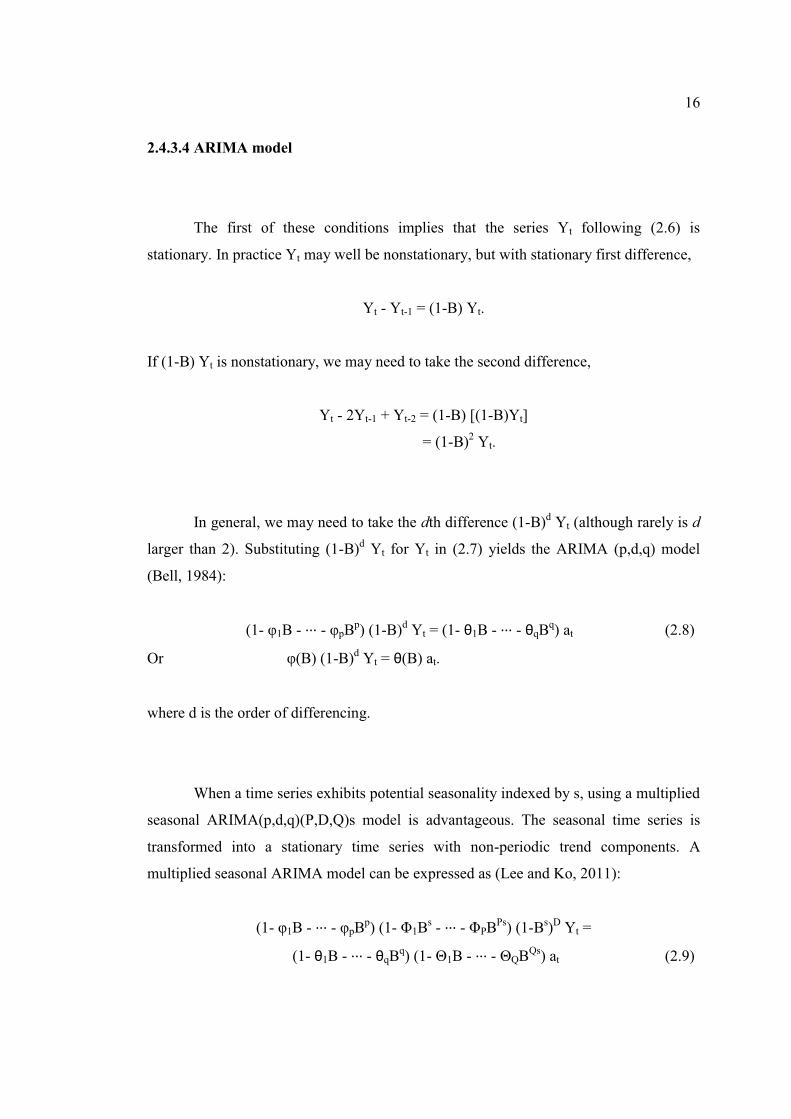
2.4.3.4 ARIMA model

The first of these conditions implies that the series Yt following (2.6) is

stationary. In practice Yt may well be nonstationary, but with stationary first difference,

Yt - Yt-1 = (1-B) Yt.

If (1-B) Yt is nonstationary, we may need to take the second difference,

Yt - 2Yt-1 + Yt-2 = (1-B) [(1-B)Yt]

= (1-B)2 Yt.

In general, we may need to take the dth difference (1-B)d Yt (although rarely is d

larger than 2). Substituting (1-B)d Yt for Yt in (2.7) yields the ARIMA (p,d,q) model

(Bell, 1984):

(1- φ1B - ··· - φpBp) (1-B)d Yt = (1- θ1B - ··· - θqBq) at (2.8)

Or φ(B) (1-B)d Yt = θ(B) at.

where d is the order of differencing.

When a time series exhibits potential seasonality indexed by s, using a multiplied

seasonal ARIMA(p,d,q)(P,D,Q)s model is advantageous. The seasonal time series is

transformed into a stationary time series with non-periodic trend components. A

multiplied seasonal ARIMA model can be expressed as (Lee and Ko, 2011):

(1- φ1B - ··· - φpBp) (1- Φ1Bs - ··· - ΦPBPs) (1-Bs)D Yt =

(1- θ1B - ··· - θqBq) (1- Θ1B - ··· - ΘQBQs) at (2.9)

17

Or φ(B)Φ(Bs) (1-Bs)D Yt = θ(B)Θ(Bs)at.

where D is the order of seasonal differencing, Φ(Bs) and Θ(Bs) are the seasonal AR(p)

and MA(q) operators respectively, which are defined as:

Φ(Bs) = 1- Φ1Bs - ··· - ΦPBPs

Θ(Bs) = 1- Θ1B - ··· - ΘQBQs

where Φ1,…, Φp are the seasonal AR(p) parameters and Θ1,…, Θp are the seasonal

MA(q) parameters.

To illustrate forecasting with ARIMA models, we shall use (2.9) written as:

Yt+l = Φ1Yn+l-1 + ··· + Φp+dYn+l-p-d + an+l - θ1an+l-1 - ··· - θqan+l-q (2.10)

for t = n + l. We shall assume we want to forecast Yn+l for l = 1, 2, … using data Yn, Yn-

1, …. For simplicity, we are assuming for now that the data set is long enough so that we

may effectively assume it extends into the infinite past.

2.5 Reviews on Markov Model

Naadimuthu and Lee (1982) proposed first order or lag one serially correlated

inflow. This means that the inflow of each month is dependent only on the inflow of the

previous month, forming a Markov chain. Markov chain method is stochastic method

that can be used to produce new time series of discharge of inflows based on available

time series of data (Adib and Majd, 2009).

18

According to Heiko (2000), Markov chains are stochastic processes that can be

parameterized by empirically estimating transition probabilities between discrete states

in the observed systems. The Markov chain of the first order is one for which each next

state depends only on immediately preceding one. Markov chains of second or higher

order are the processes in which the next state depends on two or more preceding ones.

Dalphin (1987) developed a lag-1 month-to-month Markov streamflow model in

which families of three-parameter Weibull distributions describe monthly streamflow

probabilistically, conditioned on streamflow in the preceding month.

2.6 Reviews on ARIMA Model

Tang et al. (1991) stated that ARIMA model is only good for short term

forecasting since it builds its forecast on previous observations. ARIMA model needs

long memory series, which are more inputs to provide more accurate forecasts. For long

memory series, more training patterns results in more accurate forecasts. This Box-

Jenkins model does not work well or does not work at all for short input series.

Ho and Xie (1998) proved that ARIMA model is a viable alternative that give

satisfactory results for repairable system reliability forecasting. Ayob and Amat (2004)

used ARIMA to represent water use behavior at Universiti Teknologi Malaysia. ARIMA

modeling method also can be applied to analyses the water quality and rainfall-runoff

data for Johor River recorded for a long period (Hasmida, 2009).

19

Maia et al. (2008) demonstrated that ARIMA exhibited a satisfactory

performance in forecasting interval series with either a linear or non-linear behavior and

are useful forecasting alternative to interval-valued time series. However, the hybrid

model using ARIMA and artificial neural network had better average performance.

A multiplicative seasonal autoregressive integrated moving average is applied to

the monthly streamflow forecasting of the Zayandehrud River in western Isfahan

province, Iran (Modarres, 2007). Nazuha (2010) used ARIMA to analyze monthly

Malaysia crude oil production. Besides that, Yurekli et al. (2004) used ARIMA to

simulate monthly maximum data of Cekerek Stream.

2.7 Concluding Remarks

Various techniques can be utilized for synthetic generation and forecasting of

hydrological process. Stochastic models can provide alternative hydrologic data

sequences that are likely to occur in the future to access the reliability of alternative

systems designs and policies, and to understand the variability in future system

performance.

Streamflow forecasting is an integral part of land management and water

resources management. Hydrologic processes such as monthly streamflow may be well

represented by stationary linear models such as Markov process or autoregressive (AR)

and autoregressive integrated moving average (ARIMA) models.

CHAPTER 3

METHODOLOGY

3.1 Introduction

Various stochastic processes are used for generating the hydrologic data of

streamflow. The models either developed or used in order to carry out this study are of

different types in terms of their purposes, capabilities, interfaces, inputs, and outputs.

These mainly include water balance model, reservoir simulation, and stochastic models.

The brief descriptions of the model development and considerations associated

with each of the models are presented in the following sections. The computation work

used the available historical data taken from Department of Irrigation and Drainage. The

relevant data is used in deriving the forecasting models. Markov and ARIMA modeling

methods have been proposed for streamflow forecasting of Sungai Bernam. The method

to determine the accuracy of these models in forecasting ability also will be discussed.

21

3.2 Markov Model

Gupta (1989) stated that the general Markov procedure of data synthesis comprises:

1. Determination of statistical parameters from the analysis of the historical

record

2. Identifying the frequency distribution of the historical data

3. Generating random numbers of the same distribution and statistical

characteristics

4. Constituting the deterministic part considering the persistence (influence

of previous flows) and combining with the random part.

3.2.1 Statistical Parameters of Historical Data

Four parameters that are important in a synthetic study are mean flow, standard

deviation, coefficient of skewness and correlation coefficient. The sample mean flow is

(Gupta, 1989):

(3.1)

Where,

mean observed (historical) flow

total numbers (values) of flow

ith number of observed flow

22

The sample estimate of the variance or standard deviation, S, which is a measure

of the variability of the data is given by (Gupta, 1989):

(3.2)

The sample of coefficient of skewness, g, which is a measure of the lack of symmetry, is

given by (Gupta, 1989):

(3.3)

The serial correlation coefficient is a measure of the extent to which a flow at

any time is affected by the flow at another time. The K-lag coefficient, in which the

effect extends by K time units is given by (Gupta, 1989):

(3.4)

The one-lag serial coefficient, in which the current flow is affected only by the

previous flow can be obtained by substituting K = 1. The additional lags should be

included as long as they produce a model that explains more about the pattern of flows

than one with fewer lag does (Fiering and Jackson, 1971).

23

3.2.2 Identification of Distribution

Generally, the distributions used in streamflow generation are normal, log-

normal and gamma families. The bell-shaped, or normal, distribution is most extensively

used in statistical applications because the sum of variables derived from any

distribution tends to be distributed normally according to the central limit theorem. To

test normality, the historical values of flow are plotted against the percentage of values

in the record that are equal to or greater than the plotted value. The flows are arranged in

descending order. For each value xi, the percent is computed by 100(n – i + 1) / n where

i is the rank of value xi and n is the number of historic values. If the plot is a straight

line, the distribution is normal. The coefficient of skewness also should be close to zero,

since the normal distribution has no skewness (Gupta, 1989).

The second distribution that is widely used in hydrology is log-normal

distribution. Log-normal distribution is positively skewed, match with characteristic of

many hydrologic variables. This distribution is suitable for low-flow studies because

small changes in low values produce large changes in their logarithmic values. A

straight-line plot indicates the log-normal distribution, while skewness calculated from

the logarithms of value should be close to zero (Gupta, 1989).

Gamma distribution is used when the historical records of flows or logarithms of

flows show appreciable skewness. However, this distribution cannot be used when

multiple lags exist when a flow is affected by many previous flows. Normally, historical

data do not clearly fit any of these distributions. The choice is made based on the

purpose, economics and any other considerations (Gupta, 1989).

24

3.2.3 Generation of Random Numbers

Gupta (1989) stated that the source of random numbers can be generated either

by the computer-based pseudorandom-number generator or the random number tables.

The random number should belong to the same distribution to which the historical

record belongs for the generated flow to have similar characteristics. Normal random

numbers have a zero mean and one standard deviation while Log-Normal random

numbers have both mean and standard deviation equal to one.

3.2.4 Formulation of the Markov Model

Formulation of the Markov Model for annual flow (Gupta, 1989):

(3.5)

where is streamflow at ith time; is mean of recorded flow; ri is lag 1 serial or

autocorrelation coefficient; S is standard deviation of recorded flow; ti is random variate

from an appropriate distribution with a mean of zero and variance of unity; and i is ith

position in series from 1 to N years.

A model on the same lines for monthly flows, developed by Thomas and Fiering

has the following form (Maass et al., 1962):

(3.6)

25

Where,

i = month in series, measured from the beginning

j = month in year, j = 1, 2, …, 12 for January to December

qi,j = flow in ith month from the beginning, for jth month of the year

qi-1,j-1 = immediate previous month

= mean of flows of jth month (12 values)

bj = regression coefficient of flows of jth month and flows of (j-1)th

month = rjSj/Sj-1 (12 values)

Sj = standard deviation for jth month (12 values)

ti,j = random normal deviate of zero mean and unit standard deviation

3.3 ARIMA Model

ARIMA models as become common practice for specification of stationary time-

dependent input processes since the work of Box and Jenkins (1970). ARIMA models

are usually used as discrete-time processes (Leemis, 1998) and hence the data from a

trace is interpreted as a count process for ARIMA fitting. There are some assumptions

that were made for performing ARIMA model. Besides, this model has specific

procedures to be followed for fitting ARIMA models to time series.

26

3.3.1 Model Assumptions

Before performing the ARIMA modelling, some assumptions were made such

that (Hasmida, 2009):

1. The data is stationary

2. The data have normal distribution

3. No outlier exist in the data

4. No missing data

3.3.1.1 Data Stationarity

Classical Box-Jenkins model describe stationary time series. Thus, in order to

tentatively identify Box-Jenkins model, we must first determine whether the time series

we wish to forecast is stationary. The stationarity of monthly streamflow data were

examined by graphical representation of the data. The original data were plotted against

its time interval which is in month. A time series is stationary if the statistical properties

(for example, the mean and the variance) of the time series are essentially constant

through time (Bowerman and O’Connell, 1993). In order word, stationary models

assume that the process remains in equilibrium about a constant mean level that is when

the plotting shows that the data fluctuates around its constant mean (Box et al., 1994).

Other graphical method applied in this present study is by examined the ACF and PACF

plot of the original data. Stationary data have randomly distributed ACF and PACF plot.

27

The transformation process might be required for the non stationary series and

this can be done using differencing method (Box et.al., 1994) and (Shumway, 1988).

This process has been considered in ARIMA modelling approach as the I (Integrated)

component or represent as d in ARIMA notation. The level of differencing is highly

depending on the level of stationarity of the data. The level of differencing might be 0, 1,

2 or higher than 2. 0 levels means that the differencing process is not perform to the

data. Then level 1 represent the first differencing process needed and second

differencing level needed for level 2. Higher level of differencing might be applied to

the nonstationary and complex data (Hasmida, 2009).

3.3.1.2 Normal Distribution

Data with normal distribution have a pattern of data distribution which follows a

bell shaped curve. The bell shaped curve has several properties such that the curve

concentrated in the center and decreases on either side. This means that the data has less

of a tendency to produce unusually extreme values, compared to some other

distributions. Besides, the bell shaped curve is symmetric. This tells that the probability

of deviations from the mean is comparable in either direction (Hasmida, 2009).

Data without normal distribution behavior must be transformed. Methods of data

transformation that can be applied are normal log transformation method and Box-Cox

transformation method. Box-Cox method is applied if the normal log transformation

method is not capable to transform the data into normal distribution (Hasmida, 2009).

28

3.3.1.3 Outlier

An outlier is an observation that lies outside the overall pattern of a distribution

(Moore and McCabe, 1999). The presence of an outlier always indicates some sort of

problem. This can be a case which does not fit the model under study or an error in

measurement. Outliers are often easy to spot in histograms. For example, the point on

the far left in the above figure is an outlier. This data point should be removed because it

also a sign of nonstationary data (Hasmida, 2009).

3.3.1.4 Missing Data

Yafee and McGee (2000) suggested that data should be replaced by a theoretical

defensible algorithm if some data values are missing is observed in the data series. A

crude missing data replacement method is to plug in the mean for the overall series. A

less crude algorithm is to use the mean of the period within the series in which the

observation is missing. Another algorithm is to take the mean of the adjacent

observations. Missing value in exponential smoothing often applies one step ahead

forecasting from the previous observation. Other form of interpolation employs linear

spines, cubic splines, or step function estimation of the missing data.

In order to handle missing data for this study, linear regression between flow of

study area station and flow of adjacent station is used. If data still cannot be obtained,

regression between streamflow and rainfall for that station is used to get the missing

data.

29

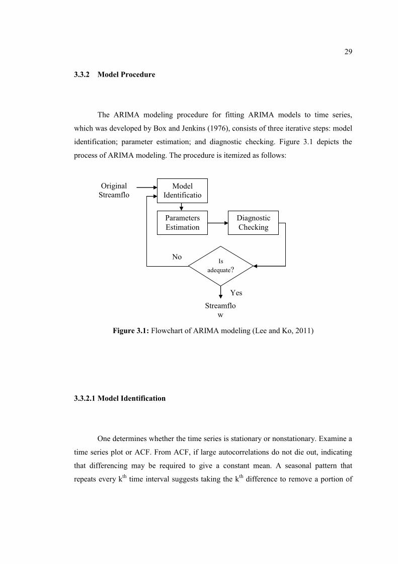
3.3.2 Model Procedure

The ARIMA modeling procedure for fitting ARIMA models to time series,

which was developed by Box and Jenkins (1976), consists of three iterative steps: model

identification; parameter estimation; and diagnostic checking. Figure 3.1 depicts the

process of ARIMA modeling. The procedure is itemized as follows:

Figure 3.1: Flowchart of ARIMA modeling (Lee and Ko, 2011)

3.3.2.1 Model Identification

One determines whether the time series is stationary or nonstationary. Examine a

time series plot or ACF. From ACF, if large autocorrelations do not die out, indicating

that differencing may be required to give a constant mean. A seasonal pattern that

repeats every kth time interval suggests taking the kth difference to remove a portion of

Streamflow

Model Identificatio

Parameters Estimation

Diagnostic Checking

Is adequate?

Original Streamflo

No

Yes

30

the pattern. Most series should not require more than two difference operations or

orders. Be careful not to overdifference. If spikes in the ACF die out rapidly, there is no

need for further differencing.

Next, examine the ACF and PACF of your stationary data in order to identify

what autoregressive or moving average models terms are suggested. Some general

guidelines (SPSS, 1993) using graphical method was applied in the identification

process:

i. Nonstationary series have an ACF that remains significant for half a dozen or

more lags, rather than quickly declining to 0. Difference must be done for such a

series until it is stationary before it can be identified.

ii. Autoregressive processes have an exponentially declining ACF and spikes in the

first one or more lags of the PACF. The number of spikes indicates the order of

the autoregression.

iii. Moving average processes have spikes in the first one or more lags of the ACF

and an exponentially declining PACF. The number of spikes indicates the order

of the moving average.

iv. Mixed (ARMA) processes typically show exponential declines in both the ACF

and the PACF.

At the identification stage, the sign of the ACF or PACF and the speed with which

an exponentially declining ACF or PACF approaches 0 are depend upon the sign and

actual value of the AR and MA coefficients (SSPS, 1993).

31

3.3.2.2 Parameter Estimation

Once the tentative model is formulated, the related model parameters are

estimated using the least squares scheme. Parameters are estimated to have zero gradient

of forecasting errors to the historical load data. The primary objective of this parameter

estimation is to minimize the forecasting error and determine both the model and its

parameters (Lee and Ko, 2011). Each ARIMA tentative model parameter can be tested

using t-values and p-values. Dividing the coefficient by its standard error calculates a t-

value.

3.3.2.3 Diagnostic Checking

Then, diagnostic test was conducted to ensure that the essential modeling

assumptions are satisfied for a given model. When the parameters have been well

estimated, the tentative model accuracy is validated by examining the ACF and PACF

residuals. The residuals should simulate the white noise process. Furthermore, the Q-

statistics test is applied to confirm the tentative model (O’Donovan, 1983). If the

calculated value Q exceeds the critical value of χ2 obtained from the chi-square tables,

the tentative model is inadequate (Lee and Ko, 2011).

Furthermore, for this stage, Ljung-Box is used for testing white noise residual.

Hypothesis null is that residual should be white noise. In other word, the residual series

should be independent, homoscedastic (having constant variance), and normally

distributed. We can reject hypothesis null if p-value in Chi-Square statistic greater than

alpha of 5%.

32

These steps are repeated until an adequate model is identified. When the steps in

ARIMA modeling are completed, a specific ARIMA model is applied to predict the

future monthly streamflow for 1 year ahead.

3.3.3 Minitab Procedures

For modeling ARIMA model, a statistical software has been uses, which is called

Minitab version 15. By using Minitab, ARIMA model step can be summarized as

follows:

1. Identify stationay of data

• If stationary, then go to step No. 3

• If non-stationary, then go to step No. 2

2. Apply the non-seasonal difference (d=1, k=1)

3. Identify seasonal pattern of the data using ACF

• If ACF indicating non-seasonal pattern, then go to step No. 5

• If ACF indicating seasonal pattern, then go to step No. 6

4. Identify general theoretical PACF of ARIMA model

5. Apply seasonal difference (D=1, k=12; D=2, k=24)

6. Identify general theoretical ACF and PACF of ARIMA model

• If seasonal pattern of ACF and PACF is still found from step No. 6, then go to

step No. 5

33

• If non-seasonal pattern of ACF is found then go to step No. 7

7. Apply the rest of procedures which are estimation, diagnostic check and

forecasting according to step No. 6until obtaining the best forecasting pattern.

3.4 Model Comparison and Forecast Evaluation Measures

In order to compare the forecasting accuracy of the different models, a

multicriterion performance evaluation procedure was used in this study. The following

indices were used to evaluate the performance of the models (Shalamu, 2009):

1. Mean Absolute Percentage Error (MAPE):

(3.7)

2. Root Mean Squared Error (RMSE):

(3.8)

3. Chi-Squared Test:

(3.9)

34

where,

Yi = the observed flow

Fi = the forecasted flow

CHAPTER 4

RESULT AND DISCUSSION

4.1 Introduction

This chapter consists of detail description on analysis of time series data using

both Markov and ARIMA modeling method for streamflow forecasting. Most of

computation work for ARIMA and Markov models are carried out by using Minitab

Microsoft Excel, respectively. Both of the methods will be used to model the streamflow

of Sungai Bernam at Tanjung Malim, Selangor (Station No. 3615412). The models will

be checked to get an adequate model for streamflow forecasting.

Data from January 1960 to December 2010 was used in deriving stochastic and

forecasting models. Data of 552 months from January 1960 to December 2005 are used

as calibration set for both model. Another 60 months data from January 2006 to

December 2010 is used as validation set.

36

4.2 Estimation of Missing Data Values

Some of data values are missing in the data series for Sungai Bernam

streamflow at Tanjung Malim (Station No. 3615412). In order to handle missing data for

this study, linear regression between flow of study area station and flow of adjacent

station is used. Regression line is determined as the best way to predict y from x. As

there was missing data of streamflow for Sungai Bernam at Tanjung Malim, streamflow

data of adjacent station at Jam. Skc (Station No. 3813411) is used. For example, there is

missing data of January 1962, February 1962 and March 1962. Some adjacent

observations month of streamflow data (previous and forward month) of both station are

used to get the regression line to estimate the missing data. This is shown in Figure 4.1.

Figure 4.1: Linear Regression of Two Streamflow Station for 1962

Missing month data of Station Tanjung Malim for January, February and March

1962 can be completed by using equation of linear regression y = 0.126x + 2.513 with

coefficient of determination, R2 of 0.845, which y and x represented flow of Station

Tanjung Malim (m3/s) and Jam. Skc (m3/s), respectively.

37

If data still cannot be obtained may be because the adjacent streamflow station

also had missing data for that month, rainfall data for adjacent station can be used to get

the regression equation to estimate the missing streamflow data. For example there is

missing data from February 1993 to May 1993 for both station of Tg. Malim and

Jam.Skc. Some adjacent observations month of rainfall data (previous and forward

month) of Station Ldg. Katoyang at Tg. Malim (Station No. 3714152) are used to get the

regression equation with flow data of Station Jam. Skc as shown in Figure 4.2. The

equation of the linear regression was found to be y = 0.146x + 10.43 with coefficient of

determination, R2 of 0.603, which y represented flow for Station Jam. Skc (m3/s) and x

represented rainfall for Station Ldg. Katayong (mm).

Figure 4.2: Linear Regression of Rainfall and Streamflow

After we know the streamflow data for February 1993 to May 1993 at Station

Jam. Skc, we can use that data to estimate the missing data of Station Tg. Malim from

the regression equation of both streamflow by using equation of linear regression y =

0.112x + 3.673 with coefficient of determination, R2 of 0.892, which y and x represented

flow of Station Tanjung Malim (m3/s) and Jam. Skc (m3/s), respectively. Figure 4.3

showed the regression line for the equation.

38

Figure 4.3: Linear Regression of Two Streamflow Station for 1993

After replacing all the missing data with appropriate estimation data from the

linear regression method, streamflow data of Sungai Bernam is shown in Appendix A.

4.3 Markov Model

Formulation of Markov Model is based on the procedures of data synthesis

which are: (1) determination of statistical parameters from the analysis of the historical

record, (2) identifying the frequency distribution of the historical data, (3) generating

random numbers of the same distribution and statistical characteristics and (4)

constituting the deterministic and combining with the random part.

39

4.3.1 Statistical Parameters of Historical Data

The sample mean flow for 612 month of data is 9.75 m3/s. Then, the sample

standard deviation, S is 4.66, skewness is 1.2, standard error is 0.18863 and coefficient

of variance is 0.47828. These statistical parameters can be calculated using Microsoft

Excel or can be obtained from EasyFit software. The result of the descriptive statistics

using EasyFit is shown in Figure 4.4.

Figure 4.4: Descriptive statistics of Sungai Bernam data

For data calibration, to model the streamflow, parameters of monthly historical

data from January 1960 to December 2005 which using 552 data is shown in Table 4.1.

40

Table 4.1: Parameters of Monthly Historical Data

i qj S2 Sj Rj Sj-1 bj qj-1

Jan 0.049549 9.07979E-05 0.009529 0.4442686 4.189053605 0.001 0.06 Feb 0.04537 8.89268E-05 0.00943 0.4901265 3.639813919 0.001 0.05 Mac 0.046522 9.69723E-05 0.009847 0.5777814 3.363576896 0.002 0.05 Apr 0.05187 9.10128E-05 0.00954 0.408 3.69337796 0.001 0.05 May 0.054888 5.21161E-05 0.007219 0.303 3.822355866 0.001 0.05 Jun 0.0488 6.94571E-05 0.008334 0.515 2.990121105 0.001 0.05 July 0.046073 7.22414E-05 0.008499 0.541 3.349038581 0.001 0.05 Aug 0.047227 7.71759E-05 0.008785 0.585 3.27283605 0.002 0.05 Sep 0.053852 7.21758E-05 0.008496 0.406 3.447681936 0.001 0.05 Oct 0.059644 7.62886E-05 0.008734 0.369 3.761513315 0.001 0.05 Nov 0.065038 6.89806E-05 0.008305 0.294 4.175448792 0.001 0.06 Dec 0.059643 0.000101211 0.01006 0.3699155 4.738293291 0.001 0.07

4.3.2 Identification of Distribution

In this study, statistical test is used for estimating the parameters of a probability

distribution. Kolmogorov-Smirnov (K-S) test, Anderson Darling (AD) test and Chi-

squared test can be used as statistical test. K-S test has being used as preference as it is

more powerful and robust. By using EasyFit application, the best-fitting distribution can

be found. K-S goodness of fit test for normal distribution is 0.13466 at ranking 42 while

for Lognormal distribution is 0.05954 at ranking 2. For AD goodness of fit test for

normal distribution is 139.43 at ranking 41 while for lognormal distribution is 34.169 at

ranking 6. Best-fitting distribution for the streamflow data of Sungai Bernam is

Lognormal Distribution (Figure 4.5 and Figure 4.6).

41

Histogram Inv. Gaussian (3P)

Flow, q (m3/s)30282624222018161412108642

0.3

0.28

0.26

0.24

0.22

0.2

0.18

0.16

0.14

0.12

0.1

0.08

0.06

0.04

0.02

0

Figure 4.5: Probability Density Function

Log-normal distribution is positively skewed, match with characteristic of many

hydrologic variables. This distribution is suitable for low-flow studies because small

changes in low values produce large changes in their logarithmic values.

42

Sample Inv. Gaussian (3P)

Flow, q (m3/s)30282624222018161412108642

1

0.9

0.8

0.7

0.6

0.5

0.4

0.3

0.2

0.1

0

Figure 4.6: Cumulative Distribution Function

As the distribution is log-normal, use the logarithm of the values and finally

convert back the flows. For an example, observed streamflow data in logarithmic values

for 1960 until 1970 is shown in Table 4.2, while other data for year (1971-2005) can be

found in Appendix B. These data as act calibration set to get the parameter of historical

data in order to model the future streamflow.

Table 4.2: Logarithmic Values of Observed Streamflow Data for 1960-1970 i Jan Feb Mac Apr May Jun Jul Aug Sep Oct Nov Dec

1960 0.056 0.051 0.058 0.064 0.055 0.046 0.057 0.049 0.058 0.057 0.063 0.065 1961 0.052 0.044 0.045 0.051 0.055 0.051 0.046 0.051 0.058 0.056 0.060 0.066 1962 0.059 0.046 0.056 0.057 0.055 0.046 0.045 0.049 0.056 0.069 0.075 0.058 1963 0.050 0.045 0.045 0.044 0.044 0.046 0.045 0.053 0.060 0.070 0.079 0.066 1964 0.056 0.047 0.050 0.052 0.056 0.045 0.057 0.048 0.060 0.058 0.065 0.064 1965 0.046 0.044 0.050 0.066 0.068 0.050 0.039 0.043 0.053 0.069 0.067 0.072 1966 0.058 0.048 0.052 0.058 0.045 0.052 0.053 0.054 0.057 0.072 0.077 0.072 1967 0.065 0.054 0.047 0.060 0.059 0.043 0.043 0.044 0.055 0.060 0.076 0.055 1968 0.040 0.037 0.031 0.041 0.059 0.050 0.043 0.043 0.055 0.057 0.058 0.060 1969 0.054 0.047 0.040 0.046 0.060 0.050 0.037 0.044 0.042 0.059 0.056 0.053 1970 0.054 0.034 0.036 0.045 0.052 0.038 0.043 0.045 0.054 0.055 0.058 0.061

43

4.3.3 Generation of Random Numbers

In this study, we generate random numbers using Microsoft Excel command

RAND( ). To get the random normal deviate, t, of mean equal to 1 and unit standard

deviation, we use inverse error function, erf-1(z):

(4.1)

Value of z can be obtained from cumulative distribution function (CDF) of the

log-normal distribution:

(4.2)

Figure 4.7: Cumulative distribution function of the log-normal distribution

44

(4.3)

As log-normal random numbers have both mean and standard deviation equal to

one. Therefore, the Equation 4.3 becomes:

(4.4)

If erf (x) = y, then erf -1 (y) = x. Let,

The value of t = ln x. Therefore,

(4.5)

As an example, the calculation procedure of random numbers generation for year

2006 is shown in Table 4.3, while the random numbers generation for other year (2007-

2010) can be found in Appendix C.

45

Table 4.3: Generation of Random Number for Year 2006

i RAND ( ) z erf -1 ti,j

January 0.699645 0.399289 0.370085 1.523379 February 0.45481 -0.090379 -0.08027 0.886483 March 0.063732 -0.872536 -1.0558 -0.49313 April 0.224711 -0.550577 -0.53482 0.243657 May 0.236038 -0.527923 -0.50847 0.280915 June 0.471912 -0.056176 -0.04983 0.929536 July 0.999341 0.998683 1.443813 3.041859

August 0.533139 0.066278 0.058805 1.083163 September 0.095672 -0.808656 -0.91763 -0.29772

October 0.044674 -0.910651 -1.15355 -0.63136 November 0.997494 0.994989 1.429319 3.021363 December 0.407816 -0.184368 -0.16487 0.766834

4.3.4 Streamflow Generation of Markov Model

As an example, the calculation deterministic part considering the persistence

(influence of previous flows) and combining with the random part to develop monthly

streamflow model for year 2006 is shown in Table 4.4, while the streamflow model for

other year (2007-2010) can be found in Appendix D.

The Markov model for monthly flows, developed by Thomas and Fiering is

using the following form (Maass et al., 1962):

(4.6)

46

We will use Equation 4.6 to develop Markov model for monthly flows. Flow in

ith month from the beginning, for jth month of the year can be modeled by adding mean

of flow of jth month of the year (January to December) with deterministic and random

component.

Table 4.4: Model Streamflow for Year 2006

i Deterministic Component Random Component Model flow

qi-1,j-1 qj+bj(qi-1,j-1-qj-1) ti,j Sjti,j√(1-rj2) qi,j (Log) qi,j (m3/s)

Jan 0.049549 0.049541669 1.523379 0.013 0.063 13.533 Febr 0.063 0.045386033 0.886483 0.007 0.053 9.077 Mac 0.053 0.04653475 -0.49313 -0.004 0.043 5.641 Apr 0.043 0.051865643 0.243657 0.002 0.054 9.604 May 0.054 0.054889433 0.280915 0.002 0.057 10.807 Jun 0.057 0.048803168 0.929536 0.007 0.055 10.210 Jul 0.055 0.046082272 3.041859 0.022 0.068 16.422

Aug 0.068 0.04726108 1.083163 0.008 0.055 10.014 Sep 0.055 0.053859993 -0.29772 -0.002 0.052 8.642 Oct 0.052 0.059642058 -0.63136 -0.005 0.055 9.821 Nov 0.055 0.065034911 3.021363 0.024 0.089 32.326 Dec 0.089 0.059661808 0.766834 0.007 0.067 15.849

4.3.5 Validation of Markov Model

The model streamflow by using Markov model is compared with the observed

streamflow that have been set as validation set for 60 monthly data from January 2006 to

December 2010. Graphically, from Figure 4.8, we can say that Markov model cannot

work well for streamflow forecasting for Sungai Bernam because it not match well with

the actual streamflow.

47

Figure 4.8: Comparison of Observed and Markov Model Flow

The ability of Markov model in streamflow forecasting is inspected by using

some forecast evaluation measures like Root Mean Square Error (RMSE), Chi-square

Test and Mean Absolute Percentage Error (MAPE). The result of inspection is

summarized in Table 4.5 and the details of the calculation can be found in Appendix E.

Table 4.5: Accuracy of the Markov Model

Performance Evaluation Procedure

Markov model

MAPE 53.66

RMSE 7.29

Chi-square test 250.99

48

4.4 ARIMA Model

In this study, an appropriate ARIMA tentative model for Sg. Bernam streamflow

is investigated. Examination of the autocorrelation function (ACF) and partial

autocorrelation function (PACF) provides a thorough basis for analyzing the system

behavior under time independence, and will suggest the appropriate parameters to

include in the model.

These tentative models will be checked and best tentative model will be selected

for streamflow forecasting of ARIMA model. As mentioned in previous chapter, the

ARIMA modeling follows three important stages that can be figured in flow diagram of

Box-Jenkins methodology (Figure 4.9).

Figure 4.9: Flow Diagram of Box-Jenkins Methodology

Ye

No

1. Tentative Identification

2. Parameter Estimation

3. Diagnostic Checking [Is the model adequate?]

4. Forecasting

-Testing parameters

- White noise of residuals - Normal distribution of residual

- Stationary & non- stationary time series - ACF & PACF

-Forecast calculation

49

4.4.1 Model Identification

Identification involve looking at the graph of sample autocorrelation function

(ACF) and sample partial autocorrelation function (PACF) to determine whether the

series is stationary or not and then make a decision what functional form best fits and

appropriate model for the data. In practice, the ACF and PACF are random variables and

will not give the same picture as the theoretical functions. This makes the model

identification more difficult and can involve much trial and error (Nazuha et al., 2010).

The most common method to check stationary is through examining the time

series plot of the data. Stationary means that data fluctuate around a constant mean. If

the time series plot is found to be non stationary, differencing needs to be applied.

Figure 4.10 showed that the data is non-stationary. The data need to be applied with non-

seasonal difference (d = 1, lag, k = 1). Based on graphical examination, Figure 4.11

showed that the data is stationary at the level of the data after applying non-seasonal

difference.

50

Year

Month2002199519881981197419671960JanJanJanJanJanJanJan

30

25

20

15

10

5

0

Stre

amflo

w, Y

t (m

3/s)

12

1110

9

8765

4321

12

11

10

9

8

7

6

5

4

321

12

11

10

9

876

5

432112

1110

9

876

54

32

1

12

11

10

9

876

5

4

32

1

12

11

1098

7

6

5

4

3

2

1

12

11

10

987

6

5

43

21

12

11

10

9

8

7654321

12

11

10

9

8

76

5

432

1

12

11

10

987

65

4

321

1211

109

8

7654

3

21

12

1110

9

8

7

654321

12

1110

9

8

76

54

32112

11

109876

5

4

321

12

1110

9

87

6

5

4

3

21

12

1110

9

876

5

432

1

12

11

10

9

8

76

54

3

2

1

12

11

10

9

87

6

5

432

1

12

11

10

9

8

7654

321

12

1110

9

876

5

4

32

1

12

11

10

9

876

5

4

321

12

11

10

987

65

432

1

1211

10

9

876

5

4321

12

11

10

98

7

6

54

321

12

11

10

9

87

6

54

3

21

12

11

10

98

7

65

4321

12

11

109

87654

32112

11

10

9

876

54

321

12

11

10

987

65

432

112

11

10

98

7

6

5432

1

12

11

10

9

8

7

6

543

211211

109876

54

32

1

12

1110

98

7

6

54

321

12

11

10

9

87

6

5

4321

12

11

10

9

8

76

54

3

2

1

1211109

876

5

4

32

1121110

98

7

6

5

4

3

2

1

1211109

87

6

5

4

321

12

11

10

9

876

54

3

2

1

12

11

10

9876

5

4

32

1

12

1110

9

87

6

54

3

21

1211

109

8

7

6

5432

1

12

11

10

9

8

765432

1

12

11

10

9

876

543

2

1

12

11109

8765

4

32

1

1211

109

8

7

6

5

4

3

2

1

Figure 4.10: Non stationary data of Sg. Bernam streamflow

YearMonth

2002199519881981197419671960JanJanJanJanJanJanJan

15

10

5

0

-5

-10

-15

Stre

amflo

w, d

1-Y

t (m

3/s)

1211

10

9

8

76

543

2

1

12

11

10

9

8

7

6

54

321

12

1110

9

87

6

54

321

12

11

10

987

6

5

4

3

2112

11

10

9

87

65

4

3

2

1

1211

109

8

76

54

3

21

12

11

1098

7

6

54

32

112

11

10

98

765432

1

12

11

109

8

7

6

5

4

3

2

1

12

11

10

9

8

7

6

5

4

32

1

12

11

10

9

8

76543

2

1

12

1110

9

8

7

65432

1

12

11

109

8

7

6

5

4

32

1

12

11

1098

7

6

54

321

12

11

10

9

8

76

5

43

2

1

12

11

10

9

87

6

5

43

21

12

11

109

8

7

6

5

4

3

21

12

11

10

9

8

7

65

43

2

112

11

10

98

7

6

54

32

112

11

10

9

8765

4

32

1

12

11

10

9

87

6

5

4

32

1

1211

1098

7

65

43

2

1

1211

10

9

87

6

5

4

3

2

1

12

11

1098

76

5

4

3

2

112

11

10

9

8

7

6

5

4

32

1

12

11

10

98

7

6

5

432

1

12

11

10

9

87654

32

1

12

11

109

87

6

54

32

11211

10

98

7

654

321

12

11

10

9

8

7

6

543

2

1

1211

10

9

8

7

6

54

3

211211

10

987

6

54

3

2

11211

10

9

8

76

5

4

32

1

12

11109

8

76

5432

1

12

11

10

98

76

5

4

3

2

1

121110

9

87

6

54

3

2

1

1211

10

9

8

76

5

4

321

121110

9

8

76

5

4

32

1

12

11

109

87

6

5

4

3

2112

11

10

9876

5

43

2

1

12

11

10

9

8

7

6

5

4

3

2

1

12

11

10

9

8

7

6

543

2

1

12

1110

98

76543

21

12

11

10

98

7

6

5

4

3

2

1

12

11

10

98

76

54

3

2

1

12

11

10

9

8

7

65

43

2

Figure 4.11: Stationary data of Sg. Bernam streamflow

The next step is to identify the values of p and q which are the AR (p) and MA

(q) components for both seasonal and non-seasonal series. For this purpose, the ACF and

51

PACF coefficient are computed. The following Table 4.6 gives general theoretical for

identification of the likely model:

Table 4.6: General Theoretical ACF and PACF of ARIMA models

Model ACF PACF MA(q): moving average of order q Cut off after lag q Dies down

AR(p): autoregressive of order p Dies down Cuts off after lag p

ARMA(p,q): mixed autoregressive-moving average of order (p,q)

Dies down Dies down

AR(p) or MA(q) Cuts off after lag q Cuts off after lag p

No order AR or MA (White Noise or Random process)

No spike No spike

65605550454035302520151051

1.0

0.8

0.6

0.4

0.2

0.0

-0.2

-0.4

-0.6

-0.8

-1.0

Lag

Aut

ocor

rela

tion

Autocorrelation Function for d1-Yt(with 5% significance limits for the autocorrelations)

Figure 4.12: ACF after non-seasonal difference

52

65605550454035302520151051

1.0

0.8

0.6

0.4

0.2

0.0

-0.2

-0.4

-0.6

-0.8

-1.0

Lag

Part

ial A

utoc

orre

lati

on

Partial Autocorrelation Function for d1-Yt(with 5% significance limits for the partial autocorrelations)

Figure 4.13: PACF after non-seasonal difference

As we can see from the Figure 4.12 and 4.13, ACF and PACF die down

gradually. Based on the pattern, the respective values of p, d, q was determined for

ARIMA is: ARIMA (1, 1, 1). From ACF correlogram, seasonal pattern of the data is

identified. As ACF is indicating seasonal pattern, seasonal difference (D = 1, lag, k =

12) needs to be applied.

65605550454035302520151051

1.0

0.8

0.6

0.4

0.2

0.0

-0.2

-0.4

-0.6

-0.8

-1.0

Lag

Aut

ocor

rela

tion

Autocorrelation Function for D1-d1-Yt(with 5% significance limits for the autocorrelations)

Figure 4.14: ACF after seasonal difference

53

65605550454035302520151051

1.0

0.8

0.6

0.4

0.2

0.0

-0.2

-0.4

-0.6

-0.8

-1.0

Lag

Part

ial A

utoc

orre

lati

on

Partial Autocorrelation Function for D1-d1-Yt(with 5% significance limits for the partial autocorrelations)

Figure 4.15: PACF after seasonal difference

After applying seasonal difference, we can see from the Figure 4.14, ACF cuts

off after lag 12 while in figure 4.15, PACF dies down. For seasonal ARIMA, the general

notation is ARIMA (p, d, q) (P, D, Q)S. Based on the pattern, the respective values of P,

D, Q was determined for ARIMA is: ARIMA (0, 1, 1)12. However, in order to make sure

that we have identified the right model, we suggest another tentative model which is

ARIMA (1, 1, 1)12.

4.4.2 Parameter estimation

Each ARIMA tentative model parameter can be tested using t-values and p-

values. Dividing the coefficient by its standard error calculates a t-value. The standard

error (SE) of coefficient is the standard deviation of the estimate of a regression

coefficient. It measures how precisely your data can estimate the coefficient’s unknown

value. Its value is always positive, and smaller values indicate a more precise estimate.

The standard error of a coefficient helps determine whether the value of the coefficient

54

is significantly different than zero. If the p-value associated with this t-statistic is less

than alpha level, we can conclude that the coefficient is significantly different from zero.

From Table 4.7, the standard error of MA 1 coefficient is large relative to the

value of the coefficient itself, so the t-value of 1.26 is too small to declare statistical

significance. We reject hypothesis null if |t|> tα/2,df = n-np. For MA 1 parameter, tcalc

(=1.26) < ttable (=2.25). The resulting p-value also is much greater than common alpha

level. Therefore, hypothesis null cannot be rejected. So we can conclude this coefficient

not differs from zero. Table 4.8 which estimates parameters for ARIMA (1,1,1)(0,1,1)12

have |tcalc|> ttable (= 2.25) and p-value is less than alpha level. Hence, hypothesis null can

be rejected, and we can conclude that the coefficient is significantly different from zero.

Table 4.7: Final Estimates of Parameters for ARIMA (1,1,1)(1,1,1)12

Type Coefficient SE Coefficient T p

AR 1 0.2782 0.0520 5.35 0.000

SAR 12 0.0589 0.0467 1.26 0.208

MA 1 0.8765 0.0256 34.24 0.000

SMA 12 0.9537 0.0206 46.25 0.000

Table 4.8: Final Estimates of Parameters for ARIMA (1,1,1)(0,1,1)12

Type Coefficient SE Coefficient T p

AR 1 0.2894 0.0516 5.61 0.000

MA 1 0.8788 0.0248 35.41 0.000

SMA 12 0.9553 0.0184 51.98 0.000

55

4.4.3 Diagnostic Checking

The next step of model identification method of time series modeling approach is

diagnostic checking. It is aimed at examining the accuracy of the chosen tentative model

in ensuring that the modeling assumptions are satisfied. Several procedures can be

applied to check the adequacy of the model as to whether the model satisfies the stability

or stationary condition, as required in stochastic modeling works (Ayob and Amat,

2004).

For this stage, Ljung-Box is used for testing white noise residual. Hypothesis

null is that residual should be white noise. In other word, the residual series should be

independent, homoscedastic (having constant variance), and normally distributed. We

can reject hypothesis null if p-value in Chi-Square statistic greater than alpha of 5%.

In this study, both ARIMA tentative models have p-value less than alpha level.

Table 4.9 and Table 4.10 showed p-value for both tentative models. So, the hypothesis

null cannot be rejected and we can conclude that residual is significantly white noise for

both tentative models.

Table 4.9: Modified Box-Pierce (Ljung-Box) Chi-Square statistic

for ARIMA (1,1,1)(1,1,1)12

Lag 12 24 36 48

Chi-Square 21.2 61.8 82.7 98.1

DF 8 20 32 44

p-Value 0.007 0.000 0.000 0.000

56

Table 4.10: Modified Box-Pierce (Ljung-Box) Chi-Square statistic

for ARIMA (1,1,1)(0,1,1)12

Lag 12 24 36 48

Chi-Square 23.1 62.2 82.7 97.9

DF 9 21 33 45

p-Value 0.006 0.000 0.000 0.000

Besides that, the best tentative model can be determined through test of Least

Square Error (LSE) and Root Mean Square Error (RMSE). The result for the test on the

tentative model is summarized in Table 4.11. The best fit in the least-squares sense

minimizes the sum of squared residuals, a residual being the difference between an

observed value and the fitted value provided by a model. RMSE also is a good measure

of accuracy. The smaller the value of LSE and RMSE, the tentative model is more

accurate.

Table 4.11: LSE and RMSE Test for ARIMA Tentative Model

Test ARIMA

(1,1,1)(1,1,1)12

ARIMA

(1,1,1)(0,1,1)12

Least Square Error (LSE) 1798 1760

Root Mean Square Error (RMSE) 5.5 5.4

So, from two tentative models possible, the model that best fits the criteria and

meets the requirement is model ARIMA (1,1,1)(0,1,1)12. Forecasting is made based on

the chosen model. The model we identified as best-fit model for Sg. Bernam streamflow

is:

(1 - φ1B)(1-B)(1-B12)Yt = (1- θ1B)(1- θ2B12)at (4.7)

57

Rewriting the model, we have the following:

(1 - φ1B)(1-B12-B+B13)Yt = (1- θ2B12- θ1B + θ1θ2B13)at

(1 - φ1B)(1-B12-B+B13)Yt = (1- θ2B12- θ1B + θ1θ2B13)at

(1-B12-B+B13- φ1B+ φ1B13+ φ1B2- φ1B14) Yt = (1- θ2B12- θ1B + θ1θ2B13)at

(1 - B12 – (1+ φ1)B + (1+ φ1)B13 + φ1B2 - φ1B14) Yt = (1- θ1B - θ2B12 + θ1θ2B13)at

Yt – (1+ φ1)Yt-1 + φ1Yt-2 – Yt-12 + (1+ φ1)Yt-13 - φ1Yt-14 = at - θ1at-1 – θ2at-12 + θ1θ2at-13

Yt = (1+ φ1)Yt-1 - φ1Yt-2 + Yt-12 - (1+ φ1)Yt-13 + φ1Yt-14 + at - θ1at-1 – θ2at-12 + θ1θ2at-13

Noted that,

AR1, φ1 = 0.2894

MA1, θ1 = 0.8788

SMA 12 θ2 = 0.9553

Yt = (1+ 0.2894) Yt-1 – 0.2894Yt-2 + Yt-12 - (1+ 0.2894) Yt-13 + 0.2894Yt-14 + 0.2894Yt-14

+ at – 0.8788at-1 – 0.8788at-12 + (0.8788x0.9553)at-13

Yt = 1.2894 Yt-1 – 0.2894Yt-2 + Yt-12 - 1.2894Yt-13 + 0.2894Yt-14 +

at – 0.8788at-1 – 0.9553at-12 + 0.8395at-13

Yt = Yt-12 + [1.2894 Yt-1 - 1.2894Yt-13 - 0.2894Yt-2 + 0.2894Yt-14] +

[at – 0.8788at-1 – 0.9553at-12 + 0.8395at-13] (4.8)

Equation (4.8) can be used for streamflow forecasting of ARIMA model. From

Equation 4.8 also, its explained that the forecast for time period t is the sum of (1) the

value of the time series in the same month of the previous year, (2) a trend component

determined by the difference of previous month’s value and last year’s previous month’s

value and difference of last year’s previous two month’s value and previous two month’s

value; (3) the effects of random shocks (or residuals) of period t, t-1, t-12 and t-13 on the

forecast.

58

4.4.4 Streamflow Generation of ARIMA Model

In this study, we will use Minitab to develop Markov model for monthly flows.

As an example, develop monthly streamflow model using Minitab for year 2006 to 2007

is shown in Table 4.12, while the streamflow model for other year (2008-2010) can be

found in Appendix F.

Table 4.12: Model Streamflow for Year 2006-2007

i Actual Flow (m3/s)

Model Flow (m3/s) Residual Fit Coefficient

Jan 2006 13.08 9.6732 * * 0.289364 Feb 2006 8.12 7.1884 * * 0.878761 Mac 2006 6.11 7.2612 * * 0.955283 Apr 2006 29.72 9.0165 * * May 2006 29.22 9.9281 * * Jun 2006 17.82 7.6110 * * Jul 2006 7.94 6.7046 * *

Aug 2006 9.95 7.0851 * * Sep 2006 28.05 9.5168 * * Oct 2006 17.63 12.2889 * * Nov 2006 17.72 15.2005 * * Dec 2006 11.23 12.3581 * * Jan 2007 9.05 7.9227 * * Feb 2007 6.80 6.6970 -1.57988 7.5299 Mac 2007 7.62 7.1341 -1.39072 7.6507 Apr 2007 13.46 8.9949 -1.05700 9.4570 May 2007 12.05 9.9369 -0.14946 10.2195 Jun 2007 11.38 7.6286 1.10867 7.3913 Jul 2007 13.06 6.7248 -1.04180 7.8818

Aug 2007 8.95 7.1060 1.04920 7.2208 Sep 2007 9.36 9.5379 0.26505 11.0050 Oct 2007 14.33 12.3101 -2.99026 13.4603 Nov 2007 14.26 15.2217 -3.58500 15.6250 Dec 2007 8.24 12.3794 4.03841 11.4816

59

4.4.5 Validation of ARIMA Model

The model streamflow by using ARIMA model is compared with the observed

streamflow that have been set as validation set for 60 monthly data from January 2006 to

December 2010. Graphically, from Figure 4.16, we can say that ARIMA model may

works quite well for streamflow forecasting for Sungai Bernam because many data from

model match well with the actual streamflow. The ability of ARIMA model in

streamflow forecasting is inspected using some forecast evaluation measures.

Figure 4.16: Comparison Observed and ARIMA Model Flow

Like in Markov model’s validation, the forecast evaluation measures like Root

Mean Square Error (RMSE), Chi-square Test and Mean Absolute Percentage Error

60

(MAPE) are used to examine the accuracy of ARIMA model. The result of inspection is

summarized in Table 4.13 and the details of the calculation can be found in Appendix G.

Table 4.13: Accuracy of the ARIMA Model

Performance Evaluation Procedure

ARIMA model

MAPE 27.50

RMSE 5.41

Chi-square test 191.11

4.5 Model Comparison and Forecast Evaluation Measures

Streamflow forecasting methods of Markov model is being compared with

ARIMA model to inspect the accuracy between the models in forecasting ability.

Observed streamflow data that have been set as validation set for 60 monthly data from

January 2006 to December 2010 is used as bench mark to make the comparison. From

From graphical examination on Figure 4.17, we can say that ARIMA model is better for

streamflow forecasting for Sungai Bernam because more data from ARIMA model

match with the actual streamflow.

Most of streamflow forecast by Markov model has higher streamflow value

rather than the actual data. In the accuracy aspects, Markov model is not good rather

than ARIMA model because the model cannot obtain the exact or similar pattern with

the actual ones. However, these high values are a good forecasting as a reference

guideline to prevent damage due to flood problem. We can use Markov model for short-

61

term forecasting, like hourly and daily forecasting in order to give more accurate flood

warning.

Meanwhile, if the forecasts streamflow has the lower value from the actual data,

we cannot estimate the flood occurrence. Lower streamflow forecasts is needed in some

of agriculture field to make sure that plants have sufficient water and grow well.

Figure 4.17: Model Comparison

For short period, ARIMA model can obtain the exact or similar pattern with the

actual ones. ARIMA cannot forecast accurately for longer period as it is best used for

short-term forecasting. Usually, it will tend to become flat for sufficiently long period.

Actually, ARIMA model which is good at short-term forecasting can also be used to

control flood.

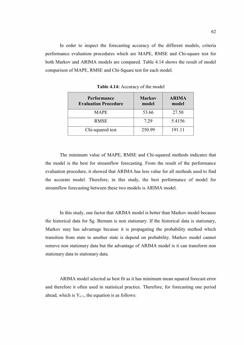
62

In order to inspect the forecasting accuracy of the different models, criteria

performance evaluation procedures which are MAPE, RMSE and Chi-square test for

both Markov and ARIMA models are compared. Table 4.14 shows the result of model

comparison of MAPE, RMSE and Chi-Square test for each model.

Table 4.14: Accuracy of the model

Performance Evaluation Procedure

Markov model

ARIMA model

MAPE 53.66 27.50

RMSE 7.29 5.4156

Chi-squared test 250.99 191.11

The minimum value of MAPE, RMSE and Chi-squared methods indicates that

the model is the best for streamflow forecasting. From the result of the performance

evaluation procedure, it showed that ARIMA has less value for all methods used to find

the accurate model. Therefore, in this study, the best performance of model for

streamflow forecasting between these two models is ARIMA model.

In this study, one factor that ARIMA model is better than Markov model because

the historical data for Sg. Bernam is non stationary. If the historical data is stationary,

Markov may has advantage because it is propagating the probability method which

transition from state to another state is depend on probability. Markov model cannot

remove non stationary data but the advantage of ARIMA model is it can transform non

stationary data to stationary data.

ARIMA model selected as best fit as it has minimum mean squared forecast error

and therefore it often used in statistical practice. Therefore, for forecasting one period

ahead, which is Yt+1, the equation is as follows:

63

Yt+1 = Yt-11 + [1.2894 Yt - 1.2894Yt-12 - 0.2894Yt-1 + 0.2894Yt-13] +

[at+1 – 0.8788at – 0.9553at-11 + 0.8395at-12] (4.9)

By using Minitab, we can easily do streamflow forecasting for the future values

of time series from current and past values. Figure 4.18 shows the comparison of pattern

of streamflow for actual and model streamflow for Sungai Bernam. The first 5 years

from Jan 2006 to December 2010 is the calibration process. This time series plot reveal

pattern of cycles of ARIMA model. We can see that, the model flows follow the pattern

of observed streamflow quite well although the data is nonstationary for several years.

YearMonth

2015201420132012201120102009200820072006JanJanJanJanJanJanJanJanJanJan

30

25

20

15

10

5

Stre

amflo

w, Y

t (m

3/s)

Yt-actualYt-model

Variable

12

11

109876

54

32

112

11

10

9876

5

43

2112

11

10

9

8

76

5

4

3

2

1

12

1110

98

7

654

32

1

12

1110

9

8

7

6

54

3

2

1 12

11

10

9

876

54

321

12

11

10

9

876

54

321

12

11

10

9

876

54

321

12

11

10

9

876

54

321

12

11

10

9

876

54

321

12

11

10

9

876

54

321

12

11

10

9

876

54

321

12

11

10

9

876

54

321

12

11

10

9

876

54

321

12

11

10

9

876

54

32

1

Figure 4.18: Streamflow for actual and model

The next 5 years is the forecast streamflow using ARIMA model which is 60

months from January 2011 to December 2015. We can see from the figure, the model

64

can forecast well but the pattern of streamflow is repeated the same pattern for longer

period. This is because ARIMA model is only good and best suited for short term

forecasting since its forecast on previous observations. For short term forecasting, Box-

Jenkins model can nicely reproduce the details of the original series. ARIMA cannot

forecast accurately for longer period.

CHAPTER 5

CONCLUSION AND RECOMMENDATIONS

4.1 Conclusion

This study has fulfilled the objectives of the study to propose the streamflow

forecasting methods using Markov and ARIMA models and then inspect the accuracy of

both models in forecasting ability. The Box-Jenkins or ARIMA model is one of the most

popular time series forecasting methods. Markov model has its own advantage in

forecasting ability.

In this study, the tentative model that best fits the criteria and meets the

requirement is model ARIMA (1,1,1)(0,1,1)12. By analyzing the forecasted value using

the performance evaluation procedure, it is found that use of ARIMA model for

forecasting Sg. Bernam streamflow is better than Markov model. From the result of the

performance evaluation procedure, it showed that ARIMA has less value for all methods

used. Therefore, ARIMA model has the ability to predict accurately the future monthly

streamflow for Sungai Bernam.

66

The critical part in modeling using ARIMA is identification of best tentative

model. The tentative model that has been identified will be tested and checked to clarify

that the model is the best fit.

Markov also has some advantage because it forecasts with higher streamflow

compare to actual streamflow. Higher streamflow can cause disaster like flood.

Therefore, Markov model can be used for flood control.

Both Markov and ARIMA models are good for short term forecasting. From the

result, we can see that both models can forecast well for earlier period. But, for longer

period, they cannot forecast accurately.

Although both models good for short-term forecasting and not good for long-

term forecasting, comparison between the two model shows that ARIMA is better in

giving accurate forecasts.

4.2 Recommendations

Based on the result, both Markov and ARIMA model can be used for streamflow

forecasting. However, there are some weaknesses that can be overcome. Here are some

recommendations that can be used to increase the accuracy for streamflow forecasting:

67

1. The amount of data, or equivalently the number of training patterns also affects

the forecast performance. For long memory series, more training patterns results

in more accurate forecasts. To forecast accurately, use long input series.

2. To control flood efficiently, we can use Markov model for short-term forecasting

because short-term forecasting is very useful for control flood.

3. Use ARIMA model for short-term forecasting only including for streamflow

forecasting.

4. Compare the streamflow forecasting with other forecasting methods of time

series such as exponential smoothing, regression analysis or Fourier series

analysis.

5. Do the forecasting time series after removing the outliers.

6. Use hybrid model using ARIMA and artificial neural network in streamflow

forecasting.

68

REFERENCES

Adib, A. and Majd, A. R. M. (2009). Optimization of Reservoir Volume by Yield Model

And Simulation of it by Dynamic Programming and Markov Chain Method.

American-Eurasion J. Agric. & Environ. Sci., 5(6), 796-803.

Akgun, B. (2003). Identification of Periodic Autoregressive Moving Average Models.

Middle East Technical University.

Ayob, K. and Amat, S. D. (2004). Water Use Trend at Universiti Tekologi Malaysia:

Application of Arima Model. Jurnal Teknology, 41 (B): 47-56

Bell, W. R. (1984). An Introduction to Forecasting with Time Series Models. Insurance:

Mathematics and Economics 3, pp. 241-255.

Bowerman, B. L. and O’Connell, R. T. (1993). Forecasting and Time Series: An

Applied Approach. Third Edition. Duxbury Press.

Box, G. E. P. and Jenkins, G. M. (1970). Time Series Analysis: Forecasting and Control.

Holden Day, San Francisco.

Box, G. E. P. and Jenkins, G. M. (1976). Time Series Analysis, Forecasting and Control.

Holden Day, San Francisco.

Box, G. E. P., Jenkins, G. M. and Reinsel, G. C. (1994). Time Series Analysis:

Forecasting and Control. Third Edition. Prentice Hall.

Brown, R. G. (1962). Smoothing, Forecasting and Prediction of Discrete Time Series.

Prentice Hall, Englewood Cliffs, N. J.

69

Dalphin, R. J. (1987). Markov-Weibull Model of Monthly Streamflow. Journal of Water

Resources Planning and Management, Vol. 113, No. 1.

Fiering, M. B., and Jackson, B. B. (1971). Synthetic Streamflows. Water Resources

Monograph 1. American Geophysicists Union. Washington, D. C.

Fortin, V., Perreault, L. and Salas, J. D. (2004). Retrospective Analysis and Forecasting

of Streamflows Using a Shifting Model. Journal of Hydrology, Vol. 296,

135-163.

Gupta, R. S. (1989). Hydrology and Hydraulic Systems. Prentice Hall, pp 343-350.

Hasmida, H. (2009). Water Quality Trend at The Upper Part of Johor River in Relation

to Rainfall and Runoff Pattern. Universiti Teknologi Malaysia.

Heiko, B. (2000). Markov Chain Model for Vegetation Dynamics. Ecological Modeling,

Vol. 126, pp. 139-154.

Hendranata, A. (2003). ARIMA (Autoregressive Moving Average). Manajemen

Keuangan Sektor Publik FEUI

Ho, S. L. and Xie, M. (1998). The Use of ARIMA Models for Reliability Forecasting

and Analysis. Computers ind. Engng, Vol. 35, Nos 1-2, pp. 213-216.

Joomizan, N. (2010). Reservoir Storage Simulation and Forecasting Models for Muda

Irrigation Scheme, Malaysia. Universiti Teknologi Malaysia.

Lee, C. and Ko, C. (2011). Short-term Load Forecasting Using Lifting Scheme and

ARIMA Models. Expert Systems with Applications, Vol. 38, pp. 5902-5911.

Leemis, L. (1998). Input Modeling. In Proceedings of the 1998 Winter Simulation

70

Conference, ed. D. J. Medeiros, E. F. Watson, J. S. Carson, and M. S.

Manivannan, 15–22. Piscataway, New Jersey: Institute of Electrical and

Electronics Engineers, Inc.

Maass, A., Hufschmidt, M. M., Dorfman, R., Thomas, H. A., Marglin, S. A., Fair and G.

M. (1962). The Design of Water-Resource Systems. Harvard University Press,

Cambridge, Mass., pp 467

Maia, A. L. S., de Carvalho, F. de A. T. and Ludermir, T. B. (2008). Forecasting Models

for Interval-valued Time Series. Neurocomputing, Vol. 71, pp. 3344-3352.

Modarres, R. (2007). Streamflow Drought Time Series Forecasting. Stoch Environ Res

Risk Assess.

Mohd Shafiek, Y. Hishamuddin, J. and Sobri, H. (2005). Daily Streamflow Forecasting

Using Simplified Rule-Based Fuzzy Logic System. Journal-The Institution of

Engineers, Malaysia, Vol. 66, No. 4.

Montgomery, D. C., Jennings, C. L., Kulahci, M. (2008). Introduction to Time Series

Analysis and Forecasting. John Wiley & Sons, Inc.

Moore, D. S. and McCabe, G. P. (1999). Introduction to the Practice of Statistics. Third

Edition. New York: W. H. Freeman.

Naadimuthu, G. and Lee, E. S. (1982). Stochastic Modelling and Optimization of Water

Resources Systems. Mathematical Modelling, Vol. 3, pp. 117-136.

Nazuha, M., Ruzaidah, S. and Zamzulani, M. (2010). Malaysia Crude Oil Production

Estimation: an Application of ARIMA Model. International Conference on

Science and Social Research (CSSR 2010)

71

O’Donovan, T. M. (1983). Short Term Forecasting: An Introduction to the Box-Jenkins

Approach. New York: Wiley.

Shalamu, A. (2009). Monthly and Seasonal Streamflow Forecasting in the Rio Grande

Basin. New Mexico State University

Shunway, R. H. (1988). Applied Statistical Time Series Analysis. Prentice Hall,

Englewood Cliffs, New Jersey.

SPSS (1993). SPSS for Windows-Trend. Release 6.0.

Tang, Z., Almeida, C. and Fishwick, P. A. (1991). Time Series Forecasting Using

Neural Networks vs. Box-Jenkins Methodology. Simulation.

Wang, W. (2006). Stochasticity, Nonlinearity and Forecasting of Streamflow Processes.

IOS Press, Amsterdam.

Wurbs, R. A. (2005). Comparative Evaluation of Generalized River/Reservoir Systems

Models. Texas Water Resources Institute, TR-282, pp. 27-131.

Yafee, R. and McGee, M. (2000). Introduction to Time Series Analysis and Forecasting

with Application of SAS and SPSS. Academic Press, Inc., New York.

Yurekli, K., Kurunc, A. and Simyek, H. (2004). Prediction of Daily Maximum

Streamflow Based on Stochastic Approaches. Journal of Spatial Hydrology,

Vol.4.

72

APPENDIX A

Streamflow Data of Sungai Bernam 1960-2010 i Jan Feb Mac Apr May Jun Jul Aug Sep Oct Nov Dec

1960 10.62 8.38 11.23 14.08 10.04 6.68 11.01 7.87 11.11 10.83 13.83 14.62 1961 8.72 5.95 6.26 8.40 10.07 8.50 6.84 8.27 11.27 10.47 12.04 15.52 1962 11.98 6.66 10.28 11.06 10.07 6.62 6.36 7.79 10.54 16.97 21.14 11.29 1963 8.06 6.35 6.37 6.02 6.20 6.76 6.45 9.29 12.09 17.82 23.87 15.37 1964 10.31 7.08 7.90 8.73 10.35 6.44 11.09 7.52 12.39 11.24 14.58 14.11 1965 6.65 6.12 7.96 15.45 16.39 8.23 4.64 5.81 9.32 16.98 15.76 18.94 1966 11.41 7.38 8.96 11.25 6.45 8.70 9.38 9.49 11.04 19.17 22.08 18.80 1967 14.99 9.69 6.91 12.13 11.64 5.89 5.79 5.94 9.91 12.40 21.74 9.84 1968 4.87 4.12 2.94 5.14 11.72 8.16 5.64 5.91 9.91 11.05 11.56 12.16 1969 9.61 6.95 4.83 6.75 12.50 8.24 4.26 6.21 5.52 11.84 10.30 9.08 1970 9.69 3.49 3.83 6.48 8.71 4.41 5.73 6.49 9.79 9.96 11.16 12.61 1971 17.40 6.48 8.20 5.99 7.06 5.06 4.77 8.17 11.53 6.94 14.11 18.31 1972 8.09 8.04 7.84 9.31 11.60 9.16 5.88 5.75 8.74 11.88 16.21 9.22 1973 6.27 5.26 5.29 9.88 11.09 8.87 5.04 7.74 7.42 10.81 9.60 7.13 1974 3.62 7.44 6.80 8.65 9.52 7.24 7.54 7.79 8.43 7.11 8.15 8.68 1975 8.49 7.38 10.91 11.46 11.50 8.29 10.70 6.90 11.33 6.14 10.71 13.69 1976 7.88 4.36 5.59 6.05 4.92 7.92 5.94 8.74 7.55 14.43 12.72 7.66 1977 6.84 4.90 3.34 3.80 5.61 6.51 4.10 3.73 4.38 18.96 13.17 8.54 1978 5.14 3.54 3.36 6.39 7.93 3.67 3.99 2.99 4.72 7.86 20.75 5.60 1979 4.08 4.33 3.87 5.70 5.86 5.24 5.30 5.01 8.86 7.79 12.88 6.31 1980 4.05 3.95 4.91 5.01 10.07 9.37 6.51 8.79 9.64 12.48 8.48 19.07 1981 8.07 6.99 4.38 10.73 11.90 7.37 4.83 4.62 9.23 7.44 15.02 10.03 1982 4.95 3.93 5.26 8.94 9.40 6.94 4.84 6.55 7.73 10.01 18.93 8.03 1983 4.02 2.47 3.84 3.18 5.42 3.65 4.39 5.68 10.02 5.57 7.60 8.18 1984 5.86 9.04 8.07 8.10 9.83 9.93 5.98 5.07 5.64 7.82 14.58 19.78 1985 9.55 8.80 9.26 6.99 11.31 5.53 5.34 4.85 7.14 12.75 21.16 15.96 1986 7.95 5.79 4.94 8.87 6.31 4.32 3.21 3.68 7.39 14.19 13.57 8.74 1987 4.38 4.07 3.76 5.67 6.03 4.51 4.75 9.03 12.35 18.64 12.26 9.13 1988 4.81 7.86 6.48 6.22 9.92 12.09 8.45 8.57 18.19 9.24 11.01 7.39 1989 4.56 2.91 6.13 11.96 11.79 8.73 8.27 5.09 8.02 12.06 17.90 9.49 1990 5.80 3.14 2.65 3.46 10.15 5.94 4.55 3.31 6.83 16.42 15.36 11.83 1991 3.89 3.51 5.83 7.66 11.97 9.24 5.59 5.09 7.83 13.20 13.55 8.27 1992 7.37 6.28 5.56 7.18 9.65 5.64 6.94 6.01 6.43 7.65 12.25 8.49 1993 7.10 8.00 7.56 11.41 12.62 7.69 8.96 6.15 9.60 12.40 12.87 16.91 1994 10.66 10.16 10.32 10.59 10.87 10.78 8.43 10.89 16.08 14.22 13.97 16.15 1995 10.85 9.37 11.74 13.89 14.36 14.15 13.34 16.59 12.99 13.99 17.08 16.12 1996 12.29 11.50 12.12 18.45 15.91 16.73 13.12 14.24 13.39 20.88 17.08 29.78 1997 16.24 19.71 20.96 20.22 17.51 20.14 19.05 15.69 18.91 21.15 26.92 18.46 1998 15.95 16.02 14.69 14.42 14.90 15.72 16.14 20.16 23.75 19.72 27.30 18.59 1999 9.18 9.77 11.69 11.82 13.56 9.54 7.52 8.99 10.50 13.37 11.77 16.19 2000 14.05 11.67 15.70 12.87 9.26 7.45 4.21 9.25 8.85 9.31 14.58 19.88 2001 13.58 9.33 8.05 13.36 10.84 7.30 5.72 5.05 8.66 6.43 10.47 7.83 2002 6.04 4.35 4.84 11.45 12.75 7.89 6.99 7.26 8.96 15.31 16.94 7.30 2003 7.45 6.91 5.85 7.34 9.23 6.69 7.32 6.71 8.80 13.25 19.15 9.72 2004 8.08 6.60 6.67 8.68 11.12 4.13 6.49 4.44 11.62 14.57 21.65 8.07 2005 3.87 2.73 4.38 4.51 6.26 6.07 4.56 5.63 3.53 14.99 16.39 18.46 2006 13.08 8.12 6.11 29.72 29.22 17.82 7.94 9.95 28.05 17.63 17.72 11.23 2007 9.05 6.80 7.62 13.46 12.05 11.38 13.06 8.95 9.36 14.33 14.26 8.24 2008 11.29 6.76 9.58 12.86 9.73 12.28 10.89 7.83 9.85 13.14 16.74 10.96 2009 9.73 9.67 15.10 13.72 8.75 7.31 8.05 9.03 10.08 7.99 12.73 6.88 2010 6.83 4.86 4.36 7.18 6.17 7.51 7.45 8.04 7.16 6.30 9.56 11.01

73

APPENDIX B

Logarithm of Observed Streamflow Data for 1960-2005 i Jan Feb Mac Apr May Jun Jul Aug Sep Oct Nov Dec

1960 0.056 0.051 0.058 0.064 0.055 0.046 0.057 0.049 0.058 0.057 0.063 0.065 1961 0.052 0.044 0.045 0.051 0.055 0.051 0.046 0.051 0.058 0.056 0.060 0.066 1962 0.059 0.046 0.056 0.057 0.055 0.046 0.045 0.049 0.056 0.069 0.075 0.058 1963 0.050 0.045 0.045 0.044 0.044 0.046 0.045 0.053 0.060 0.070 0.079 0.066 1964 0.056 0.047 0.050 0.052 0.056 0.045 0.057 0.048 0.060 0.058 0.065 0.064 1965 0.046 0.044 0.050 0.066 0.068 0.050 0.039 0.043 0.053 0.069 0.067 0.072 1966 0.058 0.048 0.052 0.058 0.045 0.052 0.053 0.054 0.057 0.072 0.077 0.072 1967 0.065 0.054 0.047 0.060 0.059 0.043 0.043 0.044 0.055 0.060 0.076 0.055 1968 0.040 0.037 0.031 0.041 0.059 0.050 0.043 0.043 0.055 0.057 0.058 0.060 1969 0.054 0.047 0.040 0.046 0.060 0.050 0.037 0.044 0.042 0.059 0.056 0.053 1970 0.054 0.034 0.036 0.045 0.052 0.038 0.043 0.045 0.054 0.055 0.058 0.061 1971 0.069 0.045 0.050 0.044 0.047 0.041 0.039 0.050 0.058 0.047 0.064 0.071 1972 0.050 0.050 0.049 0.053 0.059 0.053 0.043 0.043 0.052 0.059 0.067 0.053 1973 0.045 0.041 0.041 0.055 0.057 0.052 0.040 0.049 0.048 0.057 0.054 0.047 1974 0.035 0.048 0.046 0.052 0.054 0.048 0.049 0.049 0.051 0.047 0.050 0.052 1975 0.051 0.048 0.057 0.058 0.058 0.051 0.057 0.047 0.058 0.044 0.057 0.063 1976 0.049 0.038 0.042 0.044 0.040 0.050 0.044 0.052 0.049 0.064 0.061 0.049 1977 0.046 0.040 0.033 0.035 0.042 0.045 0.037 0.035 0.038 0.072 0.062 0.051 1978 0.041 0.034 0.033 0.045 0.050 0.035 0.036 0.032 0.039 0.049 0.075 0.042 1979 0.037 0.038 0.036 0.043 0.043 0.041 0.041 0.040 0.052 0.049 0.061 0.045 1980 0.037 0.036 0.040 0.040 0.055 0.053 0.045 0.052 0.054 0.060 0.051 0.072 1981 0.050 0.047 0.038 0.057 0.059 0.048 0.040 0.039 0.053 0.048 0.065 0.055 1982 0.040 0.036 0.041 0.052 0.053 0.047 0.040 0.046 0.049 0.055 0.072 0.050 1983 0.036 0.029 0.036 0.033 0.042 0.035 0.038 0.043 0.055 0.042 0.049 0.050 1984 0.043 0.053 0.050 0.050 0.055 0.055 0.044 0.041 0.043 0.049 0.065 0.073 1985 0.054 0.052 0.053 0.047 0.058 0.042 0.042 0.040 0.047 0.061 0.075 0.067 1986 0.050 0.043 0.040 0.052 0.045 0.038 0.033 0.035 0.048 0.064 0.063 0.052 1987 0.038 0.037 0.035 0.043 0.044 0.038 0.039 0.053 0.060 0.071 0.060 0.053 1988 0.040 0.049 0.045 0.045 0.055 0.060 0.051 0.051 0.071 0.053 0.057 0.048 1989 0.039 0.031 0.044 0.059 0.059 0.052 0.051 0.041 0.050 0.060 0.070 0.054 1990 0.043 0.032 0.030 0.034 0.055 0.044 0.039 0.033 0.046 0.068 0.066 0.059 1991 0.036 0.034 0.043 0.049 0.059 0.053 0.042 0.041 0.049 0.062 0.063 0.051 1992 0.048 0.045 0.042 0.047 0.054 0.043 0.047 0.044 0.045 0.049 0.060 0.051 1993 0.047 0.050 0.049 0.058 0.061 0.049 0.052 0.044 0.054 0.060 0.061 0.069 1994 0.056 0.055 0.056 0.056 0.057 0.057 0.051 0.057 0.067 0.064 0.063 0.067 1995 0.057 0.053 0.059 0.063 0.064 0.064 0.062 0.068 0.061 0.063 0.069 0.067 1996 0.060 0.058 0.060 0.071 0.067 0.068 0.062 0.064 0.062 0.075 0.069 0.086 1997 0.068 0.073 0.075 0.074 0.070 0.074 0.072 0.067 0.072 0.075 0.083 0.071 1998 0.067 0.067 0.065 0.064 0.065 0.067 0.067 0.074 0.079 0.073 0.083 0.071 1999 0.053 0.054 0.059 0.059 0.063 0.054 0.048 0.052 0.056 0.062 0.059 0.067 2000 0.064 0.059 0.067 0.061 0.053 0.048 0.037 0.053 0.052 0.053 0.065 0.073 2001 0.063 0.053 0.050 0.062 0.057 0.048 0.043 0.040 0.052 0.045 0.056 0.049 2002 0.044 0.038 0.040 0.058 0.061 0.050 0.047 0.048 0.052 0.066 0.069 0.048 2003 0.048 0.047 0.043 0.048 0.053 0.046 0.048 0.046 0.052 0.062 0.072 0.054 2004 0.050 0.046 0.046 0.052 0.058 0.037 0.045 0.038 0.059 0.065 0.076 0.050 2005 0.036 0.030 0.038 0.038 0.045 0.044 0.039 0.043 0.034 0.065 0.068 0.071 Mean 0.050 0.045 0.047 0.052 0.055 0.049 0.046 0.047 0.054 0.060 0.065 0.060

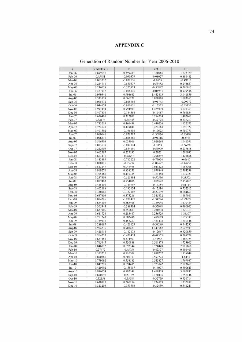
74

APPENDIX C

Generation of Random Number for Year 2006-2010 i RAND ( ) z erf -1 ti,j

Jan-06 0.699645 0.399289 0.370085 1.523379 Feb-06 0.45481 -0.090379 -0.08027 0.886483 Mar-06 0.063732 -0.872536 -1.0558 -0.49313 Apr-06 0.224711 -0.550577 -0.53482 0.243657 May-06 0.236038 -0.527923 -0.50847 0.280915 Jun-06 0.471912 -0.056176 -0.04983 0.929536 Jul-06 0.999341 0.998683 1.443813 3.041859

Aug-06 0.533139 0.066278 0.058805 1.083163 Sep-06 0.095672 -0.808656 -0.91763 -0.29772 Oct-06 0.044674 -0.910651 -1.15355 -0.63136 Nov-06 0.997494 0.994989 1.429319 3.021363 Dec-06 0.407816 -0.184368 -0.16487 0.766834 Jan-07 0.656401 0.312802 0.284724 1.402661 Feb-07 0.32176 -0.35648 -0.32724 0.537217 Mar-07 0.733219 0.466438 0.440226 1.622573 Apr-07 0.724521 0.449041 0.421663 1.596322 May-07 0.401592 -0.196816 -0.17623 0.750771 Jun-07 0.010641 -0.978717 -1.36824 -0.93498 Jul-07 0.096817 -0.806366 -0.91316 -0.2914

Aug-07 0.516508 0.033016 0.029268 1.041391 Sep-07 0.053638 -0.892724 -1.1059 -0.56398 Oct-07 0.222905 -0.554191 -0.53909 0.237618 Nov-07 0.612597 0.225195 0.2023 1.286095 Dec-07 0.663435 0.32687 0.298297 1.421856 Jan-08 0.143889 -0.712222 -0.75074 -0.0617 Feb-08 0.070315 -0.85937 -1.02497 -0.44952 Mar-08 0.523247 0.046495 0.041228 1.058306 Apr-08 0.919276 0.838551 0.978848 2.384299 May-08 0.705168 0.410335 0.381358 1.539321 Jun-08 0.237308 -0.525384 -0.50556 0.28503 Jul-08 0.877403 0.754806 0.819547 2.159015

Aug-08 0.425101 -0.149797 -0.13354 0.81114 Sep-08 0.402188 -0.195624 -0.17514 0.752312 Oct-08 0.338947 -0.322107 -0.29369 0.584661 Nov-08 0.687608 0.375216 0.345832 1.489081 Dec-08 0.014286 -0.971427 -1.34224 -0.89822 Jan-09 0.684203 0.368406 0.339046 1.479484 Feb-09 0.305343 -0.389314 -0.35998 0.490905 Mar-09 0.627906 0.255813 0.230738 1.326313 Apr-09 0.641724 0.283447 0.256729 1.36307 May-09 0.751243 0.502486 0.479699 1.678397 Jun-09 0.729118 0.458237 0.431438 1.610146 Jul-09 0.289185 -0.421629 -0.39299 0.444235

Aug-09 0.954236 0.908473 1.147587 2.622933 Sep-09 0.428914 -0.142173 -0.12667 0.820859 Oct-09 0.264273 -0.471453 -0.44563 0.369778 Nov-09 0.687481 0.374963 0.34558 1.488724 Dec-09 0.765445 0.530889 0.511878 1.723905 Jan-10 0.846072 0.692144 0.720449 2.018868 Feb-10 0.27472 -0.45056 -0.42327 0.401403 Mar-10 0.555255 0.110509 0.098252 1.138949 Apr-10 0.800866 0.601733 0.597223 1.8446 May-10 0.779092 0.558183 0.543827 1.769087 Jun-10 0.847218 0.694435 0.723842 2.023667 Jul-10 0.420992 -0.158017 -0.14097 0.800643

Aug-10 0.996074 0.992148 1.418338 3.005833 Sep-10 0.600695 0.20139 0.180416 1.255146 Oct-10 0.32158 -0.35684 -0.32759 0.536714 Nov-10 0.630127 0.260254 0.234893 1.332189 Dec-10 0.323203 -0.353593 -0.32439 0.541241

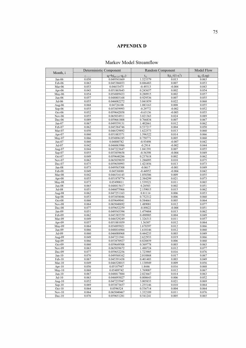
75

APPENDIX D

Markov Model Streamflow

Month, i Deterministic Component Random Component Model Flow qi-1,j-1 qj+bj(qi-1,j-1-qj-1) ti,j Sjti,j√(1-rj

2) qi,j (Log) Jan-06 0.050 0.049541669 1.523379 0.013 0.063 Feb-06 0.063 0.045386033 0.886483 0.007 0.053 Mar-06 0.053 0.04653475 -0.49313 -0.004 0.043 Apr-06 0.043 0.051865643 0.243657 0.002 0.054 May-06 0.054 0.054889433 0.280915 0.002 0.057 Jun-06 0.057 0.048803168 0.929536 0.007 0.055 Jul-06 0.055 0.046082272 3.041859 0.022 0.068

Aug-06 0.068 0.04726108 1.083163 0.008 0.055 Sep-06 0.055 0.053859993 -0.29772 -0.002 0.052 Oct-06 0.052 0.059642058 -0.63136 -0.005 0.055 Nov-06 0.055 0.065034911 3.021363 0.024 0.089 Dec-06 0.089 0.059661808 0.766834 0.007 0.067 Jan-07 0.067 0.049559131 1.402661 0.012 0.062 Feb-07 0.062 0.045384746 0.537217 0.004 0.050 Mar-07 0.050 0.046529892 1.622573 0.013 0.060 Apr-07 0.060 0.051883571 1.596322 0.014 0.066 May-07 0.066 0.054896185 0.750771 0.005 0.060 Jun-07 0.060 0.04880782 -0.93498 -0.007 0.042 Jul-07 0.042 0.046063986 -0.2914 -0.002 0.044

Aug-07 0.044 0.047223647 1.041391 0.007 0.055 Sep-07 0.055 0.053859658 -0.56398 -0.004 0.049 Oct-07 0.049 0.059640286 0.237618 0.002 0.062 Nov-07 0.062 0.065039039 1.286095 0.010 0.075 Dec-07 0.075 0.059650993 1.421856 0.013 0.073 Jan-08 0.073 0.049565308 -0.0617 -0.001 0.049 Feb-08 0.049 0.04536888 -0.44952 -0.004 0.042 Mar-08 0.042 0.046516145 1.058306 0.009 0.055 Apr-08 0.055 0.051878774 2.384299 0.021 0.073 May-08 0.073 0.05490011 1.539321 0.011 0.065 Jun-08 0.065 0.048815617 0.28503 0.002 0.051 Jul-08 0.051 0.046075966 2.159015 0.015 0.062

Aug-08 0.062 0.047251163 0.81114 0.006 0.053 Sep-08 0.053 0.053858046 0.752312 0.006 0.060 Oct-08 0.060 0.059649041 0.584661 0.005 0.064 Nov-08 0.064 0.065040692 1.489081 0.012 0.077 Dec-08 0.077 0.059652259 -0.89822 -0.008 0.051 Jan-09 0.051 0.049543394 1.479484 0.013 0.062 Feb-09 0.062 0.045385559 0.490905 0.004 0.049 Mar-09 0.049 0.046529249 1.326313 0.011 0.057 Apr-09 0.057 0.051881059 1.36307 0.012 0.064 May-09 0.064 0.054895021 1.678397 0.012 0.066 Jun-09 0.066 0.048816984 1.610146 0.012 0.060 Jul-09 0.060 0.046088968 0.444235 0.003 0.049

Aug-09 0.049 0.047231941 2.622933 0.019 0.066 Sep-09 0.066 0.053870927 0.820859 0.006 0.060 Oct-09 0.060 0.059649508 0.369778 0.003 0.063 Nov-09 0.063 0.065039672 1.488724 0.012 0.077 Dec-09 0.077 0.059652256 1.723905 0.016 0.076 Jan-10 0.076 0.049568162 2.018868 0.017 0.067 Feb-10 0.067 0.045391438 0.401403 0.003 0.049 Mar-10 0.049 0.046528015 1.138949 0.009 0.056 Apr-10 0.056 0.05187947 1.8446 0.016 0.068 May-10 0.068 0.05489742 1.769087 0.012 0.067 Jun-10 0.067 0.048817884 2.023667 0.014 0.063 Jul-10 0.063 0.046093027 0.800643 0.006 0.052

Aug-10 0.052 0.047235947 3.005833 0.021 0.069 Sep-10 0.069 0.053873657 1.255146 0.010 0.064 Oct-10 0.064 0.0596524 0.536714 0.004 0.064 Nov-10 0.064 0.065040467 1.332189 0.011 0.076 Dec-10 0.076 0.059651281 0.541241 0.005 0.065

76

APPENDIX E

Performance Evaluation Procedure of Markov Model

i Actual Flow (m3/s)

Model Flow (m3/s)

MAPE RMSE Chi-square Test

Jan-06 13.08 13.533 3.462 0.205001 0.015148 Feb-06 8.12 9.077 11.786 0.915831 0.100896 Mar-06 6.11 5.641 7.681 0.220272 0.039051 Apr-06 29.72 9.604 67.685 404.6583 42.13488 May-06 29.22 10.807 63.015 339.0362 31.37171 Jun-06 17.82 10.210 42.706 57.91601 5.672621 Jul-06 7.94 16.422 106.822 71.93914 4.380738

Aug-06 9.95 10.014 0.644 0.00411 0.00041 Sep-06 28.05 8.642 69.192 376.688 43.59034 Oct-06 17.63 9.821 44.298 61.00476 6.211446 Nov-06 17.72 32.326 82.432 213.3443 6.599874 Dec-06 11.23 15.849 41.109 21.31845 1.345112 Jan-07 9.05 13.020 43.872 15.7641 1.210723 Feb-07 6.80 7.992 17.535 1.421735 0.177887 Mar-07 7.62 12.065 58.336 19.76006 1.637769 Apr-07 13.46 15.262 13.384 3.245474 0.212657 May-07 12.05 12.299 2.069 0.06214 0.005052 Jun-07 11.38 5.514 51.550 34.41474 6.241801 Jul-07 13.06 6.059 53.607 49.01556 8.089859

Aug-07 8.95 9.874 10.339 0.855987 0.086689 Sep-07 9.36 7.877 15.846 2.199906 0.27929 Oct-07 14.33 13.038 9.013 1.668293 0.127953 Nov-07 14.26 21.161 48.391 47.61862 2.250341 Dec-07 8.24 19.599 137.858 129.0379 6.58374 Jan-08 11.29 7.719 31.625 12.74858 1.651481 Feb-08 6.76 5.384 20.351 1.89258 0.3515 Mar-08 9.58 10.032 4.721 0.20453 0.020387 Apr-08 12.86 19.404 50.886 42.82308 2.206928 May-08 9.73 15.098 55.171 28.81687 1.908638 Jun-08 12.28 8.379 31.768 15.21902 1.816363 Jul-08 10.89 13.007 19.439 4.481376 0.344538

Aug-08 7.83 9.219 17.734 1.928084 0.209153 Sep-08 9.85 12.127 23.119 5.185165 0.427585 Oct-08 13.14 14.502 10.398 1.865887 0.12866 Nov-08 16.74 22.302 33.224 30.93221 1.386991 Dec-08 10.96 8.531 22.161 5.899487 0.691526 Jan-09 9.73 13.343 37.128 13.05078 0.97813 Feb-09 9.67 7.856 18.764 3.292187 0.41909 Mar-09 15.10 10.970 27.352 17.05788 1.554974 Apr-09 13.72 14.160 3.205 0.193326 0.013653 May-09 8.75 15.629 78.619 47.32323 3.027875 Jun-09 7.31 12.423 69.942 26.14056 2.104243 Jul-09 8.05 7.800 3.111 0.062732 0.008043

Aug-09 9.03 15.337 69.845 39.77884 2.593644 Sep-09 10.08 12.388 22.897 5.327024 0.430014 Oct-09 7.99 13.587 70.046 31.32252 2.305389

77

Nov-09 12.73 22.299 75.168 91.56381 4.106203 Dec-09 6.88 21.522 212.820 214.3895 9.961389 Jan-10 6.83 15.834 131.827 81.06853 5.119965 Feb-10 4.86 7.597 56.317 7.491085 0.98606 Mar-10 4.36 10.312 136.513 35.42605 3.435427 Apr-10 7.18 16.493 129.701 86.72375 5.258356 May-10 6.17 15.985 159.084 96.34386 6.026957 Jun-10 7.51 13.908 85.191 40.93266 2.943131 Jul-10 7.45 8.744 17.405 1.680274 0.192169

Aug-10 8.04 16.912 110.346 78.70912 4.65409 Sep-10 7.16 14.091 96.798 48.03522 3.408991 Oct-10 6.30 14.296 126.927 63.94217 4.472611 Nov-10 9.56 21.417 124.026 140.5846 6.564209 Dec-10 11.01 14.672 33.261 13.41047 0.914016

53.659 7.29 250.9884

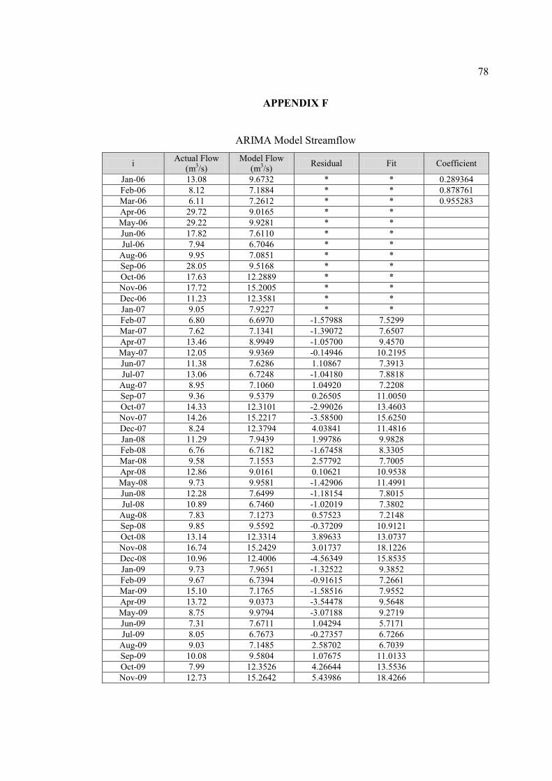
78

APPENDIX F

ARIMA Model Streamflow

i Actual Flow (m3/s)

Model Flow (m3/s) Residual Fit Coefficient

Jan-06 13.08 9.6732 * * 0.289364 Feb-06 8.12 7.1884 * * 0.878761 Mar-06 6.11 7.2612 * * 0.955283 Apr-06 29.72 9.0165 * * May-06 29.22 9.9281 * * Jun-06 17.82 7.6110 * * Jul-06 7.94 6.7046 * *

Aug-06 9.95 7.0851 * * Sep-06 28.05 9.5168 * * Oct-06 17.63 12.2889 * * Nov-06 17.72 15.2005 * * Dec-06 11.23 12.3581 * * Jan-07 9.05 7.9227 * * Feb-07 6.80 6.6970 -1.57988 7.5299 Mar-07 7.62 7.1341 -1.39072 7.6507 Apr-07 13.46 8.9949 -1.05700 9.4570 May-07 12.05 9.9369 -0.14946 10.2195 Jun-07 11.38 7.6286 1.10867 7.3913 Jul-07 13.06 6.7248 -1.04180 7.8818

Aug-07 8.95 7.1060 1.04920 7.2208 Sep-07 9.36 9.5379 0.26505 11.0050 Oct-07 14.33 12.3101 -2.99026 13.4603 Nov-07 14.26 15.2217 -3.58500 15.6250 Dec-07 8.24 12.3794 4.03841 11.4816 Jan-08 11.29 7.9439 1.99786 9.9828 Feb-08 6.76 6.7182 -1.67458 8.3305 Mar-08 9.58 7.1553 2.57792 7.7005 Apr-08 12.86 9.0161 0.10621 10.9538 May-08 9.73 9.9581 -1.42906 11.4991 Jun-08 12.28 7.6499 -1.18154 7.8015 Jul-08 10.89 6.7460 -1.02019 7.3802

Aug-08 7.83 7.1273 0.57523 7.2148 Sep-08 9.85 9.5592 -0.37209 10.9121 Oct-08 13.14 12.3314 3.89633 13.0737 Nov-08 16.74 15.2429 3.01737 18.1226 Dec-08 10.96 12.4006 -4.56349 15.8535 Jan-09 9.73 7.9651 -1.32522 9.3852 Feb-09 9.67 6.7394 -0.91615 7.2661 Mar-09 15.10 7.1765 -1.58516 7.9552 Apr-09 13.72 9.0373 -3.54478 9.5648 May-09 8.75 9.9794 -3.07188 9.2719 Jun-09 7.31 7.6711 1.04294 5.7171 Jul-09 8.05 6.7673 -0.27357 6.7266

Aug-09 9.03 7.1485 2.58702 6.7039 Sep-09 10.08 9.5804 1.07675 11.0133 Oct-09 7.99 12.3526 4.26644 13.5536 Nov-09 12.73 15.2642 5.43986 18.4266

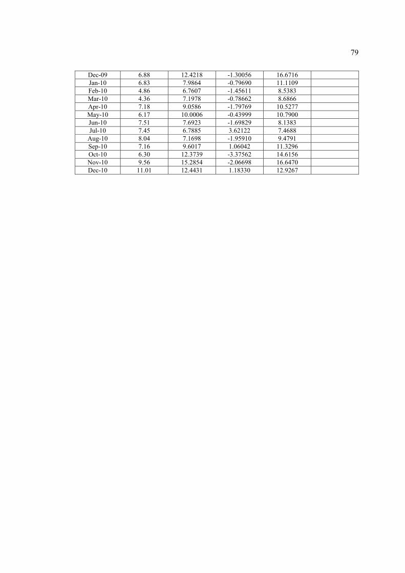
79

Dec-09 6.88 12.4218 -1.30056 16.6716 Jan-10 6.83 7.9864 -0.79690 11.1109 Feb-10 4.86 6.7607 -1.45611 8.5383 Mar-10 4.36 7.1978 -0.78662 8.6866 Apr-10 7.18 9.0586 -1.79769 10.5277 May-10 6.17 10.0006 -0.43999 10.7900 Jun-10 7.51 7.6923 -1.69829 8.1383 Jul-10 7.45 6.7885 3.62122 7.4688

Aug-10 8.04 7.1698 -1.95910 9.4791 Sep-10 7.16 9.6017 1.06042 11.3296 Oct-10 6.30 12.3739 -3.37562 14.6156 Nov-10 9.56 15.2854 -2.06698 16.6470 Dec-10 11.01 12.4431 1.18330 12.9267

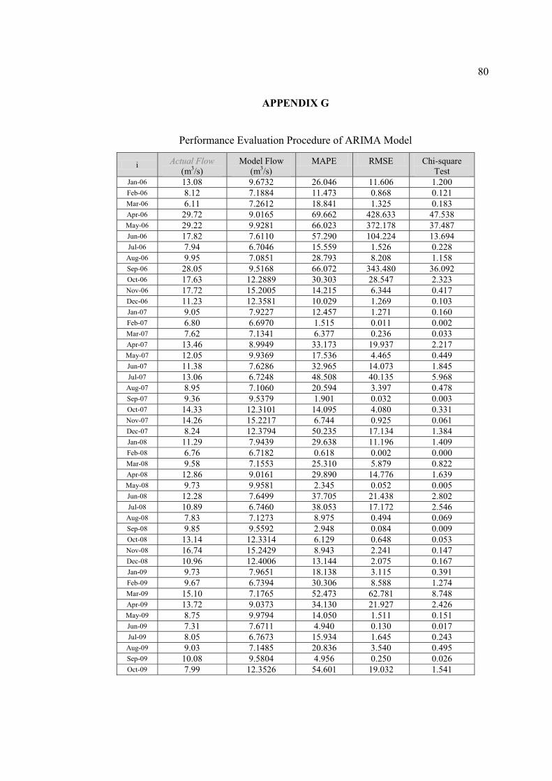
80

APPENDIX G

Performance Evaluation Procedure of ARIMA Model

i Actual Flow (m3/s)

Model Flow (m3/s)

MAPE RMSE Chi-square Test

Jan-06 13.08 9.6732 26.046 11.606 1.200 Feb-06 8.12 7.1884 11.473 0.868 0.121 Mar-06 6.11 7.2612 18.841 1.325 0.183 Apr-06 29.72 9.0165 69.662 428.633 47.538 May-06 29.22 9.9281 66.023 372.178 37.487 Jun-06 17.82 7.6110 57.290 104.224 13.694 Jul-06 7.94 6.7046 15.559 1.526 0.228

Aug-06 9.95 7.0851 28.793 8.208 1.158 Sep-06 28.05 9.5168 66.072 343.480 36.092 Oct-06 17.63 12.2889 30.303 28.547 2.323 Nov-06 17.72 15.2005 14.215 6.344 0.417 Dec-06 11.23 12.3581 10.029 1.269 0.103 Jan-07 9.05 7.9227 12.457 1.271 0.160 Feb-07 6.80 6.6970 1.515 0.011 0.002 Mar-07 7.62 7.1341 6.377 0.236 0.033 Apr-07 13.46 8.9949 33.173 19.937 2.217 May-07 12.05 9.9369 17.536 4.465 0.449 Jun-07 11.38 7.6286 32.965 14.073 1.845 Jul-07 13.06 6.7248 48.508 40.135 5.968

Aug-07 8.95 7.1060 20.594 3.397 0.478 Sep-07 9.36 9.5379 1.901 0.032 0.003 Oct-07 14.33 12.3101 14.095 4.080 0.331 Nov-07 14.26 15.2217 6.744 0.925 0.061 Dec-07 8.24 12.3794 50.235 17.134 1.384 Jan-08 11.29 7.9439 29.638 11.196 1.409 Feb-08 6.76 6.7182 0.618 0.002 0.000 Mar-08 9.58 7.1553 25.310 5.879 0.822 Apr-08 12.86 9.0161 29.890 14.776 1.639 May-08 9.73 9.9581 2.345 0.052 0.005 Jun-08 12.28 7.6499 37.705 21.438 2.802 Jul-08 10.89 6.7460 38.053 17.172 2.546

Aug-08 7.83 7.1273 8.975 0.494 0.069 Sep-08 9.85 9.5592 2.948 0.084 0.009 Oct-08 13.14 12.3314 6.129 0.648 0.053 Nov-08 16.74 15.2429 8.943 2.241 0.147 Dec-08 10.96 12.4006 13.144 2.075 0.167 Jan-09 9.73 7.9651 18.138 3.115 0.391 Feb-09 9.67 6.7394 30.306 8.588 1.274 Mar-09 15.10 7.1765 52.473 62.781 8.748 Apr-09 13.72 9.0373 34.130 21.927 2.426 May-09 8.75 9.9794 14.050 1.511 0.151 Jun-09 7.31 7.6711 4.940 0.130 0.017 Jul-09 8.05 6.7673 15.934 1.645 0.243

Aug-09 9.03 7.1485 20.836 3.540 0.495 Sep-09 10.08 9.5804 4.956 0.250 0.026 Oct-09 7.99 12.3526 54.601 19.032 1.541

81

Nov-09 12.73 15.2642 19.907 6.422 0.421 Dec-09 6.88 12.4218 80.550 30.712 2.472 Jan-10 6.83 7.9864 16.931 1.337 0.167 Feb-10 4.86 6.7607 39.109 3.613 0.534 Mar-10 4.36 7.1978 65.087 8.053 1.119 Apr-10 7.18 9.0586 26.164 3.529 0.390 May-10 6.17 10.0006 62.085 14.674 1.467 Jun-10 7.51 7.6923 2.428 0.033 0.004 Jul-10 7.45 6.7885 8.848 0.434 0.064

Aug-10 8.04 7.1698 10.824 0.757 0.106 Sep-10 7.16 9.6017 34.102 5.962 0.621 Oct-10 6.30 12.3739 96.411 36.892 2.981 Nov-10 9.56 15.2854 59.889 32.780 2.145 Dec-10 11.01 12.4431 13.016 2.054 0.165

27.497 5.416 191.114