arX

iv:a

stro

-ph/

0611

070v

2 1

9 F

eb 2

007

Astronomy & Astrophysicsmanuscript no. 6228 c© ESO 2018October 30, 2018

High-resolution spectroscopy ofRGB stars in the Sagittarius Streams ⋆

I. Radial velocities and chemical abundances

L. Monaco1, M. Bellazzini2, P. Bonifacio3,4,5, A. Buzzoni2,F.R. Ferraro6, G. Marconi1, L. Sbordone5,7, and S. Zaggia8

1 European Southern Observatory, Casilla 19001, Santiago, Chile2 Istituto Nazionale di Astrofisica – Osservatorio Astronomico di Bologna, Italy I-40127 Bologna, Italy3 CIFIST Marie Curie Excellence Team4 Observatoire de Paris, GEPI , 5, place Jules Janssen, 92195 Meudon, France5 Istituto Nazionale di Astrofisica – Osservatorio Astronomico di Trieste, Via Tiepolo 11, I-34131 Trieste, Italy6 Universita di Bologna – Dipartimento di Astronomia, I-40127 Bologna, Italy7 Istituto Nazionale di Astrofisica – Osservatorio Astronomico di Roma, Via Frascati 33, 00040 Monteporzio Catone, Roma,Italy8 Istituto Nazionale di Astrofisica – Osservatorio Astronomico di Padova, Vicolo dell’Osservatorio 5, 35122 Padova, Italy

Received/ Accepted

ABSTRACT

Context. The Sagittarius (Sgr) dwarf spheroidal galaxy is currentlybeing disrupted under the strain of the Milky Way. A reliablereconstructionof Sgr star formation history can only be obtained by combining core and stream information.Aims. We present radial velocities for 67 stars belonging to the Sgr Stream. For 12 stars in the sample we also present iron (Fe) andα-element(Mg, Ca) abundances.Methods. Spectra were secured using different high resolution facilities: UVES@VLT, HARPS@3.6m, and SARG@TNG. Radial velocitiesare obtained through cross correlation with a template spectra. Concerning chemical analysis, for the various elements, selected line equivalentwidths were measured and abundances computed using the WIDTH code and ATLAS model atmospheres.Results. The velocity dispersion of the trailing tail is found to beσ=8.3±0.9 km s−1, i.e., significantly lower than in the core of the Sgr galaxyand marginally lower than previous estimates in the same portion of the stream. Stream stars follow the same trend as Sgr main body stars inthe [α/Fe] vs [Fe/H] plane. However, stars are, on average, more metal poor in the stream than in the main body. This effect is slightly strongerin stars belonging to more ancient wraps of the stream, according to currently accepted models of Sgr disruption.

Key words. Stars: abundances – Stars: atmospheres – Galaxies: abundances – Galaxies: evolution – Galaxies: dwarf – Galaxies: individual:Sgr dSph

Send offprint requests to: L. Monaco⋆ Based on observations taken at ESO VLT Kueyen telescope

(Cerro Paranal, Chile, program: 075.B-0127(A)) and 3.6m telescope(La Silla, Chile). Also based on spectroscopic observations takenat the Telescopio Nazionale Galileo, operated by the FundacionG. Galilei of INAF at the Spanish Observatorio del Roque de losMuchachos of the IAC (La Palma, Spain).Correspondence to: lmonaco@eso.org

1. Introduction

Dwarfs are the most common type of galaxies in the universe.Several dwarf satellites are usually associated with giantgalax-ies and, in the commonly accepted scenario (White & Rees1978), giant galaxies actually emerge out of the hierarchicalassembly of dwarfs. In this respect, dwarf galaxies are consid-ered to be the building blocks of the universe.

The Sagittarius dwarf spheroidal galaxy(Ibata, Gilmore, & Irwin 1994, Sgr dSph) is currentlydisrupting into the Milky Way (MW) and its discovery

2 Monaco et al.: RGB stars in the Sgr dSph Streams

Table 1. Basic parameters of the program stars. Measured radial velocities and spectra signal-to-noise ratios are also reported.Beside the 2MASS name we give our own identifier to the star, which is used consequently in the other tables and throughout thepaper.

SARG sample

2MASS ID Star α (J2000.0) δ (J2000.0) l b Λ⊙ K0 (J − K)0 E(B-V) d⊙(kpc) S/N vhelio(km/s) vgsr(km/s)(@650nm)

2MASS J00170214+0104165 1 00 17 02.1 +01 04 16 105.2 -60.6 82.18 10.88 0.95 0.03 15.07 19 -227.91±0.48 -125.292MASS J01225543+0451341 19 01 22 55.4 +04 51 34 137.5 -57.1 98.69 10.89 0.97 0.03 16.39 29 -207.07±0.45 -131.442MASS J01295300+0055392 23 01 29 53.0 +00 55 39 142.7 -60.5 98.08 11.21 0.94 0.02 16.42 29 -163.52±0.25 -103.862MASS J01305453+0351575 25 01 30 54.5 +03 51 57 141.5 -57.6 99.86 11.19 0.96 0.02 18.22 27 -188.82±0.30 -121.112MASS J01492111+0231536 39 01 49 21.1 +02 31 53 150.4 -57.2 103.1 10.77 0.99 0.02 16.43 32 -188.31±0.51 -136.392MASS J01520195+0020525 42 01 52 01.9 +00 20 52 153.3 -58.9 102.5 10.73 0.96 0.03 14.56 33 -160.10±0.33 -116.452MASS J02224517+0039362 77 02 22 45.1 +00 39 36 165.0 -54.6 109.2 10.64 0.97 0.03 14.20 37 -45.94±0.34 -21.79

2MASS J08491184+4819380 232 08 49 11.8 +48 19 38 171.2 39.2 202.9 11.10 0.97 0.03 17.69 18 -27.77±0.20 -2.852MASS J09193349+4350034 242 09 19 33.5 +43 50 03 176.9 44.6 208.9 10.31 0.95 0.02 11.48 28 -8.24±0.19 -0.902MASS J10055844+3132597 260 10 05 58.4 +31 33 00 195.8 53.9 220.5 10.48 0.97 0.02 13.53 8 107.71±0.33 71.122MASS J10413374+4033099 278 10 41 33.8 +40 33 10 177.9 60.1 224.8 11.35 0.93 0.02 17.15 17 30.69±0.37 36.582MASS J10472976+2339508 281 10 47 29.8 +23 39 51 213.0 61.9 231.6 10.13 0.94 0.03 10.07 25 56.53±0.41 -0.492MASS J10504744+2748542 283 10 50 47.5 +27 48 54 204.4 63.3 230.9 10.62 0.95 0.02 13.09 15 -25.32±0.48 -65.83

HARPS sample

2MASS J13091343+1215502 465 13 09 13.4 +12 15 50 319.5 74.6 266.8 10.35 0.99 0.02 13.51 2 -30.57±0.011 -62.142MASS J14340509+0936258 677 14 34 05.1 +09 36 26 1.9 60.1 286.0 9.60 0.99 0.03 9.64 2 -73.55±0.011 -59.132MASS J09364419+0704484 452892 09 36 44.2 +07 04 48 227.2 39.7 219.5 9.94 0.94 0.04 10.18 12 118.53±0.008 -12.522MASS J09453656+0937568 459992 09 45 36.6 +09 37 57 225.6 42.9 221.2 9.91 0.99 0.02 11.47 12 336.10±0.008 214.812MASS J09564707+0645292 452060 09 56 47.1 +06 45 29 230.9 43.9 224.8 9.82 0.95 0.02 9.62 12 100.57±0.008 -28.532MASS J11345053-0700511 421173 11 34 50.5 -07 00 51 271.7 51.1 255.3 9.81 0.97 0.04 10.84 11 69.26±0.008 -70.602MASS J11554802-0339068 427535 11 55 48.0 -03 39 07 277.2 56.4 258.6 10.01 0.99 0.02 12.42 7 -57.53±0.009 -178.382MASS J14112205-0610129 423286 14 11 22.1 -06 10 13 336.0 51.5 289.7 9.51 1.05 0.03 12.55 12 41.10±0.008 -7.04

UVES sample

2MASS J00035283-1940468 1005 00 03 52.8 -19 40 47 64.8 -76.8 69.5 10.97 1.03 0.02 19.1 31 -56.92± 0.13 -14.932MASS J00131891-2301528 1006 00 13 18.9 -23 01 53 56.2 -80.4 70.1 10.59 1.00 0.02 14.5 42 -41.90± 0.05 -15.822MASS J00135624-1721554 1007 00 13 56.2 -17 21 55 79.4 -76.9 72.7 11.52 0.99 0.03 21.4 53 -90.51± 0.16 -45.262MASS J00223563-0512079 1008 00 22 35.6 -05 12 08 104.3 -67.080.0 9.81 1.08 0.03 13.9 38 -116.25± 0.31 -35.722MASS J00264668-1526427 1009 00 26 46.7 -15 26 43 95.6 -77.0 76.3 10.82 0.95 0.03 13.2 49 -70.01± 0.07 -25.092MASS J00321654-1851113 1010 00 32 16.5 -18 51 11 93.9 -80.6 75.9 11.57 1.02 0.02 24.5 29 -71.25± 0.10 -40.452MASS J00390964-1322429 1011 00 39 09.6 -13 22 43 110.5 -76.079.9 10.50 1.12 0.02 21.9 18 -95.24± 0.22 -50.222MASS J00464414-0659259 1013 00 46 44.1 -06 59 26 119.5 -69.884.5 11.84 0.95 0.06 21.0 49 -122.67± 0.51 -61.052MASS J00480460-1131551 1014 00 48 04.6 -11 31 55 119.9 -74.482.7 10.61 1.05 0.03 17.3 47 -100.88± 0.46 -54.742MASS J00522982-1518360 1015 00 52 29.8 -15 18 36 124.2 -78.281.9 11.16 1.08 0.02 25.3 21 -87.05± 0.67 -55.702MASS J00532013-0529477 1016 00 53 20.1 -05 29 48 124.2 -68.486.7 10.46 1.01 0.04 14.0 55 -148.81± 0.45 -86.552MASS J00542073-0449174 1017 00 54 20.7 -04 49 17 124.8 -67.787.3 10.51 1.01 0.05 14.3 47 -139.50± 0.42 -75.632MASS J00563325-2154386 1018 00 56 33.3 -21 54 39 135.8 -84.779.5 10.74 1.06 0.02 19.2 29 -56.01± 0.09 -48.642MASS J01011934-1536343 1019 01 01 19.3 -15 36 34 134.7 -78.383.6 11.20 1.01 0.02 19.6 52 -86.01± 0.55 -60.712MASS J01015376-1015085 1020 01 01 53.8 -10 15 08 131.7 -72.986.3 11.31 1.01 0.03 21.0 63 -119.20± 0.53 -76.722MASS J01091912-1508157 1022 01 09 19.1 -15 08 16 143.0 -77.385.5 9.27 1.14 0.03 13.6 18 -102.48± 0.43 -80.192MASS J01212317-1036096 1025 01 21 23.2 -10 36 10 147.5 -72.090.3 10.06 1.08 0.03 15.5 38 -139.46± 0.16 -109.942MASS J01282756-0505173 1028 01 28 27.6 -05 05 17 146.4 -66.394.6 11.33 0.96 0.04 17.1 71 -123.43± 0.52 -81.252MASS J01512105-0727451 1034 01 51 21.1 -07 27 45 161.5 -65.798.3 11.69 1.01 0.02 24.4 52 -129.68± 0.37 -109.282MASS J01574156-1709471 1035 01 57 41.6 -17 09 47 183.3 -71.794.6 10.65 1.05 0.02 17.5 28 -91.39± 0.11 -105.052MASS J01593606-0801131 1036 01 59 36.1 -08 01 13 166.3 -65.099.8 10.66 1.05 0.02 18.0 32 -109.87± 0.27 -96.692MASS J21153360-3530060 1065 21 15 33.6 -35 30 06 8.5 -43.7 29.5 11.73 1.03 0.07 26.7 47 90.93± 0.22 117.322MASS J21174714-2432331 1066 21 17 47.1 -24 32 33 23.4 -42.2 31.5 11.92 1.01 0.05 27.4 44 30.30± 0.03 99.972MASS J21250780-2747090 1067 21 25 07.8 -27 47 09 19.6 -44.6 32.6 10.65 1.00 0.10 14.5 38 52.99± 0.21 109.522MASS J21314538-3513510 1068 21 31 45.4 -35 13 51 9.3 -47.0 32.8 11.65 1.01 0.07 24.0 48 81.00± 0.14 107.512MASS J21581991-3406074 1071 21 58 19.9 -34 06 07 11.4 -52.4 38.4 10.74 1.07 0.02 20.0 61 49.80± 0.05 77.622MASS J22083965-2812124 1072 22 08 39.7 -28 12 12 21.5 -54.1 42.0 10.92 1.04 0.02 19.1 35 34.80± 0.28 83.892MASS J22142679-2306184 1073 22 14 26.8 -23 06 18 30.5 -54.4 44.5 10.24 1.10 0.03 17.8 23 -11.35± 0.40 56.012MASS J22264953-3918313 1075 22 26 49.5 -39 18 31 1.5 -57.7 42.7 10.86 1.01 0.02 16.5 47 78.46± 0.21 80.602MASS J22373980-2628544 1076 22 37 39.8 -26 28 54 26.4 -60.2 48.6 10.35 1.04 0.02 14.7 49 15.13± 0.22 64.332MASS J22392246-2508120 1077 22 39 22.5 -25 08 12 29.2 -60.4 49.4 9.99 1.10 0.02 15.7 18 -16.66± 0.46 37.042MASS J22442231-3247156 1078 22 44 22.3 -32 47 16 13.5 -62.0 48.1 11.21 1.03 0.01 21.5 27 22.16± 0.11 45.522MASS J22561212-2045555 1080 22 56 12.1 -20 45 56 40.3 -63.0 54.4 11.24 0.99 0.03 18.6 70 -50.66± 0.16 14.342MASS J23194353-1546105 1082 23 19 43.5 -15 46 11 56.3 -65.9 61.4 11.24 1.03 0.03 21.8 63 -78.77± 0.39 -4.312MASS J23212651-2426543 1083 23 21 26.5 -24 26 54 35.4 -69.6 58.6 10.50 1.14 0.02 24.0 14 -19.21± 0.16 23.632MASS J23241474-2750339 1084 23 24 14.7 -27 50 34 25.8 -70.7 57.9 11.46 1.04 0.02 24.9 34 -1.30± 0.39 28.152MASS J23262366-2500371 1085 23 26 23.7 -25 00 37 34.5 -70.8 59.4 10.78 1.00 0.02 15.7 52 -20.79± 0.14 18.252MASS J23293008-2458096 1086 23 29 30.1 -24 58 10 35.0 -71.5 60.1 10.46 1.10 0.02 20.1 15 -33.59± 0.32 4.342MASS J23295478-2051034 1087 23 29 54.8 -20 51 03 47.2 -70.4 61.8 10.59 1.00 0.04 14.4 53 -42.89± 0.10 9.672MASS J23303457-1607474 1088 23 30 34.6 -16 07 47 59.2 -68.3 63.7 11.30 0.98 0.03 17.9 71 -64.25± 0.25 4.632MASS J23430789-2358264 1089 23 43 07.9 -23 58 27 40.7 -74.3 63.4 11.35 0.97 0.02 17.8 39 -29.11± 0.08 6.932MASS J23454168-2644555 1090 23 45 41.7 -26 44 56 30.7 -75.4 62.8 10.38 1.02 0.02 14.0 48 -14.45± 0.15 10.582MASS J23503612-2002156 1091 23 50 36.1 -20 02 16 56.7 -74.4 66.5 10.58 1.07 0.02 18.4 33 -55.91± 0.30 -9.182MASS J23531941-2050407 1092 23 53 19.4 -20 50 41 55.2 -75.3 66.8 11.61 0.97 0.02 20.1 55 -52.74± 0.08 -9.872MASS J23563742-2347116 1093 23 56 37.4 -23 47 12 45.0 -77.2 66.3 11.46 0.99 0.02 20.8 59 -41.64± 0.20 -10.712MASS J23565416-1906094 1094 23 56 54.2 -19 06 09 62.7 -75.1 68.3 11.64 1.03 0.02 25.6 49 -61.81± 0.19 -14.50

Monaco et al.: RGB stars in the Sgr dSph Streams 3

historically represented one of the first clear confirmationson a local framework of the hierarchical merging paradigm.Nevertheless, the chemical analysis of stars in the MWsatellites and in Sgr itself seems to seriously challenge thisevolutionary scheme (see Venn et al. 2004 for a review). Infact, it turned out that red giant stars in local dwarfs havechemical patterns, in particular in the [α/Fe] abundance ratios,that are not compatible with those of the galactic halo (but seeRobertson et al. 2005, for a possible solution to this problem).However, the idea that dwarfs may have contributed the halowith stars even significantly different from their present stellarpopulation is now under investigation (Munoz et al. 2006;Chou et al. 2006).

Tagging accreted components and analyzing their chem-ical composition is very important for our comprehensionof the Milky Way formation. Some streams were identifiedin the galaxy without any association with a core remnant.Therefore, they could represent the residuals of ancient ac-cretions (Duffau et al. 2006; Belokurov et al. 2006a), and theirchemical signature might be very informative as well.

In this framework, Sgr plays a special role. It presents avery significant core remnant (30◦ tidal radius), and its gianttidal streams (henceforth, the Stream, for brevity), now iden-tified all over the sky (Majewski et al. 2003, hereafter M03),indicate that the disruption process is still ongoing. Hence, Sgris a MW satellite for which a complete reconstruction of thestar formation history is possible, combining core and streaminformation. As such, it will be possible to understand if Sgr isactually a building block of the galactic halo or not. Deep colormagnitude diagrams (e.g., Marconi et al. 1998; Bellazzini et al.1999; Layden & Sarajedini 2000; Monaco et al. 2002;Bellazzini et al. 2006a) and abundances derived from highresolution spectra (Bonifacio et al. 2000; McWilliam et al.2003; Bonifacio et al. 2004; McWilliam & Smecker-Hane2005; Monaco et al. 2005; Sbordone et al. 2006) provided afresh wealth of information about the star formation history(SFH) of the stellar populations present in the Sgr core overtheyears. Information about the Stream is now also accumulating(M03, Majewski et al. 2004; Law et al. 2005; Belokurov et al.2006b; Chou et al. 2006; Bellazzini et al. 2006b).

This is the first paper of a series devoted to the study ofthe Sgr Stream. Here, we present radial velocities for 67 redgiant branch (RGB) stars belonging to the Stream and high res-olution chemical abundances (Fe, Mg, and Ca) for 12 of thesestars. The paper is organized as follows: in§2 we describe thetarget selection procedure. The observational dataset andtheapplied data reduction procedure are discussed in§3. In §4 wedescribe the procedure for radial velocity measurements anddiscuss the obtained results. In§5 we present a comparisonbetween radial velocity obtained here and in Majewski et al.(2004, hereafter M04) for a sample of stars belonging to the Sgrtrailing tail and common to the two studies. In§6 we presentchemical abundances obtained for 12 stars lying in two differ-

ent spots of the Stream. In§7 we discuss our findings. In§8 webriefly summarize the obtained results.

2. Target selection

Data were obtained using three different high resolution fa-cilities. A sub-sample of the M04 stars was observed withUVES (46 stars). The remaining stars were selected from the2MASS1 catalog employing the M03 procedure, which has al-ready been proven to be a powerful tool to pick-out candidatestream stars (see also M04).

Reddening estimates were obtained through theSchlegel et al. (1998) reddening maps. Distances of thetarget stars were derived through photometric parallax, fol-lowing M03, but adopting (m-M)0= 17.10 as the distancemodulus of the Sgr core (Monaco et al. 2004), instead of16.90. Cartesian coordinates and longitudes in the Sgr orbitalplane were derived following M03 (see M03 for definitionsand details). Coordinates, magnitudes, and derived distances ofthe program stars are listed in Table 1. Parameters for UVESstars are taken directly from Table 3 in M04.

In Fig. 1 we plot the position of the target stars (big solidmarkers) in Cartesian coordinates of the (galactocentric)Sgrorbital plane. Different symbols correspond to stars observedwith different facilities. The Law et al. (2005) model of Sgr de-struction (for a spherical galactic potential) is also plotted forreference.

3. Observations and data reduction

A total of 13 stars were observed between August 30, 2004, andJanuary 24, 2005, using the SARG spectrograph mounted onthe Telescopio Nazionale Galileo (TNG) telescope at La Palma.We used the 1.′′6 slit, which provides a resolution of R=29000.The chosen setup used the yellow cross-disperser, which cov-ers approximately the 462–792 nm spectral range. Data reduc-tion (bias subtraction, division by flat field, lambda calibration,background subtraction, and extraction) was performed withinthe ESO-MIDAS2 echelle context.

During a technical-time slot on the nights of June 3 and4, 2006, we observed 8 supplementary stars with the HARPSfacility mounted at the 3.6m telescope in La Silla. The stan-dard high resolution HARPS mode (R=110000, 380–690 nmspectral range) was employed. Stars were observed for an in-tegration time ranging from 800s (#465) to 1200s (all the oth-ers). Additional HARPS observations were obtained for stars#1006, #1022, and #1083 in July 2006, with 30 min exposures.The June 29, 2006 star #1006 was observed for one hour inte-gration time.

1 See http://www.ipac.caltech.edu/2mass.2 ESO-MIDAS is the acronym for the European Southern

Observatory Munich Image Data Analysis System, devel-oped and maintained by the European Southern Observatory.http://www.eso.org/projects/esomidas/.

4 Monaco et al.: RGB stars in the Sgr dSph Streams

Fig. 1. Program stars positions in the Cartesian galactocen-tric Sgr plane (filled symbols). Different symbols correspondto stars observed with different spectrographs. A model of theSgr disruption (grey dots) is also plotted. The galactic plane(dashed line) and the position of the Sun, of the galactic center,and of the Sgr main body are also marked for reference.

Data were reduced through the online automatic pipelineinstalled on the WHALDRS workstation at the 3.6m controlroom. The final output of the HARPS pipeline is extractedspectra that are completely reduced (bias-subtraction, cosmicrays filtering, flat-field, and wavelength calibration), andthestar radial velocity as measured by a cross correlation func-tion on the bidimensional echelle spectrum with a templateG2 dwarf3 mask. The extreme stability of the HARPS facil-ity secures accurate radial velocity measures even with verylow signal-to-noise spectra. In Fig. 2 we plot the cross correla-tion function obtained for the two lowest S/N spectra obtained.The signal corresponding to the star radial velocity is clearlyevident.

UVES spectra for 46 stars were obtained between June 18and September 16, 2005. Stars were observed with the stan-dard setting DIC 390+580 nm, which covers the spectral range328–456 nm and 480–680 nm, with the Blue and Red arms, re-spectively. We employed a 2×2 CCD binning and a slit width of1.′′2, which provide a resolution of about 35000÷40000. Datawere reduced using the UVES ESO-MIDAS pipeline.

3 To date, the G2 dwarf is the only template available for crosscor-relation using the HARPS pipeline. However, using a not yet releasedM4 mask, we found a∼100 m s−1 radial velocity difference in a testmade on star #459992.

Fig. 2. Cross correlation function (CCF) of the two lowestsignal-to-noise HARPS spectra with the G2 dwarf template.The heliocentric star radial velocity reported in Table 1 isob-tained through a Gaussian fit to the observed peak. Contraryto usual conventions, the star radial velocity is found by theHARPS pipeline as a minimum in the CCF.

4. Radial velocities

Radial velocities (RV) of star in the SARG and UVES samplesare obtained by cross correlation with a synthetic spectrumus-ing thefxcor task inside the IRAF4 suite. The synthetic spec-trum was calculated employing the SYNTHE code (Kurucz1993a; Sbordone, Bonifacio, Castelli, & Kurucz 2004) and aset of atmospheric parameters (temperature; gravity; metallic-ity=3900; 1.0; -0.5) similar to those of all the observed stars(see, e.g., Table 3). Concerning the HARPS spectra, the formalphoton noise induced radial velocity error is in the worst case11 m s−1. A conservative 200 m s−1 uncertainty is assumed. InTable 1 we report the measured radial velocities (heliocentricand in the galactic standard of rest5), as well as the signal-to-noise ratio of the spectra. Radial velocities are obtained witha precision, generally, better than 0.5 km s−1. For the HARPSand UVES spectra, we only present radial velocities, here.

4 IRAF is distributed by the National Optical AstronomyObservatories, which is operated by the association of Universities forResearch in Astronomy, Inc., under contract with the National ScienceFoundation.

5 A local standard of rest rotation velocity of 220 kms−1and a pe-culiar motion of (u,v,w)=(-9,12,7) kms−1are adopted for the Sun, forconsistency with M04.

Monaco et al.: RGB stars in the Sgr dSph Streams 5

Fig. 3. Galactic standard of rest radial velocities of the programstars (filled symbols) as a function of the longitude of the Sgrorbital plane. Different symbols correspond to stars observedwith different spectrographs (circles, squares, and triangles forSARG, HARPS, and UVES data, respectively). Stars studiedby M04 (empty squares) and by Dohm-Palmer et al. (2001)(open triangles) are also plotted together with a model of theSgr disruption (grey dots).

In Fig. 3 we plot the program stars RVs (in the galacticstandard of rest, vgsr) as a function of the Sgr longitude scale(Λ⊙) along the orbital plane. We also plot M04 (for distanceslarger than 13 kpc) and Dohm-Palmer et al. (2001) data super-posed to the Sgr destruction model already used in Fig. 1. Starsin the UVES sample describe a characteristic trend of decreas-ing vgsr with increasingΛ⊙ along the Sgr trailing tail, as al-ready discussed by M04. The same trend is also followed bySARG stars at similar stream positions. Referring to Fig. 1,atpositive galactic latitude (b>0 or YS gr,GC <0) all the SARGand 3 among the HARPS stars lie on a well defined branch ofstream (XS gr,GC <-10 kpc). The large dispersion shown by thisgroup in Fig. 3 (Λ⊙ < 230◦) is predicted to some extent bythe model, and more data are mandatory to constrain the radialvelocity pattern of this part of the stream. The remaining partof the HARPS stars lie in a region where different branches ofthe Sgr Stream overlap (XS gr,GC >-10 kpc in Fig. 1). Their ra-dial velocities nicely fit with the trend predicted by the modelfor the Sgr leading tail and confirmed by Dohm-Palmer et al.(2001) (Fig. 3) and Law et al. (2005) data. However, especiallyfor the three stars at 230◦ < Λ⊙ < 280◦, some ambiguity stillholds.

Fig. 4. Distribution of the difference between RVs measuredhere and in M04. The best-fit Gaussian curve (σ=5.45 km s−1)is also plotted. Long dashed and short dashed lines mark 2σ

and 3σ levels.

5. The UVES sample: comparison with Majewski etal. (2004)

5.1. Sanity check and possible binary stars

UVES stars were selected out of the M04 sample and trace 70degrees of the Sgr trailing tail, in the range 30◦ < Λ⊙ < 100◦.Note thatΛ⊙=0 at the Sgr core. Figure 4 shows the distribu-tion of the differences between the heliocentric radial veloc-ity measured here and in M04 (see Table 1). After removingstar #1006 (which shows a remarkably large velocity differ-ence: -35.4 km s−1), the distribution is well represented by aGaussian distribution centered at -0.44 km s−1 and having aσof 5.45 km s−1. Hence, there is no zero point difference be-tween the two sets of measures and, given the high accuracy ofthe UVES velocities, the dispersion of the distribution nicelyconfirms the 5.3 km s−1 quoted by M04 as random errors.

It is noteworthy that 3 stars lie over the 3σ limit(>16 kms−1of RV variation, Fig. 4). A possible reason for thedetected RV difference is that these stars are in fact binary sys-tems, observed at different orbital phases. Time series of RVmeasures are clearly needed to assess this hypothesis on a firmbasis. Between June and July 2006, additional HARPS datawas obtained for these stars. In Table 2 we report a summary ofthe RVs measured for stars #1006, #1022, and #1083. Supportof the binary hypothesis is provided by this new data to star#1006 and, to some extent, also to #1022, while no significantRV variation between the UVES and HARPS measures was ob-tained for star #1083. In any case, considering the 3 outliers asgenuine binaries, a preliminary lower limit for the Sgr binaryfraction of∼6% is derived.

6 Monaco et al.: RGB stars in the Sgr dSph Streams

Table 2. Heliocentric radial velocity at different dates for thethree suspected binaries. Brackets besides dates acknowledgeUVES (U), HARPS (H), or M04 measures. The last column re-ports the signal-to-noise ratio of the HARPS and UVES spectraor the cross-correlation quality index for M04 data.

v (kms−1)Date 1006 1022 1083 Q

2002-07-15 (M04) -0.1 72002-07-30 (M04) -82.8 52002-07-31 (M04) -6.5 7

S/N2005-07-19 (U) -19.21 142005-07-20 (U) -41.90 422005-09-13 (U) -102.48 182006-06-29 (H) -46.65 102006-07-14 (H) -105.14 92006-07-15 (H) -19.71 82006-07-17 (H) -47.33 132006-07-19 (H) -47.25 -104.64 12, 11

5.2. The velocity dispersion of the Sgr trailing tail

In the upper panels of Fig. 5, we plot the vgsr as a functionof Λ⊙ for stars in the UVES sample. The left panel shows ourmeasures, and the right panel M04 RVs. Continuous lines showa least-squares fit and a polynomial fit (M04) to the trend, inthe former and latter cases, respectively. The fits hold up toΛ⊙ <90◦, where the increase of the velocity dispersion is evi-dent (see M04).

Lower panels show the distribution of differences betweenthe actual RV and the fit. M04 data (right panel) is well fittedby a Gaussian curve having a dispersion of 11.8 kms−1, oncestar #1006 (which lies more than 3σ away from the mean) isremoved. M04 used aσ=11.7 kms−1Gaussian curve to fit theobserved distribution. Hence, the stars we observed are rep-resentative of the more populous M04 sample. Note also thatM04 used 45 stars to evaluate the stream velocity dispersion, anumber not so different from the 40 objects we use here.

The left lower panel shows residuals of our measures withrespect to the fit. The distribution is fitted by a Gaussianof σ=8.3±0.9 kms−1(without rejecting any star, i.e., using41 stars) while M04 obtained an intrinsic stream disper-sion ofσ=10.4±1.3 kms−1, after removing the random errors(∼5.3 kms−1). The two values are in agreement, within the er-rors. However, the above results suggest that this part of thetrailing tail is colder than what was estimated by M04 with lowresolution spectroscopy, and it also appears colder than the Sgrcore (11.17 kms−1and 11.4 kms−1in Monaco et al. 2005, here-after M05, and Ibata et al. 1997, respectively). Nonetheless, theexternal regions of the Sgr main body may present velocity dis-persions more similar to what observed in this portion of theStream (see also Ibata et al. 1997).

Fig. 5. Upper panels: measured radial velocities as a func-tion of the longitude of the Sgr orbital plane for stars in theUVES sample. The left panel shows measures presented here;the right panel shows M04 measures. The fit to the observeddistributions are also plotted. Lower panels: distribution of thedifferences between the fit and the actual RV for the two set ofmeasures.

Our results suggest that to properly characterize dynami-cal structures these cold (e.g., streams in and outside the halo,dwarf galaxies velocity dispersions), high resolution data arereally useful, if not mandatory. It should be also kept in mindthat a sizable population of binaries could (and indeed should)be present in Sgr. However, the increase of the measured ve-locity dispersions of a dwarf galaxy due to the presence ofa binary population should be considered at most marginal(Hargreaves et al. 1996; Olszewski et al. 1996).

At Λ⊙ >90, we confirm the M04 claim of a rise in thestream velocity dispersion. However, with just 5 stream starsno meaningful comparison with M04 can be done. Note alsothat a colder velocity dispersion in the stream of a disruptingsystem with respect to the core remnant is expected on the basisof the conservation of phase-space density (see Helmi & White1999). The stream velocity dispersion should actually decreaseas a function of time (as1t ).

6. Chemical analysis

Looking at Fig. 1, it is easy to realize that SARG stars lie at themost extreme Stream positions, among the program stars. Theysample two different wraps of Stream and in each of them a partof the Stream significantly distant from the Sgr core. Therefore,

Monaco et al.: RGB stars in the Sgr dSph Streams 7

SARG stars are ideal to spot the basic chemical characteristicsof the Sgr Stream. Here we present Fe, Mg, and Ca abundancesfor the stars in the SARG sample.

In more detail, stars from #1 to #77 of Table 1 belong tothe trailing tail (b<0 or YGC,S gr >0, Fig. 1) at more than 80degrees from the Sgr core. Stars from #232 to #283 (b>0 orYGC,S gr <0), lie above the galactic plane and probably belongto a more ancient branch of the stream. Star #260 has a too lowS/N ratio (see Table 1) to allow a reliable chemical analysis andis, therefore, dropped in the following discussion. In Fig.6 weplot a sample of the SARG spectra of the 12 stars for which thechemical analysis was performed.

Stars in the UVES sample have cooler temperatures withrespect to SARG stars. As such, the great majority of thempresent deep titanium oxide bands (TiO, see Fig. 4 in M05),which strongly complicates the chemical analysis. TiO bandsdepress the continuum, and a reliable estimate of the con-tinuum level is crucial for robust equivalent width measure-ments. Thus, the derivation of elemental abundances for suchcool stars represents a significant challenge. A few groupsare actively investigating methods to derive trustworthy abun-dances for M stars by the simultaneous comprehensive synthe-sis of selected spectral regions roughly in the range 7000Å<

λ <9000Å(see Valenti et al. 1998; Bean et al. 2006). For thisreason and in spite of the high quality of the data, the analysisof stars in the UVES sample will be presented in a forthcomingcontribution.

6.1. Atmospheric parameters and chemicalabundances

Dereddened (J-K) colors were used together with theAlonso et al. (1999) calibration to derive the effective temper-ature (Te f f) of the program stars. Stars share very similar col-ors ((J-K)0=0.93÷0.97, see Table 1), which turn into a quitetight range of temperature, namely Teff=3831÷3936 K. Notethat effective temperatures derived with this procedure, how-ever, appear on average roughly 2% hotter (i.e.,+76 K) thanthe calibration scale adopted in M056. We eventually adoptedTe f f=3900 K for all of our stars, assuming a±100 K uncer-tainty. However, note that (i) the assumed Te f f obtain excitationequilibrium of the neutral iron lines (Fe I) in all but two (#242and #42) of the stream stars, and that (ii) 76 K of difference inthe temperature scale do not induce any sensible change in thederived abundances, as can be seen from Table 6 and Table 4in M05.

All the targets were photometrically classified as M-Giants(see M03). However, photometric classification is always tenta-tive and should be spectroscopically confirmed. Stars are clas-

6 In M05, Te f f were derived for stars in the Sgr core from opticalcolors. The quoted 2% of difference in the temperature scale was esti-mated comparing M05 stars temperatures as derived from optical andinfrared colors.

sified as M-type on the basis of the presence of titanium ox-ide (TiO) bands in their spectra. Indeed, the SARG spectra donot present TiO bands, as somewhat expected from their notexceedingly low temperatures (see also M05). Thus, chemicalabundances are safely derived from spectral lines equivalentwidths (EW) provided a proper model atmosphere is employed.

After correcting for their distance and reddening, gravityshould be derived for target stars by the relevant fundamentalrelationship:

logg = 4 logTeff − logL∗ + log M∗ + const, (1)

where const= log(4πGσ) = −10.32 andM∗ and L∗ are thestellar mass and luminosity. However, given the obvious un-certainty in the definition of both the stellar mass and thebolometric correction at such low temperatures, only a safephysical range can be identified for logg, relying on a collec-tion of isochrones (see, e.g., Fig. 11 in Bertone et al. 2004).Comparing with the Girardi et al. (2002) isochrones in the Kvs. (J-K) plane, we derived logg = 0.9± 0.5 dex as a realisticestimate of the representative surface gravity and its allowedrange, for all the targets.

To derive the chemical abundances, we firstly calcu-lated a model atmosphere with Te f f=3900 K, log g=0.9,[M /H]=-0.5, and the Opacity Distribution Functions of Kurucz(1993b). Secondly, we measured EWs on the spectra for aselected sample of Fe, Mg, and Ca lines using the stan-dard IRAF tasksplot. Finally, abundances were derived fromthe measured EWs using the calculated model atmospherewithin the WIDTH code. The GNU-Linux ported version(Sbordone, Bonifacio, Castelli, & Kurucz 2004) of both theWIDTH and ATLAS codes (Kurucz 1993a) were employed.Microturbulent velocities (ξ) for each star were determinedminimizing the dependence of the iron abundance from theEW.

The atmospheric parameters adopted for the program starsare reported in Table 3. The Fe, Ca, and Mg line lists, as wellas the adopted atomic parameters and the measured EW, arereported in Table A.1. Table A.1 also lists the abundance ob-tained for each line. The mean and standard deviation of suchabundances can be found in Tables 4 and 5 (as [X/H] abun-dances in the latter case) for each chemical species togetherwith the number of lines employed. The line scatter reportedinTables 4 and 5 should be representative of the statistical errorarising from the noise in the spectra and from uncertaintiesinthe measurement of the equivalent widths7. In Table 6 we re-port the errors arising from the uncertainties in the atmosphericparameters in the case of star #19, taken as representative ofthe whole sample.

7 Under the assumption that each line provides an independentmea-sure of the abundance, the error in the mean abundances should beobtained by dividing the line scatter by

√n (wheren is the number

of measured lines). However, we consider the line scatter reported inTables 4 and 5 (which isnot divided by

√n) as a realistic estimate of

the error associated with each abundance.

8 Monaco et al.: RGB stars in the Sgr dSph Streams

Fig. 6. Sample of the SARG spectra of the 12 stream stars for which thechemical analysis was performed. Labels on the rightdenote the star number, those on the left the measured [Fe/H].

In Fig. 7 we plot the mean alpha element abundance ra-tio (defined as< [α/Fe] >= [Mg/Fe]+[Ca/Fe]

2 as in M05) asa function of the measured [Fe/H]. Chemical abundances ofmain body stars from M058 and B049 are plotted. MW and

8 Only the 15 stars not showing TiO bands are plotted. See Table1in M05.

9 The B04 abundances were recomputed adopting the same tem-perature scale and reddening adopted in M05. These variations in theinput parameters produced small (compatible with the quoted errors)changes in the derived abundances (see Sbordone et al. 2006).

Local group dwarfs stars are plotted as well (Venn et al. 2004).Stream stars, clearly, follow the same trend defined by the starsthat are still bound to the core of Sgr. Stars belonging to theb>0 subsample are indicated.

Stars #77, #232, and #242 occupy a portion of plane dom-inated by MW stars in Fig. 7. Unlike #232, stars #77 and#242 lie in a transition region where their abundances are stillcompatible with the Sgr path. Star #77 also has a relativelyhigh RV (vgsr=-21.1) compared with the mean stream pattern(Λ⊙=109.2, see Fig. 3 and Table 1). On the other hand, #242

Monaco et al.: RGB stars in the Sgr dSph Streams 9

Table 3. Atmospheric parameters assumed for the programstars.

Star Teff log g ξ [M /H]

1 3900 0.9 2.1 −0.519 3900 0.9 2.1 −0.523 3900 0.9 2.0 −0.525 3900 0.9 2.0 −0.539 3900 0.9 1.7 −0.542 3900 0.9 2.1 −0.577 3900 0.9 1.9 −0.5

232 3900 0.9 2.1 −0.5242 3900 0.9 2.2 −0.5278 3900 0.9 2.0 −0.5281 3900 0.9 2.2 −0.5283 3900 0.9 2.0 −0.5

Table 4.Mean chemical abundances of the program stars. Thenumber of lines used and the line scatter are also reported.

Star A(Fe) n A(Mg) n A(Ca) n

Sun 7.51 7.58 6.351 6.96±0.28 28 7.08±0.19 4 5.57±0.20 719 6.77±0.22 36 6.80±0.25 4 5.38±0.19 823 7.00±0.27 33 6.83±0.12 2 5.51±0.14 725 6.94±0.22 31 7.15±0.25 4 5.52±0.14 739 7.02±0.22 33 6.80±0.14 3 5.56±0.17 742 6.70±0.22 32 6.93±0.09 3 5.41±0.25 877 6.69±0.25 32 7.00±0.06 4 5.63±0.27 6

232 7.01±0.20 25 7.51±0.20 4 5.94±0.23 7242 6.67±0.29 27 7.05±0.11 3 5.49±0.15 7278 6.80±0.24 17 6.89±0.14 3 5.54±0.16 7281 6.54±0.18 25 6.83±0.19 4 5.14±0.17 7283 6.71±0.20 26 6.94±0.15 4 5.41±0.23 5

A(X)=log( XH )+12.00

RV is similar to other SARG and HARPS stars lying at simi-lar stream longitudes (Fig. 3). Hence, in the following analysiswe conservatively drop #77 and #232 as possible contaminat-ing MW stars. We keep star #1, in spite of its slightly low RV,since its chemical composition follows the Sgr pattern. Thein-clusion or exclusion of this star does not substantially modifyour conclusions.

7. Discussion

We presented RV for a sample of 67 stars belonging to theSgr Stream. Spectra were obtained using 3 different high res-

Table 5.Mean abundance ratios for the program star. For ironabundances, the line scatter is also reported.

Star [Fe/H] [Mg /Fe] [Ca/Fe]

1 -0.55±0.28 0.05 -0.2319 -0.74±0.22 -0.04 -0.2323 -0.51±0.27 -0.24 -0.3325 -0.57±0.22 0.14 -0.2639 -0.49±0.22 -0.29 -0.3042 -0.81±0.22 0.16 -0.1377 -0.82±0.25 0.24 0.10

232 -0.50±0.20 0.43 0.09242 -0.84±0.29 0.31 -0.02278 -0.71±0.24 0.02 -0.10281 -0.97±0.18 0.22 -0.24283 -0.80±0.20 0.16 -0.14

[X /Y]=log(XY )-log(X

Y )⊙

Table 6.Errors in the abundances of star #19 due to uncertain-ties in the atmospheric parameters.

∆A(Fe) ∆A(Mg) ∆A(Ca)

∆ξ = ±0.2 kms−1 −0.10+0.12 ∓0.04 −0.11

+0.12

∆Teff = ±100 K −0.01+0.04

−0.01+0.04

+0.10−0.09

∆ logg = ±0.50 +0.15−0.14

+0.08−0.07

−0.01+0.00

olution facilities, namely SARG@TNG, HARPS@3.6m, andUVES@VLT. Stars in the UVES sample (46 stars) trace 70◦

along the trailing tail and were already observed at low res-olution by M04. We found a trailing tail velocity dispersionof 8.3±0.9 kms−1, a value in marginal agreement with M04(10.4±1.3 kms−1) and colder than the Sgr core (Ibata et al.1997, M05). The reader is referred to M04 for a discussionabout the implications of the velocity dispersion in the Streamfor the lumpiness of the galactic halo. We just recall here thata lumpy halo tends to heat coherent streams. However, the partof Stream we sample is populated by stars stripped in relativelyrecent times and, therefore, is probably not very sensitiveto thelumpiness of the halo. We also presented Fe, Mg, and Ca abun-dances for 12 stars observed with the SARG facility. Ten of

10 Monaco et al.: RGB stars in the Sgr dSph Streams

Fig. 7. [α/Fe]= [Ca/Fe]+[Mg/Fe]2 as a function of the [Fe/H] for

MW stars and local group galaxies (crosses and asterisks, re-spectively, from Venn at al. 2004). Filled symbols refer to pro-gram stars (diamonds for the b>0 subsample) while Sgr mainbody stars are plotted as empty circles.

them arebona fideSgr stream members as of their chemicalabundances and RV (Figs. 7 and 3). Note, however, that anyindividual star can only be considered as a probable member.

In Fig. 8 (upper panel) we compare the Sgr main body (dot-ted histogram) and Stream (continuous histogram) metallicitydistribution (MD). We point out that in M05, target stars werechosen in the infrared K vs. (J-K) plane adopting the selectionbox of Fig. 1 in that paper. In the infrared plane, in fact, theupper Sgr RGB stands out very clearly from the contaminat-ing MW field (to compare with the optical plane, see Fig. 2in M05). Indeed, such a selection implies a bias toward metalrich stars, and, actually, we provided a thorough sampling ofthe Sgr dominant population (Monaco et al. 2002) at the Sgrcenter (i.e., around the globular cluster M 54, whose RGB isroughly represented by the bluer isochrone in Fig.2 of M05).

The existence of a metal rich dominant population in Sgrallowed M03 to develop his successful technique for tracingtheSgr streams all over the sky. We used such a technique here toselect our targets. It is easy, looking at Fig. 1 (and 2) in M03, torealize that the M03 and M05 selection criterion are practicallythe same. Note, that the mean temperature and gravity of the 15stars analyzed in M05 (the first 15 lines of Table 1 in M0510) are3975 K and 1.00 (with 177 K and 0.18 as standard deviations,

10 Note that stars marked with an asterisk in Table 1 of M05 showsTiO bands and are not analyzed for chemical abundance there.

Fig. 8. Comparison between the metallicity (upper panel) and[α/Fe] (lower panel) distribution of main body (dotted his-togram) and stream (continuous histogram) stars.

respectively) against the 3900 K and 0.9 adopted here for ourstars.

B04 adopted a different selection function. Essentially, theyselected fainter stars, which have slightly larger gravities. Theabundances derived in M05 and B04 are compatible with eachother within the errors (see M05 and Sbordone et al. 2006, fordiscussions).

Main body stars show a well defined peak in the MD at∼-0.35 (<[Fe/H]>=-0.35±0.19, considering stars with [Fe/H]>-0.80) and sample a large metallicity range. Stream stars samplea smaller metallicity range, as somewhat expected by the smallnumber of stars analyzed. Clearly, the stream MD is shiftedtoward lower metallicity (<[Fe/H]>=-0.70±0.16) compared tothe main body. A Kolmogorov-Smirnov test provides a proba-bility <10−3 that core and stream stars are extracted from thesame parent population. A similar effect is also evident in thedistribution of core and stream stars alpha element abundanceratio (lower panel).

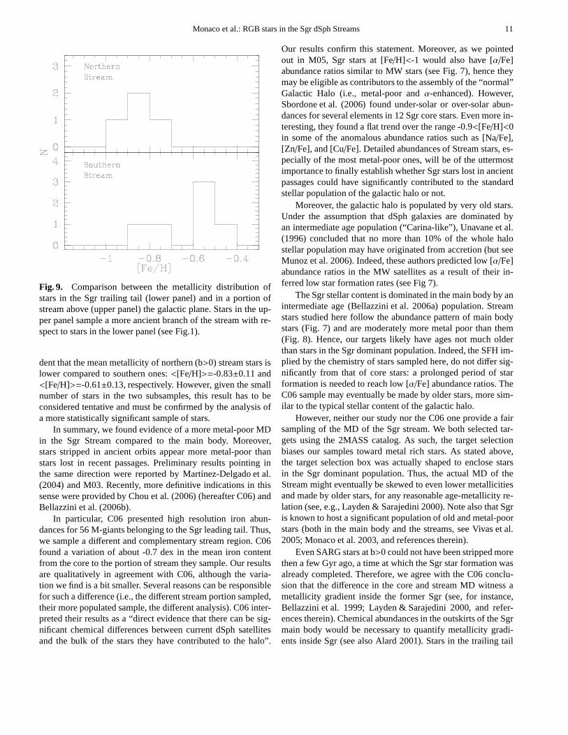
SARG stars sample very different regions of the Stream(see Fig. 1). The sub-sample at negative galactic latitude (starsfrom #1 to #42; b<0 or YS gr,GC >0 in Fig. 1) belongs to theSgr trailing tail in the 80◦ < Λ⊙ < 100◦ region. Hence, theywere probably stripped during the last Sgr orbit. The b>0 sub-sample (stars from #242 to #283) traces, on the other hand,a more ancient episode of tidal stripping. In particular, ac-cording to the Law et al. (2005) model of Sgr disruption, theyshould have been lost three or more orbits ago (i.e.,>2-3 Gyrago). In Fig. 9 we plot the two sub-samples MD. It is evi-

Monaco et al.: RGB stars in the Sgr dSph Streams 11

Fig. 9. Comparison between the metallicity distribution ofstars in the Sgr trailing tail (lower panel) and in a portion ofstream above (upper panel) the galactic plane. Stars in the up-per panel sample a more ancient branch of the stream with re-spect to stars in the lower panel (see Fig.1).

dent that the mean metallicity of northern (b>0) stream stars islower compared to southern ones:<[Fe/H]>=-0.83±0.11 and<[Fe/H]>=-0.61±0.13, respectively. However, given the smallnumber of stars in the two subsamples, this result has to beconsidered tentative and must be confirmed by the analysis ofa more statistically significant sample of stars.

In summary, we found evidence of a more metal-poor MDin the Sgr Stream compared to the main body. Moreover,stars stripped in ancient orbits appear more metal-poor thanstars lost in recent passages. Preliminary results pointing inthe same direction were reported by Martınez-Delgado et al.(2004) and M03. Recently, more definitive indications in thissense were provided by Chou et al. (2006) (hereafter C06) andBellazzini et al. (2006b).

In particular, C06 presented high resolution iron abun-dances for 56 M-giants belonging to the Sgr leading tail. Thus,we sample a different and complementary stream region. C06found a variation of about -0.7 dex in the mean iron contentfrom the core to the portion of stream they sample. Our resultsare qualitatively in agreement with C06, although the varia-tion we find is a bit smaller. Several reasons can be responsiblefor such a difference (i.e., the different stream portion sampled,their more populated sample, the different analysis). C06 inter-preted their results as a “direct evidence that there can be sig-nificant chemical differences between current dSph satellitesand the bulk of the stars they have contributed to the halo”.

Our results confirm this statement. Moreover, as we pointedout in M05, Sgr stars at [Fe/H]<-1 would also have [α/Fe]abundance ratios similar to MW stars (see Fig. 7), hence theymay be eligible as contributors to the assembly of the “normal”Galactic Halo (i.e., metal-poor andα-enhanced). However,Sbordone et al. (2006) found under-solar or over-solar abun-dances for several elements in 12 Sgr core stars. Even more in-teresting, they found a flat trend over the range -0.9<[Fe/H]<0in some of the anomalous abundance ratios such as [Na/Fe],[Zn/Fe], and [Cu/Fe]. Detailed abundances of Stream stars, es-pecially of the most metal-poor ones, will be of the uttermostimportance to finally establish whether Sgr stars lost in ancientpassages could have significantly contributed to the standardstellar population of the galactic halo or not.

Moreover, the galactic halo is populated by very old stars.Under the assumption that dSph galaxies are dominated byan intermediate age population (“Carina-like”), Unavane et al.(1996) concluded that no more than 10% of the whole halostellar population may have originated from accretion (butseeMunoz et al. 2006). Indeed, these authors predicted low [α/Fe]abundance ratios in the MW satellites as a result of their in-ferred low star formation rates (see Fig 7).

The Sgr stellar content is dominated in the main body by anintermediate age (Bellazzini et al. 2006a) population. Streamstars studied here follow the abundance pattern of main bodystars (Fig. 7) and are moderately more metal poor than them(Fig. 8). Hence, our targets likely have ages not much olderthan stars in the Sgr dominant population. Indeed, the SFH im-plied by the chemistry of stars sampled here, do not differ sig-nificantly from that of core stars: a prolonged period of starformation is needed to reach low [α/Fe] abundance ratios. TheC06 sample may eventually be made by older stars, more sim-ilar to the typical stellar content of the galactic halo.

However, neither our study nor the C06 one provide a fairsampling of the MD of the Sgr stream. We both selected tar-gets using the 2MASS catalog. As such, the target selectionbiases our samples toward metal rich stars. As stated above,the target selection box was actually shaped to enclose starsin the Sgr dominant population. Thus, the actual MD of theStream might eventually be skewed to even lower metallicitiesand made by older stars, for any reasonable age-metallicityre-lation (see, e.g., Layden & Sarajedini 2000). Note also thatSgris known to host a significant population of old and metal-poorstars (both in the main body and the streams, see Vivas et al.2005; Monaco et al. 2003, and references therein).

Even SARG stars at b>0 could not have been stripped morethen a few Gyr ago, a time at which the Sgr star formation wasalready completed. Therefore, we agree with the C06 conclu-sion that the difference in the core and stream MD witness ametallicity gradient inside the former Sgr (see, for instance,Bellazzini et al. 1999; Layden & Sarajedini 2000, and refer-ences therein). Chemical abundances in the outskirts of theSgrmain body would be necessary to quantify metallicity gradi-ents inside Sgr (see also Alard 2001). Stars in the trailing tail

12 Monaco et al.: RGB stars in the Sgr dSph Streams

(lower panel in Fig. 9) are only mildly more metal poor thancore ones (upper panel in Fig. 8). Hence, eventually, stars lyingin the outer Sgr core and in the trailing tail might not presentany chemical difference.

Indeed, the great majority of the MW satellites containpopulations of old stars, either dominant or not. It appearsa general tendency of the most metal-poor populations indSphs to be less concentrated with respect to the other popu-lations hosted (Munoz et al. 2006; Tolstoy et al. 2004, and ref-erences therein). This characteristic might favor the preferentialstripping of metal-poor stars during tidal interactions betweendSphs and the MW.

8. Conclusions

The Sgr SFH, its dynamical status and orbital evolution areconstrained by the stellar populations hosted both in the mainbody and in the tidal streams of this disrupting galaxy. In thispaper we presented radial velocities and chemical abundances(Fe, Mg, Ca) for a sample of stars belonging to the Sgr tidalstreams. In particular, we presented the firstα-element abun-dances ever obtained for stars in the Sgr stream. The main re-sults obtained can be summarized as follows:

– The velocity dispersion of the Sgr trailing tail (8.3 kms−1)is significantly lower than in the main body (11.2 kms−1).

– Stream stars follow the same distinct trend described bystars in the Sgr main body in the [Fe/H] vs. [α/Fe] plane(Fig. 7).

– Sgr stars are, on average, more metal-poor in the Streamthan in the core (Fig. 8).

– Stars belonging to more ancient wraps of the Streams aremore metal-poor (Fig. 9). This result was obtained compar-ing the MD of stars belonging to two different wraps of theStream. However, given the limited number of stars in thetwo subsamples (4 and 6), this latter result has to be con-sidered tentative.

Acknowledgements.We are grateful to A. Magazzu for hishelp in preparing the SARG observations. We also thank theLa Silla SciOps department for their help in dealing with theHARPS spectra. Part of the data analysis has been performedusing software developed by P. Montegriffo at the INAF -Osservatorio Astronomico di Bologna. The routines available athttp://www.astro.virginia.edu/∼srm4n/Sgr/ were used to derive coor-dinates in the Sgr orbital plane. We acknowledge support from theMIUR/PRIN 2004025729, the INAF/PRIN05 CRA 1.06.08.02 and theINAF/PRIN05 CRA 1.06.08.03. PB also acknowledges support fromEU contract MEXT-CT-2004-014265 (CIFIST).

References

Alard, C. 2001, A&A, 377, 389Alonso, A., Arribas, S., & Martınez-Roger, C. 1999, A&AS,

140, 261

Bean, J. L., Sneden, C., Hauschildt, P. H., Johns-Krull, C. M.,& Benedict, G. F. 2006, ApJ, in press (astro-ph/0608093)

Bellazzini, M., Ferraro, F.R., Buonanno, R., 1999, MNRAS,307, 619

Bellazzini, M., Correnti, M., Ferraro, F. R., Monaco, L., &Montegriffo, P. 2006a, A&A, 446, L1

Bellazzini, M. , Newberg, H.J. , Correnti, M. , Ferraro, F.R.,Monaco, L. 2006b, A&A, 475, L21

Belokurov, V., et al. 2006a, ApJ, Letters submitted(astro-ph/0605705)

Belokurov, V., et al. 2006b, ApJ, 642, L137Bertone, E., Buzzoni, A., Chavez, M., Rodriguez-Merino, L.H.

2004, AJ, 128, 829Bonifacio P., Hill V., Molaro P., Pasquini L., Di Marcantonio

P., Santin P. 2000, A&A, 359, 663Bonifacio, P., Sbordone, L., Marconi, G., Pasquini, L., & Hill,

V. 2004, A&A, 414, 503 (B04)Chou, M.-Y., Majewski, S.R., Cunha, K., et al., 2006, ApJ

Letters, submitted (C06; astro-ph/0605101)Duffau, S., Zinn, R., Vivas, A. K., Carraro, G., Mendez, R. A.,

Winnick, R., & Gallart, C. 2006, ApJ, 636, L97Dohm-Palmer, R. C., et al. 2001, ApJ, 555, L37Fuhr, J.R., Martin, G.A., and Wiese, W.L. 1988.

J.Phys.Chem.Ref.Data 17, Suppl. 4. (FMW)Fuhr, J.R. and Wiese, W.L., NIST Atomic Transition

Probability Tables, CRC Handbook of Chemistry & Physics,77th Edition, D. R. Lide, Ed., CRC Press, Inc., Boca Raton,FL, 1996 (NIST).

Girardi, L., Bertelli, G., Bressan, A., Chiosi, C., Groenewegen,M. A. T., Marigo, P., Salasnich, B., & Weiss, A. 2002, A&A,391, 195

Gratton, R. G., Carretta, E., Claudi, R., Lucatello, S., &Barbieri, M. 2003, A&A, 404, 187 (G03)

Hargreaves, J. C., Gilmore, G., & Annan, J. D. 1996, MNRAS,279, 108

Helmi, A., & White, S. D. M. 1999, MNRAS, 307, 495Ibata, R.A., Wyse, R.F.G., Gilmore, G., Irwin, M.J., & Suntzeff,

N.B., 1997, AJ, 113, 634Ibata, R. A., Gilmore, G., & Irwin, M. J. 1994, Nature, 370,

194Kurucz, R.L. 1988, Trans. IAU, XXB, M. McNally, ed.,

Dordrecht: Kluwer, p. 168 (K88)Kurucz, R. L. 1993a, CD-ROM 13,

18 http://kurucz.harvard.eduKurucz, R. 1993b, Opacities for Stellar Atmospheres.

Kurucz CD-ROM No. 2–12 Cambridge, Mass.:Smithsonian Astrophysical Observatory, 1993.http://kurucz.harvard.edu/opacities.html

Kurucz, R. 1994, Atomic Data for Fe and Ni. Kurucz CD-ROM No. 22. Cambridge, Mass.: Smithsonian AstrophysicalObservatory, 1994., 22 (K94)

Law, D. R., Johnston, K. V., & Majewski, S. R. 2005, ApJ, 619,807

Layden, A. C., & Sarajedini, A. 2000, AJ, 119, 1760

Monaco et al.: RGB stars in the Sgr dSph Streams 13

Majewski S.R., Skrutskie M.F., Weinberg M.D., OstheimerJ.C., 2003, ApJ, 599, 1082 (M03)

Majewski, S. R., et al. 2004, AJ, 128, 245 (M04)Marconi, G., Buonanno, R., Castellani, M., Iannicola, G.,

Molaro, P., Pasquini, L., & Pulone, L. 1998, A&A, 330, 453Martin, G.A., Fuhr, J.R., and Wiese, W.L. 1988.

J.Phys.Chem.Ref.Data 17, Suppl. 3. (MFW)Martınez-Delgado, D., Gomez-Flechoso, M.A., Aparicio, A.,

& Carrera, R. 2004, ApJ, 601, 242McWilliam, A., & Smecker-Hane, T. A. 2005, ApJ, 622, L29McWilliam, A., Rich, R. M., & Smecker-Hane, T. A. 2003,

ApJ, 592, L21Monaco L., Ferraro F.R., Bellazzini M., Pancino E. 2002, ApJ,

578, L47Monaco L., Bellazzini M., Ferraro F.R., Pancino E., 2003, ApJ,

597, L25Monaco, L., Bellazzini, M., Ferraro, F. R., & Pancino, E. 2004,

MNRAS, 353, 874Monaco, L., Bellazzini, M., Bonifacio, P., Ferraro, F. R.,

Marconi, G., Pancino, E., Sbordone, L., & Zaggia, S. 2005,A&A, 441, 141 (M05)

Munoz, R.R. et al. 2006, ApJ, 649, 201 (M06)Newberg, H. J., et al. 2002, ApJ, 569, 245O’Brian, T. R., Wickliffe, M. E., Lawler, J. E., Whaling, J. W.,

& Brault, W. 1991, Optical Society of America Journal BOptical Physics, 8, 1185 (O)

Olszewski, E. W., Pryor, C., & Armandroff, T. E. 1996, AJ,111, 750

Robertson B., Bullock J.S., Font A.S., Johnston K.V.,Hernquist L., 2005, ApJ, 632, 872

Sbordone, L., Bonifacio, P., Castelli, F., & Kurucz, R. L. 2004,Memorie della Societa Astronomica Italiana Supplement, 5,93

Sbordone, L., Bonifacio, P., Buonanno, R., Marconi,G. ,Monaco, L., & Zaggia, S. 2006, A&A, submitted

Schlegel, D. J., Finkbeiner, D. P., & Davis, M. 1998, ApJ, 500,525

Smith, G., & Raggett, D. S. J. 1981, Journal of Physics BAtomic Molecular Physics, 14, 4015 (SR)

Tolstoy, E., et al. 2004, ApJ, 617, L119Unavane, M., Wyse, R. F. G., & Gilmore, G. 1996, MNRAS,

278, 727Valenti, J. A., Piskunov, N., & Johns-Krull, C. M. 1998, ApJ,

498, 851Venn, K. A., Irwin, M., Shetrone, M. D., Tout, C. A., Hill, V.,

& Tolstoy, E. 2004, AJ, 128, 1177Vivas, A. K., Zinn, R., & Gallart, C. 2005, AJ, 129, 189White, S. D. M., & Rees, M. J. 1978, MNRAS, 183, 341Wiese, W.L., Smith, M.W., and Miles, B.M. 1969, NSRDS-

NBS 22. (NBS)

Appendix A: Individual line data

The following tables report the line list and adopted atomicpa-rameters for the program stars. The measured equivalent widthand the corresponding abundance obtained for each line arealso reported.

List of Objects

‘Sgr dSph’ on page 1‘2MASS J00170214+0104165’ on page 2‘1’ on page 2‘2MASS J01225543+0451341’ on page 2‘19’ on page 2‘2MASS J01295300+0055392’ on page 2‘23’ on page 2‘2MASS J01305453+0351575’ on page 2‘25’ on page 2‘2MASS J01492111+0231536’ on page 2‘39’ on page 2‘2MASS J01520195+0020525’ on page 2‘42’ on page 2‘2MASS J02224517+0039362’ on page 2‘77’ on page 2‘2MASS J08491184+4819380’ on page 2‘232’ on page 2‘2MASS J09193349+4350034’ on page 2‘242’ on page 2‘2MASS J10055844+3132597’ on page 2‘260’ on page 2‘2MASS J10413374+4033099’ on page 2‘278’ on page 2‘2MASS J10472976+2339508’ on page 2‘281’ on page 2‘2MASS J10504744+2748542’ on page 2‘283’ on page 2‘2MASS J13091343+1215502’ on page 2‘465’ on page 2‘2MASS J14340509+0936258’ on page 2‘677’ on page 2‘2MASS J09364419+0704484’ on page 2‘452892’ on page 2‘2MASS J09453656+0937568’ on page 2‘459992’ on page 2‘2MASS J09564707+0645292’ on page 2‘452060’ on page 2‘2MASS J11345053-0700511’ on page 2‘421173’ on page 2‘2MASS J11554802-0339068’ on page 2‘427535’ on page 2‘2MASS J14112205-0610129’ on page 2‘423286’ on page 2‘2MASS J00035283-1940468’ on page 2‘1005’ on page 2

14 Monaco et al.: RGB stars in the Sgr dSph Streams

‘2MASS J00131891-2301528’ on page 2‘1006’ on page 2‘2MASS J00135624-1721554’ on page 2‘1007’ on page 2‘2MASS J00223563-0512079’ on page 2‘1008’ on page 2‘2MASS J00264668-1526427’ on page 2‘1009’ on page 2‘2MASS J00321654-1851113’ on page 2‘1010’ on page 2‘2MASS J00390964-1322429’ on page 2‘1011’ on page 2‘2MASS J00464414-0659259’ on page 2‘1013’ on page 2‘2MASS J00480460-1131551’ on page 2‘1014’ on page 2‘2MASS J00522982-1518360’ on page 2‘1015’ on page 2‘2MASS J00532013-0529477’ on page 2‘1016’ on page 2‘2MASS J00542073-0449174’ on page 2‘1017’ on page 2‘2MASS J00563325-2154386’ on page 2‘1018’ on page 2‘2MASS J01011934-1536343’ on page 2‘1019’ on page 2‘2MASS J01015376-1015085’ on page 2‘1020’ on page 2‘2MASS J01091912-1508157’ on page 2‘1022’ on page 2‘2MASS J01212317-1036096’ on page 2‘1025’ on page 2‘2MASS J01282756-0505173’ on page 2‘1028’ on page 2‘2MASS J01512105-0727451’ on page 2‘1034’ on page 2‘2MASS J01574156-1709471’ on page 2‘1035’ on page 2‘2MASS J01593606-0801131’ on page 2‘1036’ on page 2‘2MASS J21153360-3530060’ on page 2‘1065’ on page 2‘2MASS J21174714-2432331’ on page 2‘1066’ on page 2‘2MASS J21250780-2747090’ on page 2‘1067’ on page 2‘2MASS J21314538-3513510’ on page 2‘1068’ on page 2‘2MASS J21581991-3406074’ on page 2‘1071’ on page 2‘2MASS J22083965-2812124’ on page 2‘1072’ on page 2‘2MASS J22142679-2306184’ on page 2‘1073’ on page 2

‘2MASS J22264953-3918313’ on page 2‘1075’ on page 2‘2MASS J22373980-2628544’ on page 2‘1076’ on page 2‘2MASS J22392246-2508120’ on page 2‘1077’ on page 2‘2MASS J22442231-3247156’ on page 2‘1078’ on page 2‘2MASS J22561212-2045555’ on page 2‘1080’ on page 2‘2MASS J23194353-1546105’ on page 2‘1082’ on page 2‘2MASS J23212651-2426543’ on page 2‘1083’ on page 2‘2MASS J23241474-2750339’ on page 2‘1084’ on page 2‘2MASS J23262366-2500371’ on page 2‘1085’ on page 2‘2MASS J23293008-2458096’ on page 2‘1086’ on page 2‘2MASS J23295478-2051034’ on page 2‘1087’ on page 2‘2MASS J23303457-1607474’ on page 2‘1088’ on page 2‘2MASS J23430789-2358264’ on page 2‘1089’ on page 2‘2MASS J23454168-2644555’ on page 2‘1090’ on page 2‘2MASS J23503612-2002156’ on page 2‘1091’ on page 2‘2MASS J23531941-2050407’ on page 2‘1092’ on page 2‘2MASS J23563742-2347116’ on page 2‘1093’ on page 2‘2MASS J23565416-1906094’ on page 2‘1094’ on page 2‘465’ on page 3‘1006’ on page 3‘1022’ on page 3‘1083’ on page 3‘1006’ on page 3‘459992’ on page 4‘1006’ on page 5‘1006’ on page 5‘1022’ on page 5‘1083’ on page 5‘1006’ on page 5‘1022’ on page 5‘1083’ on page 5‘1006’ on page 6‘1022’ on page 6‘1083’ on page 6‘1006’ on page 6‘1’ on page 7

Monaco et al.: RGB stars in the Sgr dSph Streams 15

‘77’ on page 7‘232’ on page 7‘283’ on page 7‘260’ on page 7‘242’ on page 7‘42’ on page 7‘19’ on page 7‘77’ on page 8‘232’ on page 8‘242’ on page 8‘232’ on page 8‘77’ on page 8‘242’ on page 8‘77’ on page 8‘242’ on page 8‘1’ on page 9‘19’ on page 9‘23’ on page 9‘25’ on page 9‘39’ on page 9‘42’ on page 9‘77’ on page 9‘232’ on page 9‘242’ on page 9‘278’ on page 9‘281’ on page 9‘283’ on page 9‘1’ on page 9‘19’ on page 9‘23’ on page 9‘25’ on page 9‘39’ on page 9‘42’ on page 9‘77’ on page 9‘232’ on page 9‘242’ on page 9‘278’ on page 9‘281’ on page 9‘283’ on page 9‘77’ on page 9‘232’ on page 9‘1’ on page 9‘1’ on page 9‘19’ on page 9‘23’ on page 9‘25’ on page 9‘39’ on page 9‘42’ on page 9‘77’ on page 9‘232’ on page 9‘242’ on page 9‘278’ on page 9‘281’ on page 9‘283’ on page 9

‘19’ on page 9‘1’ on page 10‘42’ on page 10‘242’ on page 10‘283’ on page 10‘1’ on page 16‘19’ on page 16‘23’ on page 16‘25’ on page 16‘39’ on page 17‘42’ on page 17‘77’ on page 17‘232’ on page 17‘242’ on page 18‘278’ on page 18‘281’ on page 18‘283’ on page 18

16 Monaco et al.: RGB stars in the Sgr dSph Streams

Table A.1.Line list and adopted atomic parameters for the program stars. The measured equivalent width and the correspondingabundance obtained for each line are also reported.

Ion λ log gf source of EW ǫ EW ǫ EW (pm) ǫ EW ǫ

(nm) log gf (pm) (pm) (pm) (pm)(see notes) 1 19 23 25

Fe I 585.5076 -1.76 FMW – – – – 5.09 7.283 – –Fe I 588.3817 -1.36 FMW – – 9.47 6.640 12.15 7.151 12.15 7.151Fe I 595.2718 -1.44 FMW 12.89 7.324 9.27 6.719 12.70 7.360 7.62 6.491Fe I 602.7051 -1.21 FMW 10.52 6.818 10.78 6.861 9.28 6.661 11.17 6.981Fe I 605.6005 -0.46 FMW 9.18 6.795 7.43 6.517 8.31 6.692 8.08 6.654Fe I 609.6664 -1.93 FMW – – 6.05 6.707 6.19 6.748 9.76 7.324Fe I 615.1617 -3.30 FMW 18.60 7.279 17.79 7.166 19.23 7.439 14.43 6.730Fe I 622.6734 -2.22 FMW – – 8.13 7.162 – – – –Fe I 651.8366 -2.75 FMW 11.27 6.580 13.18 6.868 11.94 6.734 13.97 7.052Fe I 659.7559 -1.07 FMW 7.05 7.145 4.28 6.695 7.44 7.233 6.97 7.158Fe I 670.3566 -3.16 FMW 9.40 6.598 9.03 6.546 13.87 7.319 – –Fe I 673.9521 -4.95 FMW 11.68 6.885 10.37 6.704 11.27 6.873 12.58 7.066Fe I 674.6954 -4.35 FMW – – 4.74 6.923 6.99 7.254 5.55 7.052Fe I 679.3258 -2.47 FMW 3.75 6.989 3.12 6.872 – – 5.08 7.224

Fe I 595.6694 -4.60 FMW – – 20.24 7.026 20.59 7.225 – –Fe I 595.8333 -4.42 K94 9.36 7.040 10.36 7.187 – – – –Fe I 602.4058 -0.12 FMW 17.44 7.486 14.06 6.988 11.71 6.661 13.83 7.016Fe I 606.5482 -1.53 FMW 25.18 6.994 21.92 6.673 20.84 6.620 23.89 6.938Fe I 624.6318 -0.96 FMW 19.52 7.245 14.82 6.548 16.37 6.872 15.48 6.729Fe I 625.2555 -1.69 FMW – – 23.13 6.629 22.50 6.631 23.18 6.700Fe I 629.7793 -2.74 FMW – – 18.29 6.714 19.64 6.967 17.54 6.685Fe I 630.1500 -0.67 K94 – – 14.88 6.335 15.81 6.560 – –Fe I 630.2494 -1.13 K94 12.39 6.442 13.55 6.629 17.73 7.360 16.04 7.106Fe I 632.2685 -2.43 FMW 15.38 6.551 14.90 6.476 17.76 7.001 17.16 6.909Fe I 633.5330 -2.23 FMW 25.32 6.923 22.29 6.643 22.59 6.733 21.80 6.654Fe I 633.6823 -1.05 FMW 19.20 7.397 16.53 7.016 16.27 7.054 15.30 6.900Fe I 657.4227 -5.04 FMW 18.29 7.107 17.54 6.990 17.25 7.037 – –Fe I 659.3870 -2.42 FMW 21.62 7.152 19.62 6.893 20.61 7.106 18.94 6.882Fe I 664.8080 -5.29 K94 – – 11.18 6.325 – – 12.35 6.538Fe I 671.0318 -4.88 FMW 11.55 6.686 13.05 6.900 10.81 6.627 12.96 6.946Fe I 675.0152 -2.62 FMW 20.26 7.233 17.74 6.829 18.33 7.024 18.84 7.109Fe I 680.6843 -3.21 FMW 10.46 6.744 11.22 6.853 13.74 7.287 13.32 7.222Fe I 683.9830 -3.45 FMW 12.10 6.963 11.26 6.842 14.43 7.374 12.47 7.071Fe I 722.3658 -2.21 O 16.91 7.048 – – 18.22 7.291 13.20 6.584Fe I 756.8899 -0.87 K94 13.63 7.114 11.48 6.809 12.45 7.000 13.39 7.136Fe I 758.3788 -1.99 FMW 15.44 6.590 17.23 6.836 16.66 6.829 19.54 7.208Fe I 774.8269 -1.76 FMW 21.39 6.989 17.32 6.488 19.73 6.868 19.91 6.890Fe I 783.2196 -0.02 K94 15.37 6.719 14.80 6.641 – – 16.70 6.962

Mg I 552.8405 -0.52 G03 29.56 7.055 22.58 6.631 23.07 6.697 25.11 6.831Mg I 571.1088 -1.73 G03 13.92 6.848 11.55 6.519 14.39 6.956 15.21 7.069Mg I 631.8717 -1.94 G03 5.87 7.037 4.83 6.884 – – 9.15 7.521Mg I 631.9237 -2.16 G03 6.78 7.386 5.26 7.169 – – 5.28 7.183

Ca I 585.7451 0.24 SR 18.52 5.373 17.00 5.171 19.85 5.596 – –Ca I 586.7562 -1.49 G03 6.07 5.356 6.59 5.424 6.59 5.439 7.31 5.535Ca I 643.9075 0.39 SR – – 22.20 5.111 24.50 5.474 25.39 5.565Ca I 645.5558 -1.29 SR 14.51 5.654 12.81 5.403 13.25 5.523 12.34 5.385Ca I 649.3781 -0.11 SR 21.04 5.423 21.85 5.533 23.21 5.795 22.20 5.669Ca I 649.9650 -0.82 SR 14.09 5.110 16.81 5.512 – – 16.02 5.466Ca I 650.8850 -2.11 NBS 6.57 5.402 4.86 5.180 6.27 5.377 5.66 5.297Ca I 714.8150 0.21 K88 21.33 5.288 24.59 5.694 21.31 5.367 24.13 5.721

FMW – Fuhr et al. (1988)G03 – Gratton et al. (2003)SR – Smith et al. (1981)NBS – Wiese et al. (1969)MFW – Martin et al. (1988)O – O’Brian et al. (1991)K88 – Kurucz (1988)K94 – Kurucz (1994)

Monaco et al.: RGB stars in the Sgr dSph Streams 17

Table A.1.Line list and adopted atomic parameters for the program stars. The measured equivalent width and the correspondingabundance obtained for each line are also reported (continued).

Ion λ log gf source of EW ǫ EW ǫ EW (pm) ǫ EW ǫ

(nm) log gf (pm) (pm) (pm) (pm)(see notes) 39 42 77 232

Fe I 585.5076 -1.76 FMW – – – – 3.42 6.991Fe I 588.3817 -1.36 FMW 10.18 6.982 11.63 6.999 8.12 6.496 – –Fe I 595.2718 -1.44 FMW 8.66 6.795 – – 6.50 6.337 9.61 6.774Fe I 602.7051 -1.21 FMW 9.63 6.879 8.97 6.570 11.12 7.032 10.26 6.776Fe I 605.6005 -0.46 FMW 9.97 7.127 8.48 6.684 8.85 6.822 – –Fe I 609.6664 -1.93 FMW – – 6.51 6.777 – – – –Fe I 615.1617 -3.30 FMW 16.41 7.282 14.11 6.610 12.70 6.517 – –Fe I 622.6734 -2.22 FMW 6.88 7.085 7.55 7.075 7.43 7.115 – –Fe I 651.8366 -2.75 FMW 13.11 7.126 13.62 6.934 13.14 6.987 – –Fe I 659.7559 -1.07 FMW 8.21 7.473 5.27 6.862 4.66 6.790 8.62 7.387Fe I 670.3566 -3.16 FMW 14.04 7.574 9.33 6.589 8.65 6.558 12.34 7.025Fe I 673.9521 -4.95 FMW 10.13 6.849 9.69 6.614 6.12 6.188 10.51 6.723Fe I 674.6954 -4.35 FMW 4.59 6.946 2.75 6.588 – – 7.66 7.324Fe I 679.3258 -2.47 FMW 4.52 7.175 – – 2.28 6.699 3.49 6.942

Fe I 595.6694 -4.60 FMW – – – – – – 18.39 6.684Fe I 595.8333 -4.42 K94 – – 9.58 7.072 8.90 7.045 – –Fe I 602.4058 -0.12 FMW 12.20 6.947 14.65 7.081 11.99 6.772 – –Fe I 606.5482 -1.53 FMW 23.51 7.047 24.52 6.935 18.41 6.380 – –Fe I 624.6318 -0.96 FMW 16.04 7.065 13.81 6.383 12.91 6.372 18.17 7.060Fe I 625.2555 -1.69 FMW 24.06 6.941 20.18 6.272 20.73 6.503 – –Fe I 629.7793 -2.74 FMW 18.36 7.022 16.60 6.474 17.70 6.784 21.40 7.103Fe I 630.1500 -0.67 K94 15.46 6.749 – – – – 20.32 7.119Fe I 630.2494 -1.13 K94 11.82 6.609 14.14 6.724 11.32 6.384 15.62 6.961Fe I 632.2685 -2.43 FMW 16.06 6.995 15.42 6.557 14.43 6.553 20.26 7.268Fe I 633.5330 -2.23 FMW 22.17 6.862 20.51 6.443 21.28 6.664 25.64 6.949Fe I 633.6823 -1.05 FMW 12.76 6.699 15.87 6.914 14.54 6.853 15.85 6.911Fe I 657.4227 -5.04 FMW 17.28 7.375 15.65 6.694 15.35 6.809 17.16 6.928Fe I 659.3870 -2.42 FMW 18.75 7.107 18.63 6.751 17.99 6.830 20.47 7.006Fe I 664.8080 -5.29 K94 – – – – – – – –Fe I 671.0318 -4.88 FMW 12.46 7.067 11.02 6.614 9.63 6.499 13.63 6.985Fe I 675.0152 -2.62 FMW 17.57 7.223 17.65 6.814 15.25 6.596 17.93 6.860Fe I 680.6843 -3.21 FMW 12.14 7.230 8.98 6.536 11.60 7.012 15.19 7.440Fe I 683.9830 -3.45 FMW 10.49 6.927 10.57 6.743 10.53 6.826 12.84 7.070Fe I 722.3658 -2.21 O 12.18 6.612 16.80 7.032 13.09 6.628 – –Fe I 756.8899 -0.87 K94 11.28 6.985 9.63 6.543 9.38 6.581 14.54 7.242Fe I 758.3788 -1.99 FMW 16.86 7.084 13.43 6.310 17.23 6.984 18.67 7.025Fe I 774.8269 -1.76 FMW 17.63 6.825 19.17 6.725 – – 21.35 6.985Fe I 783.2196 -0.02 K94 15.51 7.000 14.60 6.613 11.90 6.334 15.55 6.744

Mg I 552.8405 -0.52 G03 21.73 6.681 – – 25.85 6.904 35.63 7.285Mg I 571.1088 -1.73 G03 11.84 6.714 13.58 6.801 14.69 7.043 21.27 7.702Mg I 631.8717 -1.94 G03 5.25 6.993 5.78 7.024 5.58 7.019 8.01 7.337Mg I 631.9237 -2.16 G03 – – 3.91 6.957 4.32 7.040 9.10 7.709

Ca I 585.7451 0.24 SR – – 18.84 5.412 – – – –Ca I 586.7562 -1.49 G03 6.30 5.452 6.57 5.421 6.05 5.380 9.29 5.778Ca I 643.9075 0.39 SR 23.35 5.560 26.09 5.566 24.89 5.582 28.62 5.791Ca I 645.5558 -1.29 SR 11.66 5.445 10.51 5.084 11.26 5.273 14.07 5.588Ca I 649.3781 -0.11 SR 21.88 5.869 18.99 5.127 24.52 6.011 29.15 6.299Ca I 649.9650 -0.82 SR 15.63 5.644 18.92 5.829 16.29 5.587 19.82 5.961Ca I 650.8850 -2.11 NBS 5.31 5.286 4.92 5.188 10.40 5.961 12.66 6.198Ca I 714.8150 0.21 K88 21.63 5.668 24.18 5.646 – – 27.45 5.991

FMW – Fuhr et al. (1988)G03 – Gratton et al. (2003)SR – Smith et al. (1981)NBS – Wiese et al. (1969)MFW – Martin et al. (1988)O – O’Brian et al. (1991)K88 – Kurucz (1988)K94 – Kurucz (1994)

18 Monaco et al.: RGB stars in the Sgr dSph Streams

Table A.1.Line list and adopted atomic parameters for the program stars. The measured equivalent width and the correspondingabundance obtained for each line are also reported (continued).

Ion λ log gf source of EW ǫ EW ǫ EW (pm) ǫ EW ǫ

(nm) log gf (pm) (pm) (pm) (pm)(see notes) 242 278 281 283

Fe I 585.5076 -1.76 FMW 5.72 7.352 – – – – – –Fe I 588.3817 -1.36 FMW 11.53 6.927 9.43 6.677 – – – –Fe I 595.2718 -1.44 FMW – – – – 7.76 6.455 7.05 6.400Fe I 602.7051 -1.21 FMW 10.49 6.768 – – – – 10.04 6.787Fe I 605.6005 -0.46 FMW 10.37 6.943 – – – – 9.90 6.956Fe I 609.6664 -1.93 FMW 7.12 6.846 – – 4.76 6.494 – –Fe I 615.1617 -3.30 FMW – – – – – – – –Fe I 622.6734 -2.22 FMW – – – – – – – –Fe I 651.8366 -2.75 FMW 14.65 7.025 12.76 6.863 9.72 6.320 – –Fe I 659.7559 -1.07 FMW 5.24 6.842 – – – – – –Fe I 670.3566 -3.16 FMW 12.66 7.019 11.00 6.873 10.05 6.655 11.96 7.021Fe I 673.9521 -4.95 FMW 10.45 6.679 9.00 6.553 7.72 6.342 13.07 7.141Fe I 674.6954 -4.35 FMW – – – – 5.22 6.981 – –Fe I 679.3258 -2.47 FMW 4.91 7.170 – – – – 3.55 6.962

Fe I 595.6694 -4.60 FMW 16.41 6.242 – – 19.00 6.683 19.00 6.919Fe I 595.8333 -4.42 K94 7.40 6.747 – – 8.38 6.876 6.24 6.627Fe I 602.4058 -0.12 FMW 12.83 6.728 – – 12.05 6.603 10.68 6.486Fe I 606.5482 -1.53 FMW – – 23.45 6.895 21.45 6.542 21.61 6.708Fe I 624.6318 -0.96 FMW 15.55 6.589 – – 15.87 6.639 – –Fe I 625.2555 -1.69 FMW – – 26.25 6.971 – – 24.47 6.823Fe I 629.7793 -2.74 FMW 15.56 6.248 21.39 7.168 – – 15.42 6.369Fe I 630.1500 -0.67 K94 16.14 6.459 15.86 6.568 17.10 6.605 15.84 6.565Fe I 630.2494 -1.13 K94 13.02 6.483 12.69 6.553 12.64 6.425 13.47 6.684Fe I 632.2685 -2.43 FMW 15.12 6.441 15.88 6.708 15.14 6.444 15.07 6.578Fe I 633.5330 -2.23 FMW – – 24.91 6.940 20.67 6.391 22.60 6.734Fe I 633.6823 -1.05 FMW 13.71 6.505 – – 13.92 6.540 12.88 6.501Fe I 657.4227 -5.04 FMW 14.60 6.471 18.63 7.268 16.10 6.687 15.88 6.810Fe I 659.3870 -2.42 FMW 17.24 6.469 19.73 6.990 17.47 6.503 17.39 6.655Fe I 664.8080 -5.29 K94 – – 11.28 6.383 – – 12.07 6.497Fe I 671.0318 -4.88 FMW 9.44 6.374 9.86 6.493 8.40 6.246 11.996.799Fe I 675.0152 -2.62 FMW 14.22 6.206 16.74 6.758 16.87 6.605 15.44 6.541Fe I 680.6843 -3.21 FMW 11.65 6.869 – – 10.22 6.673 11.97 7.014Fe I 683.9830 -3.45 FMW – – – – – – – –Fe I 722.3658 -2.21 O – – – – 11.75 6.278 12.76 6.520Fe I 756.8899 -0.87 K94 10.44 6.620 – – 8.56 6.361 10.48 6.707Fe I 758.3788 -1.99 FMW 16.06 6.611 – – 14.70 6.429 – –Fe I 774.8269 -1.76 FMW 16.95 6.370 20.60 6.971 19.16 6.652 – –Fe I 783.2196 -0.02 K94 – – – – – – 15.40 6.786

Mg I 552.8405 -0.52 G03 27.28 6.913 23.13 6.701 24.86 6.765 23.99 6.759Mg I 571.1088 -1.73 G03 16.77 7.177 – – 15.06 6.958 13.41 6.819Mg I 631.8717 -1.94 G03 6.01 7.045 5.10 6.935 2.93 6.554 6.12 7.086Mg I 631.9237 -2.16 G03 – – 4.42 7.049 4.60 7.060 4.61 7.079

Ca I 585.7451 0.24 SR – – – – – – – –Ca I 586.7562 -1.49 G03 8.14 5.603 6.08 5.370 8.39 5.658 9.15 5.788Ca I 612.2217 -0.31 NIST – – – – – – 26.64 5.527Ca I 643.9075 0.39 SR 25.02 5.378 24.47 5.471 27.48 5.693 22.89 5.286Ca I 645.5558 -1.29 SR 13.46 5.445 11.82 5.310 15.41 5.788 10.51 5.120Ca I 649.3781 -0.11 SR 21.55 5.408 22.55 5.713 21.13 5.436 – –Ca I 649.9650 -0.82 SR 15.81 5.297 17.32 5.667 14.56 5.179 – –Ca I 650.8850 -2.11 NBS 7.85 5.542 7.30 5.510 9.29 5.742 5.03 5.212Ca I 714.8150 0.21 K88 25.94 5.763 24.47 5.761 22.89 5.486 22.59 5.535

FMW – Fuhr et al. (1988)G03 – Gratton et al. (2003)SR – Smith et al. (1981)NIST – Furh & Wiese (1996)NBS – Wiese et al. (1969)MFW – Martin et al. (1988)O – O’Brian et al. (1991)K88 – Kurucz (1988)K94 – Kurucz (1994)