PEPRESENTATIVE SELECTION OF VARIABLES

by

Robert Arthur Ra1es

Thesis submitted to the Graduate Faculty of the

1 Virginia Polytechnic Institute

in candidacy for the degree of

MASTER OF SCIENCEin

StatisticsI

I

I{ October 1961IA Blacksburg, VirginiaI

I I.

.. Q ...

TABLE OF CONTENTS

Chapter Page

• • • • • • • • • • • • • • • • • • 3

I. THEORY OF REPRESENTATIVE SELECTION . . . . . . . lll•l Notation • • • • • • • • • • • • • • • • •

•1.2Artificial Discriminator and Selection ofVaI°i8,bl€S • • • • • • • • • • • • • • • •

•1.3Representative Selection . .... . .... 15

II. DEMONSTRATION STUDY 1 . . . . . . . . . . . . . . 21

2.1 Description of Data . . . . . . . . . . . . 21L

2.2 Preparation of Data . . . . . . . . . . . . 23

2.3 Factor Analysis . . . . . .·. . . . . . . . 29

2.4 Discriminatory Analysis . . . . . . . . . . 412•5 OI°d€I‘iI°lg • • • • • • • • • •. • • • • • • ••2•6

SGlGCbiOH • • • • • • • • • • • • • • • • • 52

III. DEMONSTRATION STUDY 2 . . . . . . . . . . . . . . 53

3.1 Description of Data . . . . . . . . . . . . 53

3.2 Factor Analysis . . . . . . . . . . . . . . 55

3.3 Discriminatory Analysis . . . . . . . . . . 63

3•l,}. OI°d€I°iI]g • • • • • • • • • • • • • • • • ••3•5

S€lGCtj.ÜH • • • • • • • • • • • • • • • • •

• • • • • • • • • • • • • • • • • •

• • • • • • • • • • • • • • • •

• • • • • • • • • • • • • • • • • • • • • •

. g „

INTRODUCTION

The classical and most frequent use of the discriminantfunction is for the purpose of classification, by obtaining

a combined measurement such that the difference between two

or more groups is as large as possible. The linear dis-

criminant function for the special case of two groups was

first discussed by R. A. Fisher (see [7]). A systematic

generalization of the concept of discriminant functions was

presented by S. N. Roy (see [11]); who utilized the dis-

criminant function for the purpose of constructing tests of

multivariate hypotheses. Discrimination between two groups

has been widely utilized and is now discussed in many

standard textbooks.The discriminant function is a linear combinatien of

the observable variables. we will speak of "observable”

variables, if we can make direct measurements on them. All

combinations into other functions, be they linear combinations

or otherwise, will be referred to as "artificial" variables.

In this sense, the linear discriminant function can be

regarded as an artificial variable, for it represents a

linear combination of the observable ones. Following S. N.

Roy's approach, we may regard, as the discriminant function,

that combination of the observable variables which produces

the largest possible F-ratio between all groups under

investigation. In this general notation, the discriminant

function will be the eigenvector associated with the largest

characteristic root of E°lH, where E is a matrix of sums·of-

squares and products due to error and H is a matrix of sumsof squares and products due to a given hypothesis whichspecifies the groups. A more detailed exposition of thisfact will be presented in Chapter I of this thesis.

The purpose of this thesis is to study the role of the

discriminant function as a basis for selecting variables.Let us assume that we have k groups of experimental units,

and on each experimental unit we make p observations. wewould like to find that linear combination of the variables

which produces a new variable such that the F—ratio betweenthe k groups is a maximum. This linear combination of the

variables is cf course the discriminant function. we may

regard this variable as an artificial variable constructedfrom the observed ones. we may then proceed to obtain thecorrelations of this artificial variable versus each of theobserved variables. This vector of correlations will give us

an idea of the proximity of the discriminant function to each

of the observable variables. If, for example, we find a few

correlations extremely high, say about .80, we can say that

there is hardly any difference between the best discriminator

between the k groups and those particular observed variables.

We can then take the variables which have high correlations

„ 5 -

versus the discriminant function as almost equivalent in dis-

criminatory power to that of the discriminant function itself.

If, in further experimentation, we intend te reduce the number

of variables on which we would like to perform.measurements,

we will of course select those variables which have the

highest correlations (in absolute value) versus the best

discriminator. This technique has been occasionally utilized

for the selection of variables.

The best way to introduce the concept of representative

selection is in the form of an example. Suppose we are

interested in the difference between human beings of different

races. we are not only interested in the physical character-

istics but also, let us say, in their physiological differences,

such as blood pressure, certain chemicals in the blood stream,

respiration rate, etc. Let us assume, then, that we have

three different racial groups and that we make 10 anthropo-

logical measurements, such as general height, weight, arm

length, color of skin, etc., and that we also make l0

measurements on physiological characteristics such as blood

pressure, content of calcium in the blood stream, etc. If

we apply the previously mentioned discriminant function as a

principle of selection, we will only include physical or

anthropological variables in our selected set, because,

naturally, the racial groups differ most strikingly in terms

of physical characteristics. Thus, if we should perform a

„ g -

new set of experiments based only on the reduced set of

variables, we would measure nothing but physical character-

istics. This would completely obliterate any physiological

measurements that we have previously conducted. It is in

this context that the concept of representative selection

enters. we may wish to select subsets out of the whole set

of variables such that all the important common characteris-

tics of the original set of variables are retained. It is

thus necessary to classify the whole set of variables into

certain subsets that belong together.

The classical method of finding subsets of variables

such that they are classified under certain consistent

principles of classification, is the so-called factor analysis

(see [2] and [12]). In factor analysis, or, more generally,

in Dependence Analysis, an attempt is made to explain the

observed dependence among all the variables in terms of a

few outside or artificial variables. These variates,

incidentally, are not linear combinations of the original

variables. This is a very striking difference between factor

analysis and what is known as component analysis, which has

no bearing on the present problem. The method of classifica-

tion of subsets of variables is explained in detail in

Chapter I, where the various preferred solutions of factor

analysis have been explained and defined, and where the role

of the "Simple Structure" as a classification principle is

„ 7 -

outlined. It is then shown that representative selection is

performed in two stages. In the first stage, any group dif-

ferences which may exist are eliminated in that we consider

only the matrix of sums-of—squares and products due to error.

From this matrix we construct a correlation matrix and on the

basis of this correlation matrix we classify the variables

into subsets.In Chapter I the role of the discriminant function as a

basis for the selection of variables, and the principle of

representative selection by factor analysis is explained in

detail. Chapter II presents a detailed demonstration study,

where a factorial structure of the variables is known. It

consists of a sampling experiment in which the variables

have been arranged so as to form a structure in three artifi-

cial variables or factors. Chapter III presents a study of

actual data which are an excerpt from a study on mentally

retarded children, carried out in 1957-60 (see [13]). we

selected three different sets of variables from these;

intelligence measures, straight achievement measures, and

measures of achievement gain in the course of one year. we

were interested in discriminating between twe groups; those

children who stayed in the public school system, and those

students who were transferred to special classes for mentally

retarded children. Previous analysis of these daya showed

that there was a rather striking interaction between the

difference in school types and the age of the subjects, inthat older children in the public education system performedconsiderably better than the older children that had beenreferred to special education classes. The difference wasnot nearly as great in the younger age groups. For thatreason, we had to make three separate studies in investigatingthe discriminant functions and in finding the best representa-tives among the observed variables. A study was made forthe children ll years and younger, between ll and l3 yearsof age, and for the group 13 years of age and older. Therather interesting and somewhat surprising findings of thestudies are mentioned in Chapter III.

In the actual analysis of these data one must make useof algebraic advantages by representing matrices in the

smallest possible form. The details of numerical evaluationsin this case are presented in Chapter II.

For clarification it must be pcinted out that the methodof selecting variables on the basis of their correlations onthe best discriminator does not insure that one will findsubsets of 2, 3, or more variables which produce maximum

F—ratios of all possible doublets, triplets, etc. No methodfor the selection of the best discriminating single variablecan be used for finding, in general, the best two or three,

for the ”best" doublet may not even contain the best singlevariable. For illustration, let us consider the following

example:Let 21 and 22 be two uncorrelated variables, and let6

23 = 21 *422 + u , where u is independent cf 21 and 22 andhas the same variance. Suppose we found, with 21 and 22expressed in standard units, that d = 21 + 22 is the bestdiscriminator between the groups under study in the sensethat this combination of the three variables (21, 22, 23)would produce the highest F—ratio between groups. Thus, thecorrelations would be

21 22 23 d2l 1.000 0.000 .577 .70722 0.000 1.000 .577 .707

23 .577 .577 1.000 .816Clearly, 23 is the best single discriminating variable (itis, except for a relatively small error u, equal to the dis-criminant function itself, even though on the ”partial”regression weights of d on 23 given 21 and 22 it need notappear at all). However, the best pgg; of variables is 2land 22 and does not even contain the best single variable 23 .In fact, the multiple correlations of d on every possiblepair are

R (dj 21, 22) = 1.000

R (dj 21, 23) = .866

R (dj 22, 23) = .866

- lO -

so that 23 is never a member of the best pair.In the method proposed in this thesis the discriminant

function is regarded as some unknown but real latent variable

which produces maximum discrimination, and observable variablesare selected in terms of their eloseness to this ideal under-lying variable. In this sense, it is natural to ask whetherjust one ideal variable would be sufficient to explain thediscrimination, and it is for this reason that the representa-tive selection has been proposed as an extension of this idea.

- ll -

Chapter I: THEORY OF REPRESENTATIVE SELECTION

1.1 Notation

we shall present here some standard notation to facili-

tate reading:

(1.1.1) A' = transpose of a matrix A

(1.1.2) x = column vector; x' = row vector

(1.1.3) E = covariance matrix

(1.1.4) S = maximum—1ikelihood estimate of E

(1.1.5)‘R’=

matrix of correlations in the population

(1.1.6) R = maximum-likelihood estimate of (sample

correlations)

(1.1.7) F (p x k) ¤ maximum-likelihood estimate of the matrix

of correlations between observable and artifi-

cial variates, so-called "factor loadings"

(1.1.8) hiz = sum-of-squares of the i'th row of F, called

"communalities", which are squares of multiple

correlations of each observed variable versus

all artificial variables (factors)

(1.1.9) R (gßg) = matrix of all sample partial corre1a—

tions in a set of variables, g, given another

set,(1.1.10)

Da = diagonal matrix whose elements are al, a2,..., ap

(1.1.11) E = matrix of sums-of—squares and products due to

error

- 12 -

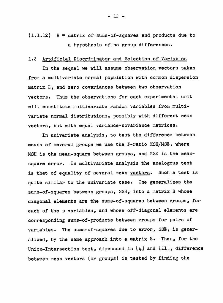
(1.1.12) H = matrix of sums—of-squares and products due to

a hypothesis of no group differences.

1.2 Artificial Discriminator and Selection of Variables

In the sequel we will assume observation vectors takenfrom a multivariate normal population with common dispersion

matrix 2, and zero covariances between two observation

vectors. Thus the observations for each experimental unit

will constitute multivariate random variables from multi-

variate normal distributions, possibly with different mean

vectors, but with equal variance-covariance matrices.In univariate analysis, to test the difference between

means of several groups we use the F-ratio MSH/MSE, where

MSH is the mean-square between groups, and MSE is the mean-

square error. In multivariate analysis the analogous test

is that of equality of several mean vectors. Such a test is

quite similar to the univariate case. One generalizes the

sums-of-squares between groups, SSH, into a matrix H whose

diagonal elements are the sums-of-squares between groups, for

each of the p variables, and whose off-diagonal elements are

corresponding sums-of-products between groups for pairs of

variables. The sums-of-squares due to error, SSE, is gener-

alized, by the same approach into a matrix E. Then, for the

Union-Intersection test, discussed in [A] and [ll], difference

between mean vectors (or groups) is tested by finding the

- 13 -

largest characteristic root of E°lH , (see [8]). What is of

interest here is the eignevector associated with this largest

characteristic root ofE”lH,

i.e., the vector g such that

(1.2.1) E"lH g =·= A. g .This eigenvector g' is called the discriminant functionbetween the groups; more specifically gfg, where g is the

vector of observable variables, is that linear combination of

g which produces maximum separation between mean effects, in

that a univariate F test for the hypothesis of no group dif-

ferences, performed on the artificial variable u will

produce the largest possible F—ratio.

As was stated, the discriminant function is an artificial

variable, u =_gig . In other werds, given a matrix of

observations for n experimental units on p variables, i.e.,

a matrix Z (n x p), and a grouping principle which subdivides

Z into groups Zl (nl x p), Z2 (ng x p), ..., Zk (nk x p), wecan obtain E°lH and hence a discriminant vector g'. Then,

if we form the vector g = Zlä , i.e., a vector with n

elements, the elements ui may be regarded as the response

on that artificial variable u which produces maximum separa-

tion between the k groups.

In this thesis we are interested in interpreting the

artificial variable u . In particular, we would like to find

those variables among the observable set g which are

- lg -

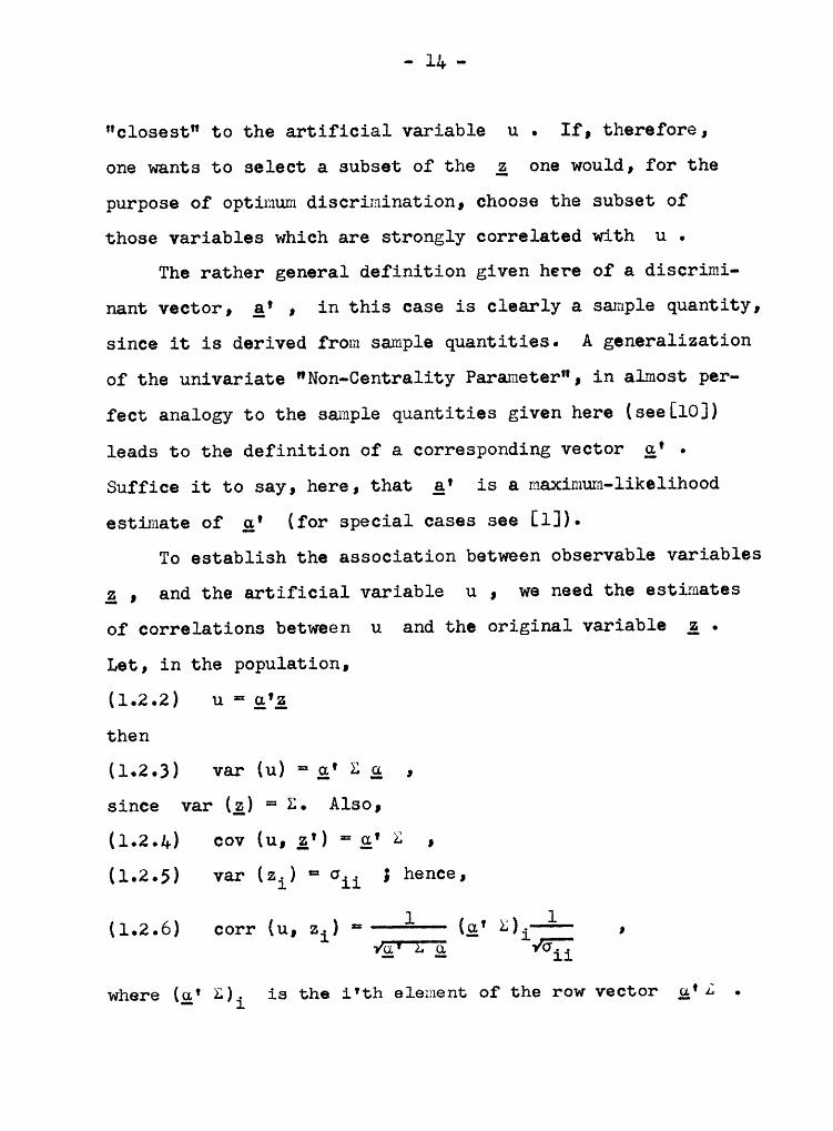
"closest" to the artificial variable u . If, therefore,

one wants to select a subset of the g one would, for the

purpose of optimum discrimination, choose the subset of

those variables which are strongly correlated with u .

The rather general definition given here of a discrimi—

nant vector, gf , in this case is clearly a sample quantity,

since it is derived from sample quantities. A generalization

of the univariate "Non—Centrality Parameter", in almost per-

fect analogy to the sample quantities given here (see[lO])

leads to the definition of a corresponding vector g' .

Suffice it to say, here, that _g' is a maximum—likelihood

estimate of ·g' (for special cases see [1]).

To establish the association between observable variables

g , and the artificial variable u , we need the estimates

of correlations between u and the original variable g .

Let, in the population,

(1.2.2) u ==g_n_'_g_

then

(1.2.3) var (u) =_g' E g ,

since var (3) = Z. Also,(1.2.A) cov (u, g') “_g' E ;

(1.2.5) var (zi) ¤ Gii ; hence,

(1.2.6) corr (u, zi)

(g'where(g' Z)i is the i'th element of the row vector g*2l .

- 15 -

Thus

(l•2•7) corr (u pg') =·——-l———_g* E D „ .’ avm 1/*%Now, the maximum—like1ihood estimate of Ig is a , the

maximum·likelihood estimate of E is é E , and henceas.-—-—-„—•-«•:l° .-l ””‘(1.2.8) I‘ (1.1, Q') 11/—·a' E a¤•¤• -••

‘ {ä' E gp ii

The vector will be used for the purpose of selection of

variables.

1.3 Representative Selection

Given a set of p observable variables, 2l, 22, ..., zp,

we want to subdivide them into subsets. In other words, we

want to find some principle of classification which enables

us to put certain variables into a common class. This task

is usually performed by Factor Analysis (see [2], [9], and

[12]). The purpose of Factor Analysis is the study of

dependence patterns in the variables. This is accomplished

by seeking artificial variables which may explain the depen—

dence among the observable variables. It is well known, in

the theory of partial correlations, that dependence in a set

of variables may be due to the presence of a common outside

.. _‘_é ..

variable. The goal in Factor Analysis is to find one ormore artigicial variables which could explain the dependenceof all the observable variates.* These artificial variablesare described in terms of their correlations with the observ-able ones and these correlations have been called ”factor1oadings”. The artificial variables, Ä , must be determinedin such a way that they ”exp1ain the dependence" in the set

Ä . Hence, if we can find {Ä such that the hypothesis

HO: R (ale) = I is acceptable, the set Ä will serve ourpurpose. The solution of this problem for k factors(k = 1, 2, ...) is given by the relations (see [2])

(1.3.1) (R — F F') Dl/l_hi2 F = F .

Any F satisfying this relation is a matrix of "factor load-

ings” which solves this problem, and hi? is the sum-of-

squares of the i'th row in F and also is the square of the

multiple correlation (in the sample) of the artificial

variables versus the i'th observable variable.

Suppose we choose k = l, 2, 3, ... and, for each choice

of k , find an F satisfying Eguation (1.}.1). Given this

F we can test the hypothesis R’(g)Ä) = I by a test ofpartial independence. It is, [1],

*There is the further attempt analogous to the problem offitting polynomials (see [2]), to keep the number of suchartificial variables or factors as small as possible.

- 17 „

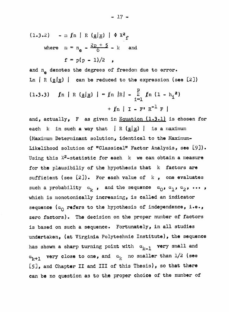
(1-3-2) - m fn I R (ala;) I e xßf

where m = ne - g2Ei—2 - k andf=mp—n& „

and na denotes the degrees of freedom due to errcr.

Ln I R (gIx) I can be reduced to the expression (see [2])

(1-3-3) IH I R (EI;) I ” {R IRI *iäl

In (l · biz)

+ fn I 1 - F• a”l F Iand, actually, F as given in Eguation (1.}.1) is chosen for

each k in such a way that I R (ÄI;) I is a maximum(Maximum Determinant solution, identical to the Maximum-Likelihood solution ef "Classical" Factor Analysis, see [9]).

Using this X2-statistic for each k we can obtain a measure

for the plausibiliy of the hypothesis that k factors are

sufficient (see [2]). For each value of k , one evaluates

such a probability äk , and the sequence co, al, ez, ... ,

which is monotonically increasing, is called an indicator

sequence (do refers to the hypothesis of independence, i.e.,

zero factors). The decision on the proper number of factors

is based on such a sequence. Fortunately, in all studies

undertaken, (at Virginia Polytechnic Institute), the sequence

has shown a sharp turning point with ak_l very small and

ek+l very close to one, and ük no smaller than l/2 (see[5], and Chapter II and III of this Thesis), so that therecan be no question as to the proper choice of the number of

- 18 -

factors.As implied before, the matrix F is not unique. For

instance any orthogonal transformation on F will also

satisfy Eguation (1.}.1), i.e., let F = FO L , where Lis any orthogonal matrix, thenF F' = Fo L L' Fo' = FO FO* and Eguation §l.Q.l) becomes(1.3.4) (R - RO Ro·) nl/l_hi2 RO L = RO L

“ (R ‘ Fo Fe') D1/1-R12 Fo “ Fo 'Note that the hiz are identical since they are the diagonal

elements of F F' .In the derivation of Eguation (1.}.1) (see [2]); the

artificial variables are assumed to be uncorrelated. An

arbitrary orthogonal transformation of F will produce

another F equally suitable for the problem at hand, as

shown. But even an oblique transformation of F will pro-

duce a set of artificial variables (described in terms of

their correlations with the observable ones) which still

maximizes the determinant of R (g(;) . In the attempt to

find a representation of the artificial variables we are

thus not limited to orthogcnal transformations. Just as in

the case of polynomial fitting the orthogonal polynomial

representation is numerically the most elegant one, there is

a corresponding solution (“Principal Axes”) which is most

desirable for a mathematical comparison of different studies.

( — 19 —This solution (see [11]) is an orthogonal transform F L = Psuch that P*P is diagonal, It is easy to see that L must

be the matrix of eigenvectors of F'F ,

The coeffioients, vi , of the equation

Yi = vo + Y1 Pl (xi) + ,,, + Tk Pk (xi) , where Pj (xi)denotes the j'th orthogonal (Tchebychev) polynomial of x ,

may be easy to obtain, mathematically, but they are certainly

difficult to interpret, physically, For example, let yi

be the position of a mass falling in a vacumn, there the ye

in yi = vo + Y1 l (ti) + Y2 _2 (ti) are without meaning;

but if we rewrite the right-hand side (without changing the

function) in the representation

yi ¤ do + al ti + az tig , ao can be interpreted as theposition at time O, al can be interpreted as the initial

speed, and ez as ä g , where g is the acceleraticn due

to gravity, This may serve as an illustration of the fact

that different representations of the same function may serve

different purposes,The same is true of the representation of artifioial

variables in factor analysis, A transformation of the

arbitrary matrix F will always result in a matrix whose

elements are correlations of the artificial variables(combined and represented in some linear form) versus the

observed ones,For simplicity of interpretation, the Simple Structure

- 20 -

concept has been proposed by Thurstone in [12]. The SimpleStructure is obtained by finding individual transformationvectors such that they, when multiplied by F , yield othervectors with as many zero loadings as possible and just a

few high loadings. If such a vector or vectors can be found,

one can assign the variables to subsets. For we then havean artificial variable closely associated with a few of theobservable ones and unrelated with the rest. Hence, the

observable variables with the high loadings must containsome ”factor" which does not influence the others. It isclear, then, that the variables with high loadings in such avector should be assigned to a common subset or class.Ideally, when we have k factors, we would like to findjust k such vectors of the simple structure. This wouldinsure that all k artificial variables, which have beenshown to be required to explain the dependence, aresusceptible to interpretation. This ideal, however, is notalways reached.

Once a classification of variables into subsets hasbeen found, the problem of representative selection of

variables for the purpose of discrimination can be solved by

applying the formulae given in Section 1.2. Numerical short—cuts, especially in the evaluation of eigenvectors, will be

presented in the next chapter.

- 21 -

Chapter II: DEMONSTRATION STUDY 1

2.l Description of DataThis explicit demonstration has been constructed in

order to investigate the possibilities of detecting under-

lying order in a sample. Fifteen sets of random normal

numbers, 90 each, were obtained frcm Table A—23 of [6].

Table A—23 is a table of random normal numbers with mean 2

and varianee 1, but each number taken from the table was

augmented by 3 to produce random normal numbers with mean 5

and variance 1. From one given line in the table the first

fifteen numbers were extracted to make one observation

vector, and the first ninety lines were chosen to constitute

ninety observation vectors.

These fifteen variables were denoted as!Set 1: xlSet 2: x2Set 3: X3Sets L~l5: ul — ulz .

These sets were further subdivided into 3 groups of 30

”experimental units" each, i.e., each group consisted of 306

observation vectors. Group effects were introduced into the

variable xl, x2, x3, u3, u5, and ug, in the following manner:

In group l, each value of the set xl was augmented by 6,

x2 by 0, x3 by 2, ua by L, u5 by 2, and ug by 6; the remaining

- 22 -

sets were unchanged.In group 2, each value of the set xl was augmented by

3, x2 by 2, x3 by O, u3 by 2, u5 by l, and ug by 6;

the remaining sets were unchanged.

In group 3, each value of the set xl was augmented by O,

x2 by L, x3 by l, u3 by O, u5 by O, and ug by O; the

remaining sets were unchanged.

Now using these augmented variables, a new set of

variables was constructed as follows:

Z1 = 3 xl + ulZ223

= xl + u3zh = 2 xl + uh

Z 25 = 6 x2 + u5Z6 =3e+¤627 = 2 x2 + u7Zs" **2***6Za “ Z2+“9zlO=l*x3+ulOZ11’“ X1+"2+“11Z12“ X2+6x3+ul2

21, 22, ..., 212 will be used as the "observable" variablesfor the study. It will be noted that this leads to a demon-

stration of a three-factor study, with xl, x2, and X3 as

- 23 -

common factors and the uncorrelated u*s as specifics. (The

population parameters of the z variables are presented in

Table 2.1.1.) Thus, the analysis will be made on the z

variables only, and the structure of these variables will be

assumed unknown. This will enable us to compare the results

of the analysis with the actual underlying structure later on.

The technique of finding the unknown structure will be the

usual Factor Analysis method.

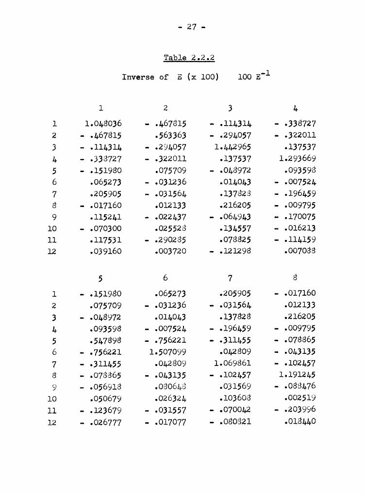
2.2 Preparation of DataThe matrix of sums—of—squares and sums-of—products

within groups E is given in Tgble 2.2.1 andE”l

is

given in Table 2.2.2. The construction of the z variables,

the matrix E, and its inverse E°l were obtained on the

I. B. M. 650 electronic computer by use of the Revised

General Multiple Regression System (06.2.008). The matrix

of estimated correlations R was obtained in the following

manner: Let the (i, j)th element of E be eij , then the

estimated correlation of the ith and jth variable wculd be

aliThus,(2.2.1) R E Dl/YEEE

where Dl/35;; is a diagonal matrix with diagonal elements

- ZA -

Table 2.1.1

Population Means and Variances*

Group I Group II Group III

21 38, 10 29, 10 20, 10

22 60, 26 L5, 26 30, 26

23 20, 2 15, 2 10, 2

zu 27, 5 21, 5 15, 5

25 37, 37 hä, 37 59; 3726 20, 10 26, 10 32, 10

27 15; 5 19, 5 23, 528 16, 2 15, 2 la, 2

29 12, 2 10, 2 ll, 2Zlo 33; 17 25, 17 29, 17211 21, 3 20, 3 ‘ 19, 3212 52, 38 L2, 38 50, 38

*An entry in the table of u, 62 means that the

variable is distributed normal with mean u andvariance oz .

- 25 -

Table 2.2.1

Matrix E

l 2 3 A1 783.2361 1153.8681 211.1520 170.98152 1153-8681 1987-1912 107-7200 771-99153 211.1520 107.7200 161.2637 119.11181 170-9815 771.9915 l19•l118 389•9l155 216.7007 227.3985 6.0731 87.08616 106-3891 117-1361 2-6563 13-32617 19.2612 23.9381 - 21.3131 23.29768 19.8597 20.7101 - 18.6569 13.71819 - 31.2610 — 38.0216 — 10.3188 5.7388

10 - 97.9325 - 152.7116 - 16.5333 - 20.288811 213.8801 116.7521 71.2785 169.619312 - 81.7115 — 113.3096 7.3703 12.5116

5 6 7 8

1 216.7007 106.3891 19.2618 19.85972 227.3985 117.1361 23.9381 20.71013 6.0731 2.6563 — 21.3131 — 18.65691 87.0861 13.3281 23.2976 13.71815 2921.1632 1165.9236 881.6001 106.01686 1165.9236 802.0511 110.1736 206.13557 881.6001 110.1736 372.1585 136.21628 106.0168 206.1355 136.2162 118.19189 7-2575 · 1.1125 10.1521 7.6397

10 - 253.9752 - 112.1166 - 62.2690 — 39.623611 191.6827 251.1353 153.8361 83.106112 173.6293 68.0215 93.9127 17.6623

- 36 -

Table 2.2.1 (Cont.)

9 10 11 121 — 31.2640 - 97.9325 243.8801 — 81.71152 - 38.0216 — 152.7416 416.7521 ~ 113.30963 10.3488 — 16.5333 71.2785 7.37034 5.7388 ~ 20.2888 169.6193 12.54465 7•2575 — 253•9752 494.6827 173.68936 - 4.1125 - 142.1466 251.1353 68.02157 10.4524 — 62.2690 153.8364 93.94878 7.6397 - 39.6836 83.1061 17.66239 155.3080 250.3869 — 2.8052 386.2087

10 250.3869 1078.1841 — 50.6908 1484.640711 — 2.8052 — 50.6908 240.5619 50.989312 386.2087 1484.6407 50.9893 2415.9008

- 27 -

Table 2.2.2

Inverse of E (x 100) 100 E°l

1 2 3 41 1.048036 — .467815 · .114314 — .3387272 — .467815 .563363 — .294057 — .3220113 — .1143lh - .294057 l•4h29Ö5 -1375374 · .338727 - .322011 .137537 1.2936695 — .151980 .075709 · •048972 .0935986 .065273 - .031236 .014043 — .0075247 .205905 - .031504 •l37828 - .19Öh598 — .017160 .012133 .216205 · .0097959 .115241 — .022437 — .064943 · .170075

10 · -070300 -025528 -134557 — -01621311 .117531 - .290285 -078825 - .11415912 .039160 .003720 — .121298 .007088

5 6 7 8

1 — .151980 .065273 .205905 » .0171602 .075709 · .031236 — .031564 .0121333 — .048972 .014043 .137828 .2162054 -093598 • .007524 — •l9Öh59 - .0097955 .547898 - .756221 · .311455 — .0788656 — .756221 1.507099 .042809 - .043135

7 — •3ll455 .042809 1.069861 — .1024578 — .078865 — .043135 - .102457 1.1912459 - .056918 .080648 .031569 - .088476

10 .050679 .026324 .103608 .00251911 · .123679 — .031557 — .070042 — -20399612 — .026777 — .017077 — .080821 .018440

- 28 -

Table 2.2.2 (cout.)

9 10 11 12

1 .115241 - .070300 .117531 .0391602 - .022437 .025528 — .290285 .0037203 - .064943 .134557 .078825 - .1212984 - .170075 '

- .016213 - .114159 .0070885 — .056918 .050679 - .123679 - .0267776 .080648 .026324 — .031557 — .0170777 .031569 .103608 — .070042 — .0808218 — .088476 .002519 — .203996 .0184409 1.12953h — .08199h .088817 — .127282

10 — .08199h .880481 .098820 - .54000011 .088817 .098820 1.301669 - .09766512 · .127282 - .540000 — .097665 .402893

- 29 -

l/VSE; . The calculation of R was accomplished by theInterpretive Matrix Operations (05.2.002) on the I. B. M. 650.The matrix R is given in Table 2.2.}, and R°l inTable 2.2.g.

2.3 Factor Analysis

The Factor Analysis performed in this study was done

in order to determine the structure of this sampling problem.The rotation to the Simple Structure will enable us todivide the variables into representative sets. Once thisstructure has been determined, the discriminant function foreach set may be calculated and in turn one may find thecorrelations of the observable variables versus the dis-criminant functicn (artificial variable). These correlationswill then be the basis for ordering the observable variables.

The complete Factor Analysis was computed on the I. B. M.650 by Factor Analysis programs (6.6.021) of [3].

Table 2.}.1 represents an improved centroid solutionwhich was used as input for the maximum—likelihood iterationsand for the purpose of making a preliminary decision regard—

ing the number of factors. This preliminary test is given

in Table 2.}.2.

- 30 -

Table 2.2.3

Matrix of Correlations R

1 2 3 4

1 1.000000 .924819 .686982 .8522612 .924819 1.000000 .720179 .8769543 .686982 .720179 1.000000 .5947794 . 852261 . 876954 . 594779 1 .0000005 .143190 .094327 .008844 .0815576 .134230 .093014 .007386 .0774797 .035668 .027823 — .087087 .0611358 .058293 .038161 — .120687 .0570709 — .089640 - .068435 - .065392 .023321

10 — .106570 — .104342 — .039650 ~ .03129111 .561845 .602714 .361890 .55383112 - .059401 - .051612 .011808 .012925

5 6 7 8

1 .143190 .134230 .035668 .0582932 .094327 .093014 .027823 .0381613 .008844 .007386 — .087087 - .1206874 .081557 .077479 .061135 .0570705 1.000000 .957215 .844757 .6167816 .957215 1.000000 .805898 .5979927 .844757 .805898 1.000000 .5799278 .616781 .597992 .579927 1.0000009 .010769 — .011652 .043459 .050358

10 — .143035 — .152858 — .098262 - .09927811 .589811 .571733 .513933 .44015712 .065348 .048866 .099040 .029519

.. jl ...

Table 2.2.ß (Cent.)

9 10 11 121 - .089640 — .106570 .561845 — .0594012 — .068435 — .104342 .602714 — .0516123 — .065392 - .039650 .361890 .0118084 .023321 — .031291 •553831 .0129255 .010769 — .143035 .589811 .0653486 - .011652 - .152858 .571733 .0488667 .043459 - .098262 .513933 .0990408 .050358 • .099278 .440157 .0295199 1.000000 .611883 — .014513 .630501

10 .611883 1.000000 — .099533 .91988911 — .014513 • .099533 1.000000 .06688512 .630501 .919889 .066885 1.000000

Debarminamt of R = .00000336e9622

- 32 -

Table 2.2.4

Mazrix R'l

1 2 3 41 8.208512 — 5.836711 - .406284 · 1.8718662 - 5.836711 11.196745 - 1.664739 - 2.8347413 — .406284 - 1.664739 2.326971 .3448734 - 1.871866 - 2.834741 .344873 5.0442185 — 2.299995 1.825134 - .335983 .9994176 .517384 - .394414 .050189 - .0420637 1.112115 — .271547 .337777 - .7486968 - .058538 .065904 .334230 - .0235399 .401938 - .124661 .102772 · .418528

10 — .645977 .373719 .561058 — .10517911 .510165 — 2.007187 .155259 - .34963812 .538625 .081499 - .757098 .068846

5 6 7 8

1 — 2.299995 .517384 1.112115 - .0585382 1.825134 — .394414 - .271547 .0659043 - -335983 .050189 -337777 -3342304 -999417 · -042063 — -748696 - .0235395 16.020433 -11.580732 — 3.250564 — .5175886 —11.580732 12.087967 .234184 - .1503517 — 3-250564 -234184 3-984793 — -2407458 — .517588 — .150351 - .240745 167653699 - -383667 -284755 -075933 — -134266

10 .899803 .244841 .656583 .01005111 · 1.037676 — .138248 — .209648 — .38515112 — .711569 — .237859 - .766676 .110353

..33..

Table 2.2.4 (Cout.)

9 10 11 121 .401938 - .645977 .510165 .5386252 — .124661 .373719 — 2.007187 .0814993 .102772 .561058 .155259 - .7570984 — .418528 — .105179 — .349638 .0688465 ~ .383667 .899803 — 1.037676 — .7115696 .284755 .244841 - .138248 - .2378597 .075933 .656583 - .209648 - .7666768 — .134266 .010051 - .385151 .1103539 1-754263 — -335519 -171683 - -779670

10 — .335519 9.493215 .503281 - 8-71525911 -171683 -503281 3.131309 — -74455312 - -779670 - 8.715259 · -744553 9-733502

- 34 -

Table 2.3.1

Improved Centroid Solution for F

l 2 3 4 5l ·Ö39272 •353586 .617691 -.031142 -.0192892 .648319 .344169 .651531 .062182 .0659023 .417864 .200558 .565298 -.177402 .0263784 .630414 .242303 .581188 .203596 -.1090265 .668936 .286984 -.644712 -.178239 -.0888796 .638772 .295459 -.624540 -.192338 -.0550627 .564108 .2003hh -.626736 .016578 -.0246718 .434837 .176577 -.493017 .199836 .0236769 .258480 -.628913 -.044823 .151889 -.136842

10 .245689 -.911991 .077838 -.057242 .03609111 .765070 .316069 -.026707 .096924 .18098612 .432299 -.875119 -.033021 -.094667 .100788

Table 2.3.2

Tests of Partial Independence (see (1.3.2))

(Preliminary)

Independence 1034.89 < 10°6

1 Factor 977.05 <l0”6

2 Factors 698.43 <, l0°6

3 Factors 114.34 .0001

4 Factors 62.56 .60

5 Factors 49.80 .93

„ 35 -

Clearly, two factors are insufficient to explain theobserved dependence. The decrease in the X2-value is rathermarked but, according to the preliminary test, three factors

are not sufficient. Four factors are clearly sufficient.It must be noted, however, that the X2—value will be smaller,

and hence the associated probability larger, once the

maximum-likelihood solution is available. Following thepreliminary decision, 4 factors were used for the iterationinto a maximum—likelihood solution. The procedure wasstopped when all communalities agreed to four places. This

required 35 iterations. The test for partial independence

was repeated yielding, for 4 factors, a x2 of 13.105

(66 d.f.) corresponding to a normal curve equivalent of

6.33, which denotes an extremely high probability ( > l—1O”9).

There may thus be a possibility that three factors would bequite sufficient. The maximum-likelihood solution for threefactors was also established (after 45 iterations starting

from centroid) and, finally, also that for 2 factors (after10 iterations starting from the principa1—axes form of the

three-factor solution). The X2-values for 3 and 2 factors,respectively, were X2 = 28.702 (66 d.f.), normal curve

equivalent 3.87, corresponding to a probability of .99995 5x2 = 247.58 (66 d.f.), normal curve equivalent -10.81,

corresponding to a probability less than 10'2O. Hence thefinal indicating sequence (see [2]) is, for the probability

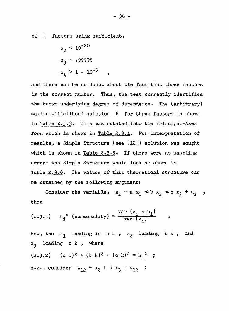
- 36 -

of k factors being sufficient,

-20dz < 10@3

Ä l -l0”9 ,

and there can be no doubt about the fact that three factorsis the correct number. Thus, the test correctly identifiesthe known underlying degree of dependence. The (arbitrary)maximum-likelihood solution F for three factors is shownin Table 2.Q.}. This was rotated into the Principal-Axesform which is shown in Table 2.}.g. For interpretation ofresults, a Simple Structure (see [12]) solution was sought

which is shown in Table 2.}.j. If there were no samplingerrors the Simple Structure would look as shown inTable 2.}.6. The values of this theoretical structure canbe obtained by the following argument:

Consider the variable, zi = a xl eéb x2 +¤c X3 + ui ,then

var (zi — ui)(2.3.1) hiz (communality)i

Now, the xl loading is a k , x2 loading b k , and

x3 loading c k , where

(2-3-2) (a 102 +— tb k>= + (c 1.:)*2 = biz sß e.g., consider 212 = x2 + 6 x3 + ulz 2

- 37 -

TableMaximum-Likelihood Solution

F Matrix after 15 Iterations (3 Factor)

l 2 3

1 -635837 -353673 •59h32h2 •Öh08hh ·3h76lh -6657593 •h50229 -195895 ·5387h61 -603770 -255958 •ÖO5lÖh5 .681370 .287370 -.6636686 -653979 •2922b3 —•6h3h77

7 .565200 -19h770 -.607817

8 -110116 .1833hl ·•h337h79 -210975 --596202 -.021891

10 .251358 --919182 -079711

ll .751218 -301190 -012109

12 .131715 —-883180 --035051

- 38 -

Table 2.•ä•&

Principal Axes (3 Factor)

1 II III 112

1 .762127 .515839 -.057958 .8825912 .768311 .615196 -.071623 .9717523 .521373 .198711 -.103811 .531328

1 .688831 .552083 -.130310 .796276

5 .691125 -.710350 .021893 .9873026 .673851 -.686851 .036257 .9271577 .551983 -.619625 -.012881 .7268618 .120767 -.160613 .026622 .389916

9 -.070372 -.101167 -.631581 .11111510 -.201377 -.026255 -.931606 .915917ll .806310 -.018369 -.085010 .65970712 -.035835 -.157335 -.971973 .970769

..39..

Table 2.3.5

Simple Structure 3 Factors

VAr· A A A biz ääläääiää1 .927 .062 -.0Al .8826 A

2 .981 .011 -.030 .97L8 A

3 .729 -.059 .025 .5313 A

A .890 .005 .036 .7963 A

5 .019 .989 -.008 .9873 B

6 .017 .959 -.023 .9272 B

7 -.037 .8h9 .031 .7269 B

8 -.011 .62h -.016 .3899 B

9 -.017 -.010 .6Ll .L1hl C

10 -.0lA -.17A .9h5 .9159 C

ll .563 .5Lh .03h .6597 A and B

12 .026 .031 .982 .9708 C

.. [FO ..

Table 2 • ä• 6

Expected Simple Structure (3 Factors)

xl x2 X3 hiz

1 .9L9 .000 .000 .900

2 .981 .000 .000 .962

3 .707 .000 .000 .500

L .89A .000 .000 .800

5 .000 .986 .000 .973

6 .000 .9h9 .000 .900

7 .000 .89h .000 .800

8 .000 .707 .000 .500

9 .000 .000 .707 .500

10 .000 .000 .970 .9hl

12 .000 .162 .973 .97h

- hl -

hlzg = sv/38 „kg + 36 kg ¤ 37/38 , 6r kg = 1/38 ,

k = 1/#38 = .162 .

Hence the xl loading is 0, x2 loading .162 and x3

loading .973 (6 x 1.62).A comparison of Table 2.}.Q (observed Simple Structure)

with Table 2.}.6 (theoretical Simple Structure based upon

the population parameters) shows the good agreement of all

values, and hence demonstrates the usefulness of the method

of analysis, even for a comparatively small sample.

Incidentally, if we had taken the overfactored study

(A factors) as a starting point, the same result would have

shown in the Simple Structure. Table 2.ß.Z shows the Simple

Structure formed from the four factor solution. A fourth

overdetermined plane could not be found.

As expected the Simple Structure produced three

representative sets and they are as follows:

Set I — Variables l, 2, 3, A, and ll

Set II — Variables 5, 6, 7, 8, and ll

Set III · Variables 9, 10, and 12 .

2.A Discriminatory Analysis

The discriminant function g is given by the expression

(2•A•l) E—l H g ¤ Reg ,

- A2 -

Table 2.}.]

Simple Structure L Factors

AAA· A A A ääliäfiäiää1 .91A .066 -.037 A2 .970 .007 -.032 A

3 .695 -.0AO .036 A

L .902 —.008 .029 A5 .00u .992 .000 B

6 .005 .952 -.016 B

7 -.023 .828 .025 B8 .017 .596 -.026 B9 -.007 -.017 .637 C

10 -.017 -.172 .9h7 C

11 .577 .522 .026 A and B12 .022 .029 .978 c

- #3 -

and the solution for gg is the eigenvecter associated with

the largest characteristic root of E°lH, where E°l is the

matrix given in Table 2.2.2 and H is the matrix for the

hypothesis of no group differenees. Hence the elements must

be sums—ef—squares and products "between groups", er3....„ ·-(1) ===(1) ·—(;1) ·-(3)(2.u.2) hij rilnr(xr — x )(xT — x ) ,

where agp) is the mean of the p'th variable in the r'th

group, and §(p) is the mean ef the p'th variable over all

3 groups.New, for ease of calculatien let B B* = H, where the

(i, r)'th element of B is , and nris the size ef group r . Thus the matrix B in Set I

mentioned above would be:

(gäl) __ gw), G-{il) __ gw), (ggl) __ gw.),6;,2) _ gw), (géz) _ gw), G-(,,2) _ gw),

__ =;w), (géß) _ gw), (géß) __ gw),,;,1+) __ gta), G-;.) _ ggu.), (3;;:.) _ gu.),

(gäll) __ g(l1), (géii) _ g(ll), (-5-cgll) __ g(11),

using variables l, 2, 3, A, ll. These calculations were

further eased by utilizing the following relations:

- gg -

_ T (1) _Eil) =·-£gü- where TP(l) is Th? total of the i'th. ivariable in group r ; =;)l) = ggü- where G(i) is

the total of the i'th variable over all three groups.

Now, by Eguation (2.g.l),

(2.4.3) E°l B B' g = N_g and

(2.1,.1.) B• B"l B [B• gl = A.[B· g] .Now let B*_g =_g , hence

(2.4.5) B' E°l B g = k_g .

Ne find the largest characteristie root of the small

Symmetrie matrix B7 E°l B and the eigenveetor associated

with the root is g . (Note that E°l H would be non-

symmetric, 12 x 12, whereas B' E°l B is Symmetrie,

3 x 3J Then from Eguation (2.4.j),

(2.1,.6) B"l B B• B"l B E =—— A B"l B _g_ or

(2.1,.7) B"l B [B°l B gl —-= A. [B‘l B gl , hence(2.1,.2%) g = B°l B E

and the desired diseriminant function is solved.

This procedure was followed in obtaining the discriminant

function for each of the three sets derived from the Simple

Structure and also for the Set of all twelve variables taken

together. The task was perfermed as followsz

(a) The matrix B computed

- 25 „

(b) The matrix E°l B and B' E°l B computed usingthe Matrix Interpreter

(c) Characteristic roots and associated eigenvectors

of B' E°l B were obtained(d) The largest characteristic root and associated

eigenvector E was chosen(e) Using E and

E”lB from above E°l B g was

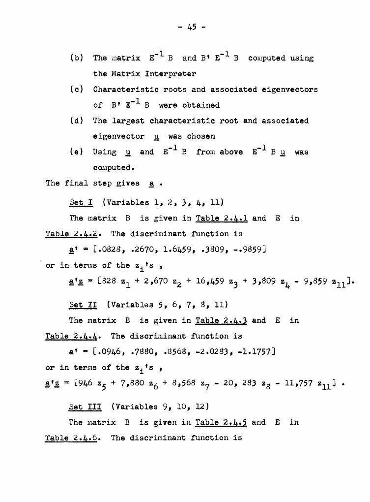
computed.The final step gives gr.

Set I (Variables 1, 2, 3, 4, ll)The matrix B is given in Table 2.g.l and E in

Table 2.g.2. The discriminant function isg' = [.0828, .2670, l.6A59, .3809, -.9859]

or in terms cf the 2i's ,g{g “ [828 Zl + 2,670 Z2 I l9•h59 23 + 3,809 zu - 9,859 211].

Set II (Variables 5, 6, 7, 8, 11)

The matrix B is given in Table 2.g.Q and E in

Table 2.g.g. The discriminant function is

a' ¤ [.09h6, .7880, .8568, -2.0283, -1.1757]or in terms of the 2i*s ,Q'2 = [9h6 25 + 7,880 26 + 8,568 27 — 20, 283 28 — ll.757 Zll] .

Set III (Variables 9, 10, 12)

The matrix B is given in Table 2.g.j and E inTable 2.g.6. The discriminant function is

- A6 -

Table 2.4.1

Matrix B Set I (Variables 1, 2, 3, 4, 11)

1 2 3

1 49.8840 1.2101 -51.0941

2 81.3360 4.1348 -85.4709

3 25.6413 2.4560 -28.0973

4 31.89hB 2.7882 -34.6825

11 4.5844 1.4907 - 6.0750

Table 2.4.2

Matrix E Set I (Variables 1, 2, 3, 4, 11)

1 2 3 4 11

1 783.2361 1153.8684 244.1520 470.9815 243.8801

2 1153.8684 1987.4942 407.7200 771.9945 416.7521

3 244.1520 407.7200 161.2637 149.1448 71.2785

1+ 1+70 •9815 771.991+5 l1+9·l1+1+8 389• 911+5 169 .619311 243.8801 416.7521 71.2785 169.6193 240.5619

- 47 -

Table 2.4.}

Matrix B Set II (Variables 5, 6, 7, 8, ll)

1 2 3

5 -57.6623 4.8951 52.7672

6 -31.9302 2.4607 29.4696

7 -21.7481 2.2249 19.5232

8 5-5677 -2918 ·— 5-8595ll 4.5844 1.4907 - 6.0750

Table 2.4.4

Matrix E Set II (Variables 5, 6, 7, 8, ll)

S 6 7 8 115 2924-1632 1465.9236 881.6001 406.0168 494.6827

6 1465.9236 802.0511 440.4736 206.1355 251.1353

7 881.6001 440.h736 372.4585 136.2462 153.8364

8 406.0168 206.1355 136.2462 148.1918 83.1061

11 h9h.6827 251.1353 153.8364 83.1061 240.5619

- 43 -

Table 2.4.5

Matrix B Set III (Variables 9, 10, 12)

1 2 3

9 4.1024 - 6.1467 2.044310 15.4846 -18.4680 2.9834

12 13.0248 -29.1103 16.0855

Table 2.4.6

Matrix E Set III (Variablee 9, 10, 12)

9 10 12

9 155.3080 250.3869 386.2087

10 250.3869 1078.1841 1484.640712 386.2087 1484.6407 2415.9008

- AQ -

ä' “ K·lÖ7l. •5778; --3398]or in terms of the 2i*s ,

afg = K1,67l 29 + 5,778 210 — 3,398 212] .

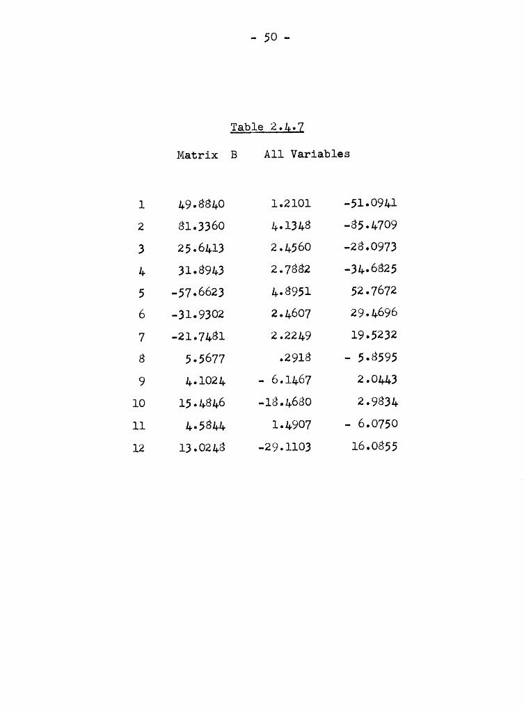
Set of all variables

The matrix B is given in Table 2.4.] and E inTable 2.1.1. The discriminant function is

a' = [-.2547, -.1163, -2.1608, -.1431, .1376, .6685,.1992, -2.6915, -.1175, -.3834, .5770, .2301]

andg{g ¤ K- 2547 21 - 1163 22 - 21,608 23 - 1431 zu

#-1376 25 + 6685 26 #-1992 27 - 26,915 28

- 1175 29 — 3834 210 + 5770 zll + 2301 212] .

2.5 Ordering

As expressed above we may regard the discriminant func-tion as an artificial variable which is a linear combinationof the observable variables. 0ne may interpret the relativecontribution of each observable variable to this artificialvariable by computing the correlations of the artificialvariable versus the observable ones. The correlation riof the artificial variable versus an observable one wasevaluated using the relation (see Eguation (1.2.8))

(2.5.1) ri = (g' E)i/{§*“E_gfeii

- 50 -

Table 2.4.7

Matrix B A11 Variables

1 49.8840 1.2101 -51.0941

2 81.3360 4.1348 -85.4709

3 25.6413 2.4560 -28.0973

4 31.89hB 2.7882 -34.6825

5 -57.6623 4.8951 52.7672

6 -31.9302 2.4607 29.4696

7 -21.7481 2.2249 19.5232

8 5•5677 •29l8 — 5-85959 4.1024 - 6.1467 2.0443

10 15.4846 —l8•4Ö3O 2.9834

11 4.5844 1.4907 - 6.0750

12 13.0248 -29.1103 16.0855

- 51 -

where (af E), represents the i*th element of the rowvector g' E , and ei, is the (i, i) diagonal elementof the matrix E presented in Tables 2.1.1, 2.A.2, 2.A.A,

or 2.A.6. Now in vector form g' ¤ [rl rz ... rp], hence

(2.5.2) _;·=-—-—-?-·-—- gs ml/1,,-. .{Q' E a ii

This g' was evaluated for each of the three sets andthe set of all observable variables taken together. The

results are as follows:

Set I (variables 1, 2, 3, A, ll)

1 2 3 A 11g' = [.7669, .7962, .9022, .7186, .1A78]

Set II (variables 5, 6, 7, 8, ll)5 6 7 8 ll

g' = [.A771, .5065, .A999, -.2186, -.1592]

Set III (variables 9, 10, 12)9 10 12

g' = [.3929, .6069, .2566]

Set of all variables (1, 2, 3, ..., 12)

1 2 3 L 5 6g' = [.5888, .6109, .6913, •5507, —•3327, -·3533,

7 8 9 10 ll 12-.3A83, .1533, .02A6, .0595, .1126, -.1295] .

- 52 -

The order will then be determined by the descending

order of magnitude or modulus, thus§gg_I : order — (3, 2, 1, 4, ll)

Set II : order — (6, 7, 5, 8, ll)

Set III : order - (10, 9, 12)

Set of all variables : order · (3, 2, 1, 4, 6, 7,

5, 8, 12, 11, 10, 9)

2.6 SelectionClearly, from the construction of the variables, 23

was expected to have the highest discriminating power (the

standardized difference between two groups there was

(20 - 15)/#2 + 3.5 , and this vaiueis larger than that for any other variable. On the other

hand if, e.g., only three variables were to be selected for

future purposes, the overall discriminant function would

tell us to use 3, 2, 1 which as the factorial structureshows, are purely representative of one factor only (see

discussion on anthropological and physiological measurements

in the introduction). Making use of the fact that the

twelve variables fall into three sets, our representative

choice would be 3, 6, 10 . These are, in fact, the best

discriminators in each set.

- 53 -

Chapter III: DEMONSTRATION STUDY 2

3.1 Description of Data

The data used in this study were taken from T. G.

Thurstone's study given in [13]. The experimental units in

this case were mentally retarded children from both public

and special schools. These children were not institution—

alized, but are in the lower range ef the normal pepulation.

Many types of test were taken by these children and the

findings are presented in [13]. we have chosen 12 of these

tests as eur ebservable variables. They are as fellewsz

21 = Binet Mental Age22 = "Primary Mental Abilities Test" Mental Age

23 = Achievement Paragraph Meaning

zh ¤ Achievement Werd Meaning

25 ¤ Achievement Spelling26 ¤ Achievement Arithmetic Reasening27 = Achievement Arithmetic Computatien

28 = Gain Paragraph Meaning

29 = Gain Word Meaning

Zlo = Gain Spelling

211 = Gain Arithmetic Reasening212 = Gain Arithmetic Cemputatien .

Variables zl and 22 are measnred in months and variables23, zh, ..., 212 are measured in grade equivalents, i.e., a

- 5h -

response of 2.0 would indicate performance at the second

grade level. The children were placed in three age groups:

young (10 years ll months and younger)

middle (ll years to 12 years ll months)old (13 years and older) .

Previous analysis of these data showed a significant

interaction between school types and age groups; the older

group performed much better in public schools than either the

young or middle group. For this reason we have made three

separate studies to find the discriminating variables between

public and special schools; one study for each age group.

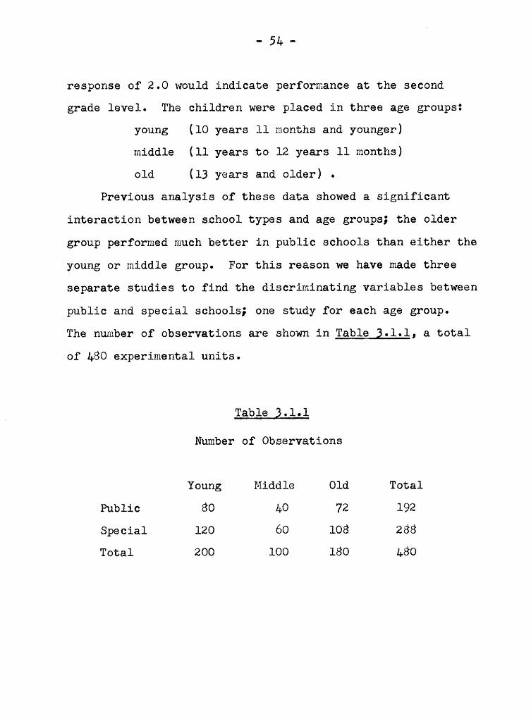
The number of observations are shown in Table @.1.1, a total

of A80 experimental units.

I Table @.1.1Number of Observations

Young Middle Old TotalPublic 80 40 72 192Special 120 60 108 288Total 200 100 180 480

- 55 -

The matrix of corrected sums-of—squares and products pooled

over the six groups is presented in Table @.1.2 and is denotedas the matrix E . The matrix of correlations R is presentedin Table @.1.}. These matrices were obtained by the same

methods as presented in Chapter II.

3.2 Factor AnalysisThe Factor Analysis performed in this study was done in

the same way as in Chapter II. An improved centroid solution

for F was obtained and iterated into the maximum-likelihoodestimate of F (25 iterations) with five factors. The final

decision was five factors since e5 was approximately .92

(normal curve equivalent of 1.41) indicating a good plausi-

bility of five factors. The maximum—1ikelihood solution for

F after 25 iterations is presented in Table @.2.1.

Once F was obtained and the decision of the number of

factors made, the "Principal Axes" (standard for comparison

as indicated in Chapter I) was obtained by rotation, and is

presented in Table @.2.2; the communalities are also given

there. The "Simple Structure" was then obtained by rotation

for the purpose of identifying the variables belonging to

common-factor sets. The Simple Structure is presented in

Table @.2.@. The five sets found were: A, which contains

intelligence measures (variables l, 2, 6, 7); B, which con-

tains achievement measures (variables 3, 4, 5, 6, 7);

..56..

Table 3.1.2

Matrix E

l 2 3 Ä1 59450.00 49485.00 2088.80 2091.402 Ä9485.00 92416.00 2944.20 2864.00

3 2088.80 2944.20 434.90 373.884 2091.40 2864.00 373.88 417.795 2275.10 3088.60 407.08 421.276 2952.40 3786.80 313.93 299.427 3229.30 4234.10 281.46 273.108 138.40 62.10 - 29.49 23.06

9 127.30 49.90 24.50 — 6.6010 104.40 357.50 31.65 37.2511 210.20 42.30 32.08 29.6912 55.00 214.30 20.07 14.40

5 6 7 8

1 2275.10 2952.40 3229.30 138.402 3088.6 3786.80 4234.10 62.10

3 407.08 313.93 281.46 — 29.494 421.27 299.42 273.10 23.06

5 665.19 367.64 350.28 40.346 367-64 414-96 373.12 24-757 350.28 373.12 554.53 16.918 40.34 24.75 16.91 141.259 Ä2-30 26.40 33-Ä? 41-48

10 22.90 31.07 29.20 23.5311 47.50 - 5.70 39.91 18.5312 22.09 21.60 16.51 8.95

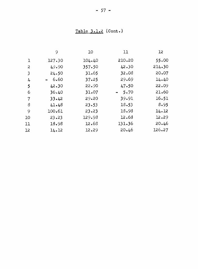
- 57 „

Table §.1.2 (Comt.)

9 10 11 12

1 127.30 101.10 210.20 55.002 49.90 357·5O 12.30 211•3O3 21.50 31.65 32.08 20.071 - 6.60 37.25 29.69 11.105 12.30 22.90 17.50 22.096 36.10 31.07 — 5.70 21.607 33.12 29.20 39.91 16.518 11.18 23.53 18.53 8.959 100.61 23.23 18.98 11.12

10 23.23 129.98 12.68 12.2911 18.98 12.68 131.36 20.1612 11.12 12.29 20.16 126.27

- 53 -

Table 3.1.3

Matrix of Correlations R

l 2 3 11 1.000000 .667612 .110796 .1196152 .667612 1.000000 .161107 .1609153 .110796 .161107 1.000000 .8771191 .119615 .160915 .877119 1.0000005 -361786 .393927 -756851 .7991116 .591121 .611199 .738981 .7191167 ·562132 -591159 -573138 .5673888 .017760 .017188 — .118983 .0919269 .052051 .016365 .117125 — .032192

10 .037557 .103119 .133119 .15981911 .075219 .012110 .131217 .12673612 .020071 .062733 .085615 .062695

5 6 7 81 .361786 .591121 -562132 -0177602 .393927 .611199 .591159 .0171883 -756851 -738981 -573138 — .1189831 .799111 .719116 .567388 .0919265 1.000000 .699756 .576710 .1316016 .699756 1.000000 .777327 .1022307 .576710 .777827 1.000000 .0601218 .131601 .102230 .060121 1.0000009 .163511 .178117 .111189 .317956

10 .077880 .133783 .108763 .17365611 .160690 - .021111 .117873 .13603512 .076221 .091363 - .062393 .067016

- 59 -

Table 3.1.3 (Comt.)

9 10 11 12

1 .052051 .037557 .075219 .0200742 .016365 .103149 .012140 .0627333 .117125 .133119 .134217 .085645

4 — .032192 .159849 .126736 .0626955 .163511 .077880 .160690 .0762216 .178147 .133783 — .024414 .09h3637 .141489 .108763 .147873 — .0623938 .347956 .173656 .136035 .0670169 1.000000 .203138 .165099 .125275

10 .203138 1.000000 .097040 .09593211 .165099 .097040 1.000000 .15886312 .125275 .095932 .158863 1.000000

Determinant of R = .001001523

- 60 -

Table 3.2.1

Matrix F (Maximum-Likelihood Solution, 25 Iterations)

1 2 3 4 5

1 .628866 .230941 -.321293 .336145 .0433742 .638647 .278587 -.265802 .326764 .015320

3 .809300 .284088 .431709 -.040941 -.258013

4 .809083 .321143 .420957 -.112223 .214127

5 .764734 .137118 .245682 -.186324 .054366

6 .870004 .319699 -.224076 -.278563 -.113919

7 .735920 .233001 -.229531 -.024823 -.041500

8 .248250 -.488106 -.166390 -.204546 .456236

9 .354375 -.696355 -.115519 -.123671 -.282028

10 .224312 -.179844 .039434 -.043212 .062182

11 -185520 —•265430 -180950 .199239 .042936

12 .120990 -.104362 .004798 -.063868 -.050182

- 61 -

Table ä•2•2

Principal Axas

I II III IV V hi?

1 .613 .079 -.160 .027 .188 .6669

2 .668 .129 -.108 .005 .185 .6631

3 .877 .131 .375 -.238 .085 .9903

1 .880 .106 .381 .210 .071 .9931

5 .787 -.081 .263 .073 -.035 .7017

6 -926 -.017 —·lh5 --055 --3hh -99997 .763 -.010 -.239 -.019 -.102 .6509

8 .100 -.625 -.063 .111 -.036 .5775

9 .159 -.755 -.023 -.350 .012 .7187

10 .169 -.233 .055 .010 .018 .0899

11 .106 -.223 .099 -.017 .329 .1791

12 .092 -.137 .032 -.057 -.025 .0321

- 63 -

Table 3.2.3

Simple Structure

A B C D E

1 .693 -.031 .017 .010 .0352 .661 .026 -.025 -.003 -.0273 .011 .753 .006 .065 -.330

4 -.004 .803 -.008 -.306 -.0255 .023 .659 .134 -.069 .0386 .372 .h95 -.021 -.009 -.0347 .458 .271 .030 .017 .0178 .006 .003 .553 .021 .7419 -.002 -.016 •75l .706 .375

10 -.005 .112 .247 .097 .19311 .003 .035 .328 .181 .15912 -.018 .068 .13h .112 .063

Transformation Vectors from F

I II III IV V

.361 .h77 .3h7 .156 .176

.193 .248 -.935 -.653 -.652-.709 .654 .015 -.124 -.277

•57h -.532 .053 .160 -.129.023 .011 .052 -.712 .671

- 63 -

C, which contains gain measures (variables S, 9, 10, ll);

and the other two factors, D and E, of the Simple Structure

are well overdetermined pseudo—factors showing a very high

loading on a verbal gain variable and a negative one on the

corresponding achievement variable. No such inverse relation—

ship was observed in the arithmetic variables. These two

factors, D and E, are probably due to the fact that the

children in the lowest group on the achievement tests had

scores so low in the first administration that they could not

but gain in the second.

3.3 Disgriminatory AnalysisThe discriminant function between school types was

sought for each of the three sets mentioned in Section Q.2,

on each of the three age groups. Also, the overall discrim—

inant function for all twelve variables on each of the three

age groups was determined.

As presented in the previous chapters, the discriminant

vector g is the eigenvector associated with the largest

characteristic root of E°l H , or

(3.3.1)E_l

H g = R_g .

Now, in this case,

2 .. „ ... „„(3•3•2) H == iäl ni (yi ·— y)(yg_ ·- y')

where il is the mean vector for public schools, and E2

- 6h -

the mean vector for special schools. This reduces to theform

(333) -"‘><"‘·-"‘·>·• Z2 •and hence

( ) E°lH==—-L--HH2 E°l(” ”)(°' °°')3·3·¢+ ,,1-...,12 11-12 xl -12 ·We shall denbbe (jl - iz) by Q and (§l•

- §2·) by §•,

hence

-1 _„ **1**2 „—1--(3-3-5) E H H g_g_• ,

Since ch (A B) = ch (B A) , the characteristic root ofE°l H is the same as the characteristic root of

**1 **2 - .-1- .H——;;—— Q' E Q , which is a scaler quantity, hence1 **2I1 Y1,(3_3_6) ;„_„„.....l....§... Ev E"]-;**1+**2

the only non-zero characteristic root of E°l H. Now by

pre-multiplying Eguation (}.}.6) by E°l Q we get

I1 I1l 2 -1 „-l — Q -1 ·(3-3-7) ·5i····;_····;1·2· E QQ' E Q LE Q , A

OT

(3.3.8) E"lH (E"*' QT) =·=7-(E°l li;)-

Hence,(3-3-9) _a_==E"l_°{

-

- 65 -

This vector g , which can, of course, be multiplied by any

arbitrary constant, is equivalent to the discriminant func-

tion for two groups as given by R. A. Fisher (see [7]).

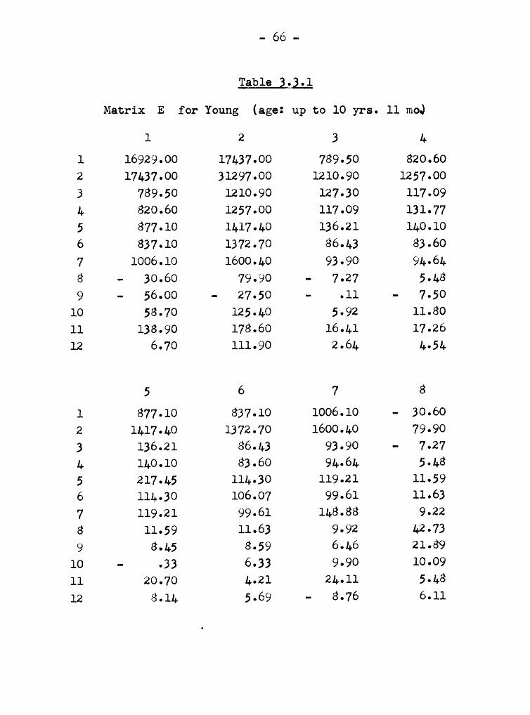
The matrix E for the young group is presented in

Table }.3.1, for the middle group in Table 3.3.2, and the

old group in Table 3.}.3. The mean column vectors for both

public and special schools on all three age groups are shown

in Table 3.}.A, and the difference vectors, E , are shown

in Table 3.3.5.The discriminant functions gfg , are as followe:

(variables 21 and 22 in months, variables 23, 2h,..., 212in grade (year) equivalents. The values of the g's were

multiplied, in each case, by a convenient power of 10).

YoungSet I (variables 1, 2, 6, 7):

gf; = 3.32 21 22 - 50.30 26 27

Set II (variables 3, A, 5, 6, 7):

Z3 •• •3l Zu • •ll Z5 •• •l5 Z6 • •lp2 Z7

Set III (variables 8, 9, 10, ll):

ä{g = 1.50 28 · .88 29 — .90 210 — .67 zll

MiddleSet I :

gfg = .05 21 — .5A 22 · 7A.51 26 + A6.52 27

- 66 -

Table 323;;

Matrix E for Young (age: up to 10 yrs. 11 mo)

1 2 3 4

1 16929.00 17437.00 789.50 820.602 17437.00 31297.00 1210.90 1257.003 789.50 1210.90 127.30 117.094 820.60 1257.00 117.09 131.775 877.10 1417.40 136.21 140.106 837.10 1372.70 86.43 83.607 1006.10 1600.40 93.90 94.648 - 30.60 79.90 - 7.27 5.489 - 56.00 — 27.50 — .11 — 7.50

10 58.70 125.40 5.92 11.8011 138.90 178.60 16.41 17.2612 6.70 111.90 2.64 4.54

5 6 7 81 877.10 837.10 1006.10 — 30.602 1417.40 1372.70 1600.40 79.903 136.21 86.43 93.90 - 7.274 140.10 83.60 94.64 5.48

5 217.45 114.30 119.21 11.596 114.30 106.07 99.61 11.637 119.21 99.61 148.88 9.228 11.59 11.63 9.92 42.739 8.45 8.59 6.46 21.89

10 - .33 6.33 9.90 10.0911 20.70 4.21 24.11 5.4812 8.14 5.69 — 8.76 6.11

..67..

Table 3.}.1 (Cont.)

9 10 11 12

1 — 56.00 58.70 138.90 6.702 — 27.50 125.40 178.60 111.90

3 - .11 5.92 16.41 2.644 - 7.50

6 11.80 17.26 4.545 8.45 · .33 20.70 8.146 8.59 6.33 4.21 5.697 6.46 9.90 24.11 - 8.768 21.89 10.09 5.48 6.11

9 38.85 10.06 6.07 2.8210 10.06 50.18 8.53 7.4711 6.07 8.53 51.26 10.4512 2.82 7.47 10.45 47.32

- 63 -

Table 3.3.2

Matrix E Middle (ages: 11 yr. to 12 yr. 11 mo.)

1 2 3 4

1 113Ä9.00 8922.00 331.40 258.902 8922.00 28755.00 678.30 590.903 331-40 678-30 87-57 75-59Ä 258-90 590-90 75-59 76.935 421.00 648.10 89.60 85.116 548.20 831.90 70.13 60.127 534-50 974.60 67.20 63.738 - 3.90 — 71.10 — 7.08 — 1.299 134.40 69.70 5.15 1.38

10 47.10 202.50 11.11 11.5111 45.90 12.90 10.44 9.6012 38.30 11.00 2.80 .51

5 6 7 8

1 421.00 548.20 584.50 — 3.902 648.10 831.90 974-80 - 71.10

3 89.60 70.13 67.20 — 7.08

4 85.11 60.12 63.73 - 1.29

5 147.26 82.37 65.50 5.416 62.37 95.74 84.63 - 2.387 65.50 84.63 148.19 - 6.598 5.41 - 2.38 - 6.59 23.75

9 12.56 12.05 10.80 9.3210 14.39 16.70 14.14 3.4911 14.55 — 1.02 6.47 4.22

12 5-7Ä 9.03 - 1.31 1.58

- 69 -

Table 3.}.2 (Cent.)

9 10 11 12

1 134.40 47.10 45.90 38.302 69.70 202.50 12.90 11.003 5.15 11.11 10.44 2.80

4 1.38 11.51 9.80 .51

5 l2·56 lh•39 lh•55 5.746 12.05 16.70 · 1.02 9.03

7 10.80 14.14 6.47 ~ 1.318 9.32 3.49 b.22 1.589 17.83 1.60 3.63 3.27

10 1.60 29.96 - 1.18 2.6211 3.63 - 1.18 30.12 2.7912 3.27 2.62 2.79 20.06

- 7Q -

Table @.3.3

Matrix E Old (ages: 13 yr. up)

1 2 3 4

1 31175.00 23126.00 967.90 1011.902 23126.00 32364.00 1055.00 1016.103 967.90 1055.00 220.03 181.204 1011.90 1016.10 181.20 209.095 977.00 1023.10 181.27 196.066 1567.10 1582.20 157.37 153.007 1638.70 1658.90 120.36 114.738 172.90 53.30 — 15.14 18.87

9 48.90 7.70 19.46 - .4810 — 1.40 29.60 14.62 13.9411 25.40 — 149.20 5.23 2.6312 10.00 91.40 14.63 9.35

5 6 7 81 977.00 1567.10 1638.70 172.902 1023.10 1582.20 1658.90 53.303 181.27 157.37 120.36 - 15.144 196.06 153.00 114.73 18.875 300-48 170-97 145-57 23-346 . 170.97 213.15 188.88 15.507 145•57 188.88 257.46 13.588 23-34 15-50 13-58 74-779 21.29 15.76 16.16 10.27

10 8.81 8.04 5.16 9.95ll 12.25 - 8.89 9.33 8.83

12 8.21 6.88 - 6.44 1.26

..'7]_..

Table 3.Q.j (Cent.)

9 10 11 12

1 18.90 - 1.10 25.10 10.002 7.70 29.60 -119.20 91.10

3 19.16 11.62 5.23 11.631 - ·h8 13-91 2.63 9-355 21.29 8.81 12.25 8.216 15.76 8.01 — 8.89 6.887 16.16 5.16 9.33 - 6.118 10.27 9.95 8.83 1.26

9 13-93 11.57 9.28 8.0310 11.57 52.81 5.33 2.20ll 9.28 5.33 19.98 7.2212 8.03 2.20 7.22 58.89

- 72 -

Table 3.3.4*

Means (Public Schools)

Var Young Middle Old

1 76.9500 95.5000 110.05562 76.8250 97.0250 112.28473 1.8975 2-4425 3-32924 1.8688 2.4825 3.25695 1.8638 2.8200 3.6389Ö 1-4850 2-4475 3-51397 1.7762 2.7450 3.85698 .4750 .3025 .29449 .4262 .3925 .2625

10 .5088 .3025 .2806ll .4850 .3375 .283312 .5488 .4225 .3583

Means (Special Schools)

Var Young Middle Old

1 79.2417 93.7000 106.26852 77.1417 93.8333 106.76853 1.2525 1.9050 2.59174 1.4108 1.9667 2.57685 1.4083 2.0367 2.79546 1.3125 2.0850 2.8426

7 l-7325 2-7533 3-48988 .5092 .3850 .34639 -4117 -3717 -3944

10 .4642 .5550 .3231ll .4458 .4550 .442612 .5483 .3683 .3981

*Menta1 Age in months, achievement measures in grade equivalents.

- 73 -

Table 3.}.5

Mean Differences (Public minus Special)

Var Young Middle Old

1 -2.2917 1.8000 3.7870

2 — .3167 3.1917 5.5162

3 •Öl+5O •5375 -7375

4 .4579 .5158 .6801

5 -1.551+ -7833 -81+356 .1725 .3625 .6713

7 .0438 — .0083 .3671

8 - .0322 - .0825 - .0518

9 .0146 .0208 — .1319

10 .0446 - .2525 - .0426

11 .0392 - .1175 - .1592

12 .0004 .0542 - .0398

- 7A -

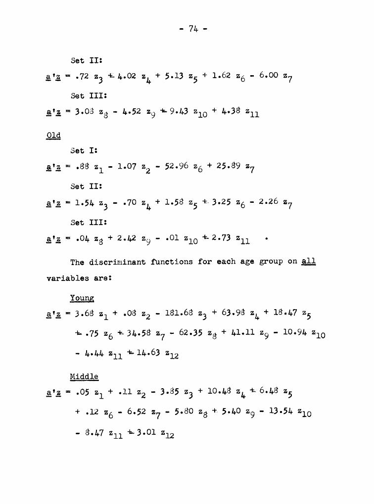
Set II:g'g = .72 23 +-4.02 2h + 5.13 25 + 1.62 26 · 6.00 27

Set III:

gf; = 3.08 28 — 4.52 29 +-9.43 2lO + 4.38 211

QL!Set I:

*' Z7

Set II:

g'; = 1.54 23 - .70 zu + 1.58 25 + 3.25 26 · 2.26 27

Set III:

g{g = .04 28 + 2.42 29 — .01 210 +-2.73 211 .

The discriminant functions for each age group on.g1l

variables are:

Young

g{g = 3.68 21 + .08 22 - 181.68 23 + 63.98 zu + 18.47 25

+—.75 26 +-34.58 27 - 62.35 28 + 41.11 29 — 10.94 210

— 4.44 211 +-14.63 212

Middle

gf; = .05 21 + .11 22 — 3.85 23 + 10.48 2h +-6.48 25

+ .12 26 - 6.52 27 - 5.80 28 + 5.40 29 · 13.54 210

••

- 75 -

01d

= L •' • „- •• • •' •g'g ,36 21 7l za LO 7 23 + 36 3A zh 25 71 25

- 25,86 26 t 20,87 27 - 12,13 23 + 58,15 29 + 3,53 210

*=l9,l2 211 + 10,90 212 ,

3,L OrderingIn order to make a representative selection we must

first order the variables within each "common-factor" set as

to their importance, This is done by ordering them accord-

ing to their absolute correlation with the artificial

variable g{g , These correlations are given by Eguation

{1,2,8}, which states:

P! =¤:7..,,.,,...:!',,.,,•-,,„., äiEig'E g_ ii °

Now, since _a_* E === §' ,

(3.1+.1) 1~• =6—-;-¥—— §• D1/1,é-— .@1* s iiNote that ri is in the form of a standardized mean, Thecorrelations are then as follows:

YoungSet I:

1 2 6 7E, zu [""°l|·lI·! "°°OI+! °l|·2)

- 76 -

Set II:

3 L 5 Ö 72,

zi: •73} °5l}

*39}SetIII:

8 9 10 111*} *= [ ··-LL. -21. -56. -1+8 3

A11 variables:

g' ¤ [ -.19, -.02, .62, .43, .34, .18, .04, -.05, .03, .07,•O6, 000 J

MiddleSet I:

1 2 6 7_;• ¤ ( .31, .35, .69, -.01 JSet II:

3 L 5 6 7

Set III:

8 9 10 11g' = [ -.30, .87, -.85, -.38 ]

All variables:

-.18, .10 ]

- 77 -

$119.Set I:

1 2 6 7g' = [ •&O; •57, .86, .h3 1

Set II:

3 4 5 6 7gv = [ .86, .81, .84, .80, .40 3

Set III:

8 9 10 11g' = [ -.22, -.72, -.21, -.82 ]

A11 variables:

g' = [ .30, .43, .70, .66, .69, .65, .32, -.08, -.28, -.08,

-.32, -.07 3

The orderings then:

1f.9.v1v18set 1 : (1, 6, 7, 2)Set II : (3, 4, 5, 6, 7)

Set III: (10, 11, 8, 9)

111 : (3, 4, 5, 1, 6, 10, ll, 8, 7, 9, 2, 12)

l*i.i§..<1..l.§.sec 1 : (6, 2, 1, 7)Sßb II ! (5. A. 3. Ö, 7)

Set III: (9. 10, 11, 8)

111 : (5, 4, 3, 10, 6, 11, 2, 1 or 8, 12, 7, 9)

- 78 -

.9.l.Qset I : (6, 2, 7, 1)Set II : (3, 5, 4, 6, 7)

· Set III: (ll, 9, 3, 10)

All : (3, 5, 4, 6, 2, 7 or ll, l, 9, 3 or 10, 12) .

3.5 Selection

Now, if we wish to choose the three tests that are

closest to the best discriminator (discriminant function)

between schools, the overall discriminant function would indi-

cate the three achievement tests: Paragraph Meaning, Word

Meaning and Spelling (variables B; he and 5) for all three

age groups. It should be noted that these three variables

all belong to the same common·factor; more specifically, they

are all verbal achievement measures. while these three

doubtlessly show the greatest relative difference between

the public and special school groups, a future study based

on these three alone would completely disregard the gain

measures and intelligence measures originally considered.

A representative selection (one variable from each

factor) would lead to the following choice:

Xgggg; Binet Mental Age, Achievement Paragraph Meaning,

Gain Spelling (variables 1, 3, 10)

Middle; Arithmetic Reasoning, Achievement Spelling,

Gain Word Meaning (variables 6, 5, 9)

- 7Q -

Qlg; Arithmetic Reasoning, Achievement Paragraph Mean-

ing, Gain Arithmetic Reasoning (variables 6, 3, ll).

It must be noted that, for the middle and old group,

Arithmetic Reasoning showed up as the strongest discriminator

on the Intelligence factor (even though the test was denoted

as an ”Achievement" test, and had high loadings on the

achievement factor, too). The achievement factors in this

study are probably more strongly determined by the verbal

tests (see Table }.2.}). The Arithmetic Achievement tests

were as clearly present on the Intelligence as on the

Achievement Factor, on the former, they even represent the

best discriminator•

If additional experiments were to be performed with a

reduced set of variables, and if one were interested in those

variables only which show the strongest relative difference

between the two groups, the three verbal tests found by the

overall discriminant analysis should be chosen. This subset

would not, however, be representative of the whole set of

original variables.The choice of one of the representative sets (depending

on age) would probably not lead to as strong a differentiation

as the former, but all characteristics present in the original

variables would certainly be represented in the reduced set.

- 30 -

BIBLIOGRAPHY

[1] Anderson, T. W. "An Introduction to MultivariateStatistical Analysis", Wiley, New York, 1958.

[2] Bargmann, R. E. "A Study of Independence in Multi-variate Normal Analysis", Inst. of Stat., Univ. ofNorth Carolina, No. 186, 1957.

[3] Bergmann, R. E. and Brown, R. H. "I. B. M. 650 Programsfor Factor Analysis", Virginia Polytechnic Institute,July 1961.

[A] Bargmann, R. E. and Thigpen, C. "Lecture Notes onMethods of Multivariate Analysis", Virginia PolytechnicInstitute, 1961 (being mimeographed).

E61 Brown, R. H. "A Comparison of the Maximum DeterminantSolution in Factor Analysis with Various ApproximateSolutions", M.S. Thesis, Virginia Polytechnic Institute,1960.

[6] Dixon, W. J. and Massey, F. J. "Introduction toStatistical Analysis", McGraw-Hill, New York, 1957.

[7] Fisher, R. A. "The Use of Multiple Measurements inTaxonomic Problems", Ann. Eugen., Vol. 7, 1936.

[8] Heck, D. L. "Charts of Some Upper Percentage Points ofthe Distribution of the Largest Characteristic Root",Ann. Math. Stat., Vol. 31, 1960.

[9] Howe, W. G. "Some Ccntributions to Factor Analysis",Oak Ridge National Laboratories, ORNL 1919 (Physics),l955•

[10] Posten, H. 0. "Pcwer of the Likelihood Ratio Test ofthe General Linear Hypothesis in Multivariate Analysis",Ph.D. Dissertation, Virginia Polytechnic Institute, 1960.

[ll] Roy, S. N. "Some Aspects of Multivariate Analysis",Wiley, 1957.

[12] Thurstone, L. L. "Multiple Factor Analysis", Univ. ofChicago Press, 19AO.

[13] Thurstone, T. G. "An Evaluation cf Educating MentallyHandicapped Children in Special Classes and RegularClasses", Department of Health, Education and Welfare,Contract No. 168 (6A52), 1960.

- 81 -

ACKNOMLEDGEMENTS

ABSTRACT

The purpose of this thesis is a study of procedures of

selecting variables in a multivariate experiment, The linear

discriminant function is used as an artificial variable, its

correlation on the observed variables is evaluated, and the

absolute magnitude of these correlations decide the inclusion

of a given variable in a subset, i

These subsets are obtained by two different methods:

(a) the complete set of variables is subjected to a

discriminant analysis, and the strongest correlates are chosen

as the subset whose members are "closest” to the discriminant

function,(b) the set of variables is broken down into common-

factor subsets, by factor analysis, and the strongest

representative variates in each subset are selected as the

"representative" set of variables, which are thus representative

of all characteristics of the original variables, This type

of "representative” selection is the proposal and it represents

the major portion of the thesis,

Chapter I is a theoretical exposition containing the back-

ground and formulation needed, Chapter II presents an explicit

demonstration study in which the structure is known, Compu-

tational details are explained and comparisons are made between

the known structure and the structure obtained by the sampling

data. Chapter III represents the analysis of a study of data

from an educational experiment on retarded children•