I ,,,, .j ,,3, ' - NASA I I I I I I I I I I I I I I I I I $0272 -T01 REPORT DOCUMENTATIONPAGE I'1"...

I ,,,,_.j_,,3,__'_A CASSEGRAIN REFLECTOR SYSTEM

The Ohio State University

I FOR COMPACT RANGE APPLICATIONS

Mark D. Rader

W.D. Burnside

II

I

The Ohlo State University

ElectroScienceLaboratoryDepartmentof ElectricalEngineering

Columbus,Ohio 43212

Technical Report 716148-14Contract NSG 1613

July 1986

National Aeronautics and Space Administration

Langley Research Center

Hampton, VA 23665

|bASA-CB-1812(_8) 1%CISSEGBAIb BttLECTO_5YSIEB FOB CGBEAC_ _AHGE A_Et](.A%ICli5 (Ohio_tate oaiv.) 180 P Avail: _II_ HC AO9/HFCSCL 20H_C:1 G3/32

g87-27872

Uuclas

0093196

https://ntrs.nasa.gov/search.jsp?R=19870018439 2018-06-02T05:14:56+00:00Z

NOTICES

When Government drawings, specifications, or other data areused for any purpose other than in connection with a definitelyrelated Government procurement operation, the United StatesGovernment thereby incurs no responsibility nor any obligationwhatsoever, and the fact that the Government may have formulated,furnished, or in any way supplied the said drawings, specifications,or other data, is not to be regarded by implication or otherwise asin any manner licensing the holder or any other person or corporation,or conveying any rights or permission to manufacture, use, or sellany patented invention that may in any way be related thereto.

I

II

II

II

I

III

II

I

II

II

I

!

I

I

I

I

I

I

II

II

II

I

III

II

$0272 -T01

REPORT DOCUMENTATION I'1" RE_)RT NO"PAGE i z"

4, Title end Subtitle

A Cassegrain Reflector System for Compact Range Applications

7. Autl_r(s)

Mark D. Rader, W.D. Burnside

9. _o_ni_ O_anizetion Name and A_lross

The Ohio State University ElectroScience Laboratory1320 Kinnear Road

Columbus, Ohio 43212

12. S_nsorin 8 O_enization Name end Add_ss

National Aeronautics and Space Administration

Langley Research Center

Hampton, VA 23665

IS. Supplementary Notes

3. Recip*ent's Access*on No.

S. RePOrt Dote

July 19866.

L Performint Orilanizltion Rept. No.

716148-14

|0. Project/Task/Work Unit No.

I|. Contract(C) or Grant(G) No.

(c) NSG 1613

(G)

13. Type of Report & Period Covered

Technical

14.

1_ _ra_ (Limit: 200 wo_s)

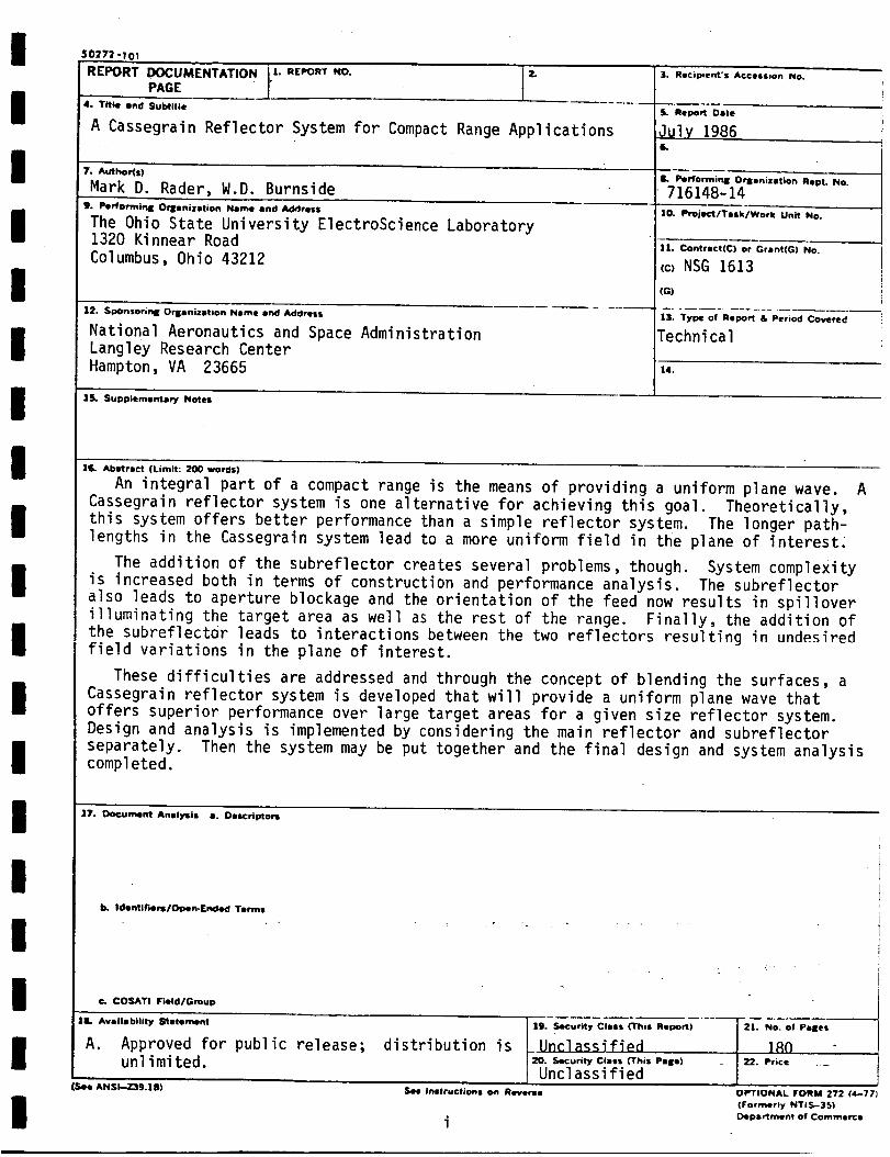
An integral part of a compact range is the means of providing a uniform plane wave. A

Cassegrain reflector system is one alternative for achieving this goal. Theoretically,

this system offers better performance than a simple reflector system. The longer path-

lengths in the Cassegrain system lead to a more uniform field in the plane of interest_

The addition of the subreflector creates several problems, though. System complexity

is increased both in terms of construction and performance analysis. The subreflector

also leads to aperture blockage and the orientation of the feed now results in spillover

illuminating the target area as well as the rest of the range. Finally, the addition of

the subreflector leads to interactions between the two reflectors resulting in undesired

field variations in the plane of interest.

These difficulties are addressed and through the concept of blending the surfaces, a

Cassegrain reflector system is developed that will provide a uniform plane wave that

offers superior performance over large target areas for a given size reflector system.

Design and analysis is implemented by considering the main reflector and subreflector

separately. Then the system may be put together and the final design and system analysis

completed.

27. Document Anelysls II. Descriptors

b. Identifiers/Open-Ended Terms

C. COSATI Irleld/Gmup

IL Ava|leblli_ _eten_ent

A. Approved for public release;unlimited.

distribution isF'-'111. Security Ciess {This Rel:_r&) 1. NO. Of Psl|es

_Unclassified J 1_C} "20. Security Class ('This Pete) i 22. Price 1 --

l

Uncl assi fied ISee AN$1--Z3g.| 8) See InsfruotJons _n Reverse

i

OPTIONAL FORM 272 (4-77)

(Formerly NTIS--] 5)

Depertmen! of Commerce

I

II

I

III

III

I

II

II

I

TABLE OF CONTENTS

LIST OF FIGURES

CHAPTER

I INTRODUCTION

II THEORY

A CASSEGRAIN REFLECTOR SYSTEM GEOMETRY

B MOMENT METHOD ANALYSIS

C UNIFORM GEOMETRICAL THEORY OF DIFFRACTION ANALYSIS

III CASSEGRAIN SYSTEM CONSIDERATIONS

IV THE BLENDED SURFACE

V CASSEGRAIN SYSTEM DESIGN PROCEDURE

VI CONCLUSIONS

APPENDICES

A REFLECTION POINT ON MAIN REFLECTOR

B REFLECTION POINT ON ELLIPTICAL EDGE OF SUBREFLECTOR

C MODIFICATIONS FOR VARIABLE DISTANCE TO PLANE

REFERENCES

iv

1

4

4

918

29

85

148

158

160

160

167

169

172

ill

pRECF..D|tlGPAGE BLAHK NOT Fii.MEO

Figure

LIST OF FIGURES

2.1 Geometry of Cassegrain system.

2.2 Gregorian form.

2.3 Equivalent-parabola concept.

2.4 Scattering problems.

2.5 Placement of test source.

2.6 Sinusoidal strip dipoles for basis functions.

2.7 Nonplanar strip dipole with edges at sI and tI and terminalsat O.

2.8 An electric strip monopole and the coordinate system.

2.9 Probing of a perfectly conducting polygon cylinder.

2.10 Basic UTD field components.

2.11 Curved conducting strip.

2.12 Transition function.

2.13 One face of a general wedge structure is illuminated.

3.1 Parabolic reflector.

3.2 Reflected field.

3.3 Edge diffracted field.

3.4 Edge diffacted field.

3.5 UREF + UDIFF.

3.6 Rolled edge addition.

3.7 UREF + UDIFF.

iv

Page

6

6

8

10

12

14

16

16

17

19

22

25

26

3O

3O

32

34

35

37

40

III

I

II

III

II

III

I

II

I

I

I

I

I

I

I

I

I

I

I

I

I

I

I

I

I

I

I

Fi 9ure

3.8

3.9

3.10

3,11

3,12

3.13

3.14

3.15

3,16

3,17

3,18

3.19

3.20

3.21

3.22

3.23

3.24

3.25

3.26

3.27

3.28

3.29

3.30

Reflected field.

u2REF + uIDIFF.

Subreflector diffracted field.


Caustic distance.

u2REF + U1DIFF + U2DIFF.

Subrefl ector extensi on.


u2REF + uIDIFF + u2DIFF.

Rolled edge addition to main reflector.


Rolled edge addition to subreflector.


Reflected-refl ected-di ffracted field.



Addition of u3DIFF.

Triple reflected field.

Ellipse addition.

Ellipse.

Tilted ellipse.

Addition of triple reflected field.

Spillover incident field and reflected field.

Page

42

46

46

48

48

50

50

51

53

54

56

57

59

DU

62

62

64

64

65

65

65

67

67

Figure


3.32 Spillover field and reflected field additions.

3.33 Target area at variable distance.

3.34 Total field (_)and total field less triple reflected

field( .... ).

3.35 Total field (___) and total field less triple reflected

field (..... ).

3.36 Gregorian subreflector system.


3.38 Doubly reflected field.

3.39 Attachment of ellipse.

3.40 Attachment of ellipse.

3.41 Doubly reflected field.

3.42 Sum of two reflected fields.

4.1 Subreflector with blended surfaces.

4.2 Ellipse for upper edge.

4.3 Ellipse for bottom edge.

4.4 Field along a parabolic contour.

4.5 Physical optics analysis.

4.6 Three integration regions.

4.7 Subreflector with blended surfaces.

4.8 Smaller subreflector with same size surfaces.

4.9 Original subreflector with smaller blended surfaces.

4.10 Far field from subreflector.

vi

Page

68

70

72

72

75

75

76

77

78

78

79

83

86

86

86

91

97

97

99

101

104

106

III

I

II

III

II

III

I

II

I

I

I

I

I

I

I

I

I

I

I

I

I

I

I

I

I

I

I

Figure

4.11 Moment method geometry.

4.12 Field plots for geometry of Figure 4.7 (a).



4.15 Main reflector with blended surfaces.

4.16 Ellipse for upper edge.

4.17 Tilted ellipse.

4.18 Ellipse for bottom edge.

4.19 Parabolic reflector section and field plot.

4.20 Reflector with elliptic rolled surfaces and field plot.

4.21 Reflector with linearly blended surfaces and field plot.

4.22 Reflector with parabolic blended surfaces and field plot.

4.23 Reflector with cosine blended surfaces and field plot.

4.24 Moment method plots for various distances to the

observation plane.

4.25 Reflected field from main reflector.

4.26 Bottom and top reflection points.

4.27

4.28

4.29

4.30

4.31

4.32

Parabolic reflector with blended surfaces.

Parabolic reflector with smaller blended surfaces.

Total reflected field.

Blended surface reflected field.

Entire Cassegrain system.

Entire system.

vii

Page

106

108

109

110

111

111

111

112

117

118

119

120

121

125

130

132

134

137

137

141

142

Figure

4.33 Entire system less main reflector contribution.

4.34 Entire system less main reflector, subreflector and

spillover contribution.

4.35 Desired reflected field.

4.36 GO reflected field.

4.37 Triple reflected field.

4.38 GO triple reflected field.

5.1 Cassegrain system with @v = 35°-

5.2 Moment method plot showing triple reflected field.

5.3 Moment method plot of desired reflected field.

5.4 Cassegrain system with @v = 45°.



5.7 Cassegrain system with @v = 55°.



A.1 Initial reflection point.

A.2 New coordinate system,

A.3 Actual point on reflector.

A.4 Coordinate system transformation.

B.1 Reflection point on elliptical rolled edge.

C.1 Variable distance to plane.

viii

Page

142

143

143

144

145

147

152

153

153

154

155

155

156

157

157

161

161

163

165

168

170

III

I

II

II

II

II

III

I

II

I

I

I

I

I

I

I

I

I

I

I

I

I

I

I

I

I

I

CHAPTER I

INTRODUCTION

Recently, the indoor compact range has received much attention and

is increasng in popularity as it rivals the outdoor range for antenna

and scattering measurements. As the compact range performance improves,

its use will continue to grow. An integral part of this system is the

means of providing a uniform plane wave. This study presents a

Cassegrain antenna feed system as a means to achieve a more uniform

plane wave.

Normally, a single parabolic reflector is used to generate this

plane wave. Edge diffractions are the major drawback to this reflector

system because they generate ripple on the desired uniform plane wave.

One method used to reduce this ripple is through the use of serrated

edges. The edges may also be rolled to reduce the ripple and provide

structural strength as well. Large circular rolled edges provide

greater ripple reduction but require additional structural support and

are more costly. Elliptic edges are also used to control ripple and

these are more effective than simple circular edges since there is more

control over the shape such that a smaller ellipse can work as well as a

larger circular edge. At the bottom of a parabolic dish section,

serrated absorber patterns are often used to break up the field. Proper

tapering of the feed horn field pattern will also minimize the

diffracted fields.

Another possible alternative to the reflector systen_is the use of

a lens antenna. But lens antennas are not being widely used due to

several disadvantages. Although lens antennas are frequency dependent,

the major disadvantage is in the construction of the antenna itself.

Reflector antennas are mucheasier to design since only one surface

needs to be considered. If madeof natural dielectrics, lens antennas

can be heavy and bulky, especially at lower frequencies. The

homogeneity of the dielectric is also often in question. Besides the

structural problems, lenses are also inherently lossy and reflections

occur at both interfaces [1]. Therefore, reflector type antennas are

usually favored over lens antennas.

The alternative considered in this study is the Cassegrain

reflector system. Theoretically, the Cassegrain system offers better

performance than a simple reflector system. The longer pathlengths in

the Cassegrain system lead to a more uniform field in the plane of

interest. The convenient location of the feed and supporting hardware

is another advantage of this system.

Initially, several disadvantages to the Cassegrain system are

apparent. The addition of the subreflector increases system complexity

both in terms of construction and performance analysis. The

subreflector also gives rise to aperture blockage. The orientation of

the feed now leads to spillover illuminating the target area as well as

the rest of the room. Finally, the addition of the subreflector leads

II

II

II

II

III

II

II

II

I

I

l

I

I

I

I

I

I

I

I

I

I

I

I

I

I

I

I

to interactions between the two reflectors resulting in undesired field

variations in the target area. These problems are considered as the

Cassegrain system is designed and analyzed.

The major design consideration in implementing the Cassegrain

system is through the blending of the edges to improve performance as

opposed to simply attaching circular or elliptical edges. The blending

technique is a better method of providing the transition from one curve

to another. Blending also reduces the junction diffracted field and

therefore enhances performance. The tapering of the field is also

controlled through the blending process. In fact, the blending concept

is what allows the Cassegrain system to work as an effective source of a

uni form plane wave.

CHAPTERII

THEORY

A. CASSEGRAINREFLECTORSYSTEMGEOMETRY

The Cassegrain antenna system consists of a main reflector,

subreflector, and feed. The main reflector is a parabolic curve while

the subreflector has a hyperbolic contour. Twofoci are present in

this system: the real focal point located at the feed and the virtual

focal point located at the focus of the parabola. To generate this

system, two variables for each reflector must be specified. Seven

variables are used to describe this system and three equations used to

solve for the three remaining unknowns(Figure 2.1) are as follows:

tan 1@v= _+1Dm_Tl_m (2.1)

1 + 1 = 2 Fctan @v tan@r _ , and (2.2)

1 - sin(@v-@r)/2 = 2 Lvsin(@v+@r)/2 l_ . (2.3)

Equation (2.1) applies to the main reflector while Equations (2.2) and

(2.3) apply to the subreflector. The negative sign applies to the

I

II

II

I

III

III

II

II

i

I

I

I

I

I

I

I

I

I

I

I

I

I

I

I

I

I

I

I

Gregorian forms of the system.

The parabolic main reflector is generated by

Xm = ym2_l_ .

The hyperbolic subreflector is generated by

Xs = a[/l+(_) 2 - 1]

where

e = sin(¢v+_r)/2

sin(@v-@r)/2

(2.4)

(2.5)

(2.6)

a=Fc

, and (2.7)

b = ae2_-1 . (2.8)

.._ =_a_,ons govern th_ classical Cassegrain system, u_,r,9 these

equations, many variations of the basic system may be formed. For this

study, the basic system of Figure 2.1 is sufficient, though one

variation is considered. The Gregorian form occurs when the focus of

the main reflector moves between the two reflectors (see Figure 2.2).

In this case the contour of the subreflector is elliptical. The

negative sign must be used in equation (2.1) since @v is now negative.

Otherwise, the equations remain the same.

In later analysis, the use of the virtual feed is made. In this

concept, the real feed and subreflector are replaced by a virtual feed

Fi gure 2. I

I

IREAL F T

/ . OCAL POIN I/ _" VIRTUAL FOCAL POINT

Ym I

°L !. II

HYPERBOLA I

__t_--_ _,_,.°,,

Fm_C _' I

Geometry of Cassegrain system, I

PAR .. PAR I

t .......... I n"- I

Figure 2.2 Gregorian form.

6

II

II

II

I

II

III

II

I

II

I

at the focal point of the main reflector. The system is now a single

reflector design, and this concept is useful when designing and

analyzing the main reflector.

Another useful concept is that of the equivalent parabola. As is

seen in Figure 2.3, the Cassegrain system is replaced by an equivalent

surface which has a parabolic contour as demonstrated by Hannan [2].

Using this concept, the feed remains unchanged, and ray optics are used

to determine the surface as the locus of incoming rays intersecting the

rays converging to the real feed. Then the Cassegrain system has been

replaced by an equivalent single reflector system. The following

equations show the relationship between the two systems:

1 Dm= tanlcrilF_ _ (2.9)

Xe = ye2, and (2.10)

_+Fe = tan Cv/2 = Lr = e+l

l_m tan@r/2 Fvv _ . (2.11)

Again, the negative sign applies to the Gregorian forms. Equation (2.9)

generates the equivalent focal length. Equation (2.10) generates the

equivalent parabolic surface, and Equation (2.11) provides several

expressions for comparing the focal lengths. For the classical

Cassegrain system, Fe/Fm is greater than one. It is apparent that a

Cassegrain system has a much smaller focal length but can be equivalent

to a single reflector system of much larger focal length. It is this

III

I

Figure 2.3 Equivalent-parabola concept.

idea that favors the Cassegrain system over the single reflector system.

Whenworking in a restricted area, such as a compact range, the shorter

Cassegrain system is favored over the longer equivalent single reflector

system [2].

B. MOMENTMETHODANALYSIS

Several analysis techniques are used when studying the Cassegrain

system. The first that will be described is the momentmethod theory.

Only the two-dimensional part of this theory is outlined [3]. By using

the reaction concept of Rumsey[4], a momentmethod solution may be

obtained. In Figure (2.4) a scattering problem is presented. The

source electrical and magnetic currents (Ji,Mi) generate electric and

magnetic fields (E,H) in the presence of the scatterer which is a

conducting body in free space.

The surface-equivalence theorem of Schellkunoff [5] gives an

equivalent problem by replacing the scatterer by the following surface

current densities:

ds = n x H , and

Ms=Exn

with n being the outward normal to the surface.

(2.12)

(2.13)

It is self-evident that

the source currents (Ji,Mi) generate the incident fields (Ei,H i) in the

free space. The scattered fields are given by

D o D

Es = E - Ei, and (2.14)

9

I

I

I@ ,

(a) s the ) with I

/

(b) The .... )the currents (Js,Ms) I

i

÷ ÷

(c) The exterior scattered field may be generated by (Js,Ms)

in free space.

Figure 2.4 Scattering problems.

10

I m m

Hs = H - Hi . (2.15)

m m

The surface currents generate the scattered fields (Es,Hs) outside them m

body and (-Ei,-H i) inside the body.

An electric test source Jm is now placed within the region of the

scatterer (see Figure 2.5). Because there is no field in this region,

the reaction of this test source with the field produced by the other

sources is zero. By reciprocity, this reaction must be equivalent to

the reaction of the other sources with the field produced by the test

source. Then, one finds that

ff(Js'Em-Ms'Hm)dS + H_(Ji.Em-Mi-Hm)dv = 0 . (2.16)

This equation is the basis of this solution and approach is the

"zero-reaction theorem" of Rumsey [4].

Next, the surface current distributions (Js,Ms) need to be

determined. These currents are constructed of finite series with N

unknown coefficients. For this problem, the scattering body is a

perfect electrical conductor so Ms vanishes. Since only the

two-dimensional case is being considered, Js is a function of the

position _ around the contour of the body. Also consider a magnetic

line source and TEz polarization so that Ji is zero. Then the integral

equation reduces such that

m _ m o

_Js.Em d_ = H Mi'Hm ds . (2.17)C

11

I

I

I#s_,, S

_,_ ,REESPACE./ n%_ _ S w FREE SPACE I

Figure 2.5 Placement of test source.

The electric currents may now be represented by

_ N _

Js(_) = Z InJn(_)

n=l

(2.18)

where In are complex constants, and samples of Js(_) and Jn(£) are the

basis functions. The basis functions as well as the test source have

unit current density at their terminals.

the integral equation yields

N

Z InZmn = Vm with m = 1,2,3,...N

n=l

Substituting this series into

(2.19)

12

where_ n m

Zmn = - fn Jn(_)'Em d_ = -fmJm(_)'En d_, and (2.20)

m m n m

Vm = -HiMi "HmdS = fmJm(_).Eidg (2.21)

with the integrations are done over the non-zero range of the

integrands.

When solving these expressions on a computer, it is advantageous

for the impedance matrix, Zmn , to be symmetrical. Also, the test

sources, Jm, should be the same size, shape, and functional form as them

basis functions Jn. This will allow some of the integrals to be solved

in closed form and yield readily solvable simultaneous linear equations.

In addition, the test sources are placed a distance a from the surface

where a tends toward zero in the limiting case of the integrals. In

this case, sinusoidal strip dipoles are chosen as the basis functions

(see Figure 2.6). This planar strip dipole extends infinitely in the

z-direction and has a surface current density given by [9]

A

J = x sin[k(x-x1)]

sinLk(x2-xl)] (2.22)

for xI < x < x2, and

^

J = x sin[k(x3"x)]

sinLk(x3-x2)] (2.23)

for x2 < x < x3. Similarly, for the strip v-dipole in Figure 2.7 the

surface current density is given by

sin[k(tl-t)]J = -s

sin (ksI) (2.24)

13

III

, I,, I

,I - _ - _ -

I(a) A planar strip dipole with edges at xI and x3 an

terminals at x2. I

I

ii ,1 IL

v v _w _

11 12 13 I

(b) The current-density distribution J on the sinusoidalstrip dipole.

Figure 2.6 Sinusoidal strip dipoles for basis functions.

14

on arm s, and

A

J = t sin[k(tl-t)]

sin(kt 1) (2.25)A

on arm t. It is evident that s and t are perpendicular to the z-axis.

In both cases, the current density goes to zero at the endpoints and is

unity at the center terminals. Also, a slope discontinuity is present

at the center terminals. Of course the v-dipole reduces to the planar

case when _ is equal to 180°.

The field of the strip dipole may be obtained from the

superposition of two strip monopoles considered to have a common

endpoint (see Figure 2.8). The field for the strip monopole is known

from reference [6]. Now the calculation may begin for elements of the

impedance matrix as weii as the Vm elements of the excitation column.

First consider an open or closed perfectly conducting polygon

cylinder (see Figure 2.9). For this open cylinder, surface currents

fluw u_, uu_,, _iJ--u_of _,i_ corlductor, d,u _f_ _urldCe cur reht Ly I

given by Js- A magnetic line source Mi is present and 11 and 12 are the

current densities at the corners of the polygon. Two strip dipole mode

currents may now be defined on the conductor.

point 0 to point 2 with terminals at point 1.

point 1 to point 3 with terminals at point 2.

The first extends from

The second extends from

Each mode has a

sinusoidal current distribution as described earlier. Now the current

density Js is the superposition of these two modes with weightings of 11m

and 12. Then Js is a piecewise sinusoidal expansion with unknown

constants, 11 and 12. Since the polygon is a perfect conductor, the

15

I

I

Y _ I• t i

I

0

SI

X

Figure 2.7 Nonplanar strip dipole with edges at sI and tI and terminalsat 0.

A

I

II

o SOURCE h x !

Figure 2.8 An electric strip monopole and the coordinate system.

16

3

i 2

r 0 I/

| z,

I2

I (a) Perfectly conducting polygon cylinder with parallel

+

magnetic line source Mi.

I

I

i • M i PROBE

i

I

I _ P ROBE I

(b) Electric test probes 1 and 2 are moved to the conducting

I surface.

Figure 2.9 Probing of a perfectly conducting polygon cylinder.

17

tangential electric field is zero on the surface. So, if an electric

test probe is movedalong the conducting surface, the open circuit

voltage at its terminals can be examined. For N different current

samples, N probing tests are done. The probes maybe real (thin wire

v-dipoles) or hypothetical (electric line sources or strip dipoles).

Then the currents I n are adjusted until all the probes read zero.

Finally, as N increases this stationary solution for the currents

approaches the rigorous solution. The mutual impedancebetween the mth

test probe and the nth current modeis Zmn. The probe sumsall them

voltage contributions from Js and Mi and this result must be zero,

resulting once again in Equations (2.19) to (2.21).

Finally, the simultaneous linear equations are solved using linear

algebra techniques, and the current distribution Js is known. The

scattered fields (Es,Hs) may then be found. J.H. Richmond [6] provided

this theory, method, and appropriate computer programs. Using duality,

the TM polarization case could also be solved.

C. UNIFORM GEOMETRICAL THEORY OF DIFFRACTION ANALYSIS

Another analysis technique used is that of the Uniform Geometrical

Theory of Diffraction. Again, only the two-dimensional part of this

theory is outlined.

For the Cassegrain system three basic field components are examined

(see Figure 2.10). These are the incident, reflected and diffracted

fields. The total field is then given by

UTOTAL = UINC + UREF + UDIF (2.26)

18

I

II

!i

I

III

ii

!I

i

iiliI

I

I

iI

I _ _t 7- -! "ooZe"o

RECEIVER i_It'_\ %'%'l_'-Cil'll

I

I

| . .

LINE \ _

SOURCE \ '_e

IMAGE

Figure 2.10 Basic UTD field components.

19

I

where U represents an electric scalar field for the electric line source

case and a magnetic scalar field for the magnetic line source case. The

I

iincident field is given by

-jkPi

C e

t_Regions I and II, and

0 Region Ill

(2.27)

whereas Pi is the distance between the source and receiver. Note that C

is a complex constant. The reflected field is given by

i

II

l-jk Pr

UREF = V_Pr

0

Region I, and

Regions II and III

(2.28)

where Pr is the distance from the image of the source to the receiver

and the positive sign is used for the magnetic line source case and the

minus sign for the electric line source case. To simplify calculations

the magnetic line source is used when analyzing the Cassegrain system.

The diffracted field is given by i

|

iio-i - i ileuDIFF : I P'P ,@-¢', -+ D i P'P ,@+@', C e III_-_-_ I___ T_ _ n

(2.29)

with the plus and minus signs for the magnetic and electric line source

cases, respectively. The term with @-¢' is associated with the incident

shadow boundary while the term with ¢+_' is associated with the

reflected shadow boundary.

20

I

I

I

I

I

I

Ii

I

I

II

I

i

I

I

I

I

Now consider a curved conducting strip as will be found in the

Cassegrain system (see Figure 2.11). The incident field does not change

but the reflected field is now given by

UREF =

D

-jkPi -jkpr-+/ Pc(QR) C e eV Pc(QR)+Pr

0

Region I, and

Regions II and III

(2.30)

with the calculation of Pc(QR) needed. This caustic distance varies

with the reflection point QR and is given by

1 =1 + 2

p-T Rccos 0i (2.31)

where Rc is the radius of curvature of the surface at the reflection

point, QR. The diffracted field is given by

-- i[ -- -jkp' -jkpUDIFF = D [ P'P,¢-¢', -+D I Pc'P ,¢+0', C e e

17_ I_ e'7

(2.32)

!

where Pc is the caustic distance Pc(QE) associated with the reflected

ray from the edge and n=2 such that

-e "j_/4 F(KLa(B))

D(L,B,n=2) =- 2V_r_i_ cos(B/2) (2.33)

21

\\ REFLECTED

\ RAY

RECEIVER \ Y LINESOURCE

II

0

Figure 2.11 Curved conducting strip.

22

II

I

II

i

II

IIII

Ii

I

II

I

F(KLa(B)) = 2jJKL--aX-BTejkLa(B) f_._ e-JT2dT, and(2.34)

a(B) = 2cos2(B/2) . (2.35)

The diffracted field given is sufficient for the knife edge case

but the general form of the diffraction coefficient is also needed. So

more generally, the diffracted field is expressed by

-jkpuDIFF = DS ui (QE) e

H (2.36)

where Ui(QE) is the incident field on the edge, and

-e"j_/4

Ds(@,¢',n) - 2nV2_kH

X

[cot (_+(¢-¢')) F [KLia+(¢-@')] + cot {x-(¢-¢')) F [KLia-(¢-@')]$2n 2n

{cot Cs+(¢+¢')) F [KLrna+(¢+@')] + cot (_-(¢+¢')) F[KLr°a-(¢+¢')]}]2n 2n

(2.37)

where

-j T 2

F(x) = 2j_eJ x fe dT, and (2.38)

23

±(a B) = 2cos2(2n_N+-B)

2 (2.39)

Note that N± are integers most nearly satisfying the following

expressions:

2_nN+-(B) = _, and (2.40)

2_nN--(B) = -_. (2.41)

These expressions are valid for both the soft and hard diffraction

coefficients but only the hard case is used here with a magnetic line

source. The transition function F(x) involves a Fresnel integral, and a

plot of F(x) is shown in Figure 2.12.

The diffraction coefficient may also be written as

DS = D(Li,L i,¢-¢',n) • D(Lrn,Lro,¢+¢',n)H

(2.42)

where

D(L1,L2, @-+@',n) = [cot(_+(¢±¢')) F(KLla+(¢-+@')) +2n

-j_/4cotf_(_+_)_F(KL2a-(¢±_))]e

% 2n j (2.43)

Figure 2.13 shows a more generalized structure. Depending on the

positioning of the line source, reflected fields may emanate from both

surfaces. So two reflection shadow boundaries may exist, and hence the

reason D(Lrn,Lro,@+¢',n) is composed of two terms. The first term is

associated with the n face boundary and the second with the o face

24

II

Ii

I

iIi

i

Iii

Ii

I

II

I

PHASE ( DEGREES )

0 U'_ 0 ul O _ 0 _ 0

II

I

II

I

I

o d

MAGNITUDE

Figure 2.12 Transition function.

25

0

m

0

il

I

Il

I

_,. ._.,_.. I

CURVED FACE_, /___ /

//, I

II

Figure 2.13 One face of a general wedge structure is illuminated, i

!

26 |

!

I

I

I

I

I

I

I

II

I

I

I

I

I

I

I

I

I

boundary.

are measured. The n face is the opposing surface.

The o face is defined as the face where the angles @ and ¢'

Also, the range

parameters are given by

• and (2.44)

nLrn = PcP

-TrT--Pc+P

OLrO = Pcp

pc%T÷p (2.45)

n owhere Pc and Pc are the caustic distances for the reflected waves

emanating from the edge for the n and o faces, respectively. Similarly,

two incident shadow boundaries may exist, and two terms are also

associated with these. In this case, the range parameter is given by

Li = p'pT

p +p (2.46)

Thi S .... 1 ^_- _-,........ _._ the baslc theory and ,,,u,_detailed analysis may be Found

in the class notes by Burnside [7] for microwave optics. In later

chapters some additional details of the theory are needed• and they are

presented when needed.

One final technique used in this analysis is physical optics. This

involves rather simple analysis and will be described later when

actual ly implemented.

The three analysis techniques may now be compared to see the

advantages and disadvantages in each for analyzing the Cassegrain

system. The Uniform Geometrical Theory of Diffraction (UTD) requires

27

analysis of the geometry which may or may not be easily implemented.

Including enoughterms to accurately predict performance may be

difficult but if possible, UTDprovides results with very little

computation time required. The UTDis also well suited for large

electrical objects such as the Cassegrain system. If results are

consistent with other techniques, UTDmaybe used as a valuable design

tool becauseof its high frequency capability and ease of computation.

The physical optics technique is also easy to implement and its results

maybe easily comparedwith the other techniques. Physical optics is an

approximation though, and this is a limitation. Finally, the moment

method technique provides the greatest accuracy but at the expense of

ease of computation. Muchcomputational work must be done so moment

method results require muchtime and space on a computer. The moment

method is also limited by object size. In the case of the large

Cassegrain system, this limits the upper frequency that maybe examined.

Since the momentmethod provides accurate results, it maybe compared

with UTDto see what field componentsare dominant. So the faster UTD

may be used to initialize a design and the slower momentmethod to

finalize it. The momentmethod will also give more accurate results at

lower frequencies; whereas, UTDmaybe used to predict the high

frequency behavior.

28

II

II

!I

ii

I

IIi

!I

I

II

I

II

II

I

l

III

lII

I

i

III

CHAPTER Ill

CASSEGRAIN SYSTEM CONSIDERATIONS

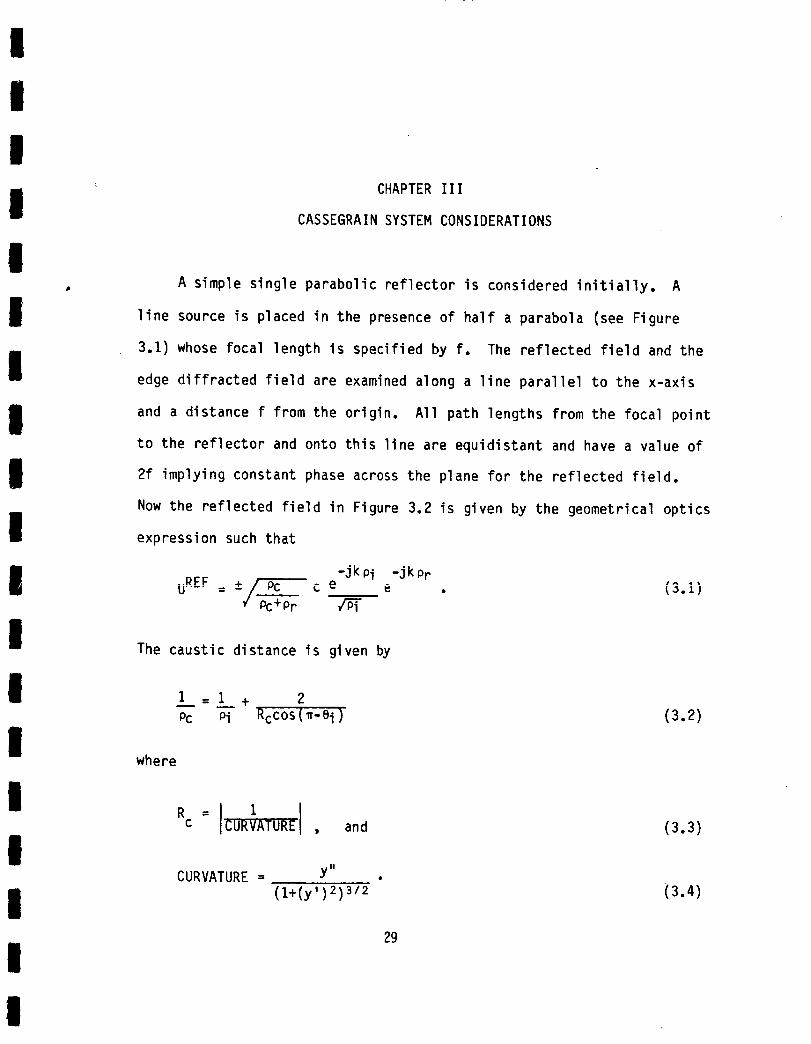
A simple single parabolic reflector is considered initially. A

line source is placed in the presence of half a parabola (see Figure

3.1) whose focal length is specified by f. The reflected field and the

edge diffracted field are examined along a line parallel to the x-axis

and a distance f from the origin. All path lengths from the focal point

to the reflector and onto this line are equidistant and have a value of

2f implying constant phase across the plane for the reflected field.

Now the reflected field in Figure 3.2 is given by the geometrical optics

expression such that

-jkpi -jkpr

P_ +/ Pc c e .^u.... : e . _.i)

_pc+Pr vr6T

The caustic distance is given by

1 =1 + 2

Pc Pi Rccos (_-Bi) (3.2)

where

Rc , and (3.3)

CURVATURE = Y" •

(1+(y')2)3/2 (3.4)

29

X2

4f

III

IX

Figure 3.2 Reflected field.

30

m

II

II

Solving these expressions for Rc, one finds that

Rc_-12f(1+x21(4f2)_3121 (3.s)

In addition, one obtains the following:

c°s(20i) = Pc/Pi

cos20 i = (1 + cos(20 i)/2

II

III

cosO i = lCl+pr/p i)/2 .

cos(_-o i) = -coso i , and

Pr + Pi = 2f .

Substituting thse into Equation (3.2), one obtains

PC = 1 . 1

Pi frl+x213z2[f__llZ24-T_" piJ

(3.6)

(3.7)

(3.8)

(3.9)

Now

or

Pr = f - x2/(4f)

P_L= 1 - x2f 4f 2 .

(3.1o)

I

II

i

Substituting this result into Equation (3.9), one finds as expected

that

Pc = ® , and (3.11)

31

with

UREF= ± c-jk(pi+p r)

e (3.12)

II

IPr = f - x2/(4f) , and (3.13)

Pi = _xZ + Pr "(3.14)

Now UREF is known as a function of x.

The edge diffracted field in Figure 3.3 is given by

!

UDIFF = rD(P'P ,¢-¢',n) -+ PcP -jkp' -jkpL _ D(p___, @-@',n) ]c e e

(3.15)

II

l

I

Pc Y-_

x 4f a I

I

I' I

f

Figure 3.3 Edge diffracted field.

32

III

lI

I

I

IIIII

I

II

II

l

Since n = 2 in this case, one finds that

-j_/4

D(L,B,n=2) = -e F(kLa(s))242_-k- cos(B/2) (3.16)

jkLa(s) ® -jT 2

F(KLa(B) = 2jAT[_ e fvlT[ e dr, and(3.17)

a(S) = 2cos2(S/2) . (3.18)

From Figure 3.3, one obtains

p' = Va_ + (f - a_14f) A , and (3.19)

l

PC = (3.20)

as calculated earlier. Also, the following expressions are found

p2 = x2+(p,)2 _ 2xp'cose"

o" = w/2 - e'

e' = sin-l(a/p')

cos(_/2 - e') = sine'

sine' = a/p' , and

p = (x2 + (p,)2 . 2xa)I/2 .

Now @' and @ need to be determined.

fol lowing:

(3.21)

From Figure 3.4, one obtains the

sin(2ei) = a/p'

ei = 1/2 sin-l(a/p ')

@' = w/2 - ei

(3.22)

(3.23)

33

x2 = (p,)2 + p2 _ 2p'pcosy

Y cos-Z(_x2+!p)2+ p2)2p p

@=_' +y

B-=¢-@'

B" =Y , and

(3.24)

(3.25)

(3.26)

II

l

I

I

B+ = ¢ + ¢' .

Substituting Equations (3.25) and (3.23) into (3.22), one finds that

B+ : x - sin-l(a/p') + y . (3.27)

I

• o |

II

, |

Y |

Figure 3.4 Edge diffacted field.

34

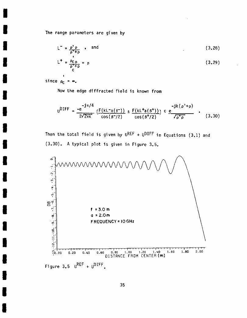
The range parameters are given by

L'= plp

!

L+= Pcp

c

l

since Pc = =.

• and

= p

Now the edge diffracted field is known from

(3.28)

(3.29)

-j_14

uDIFF = -e (F(RL-a(B-)) +_ F(RL+a(B+11_

2v' cos(B-/2) cos(B+I2)c e

-jk(p'+p)

(3.30)

Then the total field is

(3.30). A typical plot

given by UREF + uDIFF in Equations

is given in Figure 3.5.

(3.1) and

i

°.

r'_ i :

i

i

i

(5i

m-}

,-TO.O0

f :&Ore

o :20m

FREQUENCY : I0 GHz

' ' ' "1 ' ' ' ' I ' ' ' " I ' ' ' ' I .... i ' ' ' ' I ' ' ' ' I ' ' ' ' | ' ' ' ' i ' ' ' ' I ' '

O. 20 O.qO O. 60 0.80 !. O0 t.20 1 .qO !. 60 1.80 2. O0

DISTRNCE FROM CENTER (m)

Figure 3.5 UREF + UDIFF.

35

Nowthe addition of a rolled edge is madeto the parabola to reduce

the ripple generated by the diffracted field (see Figure 3.6). The

diffracted field at the junction must nowbe recalculated. More

generally, one obtains that

-jkpuDIFF= DS ui(QE) e

H

i (QE) = cvT_

(3.31)

(3.32)

DS = D(L i,Li,@-¢',n) _ D(Lrn,Lro,¢+¢',n), andH

D(L1,L 2,¢-+¢',n) = [cotIT+(¢-+¢'))F(kLla+(¢-+¢'))2n

-j _/4

+ cot (_-(¢+¢'))F(kL2a-(¢_+¢'))]2n e

(3.33)

(3.34)

The distance given by p and p' have been previously calculated but the

two terms of DS need to be considered.H

finds that

Looking at D(Li,Li,¢-¢',n), one

-jx/4D(L i,Li,¢-¢',n) = -e

2nV_Z_-_-[cot(T+(¢-¢'))F(kL ia+(@-¢'))

2n

with

+_otC__ _))F(k,_(_))]

n =1

(3.35)

(3.36)

Li = p'p (3.37)

36

I

iI

ig

I

Ii

!iI

II

II

II

!

I

I

i

I

I

I

I

I

I

l

I

I

I

I

I

l

I

l

\

0

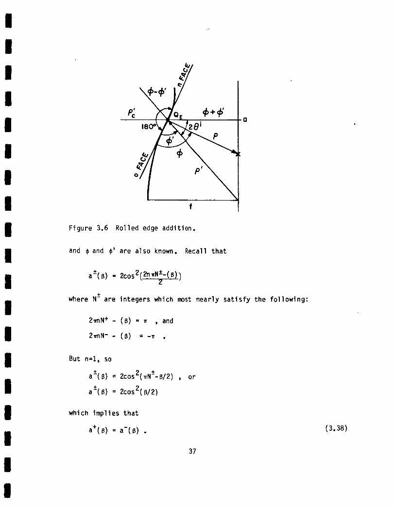
Figure 3.6 Rolled edge addition.

and @ and ¢' are also known. Recall that

a-+(S) = 2cosZC2n_N_-(B))

+

where N- are integers which most nearly satisfy the following:

2_nN + - (B) = _ , and

2_nN- - (B) = -_ .

But n=l, so

+(a B) = 2cos2(_N-+-B/2)

+(a B) = 2cos2(B/2)

or

which implies that

a+(8): a'(8)

37

(3.38)

Inserting Equation (3.38) into (3.35) yields

D(L i,Li,¢-¢',1) =

-j_14-e

2V7_{cot(_12 +(@-¢')12)

+ cot(_/2 -(¢-¢')/2)} F(kLia+(¢-@ ') . (3.39)

From the geometry, one finds that

cot(_/2 + _) + cot(_/2 - m) = cos(_/2 + _) + cos(x/2 - m)sin(_/2 + _) si-n(_/2 - _)

= -sinm + sinmCOSOt COSo_

=0.

Thus, the incident shadow boundary terms are given by

D(Li,Li,¢-@',I) : 0(3.40)

Now looking at the remaining terms, one obtains

D(L rn Lr° ¢+¢' 1) =' ° '

2/7_-[cot(_/2 + (@+@')/2)F(kLrna+(@+@'))

+ cot(_/2 - (¢+@')/2)F(kLr°a-(¢+@'))]. (3.41)

But as before,

a+(B) = a'(B) = a(B) (3.42)

38

I

Ii

II

IIII

I

III

I

I

L

I

I

lIi

II

I

Ii

!l

!II

I

Ii

I

I

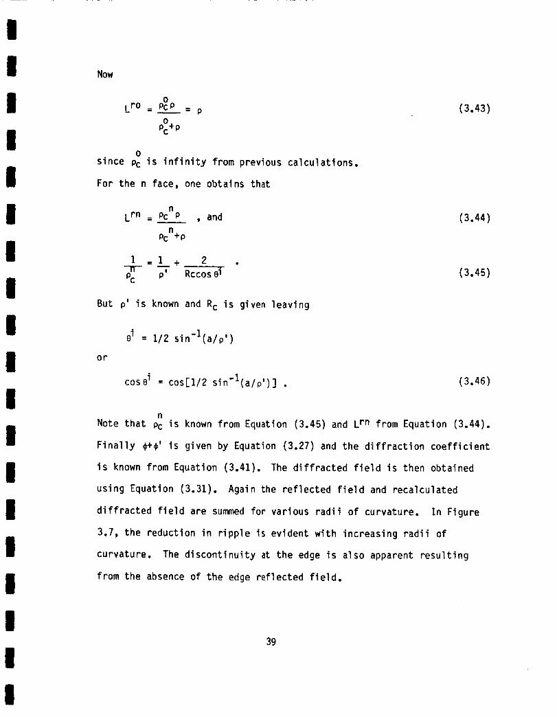
Now

ol rO = PcP --- p

0PC + P

0

since Pc is infinity from previous calculations.

For the n face, one obtains that

n

Lrn = Pc P , and

pcn+p

1 =1 + 2

--IT- p, eiPC RCCOS

But p' is known and Rc is given leaving

ei = 1/2 sin'l(a/p ')

or

cose i = cos[I/2 sin'l(a/p')] .

(3.43)

(3.44)

(3.45)

(3.46)

n

Note that Pc is known from Equation (3.45) and Lrn from Equation (3.44).

Finally @+@' is given by Equation (3.27) and the diffraction coefficient

is known from Equation (3.41). The diffracted field is then obtained

using Equation (3.31). Again the reflected field and recalculated

diffracted field are summed for various radii of curvature. In Figure

3.7, the reduction in ripple is evident with increasing radii of

curvature. The discontinuity at the edge is also apparent resulting

from the absence of the edge reflected field.

39

¢r

v;"

i'_ °-

¢0

o;'

6i°,

i° •

7

o= 2.Ore

FREQUENCY = IOGHz

Rc= 0.125m

i

.... I .... I ' ' ' ' I .... I .... I .... ! .... I ' ' ' ' I .... I .... I ,1•0 0.2 O.Li 0.6 0.8 1.0 1.2 l.q !.6 1.8 2.0DISTANCE FROM CENTER

(a) Rc = 0.125 m.

._

= :

f_

=."f,.

i°.

i

=:

7.;i°--

m q

T_

u_

i.

i •

Figure

f = 5.Ore I

o =2.Ore

FREQUENCY = I'OGHz

Rc= O.5m

!I

I

\

' " '' I .... I .... I ' ' " ' I .... I .... I ' ' ' " ] .... I ' ' " ' I .... I ' '

0 0.2 O.Id 0.6 0.6 I.O 1.2 i.q 1.6 1.8 2.0DISIRNCE FROM CENTE_

3.7 uREF + uDIFF.

(b) Rc = 0.5 m.

4O

II

II

I

II

II

III

II

I

II

I

I

I

I

l

I

I

I

I

I

,°

o.

&"

°o

o

.o

0 i •

f =3.Ore

o =2.Ore

FREQUENCY = IO GHz

Rc= 2.Ore

'''' 1 '' '' I' ''' I '' '' 1'''' I'' '' 1'' '' 1''' ' I'''' I ' ' ' ' I _ '

0 0.2 O.Y 0.6 0.8 l.O 1.2 ].U, 1.6 1.8 2.0

DISTANCE FROM CENTER

(c) Rc = 2.0m.

Figure 3.7 (Continued).

Now consider the Cassegrain system. The governing equations have

II

II

previously been described in the theory section. Again, the reflected

field is analyzed first (see Figure 3.8) and is given by

-jkPi -jk PiuREF= / Pcl c e e . (3.47)I v

Pcl+Prl

The reflected field caustic position is calculated easily from the

following geometrical considerations:

i 2 = (LV.Xs)2 2Pc1 + YS

2 2

I Pi = Ys + (Fc'Lv+xs)

I 2 (ym_Ys)2 _ (LV_Xs))2Prl = + (Pr2 •

(3.48)

2• and (3.49)

41

(3.50)

Now it is necessary to relate Ys in terms of Ym, the desired field

point. First, one obtains that

Pr2 = Fm - ym2/(4Fm) (3.51)

xs = a [,/1 + (Ys/b) z - 1] , and (3.52)

tan a = Pr2 = Lv-xs

Ym Ys • (3.53)

Substituting Equations (3.51) and (3.52) into (3.53) yields

a_l i _

Lv2 + 2aLv

+ (bCl)2Ys = Lv + a - (3.54)

cI - (I/Cl)(a/b)2

where

cI(3.55)

Pc,/_. P,, =

L L LvFc _-r-- F ;-

m

Ym

Ys


42

III

II

I

II

II

II

III

I

II

So now Pc1, Pi, and Prl are in terms of Ym, and UREF may be

calculated from Equation (3.47). Then, the reflected field along the

observation line is given by

I uREF = uREF e-jkPr2

I since Pc2 = ®. Note that Pr2 is given by Equation (3.51).

(3.56)

I

l

I

I

The diffracted field from the main reflector edge is computed now.

As with the parabolic problem, one finds that

-jKp

u_IFF = UlE'REFe [OC(_Er1+E _c2_Pc1)P ,¢+@',n) + DC__,¢+C',n)]

E + E Pc2+PPrl Pcl+p

(3.57)

where

/_ E EE _jkpi _jkpr 1

nREF = c e e

_IE V ,E..,,E• "Cl Vrl "_i

(3.58)

E

Pc =_ ELv-xs)2+(Ds/2) 2

(3.59)

I

II

xs : a -I]

E :_Ds/2)2 Fc.Lv+x_)2Pi + (

(3.60)

(3.61)

43

y_( E (Lv.x_))2E Dm/2-Ds/2)2 + (Pr2" andPrl =

EPr2 = Fm- "'(Dm/2)2 .

4_m

Again, the diffraction coefficient consists of terms as follows:

-j_/4

D(L,B,n=2) = -e F(kLa(B))2_-_-_'_cos (B/2)

and

a(B) = 2cos2(B/2) .

From parabolic edge calculations, one obtains that

E E 2p = (ym2 + (Pr1+Pcl) -YmDm) I/2

Pc2 : ®_

!

B-=¢-¢

[_ym2+( E E 2 2B" = cos -1 P 1+Pc1) + P ]E E

2( Prl+Pc i)p

B+=¢+@ '

B+ 1 Dm=x-sin- + B"

E E2(Prl+Pcl )

E E

L- = (Prl+Pcl)p

E E(Prl+Pcl+P)

, and

44

(3.62)

(3.63)

(3.16)

(3.18)

(3.64)

(3.65)

(3.66)

(3.67)

I

II

Ii

I

igg

II

III

i

iI

I

I

I

I

I

I

I

I

I

l

I

I

l

I

I

I

I

I

I

L+= p (3.68)

since Pc2 = ®- So finally, the diffracted field is given by

u_IFF .REF= UlE

-jkp -j_14e -e

2J-p'p 2/2_k

[F(kL-a(B-)) + F(kL+a(B+))] .

cos(B-/2) cos(B+/2)

(3.69)

The sum of UREF and UDIFF is shown in Figure 3.9 for one example.2 1

Another major field component is the diffracted reflected field

from the subreflector edge (see Figure 3.10). This field is given by

E-jkPi -jk Pl E

u__FF:IO_ {__ __ _ [D(_I,_-_,2)_P2 /pE P_I E.

YPc

Pi Pl

E -jkP2+ D(_cpl,_+_',2)]}e

oE+o.'C "I

f_ 7n_

with

-j_14

D(L,B,n=2) = -e F(kLa(B))

2v_ cos(_/2) (3.16)

and

a(B) : 2cos2(B/2) . (3.18)

45

II

I

'?,

=, Dm : 40m I_, Fm : 30m

_= Fc : 2.5m

_' Ds : 1.0 m I

=' FREQUENCY : IOGHz

' II, _l_-;_-_,_.=-rr_ r-r --rr r-rT.r,

0.6 0.7 0.8 0.9 I.O l.i 1.2 1.3 1.._ 1.5 I._,'_0.5 6 1.7 1.8 t.9 2.0 2. t

DISTRNCE FROM CENTER I

Figure 3.9 U2REF + uIDIFF.

!

!

!l

!

i !

Figure 3.10 Subreflector diffracted field.

46

The geometry for this field analysis is given in Figure 3.11. The

I

I

s2= (Xm-

needed relationships between the various parameters are given as

follows:

XE 2m = (Dm/2) /(4Fm)

(Fm-Fc)2) 2 + (Dm/2)2

I

II

II

IlI

I

I

oi i/_cos-l[(p_)2+(°Erl)2-s2= ]E E

2Pi Prl

(_' : It . O.

(s ')2 = ym2 + (Fm-Fc-y2/(4Fm) 2

m

B = ¢-¢' = cos-1

4-

B = ¢+¢' = B- +_-20.1

EL- = PiP1

E+Pi Pl

EL+ = PcPl

pEc+Pl

, and

Now Pc in Figure 3.12 is given by

I__: I___+ 2PC Pl RcC°S (_-Oi)

47

(3.71)

(3.72)

(3.73)

(3.74)

(3.75)

(3.76)

_.77)

(3.78)

(3.79)

(3.80)

!II

/l__

I

i

Figure 3.11 Subreflector diffracted field. I

I

/ I I

/ / i JI

I

Figure 3.12 Caustic distance.

48

and

2 (4Fm2)3/21Rc = 12Fm(l+Ym/ (3.81)

II

I

II

from Equation (3.5). The reflection point is found from an iterative

routine given in Appendix A. Now uDIFF is known from Equation (3.70).2

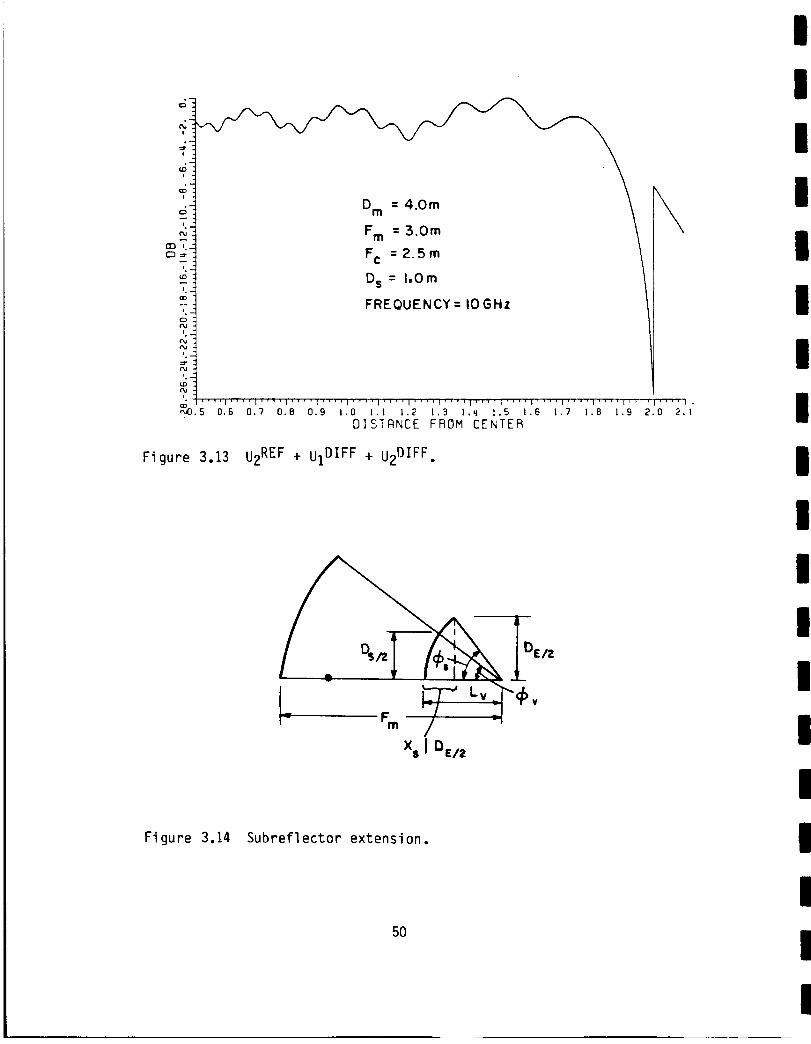
The sum of UREF, UDIFF and UDIFF is given in Figure 3.13 as a sample2 I 2

geometry.

The discontinuity in Figure 3.13 may be alleviated somewhat by

extending the subreflector and reducing doubly diffracted fields (see

Figure 3.14). The subreflector size is now determined by Cs; whereas,

DE may be found from

TAN@ s = DEI2

v_'xSlDEl 2

(3.82)

Inserting the system parameters into this equation and solving for DE

i yields

i DE = (TAN@s) [a+Lv+-Va2+(2aLv+LvZ)((aZTANZcs)/b z)]1 . a2TAN2¢s

2 2b2

I with the minus sign giving the desired solution.

(3.83)

II

I

II

The diffracted reflected field may now be recalculated (see Figure

3.15) using

DEED

Xs = a[_- I] (3.84)

DEED / DEED)2p. = (DE/2)2 + (Fc-Lv+x s (3.85)1

49

T

CDi

t

_r

t .

i

c'd

F,

Fm =30m I _

Fc =2.5m / /D s = l,Om 1

FREQUENCY= IOGHz

_J_.,_''_'_'_'_'_'__'_i'_'''_'_'''_'_''_'''_ .... I.0.6 0.7 O.B 0.9 1.0 1,1 1.2 1.3 1.4 1.5 1.6 1.7 l,B 1.9 2.0 2.1

D]STRNCE FROM CENTER

Figure 3.13 u2REF + uIDIFF + U2DIFF.

D EIz

Fm _-'_J Lv_ _'(_v

xs I DE/2

Figure 3.14 Subreflector extension.

50

I

I

I

I

l

I

I

I

I

I

I

I

I

I

I

I

I

I

I

II

II

I

II

III

II

II

II

I

I i / P-_,v_lI L F, 21i_ F" Fm c a

Figure 3.15 Subreflector diffracted field.

DEED / 2 ,, DEED,2Pc = (DE/2) + tLv'Xs ) , and

DEED

-jkp i -jkp 1e e

/jE0

DEED -jk P2+ D(Pc Pl ,¢+¢',2)]}e

DEED+Pc Pl

In this case, one finds that

DEED

[D(._ Pl

DEED+Pi Pl

20i =_-_

where

DEED DEED 2 2

a = cos'l[(pi )2+(pc ) -Fc ]

2P_ EED pcDEED

51

,@-@',2)

(3.86)

(3.87)

(3.88)

In addition•

¢' = _12 - 0i. (3.90) I

Again• B" is given by Equation (3.76); whereas•

B+ = @+¢' = B-+a. (3.91)

The sum of UREF uDIFF DIFF• 1 and U is again shown in Figure 3.16. The

reduction in the discontinuity is obvious.

To reduce the ripple• a rolled edge is now attached to the main

reflector (see Figure 3.17). The analysis is similar to the single

reflector design discussed previously. First• the diffracted is given

by

and

-jkp

U_ IFF = D Ui(QE)e¢_ -

(3.92)

ui(QE) = u_EFIQ E

which is known from Equation (3.58) and those that follow.

obtains the following:

(3.93)

Agai n, one

I

II

Lro = p (3.94)

n

Lrn = pcP (3.95)

npc + p

52

_D

°.O_,

13DCD

z_

Fm = IOOX /

Fc = 8OJk

_6s = 35 °

_t`_17._9_2]_23_2_27_9_31_33_35_3_q_q3_q5_q9_5I_53_55_5_59_6_.63_65_

D]STIqNCE FROM CENTER

i

=;-

I

I

i .

i°.

(a) +s : 35°-

_:)V= 35o \

_r = 15°

F m = IOOX

Fc =BoX

(_s : 40o

\

.... I .... i .... 1.... I .... I .... I .... I .... 1 .... I .... I_"'I .... I .... I .... I .... I .... ! .... I'"'l .... l''"l .... I .... I .... I .... l'"_l _''"

_/:5.]7.19.21.23.25.27.29.3].33.35.37.39. ql.q3.45.LlT.q9.51.53.55.57.59.61.63.65.


(b) Cs : 40°-

Figure 3.16 U2REF + UIDIFF + U2DIFF"

53

o-

r

t

t

i

i

rn

t

t

to.

f_a

I

Figure 3.16

i6, = 15° \

F m : I00>, \

F c : 80>_ \

(_S = 45°

(CHANGE IN dB SCALE)

"'I''"l''"l .... I''"I""I''*'I .... I .... I .... I .... I''"I .... I .... I'"'I .... I""I .... l .... I .... I''"I"''I .... i .... l''"I ....

7. 19' 2] " 23" 25" 27- 29. 31 . 33. 35. 37.39.4l .43.45.47.49.5]. 53.55.57.5g. 6]. 63.65.


(c) Cs = 45°.

(Continued).

I

I

I

I

I

I

1

1

I

1

____ ] 1'_ II_. Fm _ !

I_ _ I

Figure 3.17 Rolled edge addition to main reflector.

54

I

II

1 =1 + 1

p-T Rccos oipc

E EPi = Pc + Prl '

and

(3.96)

(3.97)

i = 1 sin-1

Dm(3.98)

I

I

I

Then, the diffraction coefficient is given by

-j714

D = -e

22v_-_k_k[cotC_/2 + (@+@')/2)F(kLrna(_+¢'))

+ cot(_/2 - (@+@')/2)F(kLr°a(@+@'))] (3.99)

and UDIFF is known from Equation (3.92). The effect of increasing Rc

the reduction of the fast varying ripple is shown in Figure 3.18.

The slow varying ripple may now be reduced by attaching a rolled

on

edge to the subreflector (see Figure 3.19).

that

IFF _ "jkP2U = c UDIFF e

In this case, one finds

(3.100)

where

DEED

-jkpi -jkp IUDIFF = c e e D. (3.101)

In addition, the range parameters are given by

I

II

DEEDLro = Pc Pl

DEEDPc *Pl

55

(3.102)

i

°-

i

=6-t

_

i "

t_

rn i _

c__=-

m."

*.Z

_Jt'U

i. 7

I

J

i

i "

:7 Z

r_

f'a

Cu

(%

Figure

_r=,50 \Fm = IOOX 1

FC = 80_, 1

_s = 35° 1RCMAIN = 0

.... J'''ll .... I .... J .... I .... I .... I .... I .... I .... I'"'1 .... I .... ]''"1 .... I''"1""1 .... I""l'"'l""l .... I''"1'"'1 .... l ....

7.19.21.23.25.27.29.3].33.35.37.39._I.W3.W5.47. q9.51.53.55.57.59.61.63.65.


(a) RcMAIN= O.

_ ,oox II\Fc = 80),

_S = 35°

RCMAIN = I0_.

.... I'"'1 .... I .... I .... I .... I .... l''"l'"'l''"l .... I .... I .... I .... I""1'"'1""1'"'1""1 .... _ .... I .... I""1'"'t .... I ....

]2. 19. 21. 23.25. 27. 29. 31. 33. 35. 37. 39. WI . q3. _5. qT. q9. 51. 53. 55. 52. 59. 6]. 63. 65.


(b) RcMAIN = fOX.

3.18 u2REF + uIDIFF + u2DIFF.

56

I

lI

II

I

II

III

II

I,I

II

I

n7

(7

i

°-

i

°o

t

_V = :55o

_r = 15°

Fm = I00_,

F = 80Xc

=55 °$

RCMAIN = 50X

(CHANGE IN dB SCALE)

-_75_17_9°21_23`25_2_`29`3t`33_35_3_39_q3_q-_`9_5_53_55_5_59_l_3°6_

DISTFINCE FROH CEN]ER

(c) RcMAIN = 50X.


F- m

Figure 3.19 Rolled edge addition to subreflector.

57

Lrn =

I Z

m

nPc

nPcPl , and

nPc + Pl

1 + 2

DEED RccoseiPi

(3.103)

(3.104)

As before,

2ei =_-

where

ot = COS -I [.( pDEED) 2 + (pcDEED)2 . Fc 2]DEED DEED

2Pi Pc

(3.105)

(3.106)

The diffraction coefficient is given by

-j _14

D = -e

2/2_k[cot(_/2 + (¢+¢')12)F(kLrna(@+@')

+ cot(_12 - (@+@')12)F(kLr°a(@+@'))] (3.107)

and B" is given by Equation (3.76) and

B+ = @+@' = B-+a • (3.1o8)

The new diffracted reflected field is then given by Equation (3.100).

The effect of increasing Rc on the reduction of the slow ripple is shown

in Figure 3.20.

Another field component that needs to be considered is the

field (see Figure 3.21). U_EFreflected-reflected-diffracted has been

computed previously and is given by

58

I

II

II

I

II

III

II

II

II

I

_r = I'_°

Fm= IOOX

. Fc " 80_

,4

' RCMAIN = IOOX

"," _CSUB• o _h _D]:)IRN[[ FROH [ENII:FI

(a) RcSUB = O.

I

_v = 35°

i _ ¢r : 15° \

F m = I00),

F : 60},c

£.hc_

45 = 35 o

Ii

I

RCMAIN = IOOX

RC SUB = 5;k=r

i -

¢r.b

I:_ ' '"1 .... I .... I .... I .... r¢"l .... I .... I' "tT"lVlTtr_trrml"_WTrrMl"_'l" '1 .... I .... rm_'l_t'l .... I .... 1 .... I .... I .... } .... I'"1

4-`5.!_9_5_3_3_3q_6_b_q_?_qB_5__5_6|_3_5_6 7.

DISTRNCF FHOM t'ENIEP,

(b) RcSUB = 5X.

Figure 3,20 U2REF + uIDIFF + u2DIFFo

I

iI 59

I

I

t

CZ) c_

+

i

i

i

Figure

I

I+v=-° ......_\

F m = I00 X t

_s = :35°

RCMAIN = IO0_ / I

.cso_;,_× _ iII

r'+" I .... I'"'I .... I .... I i ' _ l"TTTl-rI"q I" "rr_r I _ r_ "T'rlTT T'rr'Fr'rlTFrr_ 1 .... i .... I .... rcrr"l'rr+rq_ + r+ ,r'_ '_ 1 T+ r +37. 19.21 23.25.2 .28.30.32.3_.:,6. _O.40.42.44.4t,.qB.SO.S2.54.bG.57.55.6].G3.f'_.L-.

DIS[ANEI FHOH CENIEFI I

(c) RcSUB = 25x.

3.20 (Continued). I

I

!

I/ /

D -,-_ l t_EDGE REF p _1 i

Figure 3.21 Reflected-reflected-diffracted field.

60

I-jkpEDGE

m uREF = uREF e(3.109)

Now, the reflected-reflected-diffracted field is given by

-jkp DEED

U_ IFF U_EFe= V'_ [D( p, ¢-¢',2) + D (Pc PpDEED+p ,¢+¢',2)] (3.110)

with D(L,B,n=2) as before. From Figures 3.22 and 3.23, one obtains the

fol lowi ng:

EDGE DEEDP2 = Fm-Lv + xs - " " ""tDE/2)2/(4Fm) (3.111)

p = [(y-DE/2)2+(Lv_x_EED)2]I/2(3.112)

B- = ¢-¢' = _ - sin "1 (y-DE/2)p

(3.113)

O. = COS .I[(pDEED)2+ (pDEED)2_ Fc 2]

2p_EED DEED (3.114)Pc

y = _/2 - ei , and

¢' = y + sin "1 DE/2 ] •J

Pi _J

Now, the diffraction angles are given by

S+ = ¢+¢' = B" + 2¢' , or

i /B+ = B" + a + 2sin -1 DE/2 ] .

i JJ_Pi _J

(3.115)

61

Figure 3.22

Figure 3.23

/

II

II

_oo_ ___, ' I

IReflected-refl ected-di ffracted fleld. I

I 2__oE, 2 |

'o-/ "i I

Refl ected-refl ected-di ffracted field.

62

that U_IFF follows from Equation (3.110), A typical plot Is shownNote

in Figure 3.24 that also includes the previously calculated terms.

As can be seen In the previous figure, the knife edge is

undesirable. An elliptical rolled edge Is now attached to the

subreflector to eliminate the reflected-reflected-diffracted field and

reduce the diffracted-reflected field at the expense of introducing a

triple reflected field (see Figure 3.25). This field will be analyzed

next. UREF has been calculated previously and

-jk P2

UREF . UREF e (3.116)

where P2 must be determined. Now the normal of the hyperbolic

subreflector is given by

. /b2)yn =x s . (a S S

ir1+(Ys/b)_i

2' _#Sl u I

(3.117)

and the center of the ellipse is specified by

A A A A

XEXs+YEYs = xs(DE/2)x s + (DE/2)Ys+Bn (3.118)

(see Figure 3.26).

x = Acosv, and

y = Bsinv

Now the ellipse is paramaterized by

(3.119)

(3.120)

for 0 < v < 2_ (see Figure 3.27). Tilting the ellipse and shifting its

center result in Figure 3.28, and one obtains

63

°,

=,

=,

=,.

0 =

t .

I

m

I

I

_o=,oo_ \ !iF¢ = sox /

_= = 3s° ' i

t

ru

I' ' ] .... I .... I .... _ ' ''1 .... I .... I .... I .... I .... I .... I .... i''''i .... I .... I .... I .... I''''1 .... I .... ] .... 1' ''1 '''1''' i .... I'" "

_r._. 17. 19.2]. _3.2to. 27._9. 31.33.35. 37. 39- _1 . 113._5. wT. _9.51. -_'3-55.57.5b. GI. g3. L 5"

' DISIANCE FF-_OMCENTER

Figure 3.24 Addition of u3DIFF.

I

I

1

!

Figure 3.25 Triple reflected field.

64

I

I

"I X$ ( DE/2 ) Xs

IFigure 3.26 E111pse addition,

II

!

Figure 3.27 Elltpse.

I

I '_'i _, Y_ )

Ftgure 3.28 Tilted elllpse.

65

I

with

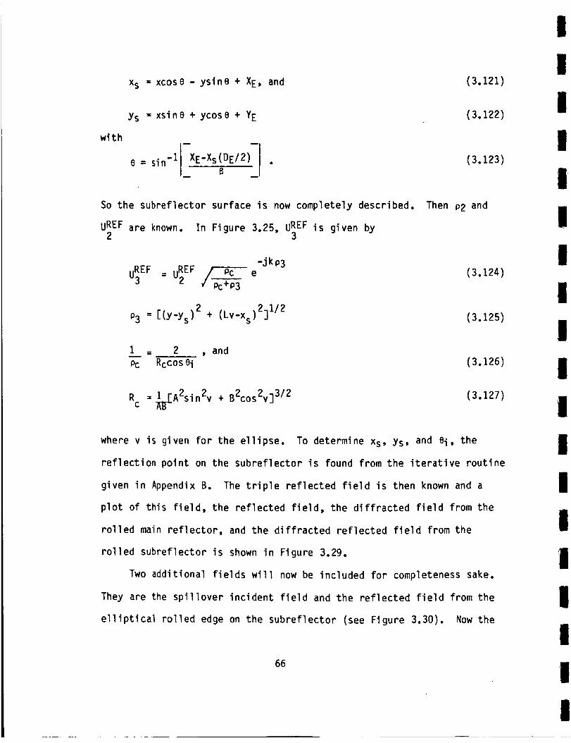
xs = xcose - ysine + XE, and

Ys = xsinO + ycosO + YE

0 = sin-1 E'Xs E/2 •

(3.121)

(3.122)

(3.123)

So the subreflector surface is now completely described.

UREF are known. In Figure 3.25, UREF is given by2 3

Then P2 and

-jkP3

0_ o_/ oce (__Pc+P3

P3 = [(Y'Ys )2 + (LV-Xs)211/2 (3.125)

I = 2 , and

Pc Rccos Oi (3.126)

1 ]3/2Rc = _[A2sin2v + B2cos2v

(3.127)

where v is given for the ellipse. To determine xs, Ys, and 0i, the

reflection point on the subreflector is found from the iterative routine

given in Appendix B. The triple reflected field is then known and a

plot of this field, the reflected field, the diffracted field from the

rolled main reflector, and the diffracted reflected field from the

rolled subreflector is shown in Figure 3.29.

Two additional fields will nowbe included for completeness sake.

They are the spillover incident field and the reflected field from the

elliptical rolled edge on the subreflector (see Figure 3.30). Now the

66

I

I

I

I

|

I

I

I

I

I

I

I

!

iI

I

I

I

I

I

I

I

I

i

III

I

III

i

II

iI

0

_. Fm = I00)_

,,_--: Fc = 80Xr-_ w ,"

_ = 35 °,,.

RCMAIN = I00_,

e_" MAJOR AXIS =5_r_

,',;" MINOR AXIS = 2),.

=1,

' .... 1 .... |" ""' ' | '' " I i .... l" ' "" | .... | ' ' " " | .... I .... l'' ' ' " 1 .... Iz4. 2e. 3z. 36. .o. _.. _e. sa. s6. so. 6_. 6e.DISTANCE FROM CENTER

Figure 3.29 Addition of triple reflected field.

Figure 3.30 Spillover incident field and reflected field.

67

I

I

spillover incident field is simply given by I

-jkPi IUINc = c e (3.128)

with I

Pi = /Y--_'F_ • (3.129) I

The shadow boundary designated by YI may be determined analytically.

The reflected field in Figure 3.31 is given by I

.. -jkPi -jk PrUKLr : c e______ _ e (3.130) I

l

l

I

,_ FC -I i


68

l

I

I

I

I

I

I

I

I

I

t

I

i

I

l

I

l

l

with

1 =1 + 2_ RcCOSoi

and

Rc ")_B:[A2stn2v + B2cos2v]3/2 .

(3.131)

(3.132)

To solve for these variables, the reflection point is found using the

same procedure as that in Appendix B.

Is gi ven by

T .n F .nI

m

n = XoX + yoy

with

T = -x - d; , and

F=x+f_ .

From Figure 3.31 the dot product

(3.133)

(3.134)

(3.135)

(3.136)

Solving for f and d yields

(3.137)

The normal, n, ts given in Appendix B.

f = Asinecosv + Bcos estnv + YE - tAcosvcose - Bslnvsine + YE - s

d = AsinOcosv + Bcosesinv + YEAcosvcose - B'sinvsin'O + XE + Fc-Lv

(3.138)

(3.139)

and

Once the reflection point is known, one finds that

cose I = Bcosvcose - Astnvstne + fEBcosvsine + Astnvcose] ,

[BZcosZv + A2sinZv]l/2[1 + f211/2

69

I

Ioi = [Yr 2+ (Fc'Lv+xr)2] 1/2 , and (3,140)

Pr " [(t'Yr )2 + (LVlXr)211/2 • (3.141) i

IFinally, Figure 3.32 shows the addition of these two additional field

components as well as those already included in Figure 3.29. m

As can be seen from this last figure, it appears that the

Cassegrain system fails miserably when all the major field components I

are included but the last two components examined need not pose any I

concern. First, the feed design itself will include a taper so that the

spillover and single reflected field will be reduced in magnitude. But i

this is trivial because these fields may be eliminated altogether by

_v " 35° I

I_ r " IS"

F m • IOOX I

F "8OXi. MAJOR AXIS B 5Jk

I_ I " SSe MINOR AXIS "2Jk t

I!

I

_,O:'+'_w/'''_e/'" "liJ''*'m;/'*O]Slrl:lNCz'wO/'";;/''FROM'ql/''CENIF.R'S_/'''S_-/ '" "i0/'''6_.''''_;/ I

Figure 3.32 Spillover field and reflected field additions.

70

I

II

Il

I

iI

lIi

I

II

I

!II

ustng a pulse nadar system. In thts system, the length of the pulse

width determines a wfndow through which the return from the target ts

examined. Because the pathlengths of the sptllover field:and stngle

reflected fteld differ greatly from the destred target return, the pulse

radar does not see these returns stnce they are not tn that selective

window. But, the trtple reflected fteld has nearly the same pathlength

as the destred reflected field so thts component can't be overlooked.

The same Is true with the diffracted ftelds, but these are under

relat.lvely good control. So the trtple reflected fteld ts seen to be

the major obstacle to good system performance. Thts fteld wtll now be

examined a little more closely.

Up to this point, the target area or plane of tnterest has been

placed at the focal length. Now ttts advantageous to a!!ow this

distance to vary for added flexfbiltty (see Figure 3,33). The four

field components being examtned must be modified, and thts ts done tn

Appendix C. In Figure 3.34, a representative plot shows the total field

and the total field less the trtple reflected fteld. The trtple

reflected field at grazing Incidence ts not accurately portrayed in thts

ftgure. To increase the accuracy, an additional factor ts included in

the triple reflected fteld expression as follows:

-jcL3/12 -j_/4Rs,h = - _ e e

But for a magnetic line source

-- -I F(X L) +q _,¢L) . (3.142)

71

Din/2 _ .... P

|_

F Fm _ DISPLN

y(T)

Figure 3.33 Target area at variable distance.

DISPLN • Fm

Fm =RCMAIN = IO0)k

_ _v =45°r_ _. 50

r

? _| = 45 °

F=.moX

MAJOR AX1S=2.924_

=' MINOR AXIS =0.855),

=;,0. lO. 20. 30. _O. 50. 60. 70. 80. gO.

DISTRNCE FROM CENTER

Figure 3.34 Total field (_)and total field less triple reflected

field( .... ).

72

(3.143)

_L = -2m(QR)COS 0i (3.144)

XL = 2kLLcos2et (3.145)

LL = srs' (3.146)SC+S i

m(Q) = [kP_(Q)] 113 (3.147)

and pg(Q) ts the radius of curvature of the surface at the reflection

point. This ts already known, sr Is P3, and s' Is -so

LL = P3 " (3.i48)

Note that cose i was calculated before and q* is the Fock integral which

is gtven by

q*(6) = 1 f v'(T) e'J6Tdx7_-=_

with

and

2jv(T)= wi(T) - w2(+)

(3.149)

(3.150)

=-J¢ _t - t3/3wl(t) = 1 / • dt

2 "_ .elj21/3 (3.151)

and c arbitrarily small and positive,

73

Now inserting this factor yields Figure 3.35 as a representative plot.

It is apparent that this increased accuracy shows that the triple

reflected field is a serious problem in the Cassegrain system.

To begin to reduce this field, first consider a Gregorian

subreflector system as shown in Figure 3.36. With this offset design

and the subreflector placed low, the triple reflected field is virtually

eliminated. But this configuration introduces a doubly reflected field

that was not present before and must be considered. First, the normal

reflected field is found (see Figure 3.37). The expression for the

first reflected field is

-jkp i -jk(pc+Pl) j_/2

u_EF = e _e e . (3.152)

The caustic distance Pc may be calculated from geometrical

considerations. So, one obtains that

2 2 1/2Pc = [(Lv+xs) +Ys ] (3.153)

2 2 1/2Pi = [(Fc+Lv+xs) +Ys ] , and (3.154)

2 ]1/2.ym ) (3.155)Pl = [(Ym-Ys)2+(Fm+Lv+xs -

Then UREF is given by2

-jkP2

u_EF = uREF e

with

2P2 = DISPLN + Fm+Lv -ym

(3.156)

(3.157)

74

II

II

i

I

III

III

II

I

II

I

II

I "i'OlSPLN • Fm

Fm,RCMAIN • I00_,

I _ q_v,4S.

_'r" S"

i _5s • 4S"


I

I Figure 3.35 Total field (_) and total field less triple reflectedfield (.... ).

I

l

I

l

I

Figure 3.36 Gregorian subreflector system.

75

III

,, I Iu?, _ '-

I ' _ P I Y, I I

Y'_- x F, "_.._ _L,_..L x' O,SPLN I

' I


since the caustic distance in this case is infinity.

expressed in terms of Ym by noting that

TANa = P2 - DISPLN - Lv = Lv + xs

Ym -Ys

which yields

1 + Lv2 - 2aLvYs = -Lv + a - a (bc) _

with

c = "Lv-xs •

Ys

76

Finally, Ys may be

(3.158)

(3.159)

IIII

II

I

I

II

I

iIi

II

I

il

IIH

Ii

II

I

IiI

Now consider the doubly reflected fteld shown tn Figure 3.38. Agatn,

attach an elliptical rolled edge to the subreflector. The analysis

proceeds as wtth the trtple reflected fteld. The angle eneeds to be

examined more closely tn this situation. If the elltpse ts attached

below or at the math axis (Figure 3.39), then

e = 01 = sin "1[ XE'xs(ATTACH POINT)]B (3.160)

but if it is attached above the matn axts (Figure 3.40), then

e - • - e1 . (3.161)

(ATTACH POINT )

ELLIPSE

Figure 3.38 Doubly reflected field.

77

III

IYs I

...... 8 "-_Xs I

I

Figure 3.39 Attachment of ellipse.

Figure 3.40 Attachment of ellipse.

78

II

II

III

I

II

l

II For a gtven potnt tn the plane of Interest, two reflection potnts

need to be found simultaneously as Illustrated tn Figure 3.41.

l Proceeding as In _opendlx B, the first dot product Is T.

m ;I.FI ;1"T1

I

I

IIF -- I | U: [F

,(xj_p, I

m y, ox +b x_ .ynt)

II

IFigure 3.41

wlth

Doubly reflected field.

- x YRI

nI . _'_ , (3.163)

m _l_+ _JRI2)_;"

m x+ .oo (II

79

I

A A

T1 =x +cy. (3.165)

Solving for e and c yields that

e _-_

CYR1

YR1 - Y(1)

- (Fm+Lv+DISPLN} ]

and

(3.166)

C

YR1 - (Asinecosv + Bcos0sinv = YE

LYRI_ - (Fm+Lv+Acos0cosv - Bsinesinv + XE]

4Fm

(3.167)

The second dot product is

A A

n2"F2 = n2"F1

I_21 ITII (3.168)

with

A A A

n2 = Bcosvcos0 - Asinvsin0 x + BcosvsinO + Asinvcos0 y

LB2cos2v + A_sin2v]_/_ [BZcos2v + AZsinZv] _z

(3.169)

A A

F2 =-x -cy , and (3.170)

A A

2 = -x - ay. (3.171)

Thus, one finds that

a = Acosvsin0 + Bsinvcos0 + YE .

Lv+Fc+Acosvcos0 - Bsinvsin0 + XE

(3.172)

Now the simultaneous solution to the two dot products in Equations

(3.162) and (3.168) is needed to find the reflection point. This is done

80

III

II

II

III

I

III

I

II

I

tterattvely using bisection methods over the v and YR1 intervals until

these values are found within some specified error. Then v and YR1 give

the two reflection points as :"

I

I

I

I

II

XR1 " YR12/(4Fm) (3.173)

XR2 - AcosvcosB - Bstnvslne + XE, and

YR2 = Acosvstne + Bsinvcose + YE •

Then

-jkpl -jkPl

u_EF= • / Pcs ev" _s+Pl

where

(3.174)

(3.175)

(3.176)

II

I

II

Pi = [(Fc+Lv+xR2) 2 + YR22] I/2

Pl = [(Fc+Lv+xR2-XRI) 2 + YRI " YR2)2] I/2

1 1 2

Pcs = Pi + Rccosei

Rc - 1 (A2sin2v + B2cos2v)3/2X_

and cos_ may be found from the second dot product.

reflected field is

(3.177)

(3.178)

(3.179)

(3.18o)

Next the second

-Jk P2. Pcm eI u)_F u_ EF /pc::m + p2

where

1 = 1 + 2m

Ocm Pim Rccos ( _- ei)

(3.181)

(3.182)

81.o

i

i

Pim : Pl + Pcs (3.183) i

Rc = 2Fm + ( ) (3.184) I

cos (_-0i) = -cos 0i (3.185) i

and cosO i may be found from the first dot product. Finally the caustic

distance is

P2 = [(Fm+Lv+DISPLN-YR12/(4Fm)) 2 + (YRI-Y(1))2] I/2 (3.186)

and u_EFD is known. Typical plots for the sum of this doubly reflected

field and the normally reflected field are shown in Figure 3.42. It is

apparent that attaching the edge higher on the subreflector reduces the

field ripple but intuitively this will increase the triple reflected

II

III

field effect which was the original problem. In any case, the effect of

the doubly reflected field with the Gregorian system is unacceptable.

But this system does provide insight into reducing the triple reflected

field by using an offset reflector type of design. So, next let us try

utilizing the offset design with the classical Cassegrain system.

II

IInitially, this type of design poses problems because edges will be

attached to the top and bottom of both reflectors resulting in several

diffracted fields at the junctions. Although the triple reflected field

82

I

m

m iI

I =_=

=

mm

m _°-

I

m _j

m ,4r_

I,

!

m To

m

(a) AttaCh point - O.

A A/ AI

f

A A

M4nor Axis - 0.707REFRM• 5

I ' 1 I

?0, 80. 90.

Attach polnt - S.

h i 45*5"F_m 100F¢•80ATTPT • 5Major Axts • 2Mtnor Axts- 0.707REFRM- $

I ' I | l I ' ' I '

lO. 20. 30, _0. 50. 60. "/0.

DISIANCE FROM CENI[R

(b) Attach point - 5.

"O0_ '' I

gO.

m Figure 3.42 Sum of t,o reflected fields.

I83

mm

.ic_

i .

t

e_l

_0. I0.

Figure 3.42

¢v " 45"

FOrm= S°= 100F¢=80

ATTPT = 10

Major Axis = 2Minor Axts= 0.707REFRM - 2

I ! I I I I I 1

20. 30. _0. 50. 60. 70. 80. 90.


(c) Attach point = 10.

(Continued).

may be reduced, the additional diffracted fields will degrade overall

system performance. If these diffracted fields could be reduced and the

triple reflected field minimized, an acceptable system would be the

result. Through the blending of the edges considered in the next

chapter, diffracted fields are reduced sufficiently to allow the offset

Cassegrain system to work effectively.

84

II

I

II

II

I

lIII

II

II

I

II

I

I

I

I

1

I

I

I

I

I

I

I

I

I

I

I

!

I

CHAPTER IV

THE BLENDED SURFACE

The last chapter brought to view problems encountered in the

Cassegraln system. Now a vlable solution is presented to solve these

problems and obtain satisfactory system performance.

The subreflector edges are the first that will be blended as shown

in Figure 4.1. By a blended surface it is meant that the curved

surfaces are blended between an e11ipse and the original surface to

which these surfaces are attached. As before the hyperbola is described

by

x = a [/1+(y/b) z -1] (4.1)

with

e = sin(Cv+¢r)/2 (4.2)'s'11n{Cv-¢r)l_

a=Fc, and (4,3)

b : a_ . (4.4)

85

i

II

' I

Yi |

IYs

,' |

Figure 4.1 blended surfaces_ I

I

IX E

I

Figure 4.2 Ellipse for upper edge. I

IY(

,A

Figure 4.3 Ellipse for bottom edge.

86

I

I

II

I

I

I

I

I

I

I

I

I

I

I

I

I

I

I

I

I

I

I

The blended upper surface is given tn general by

f - fHYPERBOLAP + fELLIPSE(1-P) (4.5)

P(v) - l+cos(=vlvf) , 0 _ P < 1, and (4.6)Z

v = vf_ t , 0 < v < vf . (4.7)

Note that the parameter through which the blended edge is generated is

Yp with Yi, Yf and vf to be specified, Proceeding as in the previous

chapter, the ellipse to be blended is given parametrically as

X = AsinvcosO - Bcosvsine + XELL (4.e)

Y = Aslnvsine + Bcosvcose + YELL (4.9)

with

0- sin'ICXELL " X(v--O)) . (4.10)B

XEL L and YELL are calculated as in the previous chapter and increasing v

is shown in Figure 4.2. Now Equation (4.5) yields

X(Yp) = X(Yp)HYPERBOLAP(Yp) + X(Yp)ELLIPSE[I-P(Yp)] (4.11)

Y(Yp) - YpP(Yp) + Y(Yp)ELLIPSE[I-P(Yp)] (4.12)

with the blending function P given by Equation (4.6) and v given by

Equation (4,?).

87

The bottom blended surface is generated in a similar manner.

Figure 4.3, v now varies from a specified v_ to _/2. The blending

function is now

l+COS_[ v'vi )P(v) = _/Z-vi

2

with

v = (_- vi)(Yp-Yi_ + vi ,

In

(4.13)

vi _ v < _/2 (4.14)

and Yi and Yf are to be specified.

by

with

The ellipse to be blended is given

X = -AcosvcosO - Bsinvsine + XELL

Y = -Acosvsin 0 + Bsinvcos 0 + YELL

0 = sin-l( XELL - X(v=_/2))B

(4.15)

(4.16)

(4.17)

Again XELL and YELL are calculated as in the previous chapter. The

equations generating this blended surface are then given by

X(Yp) = X(Yp)HYPERBOLA[I-P(yp) ] + X(Yp)ELLIPSEP(Yp) (4.18)

and

Y(Yp) = Yp[I-P(Yp)] + Y(Yp)ELLIPSEP(Yp) (4.19)

Of course between the two blended surfaces the normal subreflector is

described by Equation (4.1).

Now the centers of the ellipses will be given. The normal to the

hyperbola is given by Equation (3.117) and evaluated at Yi for the top

88

III

I

II

I

III

II

II

II

I

I

edge, Then, one finds that

M M M M M

XELL X + YELL Y " X(Yi)X + Yt Y + Bn

A

and for the bottom edge with n evaluated at,Yf ts specified by

M _ M A

XELL X + YELL Y " X(Yf)X + Yfy + Bn

(4.20)

(4.2z)

I

iII

II

II

I

III

Now the offset subreflector with two blended surfaces Is completely

specified by Equations (4.18), (4.19), (4.11), (4.12), and (4.1). The

parameters that can be varied are YI and Yf for the top and bottom, vi,

vf, and the major and minor axes of both ellipses.

The design of the surfaces may proceed and a few general rules are

given here to simplify the procedure. It is convenient to use the same

values for the axes of both ellipses and fix vi at -_/2 and vf at _.

This allows the knife surfaces to be completely removed from view of the

source. The excessive hidden surfaces on the subreflector, as well as

the main reflector later on, are removed by limiting the range over

which the curve Is generated. This is In general better than

respecifying vi and vf which would lead to surfaces whose shape Is

changed each time. In general, the larger the surfaces, the flatter the

field will be. But small surfaces are also desirable to taper this

field to reduce the effect of the triple reflected field. So a tradeoff

exists in the size of the surfaces . This slze is determined by the

major axis of the ellipse as well as the length of the blended hyperbola

section (which Is determined by Yi and Yf). Now the minimum radius of

curvature of the edge must be kept greater than a quarter wavelength at

89

the lowest frequency of operation. Once the general size of the

surfaces is decided, the radius of curvature is determined by the minor

axis dimension of the ellipse. One final constraint is the relationship

between the major axis length and the length of the hyperbola section.

By looking at the slope or first derivative of this curve, a gradual

transition is best obtained for a hyperbola section length that is

approximately four times the major axis length. Again, this constraint

is true at vi equal to -7/2 and vf equal to 7. So when designing the

surfaces , the size for acceptable performance is the overriding

consideration. Besides the design of the surfaces, the size of the

subreflector itself is another variable. It must be large enough to

illuminate satisfactorily the main reflector yet kept as small as

possible so that interactions between the two reflectors may be

mini mi zed.

The field produced by the subreflector will now be examined. Using

UTD and physical optics, the field along a parabolic contour is

calculated. Using a magnetic line source (Figure 4.4), one finds that

the reflected field is given by

-jkPi -jkPruREF = e _e . (4.22)

_pc_r

For the region between Yi add Yf, UREF has been calculated before with

Pc = [(Lv-x) 2 + Y2] I/2 (4.23)

Pi = [y2 + (Fc-Lv+x)2]I/2 (4.24)

Pr = [(yp.y)2 + (Fm_Lv+x_yp2/(4Fm))2] I/2

90

(4.25)

I

II

II

I

III

III

I

II

II

II

I

I

I

I

I

I

I

I

I

I

I

I

I

I

I

I

I

I

I

Figure 4.4 Field a]ong a parabolic contour.

91

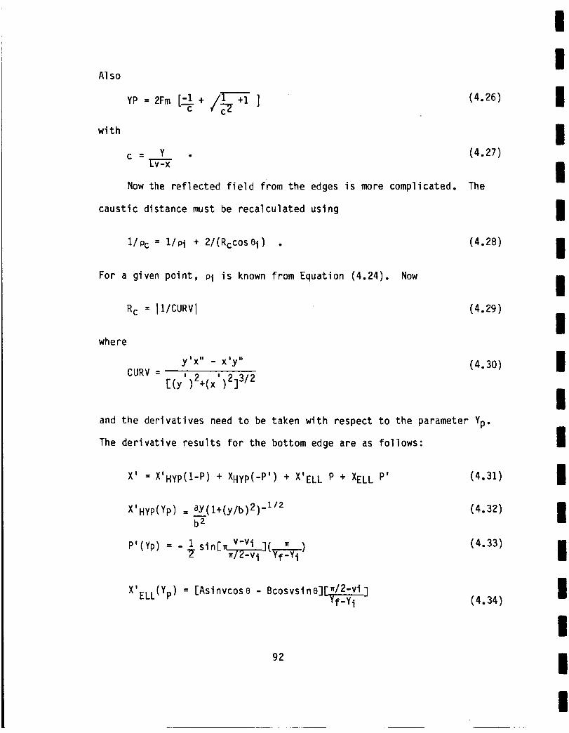
A1 so

with

YP = 2Fm [-1+ /____+1 ](4.26)

c = Y • (4.27)

Now the reflected field from the edges is more complicated. The

caustic distance must be recalculated using

1/p c = 1/pi + 2/(RccosOi) . (4.28)

For a given point, Pi is known from Equation (4.24). Now

Rc = I1/CURVl (4.29)

where

CURV =y'x" - x'y" (4.30)! !

[(y )2+(x )2]3/2

and the derivatives need to be taken with respect to the parameter Yp.

The derivative results for the bottom edge are as follows:

X' = X'Hyp(I-P ) + XHyp(-P' ) + X'ELL P + XEL L P'

X'Hyp(Yp) = aY(l+(y/b)2) -1/2

b2

- SlnET ' ](_)P'(Yp) = } " v-v i_/Z'vi Yf-Yi

(4.31)

(4.32)

(4.33)

X'ELL(Y P) = [AsinvcosO - BcosvsinO][_/2-vi]_f-Yi (4.34)

92

I

iI

II

I

II

III

I

II

II

II

U |

X" - XHyp(Z-P ) + 2 XHyP (-P') + XHyp(-P")

II I

+ XELL P + 2 XELL P' + XELL P"

N

XHyp(Yp) , a/b 2

(4.35)

(4.36)

(4.37)

It

|

Y' =(l-P) +Yp(-P') + YELL p + YELL P'

(4.38)

(4.39)

r -iYELL(Yp) - (Acosvsine + Bcosvcose)

Y" = -2P" + Yp(-P") + Y_LLP + 2Y_LLP' + YELLP" , and

(4.40)

(4.41)

U

YELL(Yp) = (Acosvsine- Bsinvcose)l-l/2"vt-] 2

The derivative results for the top edge are as follows:

(4.42)

I !

X' - + XHypP' ÷ Z-P) + )XHypP XELL( XELL(-P'(4.43)

P'(Yp) =-½ S]N[_.fV](_-_t) (4.44)

XELL(Yp) = (AcosvcosB + Bstnvstne)( )

93

(4.45)

II I U I

X" = + 2XHypP' + + l-P) + (-P'XHypP XHypP" XELL( 2XEL L ) + XELL(-P°')

(4.46)

" ] IXELL(Yp) = (-AsinvcosO + BcosvsinO) --vf --2 I(4.48)

I(4.49)

I

(4.50) m(4.51) m

!

y, = p + YpP" + YELL(I-P) + YELL(-P')

YELL(Yp) = (Acosvsine - Bsinvcose) --vf --

I0 I

Y" = 2P' + YpP" + YELL(I-P) + 2YELL(-P' ) + YELL(-P"), and

YELL(Yp) = (-Asinvcose + Bcosvcose) --vf --2

These derivatives provide the information necessary to compute the

(4.52)

radius of curvature. The normal is computed next so that cose i may be

found. For both edges the slope is given by

I

II

m = Y'IX' (4.53)

and the normal has slope -1/m. For both edges the normal is given by

/ - /n = Xnx + Yn = -x + (l/m) . m

[1+1/m2] "/z (4.54)

Now forming the dot product with the incident vector, one finds that

94

A M

-(Fc-Lv+x)x-Yy

[ {FC-L_X}_+Y_JZ'_Z

which .yi el ds

(4.ss)

cose i ,, -Xn(Fc-Lv+X)-YnVL'(Fc-LV+X) _+y ;:ji iz (4.56)

I

II

II

III

I

III

I

Note that the caustic distance Pc is known. Equating the angle of

incidence with the angle of reflection al]ows the point YP on the

parabola to be found. So one obtains that

A

PP = -{Fm'Lv+X'yp2/{4Fm));+(YP'Y_[(Fm.L_+X.ypz/(4Fm_)Z_(yp.y)z /z

and

(4.57)

cos ei = -Xn (Fm-Lv+X- (YP)21(4Fm) )+Yn (YP'Y)

[(Fm-Lv+X-YP 2/(4Fm) )2+(yp.y) z] zIz . (4.58)

Using an iterative bisection method, YP may be found numerically. Then

the reflected field from the blended surfaces along a parabolic contour

is known. Numerically, it is convenient to pick points on the

subreflector and ray trace to the corresponding point on the parabolic

cu rye.

The subreflector is now analyzed using the physics optics

approximation and the results compared with the reflected field given by

geometrical optics. Again using a magnetic line source, the current on

the lit side of the subreflector is given by

m A

as = Znx Hi . (4.S9)

95

I

In Figure 4.5, _i is z-directed and the normal n lies in the x,y-plane.

The two dimensional radiation integral is used to compute the

subreflector scattered field which is given by

j_14 .... jkp A ^

Hz = _ e f z • (t x P)Jt e (Pi-n)dJ_ (4.60)

where

and

I

I

II

_zZ"'°__ I;.i:H :e _ (4.61)V_T

Js = JtC : 2H_t . (4.62)

The slope (m) is given by Equation (4.53) and the unit tangent by

^ A A= tx + tyy = x+my for m positive (4.63)

¢_+-_m

= + = -x-my for m negative or

VI+m-_-_L_- m positive on lower edge. (4.64)

Also, one finds that

Pi = [y2 + (Fc_Lv+X)2]I/2 (4.65)

and Jt is then known. Now, one obtains the following:

II

II

p = [(Fm-Lv+X-(YPAR)2/(4Fm))2 + (YPAR-y)2] 1/2 (4.66)

A A 2 ^

P = Pxx + PyY = -(Fm-Lv+X-(YPAR) /(4Fm))x + (YPAR-Y)y

p (4.677

96 o

II

I

j SOURCE

L r I "" " -

m Figure 4,5 Physical optics analysis,

I

I

m

I

II

III

Figure 4.6 Three integration regions.

97

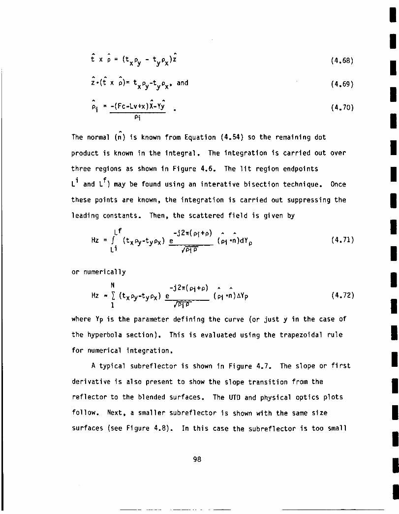
6 x _= (txpy- typx)_

_-(6x _)-txpy-typx,and

^ )_yyPi = -(Fc-Lv+x - .

Pi

The normal (n) is known from Equation (4.54) so the remaining dot

product is known in the integral. The integration is carried out over

three regions as shown in Figure 4.6. The lit region endpoints

Li and Lf) may be found using an interative bisection technique. Once

these points are known, the integration is carried out suppressing the

leading constants. Then, the scattered field is given by

Lf -j2_(pi+p) A ^

Hz : f (txPy-tyPx) e (Pi ,n)dYp

Li _Pi_

(4.68)

(4.69)

(4.70)

(4.71)

or numerically

N -j2_(pi+p) ^ ^

Hz - Z (txPy-tyPx) e (Pi .n)aYpI

where Yp is the parameter defining the curve (or just y in the case of

the hyperbola section). This is evaluated using the trapezoidal rule

for numerical integration.

A typical subreflector is shown in Figure 4.7. The slope or first

derivative is also present to show the slope transition from the

reflector to the blended surfaces. The UTD and physical optics plots

follow. Next, a smaller subreflector is shown with the same size

surfaces (see Figure 4.8). In this case the subreflector is too small

(4.72)

98

III

I

II

II

III

II

II

I

II

I

% " 45° i"m _ . 5oFm- 81.33 _,Fc - 81.33X

m Major Axts - 2.67xMinor Axis - 1.73x _'Hyperbola Section - 10.67XEdges attached _"

m at 4.12x and 6.543x

Tm .-

! ,

! -TII. 7S. TI. 11. lg.

(a) Subreflector with biended edges,

, i'!

m _,-1

" //m ..

"/m -• "_ .... ' '"i"";"'i'i' .... "

", ,_ ' ..... , /,:T-COOROINRTZ

l (b) First derivative plot.

Figure 4.7 Subreflector with blended surfaces,

99

1,o

mD

?

%:

Figure 4.7

"";o: ..... ""u'" "/ ,o. ,o. ,o. ,o. ,o ,/ DISTflNCE FROM CENTER

(c) Geometrical optics plot.

°.o

mm

e

°.

?

DISIRNCE FROM CENTER

(d) Physical optics plot.

(Continued).

100

II

II

I

III

II

II

II

II

I

I

(_V = 45o_r = 50Fm = 81.33 XFc = 81.333,Major Axis = 2.673,Minor Axis = 1.73),Hyperbola section = 10.67XEdges attached

at 5X abd 5.5),

=t

|

7_. 75, 76. 77. ; .

(a) Subreflector with blended surfaces.

D

o,411

==" / I

-,."'£" ,.'-iJ r i: ';J ,Y ;."1;.' -i J-i J/,;" ,'i;_/'r- cooBoI NA|E I

(b) First derivative plot.

Figure 4.8 Smaller subreflector with same size surfaces.

i01

..

• "_o] "DISTANCE FBOM CENTEB


Figure 4.8

0

l

",0; • ' ' _o] ' ' "_o: " ' " ;o_ " ' ' _o_" " " _o] ' " ' _o_" ' ' Go:' ' ",o_DISTANCE FBOM (ENTEB


(Continued).

102

IIIII

II'!

!!!!

!I

!I

!

in terms of wavelengths. Finally the original size subreflector with

smaller surfaces is considered (see Figure 4.9). Again, performance

suffers and the slope transition in this last figure is much more

abrupt.

It is also helpful and convenient to look at the far field of the

subreflector using geometrical optics (GO) and moment method theory.

For GO, the far field is given by

-jkPi -jkPs

U = e _ e (4.73)

_/'_" V pc+Ps

with the variables shown in Figure 4.10. Now Ps is the far field

distance so

Pc+p$ _ Ps , and (4.74)

-jkp i -jkp s

U =e p_c e (4.75)

But this last factor is a common factor and may be ignored yielding

(4.76)

at a specified angle ¢ which may be easily found from previous

calculations.

For the moment method, points are set up along the curve of the

subreflector a distance "ds" apart. The distance used was usually about

0.2 wavelengths at a particular frequency. On the blended surfaces,

"ds" was approximated as a small line segment. For the hyperbola

section (Figure 4.11), the uniform segments were found using

103

I

III

_v " 450Cr " 50 IFm = 81.33 ),Fc = 81.33 ),Major Axis = 2.67), IMinor Axis = 0.433),Hyperbola section = 2.67),Edges attached at []

4.121 and 6.543),

Iii iei"ege .(a) Subrefle o n d

Ii

I

[]

(b) First derivative plot. I

Figure 4.9 Origtnal subreflector with smaller blended surfaces.

104

Figure 4.9

>i ,o' 20' ,o' ,o' " ';o]''';o]' "';o. "" ";o.DISTRNCE FROM CENTER


o

m

4

T

.... I .... I



(Continued).

105

I

i

Figure 4.10 Far field from subreflector.

ID_

I

' |

dx

Dx d--_

Dy _s ( _÷ (j__y)-dx 2

Figure 4.11 Moment method geometry.

106

I

I

!

iII

IIIII!!

I

i|,,

i/

dx = ay/b 2

_]_ [1+(y/b)2] I/2 (4.77)

at the bottom point and

dy = ds (4.78)

[l+(dx/dy)2] I/2 •

This dy is added to the previous y to obtain the next y from which the

corresponding x coordinate may be calculated. Once the subreflector is

represented by the point geometry spaced ds apart, the moment method

program may be run using this information to obtain far field plots.

Using the same subreflector geometries as in Figures 4.7 through 4.9,

GO and moment method far Field patterns are shown in Figures 4.12

through 4.14. The moment method analysis provides accurate results and

for the relatively small subreflector is easily and quickly implemented.

These results also show the closeness of including only the reflected

field in the UTD analysis. When these two procedures yield results that

differ greatly, then more than the reflected field is being seen, and

the design must be compensated so that it looks more like a simple

reflective surface. Once satisfactory performance (flat amplitude over

area of main reflector to be illuminated) is obtained, the design of the

main reflector may proceed.

As with the subreflector, the main reflector will consist of a

parabolic surface with two blended surfaces attached (Figure 4.15). Of

course, the parabolic section is given by

x = y2/(4Fm). (4.79)

107

I

I

:___ ___ 1 _

I!̧•11!I!.-.ILl [i-_ 7_'i" "i. i-_"i_ ............

m,zs. i)o. m. ,.o. I,s. iso. ,$s. ,,o. " " "m. •

ANGLE IDEGREES) IN

(a) Geometrical optics plot for geometry of Figure 4.7 (a). I

I

i_o. izs. I)o. in. lu. iis. iso. iss. iso. iss. I

ANGLE IOEGREESI

(b) Moment method plot for geometry of Figure 4.7 (a). I

Figure 4.12 Field plots for geometry of Figure 4.7 (a). i

108

.........................., ....... • .... "_"]'.-_'_ "1_-_11.'i

I--EIT-TZ__.ZI /;J- 'N'N.. i,.ii_ _i_ i;iIi

" !"-:::t:Til::/, :: 1 : }: l:i!il:• '7_ __-2_.7 /12,21:i ?2 .... i -.l::'N 7:? :

- .

,o._ . ........ 22 " ''2"i "112

I_0" I_S. II0. IIS. lliO. llS. lliO.

ANGLE (DEGREESI

\I||. I10. IIS.

(a) Geometrical optics plot for geometry of Figure 4.8 (a).

\

II

ISS.IZS. ilO. I1|. lliO. Iql$. 114). liO. IlS.

ANGLE IDEGREES!

(b) Moment method plot for geometry of Figure 4.8 (a).

Figure 4.13 Field plots for geometry of Figure 4.8 (a).

109

+i÷i-i

"i__!_J -_il!i:i;iiiiSII11]iii°r

o ', .....

I_/ili. I_. llO. llS. llO. IllS. Illi_. lllili. IllO. lll$oANGLE IOEGREES)

(a) Geometrical optics plot for geometry of Figure 4.9 (a).

i:: . ; T . " . . T

'..i I _i/

o,',

,,1;.t_]_ .._ .... !I liIJ, IN, IllS, llllO, IllS, liO. IllS. I$0. IllS.

ANGLE ID[GREES!

(b) Moment method plot for geometry of Figure 4.9 (a).

Figure 4.14 Field plots for geometry of Figure 4.9 (a).

110

!

!

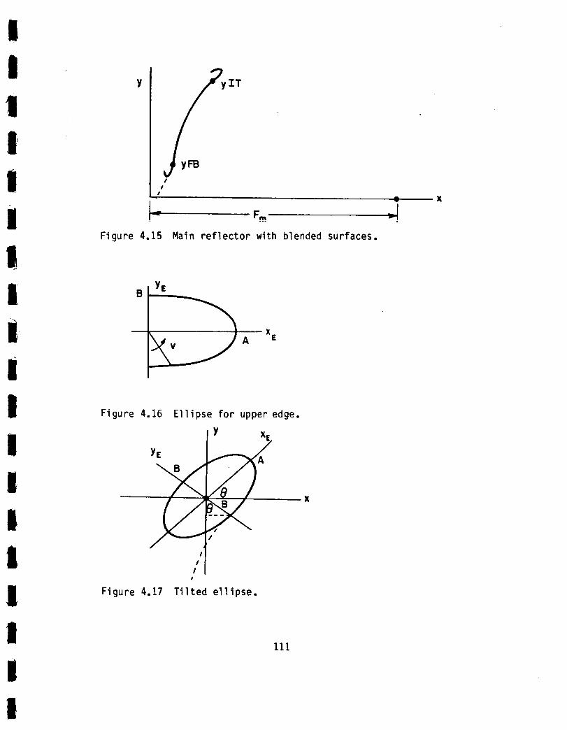
t yy_'T

!Ii|

Figure 4.15 Main reflector with blended surfaces.

I

!

I Figure 4.16 Ellipse for upper edge.

I

I

I#

Figure 4.17 Tilted ellipse.

X

111

"7

!

!XE

!

I

Figure 4.18 Ellipse for bottom edge.

The blending function used on the top edge is

cos {p = I+ 0 < P < 1 (4.80)

2

where

v = vf_ 0 • v • vf . (4.81)

The ellipse in Figure (4.16) is parameterized by

XE = Asinv, and (4.82)

YE = -Bcosv . (4.83)

The normal of the parabola is given by

A ^ A

n = -x+(Y/2Fm) y

[I+(Y/2Fm)_] ii_

(4.84)

112

a

|

IIiiIiiII

Ii

so the origin of the blended ellipse is located at

= -B + YIT2

XELT [I+CYIT/_] ip_ E , and

B(YIT)F-_

YELT = [1._ (_I._l)z]L/_lPm

+ YIT.

The angle of the main axis of the ellipse is now tilted (Figure 4.17)

and given by

e = sire-1 [YIT2/(4FM)'XELT]

B

so that the elliptical curve is generated by

and

X = Asinvcose + Bcosvsine+XEL T

Y = Asinvsine - Bcosvcose + YELT •

Finally the top blended surface is generated by

and

X = (_m2)P + (Asinvcose + BcosvsinB + XELT)(1-P)

Y = YpP + (Asinvsine - Bcosvcose + YELT)(I-P)

where Yp is a parameter that varies between YIT and YFT.

(4.85)

(4.86)

(4.87)

(4.88)

(4.89)

(4.90)

(4.91)

For the bottom surface, the ellipse (Figure 4.18) is parameterized

by

XE = -Acosv (4.92)

113

I

and

YE = -Bsinv (4.93)

The origin of the ellipse in this case is at

lII

and

: -B + YFB 2

XELB I+(YFB _ ii_[ ,Tlr_,]

(4.94)

i

iI

B(YFB) (4.95) I_m + YFBYELB = [1+ YFB z i,_

The tilt angle of the ellipse is

0 = sin "I [YFB2/(4Fm)-XELB]B

(4.96)I

Iand the ellipse curve is given by

(4.97)

(4.98)

i

(4.99)

. (4.1oo)

I

X = -AcosvcosB + BsinvsinB + XEL B . and

Y = -Acosvsine - BsinvcosB + YELB •

The blending function for this surface is

v-vi- lP = 1+cos_ _/2-v iJ O<P<I

with

2

v i < v < 7/2v (,/2 vi ),Yp-YIB ,= - [YFB-YIB ]+vi

Then the bottom blended edge is generated by

114

and

X : (yp2)4Tm (1-P)+(-Acosvcos0 + Bsinvsine + XELB)P (4.101)

Y = Yp(1-P) + (-Acosvsine- Bsinvcose + YELB)P . (4.102)

The entire main reflector surface may now be generated. As in the

case of the subreflector, larger surfaces lead to flatter field

performance. This overall size is determined by the major axis length

plus the parabolic section length blended together. The parabolic

section length is determined by (YIT,YFT) and (YIB,YFB) for the top and

bottom surfaces , respectively. The minimum radius of curvature of the

surface is determined by the minor axis dimension, and this is kept

greater than a quarter of wavelength at the lowest frequency of

operation. A final rule of thumb is to make the length of the parabolic

section about four times longer than the major axis of the ellipse in

order to make the slope transition from the parabola to the blended

surface as gradual as possible. As in the subreflector case, vi is

fixed at -_/2, and vf is fixed at 7. This assures that the surface

extends well into the back area of the reflector. Since much of this

blended surface is excessive, some of it may be eliminated by

controlling the range over which the total reflector is generated. This

is easier to implement than changing the variables which govern the

shape of the curve which would result in a different surface design.

With the geometry given, the field in the plane of interest or

target area may now be calculated. The main reflector is analyzed alone

115

by placing the source at the virtual feed. The momentmethod procedure

and GOare used to analyze the main reflector. First, the momentmethod

is used to consider somespecial cases.

In Figure 4.19, a typical reflector with sharp edges is shown. The

momentmethodplot follows. The ripple maybe greatly reduced by

attaching elliptic rolled surfaces with no blending involved as in

Figure 4.20. Nowusing a linear blending function of the form v/vf

instead of the cosine function described earlier, the field plot in

Figure 4.21 showseven more improvement. A parabolic blending function

of the form (v/vf) 2 is considered next. The improvement of the field in

this case is shownin Figure 4.22. Finally, the original cosine

blending function is used as shownin Figure 4.23. It and the parabolic

blending showsimilar results. The cosine blending is chosen since it

gives the best results and also does a good job of shaping the surfaces

in the back region. The distance to the target area or plane of

interest is also a variable, and care must be taken in choosing this

distance. If the observation plane is too close to the reflector, one

is limited by the feed position. If the plane is movedtoo far away

from the reflector, far field effects becomeapparent, and the plane

wave gradually becomesmore and more tapered. These effects are shown

in Figure 4.24 for various observation plane distances where "DISPLN"is

referenced to zero at the virtual feed. The case for DISPLN= 0 is

shown already in Figure 4.23b.

116

iiil

!

1!!I!

I

ilIII

IIiIi

IDS:

O?.

+i _i_o

1,

"i" •

@:'" i,;.i

Figure 4.1g

/-' /

//

z,S /

- /8

_: /

©-.

,i/

CM

CV = 45°

Cr - S°

Fm = 610 cm

Top at 505 cmBottom at 322 cm

{a) Parabolic reflector section.

f - ' .._ V

,_,_____. 1. • - .... :

" I + -..!- +_+!_ , !!:j

i: -¸

Ui_h|If

IlO'l. II1_. qlIS. SILO. '11_1. I?ql. 111/7. gig0.

DlSll_NCtr FAOM AXIS [CMI

(b) Moment method plot.

Parabolic reflector section and field plot.

117

I

Figure 4.20

!

I

I

. ! |I

+,_ / ,v,,o I,-._ / +I-'5 ° i

/ Fm - 610cm •/ Top at 505 cm

Im

_ / Bottom at 322 cm

_/ / Majhor Axis = 80 cm i

+++++ m

(a) Reflector with elliptic rolled edges, m

IIi_: _. Me. sot. NZ. _J$. We. R_. S_. UT. _. II

OI$TRN_ FRO. AXIS (CH)

(b) Moment method plot. Frequency = 4 GHz

Reflector with elliptic rolled surfaces and field plot. I

11B

lI

I

; =

(a) Linearly blended edges.

I 'l_1..I_.!.,J_J ! _ _ _ll ",t_:I_: I:__/i I..--T_ __ .1

_1.:-I. lr: ]_'iI I _I_ _ : _ I: '1"t :!1"?I /'1_:'1" 1"" I'_: \:! _'1 I

l

t

(b) Moment method plot, Frequency - 4 GHz

Figure 4.21 Reflector with linearly blended surfaces and field plot.

11g

I

Figure 4.22

!I

_v " 4S°¢r " 5oFm = 610 cm


Major Axis = 80 cmMinor Axis = 30 cm

Parabol ic Secti onblended = 320 cm

I

!

I_. _Z. 8114. MS. N_. QIS. ISl. ll_l • S11. _?. UO.OISTANC[ FMO. Rxls tc.J

(b) Moment method plot. Frequency = 4 GHz

I

II

II

!

!Reflector with parabolic blended surfaces and field plot.

I

I120 I

I

t

°

tl:v _

f

45 °5°

Fm ,, 610 cmTop at 505 cmBottom at 322 cm

Major Axis - cm80Minor Axts - 30 cm

Parabolic sectton

i blended • 320 cm

). ' ', uI_I. q*?. II. III. IIIII.

C_

I ,..

i !:

#.

*T

Ii L

I

(a) Cosine blended ed9es.

:.::-lii " iI_ _ :1 :;1_z..i l--

-i_i!iV.l/1!._ : :! !i.t;:,!il\-_-.il:i!:li-]

;i_X::l ii :1!.-_i_ii-I-;t-;;;l:_iit,!Xl: il

I_I0. loll. _$II. lOS. INI_. III$. lllll. IIII. II?II. II?. lill_.OJSTRNC lr IrfiOH RX]$ |CPtJ

(b) Homent method plot. Frequency • 4 GHz

Ftgure 4.23 Reflector wtth cosine blended surfaces and field plot.

I

I121

I

The GO reflected field for the main reflector will now be

calculated (see Figure 4.25). In the parabolic region, the reflected

field is given by

-jk (Pi+Pr)

uREF = e (4.103)

with

Pi = [(Fm-X)2+y2]I/2 • (4.104)

Pr = Fm + DISPLN-X, and (4.105)

YPLN = Y . (4.106)

For the top and bottom blended surfaces, the reflected field is

-jk Pi -jkPruREF = e _ e

T /p_Tp_(4.107)

with

I =1 + 2

p--c p_- Rccos 0i (4.108)

and Pi as before. To calcualte Rc and cosOi, the partial derivatives

with respect to Yp must be found. For the bottom surface, one finds the

fol lowi ng:

I I

X I o= XpARA(1-P ) + XpARA(-P' ) + XELLP + XELLP (4.109)

122

liIi!

I

IiI

o_ .... • +. ++ _ _ + i + , ! .4 • I .... J+ :-+ +4 ...... J . . +

i • •_m . J -++ . • T • " ; : I 2 _ ...........

i (+:I HI • _PS$ . 1011. 312. I I S. III. I;) I • 1711 . 127. II0

DISTFINCE FROM RXI5 ICN)

(a) DISPLN = -305cm.

I

(b) DISPLN = 305cm.

Figure 4.24 Moment method plots for various distances to the

observation plane.

123

I!

'_i__!!-_t_.!_fl_-_ __:1_:t-_ _i!_t _--I ' _ II

.," I

I !0_1. lSS. lOlL 1162. IllS. ql$i. S21 . S?ll, 127. leO. iDISTANCE FROM AXiS (CN) •

e

(c) DISPLN : 610cm.

!

#

Figure 4.24

I?!iil

_!_i¸!;_-__ _ _ _ I_!!-- It ,!-!!i_!!-_!!:._i_.! !_i _:.:_::_:_-_:::i!,.::. : _: i... .... i ......

a?O$. _S$. loll. IIS_. IllS. 1158. S:ll • S?l. i;_7. OIO.DISTI::INCE FROM HXIS (CM)

(d) DISPLN = 1220cm.

(Continued).

124

!

I

ilIII

IyFB

Figure 4.25

ylTn

Pr

Pi

Fm _l_ DISPN

Reflected field from main reflector.

125

Lw yPLN

XpARA(YP) =

, . 1 sin[It( v'vi _]r _ 'P (YP) = 2" _-vi j _YFB-YIB J

I

XELL(Yp) = [Asinvcose + BcosvsinO]( _/2-vi"YFB-YIB"

II n I

X = XpARA(I-P ) + 2XpARA(-P' ) + XpARA(-P" )

II I

+ XELLP + 2XELLP + XELLP"

I!

XpARA (Yp) = 1

P"(Yp) = ½cos

(4.110)

(4.111)

(4.112)

(4.113)

I

(4.114) I

I(4.115)

I-- --I2II _J --IP) ,,.iis s'- ,

^ELL L_COSVCOS(_ - BsinvsinBJ YFB-YIB

I

Y' = (l-P) + Yp(-P') + YELLP + YELL P'

!

YELL(Yp) = (Asinvsine - BcosvcosO)( _/2"vi"YFB-YIB"

126

(4.116)

(4.117)

(4.118)

I

II

i!

II

I

II I

y" = -2P' + YP(-P") + YELLP + 2YELL P' + YELLP" '

Y_LL(yp) = [Acosvsine + Bsinvc°sO]I-_/2"vi _I 2.

For the top surface, one obtains the following:

X' ' + ' + ' l-P) += XpARA P XpARA P XELL( XELL (-P')

p, = .I_.sin _v

X_LL = (Acosvcose - Bsinvsine)(y-_i _)

:I X" = X_ARA P + 2XpARA P' + XpARA P"

I + X_LL(1-P) + 2X_LL('P' ) + XELL('P")

I -- _ --2

I X_LL(yp) = (Asinvcose _ VcosvsinB)

I

1I

i

y, = P + YpP' + Y_LL(1-P) + YELL(-P')

, y__YELL(yp) = (Acosvsine + Bsinvc°sO)(

127

and(4.119)

(4.12o)

(4.t21)

(4.122)

(4.t2_)

(4.124)

(4.125)

(4.126)

(4.127)

(4.128)

i

I I

Y" = 2P' + YpP" + Y_LL(1-P) + 2YELL(-P ) + YELL(-P") , and(4.129)

Y_LL = (-AsinvsinB + Bcosvcos0)[_) 2 . (4.130)

From elementary calculus,

A

F = xx +yy

with

the position vector is given by

(4.131)

F :x'x+ y_, and (4.132)

IF, I = [(x,)2 + (y,)211/2 . (4.133)

Also, the unit vector is

^ F' x'x + y'y

t = I-_- [(y,)Z+(y,)Z]i/z (4.134)

and

t,:x[x"-x'(x'x"+y'y")[(x')2+(y')2] -1]+;[y''-y'(x'x''+'_y")[(x')2+(y')2]'l]

[(x')2+(y,)_] I/2

(4.135)

i i J1o I Ij s

D

_: t' . (4.136)

IF'l

The radius of curvature is given by

R : 1

c I_--F (4.137)

128

,

I

IIII

I

iII

I

I

and the outward facing normal by

A

n _ •

The dot product with the incident vector

Pi = (Fm-x

[(Fm-x) _+yZ] _/z

(4.138)

(4.139)

m I. .....

lll_iJ 6101:11 bll_ i UI llI_:_U _I_IUlII_

A A

cosO i = pi'n (4.140)

and the caustic distance Pc is known•

The reflected field is solved completely when YPLN and Pr are

known. First, one obtains that

Pr = [(Fm + DISPLN - x) 2 + (YPLN - y)2]I/2 . (4.141)

For the bottom edge (see Figure 4.26), one finds that

aI = TAN-I((Fm_x)/y)

and

(4.142)

= c°s-l(c°s°i ) • (4.143)

The normal is always outward facing so if a2 > _/2 then subtract a2 from

to get desired a2. Then, one obtains that

TAN(al+2a2) = (Fm + DISPN - x)/(y-YPLN) (4.144)

or

129

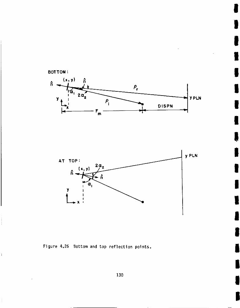
BOTTOM :

A^ (_" Y) n

Y PiL',DISPN

ira= YPL.N

AT TOP: _ yPLN I

I 'y , |

I I

Figure 4.26 Bottom and top reflection points.

130

III

IlII

If

III

ilil

!

YPLN = -(Fm + DISPN - x)/TAN(a I + 2a2) + y . (4.145)

Similarly for the top surface, one obtains that

TAN(_ 1 + 2a2 - _/2) = (YPLN - y)/(Fm + DISPN - x)

or

(4.146)

YPLN = (Fm + DISPN - x) TAN(a I + 2a2 - _/2) + y . (4.147)

The reflected field for the surfaces is then given by Equation (4.107).

In Figure 4.27, a typical main reflector is shown. The slope or

first derivative is also present to show the slope transition from the

reflector to the blended surfaces. The GO and moment method plots

follow. Next, smaller surfaces are attached (Figure 4.28) and the

degradation in the field is apparent. The GO plot is not as greatly

affected since it only contains the reflected field components. Larger

surfaces will result in flatter field performance, but a tradeoff must

be made between edge size and field performance. Once the field is

acceptable, the surfaces should not be increased further in order to

keep the triple reflected field to a minimum.

The total system may now be put together. The subreflector and

main reflector have been analyzed separately, and there is little

further design that can be done at this stage. The offset between the

reflectors should be as large as possible, and the blended surfaces have

been made as small as possible to reduce the triple reflected field

without sacrificing flat field performance.

131

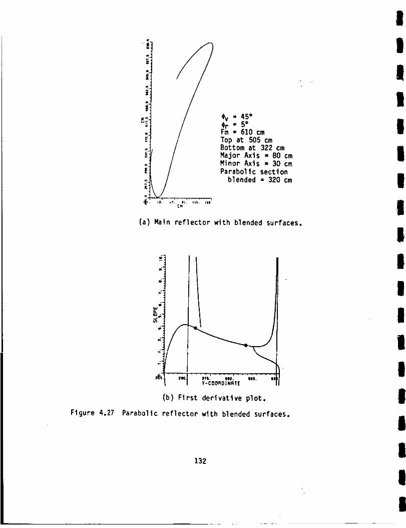
Figure 4.27

=_

P

jJ;/

///!

_*" v .... i .... = .... u

13. ,7. al. I1$. 119,

EM

+V = 450Cr = 50Fm = 610 cmTop at 505 cmBottom at 322 cm

Major Axis = 80 cmMinor Axis - 30 cm

Parabolic section

blended = 320 cm

(a) Main reflector with blended surfaces.

0w

o,e-

o.g

bJ

O.

/

T-COORDINRT[


Parabolic reflector with blended surfaces.

132

II

II

I

I

II

III

I

III

lI

I

I

I

i

I

I

II

iI

Ii

i

i

i

II

I

iiiliiiilli/ "'i-- : ;7 " "" _ " "

i

r

.-? .............. t

--In

I

L:_. - J - 4.-._-. . ; .......

: ; _-':_- ::::::1 "_ ....../ /

I I

l

$09. ,$2, qlS. qlO. S21. _ S?q, 627. I80.

DISTRNCE FROM AXIS (CH)

(c) Geometrical optics plot. Frequency = 4 GHz

°,

,, i_i ,

20,.

,.....;i

!-. - 1_!ili!_.."o

.... ! ....2Si. 309. ,62. qlS. q68. S21 • ill. I!1. llO.

DISTANCE FROM RXIS (CM)

(d) Moment method plot. Frequency = 4 GHZ


133

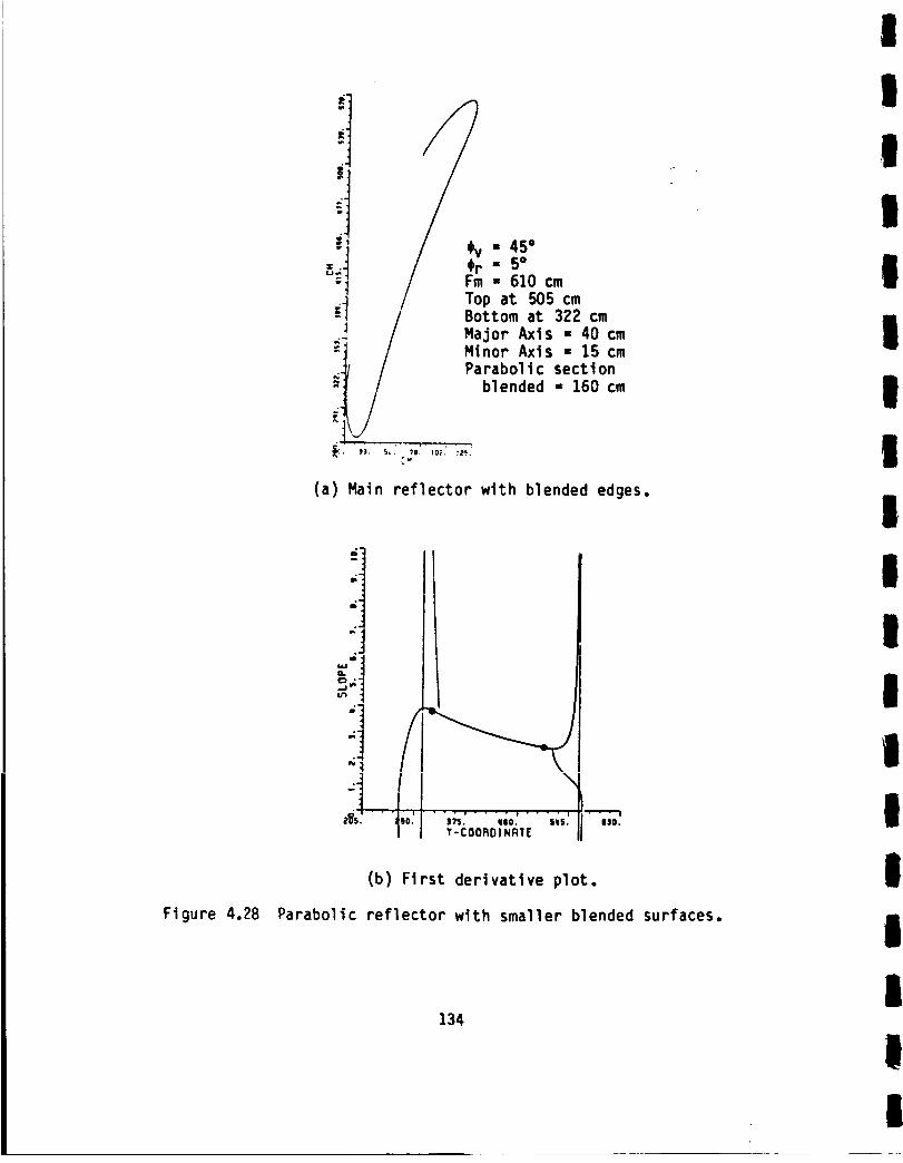
Figure 4.28

o

mr

"I /

:_oFm - 610 cm


Major Axis - 40 cmMinor Axis - 15 cm

Parabolic section

blended - 160 cm

C. 33. $_.''"7g.' IOn.' I_.'

C"

(a) Main reflector with blended edges.

P

,;"

,:-

k2.

/

J11• ",o_" ,,s. ,,o. " ..TI T-COOFID|NRT[


Parabolic reflector with smaller blended surfaces.

134

I

II

I

IIII

II

IIIIi

II

I

i

I!

II

II

III

II

Ii

II

I

Figure

:J

-,.j

7

mu

i

4.28

'".: ;/ I ....... "4 . " ........... " .....

4 . • , . .- .-: • . : : : -: : : : : :

_03. 2S6. )OI. 3S2, q|S. I$1. S_|. $?1. S_?. MO.

DISTRNCE FROM AXIS ICM)

(c) Geometrical optics plot. Frequency = 4 GHz

"L_M ¸::!o-

i : I I 1 .-: :t :-_1_-_.:1_ :

--g--_?::

,ii " 1i i

:.: i, : i :il-- .::I: ::

" i ,-!_..--.-"_I_10. _03. _S$. 309. 302. qtS. qss. S2l . S?li. S27. 1100.

DISIRNCE FROM AXIS [CM)

(d) Moment method plot. Frequency = 4 GHz

(Continued).

135

Momentmethod and GOanalysis are used for the entire system and

the GOreflected field for the entire system will be examined first.

In Figure 4.29, the reflected field from the subreflector that does not

interact with the blended surfaces is given by

with

and

-jk ( Pi+Prl+Pr2)UREF= / Pc1 e

¢ Pi(Pcl+Prl ) (4.148)

Pc1 = [(LV-Xs )2 + Ys 2]I/2

Pi = [(Fc-Lv+xs )2+ Ys 211/2

(4.149)

(4.150)

Now Ym and Ys are related by

Ym = 2Fm[-1/c + /1/c2 + 1] (4.151)

where

c = Ys . (4.152)

vt-_-xs

Also, one finds that

Pr2 = Fm + DISPN - xm (4.154)

YOB = Ym , and

[(Fm.Lv+xs.Xm)2 2 1/2Prl : + (Ym-Ys) ] •

(4.155)

(4.156)

136

iI

I

I

II

II

II

II

l

!i

I

I

I

I

, +I L'" _'*" -'-'""

Figure 4.29 Total reflect.ed field.

l L ", "--__-L F. - L _ I D IllPll

Figure 4.30 Blended surface reflected field.

137

yOi

Points on the subreflector are then chosen and rays traced. The

hyperbola section of the subreflector reflects rays that also extend

outside the parabolic section of the main reflector. The reflection

point on these surfaces must be found differently.

The reflected fields for the top and bottom surfaces in Figure 4.30

are given by

or

and

-jk Pi -jk Prl -jk Pr2

uREF= e .{ 4"/ Pc1 e / Pc2 ePc1+PrI VPc2 + Pr2 (4.157 )

UREF = / PclPc2¢ Pi(Pcl+Prl )(Pc2+Pr2 )

Pi = [(Fc-Lv+xs) 2+ ys211/2

-jk (Pi+Prl+Pr2)e

(4.158)

(4.159)

where xs and Ys are chosen on the subreflector. There are two

possibilities for Pc1. If (Xs,Ys) is on the hyperbola section then

2 2Pcl = [(Lv-xs) + Ys ] (4,160)

Otherwise, Pc1 for the surface s is given by Equation (4.28) and those

that follow it. The reflection point on the main reflector must now be

found. For (Xs,Ys) on the hyperbola, one obtains

^ (a/b2)Ys ^

^ ^ ^ -x + [l+(Ys/b)2]i/2 x= (4.161)

nI = nxX + nyy ' ' ]-- (a/b2)Ys --12 zz2 .

138

I

I

il

II

ilII

II

I!

II

I

I

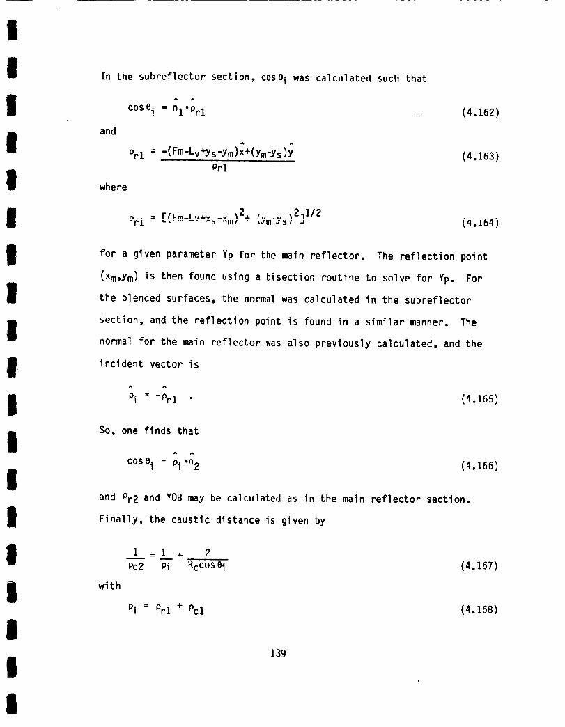
I

I

i

I

I

I

I

IIII

II

I

I

I

In the subreflector section, cos0 i was calculated such that

A

cose i = nl.Prl

and

Prl = -(Fm-Lv+Ys'Ym)X+(Ym'Ys );

Prl

where

9 911'). = rf_m_Iv+v__v _% r,,_,, _i"I_

_ri _, ....... "-_ "-.i, _Jm Js, -

(4.162)

(4.163)

(4.164)

for a given parameter Yp for the main reflector. The reflection point

(Xm,Ym) is then found using a bisection routine to solve for Yp. For

the blended surfaces, the normal was calculated in the subreflector

section, and the reflection point is found in a similar manner. The

normal for the main reflector was also previously calculated, and the

incident vector is

A

Pi = -Prl " (4.165)

So, one finds that

cose i = Pi'n2 (4.166)

and Pr2 and Y0B may be calculated as in the main reflector section.

Finally, the caustic distance is given by

with

I_/_=1+ 2Pc2 Pi Rccos ei

Pi = Prl + Pc1

(4.167)

(4.168)

139

and Rc was calculated previously. Then UREFis knownthrough selecting

points on the subreflector and implementing the above ray tracing

procedure.

In the momentmethod procedure, the entire system is represented by

a geometry of points spaced a variable distance apart. This distance is

usually fixed at two-tenths wavelengths for best results. Nowthe

momentmethodis applied to the entire system (Figure 4.31) and the plot

in Figure 4.32 results. The magnetic line source also reflects off the

main reflector into the target area, and this field is subtracted

yielding Figure 4.33. Next the spillover incident field and the direct

reflected field off the subreflector edge are subracted out yielding

Figure 4.34. The triple reflected field ripple is apparent as well as a

slow varying ripple caused by successive reflections from the

subreflector edge, the main reflector edge, the subreflector hyperbolic

area, and the main reflector parabolic area. Of course in an actual

system, this field componentis not seen by using a pulsed radar system.

Finally, by selectively zeroing the correct elements in the impedance

matrix, the interaction between the main reflector and subreflector is

eliminated resulting in Figure 4.35 where the slow and fast ripple have

been eliminated. The corresponding GOplot is shownin Figure 4.36.

GOmayalso be used to calculate the triple reflected field level

since all the basic analysis has already been completed (see Figure

4.37). First _2 is recalculated and (Xs,Ys) found on the subreflector

using a bisection method. Then Pr2 is known. The normal is computedat

(Xs,Ys) and another bisection method to find YOB. This yields Pr3 and

Pc which may also be calculated at this point.

140

II

l

II

Il

I

II

II

III

Il

I

l

I

l

l

I

I

I

I

I

I

I

I

I

i

I

!

I

.m

C::)

CO

r,_"

¢,DL/')

=;C_IS)

f,.,.

(.....)_

(._"

it')

_J

CC)

o

c,r'_ "

¢.D

\\

\\

\\

\\

,....._.,.,......-,-.-.-

'' '' f' '''{ .... I' '''l ' ' ''1' '' '1 .... I''' 'l'' '' i .... 1

_3. ,,.,_.''_ 169. 232. 295. 35B. _21. _8_. 5_7. o_0."'

CASSEGRAIN SYSTEM [CM]

= 45 °@r = 5

Fm = 610cm

Fc = 610cm

Main Reflector Subreflector

Major Axis = 80cmMinor Axis = 30cm

Parabolic blended section = 320cm

Top edge at 505cm

Bottom edge at 322cm

Major Axis = 20cmMinor Axis = 13cm

Hyperbolic section blended = 80cm

Top edge at 49.4cm

Bottom edge at 30.9cm

Unnecessary edge extensions in back regions have been eliminated.

Figure 4.31 Entire Cassegrain system.

141

i| _i7_i--!77],{1-:-_l:i_ ,ti ili. _iij :i_-_--.l+::_-_t;._-_--iLt_lllli i UI,]_ I1,IltlI1_Jllt..qlll111iltttI.A]A.Es'._Tillnh/lllll&,tlII I'I_II_IlI_LIt_IIlliltlItI]I]IN[I[..tlllllll_JlWI_iil/:17: t lil_l]}l -tll_iiilltlItiltltN

.'_.tlll_lUIll_lJ,ill;I ! l[l]]Jl-l]]ltl _1t111II

:ilw"_lllllri,_ii_',:,:::lI!: 77.1F_llli,ltill ::; @77tI ii::;;ililttit-i_io" itoi. ill. lloli, llll. Ills. ill. ltll. liTi. ill"#. MO.

' fllSTRNCE FROM I:iXI5 ICH)

Figure 4.32 Entire system.

,,, .tiiii 0,..!I_ It' ! '

:;" ! ti_:,,,'.!-:-:_

" i'Jit..... ] lili ,, i ii_-tii. - i)

....tt"t =II1_1)] IIO$. l'ili. IOI. Illll I. IllS. lllllli, lill. i'' _li'll_"" "Ill'?, IlilO.

' DISTRNCE FROM IlXIS ICtll

Figure 4.33 Entire system less main reflector contribution.

142

I

IIII

I

II

II

II

I

III

!

!

!

!

I

I

I

I

I

I

IIi

I

II

Figure 4.34

Figure 4.35

;] -' ..,flnlUl .................... , .... , ..... "IVLAI

........ _ , r I

l l_O. ZO$. _Sli. _lOI. _i62. qlS. q$1l. Y_l. S?ql. IP'?. li$0.. DISTRNCE FROM RXI$ EMI

Entire system less main reflector, subreflector andspillover contribution.

.i____:!_ii !'_'L'__'i

It0. I0). ;PSi. 309. Ilia. II I S • 1168. S21 • 171., OISTRNCE FROM RXIS (CM)

---t

Ili27. IIlO,

Desired reflected field.

143

. ;.; - ;•_.-; ; . _ . fT,_¸. . . . ' . • '_ ._ ....... _ .... 7 . ._-i-i! i__iit_i_!/i: i_IZ_ _1_ _ I__ i \!il _ ._1:_

" _i ill ._i_t_ -i__i i _: _i_1!.\_,_i __ti" .................'....'_:--li_ii} ! ,__._ :iX ......

i'l

in

ill, . • . f. - . , .....

.............___."! _: ....._ _l}=.+l.... .....,\_._:_-.i_._ ._ i

im .

-;;:17-! ........ .................. _ ........

ol i .......ilO. 203. 256, 309. 362; illS. 1687 $21 571_ 627_ 680_

DISTRNCE FROM RXIS (CM)

Figure 4.36 GO reflected field.

144

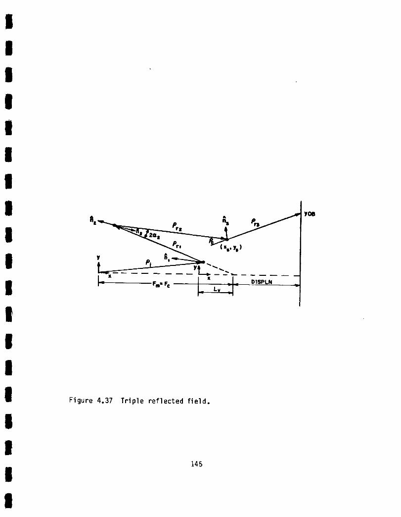
II

I

Ii

I

i

lI,

I

I

II

I

II

l

"- ('o' Y.)

y A,

r rm-Fc

Figure 4.37 Triple reflected field.

145

y_

Then

uYOB -jk Pr3

Pc+Pr3 (4.169)

A plot of this field is shown in Figure 4.38. The level of this field

is plotted relative to the reflected field magnitude in the center of

the target zone. The triple reflected field is actually higher than

that which would be given by the maximum level in Figure 4.38. This

could be remedied by using a more accurate value for the reflection

coefficient when computing the triple reflected field.

At this point, little else can be done about the triple reflected

field without sacrificing the desired flat field performance. One

alternative is to place microwave absorber in the vicinity of the

subreflector to block the ray path of the triple reflected field from

the subreflector to the target area. This improvement could be easily

implemented. In actuality, the triple reflected field will be weaker in

a three-dimensional system in that additional spread factors will reduce

the triple reflected field even further.

Finally, the source horn is placed at the "origin" for convenience

a_ wpll _ nntim_l n_rfnr'm_nr= I:_cD "in rh_nn'inn hnrnc _nA hnrn

orientation and the close proximity of radar components make this an

ideal location. A typical broadband horn gives the desired flat field

over angles much greater than those considered here. If possible, a

field taper is desired over the blended surfaces which will improve

system performance but the major purpose of the horn is flat, broadband

performance over the widest possible angles.

146

I

I

II

III

I

III

II

I

II

g

I

I

!

i i

I _:_ ...................... ]_[]i],[] ....p' ! i I , _. _ .........

' .].-, ]1 .. - _ - ........................

_" I S5. 225. 295. $&5. ll35. $05. 575. 6_S. 7 ! 5. 705.

i DISTRNCE FROM RXI$ (CM)

Figure 4.38 GO triple reflected field.

147

CHAPTER V

CASSEGRAIN SYSTEM DESIGN PROCEDURE

The Cassegrain system is a viable alternative for providing a

uniform plane wave in a compact range measurement system. A procedure

will be described briefly for designing a Cassegrain system given a

target area dimension as a constraint. No further constraints will be

given but in actuality each individual application will have its own

unique restrictions.

The system described in Chapter IV will be used as an example; that

is to say the target area is to have a dimension of six feet. The main

reflector is considered first. It is convenient to make the vertical

dimension the same six feet. Increasing this dimension will flatten the

field when just considering the main reflector, but this will result in

a larger overall size leading to an increased triple reflected field.

Therefore, the main reflector is kept as small as possible to keep the

I,,I I_.P IC I qC=l IIt:=bL, I:U I Iq:IU q.,U 0 |I|I I| IIIIUI|I. llt_ UV_I Ol I IVbQI |_li_:}t.,i! _J ill/ $.._

chosen to be approximately three times the target dimension. Care must

be taken to make sure the target plane is not in the far field of the

main reflector at the minimum frequency of operation. For this

particular case, the focal length was chosen to be twenty feet.

148

lI

I

II

Il

I

IiII

IIllII

I

I

I

I

I

I

I

i

I

I

I

I

I

I

I

I

I

The edges of the main reflector must be considered next. Only the

field of the main reflector (source at virtual focal point) is examined.

The three blended surface variables are the major axis length, minor

axis length and blended parabolic section length. The blended parabolic

section is fixed at four times the major axis length for the most

effective transition from the parabola to the blended surface . The

major axis length should be increased until the field over the target

area is flat. The natural taper of the field will also be present.

Some rounding of the field at the junctions will be tolerable since the

subreflector field is usually tapered and will compensate for this

problem resulting in a smooth field at the junctions. Finally the minor

axis length is usually one-third to two-thirds the major axis length.

The actual length is set such that the minimum radius of curvature of

the edge is greater than a quarter wavelength at the lowest frequency of

operation. The rounding of the field at the junctions for this case had

a 0.1 dB to 0.2 dB variation as is seen in Figure 4.27d of the previous

chapter.

The subreflector is designed next. The goal is to generate a

uniform field illuminating the parabolic section of the main reflector

with a subreflector whose overall dimensions are kept as small as

possible to reduce field interactions between the two reflectors. One

parameter that determines the size is Cr. For this example a value of

five degrees was chosen. The blended surfaces are added next

following the same procedure as with the main reflector. The far field

pattern is then examined and a half dB variation over the area to be

149

illuminated is tolerable. In Figure 4.12b the subreflector field plot

is shownand the desired illumination area is from 135° to 150 ° for this

particular example. If the field variation is not acceptable, the size

of the blended surfaces may be increased. If a flatter field is not

obtained, the size of the hyperbolic reflector section must be

increased, and the addition of the blended edges repeated until a

satisfactory pattern is obtained.

The total system may then be put together, and the resulting

pattern examined. The feed is placed beneath the main reflector at the

"origin". Although the feed could be placed somewhere between the

reflectors, this location is most operationally convenient and gives

good source performance since the beamwidth is smaller and field flatter

at this increased distance. The system is now completely specified, and

little further design may be done except for varying the offset angle

between the two reflectors. Increasing this offset angle without

altering the rest of the system should reduce the triple reflected

field. The interaction between the blended surfaces of the reflectors

now results in weaker reflected fields at each edge yielding an overall

reduced triple reflected field. This also changes the desired field

pattern somewhat since the positioning of the hyperbolic subreflector

and parabolic main reflector has changed. This change usually does not

affect the desired pattern greatly but the triple reflected field is

reduced. Therefore, the ideal situation is to have a maximum offset

angle to reduce the triple reflected field making sure that the desired

field over the target area remains acceptable.

150

II

I

iI

I

Ii

IIII

I

I

III

Il

III

II

II

III

I

II

III

I

For this example, consider three cases with offset angles of 35°,

45°, and 55°. A system with ¢v = 35° is shown in Figure 5.1. The

minimum triple reflected field from Figure 5.2 is about 1.6 dB. The

desired reflected field with interactions between reflectors eliminated

is shown in Figure 5.3. Within the six foot target area there is about

0.5 dB rolloff at the extremes. There is about 0.2 dB variation over

4.8 feet of the area. The next case in Figure 5.4 has Cv = 45° and was

the system considered in the previous chapter. At this angle the triple

reflected field is reduced to about 0.9 dB (see Figure 5.5). The

desired reflected field has a 0.4 dB rolloff within the six foot area

and 0.2 dB variation over 5.4 feet (see Figure 5.6). The final case has

@v = 55° as shown in Figure 5.7. The triple reflected field has now

been reduced to a level of 0.6 dB (see Figure 5.8). This change of 0.3

dB is not as great as the reduction between the angles of 35° and 45°

which implies diminishing returns with increasing angles. The desired

reflected field has less than 0.4 dB rolloff within the six foot target

area. And 0.2 dB variation over 5.4 feet as shown in Figure 5.9.

Therefore, a maximum offset angle is desired but this must be tailored

to each individual case. Note that the polarization performance will

deteriorate with increasing tilt angle for a full three-dimensional

system.

151

-_0 .' 2 5. 90.

\

155. 220. 285. 350. 415. 480. 545.

CASSEGRAIN SYSTEM (CM)610.

= 35 °@r = 50

Fm = 610 cm

Fc = 610 cm


Major Axis = 80 cmMinor axis = 30 cm

Blended parabolic section

Top edge at 384 cm

Bottom edge at 201 cm

= 320 cm

Major Axis = ZO cmMinor Axis = 13 cm

Blended hyperbolic Section = 80 cm

Top edge at 47.4 ccm

Bottom edge at 24.5 cm


Figure 5.1 Cassegrain system with @v = 35°-

152

I

II

II

II

II

III

I

Im

II

I

l

l

I

I

I

I

I

I

I

I

I

I

l

I

l

I

I

-_ , A_I, ,- , __;:_,,• !_-'-_-+:____

if':_-;---;-J-i-- i::I-_+T' -_-m-- _- fill.... _---.! _._"_. _! ] IIIIIIIIIII II •

-.- _:_ _-_.- :_...... ,vl_llillI-_-._ _ _-_-_-__i_::_::::r.__::_ -_ ---_-_""_-_-,- _::_.___.--_ " ' ._ ..;_.L..__'_-_-_ -r_-- -1-4-;--_i._.__ "----i ,--L-;-_-_-

I_I, Ill, _011, }S:', di'l$, alSO, H! • tllq, ql?. llO.

' DISTANCE FROM AXiS ION)

Frequency = 4 GHz

Figure 5.2 Moment method plot showing triple reflected field.

$i

mi

i

• ,.i .... I .... I ...... i ....

la$o 155. :'09, a5Z, 295. 3030. SOt. qaq. q67. $10.

OISTRNCE FROM RXI$ ICM)

Frequency = 4 GHz

Figure 5.3 Moment method plot of desired reflected field.

153

Main Reflector

I

II

• I

I

\\\\ I

_? ?<L--.... \-- I

• 232. 295. 358. q21. qBq. 5q7. 610.

C_SSEG_RIN SYSTEM (CM)



Top edge at 505 cm

Bottom edge at 322 cm

@V = 450(hr = 5°

Fm = 610 cm

Fc = 610 cm

Subreflector

= 320 cm



Top edge at 49.1 ccm



Figure 5.4 Cassegrain system with @v = 45°.

154

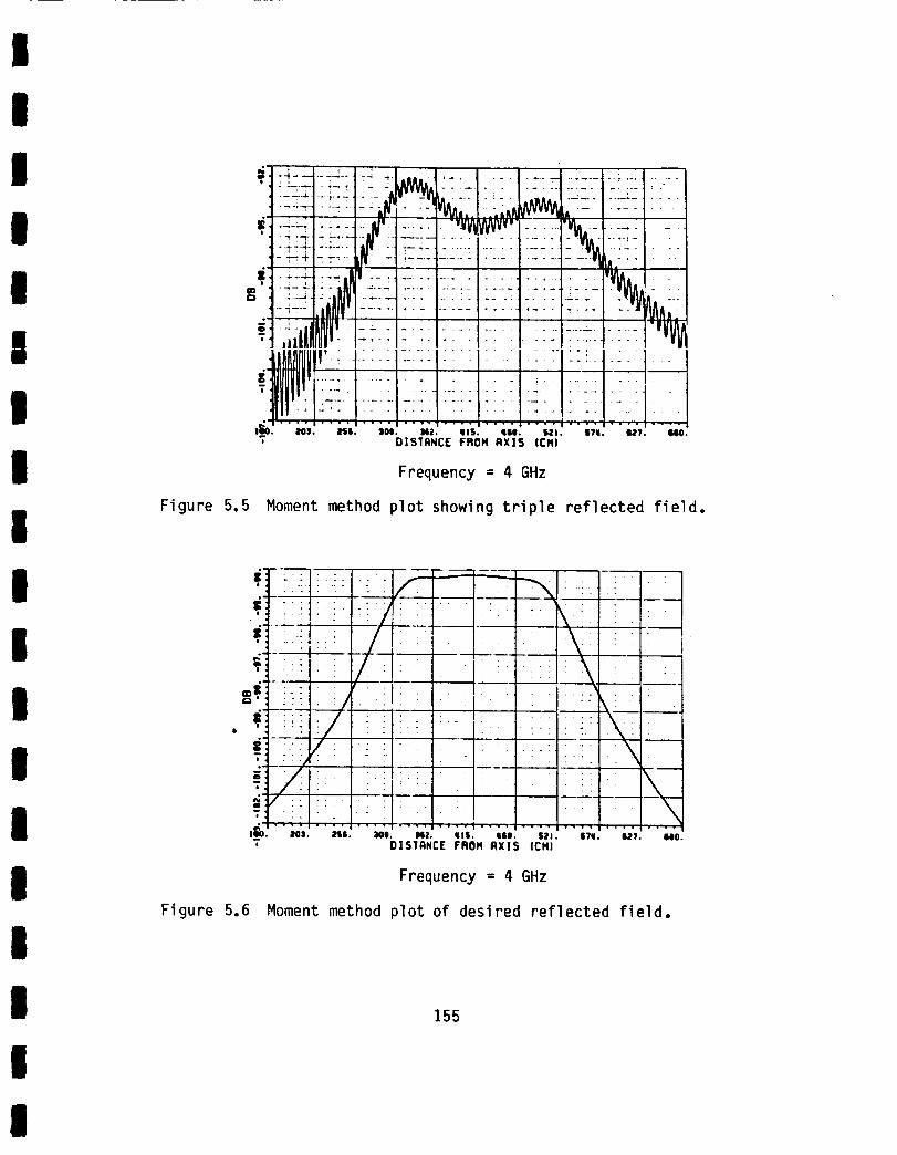
I

I

|

li

I

| ° • • o , • • • • • •

' DISTANCE FROM AXIS ICMI

Frequency = 4 GHz

Figure 5.5 Moment method plot showing triple reflected field.

II

II

I

II

o.

./

T:

20$. ZS6.

q

3NH. N2. IllS. qlli. S;PI. $?q. $_9. lie0.DISTANCE FROM AXIS ICM)

Frequency = 4 GHz

Figure 5.6 Moment method plot of desired reflected field.

155

o.

|

°

{_0 i

\\

\\\

\

\\\\\

\ \\ \\\ \\ \\ \

Bl. 122. 183. _. 305. 365. _27. llO8. .51_%. 610.

CRSSEGR_qIN 5_'STEM (CM)

_V = 550

@r = 50Fm = 610 cmFc = 610 cm




Top edge at 635 cmBottom edge at 452 cm

= 320 cm



Top edge at 50.29 cm



Figure 5.7 Cassegrain system with @v = 55°.

156

II

II

I

II

III

II

II

II

I

I

II

!

s,"i

,,i

! ,

Figure 5.8

i '

| -_

| ®--,"

, i

5

-- $78. q_t, qsq. SOT. SSO. SS$. S$8.' DISTRNCE FROM RXIS (OH)

Figure 5.9

I

_-_"i_;_-i! :- :!'_l: :!', ',:l: .!_ _!-T- -.--;+ .i-' ...... ;-::

• : "'Z _ ...... T" " " .'A _l; " " | ? ..... "_ --TT ' ......

__-_: _'" F': " "iv" _'" ................. ""'"

**_ i_c_!l?;i.... _ ;::.Aj_t;",]i!i:zJ._-'.-:ili]::iL:F:T]r_]_: _lL "_ "

. ._ ,_ . _ ................... _. . _J_ • : • - _

|lllUUi T : Z i i _ , : ,w..

!! :_t-:_i :.:!.'_!_!.2_.!:!! ! ! i :1: _ :_ !_ i i._: :i i1_i!.i.!t T: !i

875. ?:_. 7SS.

Frequency = 4 GHz

Moment method plot showing triple reflected field.

........ i ..........

/[

ii̧j378. q2l. qSq. S07. SSO. sg$. 838. 87g. 72_. 7SS.

DISTANCE FROM RXIS tOM!

Frequency = 4 GHz

Moment method plot of desired reflected field.

157

CHAPTER VI

CONCLUSIONS

In conclusion, the Cassegrain system will provide a uniform plane

wave but the triple reflected field ripple must be reduced through

judicious design and absorber blocking. The blended edges provide

superior performance over large target areas for a given size reflector

system. Design and analysis is best implemented by studying the main

reflector and subreflector separately. Then the system may be put

together to complete the analysis.

Different techniques were used to study the system. The moment

method provides accurate results but is limited by structure size and

computational speed. Though difficult to implement in some situations,

UTD provides results which compare favorably with moment method even

when just examining the reflected field. UTD is also fast and usable on

large structures. Both these techniques are best utilized by examining

path rpfl_rtnr _np_r_t_lv h_fnr_ rnmhJninn _nrl rh_rklnn @h_ @n@_l

system.

With the two reflector system, the elimination of undesired field

components becomes the prime consideration. Those field components

which have pathlengths that differ greatly from the desired reflected

field pathlength may be eliminated through time gating with the use of a

pulsed radar system. The triple reflected field component does have a

158

lI

II

II

II

II

II

II

,lI

I

I

l

III

I

I

IIII

I

Il

II

II

similar pathlength to the desired reflected field and must be reduced

through careful design of the two reflector system. If

three-dimensional effects were also considered, the apparent level of

this field would be reduced further. Absorber blocking around the

subreflector would also reduce the triple reflected field at the expense

of introducing diffracted components from the absorber. The diffracted

fields from all blended surface junctions have been virtually eliminated

through the blending process.

This report is not a complete study of this topic, but it serves to

illustrate the potential benefits and problem areas associated with

subreflector compact range systems. Further work is needed for

three-dimensional structures in order to give additional insight into

the working of the system as well as give improved accuracy in the area

of several field components. The blending procedure implemented is new

and various blending functions as well asdifferent blending processes

provide additional possibilities for system enhancement. The diffracted

field at the blended surface junction, though not considered here, is

another area of potential analysis. Other Cassegrain reflector system

configurations are possible including the isolation of one reflector

from the other in separate areas to reduce the interaction between the

two. Finally, the actual physical construction and implementation of a

Cassegrain reflector system would provide the final verification of the

analysis and design.

159

APPENDIXA

REFLECTION POINT ON MAIN REFLECTOR

This appendix describes how the reflection point on the main

reflector is found• Knowing that the angle of incidence equals the

angle of reflection, a point, (Xo,Yo) is initially chosen on the

parabola (see Figure A.1). Now the normal is given by

A A #W

n: X__ry

(i + _.z) z/_

A new coordinate system is formed at "0" (see Figure A.2).

the radius of curvature and given by

3/2y2

R = 2f(1 + i[irz)

so "0" is located at

(A.1)

Ris

(A.2)

and

XOR = Xo + 2f(1 +_.z) (A.3)

YOR = Yo - (1 + _z)y • (A.4)

Working in this new coordinate system, move A@ and assume R remains the

same for this small change• Now

cos8 i = cose r

160

I

III

II

II

II

lI

Il

lI

I

I

I

Ii

KNOWN / ^ i

I ,_,,__' 7 I

• 1Z_L^_ I I,

Figure A.1 Initial reflection point.

I

m

I

II _"''

IFigure A.2 New coordinate system.

161

or

and

A A _ A

n .l=n .r

T : (x'x + y'y) - xRcosA+ - yRsina¢ ,

(A.5)

and

F = x(x" - RcosA@) + ;(y" - Rsina¢)

" (x _ +)n = - cosA@ + sinA .

Now as a¢ + O, cosA¢ + 1 and sina@ + a@.

T - x(x'-R) + y(y"-RA@),

So

and

F - x(x"-R) + y(y"-Ra¢),

" (x+;,,+)n m _ •

So Equation (A.5) simplifies (ignoring second order terms, (A@) 2) to

a¢ = (x"-R)2[(x"R)2+(y')2]-(x'-R)2[(x"'R)2+ (y,,)2]

2(x'-R)y' [(x"-R)2+(y,,)2]_2y,,R(x, .R) 2+2y 'R(x"-R)2-2 (x"-R)y" •

[(x'-R)2+(y') 2]

(A.6)

Now moving from this nearby point to a point actually on the reflector,

the error is computed as follows:

A _ ^ A

c = nNEW.INEW-nNEW.rNE W . (A.7)

162

l

II

I

II

II

iI

II

II

II

II

I

I

I

I

I

l

I

I

I

I

I

I

I

I

I

I

I

I

The reflection point is found when the error is below some prescribed

value. Otherwise, the procedure is repeated until the minimum error is

obtained.

For convenience, the point actually on the reflector is shown in

Figure A.3 and given by

YP = Y0R + Rsin(A¢+_)

and

Xp = Yp2/(4f)

where

= TAN-I(Yo/2f).. • (A.8)

(X

A

yoLo

xp,yp/ \ Rco,Z_@Rsi._@)o_o%[ _"_" "_"

O I YO_ _ _ NEW ^

/ _x ,y )

//_ OR OR

/(KNOWN

(x', y')/IN OLD)

EDGE /v

XOLt)

( x", y")

PLANE

Figure A.3 Actual point on reflector.

163

Then I

A A

(1 +'YpZ/4fL)'' I ^

TNEW = (x'OLD - XpOLD )x + (Y'OLD - YPOLD )y ' I

and im II ^ II ^

rNEW - (x OLD - XpOLD )x + (y OLD -YPOLD )y" I

The subscript "OLD" refers to the original coordinate system. The error

is then given by Equation (A.7) as I

_; _ ]- _ I(1 + _)I/z I/(X,oL D _ XpOLD)2 + (Y'oLD " YPOLD )z' lrY, Y rv, v _YPoLD)

_" OLD - "POLD - _" OLD " "POLD I _ - i

/(X"oLD - XpOLD )z + (Y"oLD - YPOLD )'z'

-i

(X"oLD" XpOLD" (Y"oLD" YPOLD)_) ] "

(A.9)

l!

!Finally, the points (x',y') and (x",y") need to be transformed to

the new coordinate system as follows (see Figure A.4):

X I = !

NEW (xOR - x'OLD)C°S= " (YoR - y OLD )sin= (A.IO)

I

II

164

I

I

I i 9.E*

I --_( %"'v°")l ! _' ' "• _o_-_o_o,_/_//,,o_-,o_o'

I ,,',,',_ Y:'°EDGE --"

I (a) (x',y') coordinate transformation.

i

iA

YNEW ( X", y" )R ,_ /.: p._,,,_,, w/ _ ;

-_O YOR

I / , (XoR, YoR )

I ,I

(b) (x",y") coordinate transformation.

Figure A.4 Coordinate system transformation.

165

and

Y'NEW = "[(X0R - X'0LD)sin_ + (Y0R - y'0LD)c°s_]

X II

NEW (Y"0LD - Y0R )sin_" (x"0LD - X0R)C°S_

(A.11)

(A.12)

y01 =NEW (Y"0LD'Y0R)c°s_ + (x'°0LD - X0R)sina "

a

Another method of proceeding is to take the cross product

A A A A

1 xn=nxr

(A.13)

and form

A A ^ ^

n • 1 n .r=

A ^ A A

n × r1 x n

or

or

(n•_)(nxr)--(n•r)(;xn)

A

(n • T)(n x F) = (n • r)(T x n) . (A.14)

A

Using the small argument forms of T, F, and n, Equation (A.14) yields

A¢ = y'(x"-R) + y"(x'-R) (A.15)v'Iv"-_) * ""{x'-R) - _v'v"

when ignoring second order terms. Equation (A.15) may be used as an

alternative to Equation (A.6).

166

II

II

I

II

III

II

II

II

I

I

I

I

I

I

I

I

I

I

I

I

I

I

I

I

I

I

I

APPENDIX B

REFLECTION POINT ON ELLIPTICAL EDGE OF SUBREFLECTOR

This appendix describes how the reflection point on the elliptical

rolled edge of the subreflector is found. In Figure B.I point (s,t) is

known and the normal to the surface of the ellipse is given by

A A A A A

n = XoX + yoy = Bcosvcose - Asinvsine x + Bcosvsine + Asinvcose y .

[B2cos2v+A2sin 2v] 1/2 [B2cos2v+A2si n2v]I/2

The dot product is then formed(B.1)

with

A A

T -n F .n

_1 171

A _T = x +

, (B P_

(B.3)

and

A

_ = -X °(B.4)

Now at point (s,t),

t = fs+g or g = t-fs

SO

y = f(x-s) + t

or

f =y-t

x-s

(B.5)

where for the ellipse

y = Asin0cosv + Bcos0sinv + YE (B.6)

167

a.d |

x = AcosvcosB - Bsinvsin0 + XE . (B.7) I

to find v which gives the reflection point, an initial guess is made.

From Equation (B.5) f is calculated and then the dot product in Equation I

(B.2) calculated. The difference is formed I

If" A _ A

ERROR = I • n _ r • n (B.8)-_r -_T II

and is this behaves nicely, v may be found by successively bisecting the I

v interval until the desired error tolerance is obtained. Once v and

the reflection point are known, remaining parameters may easily be I

calculated finalwhich ly yield the desired field.

l

l

ln j_(, ( s,tl

y:dX*edO _t// ' !i(_._ I

Figure B.I Reflection point on elliptical rolled edge.

168

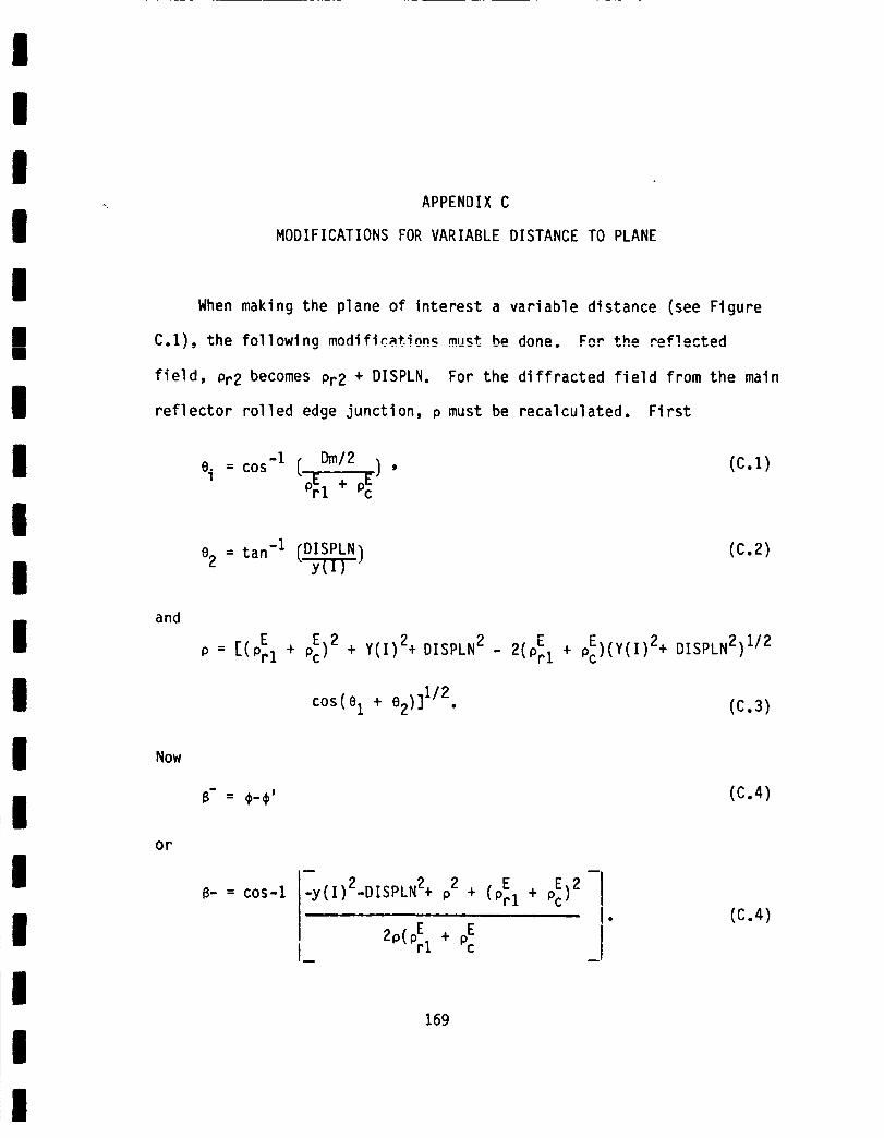
I

II

II

I

II

III

I

III

II

APPENDIX C

MODIFICATIONS FOR VARIABLE DISTANCE TO PLANE

When making the plane of interest a variable distance (see Figure

C•1), the following mndific_tions must be done. For the reflected

field, Pr2 becomes Pr2 + DISPLN. For the diffracted field from the main

reflector rolled edge junction, p must be recalculated• First

Oi = cos-1 ( Dm/2 ) , (C.1)oE. + oE-ri _c

02= tan-1 (DISPLN) (C•2)y---TTT-

and

E E 2 2+ E _ 2+P = [(Prl + Pc) + Y(1) DISPLN 2 - 2(Prl + p )(Y(1) DISPLN2) 1/2

cos(01 + o2)]1/2• (c.3)

(C•4)

or

m

B- = cos-1 .y(1)2_DISPLN2+ p2 +

2p(pErl EI_ + PC

m

E E2 I(Prl + PC)

_1(C.4)

169

I

Next I

B+ = ¢+¢' I

and

0i = 1/2 sin'l( Dm/2 ) I

and pEI+pE I

¢' = 7/2 - 0i.

So I

B+20+(00) Ior

_+:_ _n_C_/12)+_ (C_) 1

PrltPc IFor the diffracted field from the subreflector edge junction,

XOLD = Fm+ DISPLN. I

Finally for the triple reflected field, s goes to Lv + DISPLN. I

DMI 2 _ P IZ__.__2ai _-------_---_ y(I)

__ /I I

_ F - - -Im DISPLN I

Figure C.1 Variable distance to plane.

170

I

III

I

III

II

Ii

I

IIi

[13

[2]

[3]

[4]

[5]

[6]

[7]

REFERENCES

Balanis, C.A., Antenna Theory: Analysis and Design, Harper & Row,Inc., (1982), Chapter 13.

Hanna, P.W., "Microwave Antennas Derived from the Cassegrain

Telescope", IRE Trans. on Antennas and Propagation, Vol. AP-9, pp.140-153, March 1961.

Heedy, D.J., "An E-Plane Analysis of Aperture-Matched Horn Antennas

Using the Moment Method and the Uniform Geometrical Theory of

Diffraction", M.Sc. Thesis, The Ohio State University

ElectroScience Laboratory, Department of Electrical Engineering,Columbus, Ohio, 1984.

Rumsey, V.H., "Reaction Concept in Electromagnetic Theory",Physical Review, Vol. 94, June 15, 1954, pp. 1483-1491.

Schellkunoff, S.A., "On Diffraction and Radiation of

Electromagnetic Waves", Physical Review, Vol. 56, August 15, 1939.

Richmond, J.H., "An Integral-Equation Solution for TE Radiation and

Scattering from Conducting Cylinders", Report 2902-7, October 1972,

The Ohio State University ElectroScience Laboratory, Department of

Electrical Engineering, prepared under Grant NGL 36-008-138 for

National Aeronautics and Space Administration, Langley ResearchCenter.

Burnside, W.D., "Microwave Optics", class notes for Electrical

Engineering course 712, The Ohio State University, 1983.

171

I ,,,, .j ,,3, ' - NASA I I I I I I I I I I I I I I I I I $0272 -T01 REPORT DOCUMENTATIONPAGE I'1"...

Documents

Transcript of I ,,,, .j ,,3, ' - NASA I I I I I I I I I I I I I I I I I $0272 -T01 REPORT DOCUMENTATIONPAGE I'1"...