Sea Ice-Albedo Feedback and Nonlinear Arctic Climate Change

Michael Winton

Geophysical Fluid Dynamics Laboratory/NOAA

Submitted for AGU monograph: Arctic Sea Ice Decline, Bitz and DeWeaver, eds.

15 April 2008

Corresponding author: Dr. Michael Winton, GFDL/NOAA, P.O. Box 308, Princeton University

Forrestal Campus, Princeton, NJ 08542. email: Michael.Winton@noaa.gov

2

Abstract

The potential for sea ice-albedo feedback to give rise to nonlinear climate change in

the Arctic Ocean region – defined as a nonlinear relationship between polar and global

temperature change or, equivalently, a time-varying polar amplification – is explored in

IPCC climate models. Five models supplying SRES A1B ensembles for the 21st century

are examined and very linear relationships are found between polar and global

temperatures (indicating linear polar region climate change), and between polar

temperature and albedo (the potential source of nonlinearity). Two of the climate models

have Arctic Ocean simulations that become annually sea ice-free under the stronger CO2

increase to quadrupling forcing. Both of these runs show increases in polar amplification

at polar temperatures above -5oC and one exhibits heat budget changes that are consistent

with the small ice cap instability of simple energy balance models. Both models show

linear warming up to a polar temperature of -5oC, well above the disappearance of their

September ice covers at about -9oC. Below -5oC, effective annual surface albedo

decreases smoothly as reductions move, progressively, to earlier parts of the sunlit

period. Atmospheric heat transport exerts a strong cooling effect during the transition to

annually ice-free conditions, counteracting the albedo change. Specialized experiments

with atmosphere-only and coupled models show that the main damping mechanism for

sea ice region surface temperature is reduced upward heat flux through the adjacent ice-

free oceans resulting in reduced atmospheric heat transport into the region.

3

I. Introduction

The speculation that Arctic climate has nonlinear behaviors associated with sea ice

albedo feedback has deep roots in climatology (Brooks 1949, Donn and Ewing 1968).

Energy balance models (EBMs) were used to study ice albedo effects starting in the late

1960s and one of the first uses of atmospheric global climate models (GCMs) was to

explore the climatic impact of the Arctic sea ice cover (see review in Royer et al, 1990).

Although climate models show that global temperature change is mainly linear in climate

forcing over a broad range (Manabe and Stouffer 1994; Hansen et al 2005), the nonlinear

relationship between ice albedo and temperature may introduce local nonlinearity.

Simple diffusive energy balance models, that represent this relationship with a step

function, produce an abrupt disappearance of polar ice as the global climate gradually

warms (North 1984). The phenomenon is known as the small ice cap instability (SICI) as

it disallows polar ice caps smaller than a certain critical size related to heat diffusion and

radiative damping parameters. Thorndike (1992) coupled an atmospheric energy balance

model to a simple analytical model of sea ice in an ocean mixed layer, thereby simulating

rather than parameterizing the albedo temperature relationship, and found that seasonally

ice-free states were unstable. Under increased forcing, Thorndike’s “toy” model

transitions directly from annually ice-covered to annually ice-free states inducing a large

and abrupt increase in surface temperature.

The Arctic sea ice cover has been in decline since the 1950s (Vinnikov et al, 1999).

This decline is more pronounced in the summer and recent years have produced striking

record minima (Stroeve et al, 2005). Some researchers have noted that nonlinear

behaviors such as thresholds and tipping points may be associated with this decline

4

(Lindsay and Zhang 2005; Serreze and Francis 2006). The goal of this paper is to assess

the potential for nonlinearity of Arctic climate change in the IPCC fourth assessment

report (AR4) climate models. In section II we demonstrate potential nonlinearities in a

simple model and develop a strategy for assessment. In section III we examine 21st

century simulations for signs of nonlinearity. Section IV continues this search by

examining two strongly forced experiments as they become annually ice-free. Section V

shows that the nonlinear behavior of one of these experiments is similar to the EBM

SICI. Section VI explores the stabilizing effect of ocean surface fluxes and atmospheric

heat transport on the sea ice with special GCM experiments designed to illuminate the

climate response to sea ice region changes. Section VIII summarizes and discusses the

results.

II. Elementary Arctic climate dynamics

The potential for a nonlinear relationship between ice albedo and temperature to

generate nonlinear climate change can be demonstrated with a very simple energy

balance model. Consider the energy balance at the top of an isolated polar atmosphere:

A+BT=S[1- (T)] (1)

The model represents a balance between absorbed shortwave, insolation (S) times a

planetary coalbedo (1- ), and parameterized outgoing longwave radiation with a linear

dependence on surface temperature, T. The model is isolated in the sense that the

atmospheric heat transport convergence is held fixed – bundled with the longwave

intercept into A. The nonlinearity of the model comes from the nonlinear dependence of

on T. At very low mean temperatures, where snow never melts, albedo is insensitive to

temperature. The same is true at high mean temperatures where there is no ice. Between

5

these flat sections, there is a drop from snow to seawater albedos. One might expect,

based on the liquid/ice transition occurring at a fixed temperature, that this drop would

resemble a cliff. However, the seasonal cycle and other variability allow sampling of

various ice-cover states at any given long-term mean temperature, smoothing the

relationship. For simplicity, let's take this smoothed section to be linear and call it the

ramp. The slope of the ramp depends on the drop in albedo between its endpoints and the

temperature range over which the drop is experienced. The drop in planetary albedo, the

albedo above the atmosphere, will be less than the jump in surface albedo because only

part of the insolation reaches and interacts with the surface. There may also be changes

in atmospheric properties with temperature that impact the planetary albedo drop.

Gorodetskaya et al (2006) have used satellite sea ice cover and shortwave data to estimate

the albedo drop for northern hemisphere sea ice regions. They obtain a 0.22 planetary

albedo change for a 100% change in sea ice cover. This is roughly half the surface

albedo difference between a typical sea ice cover and seawater.

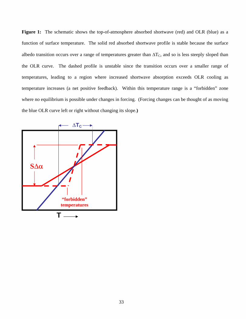
The balance expressed in (1) is depicted schematically in Fig. 1. The steepness of the

albedo ramp, the drop divided by the ramp temperature range, impacts the character of

the nonlinearity. In particular, if the ramp is so steep that, as warming occurs, the extra

shortwave absorption exceeds the extra loss of energy from OLR, the total feedback will

be positive and there will be unstable transitions between ice-covered and ice-free states.

This is an example of the slope-stability theorem of energy balance models (see Crowley

and North, p. 18—19, for an elementary discussion). We can form an expression for the

critical ramp temperature range, TC, between stable and unstable solutions:

TC=S /B (2)

6

A larger range is needed for stabilization when the insolation and the albedo drop are

large and when the longwave damping is small.

Figure 1 shows schematic examples of sub- and supercritical shortwave absorption

profiles. When the albedo ramp steepness is supercritical, the total feedback is positive in

the ramp temperature range so it will contain only unstable equilibria. As a result, the

ramp range becomes a forbidden zone, inaccessible with any forcing. As forcing is

slowly varied, these temperatures are skipped leading to a discontinuity in polar

temperature. Since the polar temperature contributes to the global mean temperature, it

would also have a (much smaller) temperature discontinuity when the ramp steepness is

supercritical.

If we insert the insolation at the North Pole (173 W/m2), the Gorodetskaya et al

planetary albedo drop, and a satellite-estimated outgoing longwave (OLR) damping value

(1.5 W/m2/K, Marani 1999) into (2), we get a critical transition temperature range of

about 25oC. This value indicates instability of the transition to a sea ice free climate

because the annual mean temperature over the perennial sea ice today is about -18oC and

the perennial ice-free zone just beyond the maximum ice edge is at about 0oC. Since ice

in this temperature range is producing the satellite-observed planetary albedo drop, the

average slope of the albedo/temperature curve on the way to ice-free conditions exceeds

the critical slope and so the critical slope would have to be exceeded at some point,

producing instability. However, this conclusion depends upon the assumption that

heating from atmospheric transport remains fixed.

But it is unlikely that atmospheric heat transport would not respond to changes in

shortwave absorption. The region north of 70N receives more energy from the

7

atmospheric transport than it absorbs from the sun and together they make up nearly all

of the OLR – the surface flux is small (Serreze and Barry, 2005). Since atmospheric heat

transport is a big player in Arctic climate, it would not likely stand on the sidelines letting

OLR completely balance a large change in absorbed shortwave. Indeed, it is probable

that the Arctic heat convergence is as high as it is because it is countering the smallness

of Arctic shortwave absorption, which is about 1/3 of the global mean (Serreze and

Barry, 2005).

Horizontal temperature diffusion is a simple method of representing heat transport in

an EBM. However, adding diffusive heat transport to the EBM does not eliminate

unstable transitions in all cases. Instead, these diffusive transport models can exhibit an

unstable loss of a finite patch of polar ice as forcing is increased. The instability is called

the small ice cap instability (SICI) and in some ways is a companion to the large ice cap

instability whereby the globe becomes ice-covered after the ice reaches a critical

maximum extent. The ice edge lies in a temperature boundary zone having a length scale

determined by the diffusivity and longwave damping parameters (North 1984). Both

instabilities occur when this zone impinges on a boundary, either the equator or the pole.

The instability can be removed by reducing the albedo ramp slope but the main point here

is that the instability can occur in spite of down-gradient (warm to cold) transport. At

least in some configurations, the instability is also robust to the inclusion of a seasonal

insolation cycle (Lin and North 1990).

Furthermore, we expect that the transport changes in response to CO2 increase will

have a significant up-gradient component. In the atmosphere this comes about because

warmer air allows for an increase in the latent heat transport. Held and Soden (2006)

8

show that increased latent transport drives an increase in heat transport to the polar

regions, in spite of enhanced warming there, in both equilibrium and transient CO2

increase experiments. Additionally, Holland and Bitz (2003) have shown that the ocean

also transports more heat into the Arctic, even as the heat transport is being reduced at

lower latitudes in association with the weakened meridional overturning circulation.

Thus, it is not clear that heat transport can be relied upon to stabilize Arctic climate by

exerting a cooling influence on the region as it warms at a larger-than-global rate.

When evaluating the linearity of polar climate it will be useful to note the well-

established fact that the global temperature response to forcing is linear. This was clearly

shown for the GISS model by Hansen et al (2005) who calculated forcing efficacy, the

ratio of global temperature change to forcing magnitudes for various forcing types and

magnitudes. The efficacy was constant over a large range of magnitudes including the

last glacial maximum and the anthropogenic future.

We can make use of the global linearity as follows: since global temperature change

is linear in forcing, if polar temperature change is linearly related to it, then polar

temperature change must also be linear. The ratio of polar to global temperature change

is called the polar amplification. It is typically larger than one for a number of reasons

including the ice-albedo feedback. If the polar amplification is also constant then polar

climate change is linear. If there is a nonlinear relationship between polar and global

temperature, a non-constant polar amplification, then the polar change must be nonlinear.

Unstable behavior is a subcategory of nonlinear behavior. If the relationship between

polar and global temperature is nonlinear and shows a temperature discontinuity, we have

evidence of an unstable polar climate change.

9

III. Arctic linearity in 21st century experiments

Now we turn to the GCMs to see whether the projected 21st century polar climate

change exhibits nonlinearity. Since Arctic climate is quite variable, it will be useful to do

some averaging to bring out the forced signal. First, to form TP, the change in polar

surface air temperature, we average over the “half-cap” polar region north of 80N

between 90E and 270E in the coldest part of the Arctic Ocean. In the remainder of this

paper this region is referred to as the polar region. Next we take 5-year averages and we

also average over the separate runs of the individual models made available in the AR4

experiment archive, thus each point represents an average over 15 to 35 years, depending

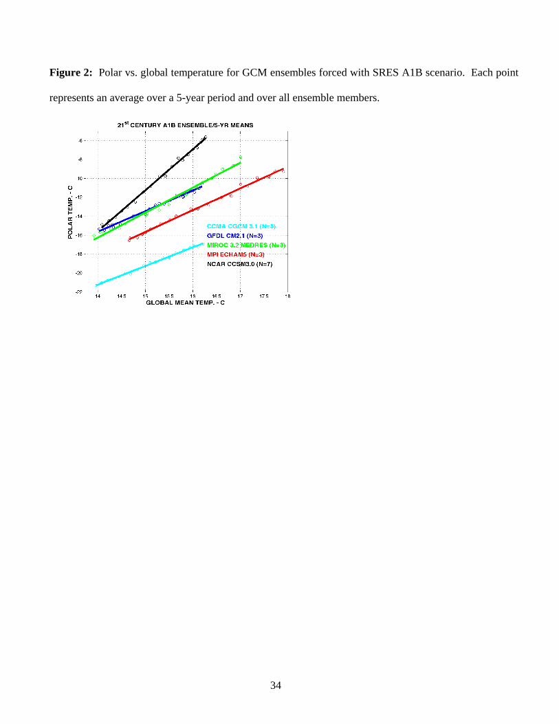
upon the model’s ensemble size. Fig. 2 shows the results for five models that supplied

multiple runs to the archive for the SRES A1B experiment. In spite of differences in

global warming, polar warming and polar amplification, all of the models show a very

linear relationship between polar and global temperature change. From this close

relationship, it is clear that simulated 21st century polar climate change is very linear.

While linear, the polar temperature changes are quite large in some of the models,

comparable to the magnitude of the larger warmings at Greenland during the Dansgaard-

Oeschger cycles (Alley 2000).

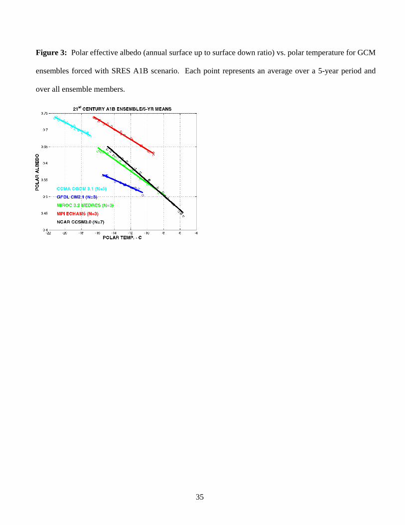
Figure 3 shows the relationship between polar region effective albedo and surface

temperature. The effective albedo is the long-term ratio of surface up to surface down

shortwave flux. Effective albedo can be shown to be the time averaged albedo weighted

with the surface downward shortwave. This weighting is especially important in the

Arctic where the insolation has a very large seasonal cycle. In general, the albedo and

temperature have close linear relationships. Four of the five models become ice-free

10

during September in the polar region over the course of the 21st century without

disturbing this relationship. In terms of the EBM discussion of the last section, the

simulated Arctic climate changes are linear because the albedo/temperature relationship

stays entirely within a subcritical linear ramp region during the 21st century.

The NCAR (National Center for Atmospheric Research) CCSM3 model, which spans

the largest range of temperatures and albedos, shows some gentle downward arcing in its

albedo/temperature relationship (Fig. 3). Since this arcing is not apparent in the polar

amplification plot, other feedbacks must be compensating for its slightly nonlinear

impact. An examination of a similar plot for the planetary albedo (not shown) does not

show this arcing behavior, so the compensation may occur between atmospheric and

surface shortwave terms.

Holland et al (2006) have noted that there are abrupt declines in September Arctic sea

ice cover in the individual ensemble members of the NCAR CCSM3 SRES A1B

experiments. Part of the steepness of the ice cover decline must be related to an

acceleration of global warming in the early 21st century under SRES A1B forcing.

Holland et al report that the annual mean ice cover in the NCAR CCSM3 is linearly

related to global mean temperature, a result earlier found in the UKMO (United Kingdom

Meteorological Office) HadCM3 model by Gregory et al (2002), but that September ice

cover is not so related. Therefore another factor must be involved in these sharp declines.

They note that ice cover responds more sensitively to melting when it is thin. Part of the

acceleration of the ice cover decline and its increase in variability are likely due to this

increased sensitivity. It is to be expected that a binary variable such as ice cover will

show some degree of nonlinearity when confined spatial and temporal averaging is done.

11

The abrupt September ice cover declines are perhaps best characterized as a nonlinear

response to linear climate dynamics.

IV. Arctic nonlinearity in annually sea ice-free experiments

From Fig. 3 we note that, even with the complete loss of September ice in most of the

models, effective albedo has a long way yet to fall to approach open water values of

about 0.1. Furthermore, following their linear trends, the models would achieve this

albedo at temperatures well above freezing – between 11oC and 29oC. The curves would

therefore likely experience considerable steepening under further warming – potentially

inducing nonlinear climate changes.

We can only be sure of establishing the presence or absence of nonlinear behaviors

associated with ice-albedo feedback in experiments that warm to the point of complete

ice removal. Beyond this point there can be no further reductions in polar ocean surface

albedo. The presence or absence of sea ice is easily determined by examining air

temperatures in the coldest month and annual effective surface albedos (the ratio of

annual surface-up to annual surface-down shortwave fluxes). If the coldest month

temperature is at freezing and the effective albedo is near an open ocean value (about 0.1)

then we can be assured that there is little sea ice in the particular region in either summer

or winter. Seventy nine runs of four standard experiments (1%/year CO2 increase to

doubling, 1%/year CO2 increase to quadrupling, SRES A1B and SRES A2) were

examined for annually ice-free conditions in their polar regions (80N-90N, 90E-270E)

based on these criteria. Of these, only two, had years with February polar region

temperatures at freezing temperature and annual surface albedos below 0.15. Thus, it is

quite uncommon for a model’s Arctic ocean to become sea ice-free year around in these

12

climate change experiments. By contrast, it is common in these runs for the Arctic sea

ice to disappear in September – about half of the runs had Septembers with surface

albedos less than 0.15. Unlike Thorndike’s “toy” model, the seasonally ice-free state is

apparently quite stable in GCMs.

The two runs which lose their Arctic sea ice year around are the 1%/year CO2

increase to quadrupling experiments of the MPI ECHAM5 and the NCAR CCSM3.0.

Eleven other models supplying data for this experiment did not lose all Arctic sea ice. Of

the four forcing scenarios, the quadrupling experiment attains the highest forcing level,

over 7 W/m2. Both models are run for nearly 300 years, well past the time of

quadrupling at year 140. The atmospheric CO2 is held constant after quadrupling but

temperatures are generally still rising in the models as the ocean heat uptake declines

(Stouffer 2004).

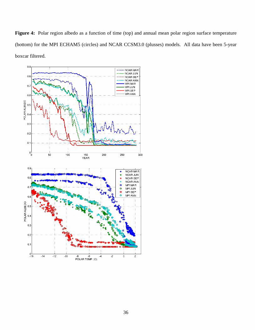
The top panel of Figure 4 shows surface albedo for the polar region as a function of

time for the two model experiments. The seasonal ice state is indicated by the albedos

for three months: March (blue), June (green) and September (red). The annual effective

albedo (light blue) characterizes the time-mean reflective capacity of the ice pack. The

NCAR model loses its September sea ice near year 50, the MPI model loses it later, at

about year 100. Both models have a progression of albedo reductions moving to earlier

months in the sunlit season over the course of the integrations. The March sea ice is lost

abruptly in the MPI model in the CO2 stabilized period. The March decline is more

gradual in the NCAR model. The variability of March albedos after the decline indicates

occasional reappearance of ice in the NCAR model but not in the MPI model.

13

The lower panel of Figure 4 shows the albedos as a function of polar region surface

air temperature. The albedo changes are more similar when viewed as a function of

temperature rather than as a function of time but differences remain. The MPI model

albedo declines are more abrupt in temperature as well as in time. Both models become

seasonally ice-free (the September albedo flattens) at an annual polar temperature of

about -9oC. It is noteworthy that this loss of ice does not alter the nature of the decline in

effective annual albedo in either model. This behavior was also noted in the 21st century

plot (Fig. 3). Here we see that the extension to warmer temperatures does involve

nonlinear effective albedo changes – steepened arcing in the CCSM3 and a kink-like turn

in ECHAM5. The total fall in effective surface albedo is over 0.5 in both models but the

effective planetary albedo drop over the experiments is about 0.1 for both models (not

shown), indicating a large role for atmospheric shortwave masking and shortwave

property changes.

The rapidity of the transition to annually ice-free conditions in the ECHAM5 model

and the failure of subsequent variability to produce significant ice are suggestive of an

unstable transition to a new equilibrium. Since the lifetime of sea ice in the Arctic (about

10 years) is short compared to the timescale of CO2 increase (70 years for CO2 doubling),

we can view the ice as passing through a series of quasi-equilibrated states as the

warming progresses. Under this interpretation the rapid transition to the annually ice-free

state in the MPI model bears some resemblance to the SICI of simple energy balance

models which occurs abruptly as a global forcing is gradually raised above a threshold

value.

14

To explore further the connection between the transition and SICI, we look at the

changes in surface albedo feedback (SAF) as the transition progresses. Using the fact

that the model transitions are more similar in temperature than in time (Fig. 4), we

evaluate the surface albedo feedback in three (annual mean) temperature eras: -15oC to -

10oC (perennial to seasonal ice transition), -10oC to -5oC (seasonal ice), and -5oC to 0oC

(transition to ice-free). The ALL/CLR method of Winton (2005) is used to estimate the

SAF. This method uses standard model output to fit a simple optical model and estimate

the impact of surface albedo changes on shortwave absorption.

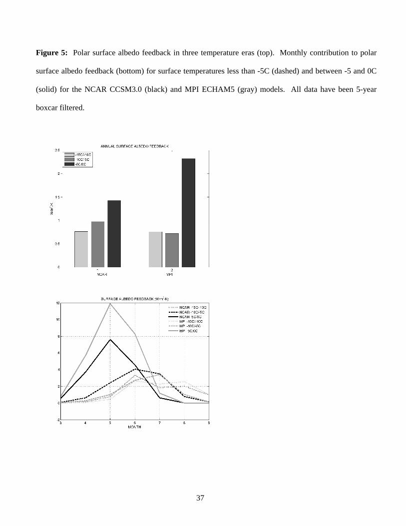
In both models, surface albedo feedback makes an increasing contribution to the

decline in sea ice as air temperatures approach freezing (Fig. 5, top). In the NCAR model

the increase is gradual, consistent with the arcing decrease in effective annual surface

albedo (Fig. 4). In the MPI model a sharp increase occurs in the transition to ice-free

temperature range, consistent with the kinked shape of the effective annual albedo

decline for that model. In the MPI model, the SAF becomes very large (2.3 W/m2/oC) in

the warmest temperature range.

The bottom panel of Figure 5 shows the monthly contributions to the SAF of the two

models in the three temperature ranges. As the warming progresses, there is a shift to

earlier months in the sunlit season. This shift allows the SAF to increase even as the ice-

free season appears and grows. Aside from seasonal insolation variation, the early

months of the sunlit season potentially contribute more to SAF than the later months for

two reasons:

15

(1) Surface albedos are initially larger so there is the potential for a larger albedo

reduction as the ice is removed exposing the low albedo seawater. Figure 4 shows that

September albedos are 0.1 to 0.2 lower than those in March at the beginnings of the runs.

(2) Atmospheric transmissivities are largest in the spring and decline through the

summer to a minimum in September in both models.

Ignoring multiple cloud-ground reflection, the SAF is the product of the downward

atmospheric transmissivity and the surface albedo change, so these two factors compound

each other.

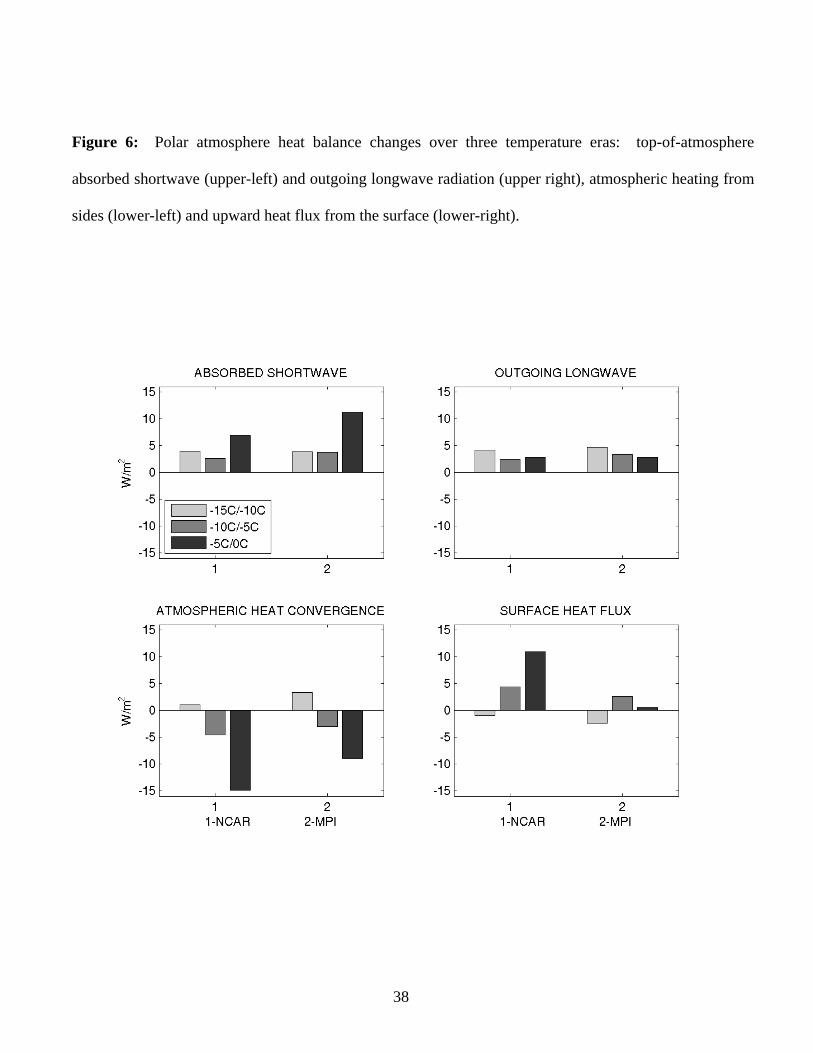
The pattern of surface albedo decline in the CCSM3.0 model (not shown) shows a

plume of reduced albedo penetrating into the half-cap region from the Kara Sea,

indicating an oceanic influence in the decline. This interpretation is borne out by an

examination of the polar region heat budgets for the two models shown in Fig. 6. These

budgets are constructed by regressing the fluxes on temperature in the three temperature

ranges. The slopes are then multiplied by 5oC to give a representative flux change

between the beginning and end of the specified temperature era. Figure 6 shows that the

large increase of SAF in the MPI model at warmer temperatures also appears in the

overall shortwave budget of the region and that there is a smaller increase in the

shortwave budget of the NCAR model. The outgoing longwave radiation has a small

damping effect on the warming of the region in both models. The surface budget changes

are quite different: the MPI model has only small changes while the NCAR model has a

large increase in surface forcing as the ocean supplies increased heating. This ocean

heating contributes more to the warming of the NCAR model in the warmest temperature

era than the SAF. The atmospheric heat transport convergence shifts from a forcing for

16

the warming in the coldest temperature era to damping the warming in the two warmer

eras in both models. It is this change in atmospheric convergence of heat, rather than the

OLR, that does the most to balance the forcing factors: shortwave in MPI, shortwave

plus surface in NCAR. All of the surface flux changes are opposite to the atmosphere

flux convergences in their impacts on the warming.

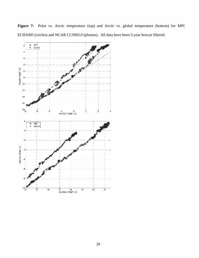
To gain a sense of the regional extent of nonlinear climate changes, we split the polar

amplification into two factors: polar to Arctic (60N-90N) and Arctic to global

amplifications. Figure 7 shows the relationship between polar and Arctic temperatures

(top) and Arctic and global temperatures (bottom) for the two models over the course of

the 1%/year to 4X CO2 runs. The warmest polar temperature attained in the two models

is about the same but the global temperature rise is considerably larger in the MPI model,

while the Arctic/global and polar/Arctic amplifications are correspondingly smaller. The

lines in Fig. 7 are fits to the relationships for data with polar temperatures less than -5oC.

A deviation from this fit at warmer temperatures might reflect the enhanced warming due

to the dramatic changes in sea ice cover above this temperature in both models. The

relationship is mainly linear in both models but in the ECHAM5 model the polar

temperature rises above the reference line starting at a polar temperature of -4oC until it is

about 2oC larger and then begins to parallel the fitted line at a polar temperature of 0oC.

Apparently the large increase in surface albedo feedback in this range of temperatures

(discussed above) plays a role in this extra warming of the polar region. After the ice is

eliminated, the SAF drops to zero, and further warming falls below the -4oC to 0oC ratio.

The behavior of the CCSM3.0 is somewhat different. At -5oC the polar temperature rises

slightly above the fitted line but then parallels it as both regions warm further. In both

17

cases, the transition to seasonally ice free at a polar temperature of -9oC does not disturb

the linear relationship between warming in the two regions. The relationship between

Arctic and global temperatures (Fig. 7, bottom) is quite linear in both models indicating

that the nonlinear changes in the Arctic ocean do not have significant impacts on the

broader region temperatures. Although the elimination of Arctic sea ice would doubtless

have enormous consequences for the local environment, these models do not show it to

be particularly important for the larger scale climate changes.

V. EBM interpretation of the transition to annually ice-free

Now, to provide a mechanistic comparison to the GCM behaviors of the last section,

we examine polar amplification in a simple one dimensional EBM as it experiences small

ice cap instability. Following North (1984), the temperature equation for the EBM is:

)](1)[()1( 2 TxSBTAdx

dTx

dx

dD (3)

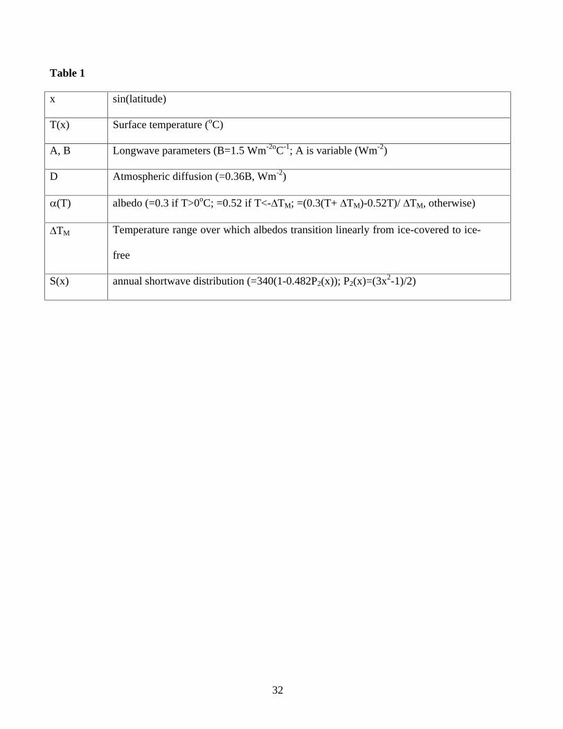
Table 1 defines the notation and gives parameter values. The value for the longwave

sensitivity parameter, B, comes from a regression of ISCCP outgoing longwave on

surface temperature (Marani 1999). The value used for the albedo jump with temperature

is the Gorodetskaya et al (2006) value for the radiative effectiveness of northern

hemisphere sea ice – the impact on planetary albedo of the change from total to zero sea

ice cover. This was determined using ERBE shortwave measurements and HadISST1 sea

ice concentration data. After setting these two parameters, the atmospheric diffusivity, D,

is adjusted to give a reasonable planetary range of surface temperatures.

Most EBM studies explore climate sensitivity by varying the solar constant. Here, we

are interested in exploring the relationship between temperature change at the pole

18

( )1(xT ) and the global mean temperature change (

1

0)( dxxT ) as climate warms. To

this end, it is desirable to force in a manner that does not affect this relationship. So here

we force climate in a meridionally uniform way by varying A – reducing A induces

warming. Thus, we can think of A as a forcing for global mean temperature since

BASdxdxxT1

0

1

0)1()( .

With this forcing, all polar amplification is due to ice-albedo feedback, the only spatially

variable feedback in the system.

Initially we configure the EBM with a step jump in albedo at 0oC ( TM=0oC). North

used -10oC as the location of the step change. This lower value presumably represents

the temperature needed to retain terrestrial snow through the summertime. Sea ice has a

source (seawater freezing) that decreases with increased temperature but is positive while

there are periods of below freezing temperatures. This added source is a factor aiding the

persistence of summer sea ice cover at higher annual temperatures than terrestrial snow.

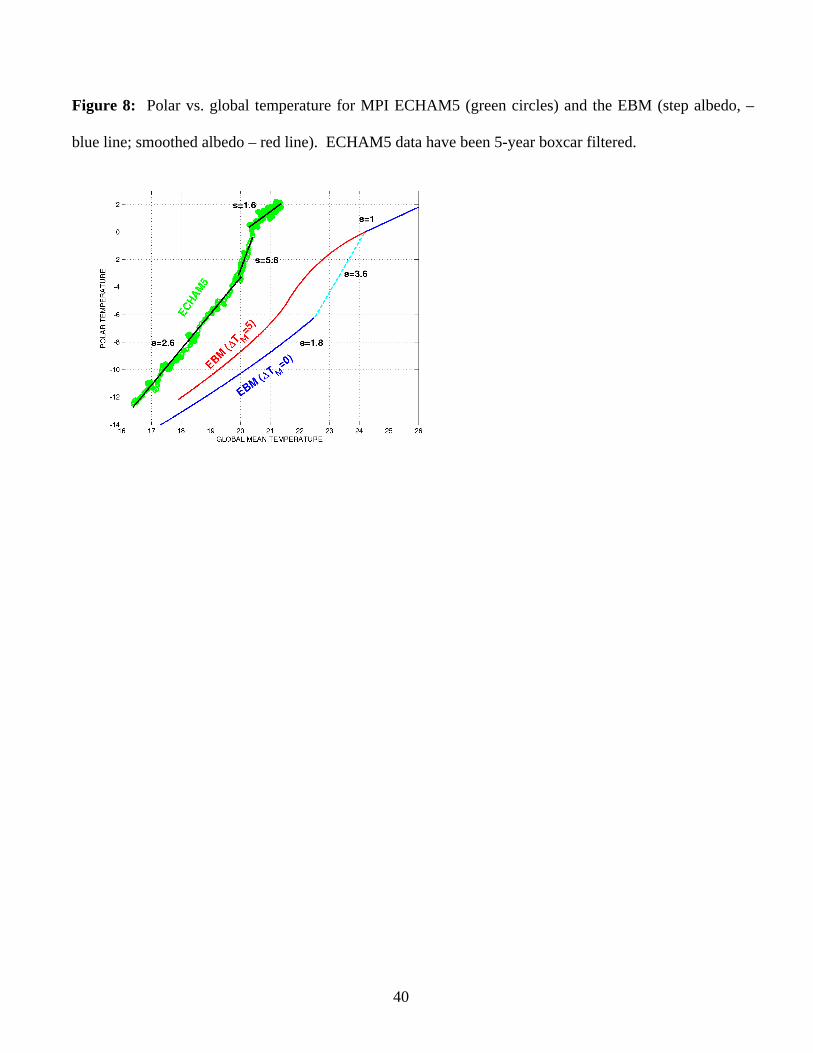
Figure 8 shows the polar and global temperatures for the MPI (Max Planck Institute)

ECHAM5 experiment discussed in the previous section (green) and the EBM with a step

albedo jump (blue) and with the same jump smoothed over a transition zone of 5oC (red).

The EBM changes have been forced by varying A in (3) while the GCM changes are

forced by CO2 increase, of course. The CO2 forcing itself is generally somewhat reduced

in the Arctic (Winton 2006a). Nonetheless, the GCM line is the steepest at each polar

temperature, so the polar amplification is always larger for the GCM than for the EBM.

This is consistent with the finding of a number of studies that factors beside the surface

albedo feedback contribute significantly to polar amplification of climate change

19

(Alexeev 2003; Holland and Bitz 2003; Hall 2004; Winton 2006a). Further evidence of

this can be seen in the MPI ECHAM5 curve where significant polar amplification

remains even after the sea ice has been eliminated. The EBM does not represent these

additional factors and so has smaller polar amplifications.

The EBM with a step albedo change has a discontinuity in polar and global

temperatures where the small ice cap instability is encountered and both warm abruptly

with the removal of the reflective ice cap. The light blue dashed line spans this jump and

its slope defines a polar amplification across the instability. In the cooler part of the

curve, to the left of this jump, the pole is always below freezing temperature so the local

shortwave absorption does not change. The amplification of polar temperature change

over global in this part of the curve, about 1.8, is due to the influence of increased

absorption of shortwave energy at the ice edge, as the ice retreats poleward, conveyed to

the pole by atmospheric transport. North (1984) shows that, as the instability is

approached, the pole feels nearly as much warming impact from the ice retreat as the ice

edge itself.

Based on the fact that the ice cap covers about 6% of the hemisphere before its

elimination, we might expect the polar amplification across the jump to be about 16,

since this increased absorption is the cause of both temperature jumps. The actual polar

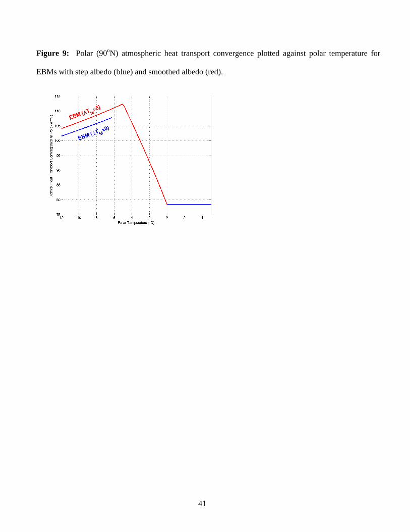
amplification is much less because atmospheric heating at the pole, which has been

increasing to that point, collapses with the ice cap, countering its local impact to a large

degree (Fig. 9). After the ice cap collapse, there is no ice-albedo feedback and polar and

global temperatures rise in a one-to-one relationship. The sequence of changes is in polar

20

energy budget encountered as the climate warms lead to a medium/high/none sequence of

polar amplifications in the EBM.

The global and polar temperatures for the MPI ECHAM5 show a three slope regime

behavior similar to that of the EBM. However, the GCM does not show any

discontinuity in these temperatures. This may be partly due to the GCM, unlike the

EBM, not being fully equilibrated at each point in time and hence able to fill the

“forbidden zone” with transient temperatures. However, taking note that the ECHAM5

sensitivity of polar albedo to temperature is steep but far from step-like (Fig. 4b), we

explore the possibility that having the albedo changes occur over a finite range of

temperatures stabilizes the transition while retaining enhanced polar sensitivity due to

increased surface albedo feedback. EBM runs show that the multiple equilibria remains,

with a reduced T across the jump, for a ramp range of TM = 4 oC but is eliminated

when for TM = 5 oC. The plot for the polar amplification in the stabilized case (Fig 8,

red) shows that a continuous section of enhanced polar amplification fills the region

occupied by the jump in the step albedo EBM. The enhanced sensitivity in this region is

caused by the reduced overall (negative) feedback due to a positive, but subcritical, local

ice-albedo feedback. Figure 9 shows that the diffusive term, operating as a negative

feedback, provides less heating to the pole, opposing the enhanced shortwave absorption.

The change of atmospheric heat transport convergence with polar temperature in Fig.

6 shows that, in the GCMs as well as the EBM, enhancement of polar warming by

atmospheric transport at low temperatures gives way to a damping impact at higher

temperatures. However, the GCM transition occurs at much lower temperature, perhaps

partly due to its having a polar albedo response at lower temperatures. Other

21

mechanisms, not present in the EBM, can significantly impact poleward transport in the

GCMs, for example the enhancement of latent heat transport with temperature (Alexeev

2003; Held and Soden, 2006). As the ice-free state is approached, the damping effect of

the atmospheric heat transport change is much larger than longwave damping in the EBM

as in the GCMs.

VI. The tethering effect of heat transport

The previous section shows that atmospheric heat transport plays an important but

complicated role in polar climate change – initially forcing the region to warm at a

greater-than-global rate but eventually becoming a cooling influence at higher

temperatures. Held and Soden (2006) show that the latent heat component of the

transport scales up in a warming climate according, roughly, to the Clausius-Clapeyron

relationship. This increase drives an increase of the total transport toward the North Pole

in spite of polar amplification. However, it is possible that, even in the early warming,

part of the transport is helping to maintain the very constant polar amplifications seen in

Fig. 2. To expose this moderating role we perform two diagnostic experiments that force

only the polar regions and examine the damping mechanisms.

The first is a modification of the AMIP experiment – an atmospheric model run with

specified sea surface temperatures and sea ice cover. We perform a twin to this

experiment where the sea ice boundary condition is replaced with seawater freezing

temperature and albedo. The experiment is done with the atmospheric component of the

GFDL CM2.1 climate model. A similar experiment for the DJF season was performed

earlier by Royer et al (1990). The impact on atmospheric temperatures and winds in the

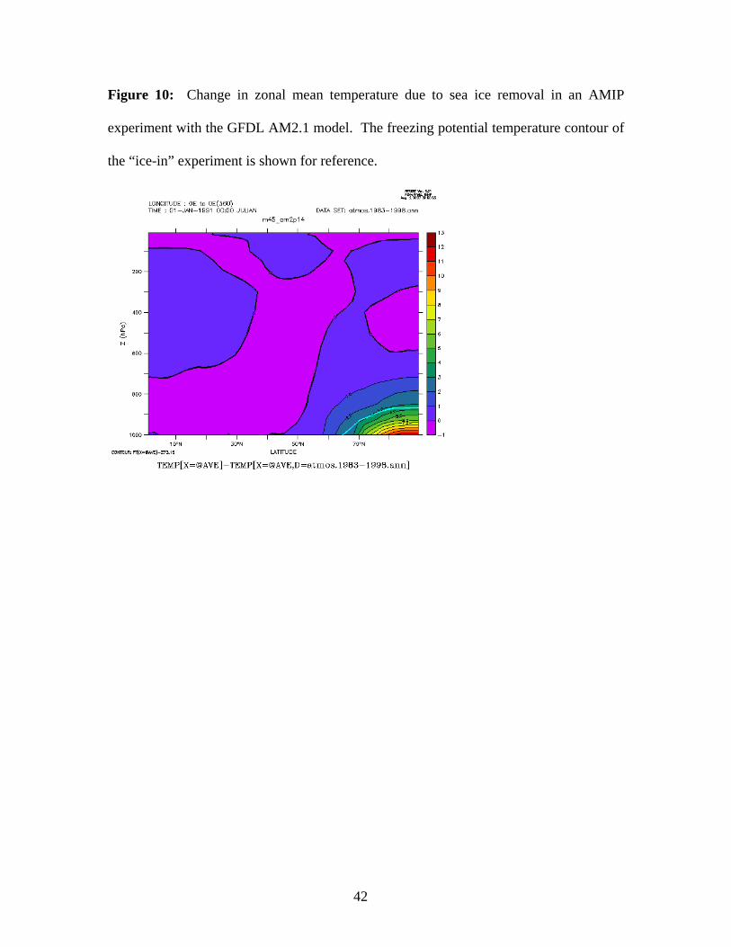
current experiment are in general agreement with those found by Royer et al. Figure 10

22

shows that there is an intense warming of the lower polar atmosphere, mainly confined

below the 0oC potential temperature contour of the control, “ice-in”, simulation. This is

consistent with the regionally limited response of the GCMs to transition to ice-free

conditions shown in Fig. 7. Other features found by Royer et al, an equatorward shift of

the jet, redistribution of sea level high pressure away from the central Arctic to adjacent

land regions, and a reduction of cloud cover as the Arctic Ocean becomes more

convective, are also found in this experiment (not shown).

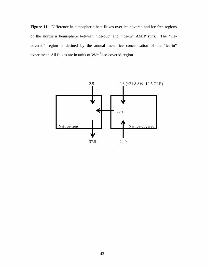
Our main interest in the experiment is to assess the stability of the Arctic ice and its

causes. The net surface heat flux change in the ice-covered regions is the result of two

competing changes: (1) increased shortwave absorption due to lowered albedo, and (2)

increased longwave and turbulent heat loss due to increased surface temperature. The net

upward heat flux change of 24 W/m2 (Fig. 11) indicates that (2) is dominant so the ice is

stable and would grow back at an initial rate of 2.5 m/yr. At the top of the atmosphere,

the extra shortwave absorption is only partly balanced by increased OLR. Most of the

damping influence comes from a reduction of heat transport into the ice covered region

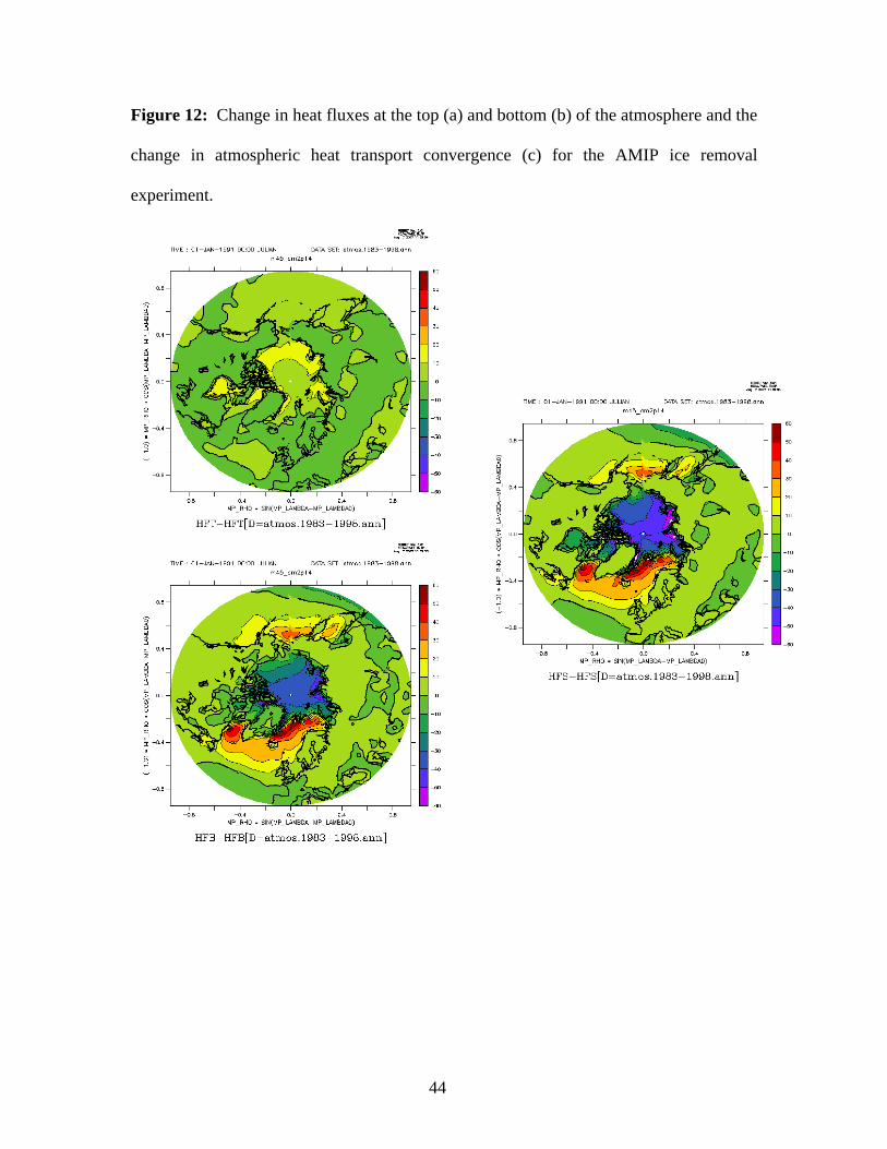
by the atmosphere. This reduced heat transport, in turn, is mainly supported by a

reduction in surface heat flux from the adjacent ice-free ocean, particularly in the North

Atlantic (Fig. 12).

The AMIP experiment fixes SSTs implicitly assuming that the ocean has an infinite

heat capacity. This assumption may be reasonable here since the near-ice regions that are

experiencing large heat flux changes are occupied by deep wintertime mixed layers with

much larger heat capacity than the sea ice or the shallow atmospheric layer that interacts

with it. Nonetheless, it is useful to relax this assumption by performing a similar

23

experiment in a fully coupled climate model – a developmental version of GFDL CM2.1.

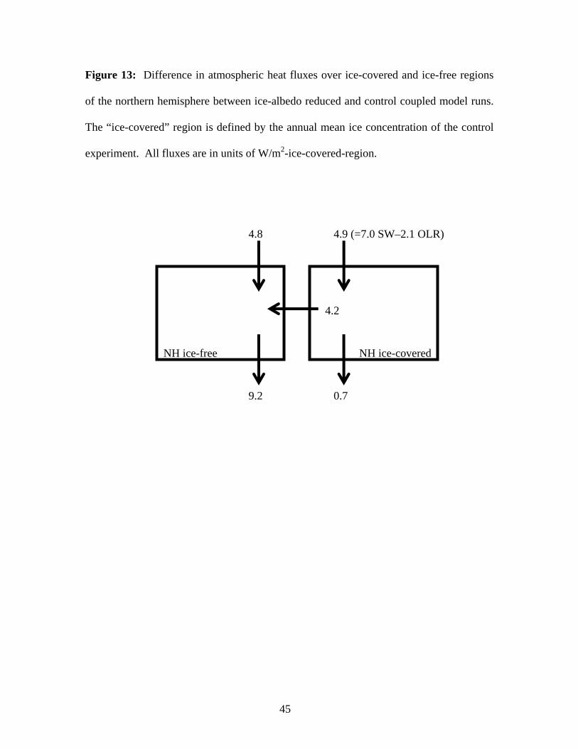
In this 100 year experiment, we force the ice region by lowering the ice albedos. Figure

13 shows changes in climate model heat fluxes as in Fig. 11. As expected, there is an

increase in shortwave absorption at the top of the atmosphere and, as in the AMIP case, it

is only partially offset by a local OLR change. Again the main balancing effect is from a

reduction of atmospheric heat transport convergence into the ice-covered region (defined

from the control experiment). There is also some net downward flux at the surface in the

ice-covered region which is mainly supported by reduced latent heating due to the

reduced sea ice export in thinner ice. This change in sea ice transport has a salinifying

influence near the sea ice edge. Again, the reduced heat transport into the Arctic is

supported by a reduction in heat flux out of the adjacent ocean surface. But this response

is now oversized compared with the changes in the sea ice region. The reason for this is

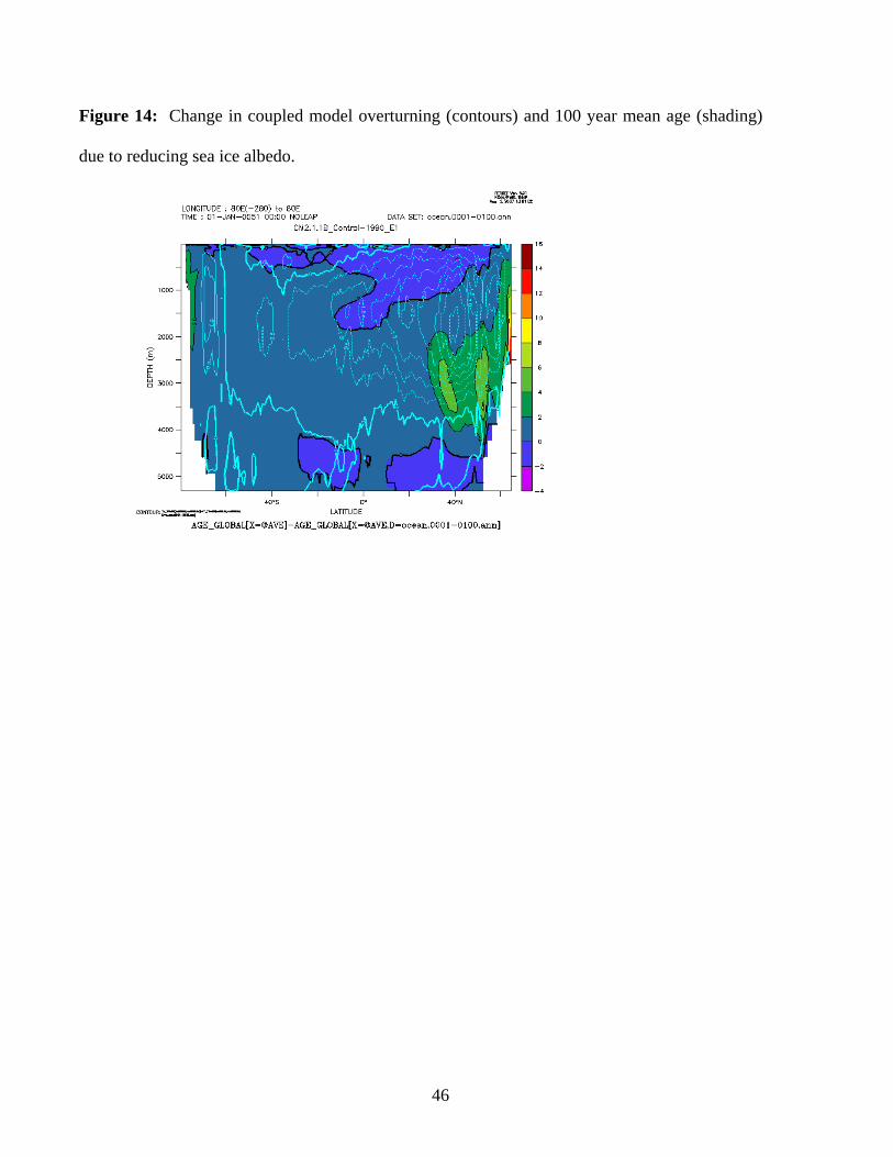
that, in spite of the change in sea ice freshwater forcing, reduced ocean heat extraction

caused by reducing sea ice albedo has induced a reduction of the meridional overturning

circulation (MOC). This is shown in Fig. 14 along with the change in deepwater ages

averaged over the 100 years. The reduction in deepwater ventilation agrees with the

result of a similar sea ice albedo reduction experiment performed by Bitz et al (2006)

with the NCAR CCSM3. The CCSM3 response was relatively larger in the southern

ocean, perhaps because the CCSM3 has more southern ocean sea ice to feel the albedo

reduction than GFDL’s CM2.1.

VII. Summary and discussion

The potential for sea ice-albedo feedback to give rise to nonlinear climate change in

the Arctic ocean – defined as a nonlinear relationship between polar and global

24

temperature change or, equivalently, a time-varying polar amplification has been

explored in the IPCC AR4 climate models. Five models supplying SRES A1B ensembles

for the 21st century were examined and very linear relationships were found between

polar and global temperatures indicating linear Arctic climate change. The relationship

between polar temperature and albedo is also linear in spite of the appearance of ice-free

Septembers in four of the five models.

Two of the IPCC climate models have Arctic Ocean simulations that become

annually sea ice-free under the stronger CO2 increase to quadrupling forcing. Both runs

show increases in polar amplification at polar temperatures above -5oC and one exhibits

heat budget changes that are consistent with the small ice cap instability of simple energy

balance models. Both models show linear warming up to a polar temperature of -5oC,

well above the disappearance of their September ice covers at about -9oC. Below -5oC,

surface albedo decreases smoothly as reductions move, progressively, to earlier parts of

the sunlit period. Atmospheric heat transport exerts a strong cooling influence during

the transition to annually ice-free conditions.

Specialized experiments with atmosphere and coupled models show that

perturbations to the sea ice region climate are opposed by changes in the heat flux

through the adjacent ice-free oceans conveyed by altered atmospheric heat transport into

the sea ice region. This, rather than OLR, is the main damping mechanism of sea ice

region surface temperature. This strong damping along with the weakness of the surface

albedo feedback during the emergence of an ice-free period late in the sunlit season are

the main reasons for the linearity of Arctic climate change and the stability of seasonal

ice covers found in the IPCC models.

25

Support for these mechanisms can be found in simple models. Thorndike's "toy"

model shows their importance by demonstrating the consequences of their absence. In

order to make the “toy” model analytically tractable, the ice experiences a constant

insolation in the summer season. This disables the seasonal adjustment of albedo

feedback just mentioned. Furthermore, the Thorndike model has only weak surface

temperature damping to space through a gray-body atmosphere. Atmospheric heat

transport convergence is held fixed. The result is a model that has no stable seasonal

cycle with ice-covered and ice-free periods -- the model is either annually ice-covered or

annually ice-free. Eisenman (2007) has enhanced the Thorndike model with a sinusoidal

insolation and temperature sensitive atmospheric heat transport and finds stable

seasonally ice-free seasonal cycles over a broad range of CO2 forcings, from 2 to 15

times current levels.

The stabilization of sea ice through opposing heating or cooling of the surrounding

ocean was shown to have substantial impact on the overturning circulation and deep

ventilation. This effect may provide a partial answer to an outstanding question raised by

the CMIP group experiments (Gregory et al, 2002). These experiments separate MOC

weakening under CO2 increase into freshwater and thermally induced components by

using two auxiliary experiments: control radiation with CO2–induced increase in ocean

freshwater forcing and the reverse. These experiments show that the two effects basically

add linearly and that thermal forcing dominates the MOC response. The mechanisms for

this thermal impact are yet to be explored but ice-albedo feedback, and polar

amplification more generally, may be one of them.

26

Acknowledgments: The author thanks Isaac Held, Ron Stouffer, Ian Eisenman, Eric

DeWeaver, Gerald North and an anonymous reviewer for helpful comments on the

manuscript. The author also acknowledges the international modeling groups for

providing their data for analysis, the Program for Climate Model Diagnosis and

Intercomparison (PCMDI) for collecting and archiving the model data, the JSC/CLIVAR

Working Group on Coupled Modeling (WGCM) and their Coupled Model

Intercomparison Project (CMIP) and Climate Simulation Panel for organizing the model

data analysis activity, and the IPCC WG1 TSU for technical support. The IPCC Data

Archive at Lawrence Livermore National Laboratory is supported by the Office of

Science, U.S. Department of Energy.

27

References

Alexeev, V.A., 2003: Sensitivity to CO2 doubling of an atmospheric GCM coupled to an

oceanic mixed layer: a linear analysis, Climate Dynamics, 20, 775—787.

Alley, R.B., 2000: Ice-core evidence of abrupt climate changes, Proceedings Of the

National Academy of Sciences of the United States of America, 97, 1331—1334.

Bitz, C.M., P.R. Gent, R.A. Woodgate, M.M. Holland, and R. Lindsay, 2006: The

influence of sea ice on ocean heat uptake in response to increasing CO2, J. Climate,

19, 2437-2450.

Brooks, C.E.P., 1949: Climate through the ages, 2nd ed., Dover Publications, New York.

Crowley, T.J., and G.R. North, 1991: Paleoclimatology, Oxford University Press, New

York.

Donn, W.L., and M. Ewing, 1968: The theory of an ice-free Arctic Ocean, Meteorol.

Monogr. v. 8, no. 30, 100—105.

Eisenman, I., 2007: Arctic catastrophes in an idealized sea ice model, in 2006 Program

of Studies: Ice (Geophysical Fluid Dynamics Program), p. 131—161, Woods Hole

Oceagr. Inst. Tech. Rept. 2007-2.

Gorodetskaya, I.V., M.A. Cane, L.-B. Tremblay, and A. Kaplan, 2006: The effects of

sea-ice and land-snow concentrations on planetary albedo from the Earth Radiation

Budget Experiment, Atmosphere-Ocean, 44, 195—205.

Gregory, J.M., P.S. Stott, D.J. Cresswell, N.A. Rayner, and C. Gordon, 2002: Recent and

future changes in Arctic sea ice simulated by the HadCM3 AOGCM, Geophys. Res.

Lett., doi:10.1029/2001GLO14575.

28

Hall, A., 2004: The role of surface albedo feedback in climate, J. Climate, 17, 1550--

1568.

Hansen, J., and 45 coauthors, 2005: Efficacy of climate forcings, J. Geophys. Res, 110,

D18104, doi:10.1029/2005JD005776.

Held, I.M., and B.J. Soden, 2006: Robust responses of the hydrological cycle to global

warming, J. Climate, 19, 5868—5699.

Holland, M.M., and C.M. Bitz, 2003: Polar amplification of climate change in coupled

models, Climate Dynamics, 21, 221--232.

Holland, M.M., C.M. Bitz, and B. Tremblay, 2006: Future abrupt reductions in the

summer Arctic sea ice, Geophys. Res. Lett., 33, doi:10.1029/2006GLO28024.

Lin, R.Q., and G.R. North, 1990: A study of abrupt climate change in a simple nonlinear

climate model, Climate Dynamics, 4, 253—261.

Lindsay, R.W., and J. Zhang, 2005: The thinning of the Arctic sea ice, 1988-2003: Have

we passed a tipping point? J. Climate, 18, 4879—4894.

Manabe, S., and R.J. Stouffer, 1994: Multiple-century response of a coupled ocean-

atmosphere model to an increase of carbon dioxide. J. Climate, 7, 5—23.

Marani, M., 1999: Parameterizations of global thermal emissions for simple climate

models, Climate Dynamics, 15, 145—152.

North, G.R., 1984: The small ice cap instability in diffusive climate models, Journal of

Atmospheric Sciences, 41, 3390—3395.

Royer, J.F., S. Planton, and M Deque, 1990: A sensitivity experiment for the removal of

Arctic sea ice with the French spectral general circulation model, Climate Dynamics,

5, 1—17.

29

Serreze, M.C., and R.G. Barry, 2005: The Arctic Climate System, Cambridge University

Press, New York.

Serreze, M.C., and J.A. Francis, 2006: The Arctic amplification debate, Climatic

Change, 76, 241—264.

Stouffer, R.J., 2004: Time scales of climate response, J. Climate, 17(1), 209—217.

Stroeve, J., M.C. Serreze, F. Fetterer, T. Arbetter, W. Meier, J. Maslanik, K. Knowles,

2005: Tracking the Arctic’s shrinking ice cover; another extreme September sea ice

minimum in 2004, Geophys. Res. Lett., 32, L04501, doi:10.1029/2004GLO21810.

Thorndike, A.S., 1992: A toy model linking atmospheric radiation and sea ice growth, J.

Geophys. Res., 97, 9401—9410.

Vinnikov, K.Y., A. Robock, R.J. Stouffer, J.E. Walsh, C.L. Parkinson, D.J. Cavalieri,

J.F.B. Mitchell, D. Garrett, and V.F. Zakharov, 1999: Global warming and Northern

Hemisphere sea ice extent, Science, 286(5446), 1934—1937.

Winton, M., 2006a: Amplified Arctic climate change: What does surface albedo

feedback have to do with it? Geophys. Res. Lett., 33, L03701,

doi:10.1029/2005GL025244.

Winton, M., 2006b: Does the Arctic sea ice have a tipping point? Geophys. Res. Lett.,

33, doi:10.1029/2006GLO28017.

Winton, M., 2005: Simple optical models for diagnosing surface-atmosphere shortwave

interactions, J. Climate, 18, 3796—3805.

Zhang, X., and J.E. Walsh, 2006: Toward a seasonally ice-covered Arctic Ocean, J.

Climate, 19, 1730—1747.

30

Captions

Figure 1: The schematic shows the top-of-atmosphere absorbed shortwave (red) and OLR (blue) as a

function of surface temperature. The solid red absorbed shortwave profile is stable because the surface albedo

transition occurs over a range of temperatures greater than TC, and so is less steeply sloped than the OLR

curve. The dashed profile is unstable since the transition occurs over a smaller range of temperatures, leading

to a region where increased shortwave absorption exceeds OLR cooling as temperature increases (a net

positive feedback). Within this temperature range is a “forbidden” zone where no equilibrium is possible

under changes in forcing. (Forcing changes can be thought of as moving the blue OLR curve left or right

without changing its slope.)

Figure 2: Polar vs. global temperature for GCM ensembles forced with SRES A1B scenario. Each point

represents an average over a 5-year period and over all ensemble members.

Figure 3: Polar effective albedo (annual surface up to surface down ratio) vs. polar temperature for GCM

ensembles forced with SRES A1B scenario. Each point represents an average over a 5-year period and over

all ensemble members.

Figure 4: Polar region albedo as a function of time (top) and annual mean polar region surface temperature

(bottom) for the MPI ECHAM5 (circles) and NCAR CCSM3.0 (plusses) models. All data have been 5-year

boxcar filtered.

Figure 5: Polar surface albedo feedback in three temperature eras (top). Monthly contribution to polar

surface albedo feedback (bottom) for surface temperatures less than -5C (dashed) and between -5 and 0C

(solid) for the NCAR CCSM3.0 (black) and MPI ECHAM5 (gray) models. All data have been 5-year boxcar

filtered.

31

Figure 6: Polar atmosphere heat balance changes over three temperature eras: top-of-atmosphere absorbed

shortwave (upper-left) and outgoing longwave radiation (upper right), atmospheric heating from sides (lower-

left) and upward heat flux from the surface (lower-right).

Figure 7: Polar vs. Arctic temperature (top) and Arctic vs. global temperature (bottom) for MPI ECHAM5

(circles) and NCAR CCSM3.0 (plusses). All data have been 5-year boxcar filtered.

Figure 8: Polar vs. global temperature for MPI ECHAM5 (green circles) and the EBM (step albedo, – blue

line; smoothed albedo – red line). ECHAM5 data have been 5-year boxcar filtered.

Figure 9: Polar (90oN) atmospheric heat transport convergence plotted against polar temperature for EBMs

with step albedo (blue) and smoothed albedo (red).

Figure 10: Change in zonal mean temperature due to sea ice removal in an AMIP experiment with the GFDL

AM2.1 model. The freezing potential temperature contour of the “ice-in” experiment is shown for reference.

Figure 11: Difference in atmospheric heat fluxes over ice-covered and ice-free regions of the northern

hemisphere between “ice-out” and “ice-in” AMIP runs. The “ice-covered” region is defined by the annual

mean ice concentration of the “ice-in” experiment. All fluxes are in units of W/m2-ice-covered-region.

Figure 12: Change in heat fluxes at the top (a) and bottom (b) of the atmosphere and the change in

atmospheric heat transport convergence (c) for the AMIP ice removal experiment.

Figure 13: Difference in atmospheric heat fluxes over ice-covered and ice-free regions of the northern

hemisphere between ice-albedo reduced and control coupled model runs. The “ice-covered” region is defined

by the annual mean ice concentration of the control experiment. All fluxes are in units of W/m2-ice-covered-

region.

Figure 14: Change in coupled model overturning (contours) and 100 year mean age (shading) due to

reducing sea ice albedo.

32

Table 1

x sin(latitude)

T(x) Surface temperature (oC)

A, B Longwave parameters (B=1.5 Wm-2oC-1; A is variable (Wm-2)

D Atmospheric diffusion (=0.36B, Wm-2)

(T) albedo (=0.3 if T>0oC; =0.52 if T<- TM; =(0.3(T+ TM)-0.52T)/ TM, otherwise)

TM Temperature range over which albedos transition linearly from ice-covered to ice-

free

S(x) annual shortwave distribution (=340(1-0.482P2(x)); P2(x)=(3x2-1)/2)

33

Figure 1: The schematic shows the top-of-atmosphere absorbed shortwave (red) and OLR (blue) as a

function of surface temperature. The solid red absorbed shortwave profile is stable because the surface

albedo transition occurs over a range of temperatures greater than TC, and so is less steeply sloped than

the OLR curve. The dashed profile is unstable since the transition occurs over a smaller range of

temperatures, leading to a region where increased shortwave absorption exceeds OLR cooling as

temperature increases (a net positive feedback). Within this temperature range is a “forbidden” zone

where no equilibrium is possible under changes in forcing. (Forcing changes can be thought of as moving

the blue OLR curve left or right without changing its slope.)

TC

T

S

“forbidden” temperatures

34

Figure 2: Polar vs. global temperature for GCM ensembles forced with SRES A1B scenario. Each point

represents an average over a 5-year period and over all ensemble members.

35

Figure 3: Polar effective albedo (annual surface up to surface down ratio) vs. polar temperature for GCM

ensembles forced with SRES A1B scenario. Each point represents an average over a 5-year period and

over all ensemble members.

36

Figure 4: Polar region albedo as a function of time (top) and annual mean polar region surface temperature

(bottom) for the MPI ECHAM5 (circles) and NCAR CCSM3.0 (plusses) models. All data have been 5-year

boxcar filtered.

37

Figure 5: Polar surface albedo feedback in three temperature eras (top). Monthly contribution to polar

surface albedo feedback (bottom) for surface temperatures less than -5C (dashed) and between -5 and 0C

(solid) for the NCAR CCSM3.0 (black) and MPI ECHAM5 (gray) models. All data have been 5-year

boxcar filtered.

38

Figure 6: Polar atmosphere heat balance changes over three temperature eras: top-of-atmosphere

absorbed shortwave (upper-left) and outgoing longwave radiation (upper right), atmospheric heating from

sides (lower-left) and upward heat flux from the surface (lower-right).

39

Figure 7: Polar vs. Arctic temperature (top) and Arctic vs. global temperature (bottom) for MPI

ECHAM5 (circles) and NCAR CCSM3.0 (plusses). All data have been 5-year boxcar filtered.

40

Figure 8: Polar vs. global temperature for MPI ECHAM5 (green circles) and the EBM (step albedo, –

blue line; smoothed albedo – red line). ECHAM5 data have been 5-year boxcar filtered.

41

Figure 9: Polar (90oN) atmospheric heat transport convergence plotted against polar temperature for

EBMs with step albedo (blue) and smoothed albedo (red).

42

Figure 10: Change in zonal mean temperature due to sea ice removal in an AMIP

experiment with the GFDL AM2.1 model. The freezing potential temperature contour of

the “ice-in” experiment is shown for reference.

43

Figure 11: Difference in atmospheric heat fluxes over ice-covered and ice-free regions

of the northern hemisphere between “ice-out” and “ice-in” AMIP runs. The “ice-

covered” region is defined by the annual mean ice concentration of the “ice-in”

experiment. All fluxes are in units of W/m2-ice-covered-region.

NH ice-free NH ice-covered

9.3 (=21.8 SW–12.5 OLR)

24.0

33.2

37.5

2.5

44

Figure 12: Change in heat fluxes at the top (a) and bottom (b) of the atmosphere and the

change in atmospheric heat transport convergence (c) for the AMIP ice removal

experiment.

45

Figure 13: Difference in atmospheric heat fluxes over ice-covered and ice-free regions

of the northern hemisphere between ice-albedo reduced and control coupled model runs.

The “ice-covered” region is defined by the annual mean ice concentration of the control

experiment. All fluxes are in units of W/m2-ice-covered-region.

NH ice-free NH ice-covered

4.9 (=7.0 SW–2.1 OLR)

0.7

4.2

9.2

4.8

46

Figure 14: Change in coupled model overturning (contours) and 100 year mean age (shading)

due to reducing sea ice albedo.