I. DFI - bauer.uh.edu · PDF fileAccess to cheap inputs Reduce transportation costs ... •...
31
3/30/2018 1 TOPICS IN INTERNATIONAL CORPORATE FINANCE I. DFI Definition: A DFI is a controlling ownership in a business enterprise in one country by an entity based in another country. - DFI is different from portfolio investing abroad, a more passive tool. - The Bank/OECD defines controlling ownership as 10%+ of voting stock. - DFIs can be done through mergers & acquisitions, setting up a subsidiary, a joint venture, etc. • According to the World Bank, total DFI in 2016 was USD 2.3 trillion. - U.S. biggest recipient of DFI (USD 479.4 B), followed by the U.K. (USD 293 B), China (USD 170.6 B) and Netherlands (USD 154 B). - High income countries receive most DFI flows: USD 1.7 trillion.
Transcript of I. DFI - bauer.uh.edu · PDF fileAccess to cheap inputs Reduce transportation costs ... •...

3/30/2018
1
TOPICS IN INTERNATIONAL CORPORATE FINANCE
I. DFI
Definition: A DFI is a controlling ownership in a business enterprise in one country by an entity based in another country.
- DFI is different from portfolio investing abroad, a more passive tool.
- The Bank/OECD defines controlling ownership as 10%+ of voting stock.
- DFIs can be done through mergers & acquisitions, setting up a subsidiary, a joint venture, etc.
• According to the World Bank, total DFI in 2016 was USD 2.3 trillion.
- U.S. biggest recipient of DFI (USD 479.4 B), followed by the U.K. (USD 293 B), China (USD 170.6 B) and Netherlands (USD 154 B).
- High income countries receive most DFI flows: USD 1.7 trillion.

3/30/2018
2
• We motivate DFIs through a firm’s evaluation of two alternatives:
- A domestic firm can produce at home and export production.
- A domestic firm can also invest to produce abroad (& do a DFI).
• Q: Why DFI instead of exports?
A: Avoid tariffs and quotas
Access to cheap inputs
Reduce transportation costs
Local management
Take advantage of government subsidies
Reduce economic exposure
Diversification
Access to local expertise (including: contacts, red tape, etc.)
Real option (investment today to make investments elsewhere later).
• Diversification through DFI
MNCs have many DFI projects. They will select the project that will improve the company’s risk-reward profile (think of a company as a portfolio of projects).
• Popular risk-adjusted performance measures (RAPM):
Reward to variability (Sharpe ratio): RVAR = E[rt – rf]/SD.
Reward to volatility (Treynor ratio): RVOL = E[rt – rf]/Beta.
Risk-adjusted ROC (BT): RAROC = Return/Capital-at-risk.
Jensen’s alpha measure: Estimated constant (α) on a CAPM-like linear regression
• We will focus on RVAR and RVOL to evaluate projects.
Note: Recall that RVAR and RVOL can produce different rankings.

3/30/2018
3
• Diversification through DFI: RVAR and RVOL
• We need to know how to calculate E[r] and Var[r] for a portfolio:
If X and Y, then:
E[rp=+y] = wx *E[rx] + (1- wx)*E[ry]
Var[rp=x+y] = σ2x+y = wx
2(σx2) + wy
2 (σy2) + 2 wx wy x,y σx σy
RVARp = SR = (rp - rf) / σp.
• Calculate the of the X+Y portfolio: The beta of a portfolio is the weighted sum of the betas of the individual assets:
p=x+y = wx * x + (1- wx) * y
RVOLp = TR = (rp - rf) / ßp.
Note: If project is added, the MCN will become X+Y
Y = Project the MNC is considering
X = Existing portfolio of the MNC –i.e., the “rest of the MNC.”
• Diversification through DFI: RVAR and RVOL
• Q: When should we use RVAR or RVOL?
- RVAR (SR) uses total risk (σ); appropriate when total risk matters –i.e., when an investor's wealth is undiversifed in asset i.
When asset i is a small part of a diversified portfolio; σ is inappropriate.
- RVOL (TR) emphasizes systematic risk, the appropriate measure of risk, according to the CAPM, when a portfolio is diversified.

3/30/2018
4
Example: A US company E[r] = 13%; SD[r] = 12% (SD = σ), =.90
Considers two potential DFIs: Colombia and Brazil
(1) Colombia: E[rc] = 18%; SD[rc] = 25%, c = .60; EP,Col = 0.40
(2) Brazil: E[rb] =23%; SD[rb] =30%, b = .30; EP,Col = 0.05
rf = 3%
wCol = .30, (1- wcol) = wEP = .70
wBrazil = .35, (1- wBrazil) = wEP = .65
Q: Which project is better? Calculate a RAPM for each project:
- SR = E[ri - rr]/ σi = RVAR
- TR = E[ri - rf]/ ßi = RVOL
For the US company:
SREP = (.13 - .03)/.12 = .833
TREP = (.13 - .03)/.90 = .111
Example (continuation):
• Colombia
E[rEP+Col - rf] = wEP*E[rEP - rf] + (1- wEP)*E[rcol - rf]
= .70*.10 + .30*.15 = 0.115
σEP+Col = (σ2EP+Col)1/2 = (0.017721)1/2 = 0.1331
σ2EP+Col = wEP
2(σEP2) + wCol
2(σCol2) + 2 wEP wCol EP,Col σEP σCol
= (.70)2*(.12)2 + (.30)2*(.25)2 + 2*.70*.30*0.40*.12*.25 = 0.017721
EP+Col = wEP *EP + wCol*Col
= .70*.90 + .30*.60 = 0.81
SREP+Col = E[rEP+Col - rr]/ σEP+Col = .115/.1331 = 0.8640
TREP+Col = E[rEP+Col - rr]/ βEP+Col = .115/.81 = 0.14198
Interpretation of SR: An additional unit of total risk (1%) increases returns by .864%
Interpretation of TR: An additional unit of systematic risk increases returns by .142%

3/30/2018
5
Example (continuation):
• Brazil
E[rEP+Brazil - rf] = 0.135
σEP+Brazil = 0.1339
EP+Brazil = 0.69
SREP+Brazil = 0.135/0.1339 = 1.0082 > SREP+Col = 0.8640
TREP+Brazil =.135/.69 = 0.19565 > TREP+Col = 0.14198
Under both measures, Brazilian project is superior.
• Existing portfolio of the company (to compare to Brazilian project):
SREP = (.13-.03)/.12 = .833 < SREP+Brazil = 1.0082
TREP = (.13-.03)/.90 = .111 < TREP+Brazil = 0.19565
Using both measures, the company should diversify internationally!
Q: Why? Because it improves the risk-reward profile for the company.
II. Multinational Capital Budgeting
• Q: How to evaluate a project?
A: NPV. The evaluation of an MNC’s projects is similar to the evaluation of a domestic one.
• Data Needed for Multinational Capital Budgeting:
1. CFs (Revenues[P & Q] and Costs[VC & FC])
2. Maturity (T)
3. Salvage Value (SVT)
4. Depreciation
5. Taxes (local and foreign, withholding, tax credits, etc.)
6. Exchange Rates (St)
7. Required Rate of Return (k)
8. Restrictions to Capital Outflows

3/30/2018
6
• Data Needed for Multinational Capital Budgeting:
In general, CFs are difficult to estimate. A point estimate (a single estimated number) is usually submitted by the subsidiary. The Parent will attempt to adjust for CFs uncertainty.
Usually, this is done through the discount rate, k: Higher CF’s uncertainty, higher k.
• MNCs pay taxes twice: at the local level and at the parent level. Different rules and tax treaties are in place to avoid double taxation –i.e., paying taxes for the same income twice.
2.A International Taxation
Taxes on Investments
1. Capital gains,
2. Income (dividends, etc.),
3. Transactions.
• Key question for international investors:
Q: Do they tax foreigners? If so, what are the withholding taxes?
Two Tax principles
- Residence: Residents are taxed on their worldwide income.
- Source: All income earned inside the country is taxable in this country.

3/30/2018
7
When entire income is earned in the country of residence, both principles agree. Otherwise, the two principles have different (negative) implications.
Example:
Situation: A U.S. consultant works 3 months a year in Greece.
Residence principle: She pays taxes on her Greek income in the U.S.
Source principle: She pays taxes on her Greek income in Greece.
Greek income can be taxed twice. 
• Foreign investments may be taxed in two locations:
1. the investor's country,
2. the investment's country
Convention: Make sure that taxes are paid in at least one country.
This is why withholding taxes are levied on dividend payments.
Tax Neutrality
Tax neutrality: no tax penalties associated with international business.
Two approaches:
(1) Capital import neutrality
(2) Capital export neutrality.
(1) Capital Import Neutrality
- No penalty/advantage attached to the fact that capital is foreign-owned
- Foreign capital competes on an equal basis with domestic capital.
- Local tax authorities exempt foreign-source income from local taxes.
For a U.S. MNF: Exclusion of foreign branch profits from U.S. taxable income (Exclusion method).

3/30/2018
8
(2) Capital Export Neutrality
- No tax incentive for firms to export capital to a low tax foreign country.
- Overall tax is the same whether the capital remains in the country or not.
Local authorities "gross up" the after-tax income with all foreign taxes; then apply the home-country tax rules to that income, and give credit for foreign taxes paid.
For a U.S. MNF: Inclusion of "pre-tax" foreign branch profits in U.S. taxable income. A tax credit is given for foreign paid taxes (Credit method).
Example: Bertoni Bank, a U.S. bank, has a branch in Hong Kong.Hong Kong branch income: USD 100.U.S. tax rate: 35%Hong Kong tax rate: 17%
Double Exclusion CreditTaxation Method Method
• Hong KongBranch profit 100 100 100(17% tax) (i) 17 17 17Net profit 83 83 83
• U.S.Net Hong Kong profit 83 83 83Gross up 0 0 17Taxable income 83 0 100(35% tax) 29.05 0 35Tax credit 0 0 (17)Net Tax due (ii) 29.05 0 18
Total taxes (i)+(ii) 46.05 17 35
3/30/2018
9
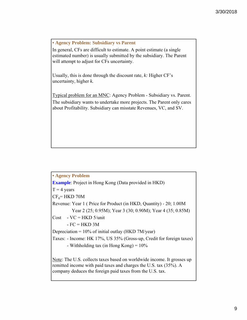
• Agency Problem: Subsidiary vs Parent
In general, CFs are difficult to estimate. A point estimate (a single estimated number) is usually submitted by the subsidiary. The Parent will attempt to adjust for CFs uncertainty.
Usually, this is done through the discount rate, k: Higher CF’s uncertainty, higher k.
Typical problem for an MNC: Agency Problem - Subsidiary vs. Parent.
The subsidiary wants to undertake more projects. The Parent only cares about Profitability. Subsidiary can misstate Revenues, VC, and SV.
• Agency Problem
Example: Project in Hong Kong (Data provided in HKD)
T = 4 years
CF0= HKD 70M
Revenue: Year 1 ( Price for Product (in HKD, Quantity) - 20; 1.00M
Year 2 (25; 0.95M); Year 3 (30; 0.90M); Year 4 (35; 0.85M)
Cost - VC = HKD 5/unit
- FC = HKD 3M
Depreciation = 10% of initial outlay (HKD 7M/year)
Taxes: - Income: HK 17%, US 35% (Gross-up, Credit for foreign taxes)
- Withholding tax (in Hong Kong) = 10%
Note: The U.S. collects taxes based on worldwide income. It grosses up remitted income with paid taxes and charges the U.S. tax (35%). A company deduces the foreign paid taxes from the U.S. tax.

3/30/2018
10
Example (continuation):
St = 7 HKD/USD (use RW to forecast future St’s)
SV4 = HKD 25M
k = 15%
1. Subsidiary’s NPV (in HKD including local taxes)
T=1 2 3 4
Revenues 20M 23.75M 27M 29.75M
Cost 5M 4.75M 4.5M 4.25M
3M 3M 3M 3M
Profit 12M 16M 19.5M 22.5M
Dep. 7M 7M 7M 7M
EBT 5M 9M 12.5M 15.5M
Taxes .85M 1.53M 2.125M 2.635M
EAT 4.15M 7.47M 10.375M 12.865M
Free CFs 11.15M 14.47M 17.375M 19.865M
Example: (continuation)
T=1 2 3 4
Free CF +SV 11.15M 14.47M 17.375M 44.865M
NPV (in HKD) = -70M + 11.15M/1.15 + 14.47M/1.152 + + 17.375M/1.153 + 44.865M/1.154 = - HKD 12.2869M <0
Note: If SV4 is changed to HKD 80M, then NPV = 19.16M >0!
Subsidiary would submit the project.
(This is likely to happen: The subsidiary will never submit a project to the parent company with a NPV<0.) Thus, SV is very important!

3/30/2018
11
Year 1 Year 2 Year 3 Year 4
CFs to be remitted (HKD)
11.15M 14.47M 17.375M 19.865M+25M
St = 7 HKD/USD
CFs in USD 1.59M 2.067M 2.48M 2.84M+3.57MWithholding (.159M) (.2067M) (.248M) (.284M)CFs remitted 1.431M 1.86M 2.3M 2.56M+3.57M(US Tax) (.6M) (.8M) (.975M) (1.125M)Tax Credit .281M .425M .552M .376MNet Tax (.319M) (.425M) (.423M) (.749M)EAT 1.114M 1.486M 1.811 2.09M+3.57M
2. MNC’s NPV (in USD, including all taxes)
NPV = - USD 10M + 6.5195M = - USD 3.48M < 0. => No!
Note: A subsidiary will never submit a project like this (they want to undertake the project.) A subsidiary will inflate some numbers, for example, SVT.
If SVT = HKD 80M, then
NPV (USD M)=10–{1.114/1.15 +1.486/1.152 +1.811/1.153
+(2.095+80/7)/1.154} = USD 1.01181 M > 0 Yes. 
3/30/2018
12
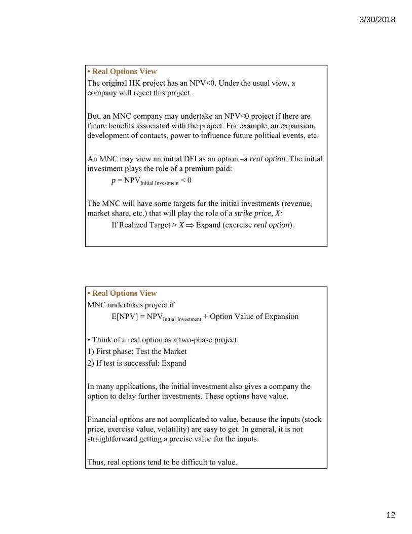
• Real Options View
The original HK project has an NPV<0. Under the usual view, a company will reject this project.
But, an MNC company may undertake an NPV<0 project if there are future benefits associated with the project. For example, an expansion, development of contacts, power to influence future political events, etc.
An MNC may view an initial DFI as an option –a real option. The initial investment plays the role of a premium paid:
p = NPVInitial Investment < 0
The MNC will have some targets for the initial investments (revenue, market share, etc.) that will play the role of a strike price, X:
If Realized Target > X Expand (exercise real option).
• Real Options View
MNC undertakes project if
E[NPV] = NPVInitial Investment + Option Value of Expansion
• Think of a real option as a two-phase project:
1) First phase: Test the Market
2) If test is successful: Expand
In many applications, the initial investment also gives a company the option to delay further investments. These options have value.
Financial options are not complicated to value, because the inputs (stock price, exercise value, volatility) are easy to get. In general, it is not straightforward getting a precise value for the inputs.
Thus, real options tend to be difficult to value.

3/30/2018
13
Example: Malouf Coffee considers expanding to Mexico by opening 2 stores: S & B. If the expansion is done simultaneously, the upfront investment is 230. There is a 70% probability of failure (F) & k=.15:
CFs for S: 60 (if F) & 140 (if not F)
CFs for B: 120 (if F) & 280 (if not F).
E[NPV] = -230 + [(.70)*(60+120) + (.30)*(140+280)]/1.15 = -10.87 <0.
CFs for a 2-phase expansion (1st S; 2nd B), with Initial Investment = 100& Expansion Investment = 70 if X (CFs) > 120. With P1=.70 & P2=.50; & k=.15 (Learning: Lower expansion investment & lower P2):
P1
P2
1- P1
1- P2
60
120
140
280
E[NPV1st-phase ] = -100 + [(.70)*60 + (.30)*140]/1.15 = -26.96<0 No!
Example (continuation): If we evaluate the 2-phase investment, we get:
E[NPV] = -100 + (.70)*60/1.15 + (.30)*{(140-70)/1.15 +
[(120)*.50+(280)*.50]/1.152} = 0.1512 > 0 YES!
Much higher valuation when real option (flexibility) is introduced.
Technical Note: The discount rate in the 2nd-phase should be lower! 
• In general, not easy to determine P1 & P2 and future CFs.
• Value of the Real Option: The firm learns from 1st-phase & adapts the behavior (expand, delay, or close the project). It limits the downside.
• Many MNCs went to China in the early 1990s with NPV<0 projects. Years later, some expanded (BMW, Nike, Starbucks), while others closed the projects and left the market (Home Depot, Mattel).

3/30/2018
14
• Adjusting Project Risk
MNCs use different techniques to adjust for uncertainty in the estimated CFs submitted by the subsidiaries.
• Adjusting discount rate, k
In general, CF’s uncertainty is incorporated in the evaluation process through the discount rate, k: The higher the uncertainty, the higher k.
In general, k incorporates economic and political uncertainty in the local country.
But k is a point estimate, an average risk. Using an average risk, may cost an MNC: It may wrongly reject (accept) projects that have a below (above) average risk.
Sometimes, it is better to use a range instead for k, say {kLB, kUB}.
Sometimes, it is better to use a range instead for k, say {kLB, kUB} to create a range for {NPV(kLB), NPV(kUB)}.
Example: A range for NPV based on {kLB, kUB} for the HK project.
Suppose the Parent decides to build a range for NPVs based on {kLB=.135, kUB=.165} (using SV4 = HKD 80M to get NPV>0):
Range for NPV: {USD 0.535M; USD 1.519M}. 

3/30/2018
15
• Sensitivity Analysis/Simulation
Subsidiaries may not be forthcoming about true profitability of projects. MNCs will use sensitivity analysis to study the subsidiaries’ proposals.
1) Sensitivity Analysis of the impact of CFs on the NPV of project
⋄ Play with different scenarios/Simulation
Steps: a. Assign a probability to each scenario
b. Get an NPV for each scenario.
c. Calculate a weighted average (weight=probability) NPV E[NPV]
d. If possible, use a risk-reward measure (say, a Sharpe Ratio).
⋄ Breakeven Analysis (same as what we do below for SV).
• Sensitivity Analysis/Simulation
Example: Scenarios for CFs and E[NPV] & SD[NPV] for HK project
We create different scenarios for the CFs (as a % of submitted CFs)
% of CFs Probability NPV (in M)0.60 0.01 -0.779180.64 0.025 -0.600090.68 0.05 -0.420990.72 0.075 -0.241890.76 0.09 -0.062790.80 0.10 0.1163130.84 0.125 0.2954120.88 0.15 0.4745120.92 0.15 0.6536110.96 0.125 0.832711
1 0.10 1.01181
E[NPV] 0.35541SD[NPV] 0.64477Prob[NPV<0] 0.25

3/30/2018
16
• Sensitivity Analysis/Simulation
• Descriptive StatsE[NPV] = USD 0.355411 MSD[NPV] = USD 0.644769 MProb[NPV<0] = 0.250000SR= E[]/SD[] = 0.55122195% C.I. (Normal): (-0.90834M; 1.61916M)
• Sensitivity Analysis/Simulation - Decisions
A Parent can base a decision using some risk-reward rule. For example, a firm may look at the SR (using E[NPV] and SD[NPV]), the range –i.e., the difference between best and worst case scenarios-, establishing some ad-hoc tolerable level for the probability of negative NPV, etc.
• Decisions
Rule: Among the projects with E[NPV]>0, the Parent will compare the SRs (or CIs) for different projects and select the project with the higher SR (or the CI with the smallest negative part). 
3/30/2018
17
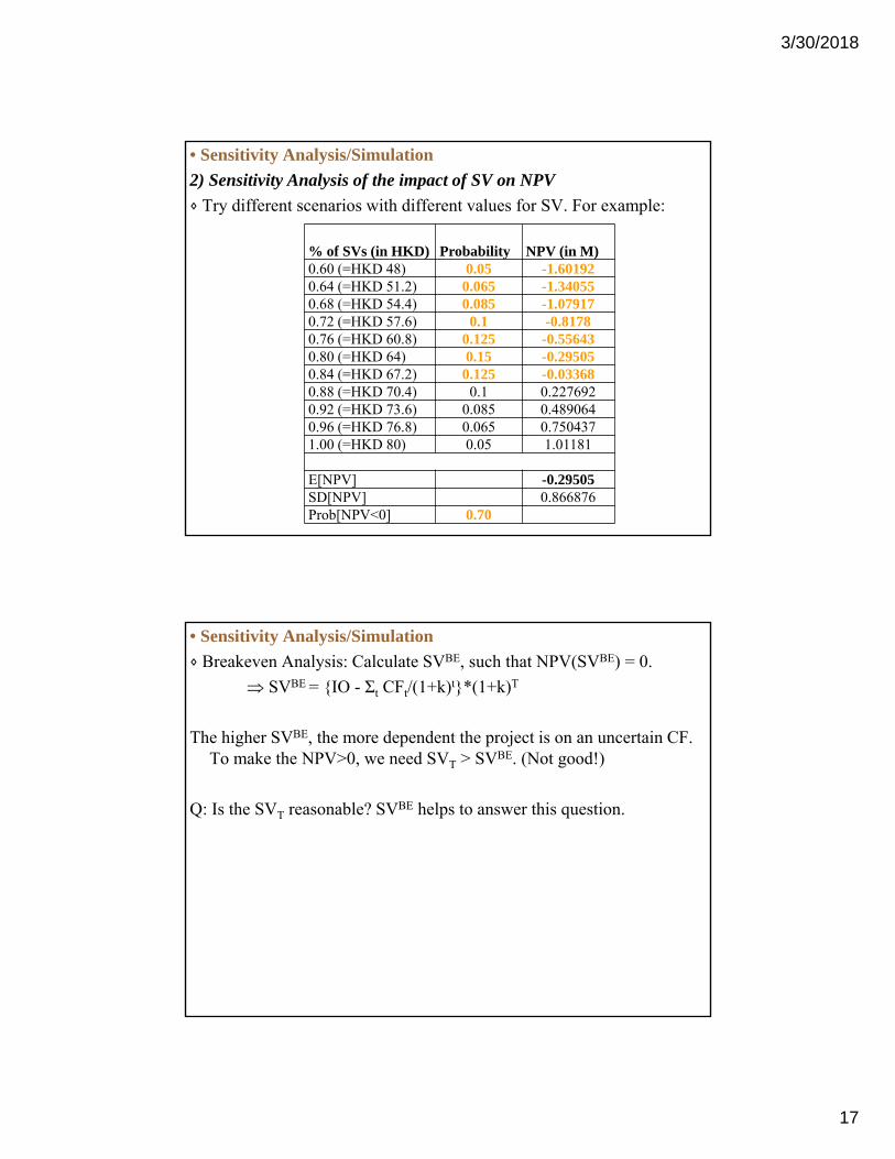
• Sensitivity Analysis/Simulation
2) Sensitivity Analysis of the impact of SV on NPV
⋄ Try different scenarios with different values for SV. For example:
% of SVs (in HKD) Probability NPV (in M)0.60 (=HKD 48) 0.05 -1.601920.64 (=HKD 51.2) 0.065 -1.340550.68 (=HKD 54.4) 0.085 -1.079170.72 (=HKD 57.6) 0.1 -0.81780.76 (=HKD 60.8) 0.125 -0.556430.80 (=HKD 64) 0.15 -0.295050.84 (=HKD 67.2) 0.125 -0.033680.88 (=HKD 70.4) 0.1 0.2276920.92 (=HKD 73.6) 0.085 0.4890640.96 (=HKD 76.8) 0.065 0.7504371.00 (=HKD 80) 0.05 1.01181
E[NPV] -0.29505SD[NPV] 0.866876Prob[NPV<0] 0.70
• Sensitivity Analysis/Simulation
⋄ Breakeven Analysis: Calculate SVBE, such that NPV(SVBE) = 0.
SVBE = {IO - Σt CFt/(1+k)t}*(1+k)T
The higher SVBE, the more dependent the project is on an uncertain CF. To make the NPV>0, we need SVT > SVBE. (Not good!)
Q: Is the SVT reasonable? SVBE helps to answer this question.

3/30/2018
18
Example: Calculate SVBE for HK project.
SVBE = {10M - {1.114M/1.15 + 1.486M/1.152 + 1.811M/1.153 +
+ 2.09M/1.154}*1.154 = USD 9.65891 (or HKD 67.61236M)
Check:
NPV(USD M) = 10 – {1.114/1.15 + 1.486/1.152 + 1.811/1.153 +
+ (2.09+67.61236/7)/1.154}= 0
A parent company compares the SVBE with the reported SV value:
SVBE = HKD 67.61236M < SV4 = HKD 80M. (Too big!) 
Note: If SVBE is negative, it is good for the evaluation of the project. Itsprofitability does not depend at all on an uncertain –and difficult toestimate- future CF.
• Judgment call
We presented several techniques that can be used by an MNC to measure and evaluate a project’s risk. But, in practice there is a lot of subjective judgment.
MNCs also incorporate their own and/or a consultant’s experience to make a decision. Introducing a judgment call in the process is acceptable, given that in building scenarios, changing k, assuming distributions, experience also plays a very important role.
Example: Ad-hoc decision
Based on past experience, the Parent not only requires E[NPV]>0, but as an additional control for risk that Prob[NPV<0] be lower than 30%. In the HK example, the probability of a negative NPV is 25%, which would be acceptable under this ad-hoc risk-reward rule.
Note: This ad-hoc rule double counts risk, since NPV is calculated using risk-adjusted discount rates! 

3/30/2018
19
II.3 Capital Structure and Cost of Capital
• Cost of Capital
Firms use the cost of capital as the discount rate for CFs. In this section want to answer the following question:
Q: How do MNCs set discount rates for projects in foreign countries?
• From Chapter IX, we know that Country Risk affects discount rates and, thus, projects:
- Because of CR, different countries have different risk free rates (kf).
- High CR, high risk kf.
• The cost of capital depends on the debt-equity mix of a firms & the nature (diversified firm/diversified ownership) of the firm.
• Brief Review: Capital Structure
• A firm can raise new capital by:
- Issuing new equity (E) –a firm gives away ownership; pays dividends
- Issuing debt (D) –a firm borrows; pays interest.
A firm can also use retained earnings, which we will consider E. (According to the pecking order theory, retained earnings are the first source of funds for a company.)
• Trade-off Theory of Capital Structure
- Debt has its (tax) advantages (reduces taxes), but also its disadvantages (cost: bankruptcy).
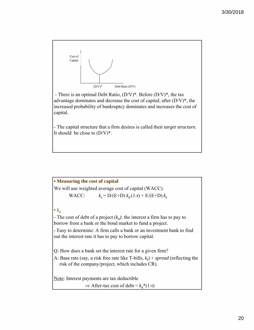
- Firms will use the E & D mix that minimizes the cost of capital. There is a U-shape relation between cost of capital and the amount of debt relative to the total value of the firm (V=E+D).
3/30/2018
20
- There is an optimal Debt Ratio, (D/V)*. Before (D/V)*, the tax advantage dominates and decrease the cost of capital; after (D/V)*, the increased probability of bankruptcy dominates and increases the cost of capital.
- The capital structure that a firm desires is called their target structure. It should be close to (D/V)*.
Cost of Capital
Debt Ratio (D/V)(D/V)*
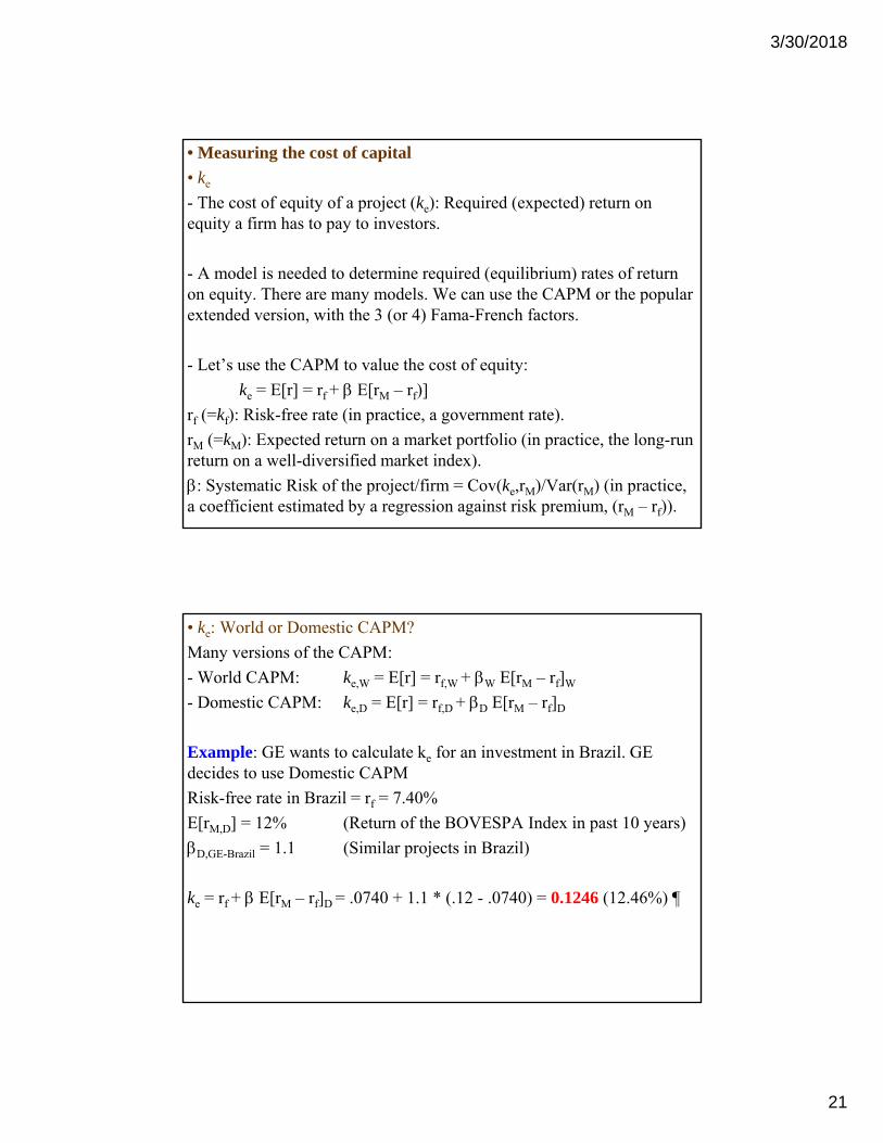
• Measuring the cost of capital
We will use weighted average cost of capital (WACC).
WACC: kc = D/(E+D) kd (1-t) + E/(E+D) ke
• kd
- The cost of debt of a project (kd): the interest a firm has to pay to borrow from a bank or the bond market to fund a project.
- Easy to determine: A firm calls a bank or an investment bank to find out the interest rate it has to pay to borrow capital.
Q: How does a bank set the interest rate for a given firm?
A: Base rate (say, a risk free rate like T-bills, kf) + spread (reflecting the risk of the company/project, which includes CR).
Note: Interest payments are tax deductible
After-tax cost of debt = kd*(1-t)
3/30/2018
21
• Measuring the cost of capital
• ke
- The cost of equity of a project (ke): Required (expected) return on equity a firm has to pay to investors.
- A model is needed to determine required (equilibrium) rates of return on equity. There are many models. We can use the CAPM or the popular extended version, with the 3 (or 4) Fama-French factors.
- Let’s use the CAPM to value the cost of equity:
ke = E[r] = rf + E[rM – rf)]
rf (=kf): Risk-free rate (in practice, a government rate).
rM (=kM): Expected return on a market portfolio (in practice, the long-run return on a well-diversified market index).
: Systematic Risk of the project/firm = Cov(ke,rM)/Var(rM) (in practice, a coefficient estimated by a regression against risk premium, (rM – rf)).
• ke: World or Domestic CAPM?
Many versions of the CAPM:
- World CAPM: ke,W = E[r] = rf,W + W E[rM – rf]W
- Domestic CAPM: ke,D = E[r] = rf,D + D E[rM – rf]D
Example: GE wants to calculate ke for an investment in Brazil. GE decides to use Domestic CAPM
Risk-free rate in Brazil = rf = 7.40%
E[rM,D] = 12% (Return of the BOVESPA Index in past 10 years)
D,GE-Brazil = 1.1 (Similar projects in Brazil)
ke = rf + E[rM – rf]D = .0740 + 1.1 * (.12 - .0740) = 0.1246 (12.46%) 

3/30/2018
22
• ke: World or Domestic CAPM?
Many versions of the CAPM:
- World CAPM: ke,W = E[r] = rf,W + W E[rM – rf]W
- Domestic CAPM: ke,D = E[r] = rf,D + D E[rM – rf]D
Q: Which one should be used?
A: In theory, it depends on the view that a company has regarding capital markets or what compensation expect/demand shareholders.
- If capital markets are integrated (or shareholders are worldwide diversified) use World benchmark (say, MSCI World Index).
- If capital markets are segmented (or shareholders hold domestic portfolios) use Domestic benchmark (say, Bovespa Index in Brazil).
E[rM – rf]W driven by world factors (world benchmark used)
E[rM – rf]D driven by domestic factors (domestic benchmark used)
• ke: World or Domestic CAPM?
The difference between both models can be significant:
- 5.55% absolute difference in EM
- 3.58% absolute difference in Developed Markets (DM).
- W & D also show significant absolute differences: 0.44 for EM & 0.21 for DM.
The evidence for integrated capital markets is weak. We tend to think of capital markets as partially integrated. Then:
- Partially Integrated CAPM: ke = wD ke,D* + (1- wD) ke,w
where,
ke,D*: FC-adjusted domestic cost of capital ke,D (both ke in same currency)
wD: Measure of weight of Domestic Market in world capital markets.
Note: Similar ideas can be extended to 3- or 4-factor Fama-French models.

3/30/2018
23
In general, we find that World CAPM produces low expected returns.
The Fama-French 3-factor model tends to produce higher (and more realistic) expected returns.
Many ad-hoc adjustments are used in the private sector. For example, estimate World CAPM and add a CR premium (sovereign yield spread).
Example: Cost of capital Adjustment for project in Brazil
E(rM – rf)US = 3.45%
βW = 0.8
CRBrazil = 2.80%
rf,US = 4.73%
ke = [.0473 + 0.8 * .0345] + .0280 = 10.29% (in USD) 
Details behind WACC:
WACC: kc = D/(E+D) kd (1-t) + E/(E+D) ke
⋄ Dividends are not tax deductible. There is an advantage to using debt!
⋄ Time-consistency between ke & kd. The same maturity should be used for ke and kd. That is, if you use long-term bonds to calculate kd , you should also use long-term bonds to calculate ke.
⋄ In Chapter IX we discussed country risk. For practical purposes, many emerging market governments bonds may not be considered risk-free. Thus, the government bond rate includes a default spread, which, in theory, should be subtracted to get rf.
⋄ is estimated by the slope of a regression against a market index. There are many issues associated with the estimation of : choice of index, noisy data, adjustment by leverage, mean reversion, etc.
3/30/2018
24
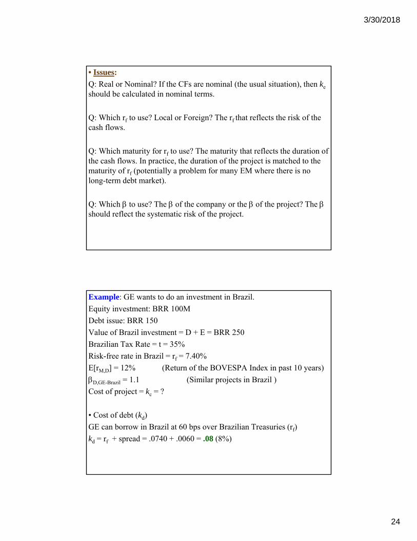
• Issues:
Q: Real or Nominal? If the CFs are nominal (the usual situation), then ke
should be calculated in nominal terms.
Q: Which rf to use? Local or Foreign? The rf that reflects the risk of the cash flows.
Q: Which maturity for rf to use? The maturity that reflects the duration of the cash flows. In practice, the duration of the project is matched to the maturity of rf (potentially a problem for many EM where there is no long-term debt market).
Q: Which to use? The of the company or the of the project? The should reflect the systematic risk of the project.
Example: GE wants to do an investment in Brazil.
Equity investment: BRR 100M
Debt issue: BRR 150
Value of Brazil investment = D + E = BRR 250
Brazilian Tax Rate = t = 35%
Risk-free rate in Brazil = rf = 7.40%
E[rM,D] = 12% (Return of the BOVESPA Index in past 10 years)
D,GE-Brazil = 1.1 (Similar projects in Brazil )
Cost of project = kc = ?
• Cost of debt (kd)
GE can borrow in Brazil at 60 bps over Brazilian Treasuries (rf)
kd = rf + spread = .0740 + .0060 = .08 (8%)

3/30/2018
25
• Cost of debt (kd)
kd = rf + spread = .0740 + .0060 = .08 (8%)
• Cost of equity (ke)
GE decides to use Domestic CAPM
ke = rf + E(rm – rf) = .0740 + 1.1 * (.12 - .0740) = 0.1246 (12.46%)
• Cost of Capital –WACC– (kc)
kc = D/(E+D) kd (1-t) + E/(E+D) ke
kc = (.60) * .08 * (.65) + (.40) * 0.1246 = .08104 (8.104%)
Note: This is the discount rate that GE should use to discount the cash flows of the Brazilian project. That is, GE will require an 8.104% rate of return on the investment in Brazil. 
Remark: When kc ↑ NPV of projects ↓.
That is, anything that affects kc, also affects the profitability (NPV) of a project.
Application: Argentina defaults in some of its debt.
Argentina’s CR ↑ rf,Arg ↑ & kc,Arg ↑.
Some projects in Argentina become negative NPV projects.
MNCs may suddenly abandon Argentine projects.

3/30/2018
26
Estimating E[rM - rf]:
ERP premiums are estimated with error. To minimize this problem, we use as many years as possible to build the long-run average. Remember that using averages comes with an associated standard error:
More data lower S.E. -i.e., more precision.
But, even with more than 100 years of data for developed markets there is no consensus on an ERP (& how to estimate it). For the U.S. market, Duarte and Rosa (2015) list over 20 different approaches to estimate the ERP in the U.S.
Using data from 1960 to 2013, Duarte and Rosa (2015) report estimates from -0.4% to 13.1%, with a 5.7% average for all model. A wide range!
Table X.4 reports estimates from 0.79% (Italy) to 12.06 (HK), using the average U.S. T-Bill rate for the period (≈4.7%)
Estimating E[rM - rf]: From Duarte and Rosa (2015), wide range:

3/30/2018
27
Estimating E[rM - rf]: The international evidence (wide range too!)
Market Equity Return
Standard Deviation
ERP
U.S. 8.19 15.04 0.0345Canada 8.22 19.35 0.0349France 9.02 22.17 0.0427Germany 9.37 21.67 0.0462Italy 5.08 25.38 0.0079Switzerland 10.44 17.83 0.0567U.K. 7.77 21.44 0.0302Japan 9.94 20.74 0.0520Hong Kong 16.80 33.72 0.1206Singapore 12.26 27.79 0.0752Australia 7.68 23.79 0.0293
World 7.70 14.58 0.0295EAFE 8.00 16.78 0.0326
Table X.4MSCI Index USD Equity Returns and ERP: (1970-2017)
Estimating E[rM - rf]:
• Lack of long history and quality data may be a problem for EM.
• For these markets, say Country J, it is sometimes easier to adjust the ERP from a well-established, mature market, say, the U.S., to estimate the ERPJ. Several ways to do this adjustment:
⋄ Relative Equity Market Approach:
The U.S. risk premium is modified by the volatility of the Country J’s equity market, σJ, relative to the volatility of the U.S equity market, σUS:
E[rM – rf]J = E[rM – rf]US * σJ/ σUS
(Potential problem: σJ is also an indicator of liquidity!)
3/30/2018
28
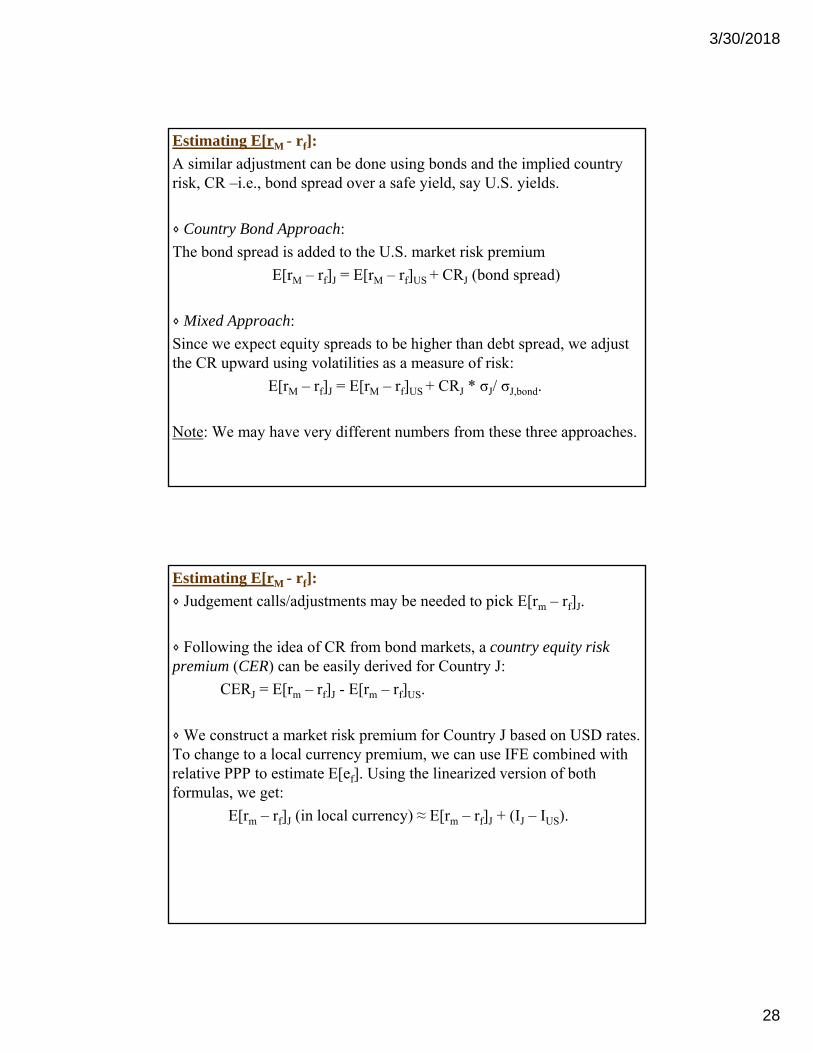
Estimating E[rM - rf]:
A similar adjustment can be done using bonds and the implied country risk, CR –i.e., bond spread over a safe yield, say U.S. yields.
⋄ Country Bond Approach:
The bond spread is added to the U.S. market risk premium
E[rM – rf]J = E[rM – rf]US + CRJ (bond spread)
⋄ Mixed Approach:
Since we expect equity spreads to be higher than debt spread, we adjust the CR upward using volatilities as a measure of risk:
E[rM – rf]J = E[rM – rf]US + CRJ * σJ/ σJ,bond.
Note: We may have very different numbers from these three approaches.
Estimating E[rM - rf]:
⋄ Judgement calls/adjustments may be needed to pick E[rm – rf]J.
⋄ Following the idea of CR from bond markets, a country equity risk premium (CER) can be easily derived for Country J:
CERJ = E[rm – rf]J - E[rm – rf]US.
⋄ We construct a market risk premium for Country J based on USD rates. To change to a local currency premium, we can use IFE combined with relative PPP to estimate E[ef]. Using the linearized version of both formulas, we get:
E[rm – rf]J (in local currency) ≈ E[rm – rf]J + (IJ – IUS).

3/30/2018
29
Example: GE’s wants to adjust (rM – rf)Brazil using different methods, using the U.S. as a benchmark. GE uses the following data:
E[rM – rf]US = 3.45% (rf,US = 4.73%)
σUS = 15.2%
σBrazil = 37.3% (based on past 15 years)
σBrazil,bond = 23.1% (based on past 15 years)
CRBrazil = 2.80%
⋄ Relative Equity Market Approach:
E[rM – rf]Brazil = .0345 * .373/.152 = 0.08466
ke,Brazil = rf + E[rM – rf]Brazil = .0473 + 1.1 * 0.08466 = 0.1404.
⋄ Mixed Approach:
E[rM – rf]Brazil = .0345 + .028 *.373/.231 = 0.07971
ke,Brazil = rf + E[rM – rf]Brazil = .0473 + 1.1 *0.07971 = 0.1350.
Example (continuation): Suppose GE decides to use the Relative Equity Market Approach. Now, GE wants to translate the cost of capital in USD to BRL, using linearized PPP.
Data for average inflation rates:
E[IBrazil] = 7.5%
E[IUS] = 3%
⋄ Relative Equity Market Approach:
E[rM – rf]Brazil = .0345 * .373/.152 = 0.08466
E[rm – rf]Brazil (in BRL) ≈ 0.08466 + (0.075-0.03) = 0.12966. 

3/30/2018
30
• Target Debt-Equity Ratio in Practice
Suppose that GE’s target debt-equity ratio is 70%-30%. It is unlikely that GE will raise funds with a 70-30 debt-equity split for every project. For example, for the Brazilian project, GE is using a 60-40 D/E split.
The target (D/V)* reflects an average; it is not a hard target for each project. That is, for other projects GE will use D/E to compensate and be close to the (D/V)*.
Determinants of Cost of Capital for MNCs
Intuition: Economic factors that make the CFs of a firm more stable reduce the kc.
1) Size of Firm (larger firms get better rates from creditors and have lower s)
2) Access to international markets (better access, more chances of finding lower rates)
3) Diversification (more diversification, more stable CFs, lower rates. Also, s closer to M)
4) Fixed costs (the higher the proportion of fixed costs, the higher the )
5) Type of firm (cyclical companies have higher s)
6) FX exposure (more exposure, less stable CFs, worse rates)
7) Exposure to CR (again, more exposure to CR, less stable CFs, worse rates).

3/30/2018
31
Example: Cost of Capital (Nov 2014):
General Electric (GE): Huge, internationally diversified company
Disney (DIS): Large, moderate degree of international diversification
The GAP (GPS): Medium cap, low international diversification.
US Treasuries (kf): 1.63% (5-year T-bill rate, from Bloomberg)
S&P 500 return (E[rm]): 8.433% (30 years: 1984-2014, from Yahoo)
tax rate (t): 27.9% (effective U.S. tax rate, according to World Bank)
Recall: kc = D/(E+D) kd (1-t) + E/(E+D) ke
E D Rating Spread kd ke WACC
GE 135B 313B AA- 27 1.24 1.90 10.07 3.99
DIS 45.5B 16.1B A+ 30 0.96 1.93 8.16 6.39
GPS 3B 1.4B BBB- 168 1.65 3.31 12.86 9.53