jkIalexandria.tue.nl/openaccess/Metis235417.pdfjkI I (b) Fig. 1. (a) Sequence containing a burst of...

IEEE TRANSACTIONS ON ACOUSTICS, SPEECH. AND SIGNAL PROCESSING, VOL. ASSP-34, NO. 2, APRIL 1986 317

Adaptive Interpolation of Discrete-Time Signals That Can Be Modeled as Autoregressive Processes I A. J. E. M. JANSSEN, RAYMOND N. J. VELDHUIS,, AND LODEWIJK B. VRIES

Abstract-This paper presents an adaptive algorithm for the restoration of lost sample values in discrete-time signals that can locally be

are that the positions of the unknown samples should be known and that they should be embedded in a sufficiently large neighborhood of known samples. The estimates of the unknown samples are obtained by minimizing the sum of squares of the residual errors that involve estimates of the autoregressive parameters. A statistical analysis shows that, for a burst of lost samples, the expected quadratic interpolation error per sample converges to the signal variance when the burst length tends to infinity. The method is in fact the first step of an iterative algorithm, in which in each iteration step the current estimates of the missing samples are used to compute the new estimates. Furthermore, the feasibility of implementation in hardware for real-time use is es- tablished. The method has been tested on artificially generated autoregressive processes as well as on digitized music and speech signals.

described by means of autoregressive processes. The only restrictions sk t

T I . INTRODUCTION

HIS paper treats the problem of restoring (or interpolating) unknown or lost sample values in a discrete-

time signal. An algorithm is presented that is capable of restoring satisfactorily unknown samples with known positions occurring in bursts and more general patterns. Ex- amples of both cases are shown in Fig. 1. To restore the unknown samples, the algorithm uses the information contained in the known neighboring samples.

Until rather recently, the problem of estimating unknown sample values in discrete-time signals in real time could only be solved by relatively simple, nonadaptive methods, such as Lagrange-type curve fitting. These methods are not well suited for signals primarily containing harmonic components, especially not when the number of samples in the periods of the harmonic components is less than the number of unknown samples. For instance, linear interpolation gives already audible interpolation errors for bursts in digital audio signals of length 5 . Because of the progress made in the field of chip design, one can now contemplate more complicated real- time restoration methods that may also involve some signal model. An example of such a method, where no model is assumed, can be found in [l]. This (adaptive) method deals with restoring discrete-time signals of which every' nth sample.is unknown. Examples of methods that inter- polate under certain model assumptions have been given

Manuscript received March 2, 1984; revised September 9, 1985. The authors are with the Philips Research Laboratories, 5600 JA Eind-

IEEE Log Number 8406769. hoven, The Netherlands.

I

jkI

I (b)

Fig. 1. (a) Sequence containing a burst of unknown samples. (b) Sequence containing a random pattern of unknown samples. ,

in [2, Section 111 and in [3]. Reference [2], in which the assumed model is an autoregressive process, deals with the restoration of a single unknown sample by minimizing the expected quadratic interpolation error. The assumed model in [3] is band-limitedness of the signals to a baseband which is a fraction of the sample frequency. In this nonadaptive method, analyzed in [3] for burst errors, the restoration is done in such a way that the restored signal has minimal energy outside the prescribed baseband. Un- fortunately, the latter method is very sensitive to the presence of noise and of out-of-band components in the sig-

0096-3518/86/0400-0317$01 .OO 0 1986 IEEE .

Authorized licensed use limited to: Eindhoven University of Technology. Downloaded on March 03,2010 at 09:25:49 EST from IEEE Xplore. Restrictions apply.

318 IEEE TRANSACTIONS ON ACOUSTICS, SPEECH, AND SIGNAL PROCESSING, VOL. ASSP-34. NO. 2, APRIL 1986

nal, even when the number of lost samples is small and the spectral energy of the signal is well within the baseband.

In this paper, the same point of view as in [Z, Section 111 is taken for the restoration of more general patterns of unknown samples than single ones or bursts. That is, it is assumed that the signals to be interpolated can be modeled as autoregressive (AR) processes of finite order. The restoration is done in such a way that the restored signal fits the assumed model as well as possible.

The method is adaptive in the sense that, from a finite segment of data, one first has to estimate the AR parameters. Once these are known, the unknown samples can be obtained as the solutions of a system of linear equations. In fact, the AR parameters as well as the unknown samples could be obtained in one step by minimizing some function involving both AR parameters and unknown samples. However, this function contains fourth-order terms and minimizing it is a nontrivial problem. Here a suboptimal approach is adopted, where first the parameters are estimated from the incomplete data and next the unknown samples. This can be considered to be the first step of a rapidly converging iterative minimization procedure. This procedure will be discussed in an appendix.

The choice of the autoregressive process as a model for the signal can be motivated by the fact that many signals that are encountered in practice can be modeled in this way. Therefore, it is expected that the interpolation method presented here can be applied successfully in many practical situations. For instance, as will be dem- onstrated further on, good results are obtained for the interpolation of digitized music and speech signals.

The organization of this paper is as follows. In Section 11, the interpolation method is presented and a statistical analysis is given. The interpolation error is analyzed under the assumption that the AR parameters are known; this analysis is detailed for the case that Gaussian probability density functions are assumed. In Section 111, efficient methods for the approximate calculation of AR parameters and unknown samples are given. Also, the numerical properties of certain parts of the algorithm are discussed. In Section IV, some results are presented. Here a comparison of performance to other methods is given. Section V presents some conclusions. Finally, the paper contains a number of appendixes to which proofs not relevant to the main text and much of the mathematics are deferred.

11. PRESENTATION AND ANALYSIS OF THE INTERPOLATION METHOD

In this section, it is assumed that sk , k = - 03, . . . , 03, is a realization of a stationary autoregressive process

is a stochastic variable). This means that there exist a finite positive integer p , the prediction order, numbers ao, a l , * , up, .ao = 1 , the prediction coefficients, and a zero-mean white noise process E k , k = - 03, . . . , 03, the excitation noise, with variance af, such that

$k, k = -03, * * * , 03 (the tilda - indicates that a variable

UOSk + U l 5 - l + - + U,.Tk-_, = Z k ,

k = - 00, 2 O3. (11.1)

For notational convenience, it shall be agreed that ak = 0 for k < 0 or k > p . The AR spectrum S ( 0 ) of fk, k = -03, . . * , 03, is given by

where

(11.3)

In Section 11-A, the algorithm for estimating the AR parameters and the unknown samples from a finite sequence of samples is presented. A statistical analysis of the interpolation error is given in 11-B.

A . Presentation of the Interpolation Method The available data consist of a segment sk, k = 0, * - * ,

N - 1, of a realization of an AR process &, k = - 0 3 ,

ples occur at the known time instants t ( l ) , - * * 2 t ( m ) , where0 < p I t ( 1 ) < < t ( m ) 5 N - p - 1 . The problem is to estimate the values of the unknown samples - , up and a, from the available data in such a way that the restored segment fits the assumed model as well as possible in a quadratic sense. That is, the restoration is such that the sum of the squares of the residual error ep, * - * , eN- I is minimal.

Although methods to estimate the order of an autoregressive process have been reported [4], it has been de- cided, if p is unknown, to choose p as a function of the number m of unknown samples. The rather arbitrary relation p = 3m + 2 has proved to give good interpolation results. For notational convenience, the vector notation a

Tdenotes vector or matrix transposition) shall be adopted. The estimation of a and x is expressed as a minimization problem, where the estimates d for a and P for x are chosen such that

. . . , 03. It is assumed throughout that the unknown sam-

y ) ? * * * , and the AR parameters p , a l ,

= [at, - . T , apl 3 x = [S,(I), * - * , st(,,JT (the superscript

N - 1 I P

is minimal as a function of a and x. Once d and R have been determined, a: is estimated by

(11.5)

The particular choice for minimizing Q ( a , x ) to obtain estimates for a and x is motivated by the following two facts. First, if s = [so, - , sN-I] and u = [so, - , sp - I ]T then, under the hypothesis that the sample values have a Gaussian probability density function, minimizing

T


JANSSEN et a / . : ADAPTIVE INTERPOLATION OF DISCRETE-TIME SIGNALS 319

Q(a, x) with respect to a turns out to be the same as maximizing the log likelihood function

L(a, 0 3 = 1% (Ps\r(SIU, a, 03) (11.6) as a function of a and 0:. This is a common procedure to estimate a and 0:. Second, also under the hypothesis that the sample values have a Gaussian probability density function, minimizing Q(a, x) with respect to x is the same as finding a minimum variance estimate for x, for known p and a. Both claims shall be proved in Appendix A.

Since Q(a, x) involves fourth-order terms, such as a?&), the minimization with respect to a and x is a non- tnvlal problem. Fortunately, one can often assume that the number m of unknown samples is small compared to the segment length N. A suboptimal approach can then be found as follows. One chooses an initial estimate f('), for instance, 2.') = 0, for the vector x of the unknown samples. Next, one minimizes Q(a, 2")) as a function of a to obtain an estimate 8. Finally, one minimizes Q(ci, x) as a function of x to obtain an estimate f for the unknown samples.

Both minimizations are feasible, since Q(a, x) is a quadratic form in both a E R p and x E R". In fact, it can be shown that

Q(a, x) = aTC(x) a + 2aTc(x) + cao(x). (11.7)

Here

C(x) = ( c g ( x ) ) i , j = I; ' , p ?

c(x> = [COI(X), * - 3 cop(x>lT, (11.8)

where N - I

cg(x) = s k - j s k - j , i , j = 0, 1, ' * 9 P. (11.9) k = p

Hence, C(x) is the p X p-autocovariance matrix, estimated from s k , k = 0, - - , N - 1. At the same time, it can be shown that

Q(a, x) = xTB(a)x + 2xTz(a) + D(a). (11.10)

Here

B(a) = (bt(i) - btu))i,j= I; . . ,rn,

z ( 4 = [ Z l ( 4 , * * * 9 Z " ( 4 I T I (11.11) bl, 1 -p, * . , p , has been defined in (11.3), and

P

zi(a) = b k s l ( i ) - k , i = 1, * * , m, (11.12) k = - p

and D(a) E RI depends on a and the known samples only. Hence, ci and 4 are given by

C(f ( 0 ) p = - c (2 ( O ) ) , (11.13)

and

B(ci)f = -~(ci), (11.14)

respectively. The above method for calculating prediction coefficients from a sequence of samples is known as the

autocovariance method [ 5 ] . On substitution of (11.13) into (11.5), it easily follows that

1 N - p - m

6; = (cm(f) + ciTc(f)). (11.15)

It should be noted at this point that the interpolation method just described can be considered as the first step of an iterative algorithm in which, in every step, new prediction coefficients ci are estimated as in (11; 13) by using, instead of f"), the previously estimated vector of sample values f obtained in (11.14). The prediction coefficients can be used again to obtain new estimates for the unknown samples and so on. It is clear that in this way Q(a, x) decreases to some nonnegative number. One may hope that the sequence thus obtained converges to a point where Q(a, x) attains its global minimum. Unfortunately, it seems very hard to prove any definite result in this direc- tion. However, it can be shown that this iterative minimization procedure closely resembles a maximum likelihood parameter estimation algorithm, well known in statistics: the EM algorithm [6]-[8]. The iterative version of the interpolation algorithm and its resemblance to the EM algorithm are discussed in Appendix B.

The interpolating vector f of (11.14) can also be obtained as the solution to a minimization problem in the frequency domain. Denote by s ( 0 ) the AR spectrum obtained by substituting 6: of (11.15) and ci of (11.13) into the expression for S(0) in (11.2). In Appendix A, it is proved that 4 of (11.14) minimizes, as a function of x E W", the integral

(11.16)

Here

1 N - p - l 2

s(e; x) = ___ - 2p 1 kzp sk exp (-Jek)l 7

--7F I e 5 n. (11.17)

Intuitively, by minimizing (I?. 16) with respect to the values of the unknown samples, one forces the restored signal to have little (much) spectral energy in those regions in the frequency domain where the estimated spectral energy is small (large). This brings out a relation with the interpolation method of [3], where the restoration is such that the spectral energy of the restored signal is concentrated as much as possible in the assumed baseband of the original signal. It should be noted that the integral in (11.16) can be related with the work of Itakura and Saito [9] on distortion measures for spectral densities.

B. Statistical Analysis of the Interpolation Error In this subsection, some statistical properties of the in-

terpolation error are discussed. It is assumed that p , a , and 0: are known. Since, in practice, these parameters are estimated from the data, this assumption may be a sim- plification from reality. However, it has the advantage that the results take a pleasant form.


320 IEEE TRANSACTIONS ON ACOUSTICS, SPEECH, AND SIGNAL PROCESSING, VOL. ASSP-34, NO. 2, APRIL 1986

The interpolation error is defined as the stochastic vector d,

d = d - x" = d + (B(u))-'&(a). (11.18)

Note that the realization z(aj of (11.14) is replaced by a stochastic vector z"(a). It follows easily from (11.18), and from the fact that E [ f k ] = 0 , that E [ d ] = 0 and that the estimator d is unbiased. The (stochastic) relative quadratic interpolation error per sample & is defined by

(11.19)

To evaluate the expectation E [e] of &, it is noted that

d = (B(a))-' (z"(a) + B(a)@ =: (B(aj)-' I?, (11.20)

and that fo r i = 1, * * 7 m, P P

bvj = c bk$r(i)-k = c a[&r,(;)+[ (11.21) k = -p l = O

as follows straightforwardly from the definitions in (11.3), (11.11 j , and (11.12). Thus,

E[ddT] = (B(u))-I E[GI?'] ( B ( u ) ) - l . (11.22)

Since (E[GG']ju = E [ ~ ; b v j ] = u&i)-r( i) , one has that E [ G G T ] = ofB(a) and that

E [dd'] = uf(B (a) ) - 1 . (11.23)

Finally, E[&?] is given by

For the expected relative quadratic interpolation error of the ith unknown sample, one has

E [ h 3 = u:((B(a))-1)i;7 i = 1, - * , m. (11.25)

The case of a burst of m consecutive unknown samples deserves somewhat more attention than the general case. Then the matrix B(a) is Toeplitz and therefore has some properties that facilitate a further analysis of the interpolation error. Toeplitz matrices are persymmetric: an rz X n-matrix M is persymmetric if Mv = M , + -j,n + I - i , i, j

that their inverses are also persymmetric. If B(aj is Toe- plitz then (B(a))-' is persymmetric, and

= 1, . . . , n. It is a property of persymmetric matrices

E [ d 3 = E[hi+I-i], i = 1, . . * , m. (11.26)

Extensive observations for the case of a burst of m unknown samples have revealed that the ((B(u))- ' )~~, i = 1,

large, and that the tend to have their maximum for i = m/2, i.e., in the middle of the burst. Hence, much of the error energy is usually concentrated in the middle of the burst.

In case of a burst, the asymptotic behavior of E [ & ] as m -+ 03 can be determined by applying the Szego limit theorem [lo]. From (11.24), one has

. . . , m, seem to depend quadratically on i for m not too

7 111

(11.27)

where hi is the ith eigenvalue of B ( a ) . According to the Szego limit theorem, one has, for any function F , contin- uous on the set {E{=-, bk exp (-jOk)jlOj < n],

1 lim - C F ( X J

m - m m j = l

Taking F ( a ) = & I , one finds by using (11.2),

I . ra7r

- - - 1 S(Oj de 1 1 - uf 2n -7r

(11.29)

Hence,

nz + m lim E[&] = 1. (11.30)

This shows that for long bursts of consecutive samples, the quadratic interpolation error per sample approaches the signal energy per sample.

The result (11.30) derived for the burst case is also useful for finding a bound on the interpolation error in the general case. Indeed, the matrix B(a) = (br,(i)-r(i))j,j= I , . . . , m is a principal submatrix of the ( t (m) - t(1) + 1) X ( t (m) - t(1) + 1) Toeplitz matrix B'(a) - ( b k - l ) k , [ = I , . . . , r (m) - r ( l ) + Denoting the first m eigenvalues of B (a) and B ' (a) in increasing order by A I , - - , h,, and X;, - , one has by [ 1 1, Section 3.5, Theo- rem5.61 that 0 < h/ < X i , i = 1, . , m. Hence,

-

m m

trace ( ( ~ ( a ) - ' ) = C X;' < C X/ - ' i = 1 i = I

< trace ((B'(U)-'), (11.31)

and it follows that E [ & ] is asymptotically bounded by limm-m sup rn-'(t(m) - t ( 1) + 1). Although this bound is not as good as for the burst case, the interpolation error in the case of m randomly positioned unknown samples usually turns out to be smaller than in the case of a burst of length m.

The interpolation error can be analyzed in some more detail if fi?k has a Gaussian probability density function. It then follows that d has a probability density function


JANSSEN et al.: ADAPTIVE INTERPOLATION OF DISCRETE-TIME SIGNALS 32 1

It is a rather tedious but straightforward exercise to cal-, culate the variance, var (2) = E [ ( J T J - E[dTd])2] , of 2:

4 *

var (E) = ___ (Je c x;! (11.33) mE[s":I2 i = I

In the case of a burst of unknown samples of length m, one can use the Szego limit theorem (11.28) with F(a) = C 2 . For large m, one finds

It can be observed that var (2) is larger if the signal spectrum S(0) is more peaky . 111. COMPUTATIONAL ASPECTS OF THE INTERPOLATION

ALGORITHM In this section, the computational aspects of the calcu-

lation of 6 in (11.13) and f in (11.14) are considered. It should be noted that a linear system needs to be solved for the calculation of both B and f. If p is chosen 3m + 2, which is done when p is unknown, the need for effi- ciency is more urgent for the calculation of ci than for the calculation o f f .

A. Calculation of the Prediction Coeficients The calculation of B in (11.13) is, in fact, a well-known

problem. It is often referred to as the autocovariance method and is discussed in great detail for instance in [5]. In this reference also, an efficient algorithm is given for solving B from (11.13) in O(p *) operations. It is the experience of the authors that an approximate calculation of ci also gives satisfactory interpolation 'results, so that other methods to calculate B can be applied too. An example of a different method to calculate & is the so-called autocorrelation method, where, instead of the system (11.13), the system R h = - r is solved. Here R = ((r(i - j)) i , j= . . . p is the p X p-autocorrelation matrix, r = [ r ( l ) , . * , r (p) lTand r ( j> = l/Nc;z$'-'sksk+Ijl,j = - P . " ' , p , is a (biased) estimate for the jth autocorrelation lag of S,, k = -GO, - - , 03. The system obtained in this way can also be solved in O(p2) operations by the Levinson-Durbin algorithm [ 121. As can be seen from the results presented in Section IV, in most cases there are no significant differences between the interpolation results obtained via the autocovariance method or via the autocorrelation method. In [5], a summary of the various methods to estimate 4 from a sequence of samples is given. The numerical stability of some of these methods is discussed in [13].

B. Calculation of the Unknown Samples For the calculation of f in (11.14), it makes sense to

analyze the matrix B ( d ) defined in (11.11) and (11.3) in some detail. It can be seen from (11.1 1) that B(6) has constant values bo on its main diagonal. Furthermore, the ma-

trix B(ci) is positive definite, as can be seen from the expression

which follows on inserting (11.11) and (11.3) into the left- hand side of (111.1). Indeed, when i ' is the largest index with ui, f 0, the term in the right-hand sum of (111.1) with k = -t(i ') equals u;! , as dl = 0 for 1 < 0, a. = 1 and ui = 0 for i > i '. Hence, if u has nonzero elements, the right-hand sum of (111.1) consists of nonnegative terms of which at least one is positive. This shows that B(B) is positive definite.

The fact that B(d) is positive definite allows one to use Cholesky decomposition [ 141 of B (6) for solving 2 from (11.14) in O(m3) operations. In case of a burst of unknown samples, B ( 6 ) is Toeplitz and (11.14) can be solved in O(m2) operations by the Levinson algorithm [ 151. Even in the case of a more general pattern of unknown samples, B ( d ) is related to a Toeplitz matrix, so that the system in (11.14) can be solved more efficiently by using generalized Levinson algorithms [ 161. However, this requires rather involved mathematics and does not lead to a less complicated hardware implementation, since the generalized Levinson algorithm to be used strongly depends on the pattern of unknown samples. For these reasons, in this paper, only the solution of 2 from (11.14) by using Cho- lesky decomposition is considered.

In a Cholesky decomposition, the matrix B(B) is decomposed as a product

B(B) = L L T (111.2)

or as a product

B(ci) = EDET. (111.3)

In (111.2), L is a lower triangular m X m-matrix, in (111.3) is a lower triangular m X m-matrix with constant values

1 on its main diagonal, D is a diagonal m X m-matrix

LLTf = -z(B) and B(B)f = LDET = -z(B) are now solved by subsequently solving by back substitution y and f,from L y = -z(B) and from = -z(h) , respectively, and 2 from LTf = y and ET%? = D - I f , respectively. Both forms of Cholesky decomposition take O(m3) operations. A drawback of the decomposition in (111.2) is that it requires the calculation of square roots. On the other hand, as is shown further on, the elements of L in (111.2) satisfy bounds that are more convenient if,one has a fixed point implementation in mind.

For the elements of the matrices L and D , one has the following results:

with D.. = L2. i = 1, * * 11 7 , m. The systems B(8)f =

1 5 L.. = D!:?? 5 bA'2, j = 1, . * JJ JJ , m, (111.4)

m

Li = bo, j = 1, 7 m, (111.5) i = 1


322 IEEE TRANSACTIONS ON ACOUSTICS, SPEECH, AND SIGNAL PROCESSING, VOL. ASSP-34, NO. 2, APRIL 1986

so that

I L , ( I (bo - i = 1, * * , j - 1,

j = 1, . * a 2 m. (111.6)

On substitution of L, = z i j D p into (111.6) and by using (111.4), one obtains

( E , \ 5 (bo - I ) " ~ , i, 1, - * * , j - 1,

j = 1, e * * 2 m. (111.7)

The bounds in (111.5) and (111.6) and the right-hand bound of (111.4) can be derived by using results of [17, Section 71 and by the fact that ( B (a)), = bo, j = 1, * , m. The left-hand bound in (111.4) was not known to the authors and will be derived in Appendix C.

In a fixed point implementation it is more convenient to solve the system B '(ci)i? = -z'(ci), where B '(ci) = B(ci)/bo and z'(ci) = z(ci)/bo, than the system in (11.14), because the absolute values of the elements B '(ci) are all bounded by 1. Then B '(ci) = L'LtT = L D ' LT, where L' = L/bo and D' = D/bo. On substituting this into (111.4), (IDS), and (111.6) one obtains

1/#2 4 L!. = Di"2 5 1, j = 1, . JJ , m, (111.8)

rn Lb2 z bo, j = 1, * - 3 m, (111.9)

i = 1

or

(L$ I 1, i , j = 1, . . . , m. (111.10)

Now the L'LtT decomposition of B ' ( d ) has the advantage over the L D ' LT decomposition that the absolute values of all elements of L' are bounded by 1 and that all fixed point multiplications can be performed without prescaling.

The lower bound in (111.8) is important because the elements L;j, j = 1, - . , m, are used as divisors in the process of back substitution and accuracy will be lost if they are too small. It is the experience of the authors that, for digitized music, bo usually has rather modest values, say, bo < 4, so that the Li do not become too small.

IV. RESULTS

In this section, the performance of the adaptive interpolation method discussed in this paper is considered for the following test signals.

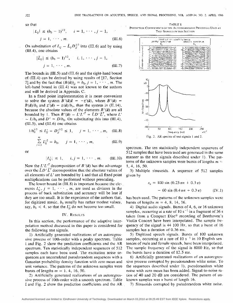
1) Artificially generated realizations of an autoregressive process of 10th-order with a peaky spectrum. Table I and Fig. 2 show the prediction coefficients and the AR spectrum. Ten statistically independent sequences of 512 samples each have been used. The excitation noise sequences are uncorrelated pseudorandom sequences with a Gaussian probability density function with zero mean and unit variance. The patterns of the unknown samples were bursts of lengths rn = 1, 4, 16, 50.

2) Artificially. generated realizations of an autoregressive process of 10th-order with a smooth spectrum. Table I and Fig. 2 show the prediction coefficients and the AR

TABLE I PREDICTION COEFFICIENTS OF THE AUTOREGRESSIVE PROCESSES USED A S

TEST SIGNALS I N THIS SECTIOV

dB

E -20- ...

-50 ~ - -60 0 50 100 150 200 250

Frequency IHzl .I02

Fig. 2. AR spectra of test signals I and 2.

spectrum. The ten statistically independent sequences of 5 12 samples that have been used are generated in the same manner as the test signals described under 1). The patterns of the unknown samples were bursts of lengths m = 1, 4, 16, 50.

3) Multiple sinusoids. A sequence of 512 samples given by

s, = 100 sin ( 0 . 2 3 ~ ~ + 0.3 T)

+ 60 sin ( 0 . 4 ~ ~ + 0 . 3 ~ ) (IV. 1)

has been used. The patterns of the unknown samples were bursts of lengths rn = 4, 8, 14, 16.

4) Digital audio signals. Bursts of 4, 6, or 16 unknown samples, occurring at a rate of 10 s- ' in a fragment of 36 s taken from a Compact Disc@ recording of Beethoven's Violin Concert have been interpolated. The sample frequency of the signal is 44 100 Hz, so that a burst of 16 samples has a duration of 0.36 ms.

5 ) Digitized speech signals. Bursts of 100 unknown samples, occurring at a rate of 10 s-' in 10 English sentences of male and female speech, have been interpolated. The sample frequency of the signal is 8000 Hz, so that the bursts have a duration of 12.5 ms.

6) Artificially generated realizations of an autoregressive process corrupted by pseudorandom white noise. To the sequences described under l ) , pseudorandom white noise with zero mean has been added. Signal-to-noise ratios of 40 and 20 dB are considered. The pattern of unknown samples was a burst of length 16.

7) Sinusoids corrupted by pseudorandom white noise.


JANSSEN et U L : ADAPTIVE INTERPOLATION OF DISCRETE-TIME SIGNALS 323

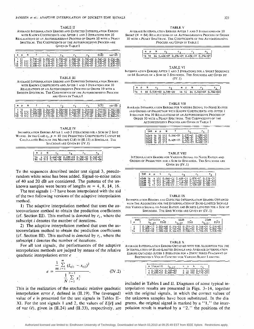
TABLE I1 AVERAGE INTERPOLATION ERRORS A N D EXPECTED INTERPOLATION ERRORS

WITH KNOWN COEFFICIENTS AND AFTER 1 AND 3 ITERATIONS FOR 10 REALIZATIONS OF AN AUTOREGRESSIVE PROCESS OF ORDER 10 WITH A PEAKY

SPECTRUM. THE COEFFICIENTS OF THE AUTOREGRESSIVE PROCESS ARE GIVEN IN TABLE 1

m p N f

4 10 512 0:lZE-Ol 0:llE-01 0:13E-01 0:13E-01 0:12E-01~0:61E-02 0:lOE-03 1 10 0 79E-02 0 90E-02 0 72E-02 0 90E-02 0 79E-02 0 34E-02 0 23E-04

16 10 512 0.26E-01 0.27E-01 O.26E-01 0.28E-01 0.26E-01 0.12E-01 0.67E-03 50 10 512 0.60E-01 0.61E-01 0.56E-01 0.62E-01 0.57E-01 0.24E-01 0.60E-02

_______-_____---____-- 41 _______ c3 --..---_ '1 _______ '3 ________-_____-______ E t a 1 var(J)

4 10 512 0.50Et00 0.62EtOO 0.62Et00 0.62Et00 0.61Et00 0.51Et00 0.76Et00 1 10 0.31Et00 0.34E+OO 0.32Et00 0.34Et00 0.32EtOO 0.27~+00 0.15~+00

50 10 512 0.11Et01 O.lIE+Ol O.llEt01 0.11Et01 0.11Et01 0.95E+00 0.39Et01 16 10 512 0.99Et00 O.lOE+OI 0.10Et00 O.lOEtO1 0.10Et01 0.84Et00 0.29Et01

TABLE IV INTERPOLATION ERRORS AFTER 1 AND 3 ITERATIONS FOR A SUM OF 2 SINE

WAVES. IN THE CASE Cj, p = 10 THE PREDICTION COEFFICIENTS CANNOT BE CALCULATED BECAUSE THE MATRIX c( i ) IN (11.13) IS SINGULAR. THE

SINUSOIDS ARE GIVEN BY (IV. I )

.............................................

To the sequences described under test signal 3, pseudorandom white noise has been added. Signal-to-noise ratios of 40 and 20 dB are considered. The patterns of the unknown samples were bursts of lengths rn = 4, 8, 14-, 16.

The test signals 1-7 have been interpolated with the aid of the two following versions of the adaptive interpolation method.

1) The adaptive interpolation method that uses the autocovariance method to obtain the prediction coefficients (cf. Section 111). This method is denoted by ci , where the subscript i denotes the number of iterations.

2) The adaptive interpolation method that uses the autocorrelation method to obtain the prediction coefficients (cf. Section 111). This method is denoted by ri , where the subscript i denotes the number of iterations.

For all test signals, the performances of the adaptive interpolation methods are judged by means of the relative quadratic interpolation error e ,

(IV .2)

This is the realization of the stochastic relative quadratic interpolation error 2, defined in (11.19). The (averaged) value of e is presented for the test signals in Tables II- XI. For the test signals 1 and 2, the values of E[&] and of var ( E ) , given in (11.24) and (11.33), respectively, are

TABLE V AVERAGE INTERPOLATION ERRORS AFTER 1 AND 3 ITERATIONS FOR 10

SHORT ( N = 64) REALIZATIONS OF AN AUTOREGRESSIVE PROCESS OF ORDER 10 WITH A PEAKY SPECTRUM. THE COEFFICIENTS OF THE AUTOREGRESSIVE

PROCESS A R E GIVEN I N TABLE 1

TABLE VI INTERPOLATION ERRORS AFTER 1 AND 3 ITERATIONS FOR A SHORT SEQUENCE

OF 64 SAMPLES OF A SUM OF 2 SINUSOIDS. THE SINUSOIDS ARE GIVEN BY (IV. 1)

TABLE VI1 AVERAGE INTERPOLATION ERRORS FOR VARIOUS SIGNAL-TO-NOISE RATIOS

AND ORDERS OF PREDICTION WITH KNOWN COEFFICIENTS AND AFTER 1 ITERATION FOR 10 REALIZATIONS OF AN AUTOREGRESSIVE PROCESS OF

ORDER 10 WITH A PEAKY SPECTRUM. THE COEFFICIENTS OF THE AUTOREGRESSIVE PROCESS ARE GIVEN IN TABLE I

TABLE VI11 INTERPOLATION ERRORS FOR VARIOUS SIGNAL-TO-NOISE RATIOS AND

ORDERS OF PREDICTION FOR A SUM OF SINUSOIDS. THE SINUSOIDS ARE GIVEN BY (Iv. 1)

4 0 d 6 ~ i 6 4-512 0.84E-02 0.40E-03 0.87E-01 0.21E-Dl 40dB 16 10 512 0 12E-03 0 11E-03 0 12E-03 0 12E-03 2Od8 16 4 512 0:38E+00 0:33E+00 0:44E+00 0:40EtOO 20d8 16 10 512 0.10E-01 0.11E-01 0.10E-01 0.10E-01

0.53E-13 0.00E+00 0.32E-01 0.25E-01 0.14E+01 0.25E+Ol 0.85E-06 D.OOE+OO 0.16Et02 0.84E+02 0.21E+04 0.84E+04 0.86E-02 0.00Et00 0.36E+03 0.50Et04 0.15Et05 0.50E+06

TABLE X

INTERPOLATION OF BAND-LIMITED SIGNALS A N D AVERAGE INTERPOLATION AVERAGE INTERPOLATION ERRORS OBTAINED WITH THE ALGORITHM FOR THE

ERRORS OBTAINED AFTER 1 ITERATION FOR A PREFILTERED FRAGMENT OF BEETHOVEN'S VIOLIN CONCERT FOR VARIOUS BURST LENGTHS

included in Tables I and 11. Diagrams of some typical interpolation results are presented in Figs. 3-14, together with the original signals, in which the correct values of the unknown samples have been substituted. In the diagrams, the original signal is marked by a " l , " the interpolation result is marked by a "2," the positions of the


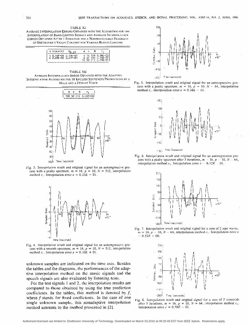
TABLE XI

INTERPOLATION OF BAND-LIMITED SIGNALS A N D AVERAGE INTERPOLATION AVERAGE INTERPOLATION ERRORS OBTAINED WITH THE ALGORITHM FOR THE

ERRORS OBTAINED AFTER 1 ITERATION FOR A NONPREFILTERED FRAGMENT OF BEETHOVEN'S VIOLIN CONCERT FOR VARIOUS BURSTS LENGTHS

____________________--------------------- 1 m t r a c e ( H ) b, _._. m D N r . I

TABLE XI1 AVERAGE INTERPOLATION ERROR OBTAINED WITH THE ADAPTIVE

INTERPOLATION ALGORITHM FOR 10 ENGLISH SENTENCES PRONOUNCED BY A MALE A N D A FEMALE VOICE

100r

80

60-

-

2 20-

- LO

0

U 0-

z 20-

40-

60L

80 -

1 5 ~ 1

100

50 0 0 - 0 0 V

a -

v)

5 -50

-100

-,5oL Tlme isecondsl

Fig. 5 . Interpolation result and original signal for an autoregressive process with a peaky spectrum, m = 16, p = 10, N = 64, interpolation method e , . Interpolation error e = 0.38E - 01.

1

1001 Time lsecondsl

Fig. 3. Interpolation result and original signal for an autoregressive process with a peaky spectrum, m = 16, p = 10, N = 512, interpolation method e, . Interpolation error e = 0.23E - 01.

Time (seconds)

Fig. 4. Interpolation result and original signal for an autoregressive process with a smooth spectrum, m = 16, p = IO, N = 512, interpolation method e, . Interpolation error e = 0. IOE + 01.

unknown samples are indicated on the time axis. Besides the tables and the diagrams, the performances of the adaptive interpolation method on the music signals and the speech signals are also evaluated by listening tests.

For the test signals 1 and 2, the interpolation results are compared to those obtained by using the true prediction coefficients. In the tables, this method is denoted by f , where f stands for fixed coefficients. In the case of one single unknown sample, this nonadaptive interpolation method amounts to the method presented in [2].

L

i .150L Tlme [seconds)

Fig. 6. Interpolation result and original signal for an autoregressive process with a peaky spectrum after 3 iterations, m = 16, p = 10, N = 64, interpolation method c3. Interpolation error e = 0.12E - 01.

2o01 150

-2001 Tlme isecondsl

Fig. 7. Interpolation result and original signal for a sum of 2 Sine waves, = 16, p = 10, N = 64, interpolation method e , . Interpolation error e

= 0.52E + 00.

200 I w l 100 1

-50 v) !!! -1 00 5 t

-1 50

- 2 O O L Tlme isecondsl

Fig. 8. Interpolation result and original signal for a sum of 2 sinusoids after 3 iterations, m = 16, p = I O , N = 64, interpolation method ci. Interpolation error e = 0.58E - 02.


JANSSEN ef al.: ADAPTIVE INTERPOLATION OF DISCRETE-TIME SIGNALS 325

.2001 Time isecondsi

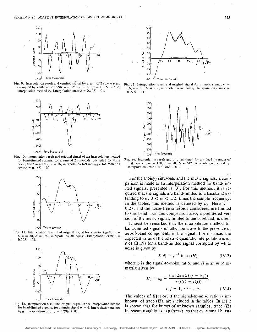
Fig. 9. Interpolation result and original signal for a sum of 2 sine waves, corrupted by white noise, SNR = 20 dB, m = 16, p = 10, N = 512, interpolation method c,. Interpolation error e = 0.10E - 01.

200,

-6ooL Time ( s e c o n d s )

Fig. 10. Interpolation result and original signal of the interpolation method for band-limited signals, for a sum of 2 sinusoids, corrupted by white noise, SNR = 40 dB, m = 16, interpolation method Interpolation error e = 0.16E + 02.

150r

2 0 I 8

5 V

E -50-

v?

-1 00 -

-150- Tlme Iseconds)

Fig. 11. Interpolation result and original signal for a music signal, m = 6, p = 20, N = 192, interpolation method r , . Interpolation error e = 0.59E - 02.

f

u v 2

-150L Time (seconds]

Fig. 12. Interpolation result and original signal of the interpolation method for band-limited signals, for a music signal m = 6, interpolation method bo,27. Interpolation error e = 0.28E + 01.

120 -

100-

80 -

60

LO

- -

0 + g 20-

- x 0- a

- 2 0 -

-LO

-00-

- -60

- w I \

/ Time (seconds)

Fig. 13. Interpolation result and original signal for a music signal, m = 16, p = 50, N = 512, interpolation method r , . Interpolation error e = 0.22E - 01.

1000-

800.

600 - Loa

-

2 200-

0- 0

Q g-200-

$400 - E

-600-

-800 -

. l o o ~ l Time (seconds1 '

Fig. 14. Interpolation result and original signal for a voiced fragment of mate speech, rn = 100, p = 50, N = 512, interpolation method r , . Interpolation error e = 0.70E - 01.

For the (noisy) sinusoids and the music signals, a comparison is made to an interpolation method for band-limited signals, presented is [ 3 ] . For this method, it is re- quired that the signals are band-limited to a baseband ex- tending to CY, 0 < a < 1/2, times the sample frequency. In the tables, this method is denoted by 6,. Here CY = 0.27, and the noise-free sinusoids considered are limited to this band. For this comparison also, a prefiltered version of the music signal, limited to the baseband, is used.

It must be remarked that the interpolation method for band-limited signals is rather sensitive to the presence of out-of-band components in the signal. For instance, the expected value of the relative quadratic interpolation error e" of (11.19) for a band-limited signal corrupted by white noise is given by

E [ ~ I = p - ' trace ( H ) (IV. 3)

where p is the signal-to-noise ratio, and H is an m X m- matrix given by

H . . = 6.. - 'J rJ

sin ( 2 ~ a ( t ( i ) - tu)) n(t( i ) - W ) '

i , j 1, * , m. (IV .4) The values of E[2] or, if the signal-to-noise ratio is unknown, of trace ( H ) , are included in the tables. In [ 3 ] it .is shown that for bursts of unknown samples, trace ( H ) increases roughly as exp ( T ~ c Y ) , so that even small bursts


326 IEEE TRANSACTIONS ON ACOUSTICS, SPEECH, AND SIGNAL PROCESSING, VOL. ASSP-34, KO. 2 , APRIL 1986

in signals with fairly high signal-to-noise ratios cannot be interpolated successfully.

The tables and figures show interpolation errors for various segment lengths and prediction orders. The true prediction orders of the artificially generated autoregressive processes and of the multiple sinusoids are known in ad- vance. For the autoregressive processes, the prediction order is 10; for the multiple sinusoids, the prediction order is twice the number of sinusoids in the signal, in this case p = 4. For these signals, the true prediction order is used in most cases, a higher prediction order is sometimes tried to achieve improvement in the interpolation quality. For the music and the speech signal, p = min (3m + 2, 50) is chosen. This rather arbitrary choice gives good interpolation results. The pattern of the unknown samples is always a burst. It has turned out that, as a rule, general patterns of unknown samples are usually interpolated with

, a smaller interpolation error than bursts with the same number of unknown samples.

The tables and figures give rise to the following re- marks. From Tables I1 and 111, it is seen that the interpolation errors for either adaptive method do not differ significantly from the interpolation errors for the interpolation method that uses the true prediction coefficients. It seems that the estimation of the prediction coefficients from the incomplete data does not influence the quality of the interpolation. The deviation of the average interpolation errors from the expected interpolation errors in Ta- bles I1 and I11 is explained by the high variance of the interpolation error. It is also seen from the Tables I1 and I11 that iterative use of the adaptive interpolation methods does not give a significant improvement. However, if the segment length N is smaller, iteration does give an improvement, as can be seen from Tables V and VI. Here results close to that of Tables I1 and I11 are obtained after 3 iterations. In general, the interpolation errors for autoregressive processes with a peaky spectrum are substan- tially smaller than for processes with a smooth spectrum.

For sinusoids 0 2 = 0, so that, theoretically, the interpolation error is also zero. Indeed, Table IV shows very small interpolation errors for methods cI and c3. The poorer results for r l , r3, p = 4 can be explained by the fact that the autocorrelation method uses a biased estimate for the autocorrelation function. This has less influence on the result if p is chosen higher. If the autocovariance method is used to estimate the prediction coefficients, p must not be chosen too high. For after more than one iteration, the autocovariance matrix will become nearly singular and the prediction coefficients can no longer be calculated straightforwardly by solving the system (11.13). As can be seen from the Tables 11, 111, VII, and VI11 for signals other than multiple sinusoids, there are no significant differences between the interpolation results obtained by using the autocovariance or the autocorrelation method.

With a decreasing signal-to-noise ratio, the interpolation results of the adaptive interpolation methods deteri- orate slightly. However, they still do not differ significantly from the results that can be obtained if the true

prediction coefficients were used. This can be seen from Tables VI1 and VIII. The interpolation method for band- limited signals gives poor results for noisy sinusoids, as can be seen from Table IX, where the quadratic interpolation error becomes several times larger than the signal energy.

For the music signal, the relative quadratic interpolation errors for the adaptive interpolation methods are of the same orders of magnitude as those for the autoregressive processes with a peaky spectrum. The high value for the relative quadratic interpolation error for the speech signal in Table XI1 can be explained as follows. In pop- ular speech models [ 181, speech is assumed to consist of voiced parts, where the speech signal is highly periodic, and unvoiced parts, where the speech can be modeled as an autoregressive process of order approximately 12. In the voiced case, the speech spectrum contains many sharp equidistant peaks, and the interpolation results are similar to those obtained with autoregressive signals that have a peaky spectrum. In the unvoiced case, the speech spectrum is rather flat, and the interpolation results are similar to those obtained with autoregressive signals with a smooth spectrum. As can be seen from Table I11 and Fig. 4, these results are rather poor, especially if the bursts are large. The relative quadratic interpolation error in Table XI1 is averaged over 20 sentences and the high value is caused by the presence of unvoiced fragments. However, the poor interpolation results for unvoiced fragments do not cause any audible disturbance in the interpolated speech. Fig. 14 shows a typical interpolation result for voiced speech.

Listening tests have revealed that the interpolation errors in these test signals and in many other signals are practically inaudible. After increasing the burst length from 16 to 50, the interpolation results are still quite good for most music signals, although some interpolation errors become audible. For the speech signals, bursts can be restored up to 100 unknown samples without audible errors. It may seem curious that the method still works for bursts of these lengths (which represent time intervals of durations up to 12.5 ms), since the length N of the segment used to estimate the prediction coefficients repre- sents a time interval of more than 60 ms which is gener- ally too long for a speech signal to be assumed stationary. However, some speech sounds, for instance vowels, can be assumed stationary for several hundreds of milliseconds, and for these the method performs well. Other speech sounds, especially the plosive sounds, lbf, fdi, l g i , lpf, lti, and l k f , can only be assumed stationary for a few milliseconds and cannot be interpolated correctly. Still, the errors made here do not seem to reduce the sub- jective interpolation quality, possibly because of masking effects.

Comparing the adaptive interpolation method to the interpolation method for band-limited signals, it is seen that the latter method performs better if the burst length m is small, say, m I 6, and if no out-of-band components are present in the signal. If these requirements are not met, it .gives very poor results, as can be seen from Table XI


JANSSEN ef al.: ADAPTIVE INTERPOLATION OF DISCRETE-TIME SIGNALS 327

and Figs. 10 and 1 2 . Usually, the errors are pulse shaped and may well exceed the peak values of the signal. The adaptive interpolation method performs significantly better in the presence of noise or for large bursts.

V. CONCLUSIONS In this paper, an adaptive method has been presented

for the interpolation of general patterns of unknown samples occurring in discrete-time signals that can be modeled as autoregressive processes. It has been demon- strated that this method gives satisfactory 'results for digital audio signals and digitized speech. Roughly speak- ing, the method amounts to trying to minimize, as a function of the unknown samples and the unknown prediction coefficients, a sum- of squares of residual errors involving the unknown samples, the prediction coefficients, and the known samples from a sufficiently large neighborhood. The method can be used noniteratively as well as iteratively. In the noniterative case, one minimization step with respect to the prediction coefficients and, subsequently, one with respect to the unknown samples are performed. In the iterative case, the subsequent minimizations are performed repeatedly, the current estimates of the unknown samples being employed in each iteration step. It- eration gives an improvement in interpolation quality if a relatively small segment of data is available.

The interpolation method has been shown to have a sound mathematical foundation. Also, it can be related to several well-known estimation methods in statistics and linear filtering. Furthermore, when applied to signals sat- isfying the model assumption, the expected quadratic interpolation error per sample is bounded asymptotically by the signal energy.

The method has been tested on artificially generated autoregressive processes, sinusoids, digital audio signals, and digitized speech signals. The performance has been judged both objectively and subjectively. It has been observed that the interpolation method is capable of restoring satisfactorily at least 16 consecutive unknown samples in an audio signal sampled at 44 100 Hz, corresponding to a time interval of 0.36 ms, and in a speech signal, sampled at 8000 Hz up to 100 consecutive unknown samples, corresponding to a time interval of 12.5 ms.

It has been shown that the various minimizations can be carried out by efficiently solving, in a stable manner, certain systems of linear equations. This indicates that the interpolation method is suitable for a fixed point implementation in an integrated circuit. However, in that case, the number of unknown samples should not be too high (up to 16, say).

APPENDIX A ANALYSIS OF Q (a , x)

In this appendix, the claims of Section I1 are proved that, if the sample values have a Gaussian probability density function,

1) minimizing Q(a, x) for known x as a function of a leads to a maximum likelihood estimate for a , and

2) minimizing Q(a, x) for known a as a function of x leads to a minimum variance estimate for a.

Furthermore, it is shown that the integral in (11.6) attains its minimum as a function of x for the same value as Q(a, x) does.

A. Maximum Likelihood Estimation of a for Known x

ability density functions It is assumed that the Zk are independent and have prob-

The log likelihood function that is usually taken to get maximum likelihood estimates for a:, a from a sequence s = [so, - - * , s,,,-~]' of data is log (ps(slo:, a) ) , the logarithm of the probability density function of .F. The log likelihood function in (11.6) differs slightly from this. However, it can be shown that for large N (compared to p ) one may approximate the more commonly used one by the one in (11.6) [ 191.

To express L(a5, a) in terms of Q ( a , x), one observes that

p~ltdslu, a e , a) = PS; . , f ! t l - (sp, * * * > s N - , Iu, U e , a> 2 2

- - Pfp+ I , ' ' ' ,fN- IISO, ' ' ' , fp

X ( s p + l , * * 3 sN- 11~0, * * * 3 sp, a e , a)

( A . 2 )

2

x PfpTpl&pIu? a,, 4 . 2

Furthermore,

By repeatedly applying

2 ~ s l d s l u , a e , a)

0 4 . 3 ) the above reasoning,, one finds that

N - p

Therefore, L(O& a) = -(N - p ) log (a,&) - Q(u, x)/(2a;).

(A. 5 ) Maximizing L(a$, a) as a function of a is the same as minimizing &(a , x) as a function of a . This proves the claim. Furthermore, of can be estimated by maximizing L ( o ~ , a) as a function of a:. This gives the estimate in (11.5) if m = 0 is taken.

B. Minimum Variance Estimation of the Unknown Samples

It is shown that, under hypothesis (A . l ) , finding the minimum variance estimate for x, given a and sk, k = 0,


. . . , N - 1, k # t ( l ) , * , t (m) is the same as minimizing Q ( a , x) as a function of x. To this end, one can use the well-known fact from statistical estimation theory that the minimum variance estimator Go of a stochastic vector G, given a stochastic vector i7 equals E[@t(i7], the expectation under yndition i7. Hence, for the minimum variance estimator f0 o f f , given the known samples one has

io = E[x”lq”l (A. 6)

where the known samples are arranged in a vector i j . To evaluate this, one needs p f l q (x 14). It is straightforward to show that

Pf(q(x14) = Ps~i(sIu)/Pqli(41u). (A. 7)

By using (A.4), one can express the right-hand side of $4.7) in terms of Q (a , x). More specifically, one has for f0

where D is such that

D x exp ( -Q(a , x)/(2a:)) dx = 1. (A.9)

It follows from a standard fact about Gaussian integrals that Q(a , x), a quadratic form in x, is minimized by 6, in (A.8). This proves the claim.

Observe also that io maximizes p f l q ( x 14) as a function of x. This shows that is also a maximum a posteriori estimates for x. This follows further from (A.7) and (A.4).

A further result is that io = -(B(a))-I z(a) is also the best linear minimum variance estimator. This result holds without any assumptions on the form of the probability density function of the excitation noise. Indeed, it is a well-known fact that the best linear minimum variance estimator is completely determined by the covariances

hypothesis of Gaussian probability density functions, the minimum variance estimator io happens to depend lin- early on the known samples, as is seen from (11.14), (11.1 l ) , and (11.12). Thus, io is certainly the best linear minimum variance estimator, whether or not Gaussian probability density functions have been assumed.

r .m

E[g,gk], j , k = 0, * * , N - 1. Furthermore, under the

On inserting the definition (11.17) into (A. l l ) and per- forming the integration, one finds for the integral in (11.16)

. N-0-1 (A. 12)

for properly chosen constants a > 0, b E R?. This proves that the P of (11.14) minimizes the integral in (11.16) as a function of x”.

APPENDIX B SOME NOTES ON THE ITERATIVE VERSION OF THE

INTERPOLATION METHOD A. Convergence Properties

Iterating the interpolation method comes down to con- structing two sequences d ( k ) E RP and i ( k ) E R* of vec- tors of prediction coefficients and sample estimates, respectively. Here d (1) = B and i ( 1) = i , B and i as in (11.13) and (11.14). In the kth step, d ( k ) and i ( k ) are obtained by minimizing Q ( a , i ( k - 1)) with respect to a and Q ( B ( k ) , x) with respect to x, respectively. That is,

Q(d(k ) , i ( k - 1)) = min Q(a, P(k - 1)) (B.l) a € ’

It was found that iterating the interpolation method can improve the results if the number of available samples is relatively small. Although the iterative method turns out to converge very rapidly in practice (cf. Section IV for more details), it does not seem easy to prove satisfactory convergence results. It can be shown that, when the sequences d ( k ) , P ( k ) converge, the limit point a’, x ‘ is a stationary point. However, Q(a , x) may have several such points. For the .asymptotic speed of convergence, the Hessian H of Q(a, x) at a’ , x ’ is relevant. Letting

H ’ = ~ l:iJAA:l (B. 3)

whereA, = (a2/aa2)Q((a’,x’),A2 = ( a 2 / a a d x ) Q ( a ’ , x ‘ ) and A3 = (d2/ax2) Q(a’, x’ ) , one can check that

A, = 2C(xr) ,

A2 = 2(ei+t(j) + f - i + t ( j ) ) i = l ; . . , p , j = l : . . . r n ’

A3 = ~ B ( u ’ ) , (B.4) C. A Spectral Interpretation

its minimum for the same.x as Q(a , x) does. It is useful ek = C aisk-jn to note that

where, with = x : , i = 1, * * * 9 m, It is shown that for fixed a, the integral (11.16) attains P

l = O

P N - p - I

Q ( U , X) = C SkSlbk-l + E (A. 10) = C aiSk+i. 03.5) k;/ = p 1 = 0

Since where E involves only samples with indexes I , k < p or I , k > N - p - 1. The integral (11.16) can be written as

&(a, X) G Q ( a r , x r ) + 1/2(a - u ‘ ) ~ A ~ ( u - a ’ )

+ (a - a’ )TA2(x - x r )


JANSSEN et ul.: ADAPTIVE INTERPOLATION OF DISCRETE-TIME SIGNALS 329

it follows that

P(k + 1) z X ' + AT1A;A;'A2(P(k) - x' ) . (B.7)

The speed of convergence of the iterative method is determined by the spectral properties of D = A; 'A&4;IA2. A condition guaranteeing linear convergence is that the absolute values of the eigenvalues of DTD are all less than 1, but it does not seem easy to check on this condition.

B. Relation to the EM Algorithm The assumption is that the observed s = [so, * * * ,

sN- is a vector of realizations of a stationary Gaussian autoregressive process of known order p and unknown prediction coefficients u E R f and a:. Consider the log likelihood function

L(a2, a) = - ( N - p )

- log (a,&) - Q(a, x)l(20f). (B.9)

The EM algorithm aims at finding estimates for parameters and complete data from incomplete data by maximizing the (log) likelihood .function. It can be described for the present situation a's follows: Denote for (a:, a) E R X Rl P

W ( O $ ~ , a*lof, a) = E[L(az2, a*)lq, a:, a ] , (B.lO)

with q as in (A.6). Starting with initial estimates &f(O), ci(O), one constructs sequences &f(k), ci(k), k = 1 , 2 , * - . , by choosing in the kth step B:(k), b(k) in such a way that ~ ( a : , al$f(k - I ) , ci(k - 1)) is maximal at (a:, a) = (3f(k), ci(k)). Heuristically, one would like to maximize L (o:, a) , but this is impossible since one does not know s completely.

To show the connection with the iterative interpolation method, it is necessary to evaluate (B. 10). The conditional expectation in (B. 10) refers to the conditional probability density

(B. 11) It follows that

w e 2 , a*laf, a) = - ( N - p ) log (a,*&)

- E[Q(a*, x>lq, of , a I l ( 2 ~ $ ~ ) .

(B. 12)

It is a tedious but straightforward calculation to show that

E[C?(a", 4 I q , a:, a1

= u t trace ((B(a))-'B(a*)) + Q(a*, x), (B.13)

so that one has

W(aT2, a*lof, a) = - ( N - p ) log (a,*&)

- 1/2(0,/0,*)~ trace ( (B(U) ) - 'B(U*) )

- Q(u*, X). (B. 14)

Maximizing W ( a z 2 , a*Iuz, a) is the same as minimizing the right-hand side of (B.13). Hence, the difference between the EM algorithm and the iterative version of the adaptive interpolation method is reflected by the first term in the right:hand side of (B. 13). It is noted that minimizing Q(a*, x) with 'respect to a* is much easier than minimizing the right-hand side of (B. 13), since it is not likely that a manageable form for the solution of the latter problem exists.

APPENDIX C DECOMPOSITION OF B(a)

In this appendix, the left-hand inequality of (111.4) is proved. First, remark that

B(a) = ATA, (C. 1)

whereA = [ a l , * - , a,] is a ( t (m) - t(1) + p + 1) x m-matrix, defined by

the a i being the prediction coefficients of (11.1). Note that a i = 0 for i < 0 or i > p . Since A has full rank, A can be decomposed as a product A = QR, where Q is a ( t (m) - t (1) + p + 1) X m-matrix, consisting of m orthogonal columns and R is an upper triangular m X m-matrix. On substituting A = QR into (C. l ) , one obtains

B(a) = RTQTQR = LDLT (C. 3)

where L" and D are as in (111.3). Clearly, Djj = lqj 1 2 . The QR decomposition of A can be done iteratively. In every iteration step, qj is found by subtracting from a j the pro- jection of aj onto the space spanned by q l , * * * 4j-I

The space sp{ql, * , q j p 1 } spanned by q l , - qj- 1 is the same as the space sp{al, * , aj - ] spanned by al, * * uj'- Therefore,

- - min (a j - U I 2 u€Sp{uI. ' ' ' , u j - I }

i - 1

Since ( a j ) r ( j ) - t ( t ) + p + l = ao = 1 and ( a k ) t ( J ) - t ( l ) + p + l = Ofork = 1, - * , j , by (C.2), it follows easily that ( q j I * 2 1. This proves the left-hand inequality of (111.4).

ACKNOWLEDGMENT The authors wish to thank their colleague H. J. Prins for

his help in finding a convenient approach to the solution of the interpolation problem, and for drawing their attention to the EM algorithm.


330 IEEE TRANSACTIONS ON ACOUSTICS, SPEECH, AND SIGNAL PROCESSING, VOL. ASSP-34, NO. 2 , APRIL 1986

REFERENCES [ l ] R. Steele and F. Benjamin, “Sample reduction and subsequent adap-

tive interpolation of speech signals,” Bell. Syst. Tech. J . , vol. 62, no. 6, pp. 1365-1398, 1983.

121 S. M. Kay, “Some results in linear interpolation theory,” IEEE Trans. Acoust., Speech, Signal Processing, vol. ASSP-31, pp. 746-749, June 1983.

[3] A. J. E. M Janssen and L. B. Vries, “Interpolation of band-limited discrete-time signals by minimizing out-of-band energy,” in Proc. ICASSP ’84, San Diego, CA, 1984.

[4] H. Akaike, “A new look at the statistical model identification,” IEEE Trans. Automat. Cuntr., vol. AC-19, pp. 716-728, June 1974.

151 S. M. Kay and S. L. Marple, Jr . , “Spectrum analysis-A modern perspective,” Proc. IEEE, vol. 69, no. 11, pp. 1380-1419, 1981.

[6] A. P. Dempster, N. M. Laird, and D. B. Rubin, “Maximum likelihood from incomplete data via the EM algorithm,” J . Roy. Stat. Soc., Series B , vol. 39, pp. 1-38, 1977.

[7] C. F. J. Wu, “On the convergence properties of the EM algorithm,” Ann. Stat., vol. 11, no. 1, pp. 95-103, 1983.

[SI R. A. Bayles, “On the convergence of the EM algorithm,” J . Roy. Stat. SOC. , Series B , vol. 45, no. 1, pp. 47-50, 1983.

[9] F. Itakura and S. Saito, “A statistical method for estimation of speech spectral density and formant frequencies,” Electron. Commun. Ja- pan, vol. 53-A, pp. 36-43, 1970.

[lo] I . I. Hirschmann, Jr., “Recent developments in the theory of finite Toeplitz operators,” in Advances in Probability and Related Topics, vol. 1. New York: Marcel Dekker, 1971.

[ 11 j M. Marcus and H. Minc, Introduction to Linear Algebra. New York: MacMillan, 1965.

1121 J. Durbin, “The fitting of time-series models,” Rev. Inst. Int. Stat., vol. 28, pp. 233-243, 1960.

[13] G . Cybenko, “The numerical stability of the Levinson-Durbin algorithm for Toeplitz systems of equations,” SIAM J . Sci. Stat. Com-

[14] J. H. Wilkinson, The Algebraic Eigenvalue Problem. Oxford, En- gland: Clarendon 1965.

1151 N. Levinson, “The Wiener rms (root mean square) error criterion in filter design and prediction,” J . Math Phys., vol. 25, pp. 261-278, 1947.

1161 P. Delsarte, Y . Genin, and Y. Kamp, “A polynomial approach to the generalized Levinson algorithm, based on the Toeplitz distance,” IEEE Trans. Inform. Theory, vol. IT-29, pp. 268-278, 1983.

[17] J. H. Wilkinson, “Error analysis of direct methods of matrix inver- sion,” J . Assoc. Compur. Mach., vol. 8, pp. 281-330, 1961.

[18] L. R. Rabiner and R. W. Schafer, Digital Processing of Speech Sig- nals. Englewood Cliffs, NJ: Prentice-Hall, 1978.

[19] S. M. Kay, “Recursive maximum likelihood estimation of autoregressive processes,” IEEE Trans. Acoust., Speech, Signal Process- ing, vol. ASSP-31, pp. 56-65, Feb. 1983.

put., V O ~ . 1, pp. 303-320, 1980.

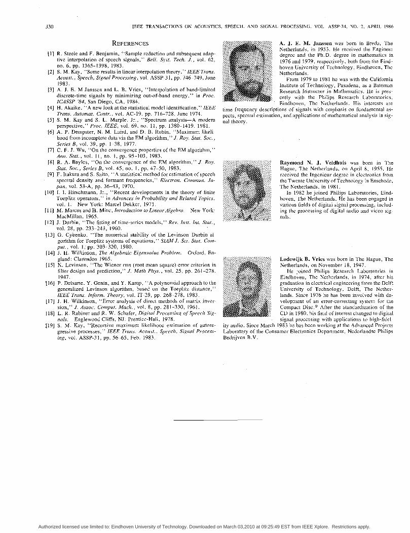
Raymond N. J. Veldhuis was born in The Hague, The Netherlands, on April 8, 1955. He received the Ingenieur degree in electronics from the Twente University of Technology in Enschede, The Netherlands, in 1981.

In 1982 he joined Philips Laboratories, Eind- hoven, The Netherlands. He has been engaged in various fields of digital signal processing, includ- ing the processing of digital audio and video signals.


jkIalexandria.tue.nl/openaccess/Metis235417.pdfjkI I (b) Fig. 1. (a) Sequence containing a burst of...

Documents

Transcript of jkIalexandria.tue.nl/openaccess/Metis235417.pdfjkI I (b) Fig. 1. (a) Sequence containing a burst of...