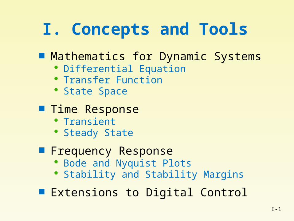
I-1

I. Concepts and Tools Mathematics for Dynamic Systems

Differential Equation Transfer Function State Space

Time Response Transient Steady State

Frequency Response Bode and Nyquist Plots Stability and Stability Margins

Extensions to Digital Control

I-2

A Differential Equation of Motion

Newton’s Law:

A Linear Approximation:

( ) ( , ( ), ( ), ( )) ( )y t f t y t y t w t bu t

( ) ( ) ( ) ( )TKy t y t w t u tJ J

I-3

Laplace Transform and Transfer Function

2

( ) ( ) ( )

( ) ( ) ( ) ( )

( )( )

( ) ( )

T

T

Tp

Ky t y t u t

J J

Ks Y s sY s U s

J J

Y s KG s

U s s Js

0( ) ( ) stY s y t e dt

I-4

State Space Description

1 2

1 1

2 2

1

2

( ) ( ) ( )

,

0 1 0

0

[1 0]

T

T

Ky t y t u t

J J

x y x y

x xuK

x xJ J

xy

x

1

2

0 1 0,

0

[1 0], D=0

T

xLet x

x

x Ax Bu

y Cx Du

with

A B K

J JC

I-5

From State Space to Transfer Function

1( ) ( )

=( )

p

T

G s C sI A B D

K

s Js

I-6

Linear System Concepts

States form a linear vector space Controllable Subspace and Controllability Observable Subspace and Observability The Linear Time Invariance (LTI) Assumptions Stability

Lyapunov Stability (for linear or nonlinear systems) LTI System Stability: poles/eigenvalues in RHP

I-7

A Motion ControlProblem

LOAD

DRIVE

PULLEYASSEMBLY

J L

J D

N L

N D

N PD

N PL

WL0

r

r WL

M WL

r WDO

WDr

M WD

TD

J P

L

D

LT

B L L

DDB

B TRL

L

LLT J TR

L

LTRLJ

EQUIVALENTMODEL

I-8

L T TT J B

L D TT T gr

L T

D T T

grTF

T s J s B

D CS S A TT v K K K

( ) L S A T T

pCS T T

K K K grG s

v s J s B

From Differential Eq. To Transfer Function

I-9

( ) S A T T

pT T

K K K grG s

s J s B

Transfer Function model of the motion plant

( )p

KG s

s Js

I-10

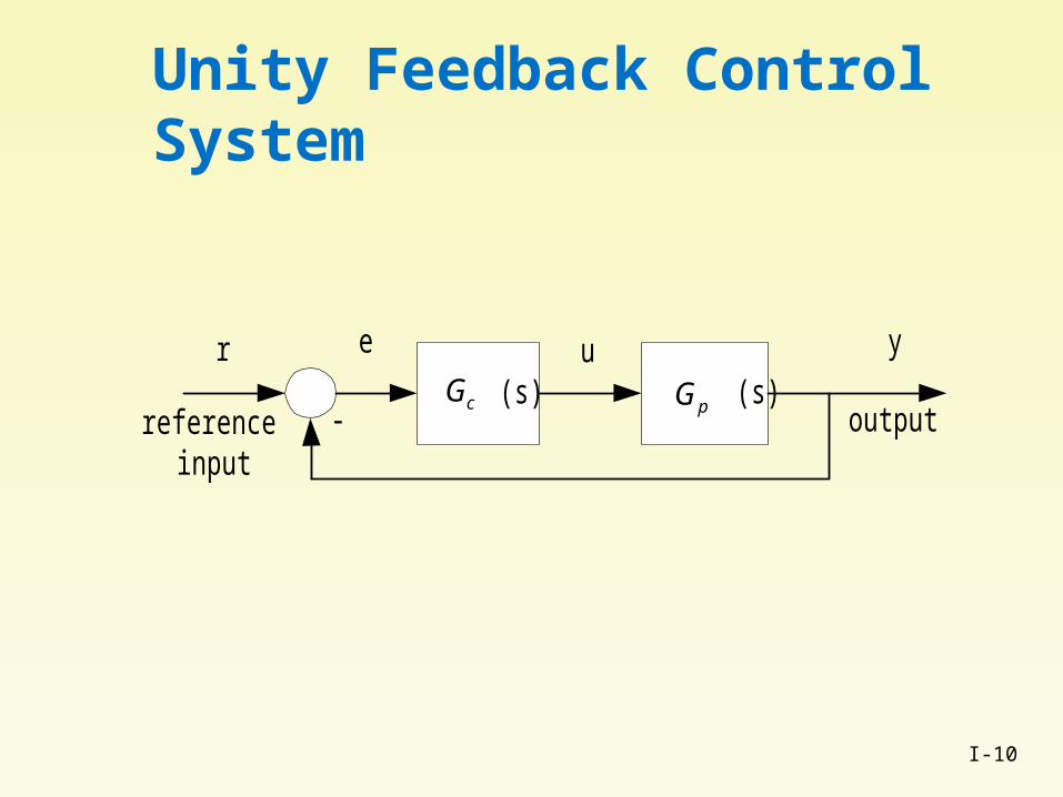
Unity Feedback Control System

(s)-

(s)r ye

referenceinput

outputpGcGu

I-11

Common Nonlinearities

I-12

Linearization

I-13

Time Response

I-14

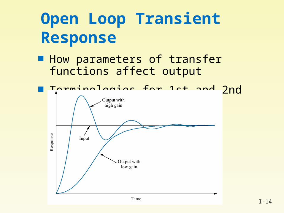
Open Loop Transient Response

How parameters of transfer functions affect output Terminologies for 1st and 2nd order systems

I-15

Basis of Analysis

I-16

First Order Transfer Function

( )

1

1

aG s

s a

s

I-17

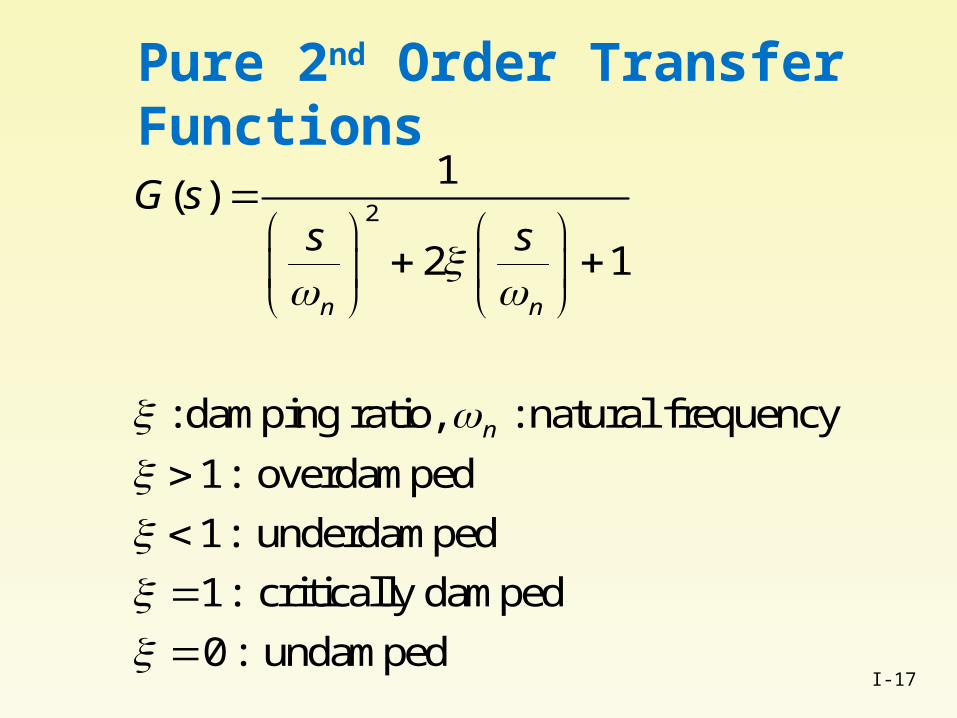
Pure 2nd Order Transfer Functions

2

1( )

2 1

: damping ratio, : natural frequency

1: overdamped

1: underdamped

1: critically damped

0 : undamped

n n

n

G ss s

I-18

Pure 2nd Order Transfer Functions

I-19

Pure 2nd Order Transfer Functions

I-20

Terminologies

max% 100final

final

c cOS

c

I-21

Calculations

2( / 1 )% 100

4s

n

OS e

T

I-22

Pure 2nd Order Transfer Functions

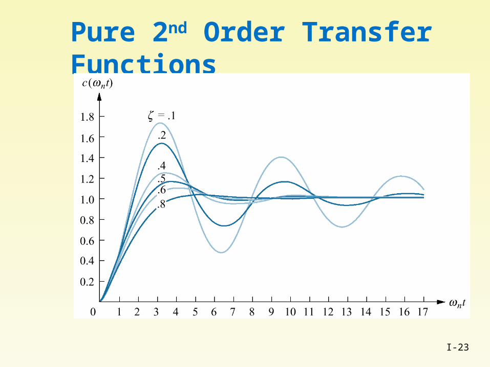
I-23

Pure 2nd Order Transfer Functions

I-24

Pure 2nd Order Transfer Functions

I-25

Steady State Response

Steady state response is determined by the dc gain: G(0)

I-26

Steady State Error

(s)-

(s)r ye

referenceinput

outputpGcGu

0( ) | ( ) |

( )( )

1 ( ) ( )

ss t s

c p

e e t sE s

R sE s

G s G s

I-27

Frequency Response: The MOST useful concept in control theory

Performance Measures Bandwidth Disturbance Rejection Noise Sensitivity

Stability Yes or No? Stability Margins (closeness to instability) Robustness (generalized stability margins)

I-28

Frequency Response

I-29

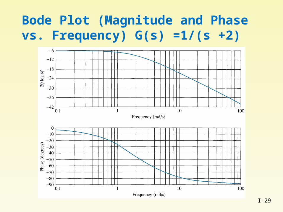
Bode Plot (Magnitude and Phase vs. Frequency) G(s) =1/(s +2)

I-30

Polar Plot: imaginary part vs. real part of G(j) G(s) =1/(s +2)

I-31

Bandwidth of Feedback Control

-3dB Frequency of CLTF

0 dB Crossing Frequency (c) of Gc(j)Gp(j)

Defines how fast y follows r

(s)-

(s)r ye

referenceinput

outputpGcGu

( ) ( )( )

( ) 1 ( ) ( )c p

c p

G j G jY j

R j G j G j

I-32

Disturbance Rejection

(s)-

(s)0 y

outputpGcG

d

( ) 1

( ) 1 ( ) ( )

measures disturbance rejection quality

c p

Y j

D j G j G j

I-33

Noise Sensitivity

(s)-

(s)0 y

pGcG

n

u

noise

( ) ( )

( ) 1 ( ) ( )

( ) at high frequency

c

c p

c

U j G j

N j G j G j

G j

I-34

Nyquist Plot

Using G (j) to determine the stability of

-

r y( )G s

( )H s

( ) ( ) ( )

( ) : Sensor and Filter

c pG s G s G s

H s

I-35

The Idea of Mapping

I-36

Nyquist Contour

j

j

s j RHP

I-37

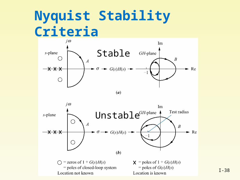
Nyquist Stability Criteria

Determine stability by inspection Assume G(s)H(s) is stable, let s complete the N-

countourThe closed-loop system is stable if G(s)H(s)

does not encircle the (-1,0) point Basis of Stability Robustness Further Reading: unstable G(s)H(s), # of unstable

poles

I-38

Nyquist Stability Criteria

Stable

Unstable

I-39

Stability Robustness

The (-1,0) point on the GH-plane becomes the focus Distance to instability:

G(s)H(s)-(-1)=1+G(s)H(s) Robust Stability Condition

Distance to instability > Dynamic Variations of G(s)H(s)

This is basis of modern robust control theory

I-40

Gain and Phase Margins(-1,0) is equivalent of 0dbpoint on Bode plot

G(j)H(j)

G(j)H(j)|

I-41

Stability Margins:

Bode PlotNyquist Plot

I-42

Digital Control

I-43

Discrete Signals

I-44

Digital Control Concepts

Sampling Rate Delay

ADC and DAC Resolution (quantization levels) Speed Aliasing

Digital Control AlgorithmDifference equation

I-45

Discrete System Description

Discrete system

h[n]: impulse response

Difference equation

h[n]u[n] y[n]

0 0

[ ] [ ]N M

k kk k

a y n k b u n k

I-46

Discrete Fourier Transform and z-Transform

X(e j ) x[n]e j

n

X(z) x[n]z n

n

I-47

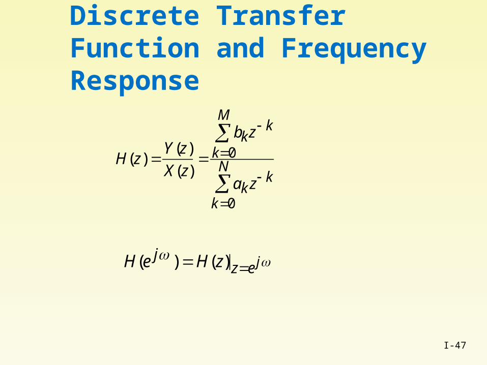
Discrete Transfer Function and Frequency Response

H(e j ) H(z) ze j

H(z) Y(z)

X(z)

bkz k

k0

M

ak z k

k0

N

I-48

Application of Basic Concepts to Previously Designed Controllers