Hysteresis, Price Acceptance, and Reference Prices

Timothy J. Richards, Arizona State University, trichards@asu.eduMiguel I. Gómez, Cornell University, mig7@cornell.edu

Iryna Printezis, Arizona State University, iiermole@asu.edu�

Selected Paper prepared for presentation at theAgricultural and Applied Economics Association�s 2014 Annual Meeting,

Minneapolis, MN, July 27-29, 2014.

March 18, 2014

�Copyright 2014 by Timothy J. Richards, Miguel I. Gomez, and Iryna Printezis. All rights reserved. Readers may makeverbatim copies of this document for non-commercial purposes by any means, provided that this copyright notice appears onall such copies.

1 Introduction

Shelf prices are not always the stimulus consumers use to guide their decision making. Rather, the existence

of reference prices, or mental benchmarks consumers use to assess what is a "normal" or expected price,

is well-documented (Lattin and Bucklin 1989; Hardie, Johnson, and Fader 1993; Kalyanaram and Winer

1995; Bell and Lattin 2000; Erdem, Mayhew, and Sun 2001; Mazumdar, Raj, and Sinha 2005; Pauwels,

Srinivasan, and Franses 2007). From a practical standpoint, however, practitioners are more interested in

what happens when prices move away from the reference level? Empirical studies reveal zones of inactivity

around reference prices, or "latitudes of price acceptance" (Gupta and Cooper 1992; Kalwani and Yim 1992;

Kalyanaram and Little 1994; Han, Gupta, and Lehmann 2001; Terui and Dahana 2006) in which retail prices

change, but consumers do not appear to respond as we would expect them to. That is, consumers appear to

be insensitive to price changes between an upper and lower threshold surrounding the reference price. One

popular explanation for the existence of such price-thresholds is the Assimilation-Contrast Theory (ACT,

Sherif 1963) in which �a new stimulus encountered by an individual is judged against a background of previous

experience in the category�(Kalyanaram and Little 1994). Price variations within the region of acceptance

are assimilated, or ignored, and price changes outside of this region are contrasted with the consumer�s

previous experience, thereby inducing a behavioral response. Others explain the fundamental asymmetry

in consumer response around their reference price in terms of either Prospect Theory (PT, Kahneman and

Tversky 1979) or Adaptation Level Theory (ALT, Helson 1964). Prospect Theory maintains that consumers

develop an expected or reference price, and that any price changes above that level will leave them in the

domain of losses, while price reductions below their reference level will leave them in the domain of gains.

Because losses are perceived as more onerous than gains are bene�cial, according to Prospect Theory, loss

aversion leads to a revealed asymmetry in price response that appears as a kinked demand curve. Adaptation

Level Theory, on the other hand, argues that consumers will not respond to a stimulus if it is not deemed to

be either too high or too low relative to some benchmark price that they have become adapted to. However,

each of these theories presumes some sort of behavioral component that contradicts the underlying tenets of

rational economic behavior. While such violations are possible, and well-documented, the burden of proof

in documenting their existence is high because they remove the ability of theory to generalize and to explain

1

market phenomenon that result from individual behavior.1 In this study, we o¤er an alternative that is

grounded in rational economic behavior.

Our explanation, on the other hand, does not require that we assume the market fails when thresholds

arise. Rather, if consumers face uncertain retail prices, and incur �xed costs in searching for grocery products

(Mehta, Rajiv, and Srinivasan 2003; Hong and Shum 2006; Moraga-Gonzalez and Wildenbeest 2008; Kim,

Albuquerque, and Bronnenberg 2010; Wildenbeest 2011; De los Santos, Hortacsu, and Wildenbeest 2012),

then the purchase decision embodies a real option value. Akin to a �nancial option to buy a share of stock

(or currency, commodity contract, or other �nancial instrument) at a �xed price for a �xed time period, the

ability to wait until the uncertainty surrounding the retail price is resolved creates a potentially signi�cant

value for the option holder. Consequently, the decision to purchase the product when shelf prices are either

above or below the reference price involves exercising the option and giving up a substantial amount of value

in doing so. Allowing the shelf price to change either upward or downward su¢ cient to make exercising this

option worthwhile creates a zone of apparent acceptance around the reference price in which the consumer

neither capitalizes on the opportunity to take advantage of a perceived "deal" on the product, nor reluctantly

responds to an underlying need for a product that is deemed relatively expensive. Intuitively, consumers

know that if retail prices are volatile, there is a chance that the price will fall far enough to make immediate

purchase a wise decision, and that there is also a chance that the price will rise far enough to cause them to

have to ful�ll a need at an apparently usurious price. Waiting for either to happen creates inactivity that is

referred to as hysteresis (Dixit and Pyndick 1994), or the persistence of a phenomenon even after its initial

cause has disappeared. Identifying hysteresis, as opposed to either ACT, PT, or ALT, requires that we

estimate a threshold econometric model in which the location of the thresholds depends on factors that drive

real option values, namely past price volatility. None of the alternative explanations for the existence of

price thresholds depends on the volatility of retail prices in this sense, so if retail price volatility is found to

be a signi�cant determinant of the price thresholds, then the data support our hysteretic theory of threshold

formation.2

1For example, if everyone in the market possesses a di¤erent reference price, then there is no reason to explain why thresholdsarise in aggregate data, despite evidence that they do (Pauwels, Srinivasan, and Franses 2007) and empirical evidence thatheterogeneity explains much of the evidence of reference prices, traditionally de�ned (Lattin and Bucklin 1989).

2Others conjecture that the size of the zone of price acceptance depends, in part, on price volatility (Mazumdar and Jun1992), but do not formalize why this might be the case.

2

We test our hysteretic explanation for the presence of a latitude of price acceptance using household-

level scanner data from four frequently-purchased product categories (that vary in their purchase frequency;

cereal, yogurt, and laundry soap) in a variant of an econometric friction model (Rosett 1959). A friction

model is appropriate for testing the theory that underlies threshold pricing because it explicitly accounts for

the existence of thresholds in the data that separate households into regimes of gains, losses, and indi¤erence

based on some endogenous source of censoring. In our model, the selection mechanism derives from price

volatility and a real option e¤ect. Terui and Dehana (2006) is the only other study that explicitly accounts for

the data-censoring implied by threshold behavior, but their model presumes a Bayesian separation mechanism

and normally distributed preferences. We allow for randomness in the formation of price thresholds as in Han,

Gupta and Lehmann (2001), but the latter do not account for the underlying censoring of the data caused by

thresholds. While their model is an extension of a logit model of brand choice, ours represents a fundamentally

di¤erent approach to accounting for threshold-price behavior. Accounting for unobserved heterogeneity in

the hysteretic e¤ect addresses the issue of whether price acceptance is an artefact of heterogeneity in our

data (Bell and Lattin 2000), or are inherently probabilistic constructs (Han, Gupta, and Lehmann 2001). If

removing unobserved heterogeneity causes thresholds to disappear, then it is clear that thresholds are due

to failing to account for unobserved factors that otherwise explain reference-price e¤ects.

We compare our model to other possible explanations � ACT, PT, ALT � in order to establish the

validity of our model. The primary di¤erentiating factor between the hysteretic and other models is that the

threshold driven by an implicit real option will widen when the variability of prices is high. That is, when a

retail price is relatively volatile, the real option will be higher, so the hysteretic e¤ect will be stronger, and

the threshold wider than would otherwise be the case. The other explanations for reference-price behavior

are silent on the e¤ect of two-sided volatility on the existence and magnitude of price-thresholds. We compare

these models using commonly-accepted models that embed reference prices, and use the speci�cation for the

formation of reference prices that has been found to �t the data from several categories best (Briesch et al.

1997). Consequently, observations of market-level threshold e¤ects must be explained by something other

than micro-level household behavior.

Our �ndings have practical importance. Marketing practitioners use the concept of �threshold e¤ects�as

3

if it was of the order of a stylized fact (Management Science Associates 2013). That is, the implicit assumption

among practitioners is that demand response is not smooth over a range of prices, but rather there exists

pricing thresholds beyond which demand elasticities change in a fundamental way. Whether this is true or

not is critically important for setting retail prices, because elasticities clearly drive the relationship between

pricing and sales revenue. In order to be useful, a method of estimating demand models that accounts for,

and is able to test for and locate, such thresholds, must be relatively simple and tractable in a relatively large

demand system. In this research, we develop an approach for estimating pricing thresholds and demonstrate

its usefulness in four frequently purchased consumer good categories. Many studies identify the existence

of reservation prices and thresholds at the micro, household-level (Mazumdar, Raj, and Sinha 2005). While

individual behavior may be the source of any reservation price behavior, marketers are more interested

in the aggregate, market-level implications of individual-level reservation prices. Pauwels, Srinivasan and

Franses (2007) address this problem by estimating a reservation-price model in aggregate data, but with a

demand model that is not grounded in utility maximization. Bell and Lattin (2000) show that much of the

reservation price evidence disappears once heterogeneity is properly accounted for, but not all. The question

remains, therefore, are threshold-prices a product of aggregate, store-level data? Rather than estimate with

store-level data, we estimate our threshold-price model at the individual household level, and then simulate

a market equilibrium over an assumed distribution for unobserved consumer heterogeneity. Any thresholds

that remain, therefore, are both consistent with individual utility maximization, and the distribution of

heterogeneity that is relevant for practitioners.

We �nd that the data are consistent with our hysteretic explanation for threshold prices. One of the

primary implications of the hysteretic model that di¤erentiates it from others is that the size of the latitude

of price acceptance rises in the volatility of retail prices. Because option values rise in volatility, the implicit

cost of excercising the option by making a purchase is higher the more variable retail prices. We �nd strong

evidence in support of this outcome in each of the product categories. Second, we �nd evidence of asymmetric

price response above and below the threshold. This �nding suggests that, while Prospect Theory may not

provide a complete explanation of threshold-price behavior, its predictions are nonetheless relevant in data.

Third, we �nd that consumers do appear to respond to variations in retail prices around reference levels, even

4

after controlling for heterogeneity in both the threshold and in price response. This �nding is signi�cant as

reference-price formation does not appear to be an artefact of failing to control for unobserved heterogeneity.

Finally, we �nd that our household-level estimates do indeed imply aggregate, or store-level, threshold price

behavior. Because store-level data remains the workhorse of marketing analytics in practice, our �ndings

are relevant to decision-makers.

Our �ndings contribute to both the theoretical and methodological literatures on reference prices and

price thresholds. Conceptually, �nding support for our hysteretic model of threshold price e¤ects adds

an explanation for an oft-observed phenomenon that does not rely on some sort of a behavioral deviation

from neo-classical economic assumptions. Although it is not our intent to discredit behavioral models in

general, nor to justify traditional economic modeling, our model shows how predictions based on simple

postulates of consumer behavior are su¢ ciently general and should not be ruled out. Our approach also

adds to the existing literature on this topic by synthesizing theory from �nancial economics with marketing

theory to arrive at an alternative explanation for what is generally regarded as a stylized fact. On a

methodological level, we contribute to the debate on whether the existence of reference prices and price

thresholds are artifacts of failing to control for unobserved heterogeneity. In our model, we allow for two

sources of consumer heterogeneity and still �nd evidence of reference-price behavior. We also explicitly

account for the implications of threshold-price behavior for censoring e¤ects in the underlying data, and o¤er

a tractable, easily-estimated alternative to existing Bayesian methods of estimating multi-threshold demand

models. Finally, we contribute to the body of empirical evidence on the asymmetry of price-response to

either side of price thresholds. Speci�cally, Prospect Theory suggests that consumers respond much more

aggressively to price increases than to price reductions, and we �nd evidence to support this hypothesis in

frequently-purchased consumer-packaged goods data.

In the second section, we provide a brief background to the theoretical and empirical literature on reference

prices and price thresholds. We use this background to motivate the development of an alternative model in

section three that is based in real option pricing theory, and its primary implication for purchase behavior,

purchase hysteresis. We present our econometric model of purchase hysteresis in the fourth section, and

describe how we implement the model in data covering four categories of consumer packaged goods. The

5

application and relevant data are presented in a �fth section. We o¤er detailed estimation results from one

category in the sixth section, and compare our �ndings to alternative model speci�cations. We also discuss

our results in the context of other empirical research on this issue. A �nal section concludes, and suggests

some avenues for future research that may help resolve some of the fundamental debates that remain.

2 Background on Reference Prices and Price Thresholds

In this section, we summarize the theories used to explain the existence of reference prices, and how they

may give rise to thresholds in consumer decision making. These theories are grouped into three broad

classi�cations as to their origin: (1) neo-classical economics, (2) consumer behavior and applied psychology,

and (3) �nancial economics. We summarize the �rst two in this section, and o¤er our alternative as part

of the third group of explanations in the next section. There we describe how our new theory of threshold

prices compares with existing theories in terms of its implications for observed pricing patterns, and retail

practice.

2.1 Neo-Classical Economic Theories

While demand curves in principles of economics are typically represented as smooth and continuous, the

notion of a "kinked" demand curve arose early in the theory of imperfect competition with di¤erentiated

products. Sweezy (1939) was the �rst to advance the notion that rival �rms in oligopoly will match price

increases, but not price reductions. Therefore, if an individual �rm tries to raise its price, it loses a large

amount of market share, but cannot gain much market share by reducing its price. In the kinked-demand

story, however, it is di¢ cult to disentangle whether the observed response in demand derives from consumer

behavior, or a rational �rm response to expectations of consumer behavior.3 Similarly, more recent research

on the apparent �xity of retail prices cites the existence of �xed costs (termed "menu costs") of changing

prices as an explanation for apparent thresholds in price response. Such �xed costs introduce a fundamental

non-convexity to �rms�price-change decision so that prices will not change smoothly in response to under-

lying changes in demand or costs, but rather follow an (sL; S; sU ) bounds rule (Sheshinski and Weiss 1977;

Caballero and Engel 1999; Slade 1998, 1999). According to this rule, a retailer may want to change her price

3Subsequent empirical research by Stigler (1947) and Simon (1969) discredited the kinked-demand curve theory by �ndingthat oligopoly �rms do not necessarily respond in the most dis-advantageous way to the initiator of a price change.

6

toward an �ideal�level, S, but she will only do so when the bene�t of a change exceeds the total adjustment

cost. Once the desired price reaches either an upper or lower threshold, it is immediately changed to the

target value. Putler (1992) also demonstrates the implications of reference-price behavior for neo-classical

market equilibrium, but does not attempt to explain why reference prices arise in the �rst place.

2.2 Behavioral Theories

Several theories in consumer behavior and applied psychology have been developed to explain reference prices

and their link to the existence of thresholds in consumer decision making. The �rst was Adaptation Level

Theory (ALT), put forward in pioneering research by Helson (1964). In the context of reference prices, ALT

posits that a consumer�s price reference point is determined by her exposure and recollection of prior prices.

Monroe (1971) and Della, Bitta and Monroe (1974) empirically test this theory in experimental settings

to show that consumers respond di¤erently when prices are above the reference price than when they are

below the reference price. Subsequent research based in ALT focused on implications to price advertising

(Gotlieb and Dubinsky 1991), pricing of new products (Della, Bitta and Monroe 1974), the role of retail

prices suggested by suppliers (Lichtenstein and Bearden 1988), and pricing tactics (Kinard, Capella and

Bonner 2013), among others. While this stream of research points out to the importance of the level of

retail price relative to the reference price of consumers, it is silent regarding how large the di¤erence between

reference and actual prices should be to trigger changes in purchase decisions.

Various theories have been developed to examine the nuances of identifying reference price structure,

relying on quantitative methods for testing (Winer 1986). By far, the most popular among these are Assimi-

lation Contrast Theory (ACT, Sherif and Hovland 1961; Sherif 1963) and Prospect Theory (PT, Kahneman

and Tversky 1979). The two theories di¤er in their assumptions about the in�uence of the reference price,

in particular regarding the existence of discontinuities in the relationship among reference prices, actual

prices and consumer response (Boztug and Hildebrand 2005). Most research has focused on PT, although

a large body of consumer behavior literature suggests that reference price may be a region and should not

be described as a point (Emery 1969; Kalwani and Yim 1992; Klein and Oglethorpe 1987; Monroe 1971;

Sawyer and Dickson 1984). Moreover, a growing number of empirical studies con�rm the existence of price

thresholds (Han, Gupta, and Lehmann 2001; Kalyanaram and Little 1994; Raman and Bass 2002; Pauwels,

7

Franses, and Srinivasan 2004).

Assimilation Contrast Theory (ACT) was introduced Sherif and Hovland (1961) based on the psycho-

logical principle that individuals have a range of indi¤erence around a reference point. According to ACT,

a stimulus inside this indi¤erence range is perceived as smaller than its real value (i.e., assimilation e¤ect).

On the other hand, stimulus outside the range of indi¤erence is perceived as larger than its real value (i.e.,

contrast e¤ect) triggering behavioral changes of individuals. Sherif (1963) was the �rst in applying ACT to

consumer price perception and in measuring the range of indi¤erence in an experimental setting. Lichten-

stein and Bearden (1989) examine the range of acceptance around the expected market price. The authors

assume an asymmetric range of indi¤erence around the reference price. Kalyanaram and Little (1994), in-

tegrate ACT with a consumer choice model assuming a symmetric range of indi¤erence to gaps between

actual prices and the reference price. They also included price variability when determining the width of the

indi¤erence range. The primary challenge of using ACT to build a consumer choice model is to determine the

width of the range of indi¤erence, which has to be estimated from experiments or from consumer purchase

data.

Contrary to ACT, Prospect Theory (PT, Kahneman and Tversky 1979) generally assumes a range of

zero around the reference price and the indi¤erence region thus becomes a point (Boztug and Hildebrand

2005). A fundamental characteristic of PT is that individuals tend to value losses more than gains (i.e. when

prices are lower and higher than the reference price, respectively). The theory assumes that consumer utility

is concave for gains and convex for losses; and that individuals are loss-averse with the loss function being

steeper than the gains function (Edwards, 1996; Tversky and Kahneman 1981). PT has been often employed

to describe pricing decisions under risk (Levy and Wiener 2013; Urbany and Dickson 1990; Edwards 1996).

Most empirical applications of PT have focused on �nancial markets, particularly on the price of �nancial

assets and the evaluation of investment alternatives (e.g., Loughran and McDonald 2013; Henderson 2012;

Gurevich, Kliger and Levy 2009). However, empirical applications o¤er a number of managerial and market-

ing implications. For example, Kalyanaram and Winer (1995) and Choi et al. (2013) employ PT to show that

the timing and magnitude of price promotions should take into account the existence of reference prices and

their resulting demand impacts. Janiszewski and Lichtenstein (1999) demonstrate that the range of evoked

8

prices moderates the e¤ect of reference price and has implications for �high-low�and �every-day-low price�

pricing strategies. Moreover, researchers have shown that reference prices, together with the way they are

shaped, in�uence brand choices and purchase quantity decisions (Kumar, Kirande and Reinartz 1998). PT

has also been used to show that macroeconomic factors such as interest rates, unemployment and in�ation

in�uence the formation of reference prices and should therefore be taken into account in the evaluation of

alternative pricing strategies (Estelami, Lehmann and Holden 2001).

Neither neo-classical nor behavioral theories of threshold pricing are entirely satisfactory. While neo-

classical models o¤er a rigorous explanation for how thresholds can arise from rational, optimizing behavior,

they are silent on how the value of the thresholds is determined. On the other hand, behavioral theories

implicitly assume a failure on the part of consumers to rationally consider all available information, or to

respond in less-than-rational ways to price changes. In the next section, we o¤er an alternative to both that

is grounded in optimizing behavior, and provides estimates of threshold values that are empirically tractable.

3 Conceptual Model of Purchase Hysteresis

The theory of purchase hysteresis derives from the concept of a real option from the �nancial economics

literature (Dixit 1989; 1992). In this section, we demonstrate how a real option arises in a household�s pur-

chase decision, and how this gives rise to a hysteretic e¤ect. This hysteretic e¤ect, in turn, is observationally

equivalent to the latitude of price acceptance observed by other authors.

In an uncertain retail-price environment, the �xed costs of searching for and purchasing a good embed

a real option in the purchase decision. The value of this real option rises in the level of price volatility,

which provides a convenient way to test for the existence of a real option. Before testing econometrically

for the presence of a real option e¤ect, we argue why, logically, shopping for and purchasing consumer goods

must include a real option component. Speci�cally, there are three necessary conditions that must exist for

a real option value to arise: (1) ongoing uncertainty, (2) �xed costs, and (3) a unique opportunity to make

a decision (Dixit 1989). The long-term volatility of retail prices is not controversial. Whether from retail

promotions, retailers passing through trade promotions, cost increases, or meeting competitive challenges,

there are many factors that may cause retail prices to vary over time. Second, Mehta, Rajiv, and Srinivasan

9

(2003) document the magnitude of search costs in a retail grocery environment. Third, individual consumers

clearly have sovereignty over their purchase decisions, so there is no market mechanism through which the

real option value will be arbitraged away. In summary, the appropriate conditions exist for a purchase

decision to embody a real option value, one that is signi�cant relative to the shelf price of the product. In

this section, therefore, we develop a simple mathematical model of how real options can be expected to arise

in grocery purchases, and derive an econometric model that can test for their presence in household-level

scanner data.

Solving for the dynamically optimal purchase process under price uncertainty results in a discontinuous

purchase path similar to one that would arise with a model of economic friction (Rosett 1959). If the

cost of purchasing a consumer product in a retail store includes a real-option component, then we expect

to see a consumer respond to prices that rise above his or her reference price only if a certain threshold

"price gap" (di¤erence between the shelf price and reference price) has been reached, and respond to a price

reduction only if the price gap falls below a di¤erent threshold value. When retail purchases are subject

to price thresholds, consumers are in the domain of gains when the shelf price falls below the reference

price (Kahneman and Tversky 1979), or in the domain of losses when self prices rise above their reference

price. Because the size of the threshold includes both a generalized measure of search costs and a real option

value, the consumer follows a discontinuous purchase strategy wherein the gap between the upper and lower

purchase-price thresholds widens with the value of the option. We show how this result occurs by deriving

a consumer�s reference price and then demonstrating how it is likely to di¤er from the observed stimulus

price, or the price that leads to either purchasing or switching.

To make our concept of the source of volatility concrete, consider a retail food product such as co¤ee or

cereal, where the production cost is largely driven the price of the underlying commodity, and production

labor. While labor is relatively stable, and predictable, the commodity cost can lead to wide variation in the

costs of production. Witness the general price of groceries during the 2008 commodity boom, the 2009 bust,

and the subsequent resurgence of commodity prices. Wholesale prices over this period were particularly

volatile, and recent research on retail pass-through rates (Eichenbaum et al 2011; Gopinath et al 2011)

suggest the same was true at retail. De�ne the gap between a consumer�s reference price and the observed

10

shelf price as follows: ghjt = rphjt � pjt for consumer h, brand j, and period t: Reference prices are assumed

to be brand-speci�c given the empirical evidence on the preferred speci�cation for reference-prices (Briesch

et al. 1997). Note that this de�nition is not standard, but we feel it is more intuitive as the consumer gains

if shelf prices fall below the reference price (or the value of ghjt rises). If retail prices are indeed uncertain,

then they are expected to follow a stochastic process over time. For simplicity, we assume the relationship

between a consumer�s reference price and the retail price follows a Geometric Brownian Motion process:

dghj = �jghj dt+ �jg

hj dz; (1)

suppressing the time subscript, where � is the mean drift rate, � is the standard deviation of the process, and

dz de�nes the Wiener increment with properties: E(dz) = 0; E(dz2) = dt: Search costs consist of opportunity

costs of the consumer�s time, travel costs, or even cognitive processing costs that are incurred in �nding a

product, considering alternatives, and making a purchase (Roberts and Lattin 1991), each of which is sunk,

or irretrievable after the search process has been completed. De�ne these costs generically as cht as they vary

across consumers, and over time.

From a consumer�s perspective, his or her wealth is conceptualized as the present value of a stream of

lifetime consumption decisions, plus the value of other investments. If the consumer�s objective is to maxi-

mize the wealth, or the value, of his or her household by making optimal purchase decisions, the fundamental

arbitrage condition that determines the value of the real option compares the value of a household that pur-

chases (V p;h) with one that does not purchase (V n;h): Faced with a decision of purchasing or not purchasing

at each period, the maximum value a household can attain is the maximum of whether it purchases or does

not purchase, or:

V 0;h(ghj ; pjt; t) = max[Vn;h(ghj ; pjt); V

p;h(pjt)� �cht ]; (2)

where � is the marginal cost of search, assuming search takes place only when a purchase occurs.4 The

solution to this problem provides upper and lower threshold values of ghjt that constitute optimal switching

points between responding and not responding to a particular value of the price gap.

4A shopping trip is de�ned as a purchase occasion in which the household is observed making at least one purchase, notnecessarily in the focal category.

11

Unlike other price-threshold models, ours maintains that in order for a consumer to purchase a brand,

the di¤erence between the shelf and reference prices must be large enough to not only cover the direct costs

of search, but also the implicit option value of waiting to make a purchase. Exercising this option (and

thus purchasing or switching) means sacri�cing an asset of real value to the household, therefore, doing so

represents a real and signi�cant opportunity cost. Indeed, even for small search costs, ongoing uncertainty

in the price gap can cause a wide gap between the latent desire to purchase and observed purchase behavior.

Given the stochastic process governing price gaps, there may be a long wait for the shelf price to either rise

or fall enough to induce a stimulus for purchase behavior, where "wait" is de�ned in terms of a range of

retail prices between the upper and lower response thresholds. This wait is interpreted as the latitude of

price acceptance (Kalyanaram and Little 1994), or hysteresis in purchase behavior.

The problem described in (2) above can be solved using dynamic programming techniques (Caballero and

Engel 1999; Slade 1999), but a contingent claims approach (Dixit 1989, 1992) provides analytical expressions

for the threshold values of ghj that are amenable to econometric estimation. Contingent claims analysis treats

the value of waiting to make a purchase as a contingent security �contingent on the underlying price-process

upon which the decision depends. Compare the value of a household that decides to purchase with one that

does not using the value functions in (2). With search costs, and uncertainty of the form shown in (1), the

value of a household that does not purchase consists of one capitalized stream of purchase decisions, plus

the value of the option to purchase, while the value of a household that does purchase is the discounted

value of a consumption stream that includes the most current decision. Given the process for ghjt shown

in (1), the equilibrium condition for a household that decides not to purchase is found by �rst equating

the instantaneous expected return on household wealth due to a change in the price gap with the required

return on the household�s wealth (�V n). In this case, the instantaneous expected return consists only of the

expected rise in the value of the household (Dixit 1989) so the partial di¤erential equation becomes:5

(1=2)�2g2V ngg + �gVng � �V n = 0; (3)

where we note that subscripts indicate partial di¤erentiation, we suppress the household indices for clarity,

5The rise in the net worth of the household is akin to holding equity in a publicly-traded �rm only for its expected capitalgain.

12

� is the required rate of return, and the other variables are as previously de�ned. The general solution to

(3) is then found by substituting g� = V n and solving the resulting quadratic equation:

�(�) = (1=2)�2�(� � 1) + �� � � = 0; (4)

where � is a constant to be determined. This equation has two roots: �1 < 0, and �2 > 1 such that:

�1; �2 = 1=2

0@1� 2��2

+ =� �

1� 2��2

�2+8�

�2

!1=21A : (5)

the general solution to the di¤erential equation (3) for a household that does not purchase must re�ect this

fact so we write:

V n = Ang�1 +Bng�2 ; (6)

which must then be solved for values of An and Bn. The fact that this expression solves (3) can be veri�ed

by taking the �rst and second derivatives of V n in (6) and substituting the result into (3). As in Dixit (1989),

the two terms on the right-side of (6) represent the option to purchase, while the value of not purchasing is

normalized to zero by assumption.

We determine the value of the option by applying the value-matching and smooth pasting conditions to

the expressions for the value of a non-purchasing household, and one that responds to the price-gap stimulus.

The value of a household that decides to purchase is determined solely by the �ow of services provided by

the good as they have already exercised the option to buy. The value of the good, in turn, is assumed to

be equal to the price gap as it represents the di¤erence between what a household is willing to pay for the

good, and what the market requires them to pay. Because the price gap is assumed to drift at an average

rate of �; the present value of this stream of bene�ts to the household is found as:

V a =g

�� �; (7)

for a constant �, so the value of the household is comprised entirely of the value of purchasing the good

in question. Solving for the constant terms is possible if we recognize that for small values of g the value

13

of the option to wait will be very low, so An = 0. Further, at a su¢ ciently high level of g, call it the

upper-threshold, or gU , a household will immediately purchase so the value of a non-purchasing household

must equal the value of a household that does purchase less the �xed cost of search:

V n(gU ) = Bn(gU )�2 =gU + p� rp

�� � � �c = V a(gU ); (8)

because the value of a household that purchases is equal to the capitalized value of all desired consumption.

Next, the smooth pasting condition requires that the incremental value of waiting to purchase as g rises

must be equal to the incremental value of a household that has already purchased, or:

V ng (gU ) = �2Bn(gU )�2�1 = 1=(�� �) = V ag (g

U ): (9)

The smooth pasting and value matching conditions yield two equations and two unknowns. Solving these

for gU gives a closed-form expression for the threshold price gap as a function of the parameters of the model:

gU =

��2

�2 � 1

�(�c(�� �)� �=�) ; (10)

where �2 is a function of both the drift rate and volatility of the price gap, and is strictly greater than one

in value.

Using traditional economic decision rules, a household in this environment purchases if the gains are

greater than the annualized �xed cost of shopping and buying: gU > �c(� � �): However, because �2 is

greater than one, the existence of a real option creates a wedge between the traditional and "full cost"

thresholds that depends on the volatility of underlying prices and the magnitude of search costs (Dixit

1992; Dixit and Pindyck 1994). A similar line of reasoning applies in calculating the value of gL. If retail

prices are falling, consumers will wait until the observed price falls below not only the reference price, but

also the cost of shopping and the a real option of not purchasing. As a result, the lower threshold price

gap is signi�cantly below zero. Combining both upper and lower thresholds, observed price gaps imply a

discontinuous pattern of purchasing with no activity over a wide range of observed shelf prices. De�ning the

indirect utility associated with a price gap of gt as U(gt), a consumer�s purchase behavior maximizes the

indirect utility function given by:

14

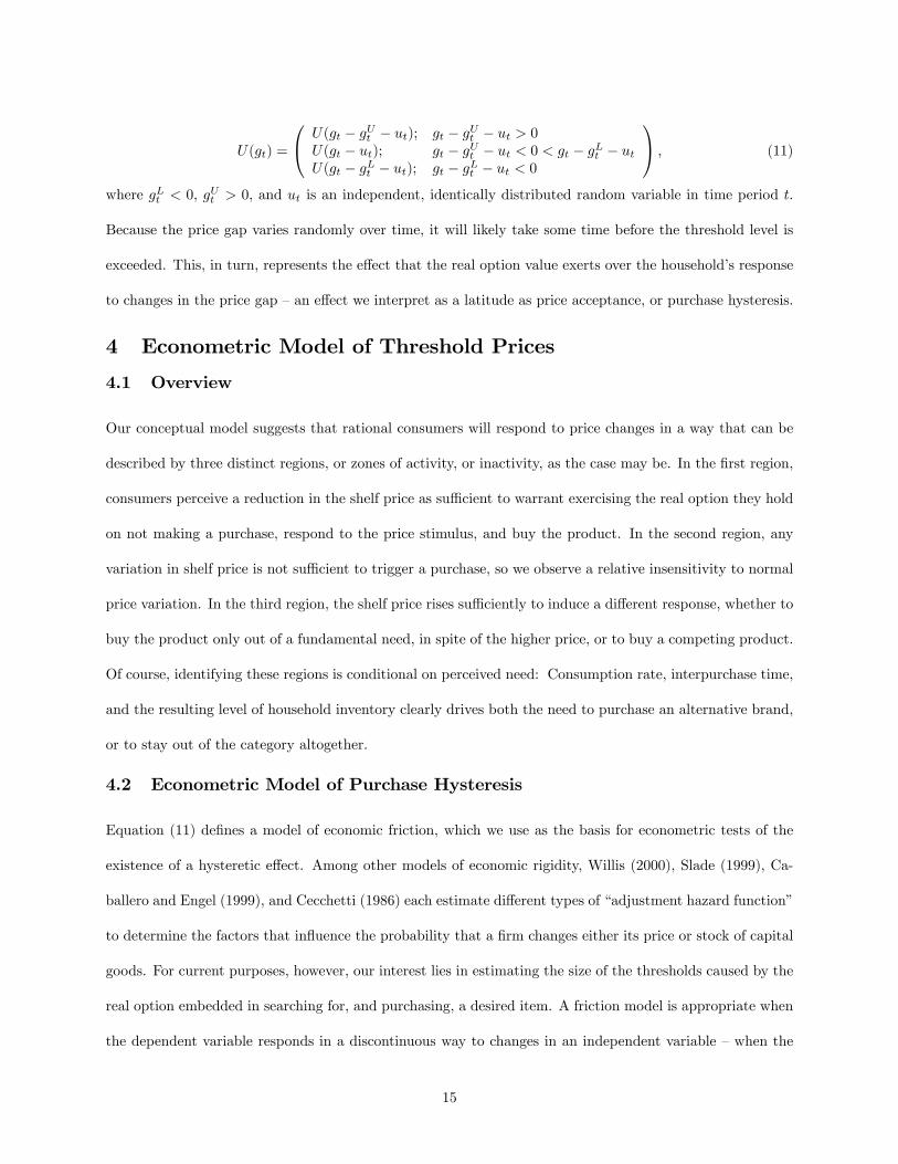
U(gt) =

0@ U(gt � gUt � ut); gt � gUt � ut > 0U(gt � ut); gt � gUt � ut < 0 < gt � gLt � utU(gt � gLt � ut); gt � gLt � ut < 0

1A ; (11)

where gLt < 0; gUt > 0, and ut is an independent, identically distributed random variable in time period t.

Because the price gap varies randomly over time, it will likely take some time before the threshold level is

exceeded. This, in turn, represents the e¤ect that the real option value exerts over the household�s response

to changes in the price gap �an e¤ect we interpret as a latitude as price acceptance, or purchase hysteresis.

4 Econometric Model of Threshold Prices

4.1 Overview

Our conceptual model suggests that rational consumers will respond to price changes in a way that can be

described by three distinct regions, or zones of activity, or inactivity, as the case may be. In the �rst region,

consumers perceive a reduction in the shelf price as su¢ cient to warrant exercising the real option they hold

on not making a purchase, respond to the price stimulus, and buy the product. In the second region, any

variation in shelf price is not su¢ cient to trigger a purchase, so we observe a relative insensitivity to normal

price variation. In the third region, the shelf price rises su¢ ciently to induce a di¤erent response, whether to

buy the product only out of a fundamental need, in spite of the higher price, or to buy a competing product.

Of course, identifying these regions is conditional on perceived need: Consumption rate, interpurchase time,

and the resulting level of household inventory clearly drives both the need to purchase an alternative brand,

or to stay out of the category altogether.

4.2 Econometric Model of Purchase Hysteresis

Equation (11) de�nes a model of economic friction, which we use as the basis for econometric tests of the

existence of a hysteretic e¤ect. Among other models of economic rigidity, Willis (2000), Slade (1999), Ca-

ballero and Engel (1999), and Cecchetti (1986) each estimate di¤erent types of �adjustment hazard function�

to determine the factors that in�uence the probability that a �rm changes either its price or stock of capital

goods. For current purposes, however, our interest lies in estimating the size of the thresholds caused by the

real option embedded in searching for, and purchasing, a desired item. A friction model is appropriate when

the dependent variable responds in a discontinuous way to changes in an independent variable �when the

15

latent stimulus for activity must exceed a certain threshold level before a response is observed (Rosett 1959;

Maddala 1983). In Rosett�s (1959) example, he models the response of asset holdings to changes in their

yield. Due to unobservable transactions costs, only relatively large changes in yield cause a reallocation.

With this approach, we are able to estimate the size of each threshold as well as test the e¤ect of each

explanatory variable on the real option value that is likely present.

There are a number of econometric implications of the real option e¤ect that are manifest in the friction

model. First, we will not observe a consumer response to a price gap despite considerable variation in a

latent (unobservable utility) desire to do so. Second, the extent to which latent utility �uctuates before a

response occurs, or the threshold price gap, will rise with its expected volatility. Third, the gap between the

upper and lower thresholds will widen with the magnitude of search costs. Fourth, purchases will exhibit

signi�cant inertia, meaning that when purchases do occur, the underlying decision will not change even after

their apparent cause has disappeared, and �fth, upward price changes need bear no quantitative relationship

to the size of downward price changes so response will appear to be asymmetric (Kahneman and Tversky

1979). Each of these hypotheses is tested within an estimable form of (11) wherein we do not observe

purchases or switches until the di¤erence between reference and shelf prices either rises above, or falls below

a certain threshold level. To arrive at this form of the model, however, we �rst de�ne each of the theoretical

constructs that are thought to underlie purchase hysteresis.

Utility is a function of not only the price gap, but elements of the marketing mix, brand-speci�c prefer-

ence, brand loyalty, and category inventory. We de�ne household-speci�c reference prices as a brand-level,

geometric weighted average of past prices. In doing so, we follow Briesch et al. (1997) who test a number of

speci�cations for the reference price, and �nd that a household-speci�c, geometric weighted average provided

the best �t. The friction model suggests that there is no reason why price response should be symmetric

on either side of the full-cost thresholds, so we let the parameters of interest vary across regimes of rising,

falling, and staying the same.

In order to test the purchase hysteresis model outlined above, we disaggregate the price gap into observable

and unobservable components, and the observable part into regimes in which the reference price is above the

current shelf price, below the shelf price, and equal to the shelf price. De�ne this part of the price gap as

16

lying in the domain of gains (G) when the shelf price is below the household-speci�c reference price (gh;Gjt ),

in the domain of losses (S) when the shelf price is above the reference price (gh;Sjt ), or neither (A) when the

observed price is equal to the reference price. The unobservable component, however, it what separates our

model from others in the price-acceptance literature. Namely, we de�ne the upper and lower threshold price

gaps to be parametric functions of the underlying volatility of prices: gUjt = U�g and gLjt = L�g. Although

Han, Gupta, and Lehmann (2001) allow their probabilistic thresholds to depend on price volatility, their

motivation is empirical, and not grounded in a model of option pricing as is ours. With this speci�cation, if

U 6= 0 and L 6= 0, then our data support the theory of purchase hysteresis when controlling for all other

possible explanations for the existence of a zone of price acceptance.

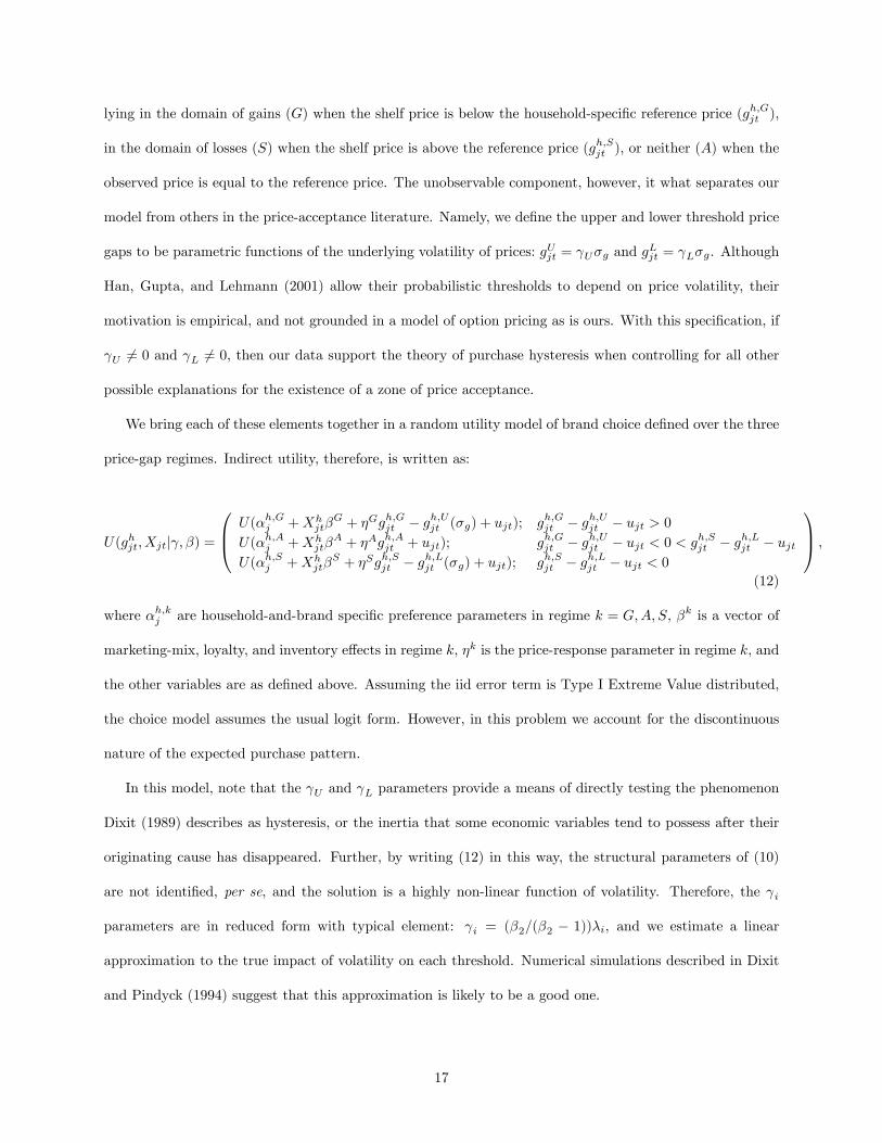
We bring each of these elements together in a random utility model of brand choice de�ned over the three

price-gap regimes. Indirect utility, therefore, is written as:

U(ghjt; Xjtj ; �) =

0B@ U(�h;Gj +Xhjt�

G + �Ggh;Gjt � gh;Ujt (�g) + ujt); gh;Gjt � gh;Ujt � ujt > 0U(�h;Aj +Xh

jt�A + �Agh;Ajt + ujt); gh;Gjt � gh;Ujt � ujt < 0 < gh;Sjt � gh;Ljt � ujt

U(�h;Sj +Xhjt�

S + �Sgh;Sjt � gh;Ljt (�g) + ujt); gh;Sjt � gh;Ljt � ujt < 0

1CA ;

(12)

where �h;kj are household-and-brand speci�c preference parameters in regime k = G;A; S, �k is a vector of

marketing-mix, loyalty, and inventory e¤ects in regime k, �k is the price-response parameter in regime k, and

the other variables are as de�ned above. Assuming the iid error term is Type I Extreme Value distributed,

the choice model assumes the usual logit form. However, in this problem we account for the discontinuous

nature of the expected purchase pattern.

In this model, note that the U and L parameters provide a means of directly testing the phenomenon

Dixit (1989) describes as hysteresis, or the inertia that some economic variables tend to possess after their

originating cause has disappeared. Further, by writing (12) in this way, the structural parameters of (10)

are not identi�ed, per se, and the solution is a highly non-linear function of volatility. Therefore, the i

parameters are in reduced form with typical element: i = (�2=(�2 � 1))�i, and we estimate a linear

approximation to the true impact of volatility on each threshold. Numerical simulations described in Dixit

and Pindyck (1994) suggest that this approximation is likely to be a good one.

17

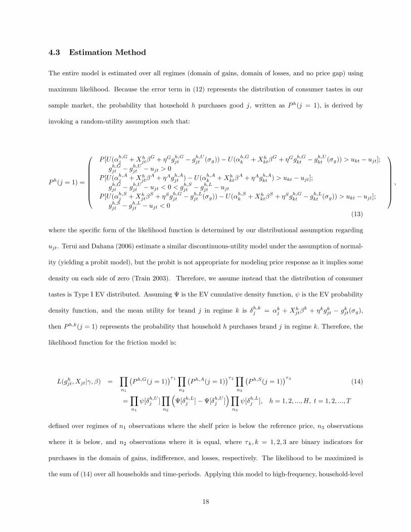
4.3 Estimation Method

The entire model is estimated over all regimes (domain of gains, domain of losses, and no price gap) using

maximum likelihood. Because the error term in (12) represents the distribution of consumer tastes in our

sample market, the probability that household h purchases good j, written as Ph(j = 1); is derived by

invoking a random-utility assumption such that:

Ph(j = 1) =

0BBBBBBB@

P [U(�h;Gj +Xhjt�

G + �Ggh;Gjt � gh;Ujt (�g))� U(�h;Gk +Xh

kt�G + �Ggh;Gkt � gh;Ukt (�g)) > ukt � ujt];

gh;Gjt � gh;Ujt � ujt > 0P [U(�h;Aj +Xh

jt�A + �Agh;Ajt )� U(�

h;Ak +Xh

kt�A + �Agh;Akt ) > ukt � ujt];

gh;Gjt � gh;Ujt � ujt < 0 < gh;Sjt � gh;Ljt � ujtP [U(�h;Sj +Xh

jt�S + �Sgh;Gjt � gh;Ljt (�g))� U(�

h;Sk +Xh

kt�S + �Sgh;Gkt � gh;Lkt (�g)) > ukt � ujt];

gh;Sjt � gh;Ljt � ujt < 0

1CCCCCCCA;

(13)

where the speci�c form of the likelihood function is determined by our distributional assumption regarding

ujt. Terui and Dahana (2006) estimate a similar discontinuous-utility model under the assumption of normal-

ity (yielding a probit model), but the probit is not appropriate for modeling price response as it implies some

density on each side of zero (Train 2003). Therefore, we assume instead that the distribution of consumer

tastes is Type I EV distributed. Assuming is the EV cumulative density function, is the EV probability

density function, and the mean utility for brand j in regime k is �h;kj = �kj + Xhjt�

k + �kgkjt � gkjt(�g);

then Ph;k(j = 1) represents the probability that household h purchases brand j in regime k: Therefore, the

likelihood function for the friction model is:

L(ghjt; Xjtj ; �) =Yn1

�Ph;G(j = 1)

��1Yn2

�Ph;A(j = 1)

��2Yn3

�Ph;S(j = 1)

��3 (14)

=Yn1

[�h;Uj ]Yn2

�[�h;Lj ]�[�h;Uj ]

�Yn3

[�h;Lj ]; h = 1; 2; :::;H; t = 1; 2; :::; T

de�ned over regimes of n1 observations where the shelf price is below the reference price, n3 observations

where it is below, and n2 observations where it is equal, where �k; k = 1; 2; 3 are binary indicators for

purchases in the domain of gains, indi¤erence, and losses, respectively. The likelihood to be maximized is

the sum of (14) over all households and time-periods. Applying this model to high-frequency, household-level

18

data on a speci�c grocery product, we are able to estimate the potentially persistent e¤ects of search costs

and retail price volatility on the existence and size of the latitude of price acceptance.

4.4 Operationalizing Utility Arguments

Operationalizing the model of utility that underlies our threshold model involves a number of constructs. In

each case, we adhere to the extant literature as closely as possible in order to di¤erentiate our model only

with the inclusion of the threshold term. In the econometric model above, we de�ne mean utility in regime

k for brand j as �h;kj = �kj +Xhjt�

k + �kgkjt � hl �g; where �kj are brand-speci�c preference parameters, Xhjt

are elements of the marketing mix which may or may not be unique to the household, gkjt is the price-gap

(reference price less shelf price) in regime k, hl ; l = G;S are the household-speci�c upper- and lower-price

thresholds that depend on the volatility of the gap term (�g). The speci�c variables that are included in the

matrix Xhjt are de�ned as follows:

pj = shelf-price of brand j,

feaj = a binary indicator variable that equals 1 when brand j is featured,

disj = a binary indicator variable that equals 1 when brand j is on display,

proj = a binary indicator variable that equals 1 when brand j is on promotion,

lphj = a binary indicator variable that equals 1 when household h purchased brand j on the last purchase

occasion,

blhj = a the within-household market share of brand j for household h;

invh = category inventory held by household h on the date of purchase,

sts = a binary indicator variable that equals 1 if the brand is purchased in store s.

Note that by including the shelf-price among the arguments of Xhjt;our maintained model is the "sticker-

shock" model of Winer (1986), Bell and Lattin (2000), and Chang, Siddarth, and Weinberg (1999). Among

the other variables, we calculate inventory in a relatively simple way. First, we use the entire data set to

calculate the average consumption rate (at the category level) of each household. We then estimate the initial

amount on hand from the observed consumption rate, and the date of the �rst purchase. We then calculate

a running inventory by adding new purchases, and subtracting consumption over the entire sample period.

We measure loyalty in two ways, following Han, Gupta, and Lehmann (2001). The �rst measure, lphj , is a

19

state-dependent measure that is de�ned in repeat-purchase terms. That is, a household is deemed loyal to a

speci�c brand if it is purchased on the previous shopping trip. The second measure, blhj ; is a cross-sectional

measure of brand loyalty in that it represents the share of brand j for household h calculated over a burn-in

period. For this purpose, we use the �rst 52 weeks of data. Each of these measures are well-accepted in the

reference-price literature (Mayhew and Winer 1992; Kalwani and Yim 1992).

Allowing the volatility parameter to vary randomly over households addresses the concern expressed by

Bell and Lattin (2000) that the sticker shock e¤ect is largely a result of failing to account for unobserved

household heterogeneity. Doing so also re�ects the probabilistic nature of thresholds captured by Han, Gupta,

and Lehmann (2001), but in a di¤erent way. In the utility model (12), the threshold parameters ( hU;L) are

modeled as random-normal variates: hl = l+� �h, where �h~N(0; 1): Because the hl parameter multiplies

the price-volatility term, the mean-threshold parameter, l, measures the extent to which volatility causes

the threshold price to widen or contract. Our primary hypothesis, therefore, is that l > 0, or that greater

volatility causes the threshold price to widen, and lower volatility reduces the threshold e¤ect. Of course,

ERthe validity of this hypothesis is conditional on the existence of reference prices around which thresholds

are formed.

Consumers form reference prices either according to an internal reference price (IRP), or external refer-

ence price (ERP) mechanism, or both (Rajendran and Tellis 1994; Bell and Bucklin 1999; Mazumdar and

Papatla 2000; Kopalle, and Lindsey-Mullikin 2003). If the consumer uses an IRP, then his or her notion of

what a product�s price should be is shaped by recent experience, memory, and expectations. On the other

hand, ERPs depend more on notions of what is reasonable in either a competitive sense, or as an absolute

"willingness-to-pay." Within both IRP and ERP, reference prices can be either "stimulus-based" if grounded

in a consumer�s current experience, or "memory-based" if grounded in previous experience with the brand

in question, or a rival brand (Briesh et al. 1997). Based on prior empirical research in similar categories,

we calculate reference prices using the brand-speci�c, last-purchase method that Briesch et al (1997) �nd to

be the preferred speci�cation and applied in a context similar to ours by Han, Gupta and Lehmann (2001).

That is, each household�s reference price for brand j is an exponentially-weighted average of the previous

reference price value, and the current shelf price:

20

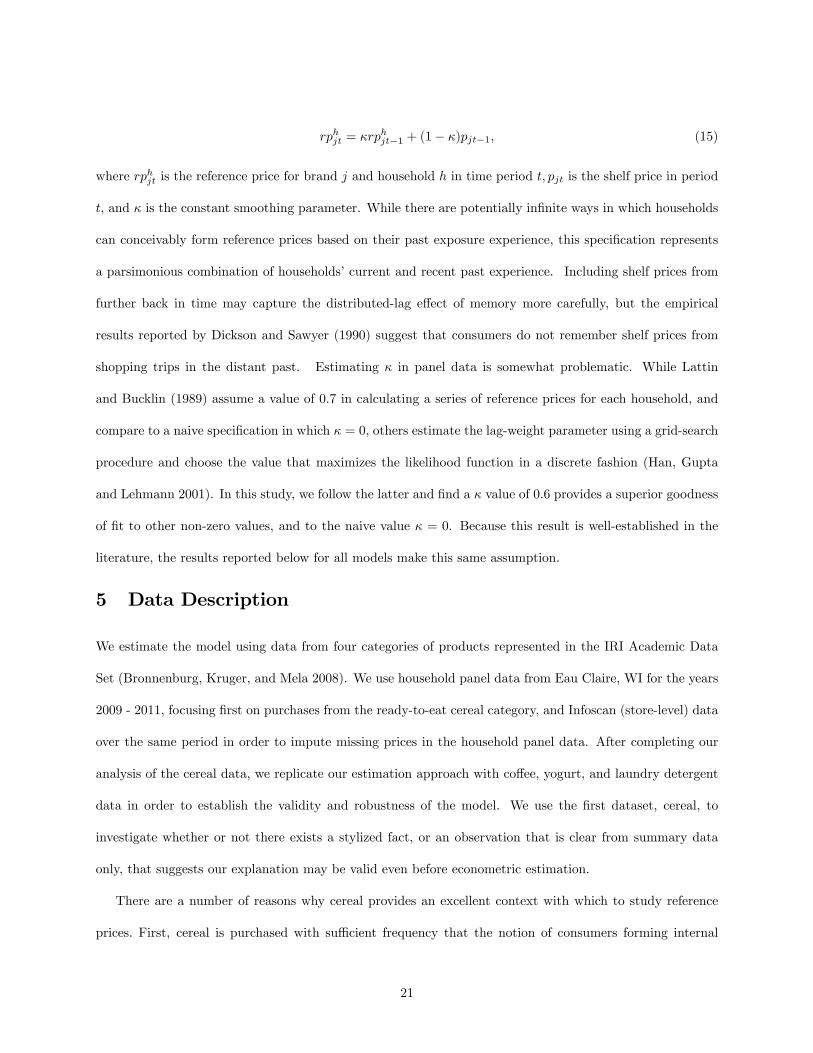
rphjt = �rphjt�1 + (1� �)pjt�1; (15)

where rphjt is the reference price for brand j and household h in time period t; pjt is the shelf price in period

t, and � is the constant smoothing parameter. While there are potentially in�nite ways in which households

can conceivably form reference prices based on their past exposure experience, this speci�cation represents

a parsimonious combination of households�current and recent past experience. Including shelf prices from

further back in time may capture the distributed-lag e¤ect of memory more carefully, but the empirical

results reported by Dickson and Sawyer (1990) suggest that consumers do not remember shelf prices from

shopping trips in the distant past. Estimating � in panel data is somewhat problematic. While Lattin

and Bucklin (1989) assume a value of 0.7 in calculating a series of reference prices for each household, and

compare to a naive speci�cation in which � = 0; others estimate the lag-weight parameter using a grid-search

procedure and choose the value that maximizes the likelihood function in a discrete fashion (Han, Gupta

and Lehmann 2001). In this study, we follow the latter and �nd a � value of 0:6 provides a superior goodness

of �t to other non-zero values, and to the naive value � = 0. Because this result is well-established in the

literature, the results reported below for all models make this same assumption.

5 Data Description

We estimate the model using data from four categories of products represented in the IRI Academic Data

Set (Bronnenburg, Kruger, and Mela 2008). We use household panel data from Eau Claire, WI for the years

2009 - 2011, focusing �rst on purchases from the ready-to-eat cereal category, and Infoscan (store-level) data

over the same period in order to impute missing prices in the household panel data. After completing our

analysis of the cereal data, we replicate our estimation approach with co¤ee, yogurt, and laundry detergent

data in order to establish the validity and robustness of the model. We use the �rst dataset, cereal, to

investigate whether or not there exists a stylized fact, or an observation that is clear from summary data

only, that suggests our explanation may be valid even before econometric estimation.

There are a number of reasons why cereal provides an excellent context with which to study reference

prices. First, cereal is purchased with su¢ cient frequency that the notion of consumers forming internal

21

reference prices is both intuitive and plausible. If consumers shop frequently, they are more likely to be

able to recall prices paid in the recent past (Briesch, et al. 1997). Further, cereal manufacturers introduce

new products every month, and o¤er frequent manufacturer promotions. Although frequent promotions can

reduce reference prices, the variation in retail prices they imply helps researchers identify behavior when

prices change either above the reference price or below. Third, the cereal category is dominated by two

manufacturers, Kelloggs and General Mills, who are well-known to behave strategically through both prices

and product introductions (Nevo 2001). When there is a closely-competitive product for consumers to switch

into, the notion of a "kinked demand curve" is more likely to arise. Fourth, cereal is an important category

to retailers, so tends to re�ect a retailers�overall pricing strategy. If a retailer claims to operate some form

of everyday-low-price (EDLP) strategy, then cereal prices will generally be lower and more stable than at

other retailers. Stable prices, of course, are more conducive to consumers�forming reference prices based on

their own memories. In sum, if consumers do indeed form reference prices for frequently-purchased consumer

packaged goods, then cereal is likely a good context in which they will be revealed.

In panel data, it is necessary to have data on prices for not only the product that was purchased, but

those that were not purchased as well. Both the household-purchase and store-level contains a masked store

code that allowed us to merge both data sets by store, week, and UPC. By combining the household and

store-level data sets, we observe the complete set of prices, and other marketing mix variables, for all UPCs

available on a given purchase trip. We include only households who purchase cereal from the two most

popular stores in the data set because the other stores do not provide price information to IRI, so we are

unable to impute price for non-purchased items in a consistent way. The resulting merged data set provides

su¢ cient variation in prices and choice probabilities across brands and over time in order to identify the

reference-price mechansisms we investigate (see tables 1 and 2).

[tables 1 and 2 in here]

Household data is necessary for our analysis because we model household-speci�c reference prices, and

require household-level choice-variation to identify the model. While tables 1 and 2 provide aggregated-

evidence in support of variation in choice probabilities, table 3 shows the characteristics of the households

in our sample. The data in this table reveals that our sample skews slightly higher in mean income relative

22

to the U.S. average, and exhibits less racial diversity than a more general sample would, but the Eau Claire

data are nonetheless well-accepted for quantitative analyses such as the one we present here.

[table 3 in here]

If reference prices are indeed a feature of the data, they should be apparent from simply examining

price data and the associated sales volumes. If small changes in the price of a particular brand are met

with only small changes in volume, but larger changes induce substantial changes, then this would provide

evidence for the existence of reference prices, if not volatility-induced price thresholds. Table 4 presents

stylized facts employing the twenty cereal brands in the study for the years 2009�2011. The table illustrates

switching behavior of consumers as they face small gains/losses (i.e., the reference price is relatively close

to the prevailing retail price), as well as relative large losses and gains (i.e. large negative and positive

distances between reference and retail prices). The table indicates that consumers are quite unlikely to

change behavior when they face small gains or losses. When losses are small, in average, only 3.0 percent of

consumers stop purchasing brand i. In contrast, when losses are relatively large, 15.7 percent of consumers

switch to alternative brands, in average. The di¤erences in consumer response are more considerable in

the realm of gains (i.e. when reference prices are greater than retail prices). When gains are small, in

average, only 2.4 percent of consumers switch to purchase brand i; whereas, in average, 19.9 percent of

consumers switch to brand i when gains are relatively large. These stylized facts indicate di¤erences across

brands, probably due to such factors as brand loyalty and frequency of purchase, among others. Although

these summary results are suggestive of reference-price behavior, we can only isolate the speci�c e¤ect of

reference prices if all other marketing-mix, and unobserved factors, are properly taken into account in the

more complete econometric model econometric model. In the next section, we present the results obtained

from estimating our model.

[table 4 in here]

6 Results and Discussion

We �rst present and interpret the results obtained with data from our focal category �ready-to-eat cereal

�and then compare the results from our maintained model with estimates from other categories, and from

23

other, plausible alternatives.

6.1 Estimation Results

The sticker shock model maintains that shelf prices will continue to have a negative e¤ect on utility, even

when reference prices are appropriately taken into account. And, de�ned as we do here, the price-gap term

should be positively related to utility as reductions in the shelf price below the reference price represent

bene�ts for the consumer. Our version of the sticker shock model further maintains that the price-gap term

must reach a certain value before consumers change their behavior. We specify this threshold term as a

function of the variance of the price-gap variable. In table 5, the left-most four columns show the estimation

results for the base sticker shock model that includes price-thresholds, but does not allow for unobserved

heterogeneity (Model 1). In this model, we see that each of the sticker-shock parameters are of the expected

sign and signi�cantly di¤erent from zero. Most importantly, the threshold parameter estimates suggest that

consumers require shelf prices to rise signi�cantly above the reference price before changing their behavior, or

fall signi�cantly below, and that the size of this "latitude of acceptance" widens in the volatility of the price-

gap. Indeed, the threshold parameter estimates in table 5 imply a region of between $0.151 / oz and $0.267

/ oz wherein consumers� response to variations in the reference remains the same. In other words, when

consumers are in the domain of gains, or when the shelf-price falls below the reference price, consumers do

not alter their behavior until a shelf price of $0.151 / oz is reached. On the other hand, when they are in the

domain of losses, they do not respond until an upper-threshold price of $0.267 / oz is reached. These initial

results also support the predictions of Prospect Theory (Kahneman and Tversky 1979) as the magnitude of

the Gain / Loss parameter is larger when consumers are in the domain of losses than in the domain of gains.

These results, however, assume there is no unobserved heterogeneity in response to variations in either price

or price-gap volatility.

[table 5 in here]

Accounting for heterogeneity in volatility-response has a signi�cant impact on our parameter estimates,

but not in the same qualitative way as others have found (Bell and Lattin 2000). Based on a likelihood ratio

(LR) speci�cation test, accounting for unobserved heterogeneity in response to reference-price volatility

improves the �t substantially (Model 2 in table 5). With two degrees of freedom the critical chi-square

24

test statistic for a LR test between Model 1 and Model 2 is 5.991, while the calculated test statistic value

comparing the two models is 1,523.16. Unlike Bell and Lattin (2000), we �nd that including this source of

heterogeneity does not weaken the reference-price e¤ect. In fact, the latitude of price acceptance is larger

with this model than the �xed-coe¢ cient version as the gap now widens to $0.152 / oz to $0.279 / oz. In

terms of the relevant point-estimates, we �nd that the price-gap term in the domain of gains is only slightly

attenuated (2.217 compared to 2.255) while in the domain of losses, it is considerably smaller (2.507 versus

2.698). However, the volatility-e¤ect estimate falls to 24.414 compared to 25.045 in the domain of gains, and

rises to 31.908 relative to 26.966 in the domain of losses. It is this e¤ect that is primarily responsible for the

dramatic widening in the latitude of price acceptance. In the sticker-shock model, however, it is assumed

that consumers respond to not only di¤erences between their reference price and the observed shelf price,

but the level of shelf prices as well. Therefore, it is reasonable to assume heterogeneity in response to shelf

prices as well.

Model 3 in table 5 presents the results from estimating a model that accounts for heterogeneity in both

the response to price volatility and shelf prices. Again comparing models 2 and 3 using a LR test, we

�nd a calculated chi-square statistic of 6,228.36 relative to the same critical chi-square statistic of 5.991.

Therefore, we prefer Model 3 to either Model 2 or Model 1 and conclude that both sources of heterogeneity

are important. Compared to the previous models, however, we �nd a latitude of price acceptance closer to

Model 1 �the model that did not account for heterogeneity �than in Model 2. Speci�cally, the lower shelf-

price threshold in the domain of gains is now $0.151 / oz, while the upper threshold is $0.270 / oz. While the

mean price-volatility parameter in the domain of gains rises slightly to 25.009, the corresponding parameter

estimate in the domain of losses falls to 28.164. Estimates of the price-gap parameter are also closer to

those in Model 1, which suggests that the direction of bias induced by failing to account for heterogeneity

in price-response is opposite the direction of bias caused by not allowing for heterogeneity in response to

volatility. Again, it is di¢ cult to say that the presence of heterogeneity weakens the reference-price e¤ect.

Similar to Model 1, this preferred model also provides evidence in support of the predictions of Prospect

Theory as the magnitude of the response to price-gaps is larger when consumers are in the domain of losses

relative to the domain of gains.

25

With these estimation results, we are able to address the question raised by Pauwels, Srinivasan and

Franses (2007). Namely, they are concerned with whether reference prices and response thresholds are an

artefact of household-level data, or whether they can be expected to arise in aggregate data as well? While

most of the empirical analyses of this question use household-level data, where threshold behavior is appar-

ent even from casual inspection, many market analysts work with aggregate data, and still operate on the

assumption that price-response is subject to threshold-like behavior. Because we are able to explicitly esti-

mate threshold parameters with our friction-model approach, and the distribution of consumer heterogeneity

that governs the location of the thresholds, we examine whether they are likely to be apparent in aggregate,

store-level data by simulating empirical threshold values. We analyze these simulated data in two ways in

order to determine whether there is any evidence of threshold behavior �one qualitative and another more

quantitative.

First, �gure 1 shows the simulated data for one brand (General Mills Cheerios) over the sample period.

The �gure shows the position of the upper and lower thresholds implied by our estimates for this brand,

the observed price, and the ratio of the implied market share among consumers who are in the domain of

gains (shelf price below their reference price) to those who are in the domain of losses (shelf price above the

reference price). While the aggregated shares necessarily show considerable variation from week to week,

some patterns are in evidence. Namely, when the observed price goes above the upper threshold, consumers

in the domain of losses appear to respond by reducing their purchases, and the relative share among those

in the domain of gains rises (see weeks 117 - 145). Consumers who are in the domain of gains have relatively

high reference prices (for the same shelf price, they perceive the price to be relatively low) so when the price

falls below the lower threshold, consumers in the domain of losses are induced into the market, and their

relative share rises. Although this graphical analysis is suggestive of threshold-type behavior among two

groups of consumers, it is not de�nitive.

[�gure 1 in here]

Second, we use the simulated aggregate data to estimate simple models of threshold price behavior for

each brand. From a practitioner�s perspective, price-thresholds exist when the response elasticity di¤ers in a

meaningful away above and below a certain price level. We use the price thresholds in �gure 1 to de�ne these

26

regions, and estimate simple own-price elasticities above and below the threshold price levels. We show the

estimation results from a sample of 10 brands in table 6. These results show that, in each case, the aggregate

price elasticity di¤ers signi�cantly between consumers in the domain of gains relative to those in the domain

of losses. In particular, the response elasticity is lower (in absolute value) when the shelf price is below the

lower threshold (domain of gains), relative to when the price is above the upper threshold (domain of losses).

As with the household-level estimates, these �ndings support the predictions of Prospect Theory (Kahneman

and Tversky 1979) and suggest that consumers are more sensitive to variations in price when experiencing

losses, than when they perceive observed price to be o¤ering "a good deal." From a revenue-management

perspective, these �ndings are also interesting in that the gains-elasticity is uniformly below 1.0 (in absolute

value) and the loss-elasticity is above 1.0. This outcome suggests that retailers can increase revenue by

raising shelf prices when the "aggregate consumer" perceives himself to be in a positive position, and can

increase revenue by reducing shelf prices when the representative consumer perceives losses. This is neither

shocking nor counter-intuitive, but does provide a formal empirical rationale for sound retailing behavior.

[table 6 in here]

6.2 Comparison to Alternative Models

We compare the �t of our maintained model against three alternatives. To ensure the comparison is valid,

however, we restrict our attention to the class of models that explicitly account for the multiple-regime nature

of the threshold model. Because models that do not control for the censored nature of the data that is implied

by threshold behavior are fundamentally inconsistent, any comparison between our model and a single-regime

model would be comparing apples and oranges. Maintaining the multiple-regime structure implied by the

threshold model, the primary di¤erences between our utility model and others in the literature (Lattin and

Bucklin 2001; Han, Gupta, and Lehmann 2001) are the inclusion of the shelf price in addition to the price-gap

term (the "sticker-shock" model), modeling price-thresholds as dependent upon price volatility, and allowing

for unobserved heterogeneity in the size of the thresholds. Therefore, the �rst alternative contains neither the

sticker-shock term, volatility, nor unobserved heterogeneity. In the second alternative, we include a volatility

term, but not the sticker-shock term or unobserved heterogeneity. In the third, we allow for unobserved

heterogeneity. We also estimated �xed-coe¢ cient and random coe¢ cient versions of the three-regime sticker

27

shock model (see table 5), in addition to one in which both thresholds and price-response are random

parameters. Because these models are nested, we compare the goodness-of-�t using standard likelihood-

ratio tests. We also estimate the preferred two-regime speci�cation in three other categories (yogurt, co¤ee,

and laundry detergent) in order to examine the robustness of our results across di¤erent product categories.

In table 7, we show estimation results obtained from models that do not include the shelf-price term,

but do include various forms of the price-gap volatility term that forms the core of our maintained model.

The �rst two models (Models 4 and 5) compare the �t of a non-sticker-shock model that includes price-

gap volatility (Model 5) with one that does not (Model 4). With a calculated LR statistic of 3,719.22, we

easily reject Model 4 in favor of the alternative. Combined with the individual signi�cance of the threshold-

volatility terms in Model 5, we conclude that Model 5 provides a better �t to the data. Next, we compare

Model 5 to an alternative that accounts for unobserved heterogeneity in the location of the price thresholds

(Model 6). The LR statistic for this comparison is 7,682.32, so we again favor the random-coe¢ cient to the

�xed-coe¢ cient variant. Consistent with the results reported in table 5, but contrary to Bell and Lattin

(2000), including heterogeneity causes the Gain / Loss terms to become more statistically signi�cant, albeit

slightly smaller in magnitude. Finally, we compare the preferred non-sticker-shock speci�cation (Model 6)

to the preferred sticker-shock alternative. Again using a LR test, we �nd a calculated chi-square statistic of

506.40, which suggests that the best sticker-shock model provides a better �t to the data than a comparable

model that does not include both the price-gap and shelf-price.

[table 7 in here]

In table 8, we present estimation results from categories that are more frequently purchased than cereal

(yogurt) and less frequently purchased (co¤ee and laundry detergent). Reference price-response is likely

to be relatively sensitive to frequency of purchase (or the wavelength of the purchase cycle) because our

reference-price mechanism is based on the consumer�s ability to recall the price paid on the focal brand at

the last purchase occasion. The longer the time since last purchase, the less likely the consumer is to be

able to recall the price paid. For all three categories, we present estimates from our maintained sticker-shock

speci�cation that accounts for heterogeneity in response to both price and price-gap volatility. Again, our

key parameter estimates are the price-gap responses and estimated threshold (volatility) parameters. In each

28

case, the estimates in table 8 show that the price-gap term has a positive e¤ect whether households are in

the domain of gains or losses, and that the marginal e¤ect di¤ers signi�cantly between regimes. Finding

that the price-gap is not statistically signi�cant in the "gain" regime for co¤ee and detergent supports

the conjecture that consumers have a more di¢ cult time forming reference prices for relatively long-cycle

products. Moreover, the asymmetry of this outcome lends further support to the notion that consumers

behave in fundamentally di¤erent ways when experiencing gains instead of losses. While they do not appear

to care whether shelf prices fall below their reference price, their behavior changes signi�cantly when shelf

prices rise above reference prices. Further, the location of the implied threshold e¤ect depends on the

volatility of the price-gap term, con�rming the real-option hypothesis maintained throughout. That is, the

size of the latitude of acceptance between the upper and lower price-thresholds appears to widen in the

variability of the di¤erence between reference and shelf prices.

[table 8 in here]

6.3 Implications

These results support the hypothesis that consumers appear to respond to not only shelf prices, but also

to the di¤erence between shelf prices and some notion of what the price of a product "should be." More

speci�cally, they behave as if there are thresholds around this reference price that induce fundamentally

di¤erent behavior depending upon whether shelf prices rise above the upper threshold, or fall below the

lower threshold. While these insights are not unique, we also show that these thresholds are driven largely

by the existence of a real option that consumers are reluctant to exercise too early, or too late.

Our �ndings have important implications for both research in this area and marketing of consumer

packaged goods in general. First, while others include price-volatility as an argument of threshold functions

in empirical models similar to ours (Han, Gupta, and Lehmann 2001, for example) we o¤er a theoretical

explanation and an empirical approach that is grounded in threshold-price behavior. The importance of

this advance is less in the technical details of the econometric model, but that we o¤er an explanation

for consumer behavior that is grounded in rational, optimizing behavior and not in a violation of rational

economic behavior. This �nding suggests that apparent violations of economic rationality may not necessarily

be due to pathological consumer behavior, but rather the failure to adequately model the complexity of the

29

decision process.

Second, from a practitioner�s standpoint our �ndings suggest that price thresholds are indeed important,

and that the latitude of price acceptance around reference prices is relatively large. This, in turn, means

that retailers have some cover in changing prices for frequently-purchased goods when the cost of search is

high, and prices volatile, but the cost of exceeding either the upper or lower price threshold is higher than

previously believed in terms of lost revenue.

Third, our �ndings suggest that there is some scope for strategic obfuscation on the part of retailers

(Ellison and Ellison 2009). Although it is well understood that frequent promotions can erode brand equity,

inducing price variability can widen the latitude of price acceptance, providing retailers more �exibility to

change prices before consumers will notice changes in the shelf price.

Fourth, although our model is grounded in optimizing economic behavior, our �ndings are fully consistent

with the behavioral theories of Kahneman and Tversky (1979) in that consumers appear to be more averse

to retail prices rising above their upper threshold than they are appreciative of prices that fall below their

lower threshold. In some sense, this �nding provides both theoretical and empirical support for the kinked

demand curve of Sweezy (1939) and has dramatic e¤ects on retailer pricing strategies (Kopalle, Rao, and

Assungdo 1996). If demand is more elastic above the upper threshold than it is below the lower threshold,

then aggregate demand curves will exhibit a "kink" around the reference price. The reference price then

becomes a natural choice for rival retailers to regard as the industry-standard price, and a focal point for

tacitly collusive pricing behavior. Moreover, von Massow and Hassini (2013) show that threshold-price

behavior can generate cyclical optimal price-paths, as opposed to a single-price policy.

7 Conclusion

In this paper, we document a new explanation for the existence of threshold e¤ects in consumers�purchases

of consumer packaged goods. If consumers face a �xed cost of search, and if retail prices are volatile around

consumers�reference prices, then their shopping decisions will embody a real option. A real option implies

that consumers will rationally wait for observed prices to either rise above an upper threshold or fall below a

lower threshold before exercising their option to respond to an observed price change. These thresholds form

30

a zone of inaction that has been described as the latitude of price acceptance in the behavioral literature. As

a behavioral construct, price acceptance depends on idiosyncractic behavior that may be di¢ cult to exploit

from a practical perspective. Rather, our theory suggests that the zone of inaction widens in the volatility

of retail prices, or more precisely the di¤erence between retail prices and consumers�reference prices, so can

be used by retailers to set prices strategically.

We test our theory of threshold price behavior using an extension of the friction model of Rosett (1959)

that accounts for unobserved household heterogeneity and extreme-value errors. Rather than segment the

price-response term in a traditional model of brand choice, our econometric model explicitly recognizes the

censored nature of data generated by threshold-price behavior. We estimate our econometric model using

household-level data from the cereal, yogurt, co¤ee, and detergent categories. In each case, we �nd evidence

in support of reference price behavior, and support for the real option explanation for the existence of

threshold prices. Because retailers are generally more concerned with aggregate behavior than individual

choices, we show that our �ndings aggregate out to the market level, and that our �ndings are not an

artefact of focusing only on household behavior. In this sense, our model provides an operational tool that

practitioners can exploit to improve pricing strategy.

There are many implications that follow from these results, but perhaps the most important concern the

opportunity a¤orded retailers to price strategically. Inaction by consumers implies that they assimilate price

changes into a pattern of perceived "normal" prices, an assimilation process that is economically-optimal

according to the theory advanced here, and do not change their behavior in a signi�cant way. If retailers are

able to estimate the location of the thresholds beyond which consumers no longer assimilate price changes,

they can raise prices up to a point just below the upper threshold, and maximize revenue without losing

tra¢ c. If all retailers price this way, then a common price point can arise in a way that is observationally

equivalent to tacit collusion. Hysteretic behavior on the part of consumers, therefore, represents a source of

retail market power that has not been previously identi�ed. Retailers can exploit this form of market power

by either raising search costs, or causing prices to become more volatile over time.

Future research in this area may extend our approach to products other than consumer packaged goods.

Consumer durables, for example, represent purchases that are more discrete, lumpy, and a longer-term

31

commitment of household resources. For these reasons, the real option phenomenon described here is likely

to be more signi�cant for consumer durables than for consumer packaged goods. Because the zone of

inaction induced by price variability rises in both volatility and the cost of search, categories that are subject

to relatively high search costs may also exhibit sharper threshold results than those shown here. Healthcare

insurance, retirement plans, and other inherently complicated products are likely to exhibit relatively wide

pricing thresholds.

32

References

[1] Bell, D. R. and R. E. Bucklin. 1999. "The Role of Internal Reference Price in the Category Purchase

Decision." Journal of Consumer Research 26: 128-43.

[2] Bell, D. R., J. M. Lattin. 2000. �Looking for Loss Aversion in Scanner Data: The Confounding E¤ect

of Price Response Heterogeneity.�Marketing Science 19: 185-200.

[3] Boztug, Y. and L. Hildebrandt. 2005. �An Empirical Test of Theories of Price Valuation Using a Semi-

Parametric Approach, Reference Prices, and Accounting for Heterogeneity. �SFB 649 Discussion Paper

2005-057.

[4] Briesch, R. A., L. Krishnamurthi, T. Mazumdar, and S . P. Raj. 1997. �A Comparative Analysis of

Reference Price Models.�Journal of Consumer Research 24: 202-214.

[5] Bronnenberg, B. J., M. W. Kruger, and C. F. Mela. 2008. "Database Paper: The IRI Marketing Data

Set." Marketing Science 27: 745-748.

[6] Caballero, R. and E. Engel. 1999. �Explaining Investment Dynamics in U.S. Manufacturing: A Gener-

alized (S, s) Approach.�Econometrica 67: 783-826.

[7] Cecchetti, G. 1986. �The Frequency of Price Adjustment: A Study of Newsstand Prices of Magazines.�

Journal of Econometrics 31: 255-274.

[8] Chang, K., S. Siddarth, and C. B. Weinberg. 1999. �The Impact of Heterogeneity in Purchase Timing

and Price Responsiveness on Estimates of Sticker Shock E¤ects.�Marketing Science 18: 178-192.

[9] Choi, S., S-J. Park, C. Qiu, and M. Stanyer. 2013. �The Discount is Unfair: Egocentric Fairness in

Risky Discounts. �Journal of Economic Psychology 39: 32.

[10] De Los Santos, B., A. Hortacsu and M. R. Wildenbeest. 2012. "Testing Models of Consumer Search

Using Data on Web Browsing and Purchasing Behavior." American Economic Review 102: 2955-2980.

33

[11] Della Bitta, A. J., and K. B. Monroe. 1974. �The In�uence of Adaptation Levels on Subjective Price

Perceptions. �In Advances in Consumer Research Volume 1, S. Ward and P. Wright (eds.), Ann Abor,

MI: Association for Consumer Research: 359-369.

[12] Dickson, P. R., and A. G. Sawyer. 1990. "The Price Knowledge and Search of Supermarket Shoppers."

The Journal of Marketing 54: 42-53.

[13] Dixit, A. K. 1989. �Entry and Exit Decisions Under Uncertainty.� Journal of Political Economy 97:

620-638.

[14] Dixit, A. K. 1992. �Investment and Hysteresis.�Journal of Economic Perspectives 6: 107-132.

[15] Dixit, A. K. and R. S. Pindyck. 1994. Investment Under Uncertainty. Princeton, N.J.: Princeton Uni-

versity Press.

[16] Edwards, K. D. 1996. �Prospect Theory: A Literature Review. � International Review of Financial

Analysis 5: 19�38.

[17] Eichenbaum, M., N. Jaimovic and S. Rebelo. 2011. �Reference Prices and Nominal Rigidities.�American

Economic Review 101: 234-262.

[18] Ellison, G., and S. F. Ellison. 2009. �Search, Obfuscation and Price Elasticities on the Internet.�Econo-

metrica 77: 427-452.

[19] Emery, F. 1969. �Some Psychological Aspects of Price. � In Pricing Strategy, B. Taylor and G. Wills

(eds). London: Staples.

[20] Erdem, T., G. Mayhew, and B. Sun. 2001. "Understanding Reference-Price Shoppers: A Within- and

Cross Category Analysis." Journal of Marketing Research 38: 445-58.

[21] Estelami, H., D. R. Lehmann, and A. C. Holden. 2001. �Macro-economic Determinants of Consumer

Price Knowledge: a Meta-analysis of Four Decades of Research. �International Journal of Research in

Marketing 18: 341-355.

34

[22] Gopinath, G., P. -O. Gourinchas, C. -T. Hsieh, and N. Li. 2011. �International Prices, Costs, and

Markup Di¤erences.�American Economic Review 101: 2450-2486.

[23] Gotlieb, J. B., and A. J. Dubinsky, Alan. 1991. �In�uence of Price on Aspects of Consumers�Cognitive

Process. �Journal of Applied Psychology 76: 541.

[24] Gupta, S., and L. G. Cooper. 1992. �Discounting of Discounts and Promotion Thresholds.�Journal of

Consumer Research 19: 401-411.

[25] Gurevich, G., D. Kliger, and O. Levy. 2009. �Decision-Making under Uncertainty: A Field Study of

Cumulative Prospect Theory. �Journal of Banking and Finance 33: 1221-1229.

[26] Han, S., S. Gupta, and D. R. Lehmann. 2001. �Consumer Price Sensitivity and Price Thresholds. �

Journal of Retailing 77: 435�456.

[27] Hardie, B. G. S., E. J. Johnson, and P. S. Fader. 1993. "Modeling Loss Aversion and Reference Depen-

dence E¤ects on Brand Choice." Marketing Science 12: 378�394.

[28] Helson, H. 1964. Adaptation-Level Theory. New York: Harper and Row Publishers, Inc.

[29] Henderson, V. 2012. �Prospect Theory, Liquidation, and the Disposition E¤ect. �Management Science

58: 445-460.

[30] Hong, H. and M. Shum. 2006. "Using Price Distributions to Estimate Search Costs." RAND Journal of

Economics 37: 257-275.

[31] Janiszewski, C., and D. R. Lichtenstein. 1999. �A Range Theory Account of Price Perception. �Journal

of Consumer Research 25: 353-368.

[32] Kahneman, D. and A. Tversky. 1979. "Prospect Theory: An Analysis of Decision Under Risk." Econo-

metrica 47: 263-291.

[33] Kalwani, M. U., and C. K. Yim. 1992. �Consumer Price and Promotion Expectations: An Experimental

Study.�Journal of Marketing Research 29: 90-100.

35

[34] Kalyanaram, G., and J. D. C. Little. 1994. �An Empirical Analysis of Latitude of Price Acceptance in

Consumer Package Goods.�Journal of Consumer Research 21: 408-418.

[35] Kalyanaram, G., and R. S. Winer. 1995. �Empirical Generalizations from Reference Price Research.�

Marketing Science 14: G161-G169.

[36] Kim, J. B., P. Albuquerque, and B. J. Bronnenberg. 2010. "Online Demand Under Limited Consumer

Search." Marketing Science 29: 1001-1023.

[37] Kinard, B., M. L. Capella, and G. Bonner. 2013. �Odd Pricing E¤ects: An Examination Using

Adaptation-Level Theory. �The Journal of Product and Brand Management 22: 87-94.

[38] Klein, N. M., and J. E. Oglethorpe. 1987. �Cognitive Reference Points in Consumer Decision Making.

� In Advances in Consumer Research, M. Wallendorf and P. Anderson (eds.), Provo: UT Association

for Consumer Research.

[39] Kopalle, P., and J. Lindsey-Mullikin. 2003. "The Impact of External Reference Price on Consumer Price

Expectations." Journal of Retailing 79: 225-36.

[40] Kopalle, P., A. G. Rao, and J. Assungdo. 1996. "Asymmetric Reference Price E¤ects and Dynamic

Pricing Policies." Marketing Science 15: 60-85.

[41] Kumar, V., K. Karande, and W. J. Reinartz. 1998, �The Impact of Internal and External Reference

Prices on Brand Choice: the Moderating Role of Contextual Variables. �Journal of Retailing 74: 401-

425.

[42] Lattin, J. M., and R. E. Bucklin. 1989. �Reference E¤ects of Price and Promotion on Brand Choice

Behavior.�Journal of Marketing Research 26: 299-310.

[43] Levy, H., and Z. Wiener. 2013. �Prospect Theory and Utility Theory: Temporary versus Permanent

Attitude toward Risk. �Journal of Economics and Business 68: 1-23.

[44] Lichtenstein, D. R., and W. O. Bearden. 1989. �Contextual In�uences on Perceptions of Merchant-

Supplied Reference Prices. �Journal of Consumer Research 16: 55�66.

36

[45] Loughran, T., and B. McDonald. 2013. �IPO First-Day Returns, O¤er Price Revisions, Volatility, and

Form S-1 Language. �Journal of Financial Economics 109: 307-326.

[46] Maddala, G. S. 1983. Limited-Dependent and Qualitative Variables in Econometrics Econometric Soci-

ety Monographs No. 3 Cambridge University Press: Cambridge, UK.

[47] Management Science Associates, Inc. Price Elasticity (http://www.msa.com/analysis/pricing/price.htm).

November 22, 2013.

[48] Mayhew, G. E., and R. S. Winer. 1992. �An Empirical Analysis of Internal and External Reference

Price Using Scanner Data.�Journal of Consumer Research 19: 62-70.

[49] Mazumdar, T., S. P. Raj, and I. Sinha. 2005. �Reference Price Research: Review and Propositions.�

Journal of Marketing 69: 84-102.

[50] Mazumdar, T., and S. Y. Jun. 1992. �E¤ects of Price Uncertainty on Consumer Purchase Budget and

Price Thresholds.�Marketing Letters 3: 323-329.

[51] Mazumdar, T. and P. Papatla. 2000. "An Investigation of Reference Price Segments." Journal of Mar-

keting Research 37: 246�259.

[52] Mehta, R., S. Rajiv and K. Srinivasan. 2003. "Price Uncertainty and Consumer Search: A Structural

Model of Consideration Set Formation." Marketing Science 22: 58-84.

[53] Monroe, K. B. 1971. �Measuring Price Thresholds by Psychophysics and Latitudes of Acceptance. �

Journal of Marketing Research 8: 460�64.

[54] Moraga-Gonzalez, J. L. and M. R. Wildenbeest. 2008. "Maximum Likelihood Estimation of Search

Costs." European Economic Review 52: 820-848.

[55] Nevo, A. 2001. "Measuring Market Power in the Ready-to-Eat Cereal Industry." Econometrica 69:

307-342.

[56] Pauwels, K. H., P. H. Franses, and S. Srinivasan. 2004. �Reference-based Transitions in Short-run Price

Elasticity. �ERIM Report Series Reference No. ERS-2003-095-MKT.

37

[57] Pauwels, K., S. Srinivasan, and P. H. Franses. 2007. �When do Price Thresholds Matter in Retail

Categories?�Marketing Science 26: 83-100.

[58] Putler, D . 1992. �Incorporating Reference Price E¤ects into a Theory of Consumer Choice.�Marketing

Science 11: 287-309.

[59] Rajendran, K. N., and G. J. Tellis. 1994. �Contexual and Temporal Components of Reference Price.�

Journal of Marketing 58: 22-34.

[60] Raman, K., and F. M. Bass. 2002. �A General Test of Reference Price Theory in The Presence of

Threshold E¤ects. �Tijdschrift voor Economie en Management 47: 205�226.

[61] Roberts, J. H., J. M. Lattin. 1991. "Development and Testing of a Model of Consideration Set Compo-

sition." Journal of Marketing Research 28: 429-440.

[62] Rosett, R. N. 1959. "A Statistical Model of Friction in Economics." Econometrica 27: 263-67.

[63] Sawyer, A. G., and P. R. Dickson.1984. �Psychological Perspectives on Consumer Response to Sales

Promotion. �In Research on Sales Promotion: Collected Papers, Katherine E. Jocz, (ed.) Cambridge,

MA: Marketing Science Institute.

[64] Sherif, C. W. 1963. "Social Categorization as a Function of Latitude of Acceptance and Series Range."

The Journal of Abnormal and Social Psychology 67: 148-156.

[65] Sherif, M., and C. I. Hovland.1961. Social Judgment. New Haven: Yale University Press.

[66] Sheshinski, E. and Y. Weiss. 1977. �In�ation and the Costs of Price Adjustment.�Review of Economic

Studies 44: 287-303.

[67] Simon, J. 1969. "A Further Test of the Kinky Oligopoly Demand Curve." American Economic Review

59: 971-975.

[68] Slade, M. E. 1998. �Optimal Pricing with Costly Adjustment: Evidence from Retail-Grocery Prices.�

Review of Economic Studies 65: 87-107.

38

[69] Slade, M. E. 1999. �Sticky Prices in a Dynamic Oligopoly: An Investigation of (s, S) Thresholds.�

International Journal of Industrial Organization 17: 477-511.

[70] Stigler, G. 1947. "The Kinky Oligopoly Demand Curve and Rigid Prices." Journal of Political Economy

55: 432-449.

[71] Sweezy, P. 1939. "Demand Under Conditions of Oligopoly." Journal of Political Economy 47: 568-573.

[72] Terui, N., and W. D. Dahana. 2006. �Research Note �Estimating Heterogeneous Price Thresholds.

Marketing Science 25: 384-391.

[73] Train, K. 2003. Discrete Choice Methods with Simulation. Cambridge University Press, Cambridge,

UK.

[74] Tversky, A., and D. Kahneman.1981. �The Framing of Decisions and the Psychology of Choice. �Science

211: 453�58.

[75] Urbany, J. E., and P. R. Dickson.1990. �Prospect Theory and Pricing Decisions. �Journal of Behavioral

Economics 19: 69�81.

[76] von Massow, M., and E. Hassini. 2013. �Pricing Strategy in the Presence of Reference Prices with

Thresholds.�Journal of Revenue Pricing Management 12: 339-359.

[77] Wildenbeest, M. R. 2011. "An Empirical Model of Search with Vertically Di¤erentiated Products."

RAND Journal of Economics 42: 729-757.

[78] Willis, J. L. 2000. �Estimation of Adjustment Costs in a Model of State-Dependent Pricing.�Research

Division Working Paper, Federal Reserve Bank of Kansas City. December.

[79] Winer, R. 1986. �A Reference Price Model of Brand Choice for Frequently Purchased Products.�Journal

of Consumer Research 13: 250-256.

39

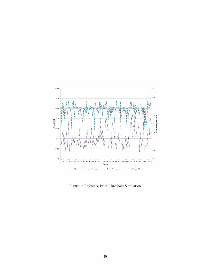
Figure 1: Reference Price Threshold Simulation

40

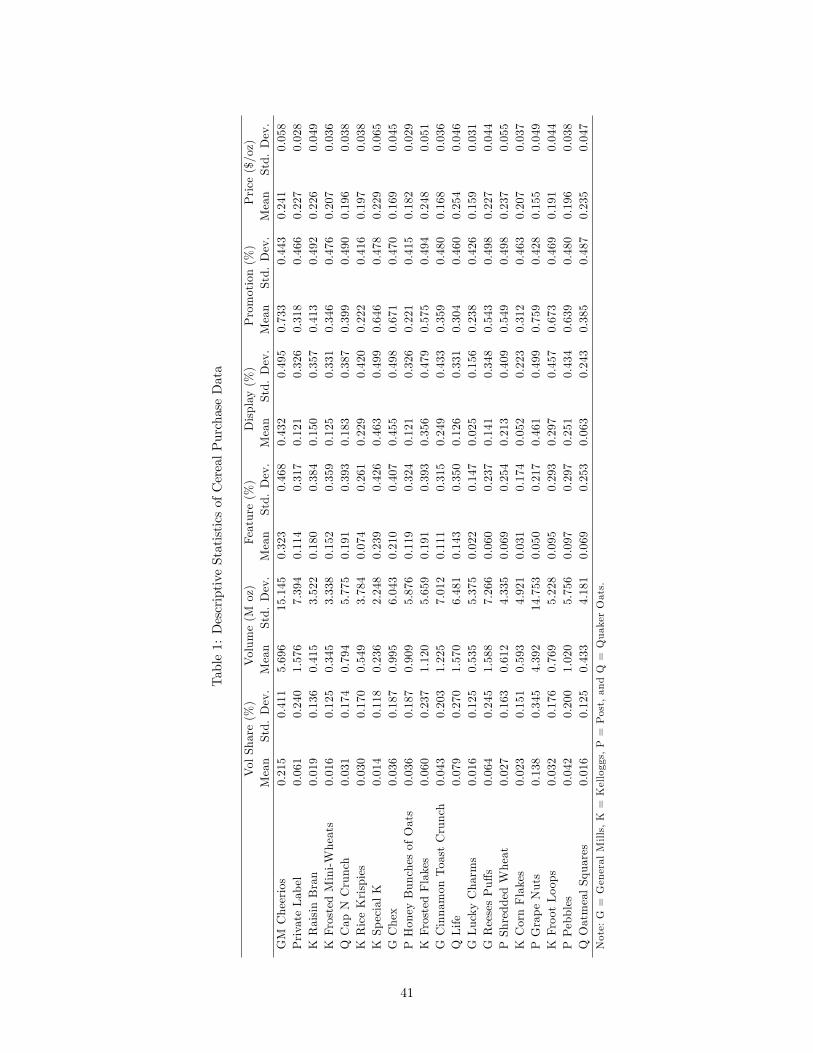
Table1:DescriptiveStatisticsofCerealPurchaseData

VolShare(%)

Volume(M

oz)

Feature(%)

Display(%)

Promotion(%)

Price($/oz)

Mean

Std.Dev.

Mean

Std.Dev.

Mean

Std.Dev.

Mean

Std.Dev.

Mean

Std.Dev.

Mean

Std.Dev.

GMCheerios

0.215

0.411

5.696

15.145

0.323

0.468

0.432

0.495

0.733

0.443

0.241

0.058

PrivateLabel

0.061

0.240

1.576

7.394

0.114

0.317

0.121

0.326

0.318

0.466

0.227

0.028

KRaisinBran

0.019

0.136

0.415

3.522

0.180

0.384

0.150

0.357

0.413

0.492

0.226

0.049

KFrostedMini-Wheats

0.016

0.125

0.345

3.338

0.152

0.359

0.125

0.331

0.346

0.476

0.207

0.036

QCapNCrunch

0.031

0.174

0.794

5.775

0.191

0.393

0.183

0.387

0.399

0.490

0.196

0.038

KRiceKrispies

0.030

0.170

0.549

3.784

0.074

0.261

0.229

0.420

0.222

0.416

0.197

0.038

KSpecialK

0.014

0.118

0.236

2.248

0.239

0.426

0.463

0.499

0.646

0.478

0.229

0.065

GChex

0.036

0.187

0.995

6.043

0.210

0.407

0.455

0.498

0.671

0.470

0.169

0.045

PHoneyBunchesofOats

0.036

0.187

0.909

5.876

0.119

0.324

0.121

0.326

0.221

0.415

0.182

0.029

KFrostedFlakes

0.060

0.237

1.120

5.659

0.191

0.393

0.356

0.479

0.575

0.494

0.248

0.051

GCinnamonToastCrunch

0.043

0.203

1.225

7.012

0.111

0.315

0.249

0.433

0.359

0.480

0.168

0.036

QLife

0.079

0.270

1.570

6.481

0.143

0.350

0.126

0.331

0.304

0.460

0.254

0.046

GLuckyCharms

0.016

0.125

0.535

5.375

0.022

0.147

0.025

0.156

0.238

0.426

0.159

0.031

GReesesPu¤s

0.064

0.245

1.588

7.266

0.060

0.237

0.141

0.348

0.543

0.498

0.227

0.044

PShreddedWheat

0.027

0.163

0.612

4.335

0.069

0.254

0.213

0.409

0.549

0.498

0.237

0.055

KCornFlakes

0.023

0.151

0.593

4.921

0.031

0.174

0.052

0.223

0.312

0.463

0.207

0.037

PGrapeNuts

0.138

0.345

4.392

14.753

0.050

0.217

0.461

0.499

0.759

0.428

0.155

0.049

KFrootLoops

0.032

0.176

0.769

5.228

0.095

0.293

0.297

0.457

0.673

0.469

0.191

0.044

PPebbles

0.042

0.200

1.020

5.756

0.097

0.297

0.251

0.434

0.639

0.480

0.196

0.038

QOatmealSquares

0.016

0.125

0.433

4.181

0.069

0.253

0.063

0.243

0.385

0.487

0.235

0.047

Note:G=GeneralMills,K=Kelloggs,P=Post,andQ=QuakerOats.

41

Table2:DescriptiveStatisticsofCerealShare,PriceandPromotionbyStore

Store1

Store2

VolShare(%)

Price($/oz)

Promotion(%)

VolShare(%)

Price($/oz)

Promotion(%)

Mean

Std.Dev.

Mean

Std.Dev.

Mean

Std.Dev.

Mean

Std.Dev.

Mean

Std.Dev.

Mean

Std.Dev.

GMCheerios

0.053

0.225

0.245

0.039

0.853

0.354

0.093

0.290

0.225

0.036

0.674

0.469

PrivateLabel

0.014

0.118

0.224

0.023

0.281

0.449

0.028

0.166

0.233

0.025

0.341

0.474

KRaisinBran

0.004

0.062

0.241

0.039

0.529

0.499

0.006

0.079

0.217

0.031

0.359

0.480

KFrostedMini-Wheats

0.005

0.069

0.215

0.032

0.579

0.494

0.004

0.061

0.198

0.026

0.223

0.416

QCapNCrunch

0.005

0.073

0.201

0.025

0.474

0.499

0.012

0.108

0.189

0.030

0.375

0.484

KRiceKrispies

0.007

0.083

0.218

0.029

0.418

0.493

0.015

0.120

0.171

0.011

0.109

0.312

KSpecialK

0.004

0.062

0.221

0.057

0.843

0.363

0.005

0.070

0.213

0.026

0.549

0.498

GChex

0.011

0.104

0.166

0.035

0.861

0.346

0.013

0.115

0.161

0.023

0.579

0.494

PHoneyBunchesofOats

0.011

0.106

0.195

0.024

0.502

0.500

0.011

0.105

0.169

0.005

0.073

0.260

KFrostedFlakes

0.017

0.131

0.248

0.039

0.859

0.348

0.025

0.157

0.224

0.021

0.436

0.496

GCinnamonToastCrunch

0.011

0.103

0.171

0.025

0.589

0.492

0.022

0.146

0.155

0.010

0.257

0.437

QLife

0.029

0.169

0.277

0.031

0.381

0.486

0.027

0.163

0.233

0.012

0.278

0.448

GLuckyCharms

0.004

0.060

0.155

0.015

0.157

0.364

0.006

0.078

0.149

0.015

0.290

0.454

GReesesPu¤s

0.015

0.121

0.238

0.036

0.395

0.489

0.029

0.167

0.221

0.032

0.656

0.475

PShreddedWheat

0.005

0.073

0.242

0.053

0.495

0.500

0.009

0.096

0.235

0.045

0.612

0.487

KCornFlakes

0.005

0.072

0.211

0.029

0.233

0.423

0.011

0.105

0.197

0.031

0.368

0.482

PGrapeNuts

0.046

0.211

0.148

0.029

0.782

0.413

0.059

0.237

0.147

0.031

0.758

0.428

KFrootLoops

0.008

0.087

0.208

0.046

0.655

0.475

0.015

0.120

0.180

0.026

0.691

0.462

PPebbles

0.009

0.096

0.206

0.040

0.580

0.494

0.017

0.130

0.188

0.026

0.700

0.458

QOatmealSquares

0.002

0.043

0.251

0.041

0.171

0.377

0.007

0.081

0.224

0.045

0.522

0.500

Note:G=GeneralMills,K=Kelloggs,P=Post,andQ=QuakerOats.

42

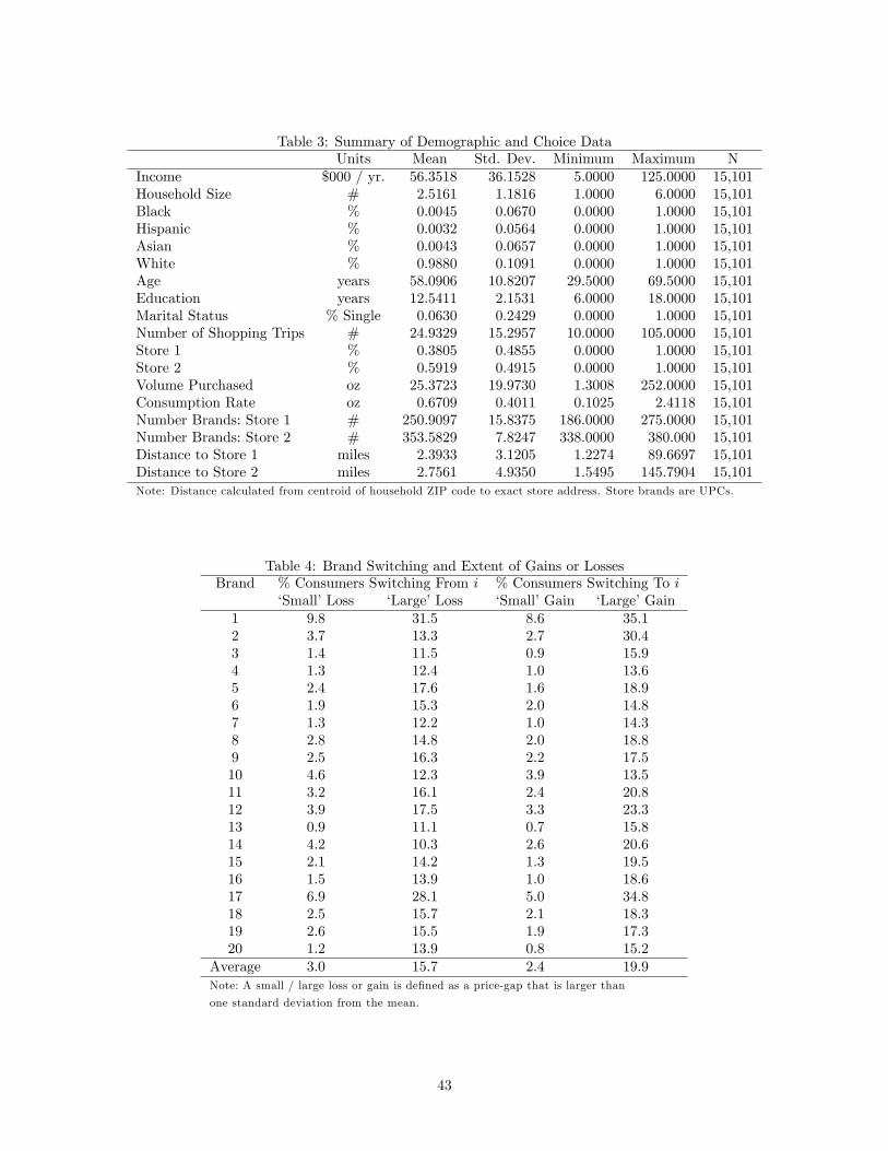
Table 3: Summary of Demographic and Choice DataUnits Mean Std. Dev. Minimum Maximum N

Income $000 / yr. 56.3518 36.1528 5.0000 125.0000 15,101Household Size # 2.5161 1.1816 1.0000 6.0000 15,101Black % 0.0045 0.0670 0.0000 1.0000 15,101Hispanic % 0.0032 0.0564 0.0000 1.0000 15,101Asian % 0.0043 0.0657 0.0000 1.0000 15,101White % 0.9880 0.1091 0.0000 1.0000 15,101Age years 58.0906 10.8207 29.5000 69.5000 15,101Education years 12.5411 2.1531 6.0000 18.0000 15,101Marital Status % Single 0.0630 0.2429 0.0000 1.0000 15,101Number of Shopping Trips # 24.9329 15.2957 10.0000 105.0000 15,101Store 1 % 0.3805 0.4855 0.0000 1.0000 15,101Store 2 % 0.5919 0.4915 0.0000 1.0000 15,101Volume Purchased oz 25.3723 19.9730 1.3008 252.0000 15,101Consumption Rate oz 0.6709 0.4011 0.1025 2.4118 15,101Number Brands: Store 1 # 250.9097 15.8375 186.0000 275.0000 15,101Number Brands: Store 2 # 353.5829 7.8247 338.0000 380.000 15,101Distance to Store 1 miles 2.3933 3.1205 1.2274 89.6697 15,101Distance to Store 2 miles 2.7561 4.9350 1.5495 145.7904 15,101Note: Distance calculated from centroid of household ZIP code to exact store address. Store brands are UPCs.

Table 4: Brand Switching and Extent of Gains or LossesBrand % Consumers Switching From i % Consumers Switching To i

�Small�Loss �Large�Loss �Small�Gain �Large�Gain1 9.8 31.5 8.6 35.12 3.7 13.3 2.7 30.43 1.4 11.5 0.9 15.94 1.3 12.4 1.0 13.65 2.4 17.6 1.6 18.96 1.9 15.3 2.0 14.87 1.3 12.2 1.0 14.38 2.8 14.8 2.0 18.89 2.5 16.3 2.2 17.510 4.6 12.3 3.9 13.511 3.2 16.1 2.4 20.812 3.9 17.5 3.3 23.313 0.9 11.1 0.7 15.814 4.2 10.3 2.6 20.615 2.1 14.2 1.3 19.516 1.5 13.9 1.0 18.617 6.9 28.1 5.0 34.818 2.5 15.7 2.1 18.319 2.6 15.5 1.9 17.320 1.2 13.9 0.8 15.2

Average 3.0 15.7 2.4 19.9Note: A small / large loss or gain is de�ned as a price-gap that is larger than

one standard deviation from the mean.

43

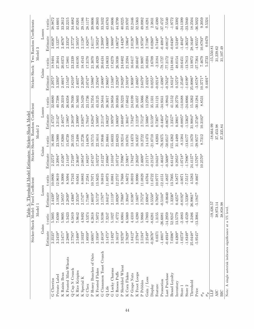
Table5:ThresholdModelEstimates:Sticker-ShockModel

Sticker-ShockModel:FixedCoe¢cient

Sticker-Shock:RandomCoe¢cient

Sticker-Shock:TwoRandomCoe¢cients

Model1

Model2

Model3

Gains

Losses

Gains

Losses

Gains

Losses

Estimate

t-ratio

Estimate

t-ratio

Estimate

t-ratio

Estimate

t-ratio

Estimate

t-ratio

Estimate

t-ratio

GCheerios

2.3535*

5.5605

2.4439*

10.0800

2.2273*

16.4080

2.4755*

32.6680

2.2975*

18.9404

2.6026*

38.9872

PrivateLabel

3.2459*

7.6500

3.1932*

12.9619

3.2094*

23.5900

3.2142*

40.7398

3.3393*

27.3044

3.1227*

44.6601

KRaisinBran

2.5471*

5.9695

2.5855*

9.3909

2.4526*

17.9260

2.4857*

29.3319

2.4601*

20.0373

2.4676*

33.2612

KFrostedMini-Wheats

2.2800*

5.3423

2.2839*

8.5094

2.1410*

15.6739

2.1985*

26.6358

2.1543*

17.5801

2.3352*

32.2215

QCapNCrunch

2.7785*

6.5819

2.4366*

9.7243

2.7249*

20.1535

2.3819*

30.7030

2.8210*

23.2339

2.3772*

34.4682

KRiceKrispies

2.5408*

5.9642

2.3534*

9.6561

2.3640*

17.3498

2.3999*

31.5603

2.4037*

19.6195

2.5055*

37.0201

KSpecialK

2.1033*

4.9492

2.1747*

8.0883

2.0854*

15.2726

2.0387*

24.5429

2.2659*

18.4543

2.1128*

29.1186

GChex

1.8959*

4.5374

1.7166*

7.2581

1.8825*

14.0878

1.7044*

23.1736

2.0747*

17.3170

1.8287*

28.1177

PHoneyBunchesofOats

2.6691*

6.2618

2.6019*

10.7071

2.6745*

19.5715

2.6284*

34.7354

2.5986*

21.3070

2.6117*

39.0606

KFrostedFlakes

3.1958*

7.5072

3.5173*

13.5625

3.0272*

22.1614

3.5095*

43.3125

3.2504*

26.4929

3.5024*

49.2603

GCinnamonToastCrunch

2.4818*

5.9198

2.1787*

9.0819

2.4122*

17.9946

2.2114*

29.5844

2.4800*

20.6434

2.2089*

33.3432

QLife

3.1475*

7.3247

3.0412*

11.8973

2.8986*

21.0664

3.0623*

38.3017

2.9665*

24.0633

3.0609*

43.6783

GLuckyCharms

2.1492*

5.1027

2.1119*

8.0981

2.1016*

15.6033

1.9979*

24.9858

2.1340*

17.6279

1.9880*

27.8606

GReesesPu¤s

3.1613*

7.4772

3.0928*

12.2757

3.0712*

22.6823

3.0693*

39.0383

3.2283*

26.5938

3.0672*

44.3799

PShreddedWheat

2.9270*

6.8904

2.7068*

9.7668

2.7096*

19.9214

2.6049*

30.5223

2.9420*

24.0402

3.4426*

40.0225

KCornFlakes

2.7629*

6.5069

1.3944*

5.8672

2.5901*

19.0781

1.3041*

17.6642

2.5919*

21.2594

1.5964*

23.9707

PGrapeNuts

1.8412*

4.4310

1.8198*

8.0919

1.7842*

13.4373

1.7342*

24.8199

1.9038*

16.0417

2.0126*

32.2446

KFrootLoops

2.2794*

5.4280

2.1607*

8.9990

2.2633*

16.8357

2.1219*

28.4357

2.4865*

20.6047

2.1609*

32.5363

PPebbles

2.5194*

5.9868

2.7572*

11.0829

2.4609*

18.2722

2.7512*

35.5066

2.6479*

21.9097

3.9750*

49.0982

Gain/Loss

2.2549*

4.7803

2.6984*

4.6764

2.2171*

14.1473

2.5066*

13.2700

2.4324*

16.0204

2.7106*

18.4281

Display

-0.2676*

-8.6281

0.5550*

11.6722

-0.2153*

-21.0710

0.5159*

35.1331

0.0255*

2.6709

0.0260*

2.3831

Feature

0.0371

1.3155

0.7682*

10.9777

0.0431*

4.6203

0.7307*

34.1121

-0.0214*

-2.3184

0.7448*

47.4380

Promotion

-1.4801*

-26.6081

-0.5104*

-12.4151

-1.4643*

-76.9375

-0.4464*

-34.9341

-1.4386*

-78.1727

-0.4084*

-37.4727

LastPurchase

-0.4934*

-14.2959

-0.0640

-1.4837

-0.5609*

-50.0517

-0.0673*

-4.9943

-0.7652*

-77.2172

-0.0812*

-7.5540

BrandLoyalty

7.0396*

52.9247

1.3236*

13.7005

6.6142*

155.4262

1.2357*

41.5152

3.8312*

124.0841

-0.0438*

-1.9772

Inventory

0.4269*

13.5779

0.4257*

8.5877

0.2955*

31.4489

0.3901*

26.2770

0.5273*

48.0154

0.5249*

40.3392

Store1

-1.0273*

-2.4883

-0.8192*

-4.0071

-1.0718*

-8.1384

-0.8885*

-14.0488

-1.2540*

-10.6451

-1.4042*

-24.1399

Store2

-1.8349*

-4.4529

-1.5230*

-7.5517

-1.7896*

-13.6177

-1.5363*

-24.6066

-1.6199*

-13.7813

-1.3653*

-23.5940

Threshold

25.0448*

4.2486

26.9961*

4.5283

24.4137*

11.1670

31.9084*

15.3262

25.0086*

12.9972

28.1640*

18.2504

Price

-5.9545*

-13.3064

-5.1947*

-9.4667

-4.5797*

-29.9577

-5.2748*

-30.1284

-3.8578*

-27.7264

-4.9555*

-36.5022

�g

10.2570*

8.7312

10.3102*

8.8531

10.3771*

7.4679

10.8793*

9.2059

�p

0.4401*

5.2733

0.0470

0.5324

LLF

-19,426.57

-18,664.99

-15,550.81

AIC

38,973.14

37,453.98

31,229.62

BIC

38,858.98

37,335.84

31,107.49

Note:Asingleasteriskindicatessigni�canceata5%

level.

44

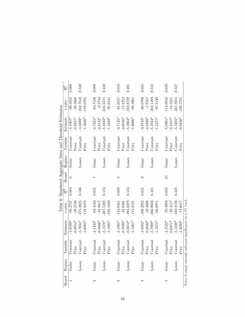
Table6:SimulatedAggregateDataandThresholdEstimates

Brand

Regime

Variable

Estimate

t-ratio

R2

Brand

Regime

Variable

Estimate

t-ratio

R2

1Gains

Constant

-5.0189*

-98.2757

0.064

6Gains

Constant

-4.1967*

-96.1652

0.069

Price

-0.9754*

-28.2146

Price

-0.8957*

-29.3968

Losses

Constant

-5.7034*

-275.2625

0.546

Losses

Constant

-4.6809*

-242.7848

0.538

Price

-1.6562*

-118.0478

Price

-1.5636*

-116.0765

2Gains

Constant

-4.1433*

-83.4163

0.031

7Gains

Constant

-3.7355*

-63.7126

0.009

Price

-0.5698*

-18.9917

Price

-0.3142*

-9.7754

Losses

Constant

-5.1578*

-267.5202

0.574

Losses

Constant

-5.4833*

-245.5571

0.438

Price

-1.1895*

-102.1039

Price

-1.1633*

-95.0441

3Gains

Constant

-5.1985*

-144.0421

0.089

8Gains

Constant

-3.7135*

-61.6557

0.019

Price

-0.7880*

-33.6591

Price

-0.6556*

-15.2312

Losses

Constant

-6.0012*

-293.0278

0.534

Losses

Constant

-5.2063*

-222.8729

0.461

Price

-1.5301*

-115.2191

Price

-1.6606*

-99.4961

4Gains

Constant

-4.8832*

-106.2952

0.031

9Gains

Constant

-3.8710*

-66.0700

0.045

Price

-0.4833*

-19.3308

Price

-0.2499*

-7.9767

Losses

Constant

-5.7989*

-266.8633

0.431

Losses

Constant

-5.7044*

-262.1489

0.552

Price

-1.1075*

-93.6971

Price

-1.1377*

-97.7440

5Gains

Constant

-4.1522*

-70.4959

0.035

10Gains

Constant

-5.0361*

-114.0942

0.049

Price

-0.6971*

-20.4117

Price

-0.5557*

-24.5221

Losses

Constant

-5.1220*

-180.4146

0.325

Losses

Constant

-5.5205*

-361.7654

0.557

Price

-1.2293*

-74.6817

Price

-0.9456*

-120.7701

Note:Asingleasteriskindicatessigni�canceata5%

level.

45

Table7:AlternateThresholdModelEstimates:Cereal

ThresholdModel:NoVolatilityTerm

ThresholdModel:Volatility,FixedCoe¢cient

ThresholdModel:RandomCoe¢cient

Model4

Model5

Model6

Gains

Losses

Gains

Losses

Gains

Losses

Estimate

t-ratio

Estimate

t-ratio

Estimate

t-ratio

Estimate

t-ratio

Estimate

t-ratio

Estimate

t-ratio

GCheerios

2.2649*

3.6670

2.3134*

6.3228

2.4619*

4.1128

2.3168*

7.5019

2.4948*

17.8378

2.5427*

24.9681

PrivateLabel

3.1933*

5.1468

3.2786*

8.4853

3.3186*

5.5267

2.4869*

7.8843

3.1795*

22.5869

2.8252*

27.2638

KRaisinBran

2.1352*

3.4399

2.6426*

6.5776

2.5470*

4.2264

2.6006*

7.2304

3.2055*

22.1586

2.5170*

22.4392

KFrostedMini-Wheats

2.2396*

3.5890

2.3441*

5.8847

2.3425*

3.8807

2.2706*

6.5703

2.4952*

17.4473

2.2203*

20.4550

QCapNCrunch

2.7025*

4.3589

2.4903*

6.5216

2.9906*

4.9814

2.2163*

6.9980

2.9891*

21.1491

2.2373*

21.3440

KRiceKrispies

2.4761*

3.9679

2.4173*

6.3757

2.6046*

4.3127

2.1162*

6.6614

2.7732*

19.3432

2.5721*

24.4230

KSpecialK

1.9242*

3.0993

1.9505*

5.0297

2.2839*

3.7859

2.1219*

6.0575

2.8272*

19.5670

2.0564*

18.3736

GChex

1.7717*

2.8667

1.6755*

4.5149

2.0966*

3.4998

1.7107*

5.4229

2.1807*

15.5438

2.7346*

25.5076

PHoneyBunchesofOats

2.6307*

4.1953

2.6794*

7.0829

2.6462*

4.3728

2.3198*

7.3259

2.8445*

19.8744

2.8767*

27.3201

KFrostedFlakes

3.1238*

5.0396

3.5302*

9.4992

3.2228*

5.3603

8.3774*

5.2581

3.1333*

22.2112

3.0210*

28.7811

GCinnamonToastCrunch

2.3862*

3.8552

2.2396*

5.9610

2.6288*

4.3835

1.8052*

5.7462

2.5676*

18.2781

2.4423*

23.2748

QLife

3.1172*

4.9800

3.0294*

8.0981

2.9296*

4.8613

2.7863*

8.8672

3.0317*

21.3929

2.4594*

24.0979

GLuckyCharms

1.9962*

3.2175

2.0107*

5.1368

2.2688*

3.7732

2.2362*

6.4248

2.9262*

20.2230

2.1297*

19.3670

GReesesPu¤s

3.0643*

4.9439

3.0873*

8.1339

3.0237*

5.0435

2.6753*

8.3883

3.0423*

21.6511

2.9558*

28.1517

PShreddedWheat

2.8167*

4.5322

2.7716*

6.8872

2.7907*

4.6407

2.7492*

7.5991

3.0845*

21.7252

2.6813*

23.7772

KCornFlakes

2.6027*

4.1855

2.6675*

6.8473

2.8768*

4.7718

1.3845*

4.4183

3.4736*

23.9212

1.6025*

15.5184

PGrapeNuts

1.9123*

3.0972

1.7449*

4.7624

1.9086*

3.1912

1.5730*

5.1122

2.1436*

15.3252

1.8414*

18.0834

KFrootLoops

2.1357*

3.4531

2.2163*

5.9381

2.5212*

4.2051

1.9731*

6.2382

2.9990*

21.2035

2.4915*

23.5431

PPebbles

2.4211*

3.9127

2.8229*

7.4314

2.6437*

4.4109

2.3412*

7.3666

2.6714*

19.0094

2.6157*

24.9245

Gain/Loss

2.3612*

5.7627

2.7202*

5.6985

2.2872*

5.7228

3.1815*

5.9074

1.9224*

14.3752

1.9070*

11.4103

Display

-0.3802*

-9.6378

0.4663*

10.4118

-0.3962*

-10.7609

0.5083*

10.8924

-0.3404*

-28.3118

0.5681*

40.5645

Feature

-0.0860*

-2.6131

0.7644*

12.4971

-0.1360*

-4.5675

0.4097*

7.6110

-0.0759*

-7.5101

0.3536*

19.7287

Promotion

-1.5750*

-19.4597

-1.2390*

-23.7560

-1.6203*

-20.0124

-0.7765*

-16.8312

-1.6736*

-60.0443

-0.7573*

-55.2694

LastPurchase

-0.5781*

-14.1459

-0.2253*

-5.0558

-0.5283*

-14.6165

-0.2774*

-6.3643

-0.5479*

-48.2602

-0.2903*

-21.9420

BrandLoyalty

7.2531*

44.0095

1.2314*

12.4150

5.3354*

42.1988

0.4872*

5.2900

2.3453*

76.3474

0.0944*

3.4940

Inventory

0.4219*

11.5509

0.2897*

6.1436

0.4115*

12.3455

0.3425*

7.2954

0.3026*

28.8700

0.4291*

29.2250

Store1

-1.2211*

-1.9681

-1.4598*

-3.9931

-1.2530*

-2.0838

-1.4437*

-4.7361

-1.1056*

-7.8169

-2.0275*

-20.1501

Store2

-1.9311*

-3.1162

-1.7826*

-4.8934

-1.9690*

-3.2789

-1.7503*

-5.7710

-1.1758*

-8.3272

-1.8364*

-18.2891

Threshold

25.2902*

3.0295

27.2581*

3.0206

29.5879*

12.5708

32.2448*

13.2679

�g

11.5540*

9.2482

11.4671*

7.7844

LLF

-21,504.78

-19,645.17

-15,804.01

AIC

43,117.56

39,402.34

-31,492.02

BIC

43,015.36

39,296.15

-31,602.19

Note:Asingleasteriskindicatessigni�canceata5%

level.

46

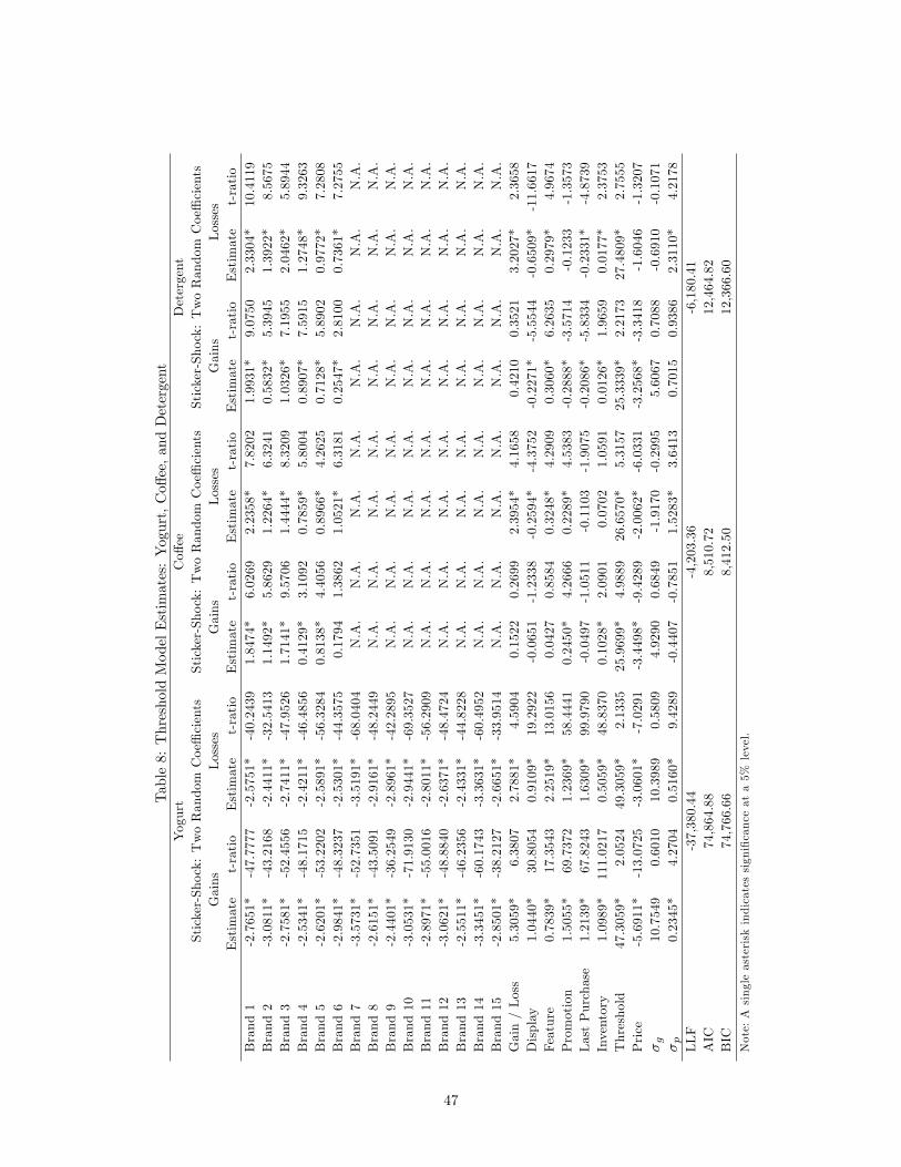
Table8:ThresholdModelEstimates:Yogurt,Co¤ee,andDetergent

Yogurt

Co¤ee

Detergent

Sticker-Shock:TwoRandomCoe¢cients

Sticker-Shock:TwoRandomCoe¢cients

Sticker-Shock:TwoRandomCoe¢cients

Gains

Losses

Gains

Losses

Gains

Losses

Estimate

t-ratio

Estimate

t-ratio

Estimate

t-ratio

Estimate

t-ratio

Estimate

t-ratio

Estimate

t-ratio

Brand1

-2.7651*

-47.7777

-2.5751*

-40.2439

1.8474*

6.0269

2.2358*

7.8202

1.9931*

9.0750

2.3304*

10.4119

Brand2

-3.0811*

-43.2168

-2.4411*

-32.5413

1.1492*

5.8629

1.2264*

6.3241

0.5832*

5.3945

1.3922*

8.5675

Brand3

-2.7581*

-52.4556

-2.7411*

-47.9526

1.7141*

9.5706

1.4444*

8.3209

1.0326*

7.1955

2.0462*

5.8944

Brand4

-2.5341*

-48.1715

-2.4211*

-46.4856

0.4129*

3.1092

0.7859*

5.8004

0.8907*

7.5915

1.2748*

9.3263

Brand5

-2.6201*

-53.2202

-2.5891*

-56.3284

0.8138*

4.4056

0.8966*

4.2625

0.7128*

5.8902

0.9772*

7.2808

Brand6

-2.9841*

-48.3237

-2.5301*

-44.3575

0.1794

1.3862

1.0521*

6.3181

0.2547*

2.8100

0.7361*

7.2755

Brand7

-3.5731*

-52.7351

-3.5191*

-68.0404

N.A.

N.A.

N.A.

N.A.

N.A.

N.A.

N.A.

N.A.

Brand8

-2.6151*

-43.5091

-2.9161*

-48.2449

N.A.

N.A.

N.A.

N.A.

N.A.

N.A.

N.A.

N.A.

Brand9

-2.4401*

-36.2549

-2.8961*

-42.2895

N.A.

N.A.

N.A.

N.A.

N.A.

N.A.

N.A.

N.A.

Brand10

-3.0531*

-71.9130

-2.9441*

-69.3527

N.A.

N.A.

N.A.

N.A.

N.A.

N.A.

N.A.

N.A.

Brand11

-2.8971*

-55.0016

-2.8011*

-56.2909

N.A.

N.A.

N.A.

N.A.

N.A.

N.A.

N.A.

N.A.

Brand12

-3.0621*

-48.8840

-2.6371*

-48.4724

N.A.

N.A.

N.A.

N.A.

N.A.

N.A.

N.A.

N.A.

Brand13

-2.5511*

-46.2356

-2.4331*

-44.8228

N.A.

N.A.

N.A.

N.A.

N.A.

N.A.

N.A.

N.A.

Brand14

-3.3451*

-60.1743

-3.3631*

-60.4952

N.A.

N.A.

N.A.

N.A.

N.A.

N.A.

N.A.

N.A.

Brand15

-2.8501*

-38.2127

-2.6651*

-33.9514

N.A.

N.A.

N.A.

N.A.

N.A.

N.A.

N.A.

N.A.

Gain/Loss

5.3059*

6.3807

2.7881*

4.5904

0.1522

0.2699

2.3954*

4.1658

0.4210

0.3521

3.2027*

2.3658

Display

1.0440*

30.8054

0.9109*

19.2922

-0.0651

-1.2338

-0.2594*

-4.3752

-0.2271*

-5.5544

-0.6509*

-11.6617

Feature

0.7839*

17.3543

2.2519*

13.0156

0.0427

0.8584

0.3248*

4.2909

0.3060*

6.2635

0.2979*

4.9674

Promotion

1.5055*

69.7372

1.2369*

58.4441

0.2450*

4.2666

0.2289*

4.5383

-0.2888*

-3.5714

-0.1233

-1.3573

LastPurchase

1.2139*

67.8243

1.6309*

99.9790

-0.0497

-1.0511

-0.1103

-1.9075

-0.2086*

-5.8334

-0.2331*

-4.8739

Inventory

1.0989*

111.0217

0.5059*

48.8370

0.1028*

2.0901

0.0702

1.0591

0.0126*

1.9659

0.0177*

2.3753

Threshold

47.3059*

2.0524

49.3059*

2.1335

25.9699*

4.9889

26.6570*

5.3157

25.3339*

2.2173

27.4809*

2.7555

Price

-5.6911*

-13.0725

-3.0601*

-7.0291

-3.4498*

-9.4289

-2.0062*

-6.0331

-3.2568*

-3.3418

-1.6046

-1.3207

�g

10.7549

0.6010

10.3989

0.5809

4.9290

0.6849

-1.9170

-0.2995

5.6067

0.7088

-0.6910

-0.1071

�p

0.2345*

4.2704

0.5160*

9.4289

-0.4407

-0.7851

1.5283*

3.6413

0.7015

0.9386

2.3110*

4.2178

LLF

-37,380.44

-4,203.36

-6,180.41

AIC

74,864.88

8,510.72

12,464.82

BIC

74,766.66

8,412.50

12,366.60

Note:Asingleasteriskindicatessigni�canceata5%

level.

47