Hypre-2.0.0 Usr Manual
83
User’s Manual Software Version: 2.0.0 Date: 2006/12/15 Center for Applied Scientific Computing Lawrence Livermore National Laboratory
Transcript of Hypre-2.0.0 Usr Manual
User’s Manual
Software Version: 2.0.0Date: 2006/12/15
Center for Applied Scientific ComputingLawrence Livermore National Laboratory

Copyright (c) 2006 The Regents of the University of California. Produced at the Lawrence Liv-ermore National Laboratory. Written by the HYPRE team. UCRL-CODE-222953. All rightsreserved.
This file is part of HYPRE (see http://www.llnl.gov/CASC/hypre/). Please see the COPY-RIGHT and LICENSE file for the copyright notice, disclaimer, contact information and the GNULesser General Public License.
HYPRE is free software; you can redistribute it and/or modify it under the terms of the GNUGeneral Public License (as published by the Free Software Foundation) version 2.1 dated February1999.
HYPRE is distributed in the hope that it will be useful, but WITHOUT ANY WARRANTY;without even the IMPLIED WARRANTY OF MERCHANTABILITY or FITNESS FOR A PAR-TICULAR PURPOSE. See the terms and conditions of the GNU General Public License for moredetails.
You should have received a copy of the GNU Lesser General Public License along with this program;if not, write to the Free Software Foundation, Inc., 59 Temple Place, Suite 330, Boston, MA 02111-1307 USA

Contents
1 Introduction 11.1 Overview of Features . . . . . . . . . . . . . . . . . . . . . . . . . . . . . . . . . . . . 11.2 Getting More Information . . . . . . . . . . . . . . . . . . . . . . . . . . . . . . . . . 21.3 How to get started . . . . . . . . . . . . . . . . . . . . . . . . . . . . . . . . . . . . . 3
1.3.1 Installing hypre . . . . . . . . . . . . . . . . . . . . . . . . . . . . . . . . . . . 31.3.2 Choosing a conceptual interface . . . . . . . . . . . . . . . . . . . . . . . . . . 31.3.3 Writing your code . . . . . . . . . . . . . . . . . . . . . . . . . . . . . . . . . 5
2 Structured-Grid System Interface (Struct) 72.1 Setting Up the Struct Grid . . . . . . . . . . . . . . . . . . . . . . . . . . . . . . . . 82.2 Setting Up the Struct Stencil . . . . . . . . . . . . . . . . . . . . . . . . . . . . . . . 102.3 Setting Up the Struct Matrix . . . . . . . . . . . . . . . . . . . . . . . . . . . . . . . 102.4 Setting Up the Struct Right-Hand-Side Vector . . . . . . . . . . . . . . . . . . . . . 132.5 Symmetric Matrices . . . . . . . . . . . . . . . . . . . . . . . . . . . . . . . . . . . . 14
3 Semi-Structured-Grid System Interface (SStruct) 173.1 Block-Structured Grids . . . . . . . . . . . . . . . . . . . . . . . . . . . . . . . . . . 183.2 Structured Adaptive Mesh Refinement . . . . . . . . . . . . . . . . . . . . . . . . . . 22
4 Finite Element Interface 274.1 Introduction . . . . . . . . . . . . . . . . . . . . . . . . . . . . . . . . . . . . . . . . . 274.2 A Brief Description of the Finite Element Interface . . . . . . . . . . . . . . . . . . . 28
5 Linear-Algebraic System Interface (IJ) 315.1 IJ Matrix Interface . . . . . . . . . . . . . . . . . . . . . . . . . . . . . . . . . . . . . 315.2 IJ Vector Interface . . . . . . . . . . . . . . . . . . . . . . . . . . . . . . . . . . . . . 335.3 A Scalable Interface . . . . . . . . . . . . . . . . . . . . . . . . . . . . . . . . . . . . 34
6 Solvers and Preconditioners 356.1 SMG . . . . . . . . . . . . . . . . . . . . . . . . . . . . . . . . . . . . . . . . . . . . . 376.2 PFMG . . . . . . . . . . . . . . . . . . . . . . . . . . . . . . . . . . . . . . . . . . . . 386.3 SysPFMG . . . . . . . . . . . . . . . . . . . . . . . . . . . . . . . . . . . . . . . . . . 386.4 SplitSolve . . . . . . . . . . . . . . . . . . . . . . . . . . . . . . . . . . . . . . . . . . 38
i

ii CONTENTS
6.5 FAC . . . . . . . . . . . . . . . . . . . . . . . . . . . . . . . . . . . . . . . . . . . . . 386.6 Maxwell . . . . . . . . . . . . . . . . . . . . . . . . . . . . . . . . . . . . . . . . . . . 396.7 Hybrid . . . . . . . . . . . . . . . . . . . . . . . . . . . . . . . . . . . . . . . . . . . . 416.8 BoomerAMG . . . . . . . . . . . . . . . . . . . . . . . . . . . . . . . . . . . . . . . . 41
6.8.1 Parameter Options . . . . . . . . . . . . . . . . . . . . . . . . . . . . . . . . . 416.9 AMS . . . . . . . . . . . . . . . . . . . . . . . . . . . . . . . . . . . . . . . . . . . . . 43
6.9.1 Overview . . . . . . . . . . . . . . . . . . . . . . . . . . . . . . . . . . . . . . 436.9.2 Sample Usage . . . . . . . . . . . . . . . . . . . . . . . . . . . . . . . . . . . . 44
6.10 The MLI Package . . . . . . . . . . . . . . . . . . . . . . . . . . . . . . . . . . . . . . 476.11 ParaSails . . . . . . . . . . . . . . . . . . . . . . . . . . . . . . . . . . . . . . . . . . 48
6.11.1 Parameter Settings . . . . . . . . . . . . . . . . . . . . . . . . . . . . . . . . . 486.11.2 Preconditioning Nearly Symmetric Matrices . . . . . . . . . . . . . . . . . . . 49
6.12 Euclid . . . . . . . . . . . . . . . . . . . . . . . . . . . . . . . . . . . . . . . . . . . . 496.12.1 Overview . . . . . . . . . . . . . . . . . . . . . . . . . . . . . . . . . . . . . . 506.12.2 Setting Options: Examples . . . . . . . . . . . . . . . . . . . . . . . . . . . . 516.12.3 Options Summary . . . . . . . . . . . . . . . . . . . . . . . . . . . . . . . . . 52
6.13 PILUT: Parallel Incomplete Factorization . . . . . . . . . . . . . . . . . . . . . . . . 536.14 FEI Solvers . . . . . . . . . . . . . . . . . . . . . . . . . . . . . . . . . . . . . . . . . 54
6.14.1 Solvers Available Only through the FEI . . . . . . . . . . . . . . . . . . . . . 54
7 General Information 577.1 Getting the Source Code . . . . . . . . . . . . . . . . . . . . . . . . . . . . . . . . . . 577.2 Building the Library . . . . . . . . . . . . . . . . . . . . . . . . . . . . . . . . . . . . 57
7.2.1 Configure Options . . . . . . . . . . . . . . . . . . . . . . . . . . . . . . . . . 587.2.2 Make Targets . . . . . . . . . . . . . . . . . . . . . . . . . . . . . . . . . . . . 59
7.3 Testing the Library . . . . . . . . . . . . . . . . . . . . . . . . . . . . . . . . . . . . . 597.4 Linking to the Library . . . . . . . . . . . . . . . . . . . . . . . . . . . . . . . . . . . 607.5 Error Flags . . . . . . . . . . . . . . . . . . . . . . . . . . . . . . . . . . . . . . . . . 607.6 Bug Reporting and General Support . . . . . . . . . . . . . . . . . . . . . . . . . . . 617.7 Using HYPRE in External FEI Implementations . . . . . . . . . . . . . . . . . . . . 617.8 Calling HYPRE from Other Languages . . . . . . . . . . . . . . . . . . . . . . . . . 62
8 Babel-based Interfaces 658.1 Introduction . . . . . . . . . . . . . . . . . . . . . . . . . . . . . . . . . . . . . . . . . 658.2 Interfaces Are Similar . . . . . . . . . . . . . . . . . . . . . . . . . . . . . . . . . . . 658.3 Interfaces Are Different . . . . . . . . . . . . . . . . . . . . . . . . . . . . . . . . . . 668.4 Names and Conventions . . . . . . . . . . . . . . . . . . . . . . . . . . . . . . . . . . 668.5 Parameters and Error Flags . . . . . . . . . . . . . . . . . . . . . . . . . . . . . . . . 678.6 MPI Communicator . . . . . . . . . . . . . . . . . . . . . . . . . . . . . . . . . . . . 688.7 Memory Management . . . . . . . . . . . . . . . . . . . . . . . . . . . . . . . . . . . 698.8 Casting . . . . . . . . . . . . . . . . . . . . . . . . . . . . . . . . . . . . . . . . . . . 708.9 The HYPRE Object Structure . . . . . . . . . . . . . . . . . . . . . . . . . . . . . . 718.10 Arrays . . . . . . . . . . . . . . . . . . . . . . . . . . . . . . . . . . . . . . . . . . . . 72

CONTENTS iii
8.11 Building HYPRE with the Babel Interface . . . . . . . . . . . . . . . . . . . . . . . . 738.11.1 Building HYPRE with Python Using the Babel Interface . . . . . . . . . . . 74

iv CONTENTS

Chapter 1
Introduction
This manual describes hypre, a software library of high performance preconditioners and solvers forthe solution of large, sparse linear systems of equations on massively parallel computers. The hyprelibrary was created with the primary goal of providing users with advanced parallel preconditioners.The library features parallel multigrid solvers for both structured and unstructured grid problems.For ease of use, these solvers are accessed from the application code via hypre’s conceptual linearsystem interfaces (abbreviated to conceptual interfaces throughout much of this manual), whichallow a variety of natural problem descriptions.
This introductory chapter provides an overview of the various features in hypre, discusses furthersources of information on hypre, and offers suggestions on how to get started.
1.1 Overview of Features
• Scalable preconditioners provide efficient solution on today’s and tomorrow’s sys-tems: hypre contains several families of preconditioner algorithms focused on the scalablesolution of very large sparse linear systems. (Note that small linear systems, systems that aresolvable on a sequential computer, and dense systems are all better addressed by other librariesthat are designed specifically for them.) hypre includes “grey-box” algorithms that use morethan just the matrix to solve certain classes of problems more efficiently than general-purposelibraries. This includes algorithms such as structured multigrid.
• Suite of common iterative methods provides options for a spectrum of problems:hypre provides several of the most commonly used Krylov-based iterative methods to be usedin conjunction with its scalable preconditioners. This includes methods for nonsymmetricsystems such as GMRES and methods for symmetric matrices such as Conjugate Gradient.
• Intuitive grid-centric interfaces obviate need for complicated data structures andprovide access to advanced solvers: hypre has made a major step forward in usabilityfrom earlier generations of sparse linear solver libraries in that users do not have to learncomplicated sparse matrix data structures. Instead, hypre does the work of building thesedata structures for the user through a variety of conceptual interfaces, each appropriate to
1

2 CHAPTER 1. INTRODUCTION
different classes of users. These include stencil-based structured/semi-structured interfacesmost appropriate for finite-difference applications; a finite-element based unstructured inter-face; and a linear-algebra based interface. Each conceptual interface provides access to severalsolvers without the need to write new interface code.
• User options accommodate beginners through experts: hypre allows a spectrum ofexpertise to be applied by users. The beginning user can get up and running with a minimalamount of effort. More expert users can take further control of the solution process throughvarious parameters.
• Configuration options to suit your computing system: hypre allows a simple andflexible installation on a wide variety of computing systems. Users can tailor the installationto match their computing system. Options include debug and optimized modes, the abilityto change required libraries such as MPI and BLAS, a sequential mode, and modes enablingthreads for certain solvers. On most systems, however, hypre can be built by simply typingconfigure followed by make.
• Interfaces in multiple languages provide greater flexibility for applications: hypreis written in C (with the exception of the FEI interface, which is written in C++) and utilizesBabel to provide interfaces for users of Fortran 77, Fortran 90, C++, Python, and Java. Formore information on Babel, see http://www.llnl.gov/CASC/components/babel.html.
1.2 Getting More Information
This user’s manual consists of chapters describing each conceptual interface, a chapter detailingthe various linear solver options available, and detailed installation information. In addition to thismanual, a number of other information sources for hypre are available.
• Reference Manual: The reference manual comprehensively lists all of the interface andsolver functions available in hypre. The reference manual is ideal for determining the variousoptions available for a particular solver or for viewing the functions provided to describe aproblem for a particular interface.
• Example Problems: A suite of example problems is provided with the hypre installation.These examples reside in the examples subdirectory and demonstrate various features of thehypre library. Associated documentation may be accessed by viewing the README.html filein that same directory.
• Papers, Presentations, etc.: Articles and presentations related to the hypre softwarelibrary and the solvers available in the library are available from the hypre web page athttp://www.llnl.gov/CASC/hypre/.
• Mailing Lists: There are two hypre mailing lists that can be subscribed to through thehypre web page at http://www.llnl.gov/CASC/hypre/:
1.3. HOW TO GET STARTED 3
1. hypre-announce ([email protected]): The development team uses thislist to announce new general releases of hypre. It cannot be posted to by users.
2. hypre-beta-announce ([email protected]): The development teamuses this list to announce new beta releases of hypre. It cannot be posted to by users.
1.3 How to get started
1.3.1 Installing hypre
As previously noted, on most systems hypre can be built by simply typing configure followedby make in the top-level source directory. For more detailed instructions read the INSTALL fileprovided with the hypre distribution or refer to the last chapter in this manual. Note the followingrequirements:
• To run in parallel, hypre requires an installation of MPI.
• Configuration of hypre with threads requires an implementation of OpenMP. Currently, onlya subset of hypre is threaded.
• The hypre library currently does not support complex-valued systems.
1.3.2 Choosing a conceptual interface
An important decision to make before writing any code is to choose an appropriate conceptualinterface. These conceptual interfaces are intended to represent the way that applications developersnaturally think of their linear problem and to provide natural interfaces for them to pass thedata that defines their linear system into hypre. Essentially, these conceptual interfaces can beconsidered convenient utilities for helping a user build a matrix data structure for hypre solversand preconditioners. The top row of Figure 1.1 illustrates a number of conceptual interfaces.Generally, the conceptual interfaces are denoted by different types of computational grids, butother application features might also be used, such as geometrical information. For example,applications that use structured grids (such as in the left-most interface in the Figure 1.1) typicallyview their linear problems in terms of stencils and grids. On the other hand, applications that useunstructured grids and finite elements typically view their linear problems in terms of elements andelement stiffness matrices. Finally, the right-most interface is the standard linear-algebraic (matrixrows/columns) way of viewing the linear problem.
The hypre library currently supports four conceptual interfaces, and typically the appropriatechoice for a given problem is fairly obvious, e.g. a structured-grid interface is clearly inappropriatefor an unstructured-grid application.
• Structured-Grid System Interface (Struct): This interface is appropriate for applica-tions whose grids consist of unions of logically rectangular grids with a fixed stencil patternof nonzeros at each grid point. This interface supports only a single unknown per grid point.See Chapter 2 for details.

4 CHAPTER 1. INTRODUCTION
Data Layout
structured composite block-struc unstruc CSR
Linear Solvers
GMG, ... FAC, ... Hybrid, ... AMGe, ... ILU, ...
Linear System Interfaces
Figure 1.1: Graphic illustrating the notion of conceptual interfaces.
• Semi-Structured-Grid System Interface (SStruct): This interface is appropriate forapplications whose grids are mostly structured, but with some unstructured features. Exam-ples include block-structured grids, composite grids in structured adaptive mesh refinement(AMR) applications, and overset grids. This interface supports multiple unknowns per cell.See Chapter 3 for details.
• Finite Element Interface (FEI): This is appropriate for users who form their linear sys-tems from a finite element discretization. The interface mirrors typical finite element datastructures, including element stiffness matrices. Though this interface is provided in hypre,its definition was determined elsewhere (please email to Alan Williams [email protected] more information). See Chapter 4 for details.
• Linear-Algebraic System Interface (IJ): This is the traditional linear-algebraic inter-face. It can be used as a last resort by users for whom the other grid-based interfaces arenot appropriate. It requires more work on the user’s part, though still less than building par-allel sparse data structures. General solvers and preconditioners are available through thisinterface, but not specialized solvers which need more information. Our experience is thatusers with legacy codes, in which they already have code for building matrices in particularformats, find the IJ interface relatively easy to use. See Chapter 5 for details.
Generally, a user should choose the most specific interface that matches their application, be-cause this will allow them to use specialized and more efficient solvers and preconditioners withoutlosing access to more general solvers. For example, the second row of Figure 1.1 is a set of linearsolver algorithms. Each linear solver group requires different information from the user through theconceptual interfaces. So, the geometric multigrid algorithm (GMG) listed in the left-most box,

1.3. HOW TO GET STARTED 5
for example, can only be used with the left-most conceptual interface. On the other hand, the ILUalgorithm in the right-most box may be used with any conceptual interface. Matrix requirementsfor each solver and preconditioner are provided in Chapter 6 and in the hypre Reference Manual.Your desired solver strategy may influence your choice of conceptual interface. A typical user willselect a single Krylov method and a single preconditioner to solve their system.
The third row of Figure 1.1 is a list of data layouts or matrix/vector storage schemes. Therelationship between linear solver and storage scheme is similar to that of the conceptual interfaceand linear solver. Note that some of the interfaces in hypre currently only support one matrix/vectorstorage scheme choice. The conceptual interface, the desired solvers and preconditioners, and thematrix storage class must all be compatible.
1.3.3 Writing your code
As discussed in the previous section, the following decisions should be made before writing anycode:
1. Choose a conceptual interface.
2. Choose your desired solver strategy.
3. Look up matrix requirements for each solver and preconditioner.
4. Choose a matrix storage class that is compatible with your solvers and preconditioners andyour conceptual interface.
Once the previous decisions have been made, it is time to code your application to call hypre.At this point, reviewing the previously mentioned example codes provided with the hypre librarymay prove very helpful. The example codes demonstrate the following general structure of theapplication calls to hypre:
1. Build any necessary auxiliary structures for your chosen conceptual interface. Thisincludes, e.g., the grid and stencil structures if you are using the structured-grid interface.
2. Build the matrix, solution vector, and right-hand-side vector through your chosenconceptual interface. Each conceptual interface provides a series of calls for enteringinformation about your problem into hypre.
3. Build solvers and preconditioners and set solver parameters (optional). Someparameters like convergence tolerance are the same across solvers, while others are solverspecific.
4. Call the solve function for the solver.
5. Retrieve desired information from solver. Depending on your application, there may bedifferent things you may want to do with the solution vector. Also, performance informationsuch as number of iterations is typically available, though it may differ from solver to solver.

6 CHAPTER 1. INTRODUCTION
The subsequent chapters of this User’s Manual provide the details needed to more fully under-stand the function of each conceptual interface and each solver. Remember that a comprehensivelist of all available functions is provided in the hypre Reference Manual, and the provided examplecodes may prove helpful as templates for your specific application.
Chapter 2
Structured-Grid System Interface(Struct)
In order to get access to the most efficient and scalable solvers for scalar structured-grid applications,users should use the Struct interface described in this chapter. This interface will also provideaccess (this is not yet supported) to solvers in hypre that were designed for unstructured-gridapplications and sparse linear systems in general. These additional solvers are usually provided viathe unstructured-grid interface (FEI) or the linear-algebraic interface (IJ) described in Chapters 4and 5.
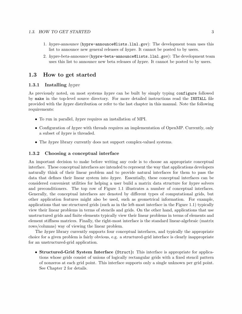
Figure 2.1 gives an example of the type of grid currently supported by the Struct interface.The interface uses a finite-difference or finite-volume style, and currently supports only scalar PDEs(i.e., one unknown per gridpoint). There are four basic steps involved in setting up the linear systemto be solved:
1. set up the grid,
2. set up the stencil,
3. set up the matrix,
4. set up the right-hand-side vector.
(-3,1)
(6,4)
process 0 process 1
Figure 2.1: An example 2D structured grid, distributed accross two processors.
7

8 CHAPTER 2. STRUCTURED-GRID SYSTEM INTERFACE (STRUCT)
(-3,2)
(6,11)
(7,3) (15,8)
Index Space
Figure 2.2: A box is a collection of abstract cell-centered indices, described by its minimum andmaximum indices. Here, two boxes are illustrated.
To describe each of these steps in more detail, consider solving the 2D Laplacian problem
{∇2u = f, in the domain,u = 0, on the boundary.
(2.1)
Assume (2.1) is discretized using standard 5-pt finite-volumes on the uniform grid pictured in 2.1,and assume that the problem data is distributed across two processes as depicted.
2.1 Setting Up the Struct Grid
The grid is described via a global index space, i.e., via integer singles in 1D, tuples in 2D, or triplesin 3D (see Figure 2.2). The integers may have any value, negative or positive. The global indexesallow hypre to discern how data is related spatially, and how it is distributed across the parallelmachine. The basic component of the grid is a box: a collection of abstract cell-centered indices inindex space, described by its “lower” and “upper” corner indices. The scalar grid data is alwaysassociated with cell centers, unlike the more general SStruct interface which allows data to beassociated with box indices in several different ways.
Each process describes that portion of the grid that it “owns”, one box at a time. For example,the global grid in Figure 2.1 can be described in terms of three boxes, two owned by process 0, andone owned by process 1. Figure 2.3 shows the code for setting up the grid on process 0 (the code forprocess 1 is similar). The “icons” at the top of the figure illustrate the result of the numbered linesof code. The Create() routine creates an empty 2D grid object that lives on the MPI_COMM_WORLDcommunicator. The SetExtents() routine adds a new box to the grid. The Assemble() routineis a collective call (i.e., must be called on all processes from a common synchronization point), andfinalizes the grid assembly, making the grid “ready to use”.

2.1. SETTING UP THE STRUCT GRID 9
(-3,1)
(2,4)
1(-3,1)
2(-3,1)
(2,4)
3(-3,1)
(2,4)
4
HYPRE_StructGrid grid;int ndim = 2;int ilower[][2] = {{-3,1}, {0,1}};int iupper[][2] = {{-1,2}, {2,4}};
/* Create the grid object */1: HYPRE_StructGridCreate(MPI_COMM_WORLD, ndim, &grid);
/* Set grid extents for the first box */2: HYPRE_StructGridSetExtents(grid, ilower[0], iupper[0]);
/* Set grid extents for the second box */3: HYPRE_StructGridSetExtents(grid, ilower[1], iupper[1]);
/* Assemble the grid */4: HYPRE_StructGridAssemble(grid);
Figure 2.3: Code on process 0 for setting up the grid in Figure 2.1.

10 CHAPTER 2. STRUCTURED-GRID SYSTEM INTERFACE (STRUCT)
0 1 2 3 4
( 0, 0) ( - 1, 0) ( 1, 0) ( 0, - 1) ( 0, 1) st
enci
l ent
ries
offsets
(-1,-1)
(0,0)
0 1
4
2
3
Figure 2.4: Representation of the 5-point discretization stencil for the example problem.
2.2 Setting Up the Struct Stencil
The geometry of the discretization stencil is described by an array of indexes, each representing arelative offset from any given gridpoint on the grid. For example, the geometry of the 5-pt stencilfor the example problem being considered can be represented by the list of index offsets shown inFigure 2.4. Here, the (0, 0) entry represents the “center” coefficient, and is the 0th stencil entry.The (0,−1) entry represents the “south” coefficient, and is the 3rd stencil entry. And so on.
On process 0 or 1, the code in Figure 2.5 will set up the stencil in Figure 2.4. The stencil mustbe the same on all processes. The Create() routine creates an empty 2D, 5-pt stencil object. TheSetElement() routine defines the geometry of the stencil and assigns the stencil numbers for eachof the stencil entries. None of the calls are collective calls.
2.3 Setting Up the Struct Matrix
The matrix is set up in terms of the grid and stencil objects described in Sections 2.1 and 2.2.The coefficients associated with each stencil entry will typically vary from gridpoint to gridpoint,but in the example problem being considered, they are as follows over the entire grid (except atboundaries; see below): −1
−1 4 −1−1
. (2.2)
On process 0, the code in Figure 2.6 will set up matrix values associated with the center (entry0) and south (entry 3) stencil entries as given by 2.2 and Figure 2.6 (boundaries are ignored heretemporarily). The Create() routine creates an empty matrix object. The Initialize() routineindicates that the matrix coefficients (or values) are ready to be set. This routine may or maynot involve the allocation of memory for the coefficient data, depending on the implementation.The optional Set routines mentioned later in this chapter and in the Reference Manual, shouldbe called before this step. The SetBoxValues() routine sets the matrix coefficients for some setof stencil entries over the gridpoints in some box. Note that the box need not correspond to anyof the boxes used to create the grid, but values should be set for all gridpoints that this process

2.3. SETTING UP THE STRUCT MATRIX 11
(-1,-1)
(0,0)
1
(-1,-1)
(0,0)
0
2
(-1,-1)
(0,0)
0 1
3
(-1,-1)
(0,0)
0 1 2
4
(-1,-1)
(0,0)
0 1 2
3
5
(-1,-1)
(0,0)
0 1
4
2
3
6
HYPRE_StructStencil stencil;int ndim = 2;int size = 5;int entry;int offsets[][2] = {{0,0}, {-1,0}, {1,0}, {0,-1}, {0,1}};
/* Create the stencil object */1: HYPRE_StructStencilCreate(ndim, size, &stencil);
/* Set stencil entries */for (entry = 0; entry < size; entry++){
2-6: HYPRE_StructStencilSetElement(stencil, entry, offsets[entry]);}
/* Thats it! There is no assemble routine */
Figure 2.5: Code for setting up the stencil in Figure 2.4.

12 CHAPTER 2. STRUCTURED-GRID SYSTEM INTERFACE (STRUCT)
HYPRE_StructMatrix A;double values[36];int stencil_indices[2] = {0,3};int i;
HYPRE_StructMatrixCreate(MPI_COMM_WORLD, grid, stencil, &A);HYPRE_StructMatrixInitialize(A);
for (i = 0; i < 36; i += 2){
values[i] = 4.0;values[i+1] = -1.0;
}
HYPRE_StructMatrixSetBoxValues(A, ilower[0], iupper[0], 2,stencil_indices, values);
HYPRE_StructMatrixSetBoxValues(A, ilower[1], iupper[1], 2,stencil_indices, values);
/* set boundary conditions */...
HYPRE_StructMatrixAssemble(A);
Figure 2.6: Code for setting up matrix values associated with stencil entries 0 and 3 as given by2.2 and Figure 2.4.

2.4. SETTING UP THE STRUCT RIGHT-HAND-SIDE VECTOR 13
int ilower[2] = {-3, 1};int iupper[2] = { 2, 1};
/* create matrix and set interior coefficients */...
/* implement boundary conditions */...
for (i = 0; i < 12; i++){
values[i] = 0.0;}
i = 3;HYPRE_StructMatrixSetBoxValues(A, ilower, iupper, 1, &i, values);
/* complete implementation of boundary conditions */...
Figure 2.7: Code for adjusting boundary conditions along the lower grid boundary in Figure 2.1.
“owns”. The Assemble() routine is a collective call, and finalizes the matrix assembly, making thematrix “ready to use”.
Matrix coefficients that reach outside of the boundary should be set to zero. For efficiencyreasons, hypre does not do this automatically. The most natural time to insure this is when theboundary conditions are being set, and this is most naturally done after the coefficients on thegrid’s interior have been set. For example, during the implementation of the Dirichlet boundarycondition on the lower boundary of the grid in Figure 2.1, the “south” coefficient must be set tozero. To do this on process 0, the code in Figure 2.7 could be used:
2.4 Setting Up the Struct Right-Hand-Side Vector
The right-hand-side vector is set up similarly to the matrix set up described in Section 2.3 above.The main difference is that there is no stencil (note that a stencil currently does appear in theinterface, but this will eventually be removed).
On process 0, the code in Figure 2.8 will set up the right-hand-side vector values. The Create()routine creates an empty vector object. The Initialize() routine indicates that the vector co-efficients (or values) are ready to be set. This routine follows the same rules as its correspondingMatrix routine. The SetBoxValues() routine sets the vector coefficients over the gridpoints insome box, and again, follows the same rules as its corresponding Matrix routine. The Assemble()

14 CHAPTER 2. STRUCTURED-GRID SYSTEM INTERFACE (STRUCT)
HYPRE_StructVector b;double values[18];int i;
HYPRE_StructVectorCreate(MPI_COMM_WORLD, grid, &b);HYPRE_StructVectorInitialize(b);
for (i = 0; i < 18; i++){
values[i] = 0.0;}
HYPRE_StructVectorSetBoxValues(b, ilower[0], iupper[0], values);HYPRE_StructVectorSetBoxValues(b, ilower[1], iupper[1], values);
HYPRE_StructVectorAssemble(b);
Figure 2.8: Code for setting up right-hand-side vector values.
routine is a collective call, and finalizes the vector assembly, making the vector “ready to use”.
2.5 Symmetric Matrices
Some solvers and matrix storage schemes provide capabilities for significantly reducing memoryusage when the coefficient matrix is symmetric. In this situation, each off-diagonal coefficientappears twice in the matrix, but only one copy needs to be stored. The Struct interface providessupport for matrix and solver implementations that use symmetric storage via the SetSymmetric()routine.
To describe this in more detail, consider again the 5-pt finite-volume discretization of (2.1) onthe grid pictured in Figure 2.1. Because the discretization is symmetric, only half of the off-diagonalcoefficients need to be stored. To turn symmetric storage on, the following line of code needs to beinserted somewhere between the Create() and Initialize() calls.
HYPRE_StructMatrixSetSymmetric(A, 1);
The coefficients for the entire stencil can be passed in as before. Note that symmetric storage mayor may not actually be used, depending on the underlying storage scheme. Currently in hypre, theStruct interface always uses symmetric storage.
To most efficiently utilize the Struct interface for symmetric matrices, notice that only half ofthe off-diagonal coefficients need to be set. To do this for the example being considered, we simply

2.5. SYMMETRIC MATRICES 15
need to redefine the 5-pt stencil of Section 2.2 to an “appropriate” 3-pt stencil, then set matrixcoefficients (as in Section 2.3) for these three stencil elements only. For example, we could use thefollowing stencil (0, 1)
(0, 0) (1, 0)
. (2.3)
This 3-pt stencil provides enough information to recover the full 5-pt stencil geometry and associatedmatrix coefficients.

16 CHAPTER 2. STRUCTURED-GRID SYSTEM INTERFACE (STRUCT)
Chapter 3
Semi-Structured-Grid SystemInterface (SStruct)
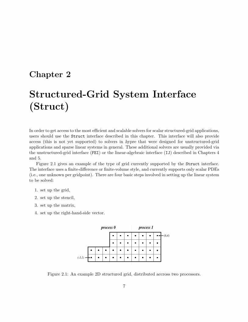
The SStruct interface is appropriate for applications with grids that are mostly—but not entirely—structured, e.g. block-structured grids (see Figure 3.2), composite grids in structured adaptivemesh refinement (AMR) applications (see Figure 3.7), and overset grids. In addition, it supportsmore general PDEs than the Struct interface by allowing multiple variables (system PDEs) andmultiple variable types (e.g. cell-centered, face-centered, etc.). The interface provides access todata structures and linear solvers in hypre that are designed for semi-structured grid problems, butalso to the most general data structures and solvers. These latter solvers are usually provided viathe FEI or IJ interfaces described in Chapters 4 and 5.
The SStruct grid is composed out of a number of structured grid parts, where the physical inter-relationship between the parts is arbitrary. Each part is constructed out of two basic components:boxes (see Figure 2.2) and variables. Variables represent the actual unknown quantities in thegrid, and are associated with the box indices in a variety of ways, depending on their types. Inhypre, variables may be cell-centered, node-centered, face-centered, or edge-centered. Face-centeredvariables are split into x-face, y-face, and z-face, and edge-centered variables are split into x-edge,y-edge, and z-edge. See Figure 3.1 for an illustration in 2D.
The SStruct interface uses a graph to allow nearly arbitrary relationships between part data.The graph is constructed from stencils plus some additional data-coupling information set by theGraphAddEntries() routine. Another method for relating part data is the GridSetNeighborbox()routine, which is particularly suited for block-structured grid problems.
There are five basic steps involved in setting up the linear system to be solved:
1. set up the grid,
2. set up the stencils,
3. set up the graph,
4. set up the matrix,
5. set up the right-hand-side vector.
17

18 CHAPTER 3. SEMI-STRUCTURED-GRID SYSTEM INTERFACE (SSTRUCT)
(i, j )
Figure 3.1: Grid variables in hypre are referenced by the abstract cell-centered index to the leftand down in 2D (analogously in 3D). In the figure, index (i, j) is used to reference the variables inblack. The variables in grey—although contained in the pictured cell—are not referenced by the(i, j) index.
3.1 Block-Structured Grids
In this section, we describe how to use the SStruct interface to define block-structured grid prob-lems. We will do this primarily by example, paying particular attention to the construction ofstencils and the use of the GridSetNeighborbox() interface routine.
Consider the solution of the diffusion equation
−∇ · (D∇u) + σu = f (3.1)
on the block-structured grid in Figure 3.2, where D is a scalar diffusion coefficient, and σ ≥ 0.The discretization [17] introduces three different types of variables: cell-centered, x-face, and y-face. The three discretization stencils that couple these variables are also given in the figure. Theinformation in this figure is essentially all that is needed to describe the nonzero structure of thelinear system we wish to solve.
The grid in Figure 3.2 is defined in terms of five separate logically-rectangular parts as shown inFigure 3.3, and each part is given a unique label between 0 and 4. Each part consists of a single boxwith lower index (1, 1) and upper index (4, 4) (see Section 2.1), and the grid data is distributed onfive processes such that data associated with part p lives on process p. Note that in general, partsmay be composed out of arbitrary unions of boxes, and indices may consist of non-positive integers(see Figure 2.2). Also note that the SStruct interface expects a domain-based data distributionby boxes, but the actual distribution is determined by the user and simply described (in parallel)through the interface.
As with the Struct interface, each process describes that portion of the grid that it “owns”,one box at a time. Figure 3.4 shows the code for setting up the grid on process 3 (the code for theother processes is similar). The “icons” at the top of the figure illustrate the result of the numberedlines of code. Process 3 needs to describe the data pictured in the bottom-right of the figure. Thatis, it needs to describe part 3 plus some additional neighbor information that ties part 3 together
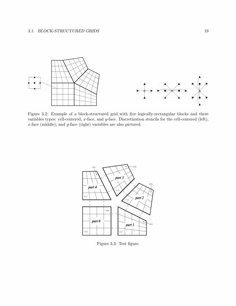
3.1. BLOCK-STRUCTURED GRIDS 19
Figure 3.2: Example of a block-structured grid with five logically-rectangular blocks and threevariables types: cell-centered, x-face, and y-face. Discretization stencils for the cell-centered (left),x-face (middle), and y-face (right) variables are also pictured.
(1,1) (1,1)
(1,1)
(1,1)
(1,1)
(4,4)
(4,4)
(4,4)
(4,4)
part 0 part 1
part 2
part 3
part 4
(4,4)
Figure 3.3: Test figure.

20 CHAPTER 3. SEMI-STRUCTURED-GRID SYSTEM INTERFACE (SSTRUCT)
(1,1)
(1,4)
(4,1)
(4,4)
(1,1)
(4,4)
part 2
part 3 part 4
1
(1,1)
(4,4)
part 3
(1,1)
(4,4)
part 3
2
(1,1)
(4,4)
part 3
(1,1)
(4,4)
part 3
3
(1,1)
(1,4)
(1,1)
(4,4)
part 2
part 3
(1,1)
(1,4)
(1,1)
(4,4)
part 2
part 3
4
(1,1)
(1,4)
(4,1)
(4,4)
(1,1)
(4,4)
part 2
part 3 part 4
(1,1)
(1,4)
(4,1)
(4,4)
(1,1)
(4,4)
part 2
part 3 part 4
5
(1,1)
(1,4)
(4,1)
(4,4)
(1,1)
(4,4)
part 2
part 3 part 4
(1,1)
(1,4)
(4,1)
(4,4)
(1,1)
(4,4)
part 2
part 3 part 4
6
HYPRE_SStructGrid grid;int ndim = 2, nparts = 5, nvars = 3, part = 3;int extents[][2] = {{1,1}, {4,4}};int vartypes[] = {HYPRE_SSTRUCT_VARIABLE_CELL,
HYPRE_SSTRUCT_VARIABLE_XFACE,HYPRE_SSTRUCT_VARIABLE_YFACE};
int nb2_n_part = 2, nb4_n_part = 4;int nb2_exts[][2] = {{1,0}, {4,0}}, nb4_exts[][2] = {{0,1}, {0,4}};int nb2_n_exts[][2] = {{1,1}, {1,4}}, nb4_n_exts[][2] = {{4,1}, {4,4}};int nb2_map[2] = {1,0}, nb4_map[2] = {0,1};
1: HYPRE_SStructGridCreate(MPI_COMM_WORLD, ndim, nparts, &grid);
/* Set grid extents and grid variables for part 3 */2: HYPRE_SStructGridSetExtents(grid, part, extents[0], extents[1]);3: HYPRE_SStructGridSetVariables(grid, part, nvars, vartypes);
/* Set spatial relationship between parts 3 and 2, then parts 3 and 4 */4: HYPRE_SStructGridSetNeighborBox(grid, part, nb2_exts[0], nb2_exts[1],
nb2_n_part, nb2_n_exts[0], nb2_n_exts[1], nb2_map);5: HYPRE_SStructGridSetNeighborBox(grid, part, nb4_exts[0], nb4_exts[1],
nb4_n_part, nb4_n_exts[0], nb4_n_exts[1], nb4_map);
6: HYPRE_SStructGridAssemble(grid);
Figure 3.4: Code on process 3 for setting up the grid in Figure 3.2.

3.1. BLOCK-STRUCTURED GRIDS 21
with the rest of the grid. The Create() routine creates an empty 2D grid object with five partsthat lives on the MPI_COMM_WORLD communicator. The SetExtents() routine adds a new box tothe grid. The SetVariables() routine associates three variables of type cell-centered, x-face, andy-face with part 3.
At this stage, the description of the data on part 3 is complete. However, the spatial relationshipbetween this data and the data on neighboring parts is not yet defined. To do this, we need to relatethe index space for part 3 with the index spaces of parts 2 and 4. More specifically, we need totell the interface that the two grey boxes neighboring part 3 in the bottom-right of Figure 3.4 alsocorrespond to boxes on parts 2 and 4. This is done through the two calls to the SetNeighborbox()routine. We will discuss only the first call, which describes the grey box on the right of the figure.Note that this grey box lives outside of the box extents for the grid on part 3, but it can still bedescribed using the index-space for part 3 (recall Figure 2.2). That is, the grey box has extents(1, 0) and (4, 0) on part 3’s index-space, which is outside of part 3’s grid. The arguments for theSetNeighborbox() call are simply the lower and upper indices on part 3 and the correspondingindices on part 2. The final argument to the routine indicates that the x-direction on part 3 (i.e.,the i component of the tuple (i, j)) corresponds to the y-direction on part 2 and that the y-directionon part 3 corresponds to the x-direction on part 2.
The Assemble() routine is a collective call (i.e., must be called on all processes from a commonsynchronization point), and finalizes the grid assembly, making the grid “ready to use”.
With the neighbor information, it is now possible to determine where off-part stencil entriescouple. Take, for example, any shared part boundary such as the boundary between parts 2 and 3.Along these boundaries, some stencil entries reach outside of the part. If no neighbor informationis given, these entries are effectively zeroed out, i.e., they don’t participate in the discretization.However, with the additional neighbor information, when a stencil entry reaches into a neighborbox it is then coupled to the part described by that neighbor box information.
Another important consequence of the use of the SetNeighborbox() routine is that it can de-clare variables on different parts as being the same. For example, the face variables on the boundaryof parts 2 and 3 are recognized as being shared by both parts (prior to the SetNeighborbox() call,there were two distinct sets of variables). Note also that these variables are of different types onthe two parts; on part 2 they are x-face variables, but on part 3 they are y-face variables.
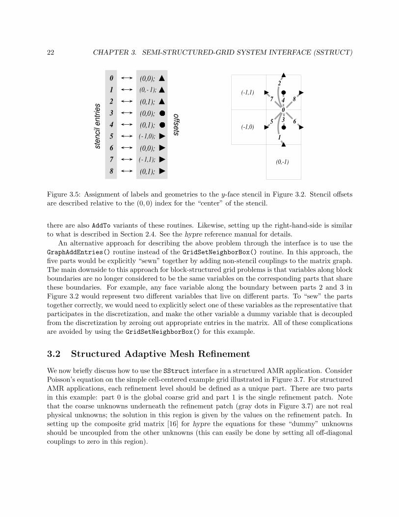
For brevity, we consider only the description of the y-face stencil in Figure 3.2, i.e. the thirdstencil in the figure. To do this, the stencil entries are assigned unique labels between 0 and 8 andtheir “offsets” are described relative to the “center” of the stencil. This process is illustrated inFigure 3.5. Nine calls are made to the routine HYPRE_SStructStencilSetEntry(). As an example,the call that describes stencil entry 5 in the figure is given the entry number 5, the offset (−1, 0),and the identifier for the x-face variable (the variable to which this entry couples). Recall fromFigure 3.1 the convention used for referencing variables of different types. The geometry descriptionuses the same convention, but with indices numbered relative to the referencing index (0, 0) for thestencil’s center. Figure 3.6 shows the code for setting up the graph .
With the above, we now have a complete description of the nonzero structure for the matrix. Thematrix coefficients are then easily set in a manner similar to what is described in Section 2.3 usingroutines MatrixSetValues() and MatrixSetBoxValues() in the SStruct interface. As before,
22 CHAPTER 3. SEMI-STRUCTURED-GRID SYSTEM INTERFACE (SSTRUCT)
0 1 2 3 4 5 6 7 8
(0,0); (0, - 1);
(0,1);
(0,0);
(0,1); ( - 1,0);
(0,0); ( - 1,1);
(0,1);
sten
cil e
ntrie
s
offsets
(-1,1)
(-1,0)
(0,-1)
0
1
2
3
4
5 6
7 8
Figure 3.5: Assignment of labels and geometries to the y-face stencil in Figure 3.2. Stencil offsetsare described relative to the (0, 0) index for the “center” of the stencil.
there are also AddTo variants of these routines. Likewise, setting up the right-hand-side is similarto what is described in Section 2.4. See the hypre reference manual for details.
An alternative approach for describing the above problem through the interface is to use theGraphAddEntries() routine instead of the GridSetNeighborBox() routine. In this approach, thefive parts would be explicitly “sewn” together by adding non-stencil couplings to the matrix graph.The main downside to this approach for block-structured grid problems is that variables along blockboundaries are no longer considered to be the same variables on the corresponding parts that sharethese boundaries. For example, any face variable along the boundary between parts 2 and 3 inFigure 3.2 would represent two different variables that live on different parts. To “sew” the partstogether correctly, we would need to explicitly select one of these variables as the representative thatparticipates in the discretization, and make the other variable a dummy variable that is decoupledfrom the discretization by zeroing out appropriate entries in the matrix. All of these complicationsare avoided by using the GridSetNeighborBox() for this example.
3.2 Structured Adaptive Mesh Refinement
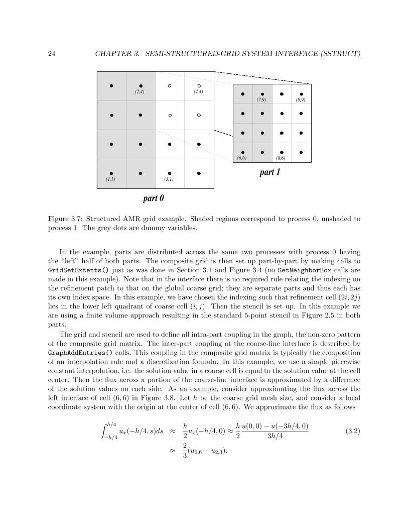
We now briefly discuss how to use the SStruct interface in a structured AMR application. ConsiderPoisson’s equation on the simple cell-centered example grid illustrated in Figure 3.7. For structuredAMR applications, each refinement level should be defined as a unique part. There are two partsin this example: part 0 is the global coarse grid and part 1 is the single refinement patch. Notethat the coarse unknowns underneath the refinement patch (gray dots in Figure 3.7) are not realphysical unknowns; the solution in this region is given by the values on the refinement patch. Insetting up the composite grid matrix [16] for hypre the equations for these “dummy” unknownsshould be uncoupled from the other unknowns (this can easily be done by setting all off-diagonalcouplings to zero in this region).

3.2. STRUCTURED ADAPTIVE MESH REFINEMENT 23
1 2 3
4 5
HYPRE_SStructGraph graph;HYPRE_SStructStencil c_stencil, x_stencil, y_stencil;int c_var = 0, x_var = 1, y_var = 2;int part;
/* Create the graph object */1: HYPRE_SStructGraphCreate(MPI_COMM_WORLD, grid, &graph);
/* Set the cell-centered, x-face, and y-face stencils for each part */for (part = 0; part < 5; part++){
2: HYPRE_SStructGraphSetStencil(graph, part, c_var, c_stencil);3: HYPRE_SStructGraphSetStencil(graph, part, x_var, x_stencil);4: HYPRE_SStructGraphSetStencil(graph, part, y_var, y_stencil);
}
/* No need to add non-stencil entries in this example */5: HYPRE_SStructGraphAssemble(graph);
Figure 3.6: Test figure.
24 CHAPTER 3. SEMI-STRUCTURED-GRID SYSTEM INTERFACE (SSTRUCT)
(4,4)
(1,1)
(2,4)
(3,1)
(9,9)
(6,6)
(7,9)
(8,6)
part 0
part 1
Figure 3.7: Structured AMR grid example. Shaded regions correspond to process 0, unshaded toprocess 1. The grey dots are dummy variables.
In the example, parts are distributed across the same two processes with process 0 havingthe “left” half of both parts. The composite grid is then set up part-by-part by making calls toGridSetExtents() just as was done in Section 3.1 and Figure 3.4 (no SetNeighborBox calls aremade in this example). Note that in the interface there is no required rule relating the indexing onthe refinement patch to that on the global coarse grid; they are separate parts and thus each hasits own index space. In this example, we have chosen the indexing such that refinement cell (2i, 2j)lies in the lower left quadrant of coarse cell (i, j). Then the stencil is set up. In this example weare using a finite volume approach resulting in the standard 5-point stencil in Figure 2.5 in bothparts.
The grid and stencil are used to define all intra-part coupling in the graph, the non-zero patternof the composite grid matrix. The inter-part coupling at the coarse-fine interface is described byGraphAddEntries() calls. This coupling in the composite grid matrix is typically the compositionof an interpolation rule and a discretization formula. In this example, we use a simple piecewiseconstant interpolation, i.e. the solution value in a coarse cell is equal to the solution value at the cellcenter. Then the flux across a portion of the coarse-fine interface is approximated by a differenceof the solution values on each side. As an example, consider approximating the flux across theleft interface of cell (6, 6) in Figure 3.8. Let h be the coarse grid mesh size, and consider a localcoordinate system with the origin at the center of cell (6, 6). We approximate the flux as follows
∫ h/4
−h/4ux(−h/4, s)ds ≈ h
2ux(−h/4, 0) ≈ h
2u(0, 0)− u(−3h/4, 0)
3h/4(3.2)
≈ 23(u6,6 − u2,3).

3.2. STRUCTURED ADAPTIVE MESH REFINEMENT 25
(3,2)
(2,3) (6,6)
Figure 3.8: Coupling for equation at corner of refinement patch. Black lines (solid and broken) arestencil couplings. Gray line are non-stencil couplings.
The first approximation uses the midpoint rule for the edge integral, the second uses a finitedifference formula for the derivative, and the third the piecewise constant interpolation to thesolution in the coarse cell. This means that the equation for the variable at cell (6, 6) involvesnot only the stencil couplings to (6, 7) and (7, 6) on part 1 but also non-stencil couplings to (2, 3)and (3, 2) on part 0. These non-stencil couplings are described by GraphAddEntries() calls. Thesyntax for this call is simply the part and index for both the variable whose equation is being definedand the variable to which it couples. After these calls, the non-zero pattern of the matrix (and thegraph) is complete. Note that the “west” and “south” stencil couplings simply “drop off” the part,and are effectively zeroed out (currently, this is only supported for the HYPRE_PARCSR object type,and these values must be manually zeroed out for other object types; see MatrixSetObjectType()in the reference manual).
The remaining step is to define the actual numerical values for the composite grid matrix.This can be done by either MatrixSetValues() calls to set entries in a single equation, or byMatrixSetBoxValues() calls to set entries for a box of equations in a single call. The syntax forthe MatrixSetValues() call is a part and index for the variable whose equation is being set and anarray of entry numbers identifying which entries in that equation are being set. The entry numbersmay correspond to stencil entries or non-stencil entries.

26 CHAPTER 3. SEMI-STRUCTURED-GRID SYSTEM INTERFACE (SSTRUCT)

Chapter 4
Finite Element Interface
4.1 Introduction
Many application codes use unstructured finite element meshes. This section describes an interfacefor finite element problems, called the FEI, which is supported in hypre.
Figure 4.1: Example of an unstructured mesh.
FEI refers to a specific interface for black-box finite element solvers, originally developed inSandia National Lab, see [6]. It differs from the rest of the conceptual interfaces in hypre in twoimportant aspects: it is written in C++, and it does not separate the construction of the linearsystem matrix from the solution process. A complete description of Sandia’s FEI implementationcan be obtained by contacting Alan Williams at Sandia ([email protected]). A simplified versionof the FEI has been implemented at LLNL and is included in hypre. More details about thisimplementation can be found in the header files of the FEI_mv/fei-base and FEI_mv/fei-hypredirectories.
27

28 CHAPTER 4. FINITE ELEMENT INTERFACE
4.2 A Brief Description of the Finite Element Interface
Typically, finite element codes contain data structures storing element connectivities, element stiff-ness matrices, element loads, boundary conditions, nodal coordinates, etc. One of the purposes ofthe FEI is to assemble the global linear system in parallel based on such local element data. Weillustrate this in the rest of the section and refer to example 10 (in the examples directory) formore implementation details.
In hypre, one creates an instance of the FEI as follows:
LLNL_FEI_Impl *feiPtr = new LLNL_FEI_Impl(mpiComm);
Here mpiComm is an MPI communicator (e.g. MPI COMM WORLD). If Sandia’s FEI package is to beused, one needs to define a hypre solver object first:
LinearSystemCore *solver = HYPRE_base_create(mpiComm);FEI_Implementation *feiPtr = FEI_Implementation(solver,mpiComm,rank);
where rank is the number of the master processor (used only to identify which processor willproduce the screen outputs). The LinearSystemCore class is the part of the FEI which interfaceswith the linear solver library. It will be discussed later in Sections 6.14 and 7.7.
Local finite element information is passed to the FEI using several methods of the feiPtr object.The first entity to be submitted is the field information. A field has an identifier called fieldID anda rank or fieldSize (number of degree of freedom). For example, a discretization of the NavierStokes equations in 3D can consist of velocity vector having 3 degrees of freedom in every node(vertex) of the mesh and a scalar pressure variable, which is constant over each element. If theseare the only variables, and if we assign fieldIDs 7 and 8 to them, respectively, then the finiteelement field information can be set up by
nFields = 2; /* number of unknown fields */fieldID = new int[nFields]; /* field identifiers */fieldSize = new int[nFields]; /* vector dimension of each field */
/* velocity (a 3D vector) */fieldID[0] = 7;fieldSize[0] = 3;
/* pressure (a scalar function) */fieldID[1] = 8;fieldSize[1] = 1;
feiPtr -> initFields(nFields, fieldSize, fieldID);
Once the field information has been established, we are ready to initialize an element block.An element block is characterized by the block identifier, the number of elements, the number ofnodes per element, the nodal fields and the element fields (fields that have been defined previously).Suppose we use 1000 hexahedral elements in the element block 0, the setup consists of

4.2. A BRIEF DESCRIPTION OF THE FINITE ELEMENT INTERFACE 29
elemBlkID = 0; /* identifier for a block of elements */nElems = 1000; /* number of elements in the block */elemNNodes = 8; /* number of nodes per element */
/* nodal-based field for the velocity */nodeNFields = 1;nodeFieldIDs = new[nodeNFields];nodeFieldIDs[0] = fieldID[0];
/* element-based field for the pressure */elemNFields = 1;elemFieldIDs = new[elemNFields];elemFieldIDs[0] = fieldID[1];
feiPtr -> initElemBlock(elemBlkID, nElems, elemNNodes, nodeNFields,nodeFieldIDs, elemNFields, elemFieldIDs, 0);
The last argument above specifies how the dependent variables are arranged in the element matrices.A value of 0 indicates that each variable is to be arranged in a separate block (as opposed tointerleaving).
In a parallel environment, each processor has one or more element blocks. Unless the elementblocks are all disjoint, some of them share a common set of nodes on the subdomain boundaries. Tofacilitate setting up interprocessor communications, shared nodes between subdomains on differentprocessors are to be identified and sent to the FEI. Hence, each node in the whole domain is assigneda unique global identifier. The shared node list on each processor contains a subset of the globalnode list corresponding to the local nodes that are shared with the other processors. The syntaxfor setting up the shared nodes is
feiPtr -> initSharedNodes(nShared, sharedIDs, sharedLengs, sharedProcs);
This completes the initialization phase, and a completion signal is sent to the FEI via
feiPtr -> initComplete();
Next, we begin the load phase. The first entity for loading is the nodal boundary conditions.Here we need to specify the number of boundary equations and the boundary values given byalpha, beta, and gamma. Depending on whether the boundary conditions are Dirichlet, Neumann,or mixed, the three values should be passed into the FEI accordingly.
feiPtr -> loadNodeBCs(nBCs, BCEqn, fieldID, alpha, beta, gamma);
The element stiffness matrices are to be loaded in the next step. We need to specify the elementnumber i, the element block to which element i belongs, the element connectivity information, theelement load, and the element matrix format. The element connectivity specifies a set of 8 nodeglobal IDs (for hexahedral elements), and the element load is the load or force for each degree offreedom. The element format specifies how the equations are arranged (similar to the interleavingscheme mentioned above). The calling sequence for loading element stiffness matrices is

30 CHAPTER 4. FINITE ELEMENT INTERFACE
for (i = 0; i < nElems; i++)feiPtr -> sumInElem(elemBlkID, elemID, elemConn[i], elemStiff[i],
elemLoads[i], elemFormat);
To complete the assembling of the global stiffness matrix and the corresponding right hand side, asignal is sent to the FEI via
feiPtr -> loadComplete();

Chapter 5
Linear-Algebraic System Interface(IJ)
The IJ interface described in this chapter is the lowest common denominator for specifying linearsystems in hypre. This interface provides access to general sparse-matrix solvers in hypre, not tothe specialized solvers that require more problem information.
5.1 IJ Matrix Interface
As with the other interfaces in hypre, the IJ interface expects to get data in distributed form becausethis is the only scalable approach for assembling matrices on thousands of processes. Matrices areassumed to be distributed by blocks of rows as follows:
A0
A1...
AP−1
(5.1)
In the above example, the matrix is distributed accross the P processes, 0, 1, ..., P − 1 by blocksof rows. Each submatrix Ap is “owned” by a single process and its first and last row numbers aregiven by the global indices ilower and iupper in the Create() call below.
The following example code illustrates the basic usage of the IJ interface for building matrices:
MPI_Comm comm;HYPRE_IJMatrix ij_matrix;HYPRE_ParCSRMatrix parcsr_matrix;int ilower, iupper;int jlower, jupper;int nrows;
31

32 CHAPTER 5. LINEAR-ALGEBRAIC SYSTEM INTERFACE (IJ)
int *ncols;int *rows;int *cols;double *values;
HYPRE_IJMatrixCreate(comm, ilower, iupper, jlower, jupper, &ij_matrix);HYPRE_IJMatrixSetObjectType(ij_matrix, HYPRE_PARCSR);HYPRE_IJMatrixInitialize(ij_matrix);
/* set matrix coefficients */HYPRE_IJMatrixSetValues(ij_matrix, nrows, ncols, rows, cols, values);.../* add-to matrix cofficients, if desired */HYPRE_IJMatrixAddToValues(ij_matrix, nrows, ncols, rows, cols, values);...
HYPRE_IJMatrixAssemble(ij_matrix);HYPRE_IJMatrixGetObject(ij_matrix, (void **) &parcsr_matrix);
The Create() routine creates an empty matrix object that lives on the comm communicator. Thisis a collective call (i.e., must be called on all processes from a common synchronization point),with each process passing its own row extents, ilower and iupper. The row partitioning must becontiguous, i.e., iupper for process i must equal ilower−1 for process i+1. Note that this allowsmatrices to have 0- or 1-based indexing. The parameters jlower and jupper define a columnpartitioning, and should match ilower and iupper when solving square linear systems. See theReference Manual for more information.
The SetObjectType() routine sets the underlying matrix object type to HYPRE_PARCSR (thisis the only object type currently supported). The Initialize() routine indicates that the matrixcoefficients (or values) are ready to be set. This routine may or may not involve the allocation ofmemory for the coefficient data, depending on the implementation. The optional SetRowSizes()and SetDiagOffdSizes() routines mentioned later in this chapter and in the Reference Manual,should be called before this step.
The SetValues() routine sets matrix values for some number of rows (nrows) and some numberof columns in each row (ncols). The actual row and column numbers of the matrix values to beset are given by rows and cols. After the coefficients are set, they can be added to with an AddTo()routine. Each process should set only those matrix values that it “owns” in the data distribution.
The Assemble() routine is a collective call, and finalizes the matrix assembly, making thematrix “ready to use”. The GetObject() routine retrieves the built matrix object so that it canbe passed on to hypre solvers that use the ParCSR internal storage format. Note that this is notan expensive routine; the matrix already exists in ParCSR storage format, and the routine simplyreturns a “handle” or pointer to it. Although we currently only support one underlying data storageformat, in the future several different formats may be supported.

5.2. IJ VECTOR INTERFACE 33
One can preset the row sizes of the matrix in order to reduce the execution time for thematrix specification. One can specify the total number of coefficients for each row, the number ofcoefficients in the row that couple the diagonal unknown to (Diag) unknowns in the same processordomain, and the number of coefficients in the row that couple the diagonal unknown to (Offd)unknowns in other processor domains:
HYPRE_IJMatrixSetRowSizes(ij_matrix, sizes);HYPRE_IJMatrixSetDiagOffdSizes(matrix, diag_sizes, offdiag_sizes);
Once the matrix has been assembled, the sparsity pattern cannot be altered without completelydestroying the matrix object and starting from scratch. However, one can modify the matrix valuesof an already assembled matrix. To do this, first call the Initialize() routine to re-initialize thematrix, then set or add-to values as before, and call the Assemble() routine to re-assemble beforeusing the matrix. Re-initialization and re-assembly are very cheap, essentially a no-op in the currentimplementation of the code.
5.2 IJ Vector Interface
The following example code illustrates the basic usage of the IJ interface for building vectors:
MPI_Comm comm;HYPRE_IJVector ij_vector;HYPRE_ParVector par_vector;int jlower, jupper;int nvalues;int *indices;double *values;
HYPRE_IJVectorCreate(comm, jlower, jupper, &ij_vector);HYPRE_IJVectorSetObjectType(ij_vector, HYPRE_PARCSR);HYPRE_IJVectorInitialize(ij_vector);
/* set vector values */HYPRE_IJVectorSetValues(ij_vector, nvalues, indices, values);...
HYPRE_IJVectorAssemble(ij_vector);HYPRE_IJVectorGetObject(ij_vector, (void **) &par_vector);
The Create() routine creates an empty vector object that lives on the comm communicator. This isa collective call, with each process passing its own index extents, jlower and jupper. The names

34 CHAPTER 5. LINEAR-ALGEBRAIC SYSTEM INTERFACE (IJ)
of these extent parameters begin with a j because we typically think of matrix-vector multipliesas the fundamental operation involving both matrices and vectors. For matrix-vector multiplies,the vector partitioning should match the column partitioning of the matrix (which also uses the jnotation). For linear system solves, these extents will typically match the row partitioning of thematrix as well.
The SetObjectType() routine sets the underlying vector storage type to HYPRE_PARCSR (thisis the only storage type currently supported). The Initialize() routine indicates that the vectorcoefficients (or values) are ready to be set. This routine may or may not involve the allocation ofmemory for the coefficient data, depending on the implementation.
The SetValues() routine sets the vector values for some number (nvalues) of indices. Eachprocess should set only those vector values that it “owns” in the data distribution.
The Assemble() routine is a trivial collective call, and finalizes the vector assembly, makingthe vector “ready to use”. The GetObject() routine retrieves the built vector object so that it canbe passed on to hypre solvers that use the ParVector internal storage format.
Vector values can be modified in much the same way as with matrices by first re-initializing thevector with the Initialize() routine.
5.3 A Scalable Interface
As explained in the previous sections, problem data is passed to the hypre library in its distributedform. However, as is typically the case for a parallel software library, some information regardingthe global distribution of the data will be needed for hypre to perform its function. In particular,a solver algorithm requires that a processor obtain “nearby” data from other processors in orderto complete the solve. While a processor may easily determine what data it needs from otherprocessors, it may not know which processor owns the data it needs. Therefore, processors mustdetermine their communication partners, or neighbors.
The straightforward approach to determining neighbors involves constructing a global partitionof the data which requires O(P ) data storage. This storage requirement (as well the costs of many ofthe associated algorithms that access the storage) is not scalable for machines such as BlueGene/Lwith tens of thousands of processors. The problem of determining inter-processor communication(in the absence of a global description of the data) in a scalable manner is addressed in [2]. Whenusing hypre on many thousands of processors, compiling the library with the “no global partition”option as detailed in Section 7.2.1 improves scalability as shown in [2]. Note that this optimizationis only recommended when using at least several thousand of processors and is most beneficial whenusing tens of thousands of processors.

Chapter 6
Solvers and Preconditioners
There are several solvers available in hypre via different conceptual interfaces (see Table 6.1). Notethat there are a few additional solvers and preconditioners not mentioned in the table that can beused only through the FEI interface and are described in Paragraph 6.14. The procedure for setupand use of solvers and preconditioners is largely the same. We will refer to them both as solversin the sequel except when noted. In normal usage, the preconditioner is chosen and constructedbefore the solver, and then handed to the solver as part of the solver’s setup. In the following, weassume the most common usage pattern in which a single linear system is set up and then solvedwith a single righthand side. We comment later on considerations for other usage patterns.
Setup:
1. Pass to the solver the information defining the problem. In the typical user cycle, theuser has passed this information into a matrix through one of the conceptual interfaces priorto setting up the solver. In this situation, the problem definition information is then passedto the solver by passing the constructed matrix into the solver. As described before, thematrix and solver must be compatible, in that the matrix must provide the services neededby the solver. Krylov solvers, for example, need only a matrix-vector multiplication. Mostpreconditioners, on the other hand, have additional requirements such as access to the matrixcoefficients.
2. Create the solver/preconditioner via the Create() routine.
3. Choose parameters for the preconditioner and/or solver. Parameters are chosenthrough the Set() calls provided by the solver. Throughout hypre, we have made our besteffort to give all parameters reasonable defaults if not chosen. However, for some precondi-tioners/solvers the best choices for parameters depend on the problem to be solved. We giverecommendations in the individual sections on how to choose these parameters. Note that inhypre, convergence criteria can be chosen after the preconditioner/solver has been setup. Fora complete set of all available parameters see the Reference Manual.
35

36 CHAPTER 6. SOLVERS AND PRECONDITIONERS
System InterfacesSolvers Struct SStruct FEI IJ
Jacobi X XSMG X XPFMG X XSysPFMG XSplit XFAC XMaxwell XBoomerAMG X X XAMS X X XMLI X X XParaSails X X XEuclid X X XPILUT X X XPCG X X X XGMRES X X X XBiCGSTAB X X X XHybrid X X X X
Table 6.1: Current solver availability via hypre conceptual interfaces.
4. Pass the preconditioner to the solver. For solvers that are not preconditioned, this stepis omitted. The preconditioner is passed through the SetPrecond() call.
5. Set up the solver. This is just the Setup() routine. At this point the matrix and righthand side is passed into the solver or preconditioner. Note that the actual right hand side isnot used until the actual solve is performed.
At this point, the solver/preconditioner is fully constructed and ready for use.
Use:
1. Set convergence criteria. Convergence can be controlled by the number of iterations,as well as various tolerances such as relative residual, preconditioned residual, etc. Like allparameters, reasonable defaults are used. Users are free to change these, though care must betaken. For example, if an iterative method is used as a preconditioner for a Krylov method,a constant number of iterations is usually required.
2. Solve the system. This is just the Solve() routine.

6.1. SMG 37
Finalize:
1. Free the solver or preconditioner. This is done using the Destroy() routine.
Synopsis
In general, a solver (let’s call it SOLVER) is set up and run using the following routines, where A isthe matrix, b the right hand side and x the solution vector of the linear system to be solved:
/* Create Solver */int HYPRE_SOLVERCreate(MPI_COMM_WORLD, &solver);
/* set certain parameters if desired */HYPRE_SOLVERSetTol(solver, 1.e-8);../* Set up Solver */HYPRE_SOLVERSetup(solver, A, b, x);/* Solve the system */HYPRE_SOLVERSolve(solver, A, b, x);/* Destroy the solver */HYPRE_SOLVERDestroy(solver);
In the following sections, we will give brief descriptions of the available hypre solvers with somesuggestions on how to choose the parameters as well as references for users who are interested ina more detailed description and analysis of the solvers. A complete list of all routines that areavailable can be found in the reference manual.
6.1 SMG
SMG is a parallel semicoarsening multigrid solver for the linear systems arising from finite difference,finite volume, or finite element discretizations of the diffusion equation,
∇ · (D∇u) + σu = f (6.1)
on logically rectangular grids. The code solves both 2D and 3D problems with discretization stencilsof up to 9-point in 2D and up to 27-point in 3D. See [19, 3, 7] for details on the algorithm and itsparallel implementation/performance.
SMG is a particularly robust method. The algorithm semicoarsens in the z-direction and usesplane smoothing. The xy plane-solves are effected by one V-cycle of the 2D SMG algorithm, whichsemicoarsens in the y-direction and uses line smoothing.

38 CHAPTER 6. SOLVERS AND PRECONDITIONERS
6.2 PFMG
PFMG is a parallel semicoarsening multigrid solver similar to SMG. See [1, 7] for details on thealgorithm and its parallel implementation/performance.
The main difference between the two methods is in the smoother: PFMG uses simple pointwisesmoothing. As a result, PFMG is not as robust as SMG, but is much more efficient per V-cycle.
6.3 SysPFMG
SysPFMG is a parallel semicoarsening multigrid solver for systems of elliptic PDEs. It is a gener-alization of PFMG, with the interpolation defined only within the same variable. The relaxation isof nodal type- all variables at a given point location are simultaneously solved for in the relaxation.
Although SysPFMG is implemented through the SStruct interface, it can be used only forproblems with one grid part. Ideally, the solver should handle any of the seven variable types (cell-,node-, xface-, yface-, zface-, xedge-, yedge-, and zedge-based). However, it has been completed onlyfor cell-based variables.
6.4 SplitSolve
SplitSolve is a parallel block Gauss-Seidel solver for semi-structured problems with multiple parts.For problems with only one variable, it can be viewed as a domain-decomposition solver with nogrid overlapping.
Consider a multiple part problem given by the linear system Ax = b. Matrix A can be decom-posed into a structured intra-variable block diagonal component M and a component N consistingof the inter-variable blocks and any unstructured connections between the parts. SplitSolve per-forms the iteration
xk+1 = M−1(b + Nxk),
where M−1 is a decoupled block-diagonal V(1,1) cycle, a separate cycle for each part and variabletype. There are two V-cycle options, SMG and PFMG.
6.5 FAC
FAC is a parallel fast adaptive composite grid solver for finite volume, cell-centred discretizations ofsmooth diffusion coefficient problems. To be precise, it is a FACx algorithm since the patch solvesconsist of only relaxation sweeps. For details of the basic overall algorithms, see [16]. Algorithmicparticularities include formation of non-Galerkin coarse-grid operators (i.e., coarse-grid operatorsunderlying refinement patches are automatically generated) and non-stored linear/constant inter-polation/restriction operators. Implementation particularities include a processor redistributionof the generated coarse-grid operators so that intra-level communication between adaptive meshrefinement (AMR) levels during the solve phase is kept to a minimum. This redistribution is hiddenfrom the user.

6.6. MAXWELL 39
The user input is essentially a linear system describing the composite operator, and the refine-ment factors between the AMR levels. To form this composite linear system, the AMR grid isdescribed using semi-structured grid parts. Each AMR level grid corresponds to a separate partso that this level grid is simply a collection of boxes, all with the same refinement factor, i.e., it isa struct grid. However, several restrictions are imposed on the patch (box) refinements. First, arefinement box must cover all underlying coarse cells- i.e., refinement of a partial coarse cell is notpermitted. Also, the refined/coarse indices must follow a mapping: with [r1, r2, r3] denoting therefinement factor and [a1, a2, a3]× [b1, b2, b3] denoting the coarse subbox to be refined, the mappingto the refined patch is
[r1 ∗ a1, r2 ∗ a2, r3 ∗ a3]× [r1 ∗ b1 + r1 − 1, r2 ∗ b2 + r2 − 1, r3 ∗ b3 + r3 − 1].
With the AMR grid constructed under these restrictions, the composite matrix can be formed.Since the AMR levels correspond to semi-structured grid parts, the composite matrix is a semi-structured matrix consisting of structured components within each part, and unstructured com-ponents describing the coarse-to-fine/fine-to-coarse connections. The structured and unstructuredcomponents can be set using stencils and the HYPRE SStructGraphAddEntries routine, respec-tively. The matrix coefficients can be filled after setting these non-zero patterns. Between eachpair of successive AMR levels, the coarse matrix underlying the refinement patch must be theidentity and the corresponding rows of the rhs must be zero. These can performed using routinesHYPRE SStructFACZeroCFSten (to zero off the stencil values reaching from coarse boxes intorefinement boxes), HYPRE SStructFACZeroFCSten (to zero off the stencil values reaching fromrefinement boxes into coarse boxes), HYPRE SStructFACZeroAMRMatrixData (to set the identityat coarse grid points underlying a refinement patch), and HYPRE SStructFACZeroAMRVectorData(to zero off a vector at coarse grid points underlying a refinement patch). These routines can sim-plify the user’s matrix setup. For example, consider two successive AMR levels with the coarserlevel consisting of one box and the finer level consisting of a collection of boxes. Rather than dis-tinguishly setting the stencil values and the identity in the appropriate locations, the user can setthe stencil values on the whole coarse grid using the HYPRE SStructMatrixSetBoxValues routineand then zero off the appropriate values using the above zeroing routines.
The coarse matrix underlying these patches are algebraically generated by operator-collapsingthe refinement patch operator and the fine-to-coarse coefficients (this is why stencil values reachingout of a part must be zeroed). This matrix is re-distributed so that each processor has all of itscoarse-grid operator.
To solve the coarsest AMR level, a PFMG V cycle is used. Note that a minimum of two AMRlevels are needed for this solver.
6.6 Maxwell
Maxwell is a parallel solver for edge finite element discretization of the curl-curl formulation of theMaxwell equation
∇× α∇× E + βE = f, β > 0

40 CHAPTER 6. SOLVERS AND PRECONDITIONERS
on semi-structured grids. Details of the algorithm can be found in [12]. The solver can be viewedas an operator-dependent multiple-coarsening algorithm for the Helmholtz decomposition of theerror correction. Input to this solver consist of only the linear system and a gradient operator. Infact, if the orientation of the edge elements conforms to a lexigraphical ordering of the nodes of thegrid, then the gradient operator can be generated with the routine HYPRE MaxwellGrad: at gridpoints (i, j, k) and (i− 1, j, k), the produced gradient operator takes values 1 and −1 respectively,which is the correct gradient operator for the appropriate edge orientation. Since the gradientoperator is normalized (i.e., h independent) the edge finite element must also be normalized in thediscretization.
This solver is currently developed for perfectly conducting boundary condition (Dirichlet).Hence, the rows and columns of the matrix that corresponding to the grid boundary must be set tothe identity or zeroed off. This can be achieved with the routines HYPRE SStructMaxwellPhysBdyand HYPRE SStructMaxwellEliminateRowsCols. The former identifies the ranks of the rows thatare located on the grid boundary, and the latter adjusts the boundary rows and cols. As usual,the rhs of the linear system must also be zeroed off at the boundary rows. This can be done usingHYPRE SStructMaxwellZeroVector.
With the adjusted linear system and a gradient operator, the user can form the Maxwellmultigrid solver using several different edge interpolation schemes. For problems with smoothcoefficients, the natural Nedelec interpolation operator can be used. This is formed by callingHYPRE SStructMaxwellSetConstantCoef with the flag> 0 before setting up the solver, otherwisethe default edge interpolation is an operator-collapsing/element-agglomeration scheme. This is suit-able for variable coefficients. Also, before setting up the solver, the user must pass the gradient oper-ator, whether user or HYPRE MaxwellGrad generated, with HYPRE SStructMaxwellSetGrad. Af-ter these preliminary calls, the Maxwell solver can be setup by calling HYPRE SStructMaxwellSetup.
There are two solver cycling schemes that can be used to solve the linear system. To describethese, one needs to consider the augmented system operator
A =
[Aee Aen
Ane Ann
], (6.2)
where Aee is the stiffness matrix corresponding to the above curl-curl formulation, Ann is the nodalPoisson operator created by taking the Galerkin product of Aee and the gradient operator, andAne and Aen are the nodal-edge coupling operators (see [12]). The algorithm for this Maxwellsolver is based on forming a multigrid hierarchy to this augmented system using the block-diagonalinterpolation operator
P =
[Pe 0
0 Pn
],
where Pe and Pn are respectively the edge and nodal interpolation operators determined individ-ually from Aee and Ann. Taking a Galerkin product between A and P produces the next coarseaugmented operator, which also has the nodal-edge coupling operators. Applying this procedure re-cursively produces nodal-edge coupling operators at all levels. Now, the first solver cycling scheme,

6.7. HYBRID 41
HYPRE SStructMaxwellSolve, keeps these coupling operators on all levels of the V-cycle. Thesecond, cheaper scheme, HYPRE SStructMaxwellSolve2, keeps the coupling operators only on thefinest level, i.e., separate edge and nodal V-cycles that couple only on the finest level.
6.7 Hybrid
The hybrid solver is designed to detect whether a multigrid preconditioner is needed when solvinga linear system and possibly avoid the expensive setup of a preconditioner if a system can be solvedefficiently with a diagonally scaled Krylov solver, e.g. a strongly diagonally dominant system.It first uses a diagonally scaled Krylov solver, which can be chosen by the user (the default isconjugate gradient, but one should use GMRES if the matrix of the linear system to be solved isnonsymmetric). It monitors how fast the Krylov solver converges. If there is not sufficient progress,the algorithm switches to a preconditioned Krylov solver.
If used through the Struct interface, the solver is called StructHybrid and can be used with thepreconditioners SMG and PFMG (default). It is called ParCSRHybrid, if used through the IJ inter-face and is used here with BoomerAMG. The user can determine the average convergence speed bysetting a convergence tolerance 0 ≤ θ < 1 via the routine HYPRE StructHybridSetConvergenceTolor HYPRE StructParCSRHybridSetConvergenceTol. The default setting is 0.9.
The average convergence factor ρi =(‖ri‖‖r0‖
)1/iis monitored within the chosen Krylov solver,
where ri = b−Axi is the i-th residual. Convergence is considered too slow when(1− |ρi − ρi−1|
max(ρi, ρi−1)
)ρi > θ. (6.3)
When this condition is fulfilled the hybrid solver switches from a diagonally scaled Krylov solverto a preconditioned solver.
6.8 BoomerAMG
BoomerAMG is a parallel implementation of the algebraic multigrid method [18]. It can be usedboth as a solver or as a preconditioner. The user can choose between various different parallelcoarsening techniques, interpolation and relaxation schemes. See [8, 24] for a detailed descriptionof the coarsening algorithms, interpolation and relaxation schemes as well as numerical results.
6.8.1 Parameter Options
Various BoomerAMG functions and options are mentioned below. However, for a complete listingand description of all available functions, see the reference manual.
BoomerAMG’s Create function differs from the synopsis in that it has only one parameterHYPRE_BoomerAMGCreate(HYPRE_Solver *solver). It uses the communicator of the matrix A.
Coarsening can be set by the user using the function HYPRE BoomerAMGSetCoarsenType. Vari-ous coarsening techniques are available:

42 CHAPTER 6. SOLVERS AND PRECONDITIONERS
• the Cleary-Luby-Jones-Plassman (CLJP) coarsening,
• the Falgout coarsening which is a combination of CLJP and the classical RS coarseningalgorithm (default),
• PMIS and HMIS coarsening algorithms which lead to coarsenings with lower complexities [5]as well as
• aggressive coarsening, which can be applied to any of the coarsening techniques mentionedabove and thus achieving much lower complexities and lower memory use [20].
To use aggressive coarsening the user has to set the number of levels to which he wants to applyaggressive coarsening (starting with the finest level) via HYPRE_BoomerAMGSetAggNumLevels. Sinceaggressive coarsening requires long range interpolation, multipass interpolation is always used onlevels with aggressive coarsening.
Various interpolation techniques can be set using HYPRE_BoomerAMGSetInterpType:
• the “classical” interpolation as defined in [18] (default),
• direct interpolation [20],
• standard interpolation [20],
• multipass interpolation [20],
• an extended “classical” interpolation, which is a long range interpolation and is recommendedto be used with PMIS and HMIS coarsening for harder problems,
• Jacobi interpolation [20],
• the “classical” interpolation modified for hyperbolic PDEs.
Jacobi interpolation is only use to improve certain interpolation operators and can be used withHYPRE_BoomerAMGSetPostInterpType. Since some of the interpolation operators might generatelarge stencils, it is often possible and recommended to control complexity and truncate the interpo-lation operators using HYPRE_BoomerAMGSetTruncFactor and/or HYPRE_BoomerAMGSetPMaxElmts,or HYPRE_BoomerAMGSetJacobiTruncTheshold (for Jacobi interpolation only).
Various relaxation techniques are available:
• weighted Jacobi relaxation,
• a hybrid Gauss-Seidel / Jacobi relaxation scheme,
• a symmetric hybrid Gauss-Seidel / Jacobi relaxation scheme, and
• hybrid block and Schwarz smoothers [23],
• ILU and approximate inverse smoothers.

6.9. AMS 43
Point relaxation schemes can be set using HYPRE_BoomerAMGSetRelaxType or, if one wants to specif-ically set the up cycle, down cycle or the coarsest grid, with HYPRE_BoomerAMGSetCycleRelaxType.To use the more complicated smoothers, e.g. block, Schwarz, ILU smoothers, it is necessary to useHYPRE_BoomerAMGSetSmoothType and HYPRE_BoomerAMGSetSmoothNumLevels. There are furtherparameter choices for the individual smoothers, which are described in the reference manual. Thedefault relaxation type is hybrid Gauss-Seidel with CF-relaxation (relax first the C-, then the F-points) on the down cycle and FC-relaxation on the up-cycle. Note that if BoomerAMG is usedas a preconditioner for comjugate gradient, it is necessary to use a symmetric smoother such asweighted Jacobi or hybrid symmetric Gauss-Seidel.
If the users wants to solve systems of PDEs and can provide information on which variablesbelong to which function, BoomerAMG’s systems AMG version can also be used. Functionsthat enable the user to access the systems AMG version are HYPRE_BoomerAMGSetNumFunctions,HYPRE_BoomerAMGSetDofFunc and HYPRE BoomerAMGSetNodal.
For best performance, it might be necessary to set certain parameters, which will affect bothcoarsening and interpolation. One important parameter is the strong threshold, which can be setusing the function HYPRE_BoomerAMGSetStrongThreshold. The default value is 0.25, which ap-pears to be a good choice for 2-dimensional problems and the low complexity coarsening algorithms.A better choice for 3-dimensional problems appears to be 0.5, if one uses the default coarsening al-gorithm or CLJP. However, the choice of the strength threshold is problem dependent and thereforethere could be better choices than the two suggested ones.
6.9 AMS
AMS (Auxiliary space Maxwell Solver) is a parallel unstructured Maxwell solver for edge finiteelement discretizations of the variational problem
Find u ∈ Vh : (α∇× u,∇× v) + (β u,v) = (f ,v) , for all v ∈ Vh . (6.4)
Here Vh is the lowest order Nedelec (edge) finite element space, and α > 0 and β ≥ 0 are scalar, orSPD matrix coefficients. AMS was designed to be scalable on problems with variable coefficients,and allows for β to be zero in part or the whole domain. In either case the resulting problem isonly semidefinite, and for solvability the right-hand side should be chosen to satisfy compatibilityconditions.
AMS is based on the auxiliary space methods for definite Maxwell problems proposed in [9].For more details, see [15, 14].
6.9.1 Overview
Let A and b be the stiffness matrix and the load vector corresponding to (6.4). Then the resultinglinear system of interest reads,
Ax = b . (6.5)
The coefficients α and β are naturally associated with the “stiffness” and “mass” terms of A.Besides A and b, AMS requires the following additional user input:

44 CHAPTER 6. SOLVERS AND PRECONDITIONERS
1. The discrete gradient matrix G representing the edges of the mesh in terms of its vertices.G has as many rows as the number of edges in the mesh, with each row having two nonzeroentries: +1 and −1 in the columns corresponding to the vertices composing the edge. The signis determined based on the orientation of the edge. We require that G includes all (interiorand boundary) edges and vertices.
2. The representations of the constant vector fields (1, 0, 0),(0, 1, 0) and (0, 0, 1) in the Vh basis,given as three vectors: Gx, Gy, and Gz. Note that since no boundary conditions are imposedon G, the above vectors can be computed as Gx = Gx, Gy = Gy and Gz = Gz, where x, y,and z are vectors representing the coordinates of the vertices of the mesh.
In addition to the above quantities, AMS can utilize the following (optional) information:
(3.) The Poisson matrices Aα and Aβ, corresponding to assembling of the forms (α∇u,∇v) and(β∇u,∇v) using standard linear finite elements on the same mesh.
Internally, AMS proceeds with the construction of the following additional objects:
• AG – a matrix associated with the mass term which is either GTAG, or the Poisson matrixAβ (if given).
• Π – the matrix representation of the interpolation operator from vector linear to edge finiteelements.
• AΠ – a matrix associated with the stiffness term which is either ΠTAΠ or a block-diagonalmatrix with diagonal blocks Aα (if given).
• BG and BΠ – efficient (AMG) solvers for AG and AΠ.
The solution procedure then is a three-level method using smoothing in the original edge spaceand subspace corrections based on BG and BΠ. We can employ a number of options here utilizingvarious combinations of the smoother and solvers in additive or multiplicative fashion. If β isidentically zero one can skip the subspace correction associated with G, in which case the solver isa two-level method.
6.9.2 Sample Usage
AMS can be used either as a solver or as a preconditioner. Below we list the sequence of hypre callsneeded to create and use it as a solver. We start with the allocation of the HYPRE_Solver object:
HYPRE_Solver solver;HYPRE_AMSCreate(&solver);
Next, we set a number of solver parameters. Some of them are optional, while others arenecessary in order to perform the solver setup.
AMS offers the option to set the space dimension. By default we consider the dimension to be3. The only other option is 2, and it can be set with the function given below. We note that a 3Dsolver will still work for a 2D problem, but it will be slower and will require more memory thannecessary.

6.9. AMS 45
HYPRE_AMSSetDimension(solver, dim);
The user is required to provide the discrete gradient matrix G. AMS expects a matrix definedon the whole mesh with no boundary edges/nodes excluded. It is essential to not impose anyboundary conditions on G. Regardless of which hypre conceptual interface was used to constructG, one can obtain a ParCSR version of it. This is the expected format in the following function.
HYPRE_AMSSetDiscreteGradient(solver, G);
In addition to G, we need one additional piece of information in order to construct the solver.The user has the option to choose either the coordinates of the vertices in the mesh or the repre-sentations of the constant vector fields in the edge element basis. In both cases three hypre parallelvectors should be provided. For 2D problems, the user can set the third vector to NULL. Thecorresponding function calls read:
HYPRE_AMSSetCoordinateVectors(solver,x,y,z);
or
HYPRE_AMSSetEdgeConstantVectors(solver,one_zero_zero,zero_one_zero,zero_zero_one);
The vectors one_zero_zero, zero_one_zero and zero_zero_one above correspond to the constantvector fields (1, 0, 0), (0, 1, 0) and (0, 0, 1).
The remaining solver parameters are optional. For example, the user can choose a differentcycle type by calling
HYPRE_AMSSetCycleType(solver, cycle_type); /* default value: 1 */
The available cycle types in AMS are:
• cycle_type=1: multiplicative solver (01210)
• cycle_type=2: additive solver (0 + 1 + 2)
• cycle_type=3: multiplicative solver (02120)
• cycle_type=4: additive solver (010 + 2)
• cycle_type=5: multiplicative solver (0102010)
• cycle_type=6: additive solver (1 + 020)
• cycle_type=7: multiplicative solver (0201020)
• cycle_type=8: additive solver (010 + 020)
46 CHAPTER 6. SOLVERS AND PRECONDITIONERS
Here we use the following convention for the three subspace correction methods: 0 refers to smooth-ing, 1 stands for BoomerAMG based on BG, and 2 refers to a call to BoomerAMG for BΠ. Theabbreviation xyyz for x, y, z ∈ {0, 1, 2} refers to a multiplicative subspace correction based onsolvers x, y, y, and z (in that order). The abbreviation x + y + z stands for an additive subspacecorrection method based on x, y and z solvers. The additive cycles are meant to be used only whenAMS is called as a preconditioner. In our experience the choices cycle_type=1 and cycle_type=5often produced fastest solution times, while cycle_type=7 resulted in smallest number of iterations.
Additional solver parameters, as the maximum number of iterations, the convergence toleranceand the output level, can be set with
HYPRE_AMSSetMaxIter(solver, maxit); /* default value: 20 */HYPRE_AMSSetTol(solver, tol); /* default value: 1e-6 */HYPRE_AMSSetPrintLevel(solver, print); /* default value: 1 */
More advanced parameters, affecting the smoothing and the internal AMG solvers, can be setwith the following three functions:
HYPRE_AMSSetSmoothingOptions(solver, 2, 1, 1.0, 1.0);HYPRE_AMSSetAlphaAMGOptions(solver, 10, 1, 3, 0.25);HYPRE_AMSSetBetaAMGOptions(solver, 10, 1, 3, 0.25);
For (singular) problems where β = 0 in the whole domain, different (in fact simpler) version ofthe AMS solver is offered. To allow for this simplification, use the following hypre call
HYPRE_AMSSetBetaPoissonMatrix(solver, NULL);
If β is zero only in parts of the domain, the problem is still singular, but the AMS solver will tryto detect this and construct a non-singular preconditioner.
Two additional matrices are constructed in the setup of the AMS method—one correspondingto the coefficient α and another corresponding to β. This may lead to prohibitively high memoryrequirements, and the next two function calls may help to save some memory. For example, if thePoisson matrix with coefficient β (denoted by Abeta) is available then one can avoid one matrixconstruction by calling
HYPRE_AMSSetBetaPoissonMatrix(solver, Abeta);
Similarly, if the Poisson matrix with coefficient α is available (denoted by Aalpha) the secondmatrix construction can also be avoided by calling
HYPRE_AMSSetAlphaPoissonMatrix(solver, Aalpha);
Note the following regarding these functions:
• Both of them change their input. More specifically, the diagonal entries of the input matrixcorresponding to eliminated degrees of freedom (due to essential boundary conditions) arepenalized.

6.10. THE MLI PACKAGE 47
• HYPRE_AMSSetAlphaPoissonMatrix forces the AMS method to use a simpler, but weaker(in terms of convergence) method. With this option, the multiplicative AMS cycle is notguaranteed to converge with the default parameters. The reason for this is the fact the solveris not variationally obtained from the original matrix (it utilizes the auxiliary Poisson–likematrices Abeta and Aalpha). Therefore, it is recommended in this case to use AMS aspreconditioner only.
After the above calls, the solver is ready to be constructed. The user has to provide the stiffnessmatrix A (in ParCSR format) and the hypre parallel vectors b and x. (The vectors are actuallynot used in the current AMS setup.) The setup call reads,
HYPRE_AMSSetup(solver, A, b, x);
It is important to note the order of the calling sequence. For example, do not call HYPRE_AMSSetupbefore calling HYPRE_AMSSetDiscreteGradient and one of the functions HYPRE_AMSSetCoordinateVectorsor HYPRE_AMSSetEdgeConstantVectors.Once the setup has completed, we can solve the linear system by calling
HYPRE_AMSSolve(solver, A, b, x);
Finally, the solver can be destroyed with
HYPRE_AMSDestroy(&solver);
More details can be found in the files ams.h and ams.c located in the parcsr_ls directory.
6.10 The MLI Package
MLI is an object-oriented module that implements the class of algebraic multigrid algorithms basedon Vanek and Brezina’s smoothed aggregation method [22, 21]. There are two main algorithms inthis module - the original smoothed aggregation algorithm and the modified version that uses thefinite element substructure matrices to construct the prolongation operators. As such, the lateralgorithm can only be used in the finite element context via the finite element interface. In addition,the nodal coordinates obtained via the finite element interface can be used to construct a betterprolongation operator than the pure translation modes.
Below is an example on how to set up MLI as a preconditioner for conjugate gradient.
HYPRE_LSI_MLICreate(MPI_COMM_WORLD, &pcg_precond);
HYPRE_LSI_MLISetParams(pcg_precond, "MLI strengthThreshold 0.08");...
HYPRE_PCGSetPrecond(pcg_solver,(HYPRE_PtrToSolverFcn) HYPRE_LSI_MLISolve,(HYPRE_PtrToSolverFcn) HYPRE_LSI_MLISetup,pcg_precond);

48 CHAPTER 6. SOLVERS AND PRECONDITIONERS
Note that parameters are set via HYPRE_LSI_MLISetParams. A list of valid parameters that can beset using this routine can be found in the FEI section of the reference manual.
6.11 ParaSails
ParaSails is a parallel implementation of a sparse approximate inverse preconditioner, using apriori sparsity patterns and least-squares (Frobenius norm) minimization. Symmetric positivedefinite (SPD) problems are handled using a factored SPD sparse approximate inverse. General(nonsymmetric and/or indefinite) problems are handled with an unfactored sparse approximateinverse. It is also possible to precondition nonsymmetric but definite matrices with a factored,SPD preconditioner.
ParaSails uses a priori sparsity patterns that are patterns of powers of sparsified matrices.ParaSails also uses a post-filtering technique to reduce the cost of applying the preconditioner. Inadvanced usage not described here, the pattern of the preconditioner can also be reused to generatepreconditioners for different matrices in a sequence of linear solves.
For more details about the ParaSails algorithm, see [4].
6.11.1 Parameter Settings
The accuracy and cost of ParaSails are parameterized by the real thresh and integer nlevels pa-rameters, 0 ≤ thresh ≤ 1, 0 ≤ nlevels. Lower values of thresh and higher values of nlevels lead tomore accurate, but more expensive preconditioners. More accurate preconditioners are also moreexpensive per iteration. The default values are thresh = 0.1 and nlevels = 1. The parameters areset using HYPRE_ParaSailsSetParams.
Mathematically, given a symmetric matrix A, the pattern of the approximate inverse is thepattern of Am where A is a matrix that has been sparsified from A. The sparsification is performedby dropping all entries in a symmetrically diagonally scaled A whose values are less than thresh inmagnitude. The parameter nlevel is equivalent to m+1. Filtering is a post-thresholding procedure.For more details about the algorithm, see [4].
The storage required for the ParaSails preconditioner depends on the parameters thresh andnlevels. The default parameters often produce a preconditioner that can be stored in less than thespace required to store the original matrix. ParaSails does not need a large amount of intermediatestorage in order to construct the preconditioner.
ParaSail’s Create function differs from the synopsis in the followin way:
int HYPRE_ParaSailsCreate(MPI_Comm comm, HYPRE_Solver *solver,int symmetry);
where comm is the MPI communicator.The value of symmetry has the following meanings, to indicate the symmetry and definiteness
of the problem, and to specify the type of preconditioner to construct:

6.12. EUCLID 49
value meaning0 nonsymmetric and/or indefinite problem, and nonsymmetric preconditioner1 SPD problem, and SPD (factored) preconditioner2 nonsymmetric, definite problem, and SPD (factored) preconditioner
For more information about the final case, see section 6.11.2.Parameters for setting up the preconditioner are specified using
int HYPRE_ParaSailsSetParams(HYPRE_Solver solver,double thresh, int nlevel, double filter);
The parameters are used to specify the sparsity pattern and filtering value (see above), and aredescribed with suggested values as follows:
parameter type range sug. values default meaningnlevel integer nlevel ≥ 0 0, 1, 2 1 m = nlevel + 1thresh real thresh ≥ 0 0, 0.1, 0.01 0.1 thresh = thresh
thresh < 0 -0.75, -0.90 thresh selected automaticallyfilter real filter ≥ 0 0, 0.05, 0.001 0.05 filter value = filter
filter < 0 -0.90 filter value selected automatically
When thresh < 0, then a threshold is selected such that −thresh represents the fractionof the nonzero elements that are dropped. For example, if thresh = −0.9 then A will containapproximately ten percent of the nonzeros in A.
When filter < 0, then a filter value is selected such that −filter represents the fraction ofthe nonzero elements that are dropped. For example, if filter = −0.9 then approximately 90percent of the entries in the computed approximate inverse are dropped.
6.11.2 Preconditioning Nearly Symmetric Matrices
A nonsymmetric, but definite and nearly symmetric matrix A may be preconditioned with a sym-metric preconditioner M . Using a symmetric preconditioner has a few advantages, such as guar-anteeing positive definiteness of the preconditioner, as well as being less expensive to construct.
The nonsymmetric matrix A must be definite, i.e., (A+AT )/2 is SPD, and the a priori sparsitypattern to be used must be symmetric. The latter may be guaranteed by 1) constructing the sparsitypattern with a symmetric matrix, or 2) if the matrix is structurally symmetric (has symmetricpattern), then thresholding to construct the pattern is not used (i.e., zero value of the threshparameter is used).
6.12 Euclid
The Euclid library is a scalable implementation of the Parallel ILU algorithm that was presented atSC99 [10], and published in expanded form in the SIAM Journal on Scientific Computing [11]. Byscalable we mean that the factorization (setup) and application (triangular solve) timings remain
50 CHAPTER 6. SOLVERS AND PRECONDITIONERS
nearly constant when the global problem size is scaled in proportion to the number of processors.As with all ILU preconditioning methods, the number of iterations is expected to increase withglobal problem size.
Experimental results have shown that PILU preconditioning is in general more effective thanBlock Jacobi preconditioning for minimizing total solution time. For scaled problems, the relativeadvantage appears to increase as the number of processors is scaled upwards. Euclid may also beused to good advantage as a smoother within multigrid methods.
6.12.1 Overview
Euclid is best thought of as an “extensible ILU preconditioning framework.” Extensible meansthat Euclid can (and eventually will, time and contributing agencies permitting) support manyvariants of ILU(k) and ILUT preconditioning. (The current release includes Block Jacobi ILU(k)and Parallel ILU(k) methods.) Due to this extensibility, and also because Euclid was developedindependently of the hypre project, the methods by which one passes runtime parameters to Euclidpreconditioners differ in some respects from the hypre norm. While users can directly set optionswithin their code, options can also be passed to Euclid preconditioners via command line switchesand/or small text-based configuration files. The latter strategies have the advantage that users willnot need to alter their codes as Euclid’s capabilities are extended.
The following fragment illustrates the minimum coding required to invoke Euclid precondition-ing within hypre application contexts. The next subsection provides examples of the various waysin which Euclid’s options can be set. The final subsection lists the options, and provides guidanceas to the settings that (in our experience) will likely prove effective for minimizing execution time.
#include "HYPRE_parcsr_ls.h"
HYPRE_Solver eu;HYPRE_Solver pcg_solver;HYPRE_ParVector b, x;HYPRE_ParCSRMatrix A;
//Instantiate the preconditioner.HYPRE_EuclidCreate(comm, &eu);
//Optionally use the following two calls to set runtime options.// 1. pass options from command line or string array.HYPRE_EuclidSetParams(eu, argc, argv);
// 2. pass options from a configuration file.HYPRE_EuclidSetParamsFromFile(eu, "filename");
//Set Euclid as the preconditioning method for some//other solver, using the function calls HYPRE_EuclidSetup
6.12. EUCLID 51
//and HYPRE_EuclidSolve. We assume that the pcg_solver//has been properly initialized.HYPRE_PCGSetPrecond(pcg_solver,
(HYPRE_PtrToSolverFcn) HYPRE_EuclidSolve,(HYPRE_PtrToSolverFcn) HYPRE_EuclidSetup,eu);
//Solve the system by calling the Setup and Solve methods for,//in this case, the HYPRE_PCG solver. We assume that A, b, and x//have been properly initialized.HYPRE_PCGSetup(pcg_solver, (HYPRE_Matrix)A, (HYPRE_Vector)b, (HYPRE_Vector)x);HYPRE_PCGSolve(pcg_solver, (HYPRE_Matrix)parcsr_A, (HYPRE_Vector)b, (HYPRE_Vector)x);
//Destroy the Euclid preconditioning object.HYPRE_EuclidDestroy(eu);
6.12.2 Setting Options: Examples
For expositional purposes, assume you wish to set the ILU(k) factorization level to the value k = 3.There are several methods of accomplishing this. Internal to Euclid, options are stored in a simpledatabase that contains (name, value) pairs. Various of Euclid’s internal (private) functions querythis database to determine, at runtime, what action the user has requested. If you enter the option“-eu stats 1”, a report will be printed when Euclid’s destructor is called; this report lists (amongother statistics) the options that were in effect during the factorization phase.
Method 1. By default, Euclid always looks for a file titled “database” in the working directory.If it finds such a file, it opens it and attempts to parse it as a configuration file. Configuration filesshould be formatted as follows.
>cat database#this is an optional comment-level 3
Any line in a configuration file that contains a “#” character in the first column is ignored. Allother lines should begin with an option name, followed by one or more blanks, followed by theoption value. Note that option names always begin with a “-” character. If you include an optionname that is not recognized by Euclid, no harm should ensue.
Method 2. To pass options on the command line, call
HYPRE_EuclidSetParams(HYPRE_Solver solver, int argc, char *argv[]);
where argc and argv carry the usual connotation: main(int argc, char *argv[]). If yourhypre application is called phoo, you can then pass options on the command line per the followingexample.

52 CHAPTER 6. SOLVERS AND PRECONDITIONERS
mpirun -np 2 phoo -level 3
Since Euclid looks for the “database” file when HYPRE EuclidCreate is called, and parses thecommand line when HYPRE EuclidSetParams is called, option values passed on the command linewill override any similar settings that may be contained in the “database” file. Also, if same optionname appears more than once on the command line, the final appearance determines the setting.
Some options, such as “-bj” (see next subsection) are boolean. Euclid always treats theseoptions as the value “1” (true) or “0” (false). When passing boolean options from the commandline the value may be committed, in which case it assumed to be “1.” Note, however, that whenboolean options are contained in a configuration file, either the “1” or “0” must stated explicitly.
Method 3. There are two ways in which you can read in options from a file whose name is otherthan “database.” First, you can call HYPRE EuclidSetParamsFromFile to specify a configurationfilename. Second, if you have passed the command line arguments as described above in Method2, you can then specify the configuration filename on the command line using the -db filenamefilename option, e.g.,
mpirun -np 2 phoo -db_filename ../myConfigFile
6.12.3 Options Summary
-level 〈int〉 Factorization level for ILU(k). Default: 1. Guidance: for 2D convection-diffusion andsimilar problems, fastest solution time is typically obtained with levels 4 through 8. For 3Dproblems fastest solution time is typically obtained with level 1.
-bj Use Block Jacobi ILU preconditioning instead of PILU. Default: 0 (false). Guidance: if sub-domains contain relatively few nodes (less than 1,000), or the problem is not well partitioned,Block Jacobi ILU may give faster solution time than PILU.
-eu stats When Euclid’s destructor is called a summary of runtime settings and timing informationis printed to stdout. Default: 0 (false). The timing marks in the report are the maximumover all processors in the MPI communicator.
-eu mem When Euclid’s destructor is called a summary of Euclid’s memory usage is printed to std-out. Default: 0 (false). The statistics are for the processor whose rank in MPI COMM WORLDis 0.
-printTestData This option is used in our autotest procedures, and should not normally beinvoked by users.
The following options are partially implemented, but not yet fully functional (i.e, don’t usethem until further notice).
-sparseA 〈float〉 Drop-tolerance for ILU(k) factorization. Default: 0 (no dropping). Entries aretreated as zero if their absolute value is less than (sparseA * max), where “max” is the largestabsolute value of any entry in the row. Guidance: try this in conjunction with -rowScale.

6.13. PILUT: PARALLEL INCOMPLETE FACTORIZATION 53
CAUTION: If the coefficient matrix A is symmetric, this setting is likely to cause the filledmatrix, F = L+U−I, to be unsymmetric. This setting has no effect when ILUT factorizationis selected.
-rowScale Scale values prior to factorization such that the largest value in any row is +1 or -1.Default: 0 (false). CAUTION: If the coefficient matrix A is symmetric, this setting is likelyto cause the filled matrix, F = L + U − I, to be unsymmetric. Guidance: if the matrix ispoorly scaled, turning on row scaling may help convergence.
-ilut 〈float〉 Use ILUT factorization instead of the default, ILU(k). Here, 〈float〉 is the droptolerance, which is relative to the largest absolute value of any entry in the row being factored.CAUTION: If the coefficient matrix A is symmetric, this setting is likely to cause the filledmatrix, F = L + U − I, to be unsymmetric.
-maxNzPerRow 〈int〉 This sets the maximum number of nonzeros that is permitted in any row ofF , in addition to the number that would result from an ILU(0) factorization. A negative valueindicates infinity (no limit). This setting is effective for both ILU(k) and ILUT factorizationmethods. Default: infinity, for ILU(k); 5, for ILUT.
6.13 PILUT: Parallel Incomplete Factorization
Note: this code is no longer supported by the hypre team. We recommend to use Euclid instead,which is more versatile and in general more efficient, especially when used with many processors.
PILUT is a parallel preconditioner based on Saad’s dual-threshold incomplete factorizationalgorithm. The original version of PILUT was done by Karypis and Kumar [13] in terms of theCray SHMEM library. The code was subsequently modified by the hypre team: SHMEM wasreplaced by MPI; some algorithmic changes were made; and it was software engineered to beinteroperable with several matrix implementations, including hypre’s ParCSR format, PETSc’smatrices, and ISIS++ RowMatrix. The algorithm produces an approximate factorization LU , withthe preconditioner M defined by M = LU .
Note: PILUT produces a nonsymmetric preconditioner even when the original matrix is sym-metric. Thus, it is generally inappropriate for preconditioning symmetric methods such as Conju-gate Gradient.
Parameters:
• SetMaxNonzerosPerRow( int LFIL ); (Default: 20) Set the maximum number of nonze-ros to be retained in each row of L and U . This parameter can be used to control the amountof memory that L and U occupy. Generally, the larger the value of LFIL, the longer it takesto calculate the preconditioner and to apply the preconditioner and the larger the storage re-quirements, but this trades off versus a higher quality preconditioner that reduces the numberof iterations.
54 CHAPTER 6. SOLVERS AND PRECONDITIONERS
• SetDropTolerance( double tol ); (Default: 0.0001) Set the tolerance (relative to the2-norm of the row) below which entries in L and U are automatically dropped. PILUT firstdrops entries based on the drop tolerance, and then retains the largest LFIL elements in eachrow that remain. Smaller values of tol lead to more accurate preconditioners, but can alsolead to increases in the time to calculate the preconditioner.
6.14 FEI Solvers
After the FEI has been used to assemble the global linear system (as described in Chapter 4), anumber of hypre solvers can be called to perform the solution. This is straightforward, if hypre’s FEIhas been used. If an external FEI is employed, the user needs to link with hypre’s implementationof the LinearSystemCore class, as described in Section 7.7.
Solver parameters are specified as an array of strings, and a complete list of the available optionscan be found in the FEI section of the reference manual. They are passed to the FEI as in thefollowing example:
nParams = 5;paramStrings = new char*[nParams];for (i = 0; i < nParams; i++) }
paramStrings[i] = new char[100];
strcpy(paramStrings[0], "solver cg");strcpy(paramStrings[1], "preconditioner diag");strcpy(paramStrings[2], "maxiterations 100");strcpy(paramStrings[3], "tolerance 1.0e-6");strcpy(paramStrings[4], "outputLevel 1");
feiPtr -> parameters(nParams, paramStrings);
To solve the linear system of equations, we call
feiPtr -> solve(&status);
where the returned value status indicates whether the solve was successful.Finally, the solution can be retrieved by the following function call:
feiPtr -> getBlockNodeSolution(elemBlkID, nNodes, nodeIDList,solnOffsets, solnValues);
where nodeIDList is a list of nodes in element block elemBlkID, and solnOffsets[i] is the indexpointing to the first location where the variables at node i is returned in solnValues.
6.14.1 Solvers Available Only through the FEI
While most of the solvers from the previous sections are available through the FEI interface, thereare number of additional solvers and preconditioners that are accessible only through the FEI.These solvers are briefly described in this section (see also the reference manual).

6.14. FEI SOLVERS 55
Sequential and Parallel Solvers
hypre currently has many iterative solvers. There is also internally a version of the sequentialSuperLU direct solver (developed at U.C. Berkeley) suitable to small problems (may be up to thesize of 10000). In the following we list some of these internal solvers.
1. Additional Krylov solvers (FGMRES, TFQMR, symmetric QMR),
2. SuperLU direct solver (sequential),
3. SuperLU direct solver with iterative refinement (sequential),
Parallel Preconditioners
The performance of the Krylov solvers can be improved by clever selection of preconditioners.Besides those mentioned previously in this chapter, the following preconditioners are available viathe LinearSystemCore interface:
1. the modified version of MLI, which requires the finite element substructure matrices to con-struct the prolongation operators,
2. parallel domain decomposition with inexact local solves (DDIlut),
3. least-squares polynomial preconditioner,
4. 2× 2 block preconditioner, and
5. 2× 2 Uzawa preconditioner.
Some of these preconditioners can be tuned by a number of internal parameters modifiable byusers. A description of these parameters is given in the reference manual.
Matrix Reduction
For some structural mechanics problems with multi-point constraints the discretization matrix isindefinite (eigenvalues lie in both sides of the imaginary axis). Indefinite matrices are much moredifferent to solve than definite matrices. Methods have been developed to reduce these indefinitematrices to definite matrices. Two matrix reduction algorithms have been implemented in hypre,as presented in the following subsections.
Schur Complement Reduction
The incoming linear system of equations is assumed to be in the form :[D BBT 0
] [x1
x2
]=
[b1
b2
]where D is a diagonal matrix. After Schur complement reduction is applied, the resulting linearsystem becomes
−BT D−1Bx2 = b2 −BT D−1b1.

56 CHAPTER 6. SOLVERS AND PRECONDITIONERS
Slide Surface Reduction
With the presence of slide surfaces, the matrix is in the same form as in the case of Schur complementreduction. Here A represents the relationship between the master, slave, and other degrees offreedom. The matrix block [BT 0] corresponds to the constraint equations. The goal of reductionis to eliminate the constraints. As proposed by Manteuffel, the trick is to re-order the system intoa 3× 3 block matrix. A11 A12 N
A21 A22 DNT D 0
=
[A11 A12
A21 A22.
]
The reduced system has the form :
(A11 − A21A−122 A12)x1 = b1 − A21A
−122 b2,
which is symmetric positive definite (SPD) if the original matrix is PD. In addition, A−122 is easy to
compute.There are three slide surface reduction algorithms in hypre. The first follows the matrix formu-
lation in this section. The second is similar except that it replaces the eliminated slave equationswith identity rows so that the degree of freedom at each node is preserved. This is essential forcertain block algorithms such as the smoothed aggregation multilevel preconditioners. The third issimilar to the second except that it is more general and can be applied to problems with intersectingslide surfaces (sequential only for intersecting slide surfaces).
Other Features
To improve the efficiency of the hypre solvers, a few other features have been incorporated. We lista few of these features below :
1. Preconditioner reuse - For multiple linear solves with matrices that are slightly perturbedfrom each other, oftentimes the use of the same preconditioners can save preconditioner setuptimes but suffer little convergence rate degradation.
2. Projection methods - For multiple solves that use the same matrix, previous solution vectorscan sometimes be used to give a better initial guess for subsequent solves. Two projectionschemes have been implemented in hypre - A-conjugate projection (for SPD matrices) andminimal residual projection (for both SPD and non-SPD matrices).
3. The sparsity pattern of the matrix is in general not destroyed after it has been loaded to anhypre matrix. But if the matrix is not to be reused, an option is provided to clean up thispattern matrix to conserve memory usage.

Chapter 7
General Information
7.1 Getting the Source Code
The hypre distribution tar file is available from the Software link of the hypre web page, http://www.llnl.gov/CASC/hypre/. The hypre Software distribution page allows access to the tar filesof the latest and previous general and beta distributions as well as documentation.
7.2 Building the Library
After unpacking the hypre tar file, the source code will be in the “src” sub-directory of a directorynamed hypre-VERSION, where VERSION is the current version number (e.g., hypre-1.8.4, with a“b” appended for a beta release).
Move to the “src” sub-directory to build hypre for the host platform. The simplest method isto configure, compile and install the libraries in ./hypre/lib and ./hypre/include directories,which is accomplished by:
./configuremake
NOTE: when executing on an IBM platform configure must be executed under the nopoescript (./nopoe ./configure <option> ...<option>) to force a single task to be run on thelog-in node.
There are many options to configure and make to customize such things as installation direc-tories, compilers used, compile and load flags, etc.
Executing configure results in the creation of platform specific files that are used when buildingthe library. The information may include such things as the system type being used for buildingand executing, compilers being used, libraries being searched, option flags being set, etc. When allof the searching is done two files are left in the src directory; config.status contains informationto recreate the current configuration and config.log contains compiler messages which may helpin debugging configure errors.
57

58 CHAPTER 7. GENERAL INFORMATION
Upon successful completion of configure the file config/Makefile.config is created from itstemplate config/Makefile.config.in and hypre is ready to be built.
Executing make, with or without targets being specified, in the src directory initiates compilingof all of the source code and building of the hypre library. If any errors occur while compiling, theuser can edit the file config/Makefile.config directly then run make again; without having tore-run configure.
When building hypre without the install target, the libraries and include files will be copiedinto the default directories, src/hypre/lib and src/hypre/include, respectively.
When building hypre using the install target, the libraries and include files will be copied intothe directories that the user specified in the options to configure, e.g. --prefix=/usr/apps. Ifnone were specified the default directories, src/hypre/lib and src/hypre/include, are used.
7.2.1 Configure Options
There are many options to configure to allow the user to override and refine the defaults for anysystem. The best way to find out what options are available is to display the help package, byexecuting ./configure --help, which also includes the usage information. The user can mix andmatch the configure options and variable settings to meet their needs.
Some of the commonly used options include:
--enable-debug Sets compiler flags to generate informationneeded for debugging.
--enable-shared Build shared libraries.NOTE: in order to use the resulting shared
libraries the user MUST have the path tothe libraries defined in the environmentvariable LD_LIBRARY_PATH.
--with-print-errors Print HYPRE errors--with-no-global-partitioning Do NOT store a global partition of the data
NOTE: this option reduces storage and improvesperformance when using many thousands ofprocessors (not recommended for < 1000processors).
The user can mix and match the configure options and variable settings to meet their needs. Itshould be noted that hypre can be configured with external BLAS and LAPACK libraries, whichcan be combined with any other option. This is done as follows (currently, both libraries must beconfigured as external together):
./configure --with-blas-lib="blas-lib-name" --with-blas-lib-dirs="path-to-blas-lib" \--with-lapack-lib="lapack-lib-name" --with-lapack-lib-dirs="path-to-lapack-lib"

7.3. TESTING THE LIBRARY 59
The output from configure is several pages long. It reports the system type being used forbuilding and executing, compilers being used, libraries being searched, option flags being set, etc.
7.2.2 Make Targets
The make step in building hypre is where the compiling, loading and creation of libraries occurs.Make has several options that are called targets. These include:
help prints the details of each target
all default target in all directoriescompile the entire librarydoes NOT rebuild documentation
clean deletes all files from the current directory that arecreated by building the library
distclean deletes all files from the current directory that are createdby configuring or building the library
install compile the source code, build the library and copy executables,libraries, etc to the appropriate directories for user access
uninstall deletes all files that the install target created
tags runs etags to create a tags tablefile is named TAGS and is saved in the top-level directory
test depends on the all target to be completedremoves existing temporary installation directoriescreates temporary installation directoriescopies all libHYPRE* and *.h files to the temporary locationsbuilds the test drivers; linking to the temporary locations to
simulate how application codes will link to HYPRE
7.3 Testing the Library
The examples subdirectory contains several codes that can be used to test the newly created hyprelibrary. To create the executable versions, move into the examples subdirectory, enter make thenexecute the codes as described in the initial comments section of each source code.

60 CHAPTER 7. GENERAL INFORMATION
7.4 Linking to the Library
An application code linking with hypre must be compiled with -I$PREFIX/include and linkedwith -L$PREFIX/lib -lHYPRE, where $PREFIX is the directory where hypre is installed, defaultis hypre, or as defined by the configure option --prefix=PREFIX. As noted above, if hypre wasbuilt as a shared library the user MUST have its location defined in the environment variableLD LIBRARY PATH.
We strongly recommend that users link with libHYPRE.a rather than specifying each of the sep-arate hypre libraries, i.e. libHYPRE krylov.a, libHYPRE parcsr mv.a, etc. By using libHYPRE.athe user is guaranteed to have all capabilities without having to change their link flags.
As an example of linking with hypre, a user may refer to the Makefile in the examples subdi-rectory. It is designed to build codes similar to user applications that link with and call hypre. Allinclude and linking flags are defined in the Makefile.config file by configure.
7.5 Error Flags
Every hypre function returns an integer, which is used to indicate errors during execution. Notethat the error flag returned by a given function reflects the errors from all previous calls to hyprefunctions. In particular, a value of zero means that all hypre functions up to (and including)the current one have completed successfully. This new error flags system is being implementedthroughout the library, but currently there are still functions that do not support it. The error flagvalue is a combination of one or a few of the following error codes:
1. HYPRE ERROR GENERIC – describes a generic error
2. HYPRE ERROR MEMORY – hypre was unable to allocate memory
3. HYPRE ERROR ARG – error in one of the arguments of a hypre function
4. HYPRE ERROR CONV – a hypre solver did not converge as expected
One can use the HYPRE CheckError function to determine exactly which errors have occurred:
/* call some HYPRE functions */hypre_ierr = HYPRE_Function();/* check if the previously called hypre functions returned error(s) */if (hypre_ierr)
/* check if the error with code HYPRE_ERROR_CODE has occurred */if (HYPRE_CheckError(hypre_ierr,HYPRE_ERROR_CODE))
The corresponding FORTRAN code is
C header file with hypre error codesinclude ’HYPRE_error_f.h’
C call some HYPRE functions
7.6. BUG REPORTING AND GENERAL SUPPORT 61
call HYPRE_Function(..., hypre_ierr);C check if the previously called hypre functions returned error(s)
if (hypre_ierr .ne. 0) thenC check if the error with code HYPRE_ERROR_CODE has occurred
HYPRE_CheckError(hypre_ierr,HYPRE_ERROR_CODE,check)if (check .ne. 0) then
The global error flag can also be obtained directly, between calls to other hypre functions, bycalling HYPRE GetError(). If an argument error (HYPRE ERROR ARG) has occurred, the argumentindex (counting from 1) can be obtained from HYPRE GetErrorArg(). To get a character stringwith a description of all errors in a given error flag, use
HYPRE_DescribeError(int hypre_ierr, char *descr);
Finally, if hypre was configured with --with-print-errors, additional error information will beprinted to the standard error during execution.
7.6 Bug Reporting and General Support
Simply send and email to [email protected] to report bugs, request features, or ask generalusage questions. An issue number will be assigned to your email so that we can track progress (weare using an issue tracking tool called Roundup to do this).
Users should include as much relevant information as possible in their issue emails, includingat a minimum, the hypre version number being used. For compile and runtime problems, pleasealso include the machine type, operating system, MPI implementation, compiler, and any errormessages produced.
7.7 Using HYPRE in External FEI Implementations
To set up hypre for use in external, e.g. Sandia’s, FEI implementations one needs to follow thefollowing steps:
1. obtain the hypre and Sandia’s FEI source codes,
2. compile Sandia’s FEI (fei-2.5.0) to create the fei base library.
3. compile hypre
(a) unpack the archive and go into the src directory
(b) do a ’configure’ with the --with-fei-inc-dir option set to the FEI include directoryplus other compile options
(c) compile with make install to create the HYPRE LSI library in hypre/lib.
4. call the FEI functions in your application code (as shown in Chapters 4 and 6)

62 CHAPTER 7. GENERAL INFORMATION
(a) include cfei-hypre.h in your file
(b) include FEI Implementation.h in your file
5. Modify your Makefile
(a) include hypre’s include and lib directories in the search paths.
(b) Link with -lfei_base -lHYPRE_LSI. Note that the order in which the libraries arelisted may be important.
Building an application executable often requires linking with many different software packages,and many software packages use some LAPACK and/or BLAS functions. In order to alleviate theproblem of multiply defined functions at link time, it is recommended that all software librariesare stripped of all LAPACK and BLAS function definitions. These LAPACK and BLAS functionsshould then be resolved at link time by linking with the system LAPACK and BLAS libraries (e.g.dxml on DEC cluster). Both hypre and SuperLU were built with this in mind. However, someother software library files needed may have the BLAS functions defined in them. To avoid theproblem of multiply defined functions, it is recommended that the offending library files be strippedof the BLAS functions.
7.8 Calling HYPRE from Other Languages
The hypre library can be called from a variety of languages. This is currently provided throughtwo basic mechanisms:
• The Babel interfaces described in Chapter 8 utilize the Babel tool to provide the most exten-sive language support (note that the hypre library is moving towards using the Babel tool asits primary means of getting language interoperability).
• A Fortran interface is manually supported to mirror the “native” C interface used throughoutmost of this manual. We describe this interface next.
Typically, the Fortran subroutine name is the same as the C name, unless it is longer than31 characters. In these situations, the name is condensed to 31 characters, usually by simpletruncation. For now, users should look at the Fortran test drivers (*.f codes) in the test directoryfor the correct condensed names. In the future, this aspect of the interface conversion will be madeconsistent and straightforward.
The Fortran subroutine argument list is always the same as the corresponding C routine, exceptthat the error return code ierr is always last. Conversion from C parameter types to Fortranargument type is summarized in Table 7.1.
Array arguments in hypre are always of type (int *) or (double *), and the correspondingFortran types are simply integer or double precision arrays. Note that the Fortran arrays maybe indexed in any manner. For example, an integer array of length N may be declared in fortran aseither of the following:

7.8. CALLING HYPRE FROM OTHER LANGUAGES 63
C parameter Fortran argumentint i integer idouble d double precision dint *array integer array(*)double *array double precision array(*)char *string character string(*)HYPRE Type object integer*8 objectHYPRE Type *object integer*8 object
Table 7.1: Conversion from C parameters to Fortran arguments
integer array(N)integer array(0:N-1)
hypre objects can usually be declared as in the table because integer*8 usually corresponds tothe length of a pointer. However, there may be some machines where this is not the case (althoughwe are not aware of any at this time). On such machines, the Fortran type for a hypre objectshould be an integer of the appropriate length.
This simple example illustrates the above information:C prototype:
int HYPRE_IJMatrixSetValues(HYPRE_IJMatrix matrix,int nrows, int *ncols,const int *rows, const int *cols,const double *values);
The corresponding Fortran code for calling this routine is as follows:
integer*8 matrix,integer nrows, ncols(MAX_NCOLS)integer rows(MAX_ROWS), cols(MAX_COLS)double precision values(MAX_COLS)integer ierr
call HYPRE_IJMatrixSetValues(matrix, nrows, ncols, rows, cols,& values, ierr)

64 CHAPTER 7. GENERAL INFORMATION

Chapter 8
Babel-based Interfaces
8.1 Introduction
Much of hypre is accessible through a multi-language interface built through the Babel tool. Thistool can connect to hypre from your code which you can write in any of several languages.
The Struct (Structured grid), SStruct (Semi-Structured grid), and IJ (linear algebra style)interfaces all can be used this way. The code you write to call hypre functions through the Babel-based interface works much the same as the code you write to call them through the original Cinterface. The function names are different, the object structure of hypre is more visible, and thereare many more minor differences.
This chapter will discuss these differences and present brief examples. You can also see themin action by looking at the complete examples in the examples directory.
You do not need to have the Babel software to use the Babel-based interface of hypre. Prebuiltinterfaces for the C, C++, Fortran, and Python languages are included with the hypre distribution.We will enlarge the distribution with more such interfaces whenever hypre users indicate that theyneed them, and our tools such as Babel support them. Although you do not need to know aboutBabel to use the Babel-based interface of hypre, if you are curious about Babel you can look at itsdocumentation at http://www.llnl.gov/CASC/components.
8.2 Interfaces Are Similar
In most respects, the older C-only interface and the Babel-based interface are very similar. Thefunction names always differ a little, and often there are minor differences in the argument lists.The following sections will discuss the more significant differences, but this example shows howsimilar the interfaces can be. The first example is for the C-only interface, and the other examplesare for the Babel interface in the C, C++, Fortran, and Python languages.
HYPRE_IJVectorInitialize( b );bHYPRE_IJParCSRVector_Initialize( b, &_ex );b.Initialize();
65

66 CHAPTER 8. BABEL-BASED INTERFACES
call bHYPRE_IJParCSRVector_Initialize_f( b, ierr, ex )b.Initialize()
8.3 Interfaces Are Different
Function names usually differ in minor ways, as decribed in the following section 8.4. But sometimesthey differ more; for example to apply a solver to solve linear equations, you say Solve in the C-onlyinterface and Apply in the Babel-based interface. For information on particular functions, see thereference manuals or example files.
Function argument lists look mainly the same. The data types of many arguments are differentas required, for example in C a preconditioner would be a HYPRE_Solver in the C-only interface,or a bHYPRE_Solver in the Babel-based interface. Sometimes there are greater differences; thegreatest ones are discussed below. Again, see the reference manuals or example files for morespecific information.
In C or Fortran, the Babel-based interface requires an extra argument at the end, called the“exception.” It is not necessary for C++ or Python. You should ignore it, but it has to be there.In C you should declare it as follows.
#include "sidl_Exception.h"sidl_BaseInterface _ex;
And in Fortran you should declare it as follows.
integer*8 ex
Parameters are set differently in the C-only and Babel-based interfaces. In the C interface thereis a different Set function for each parameter; the parameter name is part of the function name.In the Babel-based interface there are just a few Set*Parameter interfaces. The parameter is oneof the arguments. For details see section 8.5, or look in an example file.
MPI communicators are passed differently, in the native form in the C-only interface and as alanguage-neutral object in the Babel-based interface. For details see section 8.6.
In two rare cases, the Babel-based interface of hypre provides output arrays in a special format.See section 8.10 if you need to deal with it.
With the Babel-based interface in the C or Fortran languages, you will occasionally need toexplicitly cast an object between different data types. You do this with a special cast function.Moreover, for every time you create or cast an object you need a corresponding call of a Destroyor deleteRef function. See the sections 8.7 and 8.8 for details.
8.4 Names and Conventions
In the C-only interface, most hypre function names look like HYPRE_ClassFunction where Classis a class name and Function is a (conceptual) function name. The C-Babel interface is similar:most function names look like bHYPRE_Class_Function. In the Fortran-Babel interface, most
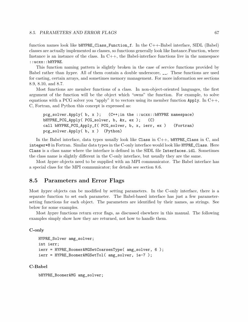
8.5. PARAMETERS AND ERROR FLAGS 67
function names look like bHYPRE_Class_Function_f. In the C++-Babel interface, SIDL (Babel)classes are actually implemented as classes, so functions generally look like Instance.Function, whereInstance is an instance of the class. In C++, the Babel-interface functions live in the namespace::ucxx::bHYPRE.
This function naming pattern is slightly broken in the case of service functions provided byBabel rather than hypre. All of them contain a double underscore, __. These functions are usedfor casting, certain arrays, and sometimes memory management. For more information see sections8.9, 8.10, and 8.7.
Most functions are member functions of a class. In non-object-oriented languages, the firstargument of the function will be the object which “owns” the function. For example, to solveequations with a PCG solver you “apply” it to vectors using its member function Apply. In C++,C, Fortran, and Python this concept is expressed as:
pcg_solver.Apply( b, x ); (C++;in the ::ucxx::bHYPRE namespace)bHYPRE_PCG_Apply( PCG_solver, b, &x, ex ); (C)call bHYPRE_PCG_Apply_f( PCG_solver, b, x, ierr, ex ) (Fortran)pcg_solver.Apply( b, x ) (Python)
In the Babel interface, data types usually look like Class in C++, bHYPRE_Class in C, andinteger*8 in Fortran. Similar data types in the C-only interface would look like HYPRE_Class. HereClass is a class name where the interface is defined in the SIDL file Interfaces.idl. Sometimesthe class name is slightly different in the C-only interface, but usually they are the same.
Most hypre objects need to be supplied with an MPI communicator. The Babel interface hasa special class for the MPI communicator; for details see section 8.6.
8.5 Parameters and Error Flags
Most hypre objects can be modified by setting parameters. In the C-only interface, there is aseparate function to set each parameter. The Babel-based interface has just a few parameter-setting functions for each object. The parameters are identified by their names, as strings. Seebelow for some examples.
Most hypre functions return error flags, as discussed elsewhere in this manual. The followingexamples simply show how they are returned, not how to handle them.
C-only
HYPRE_Solver amg_solver;int ierr;ierr = HYPRE_BoomerAMGSetCoarsenType( amg_solver, 6 );ierr = HYPRE_BoomerAMGSetTol( amg_solver, 1e-7 );
C-Babel
bHYPRE_BoomerAMG amg_solver;

68 CHAPTER 8. BABEL-BASED INTERFACES
int ierr;ierr = bHYPRE_BoomerAMG_SetIntParameter( amg_solver, "CoarsenType", 6, ex );ierr = bHYPRE_BoomerAMG_SetDoubleParameter( amg_solver,
"Tolerance", 1e-7, ex);
Fortran-Babel
integer*8 amg_solverinteger ierrcall bHYPRE_BoomerAMG_SetIntParameter_f(1 amg_solver, "CoarsenType", 6, ierr, ex )call bHYPRE_BoomerAMG_SetDoubleParameter_f(1 amg_solver, "Tolerance", tol, ierr, ex )
C++-Babel
using namespace ::ucxx::bHYPRE;BoomerAMG amg_solver;ierr = amg_solver.SetIntParameter( "CoarsenType", 6);ierr = amg_solver.SetDoubleParameter( "Tolerance", 1e-7);
Python-Babel
ierr = solver.SetIntParameter( "CoarsenType", 6 )ierr = solver.SetDoubleParameter( "Tolerance", 1e-7 )
8.6 MPI Communicator
In the C-only hypre interface, and most normal MPI usage, one often needs an MPI communicator oftype MPI_Comm. What an MPI_Comm really is depends on the language and the MPI implementation.
But the Babel interface is supposed to be fundamentally independent of languages and imple-mentations. So the MPI communicator is wrapped in a special bHYPRE_MPICommunicator object.This, not an MPI_Comm object, is what you pass to all the Babel-interface functions which needan MPI communicator. Thus the language dependence of MPI is isolated in the function whichcreates the bHYPRE_MPICommunicator object. Here are examples of how to use this function:
C-Babel
bHYPRE_MPICommunicator mpi_comm;MPI_Comm mpicommworld = MPI_COMM_WORLD;MPI_Comm * C_mpi_comm = &mpicommworld;mpi_comm = bHYPRE_MPICommunicator_CreateC( C_mpi_comm, ex );
...parcsr_A = bHYPRE_IJParCSRMatrix_Create( mpi_comm,... );

8.7. MEMORY MANAGEMENT 69
C++-Babel
using namespace ::ucxx::bHYPRE;MPICommunicator mpi_comm;MPI_Comm mpicommworld = MPI_COMM_WORLD;MPI_Comm * C_mpi_comm = &mpicommworld;mpi_comm = MPICommunicator::CreateC( C_mpi_comm );
...parcsr_A = IJParCSRMatrix::Create( mpi_comm,... );
Fortran-Babel
integer*8 mpi_comminteger*8 F_mpi_commF_mpi_comm = MPI_COMM_WORLDcall bHYPRE_MPICommunicator_CreateF_f(F_mpi_comm,mpi_comm,ex)
...call bHYPRE_IJParCSRMatrix_Create_f( mpi_comm, ... )
8.7 Memory Management
You will want to destroy whatever objects you create. In C and Fortran, you must do this explicitly.Through the Babel-based interface to hypre, there are two ways to create something: by calling aCreate function or by calling a cast function. You can destroy things with a Destroy or deleteReffunction. For every call of Create or cast there must be a call of Destroy or deleteRef. Here isan example in C:
b = bHYPRE_IJParCSRVector_Create( mpi_comm, ilower, iupper, ex );vb = bHYPRE_Vector__cast( b, ex );bHYPRE_Vector_deleteRef( vb, ex );bHYPRE_IJParCSRVector_deleteRef( b, ex );
Here it is in Fortran:
call bHYPRE_IJParCSRVector_Create_f( mpi_comm, ilower, iupper,1 b, ex )call bHYPRE_Vector__cast_f( b, vb, ex )call bHYPRE_IJParCSRVector_deleteRef_f( vb, ex )call bHYPRE_IJParCSRVector_deleteRef_f( b, ex )
What is actually going on here is memory management by reference counting. Babel reference-counts all its objects. Reference counting means that the object contains an integer which countsthe number of outside references to the object. Babel will bump up the reference count by onewhen you call a Create or cast function. Note that each of those functions normally is used to

70 CHAPTER 8. BABEL-BASED INTERFACES
assign an object to a variable. In C and Fortran it is up to you do decrement the reference countwhen that variable is no longer needed.
With Babel, reference counting is automatic in C++, so you will not normally need to do anymemory management yourself.
If you are interested in doing more with reference counting, see the Babel users’ manual for moreinformation. In some cases you may find Babel’s memory tools useful, e.g. if you copy pointers toBabel objects.
8.8 Casting
If your code is written in C or Fortran, you will occasionally need to call a Babel cast function.This section tells you why and how.
Functions are generally written in as much generality as possible. For example, the PCGalgorithm works the same for any kind of matrix and vector, as long as it can multiply a matrix andvector, compute an inner product, and so forth. So two of its arguments are of type bHYPRE_Vector.But when you create a vector you have to decide how it’s going to be stored! So you have to declareit as a more specific data type, e.g. bHYPRE_StructVector. To apply the PCG solver to that vectorin C or Fortran, you have to call a cast function to change its data type.
In C++ and Python, you do not normally need to call a cast function.Be careful to call a deleteRef or Destroy function to correspond to every cast function, as
discussed in section 8.7.Here are examples of casting in C and Fortran.
bHYPRE_StructVector b_S = bHYPRE_StructVector_Create(...);bHYPRE_Vector b = bHYPRE_Vector__cast( b_S, ex );hypre_Vector x;bHYPRE_PCG PCG_solver;bHYPRE_PCG_Apply( PCG_solver, b, &x, ex );bHYPRE_Vector_deleteRef( b, ex );bHYPRE_StructVector_deleteRef( b_S, ex );
integer*8 b_Sinteger*8 binteger*8 xinteger*8 PCG_solvercall bHYPRE_StructVector_Create_f(...,b_S, ex )call bHYPRE_Vector__cast_f( b_S, b, ex )call bHYPRE_PCG_Apply_f( PCG_solver, b, x, ierr, ex )call bHYPRE_Vector_deleteRef_f( b, ex )call bHYPRE_StructVector_deleteRef_f( b_S, ex )
(Other code not shown would set up the matrix, provide it and parameters to the solver, set upthe vectors, and so forth).

8.9. THE HYPRE OBJECT STRUCTURE 71
8.9 The HYPRE Object Structure
Even though it is written in C, hypre is object-oriented in its conceptual design. The objectstructure of hypre is often visible, for example in names of structs and functions. It is even morevisible in the Babel-based interface than in the C-only interface. In both interfaces, you can usehypre without any knowledge of its object structure or object-oriented programming. This sectionis for you if you have some basic knowledge of object-oriented concepts and if you are curious abouthow they appear in hypre.
In this section we will touch on some of the more notable features and peculiarities of the objectsystem as seen through the Babel-based interface. It is completely described elsewhere: the objectstructure is precisely defined in the a file Interfaces.idl, written in SIDL, which is short for“Scientific Interface Definition Language”. For more information about the SIDL language, visitthe Babel project website, http://www.llnl.gov/CASC/components. For the briefest possibledescription of the overall ideas of the hypre object system, see Figure 8.1.
Babel translates this object structure as appropriate for the language the user uses - fromSIDL’s interfaces and classes to C++ classes, or to mangled names in C and Fortran. For exam-ple the StructVector class defined in Interfaces.idl can appear as a C++ class also namedStructVector (in the bHYPRE namespace), as a C struct named bHYPRE_StructVector, or as aFortran integer*8. Its member function SetValues can appear in C++ as a member functionSetValues, in C as a function bHYPRE_StructVector_SetValues, or in Fortran as a subroutinebHYPRE_StructVector_SetValues_f.
The Babel interface goes beyond the hypre design in that a solver and matrix are both a kindof operator, i.e. something which acts on a vector to compute another vector. If a solver takes apreconditioner, it is called a preconditioned solver. There is no class or interface for preconditioners— it is possible, though not always wise, to use any solver as a preconditioner.
In order for a solver to act as an operator, to map a vector to a vector, it must contain notonly a solution method but also the equations to be solved. So you supply the solver with a matrixwhile constructing the solver.
All solvers have very similar interfaces, so most of their features are accessible through theircommon Solver interface. But each has its own peculiarities and each takes a different set ofparameters. Most solvers are specific to one or two matrix classes. An exception is the four Krylovsolvers, which will run with any matrix.
In contrast to the solvers, matrices have almost nothing in common other than being operators,i.e. a matrix can multiply a vector to compute another vector. Once the storage scheme of thematrix is specified there is much to do - such as specifying stencils, index ranges, and grids. Thereare four different classes of matrix for four different storage schemes - ParCSR, structured, andtwo kinds of semi-structured matrix. ParCSR matrices are generally used for unstructured meshesbut do not incorporate the mesh. A structured matrix includes a structured grid. The semistruc-tured matrix classes share the same interface with minimal modifications, and both contain meshinformation. But their implementations, e.g. matrix storage, are different.
Conceptually, there can be multiple views, or ways of interfacing, to a matrix. Or one type ofview can be used for more than one matrix class. At present, the Babel interface doesn’t contain
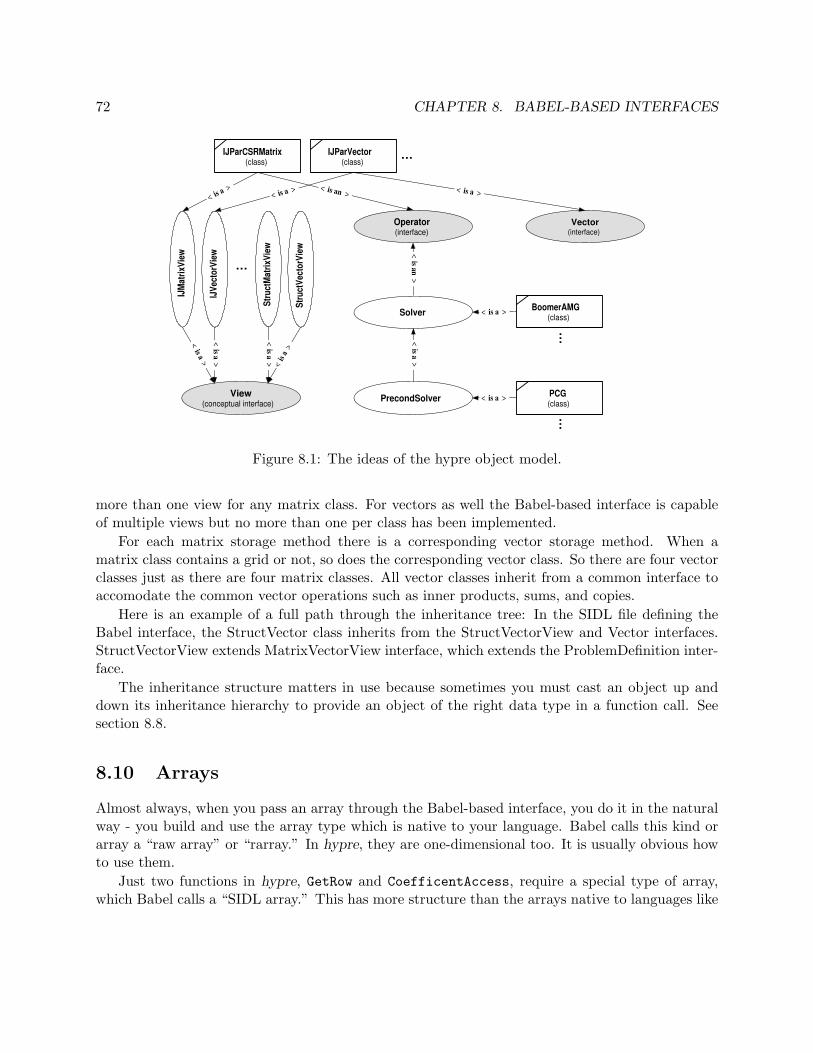
72 CHAPTER 8. BABEL-BASED INTERFACES
View (conceptual interface)
< is a >
IJM
atrix
View
IJVe
ctor
View
Stru
ctM
atrix
View
Stru
ctVe
ctor
View
…
< is a >
< is a > < is
a >
IJParCSRMatrix (class)
Operator (interface)
Solver
PrecondSolver < is an >
< is a >
Vector (interface)
< is a > < is an >
IJParVector (class)
< is a > < is a >
PCG (class)
< is a >
< is a >
BoomerAMG (class)
…
…
…
Figure 8.1: The ideas of the hypre object model.
more than one view for any matrix class. For vectors as well the Babel-based interface is capableof multiple views but no more than one per class has been implemented.
For each matrix storage method there is a corresponding vector storage method. When amatrix class contains a grid or not, so does the corresponding vector class. So there are four vectorclasses just as there are four matrix classes. All vector classes inherit from a common interface toaccomodate the common vector operations such as inner products, sums, and copies.
Here is an example of a full path through the inheritance tree: In the SIDL file defining theBabel interface, the StructVector class inherits from the StructVectorView and Vector interfaces.StructVectorView extends MatrixVectorView interface, which extends the ProblemDefinition inter-face.
The inheritance structure matters in use because sometimes you must cast an object up anddown its inheritance hierarchy to provide an object of the right data type in a function call. Seesection 8.8.
8.10 Arrays
Almost always, when you pass an array through the Babel-based interface, you do it in the naturalway - you build and use the array type which is native to your language. Babel calls this kind orarray a “raw array” or “rarray.” In hypre, they are one-dimensional too. It is usually obvious howto use them.
Just two functions in hypre, GetRow and CoefficentAccess, require a special type of array,which Babel calls a “SIDL array.” This has more structure than the arrays native to languages like

8.11. BUILDING HYPRE WITH THE BABEL INTERFACE 73
C or Fortran - it accomodates reference counting and knows its own size, for example.The following examples show a way to declare, read, and destroy a SIDL array. The GetRow
and CoefficentAccess functions create their output arrays, so there is no need to create your own.For more information on these arrays, read the Babel documentation at http://www.llnl.gov/CASC/components.
C
struct sidl_int__array *row_js;struct sidl_double__array *row_data;bHYPRE_IJParCSRMatrix_GetRow( A, i, &row_size, &row_js, &row_data, ex );for ( k=0; k<row_size; ++k )
col[k] = sidl_int__array_get1( row_js, k );data[k] = sidl_double__array_get1( row_data, k );
sidl_int__array_deleteRef( row_j, ex );sidl_double__array_deleteRef( row_data, ex );
Fortran
integer*8 row_js;integer*8 row_data;call bHYPRE_IJParCSRMatrix_GetRow_f( A, i, row_size, row_js,1 row_data, ex )do k = 1, row_size
call sidl_int__array_get1_f( row_js, k-1, col(k) )call sidl_double__array_get1_f( row_data, k-1, data(k) )
enddocall sidl_int__array_deleteRef( row_j, ex )call sidl_double__array_deleteRef( row_data, ex )
8.11 Building HYPRE with the Babel Interface
You can build hypre almost the same way with and without the Babel-based interface. Normallythe only difference is that the configure line needs an extra argument; for example:
configure --with-babelmake
rather than
configuremake

74 CHAPTER 8. BABEL-BASED INTERFACES
The configure system will enable whatever built-in languages it can find compilers for.The configure system for the runtime portion of Babel (included with hypre and enabled with
the Babel-based interface) will automatically compile and run a few tiny test programs. This hasbeen a problem in multiprocessing AIX systems, where compiled programs are normally run in adifferent environment from the configure system. For AIX systems with POE, the hypre distributionincludes a workaround script, nopoe. When necessary, build hypre as follows instead of the above:
nopoe configure --with-babelmake
8.11.1 Building HYPRE with Python Using the Babel Interface
To build the hypre library so you can call it from Python code, the first step is to build a suitablePython! Start with a recent version of Python with the Numeric Python extension; for details seethe section on recommended external software in the Babel Users’ Manual.
We have only tested hypre’s Python interface with pyMPI, a Python extension which supportsMPI. It is likely that you can make it work with other MPI extensions, or even no MPI at all. Ifyou try this, let us know how it works.
You will need write access to your Python’s site-packages directory. When you install pyMPIit creates another instance of Python, so this should not be a problem.
You must configure and build hypre with shared libraries, because Python requires them. Andspecify what Python you are building for; files will be written into its site-packages directory. Forexample:
configure --with-babel --enable-shared --enable-python=pyMPImake
Finally, you need to set two environment variables. LD_LIBRARY_PATH must include the path tothe hypre shared libraries, e.g. src/hypre/lib. SIDL_DLL_PATH must include the path to an .sclfile generated for the Python interface, e.g.
src/babel/bHYPREClient-P/libbHYPRE.scl
If you are running multiple processes, these environment variables may need to be set in a dotfileso all processes will use the same values.
See the examples directory for an example of how to write a Python program which uses hypre.

Bibliography
[1] S. F. Ashby and R. D. Falgout. A parallel multigrid preconditioned conjugate gradient al-gorithm for groundwater flow simulations. Nuclear Science and Engineering, 124(1):145–159,September 1996. Also available as LLNL Technical Report UCRL-JC-122359. 38
[2] A.H. Baker, R.D. Falgout, and U.M. Yang. An assumed partition algorithm for determiningprocessor inter-communication. Parallel Computing, 32:394–414, 2006. 34
[3] P. N. Brown, R. D. Falgout, and J. E. Jones. Semicoarsening multigrid on distributed memorymachines. SIAM J. Sci. Comput., 21(5):1823–1834, 2000. Special issue on the Fifth CopperMountain Conference on Iterative Methods. Also available as LLNL technical report UCRL-JC-130720. 37
[4] E. Chow. A priori sparsity patterns for parallel sparse approximate inverse preconditioners.SIAM J. Sci. Comput., 21:1804–1822, 2000. 48
[5] H. De Sterck, U. M. Yang, and J. Heys. Reducing complexity in parallel algebraic multigridpreconditioners. SIAM Journal on Matrix Analysis and Applications, 27:1019–1039, 2006. Alsoavailable as LLNL technical report UCRL-JRNL-206780. 42
[6] R. L. Clay et al. An annotated reference guide to the Finite Element Interface (FEI) specifica-tion, Version 1.0. Technical Report SAND99-8229, Sandia National Laboratories, Livermore,CA, 1999. 27
[7] R. D. Falgout and J. E. Jones. Multigrid on massively parallel architectures. In E. Dick,K. Riemslagh, and J. Vierendeels, editors, Multigrid Methods VI, volume 14 of Lecture Notesin Computational Science and Engineering, pages 101–107, Berlin, 2000. Springer. Proc. ofthe Sixth European Multigrid Conference held in Gent, Belgium, September 27-30, 1999. Alsoavailable as LLNL technical report UCRL-JC-133948. 37, 38
[8] V. E. Henson and U. M. Yang. BoomerAMG: a parallel algebraic multigrid solver and pre-conditioner. Applied Numerical Mathematics, 41(5):155–177, 2002. Also available as LLNLtechnical report UCRL-JC-141495. 41
[9] R. Hiptmair and J. Xu. Nodal auxiliary space preconditioning in H(curl) and H(div) spaces.Numer. Math., 2006. to appear. 43
75

76 BIBLIOGRAPHY
[10] D. Hysom and A. Pothen. Efficient parallel computation of ILU(k) preconditioners. In Pro-ceedings of Supercomputing ’99. ACM, November 1999. Published on CDROM, ISBN #1-58113-091-0, ACM Order #415990, IEEE Computer Society Press Order # RS00197. 49
[11] D. Hysom and A. Pothen. A scalable parallel algorithm for incomplete factor preconditioning.SIAM J. Sci. Comput., 22(6):2194–2215, 2001. 49
[12] J. Jones and B. Lee. A multigrid method for variable coefficient maxwell’s equations. SIAMJ. Sci. Comput., 27:1689–1708, 2006. 40
[13] G. Karypis and V. Kumar. Parallel threshold-based ILU factorization. Technical Report061, University of Minnesota, Department of Computer Science/Army HPC Research Center,Minneapolis, MN 5455, 1998. 53
[14] Tz. V. Kolev and P. S. Vassilevski. Parallel H1-based auxiliary space AMG solver for H(curl)problems. Technical Report UCRL-TR-222763, LLNL, 2006. 43
[15] Tz. V. Kolev and P. S. Vassilevski. Some experience with a H1–based auxiliary space AMGfor H(curl)–problems. Technical Report UCRL-TR-221841, LLNL, 2006. 43
[16] S. F. McCormick. Multilevel Adaptive Methods for Partial Differential Equations, volume 6 ofFrontiers in Applied Mathematics. SIAM Books, Philadelphia, 1989. 22, 38
[17] J.E. Morel, Randy M. Roberts, and Mikhail J. Shashkov. A local support-operators diffusiondiscretization scheme for quadrilateral r-z meshes. J. Comp. Physics, 144:17–51, 1998. 18
[18] J. W. Ruge and K. Stuben. Algebraic multigrid (AMG). In S. F. McCormick, editor, MultigridMethods, volume 3 of Frontiers in Applied Mathematics, pages 73–130. SIAM, Philadelphia,PA, 1987. 41, 42
[19] S. Schaffer. A semi-coarsening multigrid method for elliptic partial differential equations withhighly discontinuous and anisotropic coefficients. SIAM J. Sci. Comput., 20(1):228–242, 1998.37
[20] K. Stuben. Algebraic multigrid (AMG): an introduction with applications. In U. Trottenberg,C. Oosterlee, and A. Schuller, editors, Multigrid. Academic Press, 2001. 42
[21] P. Vanek, M. Brezina, and J. Mandel. Convergence of algebraic multigrid based on smoothedaggregation. Numerische Mathematik, 88:559–579, 2001. 47
[22] P. Vanek, J. Mandel, and M. Brezina. Algebraic multigrid based on smoothed aggregation forsecond and fourth order problems. Computing, 56:179–196, 1996. 47
[23] U. M. Yang. On the use of relaxation parameters in hybrid smoothers. Numerical LinearAlgebra with Applications, 11:155–172, 2004. 42

BIBLIOGRAPHY 77
[24] U. M. Yang. Parallel algebraic multigrid methods - high performance preconditioners. InA. M. Bruaset and A. Tveito, editors, Numerical Solution of Partial Differential Equations onParallel Computers, pages 209–236. Springer-Verlag, 2006. Also available as LLNL technicalreport UCRL-BOOK-208032. 41