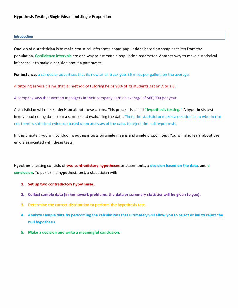
Hypothesis Testing: Single Mean and Single Proportion

Introduction

One job of a statistician is to make statistical inferences about populations based on samples taken from the

population. Confidence intervals are one way to estimate a population parameter. Another way to make a statistical

inference is to make a decision about a parameter.

For instance, a car dealer advertises that its new small truck gets 35 miles per gallon, on the average.

A tutoring service claims that its method of tutoring helps 90% of its students get an A or a B.

A company says that women managers in their company earn an average of $60,000 per year.

A statistician will make a decision about these claims. This process is called "hypothesis testing." A hypothesis test

involves collecting data from a sample and evaluating the data. Then, the statistician makes a decision as to whether or

not there is sufficient evidence based upon analyses of the data, to reject the null hypothesis.

In this chapter, you will conduct hypothesis tests on single means and single proportions. You will also learn about the

errors associated with these tests.

Hypothesis testing consists of two contradictory hypotheses or statements, a decision based on the data, and a

conclusion. To perform a hypothesis test, a statistician will:

1. Set up two contradictory hypotheses.

2. Collect sample data (in homework problems, the data or summary statistics will be given to you).

3. Determine the correct distribution to perform the hypothesis test.

4. Analyze sample data by performing the calculations that ultimately will allow you to reject or fail to reject the

null hypothesis.

5. Make a decision and write a meaningful conclusion.

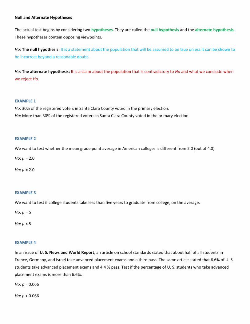
Null and Alternate Hypotheses

The actual test begins by considering two hypotheses. They are called the null hypothesis and the alternate hypothesis.

These hypotheses contain opposing viewpoints.

Ho: The null hypothesis: It is a statement about the population that will be assumed to be true unless it can be shown to

be incorrect beyond a reasonable doubt.

Ha: The alternate hypothesis: It is a claim about the population that is contradictory to Ho and what we conclude when

we reject Ho.

EXAMPLE 1

Ho: 30% of the registered voters in Santa Clara County voted in the primary election.

Ha: More than 30% of the registered voters in Santa Clara County voted in the primary election.

EXAMPLE 2

We want to test whether the mean grade point average in American colleges is different from 2.0 (out of 4.0).

Ho: μ = 2.0

Ha: μ ≠ 2.0

EXAMPLE 3

We want to test if college students take less than five years to graduate from college, on the average.

Ho: μ = 5

Ha: μ < 5

EXAMPLE 4

In an issue of U. S. News and World Report, an article on school standards stated that about half of all students in

France, Germany, and Israel take advanced placement exams and a third pass. The same article stated that 6.6% of U. S.

students take advanced placement exams and 4.4 % pass. Test if the percentage of U. S. students who take advanced

placement exams is more than 6.6%.

Ho: p = 0.066

Ha: p > 0.066

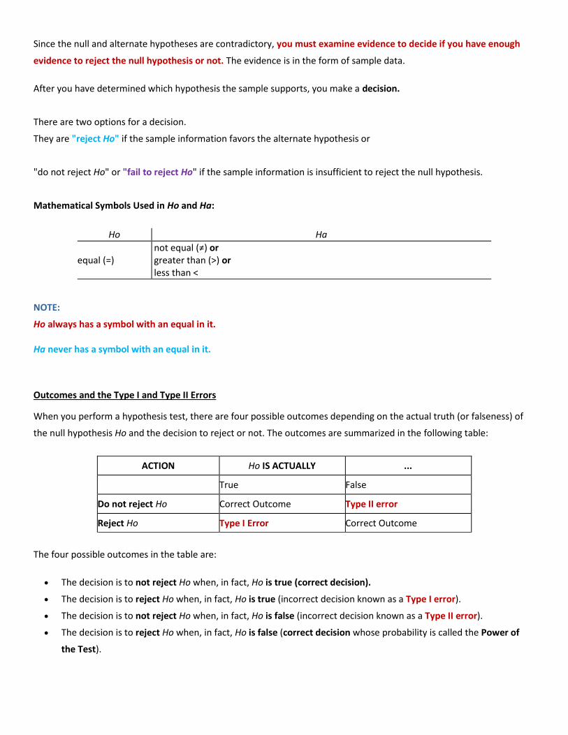
Since the null and alternate hypotheses are contradictory, you must examine evidence to decide if you have enough

evidence to reject the null hypothesis or not. The evidence is in the form of sample data.

After you have determined which hypothesis the sample supports, you make a decision.

There are two options for a decision.

They are "reject Ho" if the sample information favors the alternate hypothesis or

"do not reject Ho" or "fail to reject Ho" if the sample information is insufficient to reject the null hypothesis.

Mathematical Symbols Used in Ho and Ha:

Ho Ha

equal (=) not equal (≠) or greater than (>) or less than <

NOTE:

Ho always has a symbol with an equal in it.

Ha never has a symbol with an equal in it.

Outcomes and the Type I and Type II Errors

When you perform a hypothesis test, there are four possible outcomes depending on the actual truth (or falseness) of

the null hypothesis Ho and the decision to reject or not. The outcomes are summarized in the following table:

ACTION Ho IS ACTUALLY ...

True False

Do not reject Ho Correct Outcome Type II error

Reject Ho Type I Error Correct Outcome

The four possible outcomes in the table are:

The decision is to not reject Ho when, in fact, Ho is true (correct decision).

The decision is to reject Ho when, in fact, Ho is true (incorrect decision known as a Type I error).

The decision is to not reject Ho when, in fact, Ho is false (incorrect decision known as a Type II error).

The decision is to reject Ho when, in fact, Ho is false (correct decision whose probability is called the Power of

the Test).

Each of the errors occurs with a particular probability. The Greek letters α and β represent the probabilities.

α = probability of a Type I error = P(Type I error) = probability of rejecting the null hypothesis when the null hypothesis is

true.

β = probability of a Type II error = P(Type II error) = probability of not rejecting the null hypothesis when the null

hypothesis is false.

α and β should be as small as possible because they are probabilities of errors. They are rarely 0.

The Power of the Test is 1−β. Ideally, we want a high power that is as close to 1 as possible. Increasing the sample size

can increase the Power of the Test.

The following are examples of Type I and Type II errors.

EXAMPLE 1

Suppose the null hypothesis, Ho, is: Frank's rock climbing equipment is safe.

Type I error: Frank thinks that his rock climbing equipment may not be safe when, in fact, it really is safe.

Type II error: Frank thinks that his rock climbing equipment may be safe when, in fact, it is not safe.

α = probability that Frank thinks his rock climbing equipment may not be safe when, in fact, it really is safe.

β = probability that Frank thinks his rock climbing equipment may be safe when, in fact, it is not safe.

Notice that, in this case, the error with the greater consequence is the Type II error. (If Frank thinks his rock climbing

equipment is safe, he will go ahead and use it.)

EXAMPLE 2

Suppose the null hypothesis, Ho, is: The victim of an automobile accident is alive when he arrives at the emergency

room of a hospital.

Type I error: The emergency crew thinks that the victim is dead when, in fact, the victim is alive.

Type II error: The emergency crew does not know if the victim is alive when, in fact, the victim is dead.

α = probability that the emergency crew thinks the victim is dead when, in fact, he is really alive = P(Type I error).

β = probability that the emergency crew does not know if the victim is alive when, in fact, the victim is dead = P(Type II

error).

The error with the greater consequence is the Type I error. (If the emergency crew thinks the victim is dead, they will not

treat him.)

Distribution Needed for Hypothesis Testing

Earlier in the course, we discussed sampling distributions.

Particular distributions are associated with hypothesis testing.

Perform tests of a population mean using a normal distribution or a student's-t distribution. (Remember, use a

student's-t distribution when the population standard deviation is unknown and the distribution of the sample mean is

approximately normal.)

In this chapter we perform tests of a population proportion using a normal distribution (usually n is large or the sample

size is large).

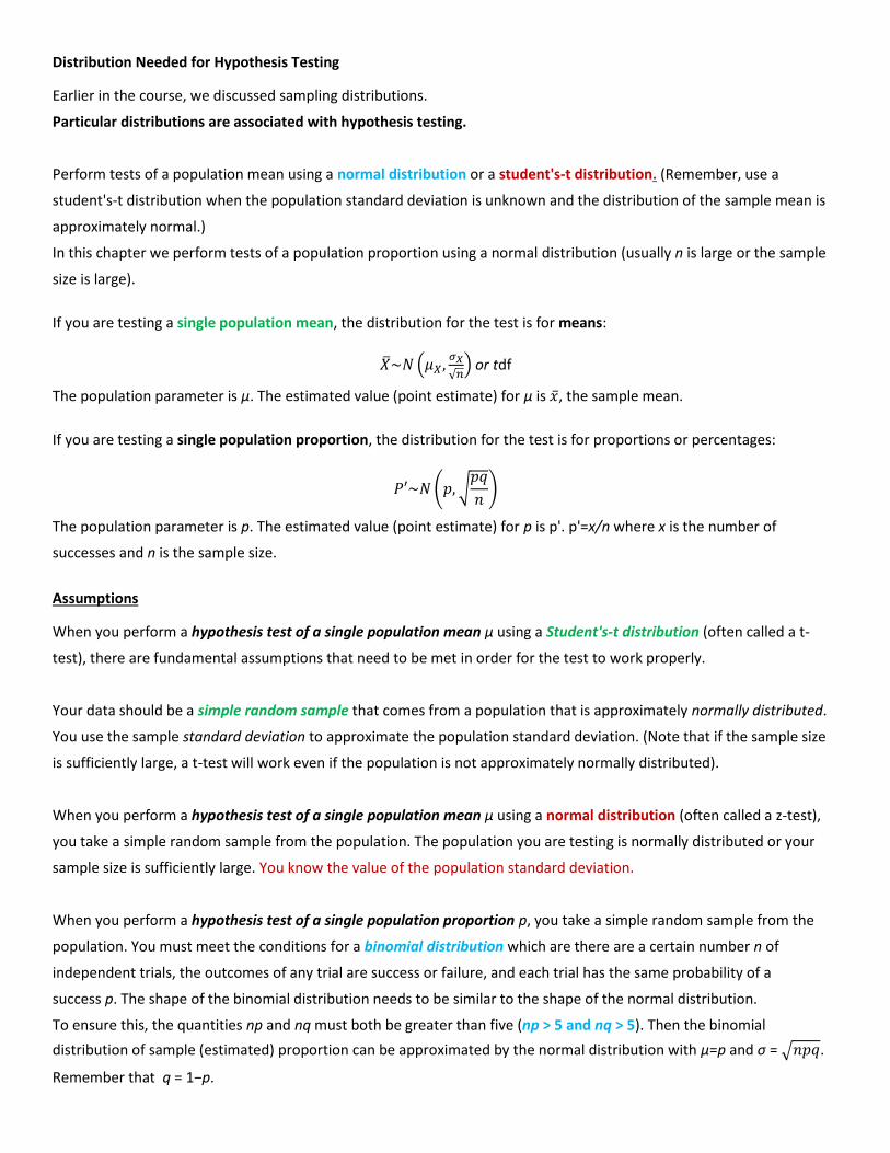
If you are testing a single population mean, the distribution for the test is for means:

(

√ ) or tdf

The population parameter is μ. The estimated value (point estimate) for μ is , the sample mean.

If you are testing a single population proportion, the distribution for the test is for proportions or percentages:

( √

)

The population parameter is p. The estimated value (point estimate) for p is p'. p'=x/n where x is the number of

successes and n is the sample size.

Assumptions

When you perform a hypothesis test of a single population mean μ using a Student's-t distribution (often called a t-

test), there are fundamental assumptions that need to be met in order for the test to work properly.

Your data should be a simple random sample that comes from a population that is approximately normally distributed.

You use the sample standard deviation to approximate the population standard deviation. (Note that if the sample size

is sufficiently large, a t-test will work even if the population is not approximately normally distributed).

When you perform a hypothesis test of a single population mean μ using a normal distribution (often called a z-test),

you take a simple random sample from the population. The population you are testing is normally distributed or your

sample size is sufficiently large. You know the value of the population standard deviation.

When you perform a hypothesis test of a single population proportion p, you take a simple random sample from the

population. You must meet the conditions for a binomial distribution which are there are a certain number n of

independent trials, the outcomes of any trial are success or failure, and each trial has the same probability of a

success p. The shape of the binomial distribution needs to be similar to the shape of the normal distribution.

To ensure this, the quantities np and nq must both be greater than five (np > 5 and nq > 5). Then the binomial

distribution of sample (estimated) proportion can be approximated by the normal distribution with μ=p and σ = √ .

Remember that q = 1−p.

Using the Sample to Test the Null Hypothesis

Use the sample data to calculate the actual probability of getting the test result, called the p-value. The p-value is

the probability that, if the null hypothesis is true, the results from another randomly selected sample will be as

extreme or more extreme as the results obtained from the given sample.

A large p-value calculated from the data indicates that we should fail to reject the null hypothesis.

A small p-value, shows it is unlikely to get this outcome, and there is strong evidence against the null hypothesis. We

would reject the null hypothesis if the evidence is strongly against it.

Draw a graph that shows the p-value. The hypothesis test is easier to perform if you use a graph because you see the

problem more clearly.

EXAMPLE 1: (to illustrate the p-value)

Suppose a baker claims that his bread height is more than 15 cm, on the average. Several of his customers do not

believe him. To persuade his customers that he is right, the baker decides to do a hypothesis test. He bakes 10 loaves of

bread. The mean height of the sample loaves is 17 cm. The baker knows from baking hundreds of loaves of bread that

the standard deviation for the height is 0.5 cm. and the distribution of heights is normal.

The null hypothesis could be Ho: μ = 15

The alternate hypothesis is Ha: μ > 15

Since σ is known (σ = 0.5 cm.), the distribution for the population is known to be normal with mean μ = 15 and standard

deviation

√

√

Suppose the null hypothesis is true (the mean height of the loaves is no more than 15 cm).

Then is the mean height (17 cm) calculated from the sample unexpectedly large?

The hypothesis test works by asking the question how unlikely the sample mean would be if the null hypothesis were

true.

The graph shows how far out the sample mean is on the normal curve. The p-value is the probability that, if we were to

take other samples, any other sample mean would fall at least as far out as 17 cm.

The p-value, then, is the probability that a sample mean is the same or greater than 17 cm. when the population

mean is, in fact, 15 cm.

We can calculate this probability using the normal distribution for means from Chapter 7.

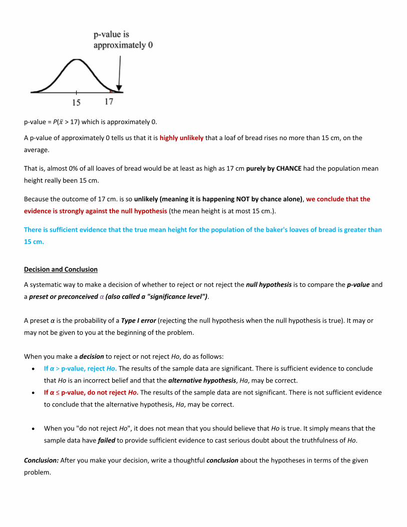
p-value = P( > 17) which is approximately 0.

A p-value of approximately 0 tells us that it is highly unlikely that a loaf of bread rises no more than 15 cm, on the

average.

That is, almost 0% of all loaves of bread would be at least as high as 17 cm purely by CHANCE had the population mean

height really been 15 cm.

Because the outcome of 17 cm. is so unlikely (meaning it is happening NOT by chance alone), we conclude that the

evidence is strongly against the null hypothesis (the mean height is at most 15 cm.).

There is sufficient evidence that the true mean height for the population of the baker's loaves of bread is greater than

15 cm.

Decision and Conclusion

A systematic way to make a decision of whether to reject or not reject the null hypothesis is to compare the p-value and

a preset or preconceived α (also called a "significance level").

A preset α is the probability of a Type I error (rejecting the null hypothesis when the null hypothesis is true). It may or

may not be given to you at the beginning of the problem.

When you make a decision to reject or not reject Ho, do as follows:

If α > p-value, reject Ho. The results of the sample data are significant. There is sufficient evidence to conclude

that Ho is an incorrect belief and that the alternative hypothesis, Ha, may be correct.

If α ≤ p-value, do not reject Ho. The results of the sample data are not significant. There is not sufficient evidence

to conclude that the alternative hypothesis, Ha, may be correct.

When you "do not reject Ho", it does not mean that you should believe that Ho is true. It simply means that the

sample data have failed to provide sufficient evidence to cast serious doubt about the truthfulness of Ho.

Conclusion: After you make your decision, write a thoughtful conclusion about the hypotheses in terms of the given

problem.

Additional Information

In a hypothesis test problem, you may see words such as "the level of significance is 1%." The "1%" is the

preconceived or preset α.

The statistician setting up the hypothesis test selects the value of α to use before collecting the sample data.

If no level of significance is given, the accepted standard is to use α = 0.05.

When you calculate the p-value and draw the picture, the p-value is the area in the left tail, the right tail, or split

evenly between the two tails. For this reason, we call the hypothesis test left, right, or two tailed.

The alternate hypothesis, Ha, tells you if the test is left, right, or two-tailed. It is the key to conducting the

appropriate test.

Ha never has a symbol that contains an equal sign.

Thinking about the meaning of the p-value: A data analyst (and anyone else) should have more confidence that

he made the correct decision to reject the null hypothesis with a smaller p-value (for example, 0.001 as opposed

to 0.04) even if using the 0.05 level for alpha.

Similarly, for a large p-value like 0.4, as opposed to a p-value of 0.056 (alpha = 0.05 is less than either number), a

data analyst should have more confidence that she made the correct decision in failing to reject the null

hypothesis. This makes the data analyst use judgment rather than mindlessly applying rules.

The following examples illustrate a left, right, and two-tailed test.

EXAMPLE 1

Ho: μ = 5 Ha: μ < 5

Test of a single population mean. Ha tells you the test is left-tailed. The picture of the p-value is as follows:

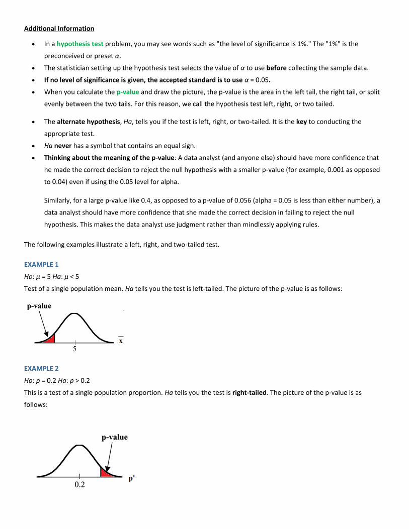
EXAMPLE 2

Ho: p = 0.2 Ha: p > 0.2

This is a test of a single population proportion. Ha tells you the test is right-tailed. The picture of the p-value is as

follows:

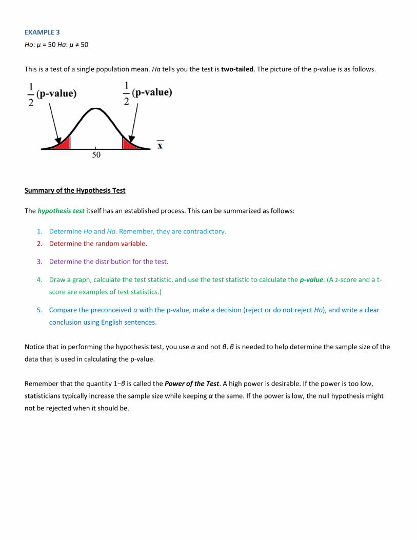
EXAMPLE 3

Ho: μ = 50 Ha: μ ≠ 50

This is a test of a single population mean. Ha tells you the test is two-tailed. The picture of the p-value is as follows.

Summary of the Hypothesis Test

The hypothesis test itself has an established process. This can be summarized as follows:

1. Determine Ho and Ha. Remember, they are contradictory.

2. Determine the random variable.

3. Determine the distribution for the test.

4. Draw a graph, calculate the test statistic, and use the test statistic to calculate the p-value. (A z-score and a t-

score are examples of test statistics.)

5. Compare the preconceived α with the p-value, make a decision (reject or do not reject Ho), and write a clear

conclusion using English sentences.

Notice that in performing the hypothesis test, you use α and not β. β is needed to help determine the sample size of the

data that is used in calculating the p-value.

Remember that the quantity 1−β is called the Power of the Test. A high power is desirable. If the power is too low,

statisticians typically increase the sample size while keeping α the same. If the power is low, the null hypothesis might

not be rejected when it should be.

Examples

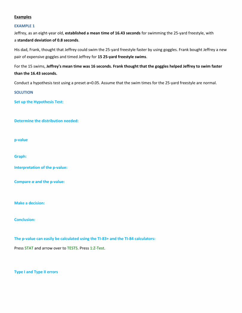
EXAMPLE 1

Jeffrey, as an eight-year old, established a mean time of 16.43 seconds for swimming the 25-yard freestyle, with

a standard deviation of 0.8 seconds.

His dad, Frank, thought that Jeffrey could swim the 25-yard freestyle faster by using goggles. Frank bought Jeffrey a new

pair of expensive goggles and timed Jeffrey for 15 25-yard freestyle swims.

For the 15 swims, Jeffrey's mean time was 16 seconds. Frank thought that the goggles helped Jeffrey to swim faster

than the 16.43 seconds.

Conduct a hypothesis test using a preset α=0.05. Assume that the swim times for the 25-yard freestyle are normal.

SOLUTION

Set up the Hypothesis Test:

Determine the distribution needed:

p-value

Graph:

Interpretation of the p-value:

Compare α and the p-value:

Make a decision:

Conclusion:

The p-value can easily be calculated using the TI-83+ and the TI-84 calculators:

Press STAT and arrow over to TESTS. Press 1:Z-Test.

Type I and Type II errors

EXAMPLE 2

A college football coach thought that his players could bench press a mean weight of 275 pounds. It is known that

the standard deviation is 55 pounds. Three of his players thought that the mean weight was more than that amount.

They asked 30 of their teammates for their estimated maximum lift on the bench press exercise. The data ranged from

205 pounds to 385 pounds. The actual different weights were (frequencies are in parentheses):

205(3); 215(3); 225(1); 241(2); 252(2); 265(2); 275(2); 313(2); 316(5); 338(2); 341(1); 345(2); 368(2); 385(1).

(Source: data from Reuben Davis, Kraig Evans, and Scott Gunderson.)

Conduct a hypothesis test using a 2.5% level of significance to determine if the bench press mean is more than 275

pounds.

Set up the Hypothesis Test:

Determine the distribution needed:

p-value

Graph:

Interpretation of the p-value:

Compare α and the p-value:

Make a decision:

Conclusion:

The p-value can easily be calculated using the TI-83+ and the TI-84 calculators:

Press STAT and arrow over to TESTS. Press 1:Z-Test.

Type I and Type II errors

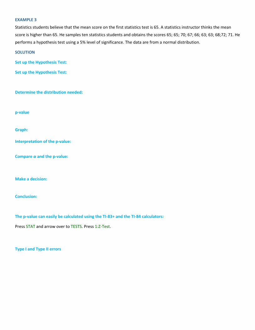
EXAMPLE 3

Statistics students believe that the mean score on the first statistics test is 65. A statistics instructor thinks the mean

score is higher than 65. He samples ten statistics students and obtains the scores 65; 65; 70; 67; 66; 63; 63; 68;72; 71. He

performs a hypothesis test using a 5% level of significance. The data are from a normal distribution.

SOLUTION

Set up the Hypothesis Test:

Set up the Hypothesis Test:

Determine the distribution needed:

p-value

Graph:

Interpretation of the p-value:

Compare α and the p-value:

Make a decision:

Conclusion:

The p-value can easily be calculated using the TI-83+ and the TI-84 calculators:

Press STAT and arrow over to TESTS. Press 1:Z-Test.

Type I and Type II errors

EXAMPLE 4

Joon believes that 50% of first-time brides in the United States are younger than their grooms. She performs a

hypothesis test to determine if the percentage is the same or different from 50%. Joon samples 100 first-time

brides and 53 reply that they are younger than their grooms. For the hypothesis test, she uses a 1% level of significance.

SOLUTION

Set up the Hypothesis Test:

Determine the distribution needed:

p-value

Graph:

Interpretation of the p-value:

Compare α and the p-value:

Make a decision:

Conclusion:

The p-value can easily be calculated using the TI-83+ and the TI-84 calculators:

Press STAT and arrow over to TESTS. Press 1:Z-Test.

Type I and Type II errors

EXAMPLE 5

A cell phone company has reason to believe that the proportion of households that have three cell phones is 30%.

Before they start a big advertising campaign, they conduct a hypothesis test. Their marketing people survey 150

households with the result that 43 of the households have three cell phones.

SOLUTION

Set up the Hypothesis Test:

Determine the distribution needed:

p-value

Graph:

Interpretation of the p-value:

Compare α and the p-value:

Make a decision:

Conclusion:

The p-value can easily be calculated using the TI-83+ and the TI-84 calculators:

Press STAT and arrow over to TESTS. Press 1:Z-Test.

Type I and Type II errors

Hypothesis Testing: Two Population Means and Two Population Proportions

Introduction

Studies often compare two groups. For example, researchers are interested in the effect aspirin has in preventing heart

attacks. Over the last few years, newspapers and magazines have reported about various aspirin studies involving two

groups. Typically, one group is given aspirin and the other group is given a placebo. Then, the heart attack rate is studied

over several years.

There are other situations that deal with the comparison of two groups. For example, studies compare various diet and

exercise programs. Politicians compare the proportion of individuals from different income brackets who might vote for

them. Students are interested in whether SAT or GRE preparatory courses really help raise their scores.

In the previous chapter, you learned to conduct hypothesis tests on single means and single proportions. You will

expand upon that in this chapter. You will compare two means or two proportions to each other. The general

procedure is still the same, just expanded.

To compare two means or two proportions, you work with two groups. The groups are classified either

as independent or matched pairs.

Independent groups mean that the two samples taken are independent, that is, sample values selected from one

population are not related in any way to sample values selected from the other population.

Matched pairs consist of two samples that are dependent. The parameter tested using matched pairs is the population

mean. The parameters tested using independent groups are either population means or population proportions.

This chapter deals with the following hypothesis tests:

Independent groups (samples are independent)

Test of two population means.

Test of two population proportions.

Matched or paired samples (samples are dependent)

Becomes a test of one population mean.

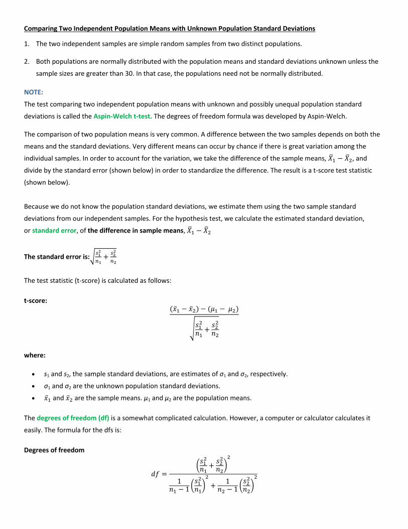
Comparing Two Independent Population Means with Unknown Population Standard Deviations

1. The two independent samples are simple random samples from two distinct populations.

2. Both populations are normally distributed with the population means and standard deviations unknown unless the

sample sizes are greater than 30. In that case, the populations need not be normally distributed.

NOTE:

The test comparing two independent population means with unknown and possibly unequal population standard

deviations is called the Aspin-Welch t-test. The degrees of freedom formula was developed by Aspin-Welch.

The comparison of two population means is very common. A difference between the two samples depends on both the

means and the standard deviations. Very different means can occur by chance if there is great variation among the

individual samples. In order to account for the variation, we take the difference of the sample means, , and

divide by the standard error (shown below) in order to standardize the difference. The result is a t-score test statistic

(shown below).

Because we do not know the population standard deviations, we estimate them using the two sample standard

deviations from our independent samples. For the hypothesis test, we calculate the estimated standard deviation,

or standard error, of the difference in sample means,

The standard error is:√

The test statistic (t-score) is calculated as follows:

t-score:

√

where:

s1 and s2, the sample standard deviations, are estimates of σ1 and σ2, respectively.

σ1 and σ2 are the unknown population standard deviations.

and are the sample means. μ1 and μ2 are the population means.

The degrees of freedom (df) is a somewhat complicated calculation. However, a computer or calculator calculates it

easily. The formula for the dfs is:

Degrees of freedom

(

)

(

)

(

)

When both sample sizes n1 and n2 are five or larger, the student's-t approximation is very good. Notice that the sample

variances (s1)2 and (s2)

2 are not pooled. (If the question comes up, do not pool the variances.)

NOTE: It is not necessary to compute this by hand. A calculator or computer easily computes it.

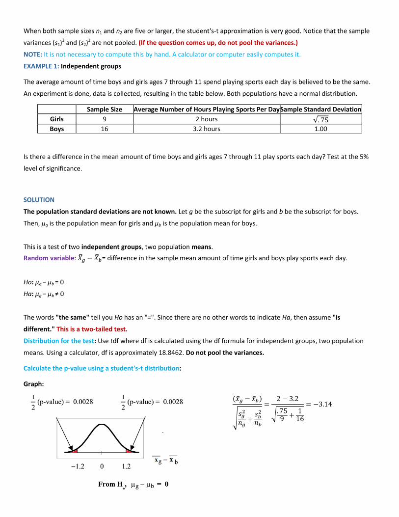
EXAMPLE 1: Independent groups

The average amount of time boys and girls ages 7 through 11 spend playing sports each day is believed to be the same.

An experiment is done, data is collected, resulting in the table below. Both populations have a normal distribution.

Sample Size Average Number of Hours Playing Sports Per Day Sample Standard Deviation

Girls 9 2 hours √ Boys 16 3.2 hours 1.00

Is there a difference in the mean amount of time boys and girls ages 7 through 11 play sports each day? Test at the 5%

level of significance.

SOLUTION

The population standard deviations are not known. Let g be the subscript for girls and b be the subscript for boys.

Then, μg is the population mean for girls and μb is the population mean for boys.

This is a test of two independent groups, two population means.

Random variable: = difference in the sample mean amount of time girls and boys play sports each day.

Ho: μg − μb = 0

Ha: μg − μb ≠ 0

The words "the same" tell you Ho has an "=". Since there are no other words to indicate Ha, then assume "is

different." This is a two-tailed test.

Distribution for the test: Use tdf where df is calculated using the df formula for independent groups, two population

means. Using a calculator, df is approximately 18.8462. Do not pool the variances.

Calculate the p-value using a student's-t distribution:

Graph:

√

√

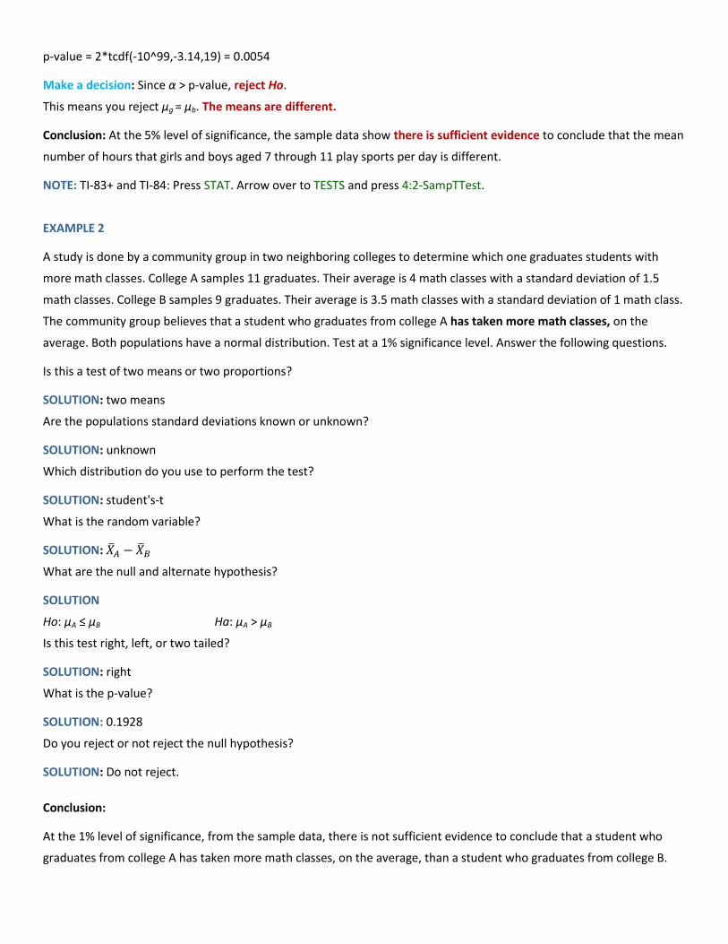
p-value = 2*tcdf(-10^99,-3.14,19) = 0.0054

Make a decision: Since α > p-value, reject Ho.

This means you reject μg = μb. The means are different.

Conclusion: At the 5% level of significance, the sample data show there is sufficient evidence to conclude that the mean

number of hours that girls and boys aged 7 through 11 play sports per day is different.

NOTE: TI-83+ and TI-84: Press STAT. Arrow over to TESTS and press 4:2-SampTTest.

EXAMPLE 2

A study is done by a community group in two neighboring colleges to determine which one graduates students with

more math classes. College A samples 11 graduates. Their average is 4 math classes with a standard deviation of 1.5

math classes. College B samples 9 graduates. Their average is 3.5 math classes with a standard deviation of 1 math class.

The community group believes that a student who graduates from college A has taken more math classes, on the

average. Both populations have a normal distribution. Test at a 1% significance level. Answer the following questions.

Is this a test of two means or two proportions?

SOLUTION: two means

Are the populations standard deviations known or unknown?

SOLUTION: unknown

Which distribution do you use to perform the test?

SOLUTION: student's-t

What is the random variable?

SOLUTION:

What are the null and alternate hypothesis?

SOLUTION

Ho: μA ≤ μB Ha: μA > μB

Is this test right, left, or two tailed?

SOLUTION: right

What is the p-value?

SOLUTION: 0.1928

Do you reject or not reject the null hypothesis?

SOLUTION: Do not reject.

Conclusion:

At the 1% level of significance, from the sample data, there is not sufficient evidence to conclude that a student who

graduates from college A has taken more math classes, on the average, than a student who graduates from college B.

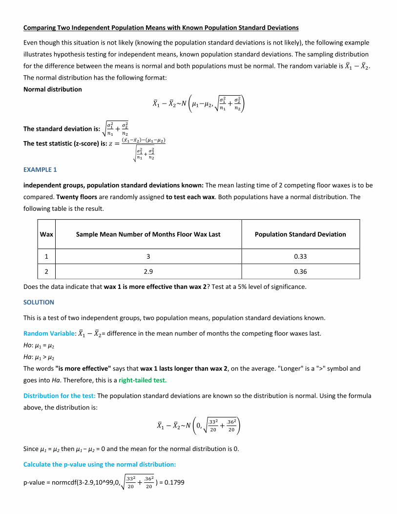
Comparing Two Independent Population Means with Known Population Standard Deviations

Even though this situation is not likely (knowing the population standard deviations is not likely), the following example

illustrates hypothesis testing for independent means, known population standard deviations. The sampling distribution

for the difference between the means is normal and both populations must be normal. The random variable is .

The normal distribution has the following format:

Normal distribution

( √

)

The standard deviation is: √

The test statistic (z-score) is:

√

EXAMPLE 1

independent groups, population standard deviations known: The mean lasting time of 2 competing floor waxes is to be

compared. Twenty floors are randomly assigned to test each wax. Both populations have a normal distribution. The

following table is the result.

Wax Sample Mean Number of Months Floor Wax Last Population Standard Deviation

1 3 0.33

2 2.9 0.36

Does the data indicate that wax 1 is more effective than wax 2? Test at a 5% level of significance.

SOLUTION

This is a test of two independent groups, two population means, population standard deviations known.

Random Variable: = difference in the mean number of months the competing floor waxes last.

Ho: μ1 = μ2

Ha: μ1 > μ2

The words "is more effective" says that wax 1 lasts longer than wax 2, on the average. "Longer" is a ">" symbol and

goes into Ha. Therefore, this is a right-tailed test.

Distribution for the test: The population standard deviations are known so the distribution is normal. Using the formula

above, the distribution is:

( √

)

Since μ1 = μ2 then μ1 − μ2 = 0 and the mean for the normal distribution is 0.

Calculate the p-value using the normal distribution:

p-value = normcdf(3-2.9,10^99,0,√

) = 0.1799

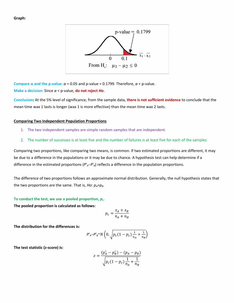
Graph:

Compare α and the p-value: α = 0.05 and p-value = 0.1799. Therefore, α < p-value.

Make a decision: Since α < p-value, do not reject Ho.

Conclusion: At the 5% level of significance, from the sample data, there is not sufficient evidence to conclude that the

mean time wax 1 lasts is longer (wax 1 is more effective) than the mean time wax 2 lasts.

Comparing Two Independent Population Proportions

1. The two independent samples are simple random samples that are independent.

2. The number of successes is at least five and the number of failures is at least five for each of the samples.

Comparing two proportions, like comparing two means, is common. If two estimated proportions are different, it may

be due to a difference in the populations or it may be due to chance. A hypothesis test can help determine if a

difference in the estimated proportions (P′A−P′B) reflects a difference in the population proportions.

The difference of two proportions follows an approximate normal distribution. Generally, the null hypothesis states that

the two proportions are the same. That is, Ho: pA=pB.

To conduct the test, we use a pooled proportion, pc.

The pooled proportion is calculated as follows:

The distribution for the differences is:

P′A−P′B~ ( √

)

The test statistic (z-score) is:

√

EXAMPLE 1: Two population proportions

Two types of medication for hives are being tested to determine if there is a difference in the proportions of adult

patient reactions. Twenty out of a random sample of 200 adults given medication A still had hives 30 minutes after

taking the medication. Twelve out of another random sample of 200 adults given medication B still had hives 30

minutes after taking the medication. Test at a 1% level of significance.

This is a test of 2 population proportions.

Let A and B be the subscripts for medication A and medication B. Then pA and pB are the desired population proportions.

Random Variable:

P'A − P'B = difference in the proportions of adult patients who did not react after 30 minutes to medication A and

medication B.

Ho: pA − pB = 0

Ha: pA − pB ≠ 0

The words "is a difference" tell you the test is two-tailed.

Distribution for the test: Since this is a test of two binomial population proportions, the distribution is normal:

; 1 – pc = 0.92

Therefore, P′A − P′B~ ( √ (

))

P'A−P'B follows an approximate normal distribution.

Calculate the p-value using the normal distribution:

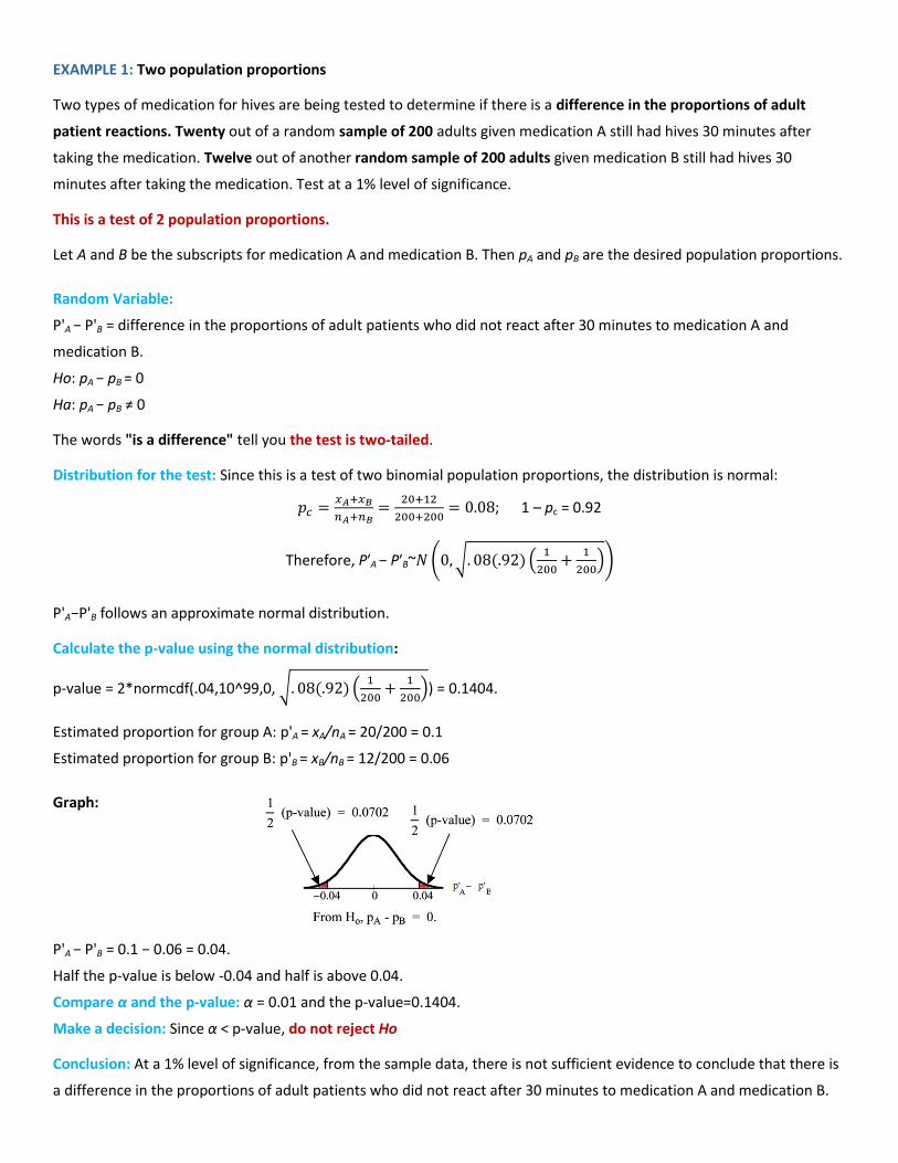
p-value = 2*normcdf(.04,10^99,0, √ (

)) = 0.1404.

Estimated proportion for group A: p'A = xA/nA = 20/200 = 0.1

Estimated proportion for group B: p'B = xB/nB = 12/200 = 0.06

Graph:

P'A − P'B = 0.1 − 0.06 = 0.04.

Half the p-value is below -0.04 and half is above 0.04.

Compare α and the p-value: α = 0.01 and the p-value=0.1404.

Make a decision: Since α < p-value, do not reject Ho

Conclusion: At a 1% level of significance, from the sample data, there is not sufficient evidence to conclude that there is

a difference in the proportions of adult patients who did not react after 30 minutes to medication A and medication B.

Matched or Paired Samples

Summary: This module provides an overview of Hypothesis Testing: Matched or Paired Samples

1. Simple random sampling is used.

2. Sample sizes are often small.

3. Two measurements (samples) are drawn from the same pair of individuals or objects.

4. Differences are calculated from the matched or paired samples.

5. The differences form the sample that is used for the hypothesis test.

6. The matched pairs have differences that either come from a population that is normal or the number of

differences is sufficiently large so the distribution of the sample mean of differences is approximately normal.

In a hypothesis test for matched or paired samples, subjects are matched in pairs and differences are calculated.

The differences are the data.

The population mean for the differences, μd, is then tested using a Student-t test for a single population mean

with n−1 degrees of freedom where n is the number of differences.

The test statistic (t-score) is:

√

EXAMPLE 1: Matched or paired samples

A study was conducted to investigate the effectiveness of hypnotism in reducing pain. Results for randomly selected

subjects are shown in the table. The "before" value is matched to an "after" value and the differences are calculated.

The differences have a normal distribution.

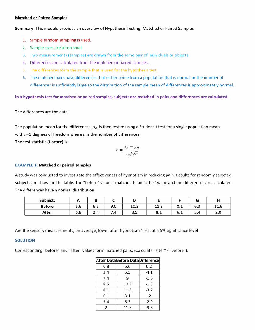
Subject: A B C D E F G H

Before 6.6 6.5 9.0 10.3 11.3 8.1 6.3 11.6

After 6.8 2.4 7.4 8.5 8.1 6.1 3.4 2.0

Are the sensory measurements, on average, lower after hypnotism? Test at a 5% significance level

SOLUTION

Corresponding "before" and "after" values form matched pairs. (Calculate "sfter" - "before").

After Data Before Data Difference

6.8 6.6 0.2

2.4 6.5 -4.1

7.4 9 -1.6

8.5 10.3 -1.8

8.1 11.3 -3.2

6.1 8.1 -2

3.4 6.3 -2.9

2 11.6 -9.6

The data for the test are the differences: {0.2, -4.1, -1.6, -1.8, -3.2, -2, -2.9, -9.6}

The sample mean and sample standard deviation of the differences are: = -3.13 and sd = 2.91

Let μd be the population mean for the differences. We use the subscript d to denote "differences."

Random Variable: = the mean difference of the sensory measurements

Ho: μd = 0 There is no improvement.

Ha: μd > 0 There is improvement.

The score should be lower after hypnotism so the difference ought to be negative to indicate improvement.

Distribution for the test:

The distribution is a student-t with df = n−1 = 8−1 = 7. Use t7. (Notice that the test is for a single population mean.)

Calculate the p-value using the Student-t distribution:

√

√

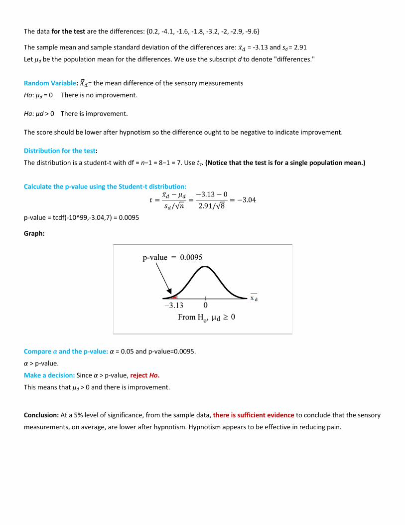
p-value = tcdf(-10^99,-3.04,7) = 0.0095

Graph:

Compare α and the p-value: α = 0.05 and p-value=0.0095.

α > p-value.

Make a decision: Since α > p-value, reject Ho.

This means that μd > 0 and there is improvement.

Conclusion: At a 5% level of significance, from the sample data, there is sufficient evidence to conclude that the sensory

measurements, on average, are lower after hypnotism. Hypnotism appears to be effective in reducing pain.

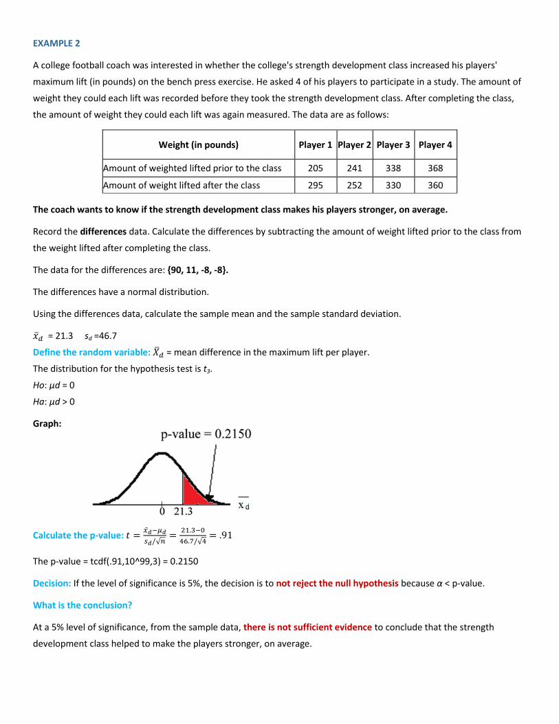
EXAMPLE 2

A college football coach was interested in whether the college's strength development class increased his players'

maximum lift (in pounds) on the bench press exercise. He asked 4 of his players to participate in a study. The amount of

weight they could each lift was recorded before they took the strength development class. After completing the class,

the amount of weight they could each lift was again measured. The data are as follows:

Weight (in pounds) Player 1 Player 2 Player 3 Player 4

Amount of weighted lifted prior to the class 205 241 338 368

Amount of weight lifted after the class 295 252 330 360

The coach wants to know if the strength development class makes his players stronger, on average.

Record the differences data. Calculate the differences by subtracting the amount of weight lifted prior to the class from

the weight lifted after completing the class.

The data for the differences are: {90, 11, -8, -8}.

The differences have a normal distribution.

Using the differences data, calculate the sample mean and the sample standard deviation.

= 21.3 sd =46.7

Define the random variable: = mean difference in the maximum lift per player.

The distribution for the hypothesis test is t3.

Ho: μd = 0

Ha: μd > 0

Graph:

Calculate the p-value:

√

√

The p-value = tcdf(.91,10^99,3) = 0.2150

Decision: If the level of significance is 5%, the decision is to not reject the null hypothesis because α < p-value.

What is the conclusion?

At a 5% level of significance, from the sample data, there is not sufficient evidence to conclude that the strength

development class helped to make the players stronger, on average.

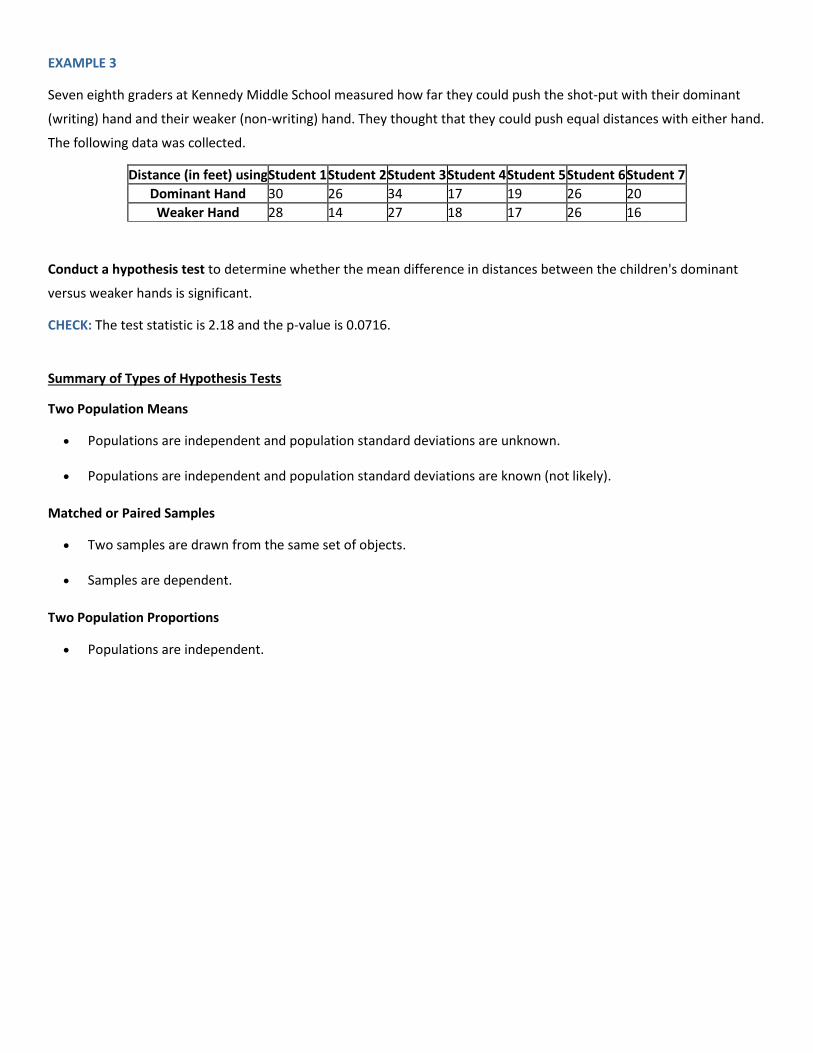
EXAMPLE 3

Seven eighth graders at Kennedy Middle School measured how far they could push the shot-put with their dominant

(writing) hand and their weaker (non-writing) hand. They thought that they could push equal distances with either hand.

The following data was collected.

Distance (in feet) using Student 1 Student 2 Student 3 Student 4 Student 5 Student 6 Student 7

Dominant Hand 30 26 34 17 19 26 20

Weaker Hand 28 14 27 18 17 26 16

Conduct a hypothesis test to determine whether the mean difference in distances between the children's dominant

versus weaker hands is significant.

CHECK: The test statistic is 2.18 and the p-value is 0.0716.

Summary of Types of Hypothesis Tests

Two Population Means

Populations are independent and population standard deviations are unknown.

Populations are independent and population standard deviations are known (not likely).

Matched or Paired Samples

Two samples are drawn from the same set of objects.

Samples are dependent.

Two Population Proportions

Populations are independent.