Hypothesis Testing Quantitative Methods in HPELS 440:210.

Hypothesis Testing

Quantitative Methods in HPELS

440:210

Agenda

Introduction Hypothesis Testing General Process Errors in Hypothesis Testing One vs. Two Tailed Tests Effect Size and Power Instat Example

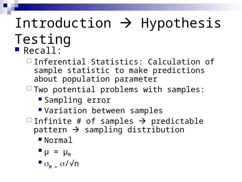
Introduction Hypothesis Testing Recall:

Inferential Statistics: Calculation of sample statistic to make predictions about population parameter

Two potential problems with samples: Sampling error Variation between samples

Infinite # of samples predictable pattern sampling distribution

Normal µ = µM M = /√n

Introduction Hypothesis Testing Common statistical procedure Allows for comparison of means General process:

1. State hypotheses

2. Set criteria for decision making

3. Collect data calculate statistic

4. Make decision

Introduction Hypothesis Testing

Remainder of presentation will use following concepts to perform a hypothesis test:

Z-score Probability Sampling distribution

Agenda


General Process of HT Step 1: State hypotheses Step 2: Set criteria for decision making Step 3: Collect data and calculate

statistic Step 4: Make decision

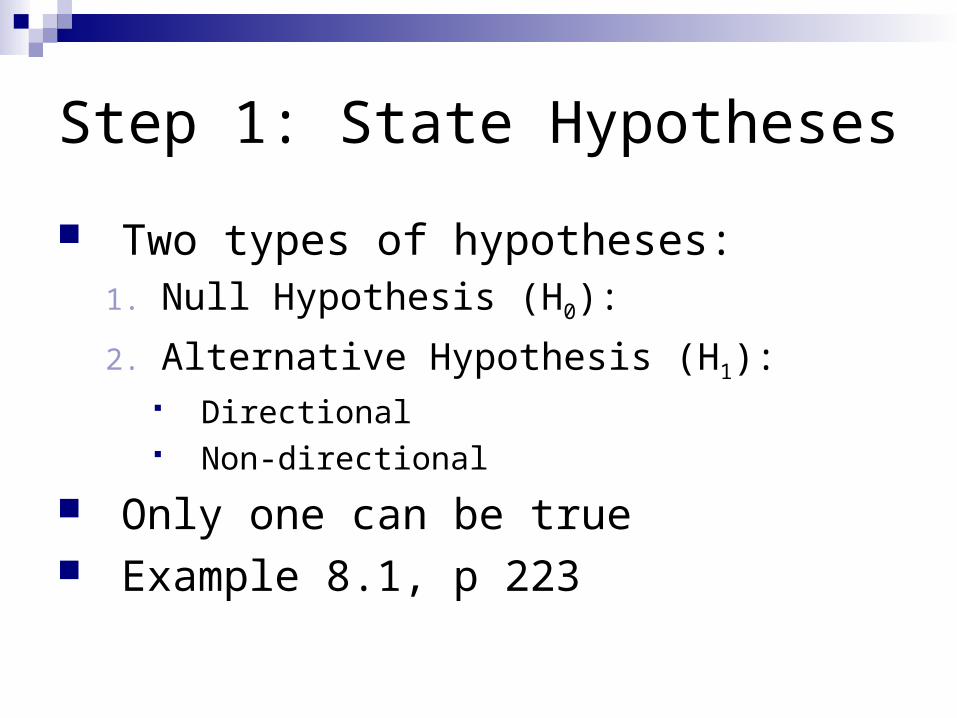
Step 1: State Hypotheses

Two types of hypotheses:1. Null Hypothesis (H0):

2. Alternative Hypothesis (H1): Directional Non-directional

Only one can be true Example 8.1, p 223

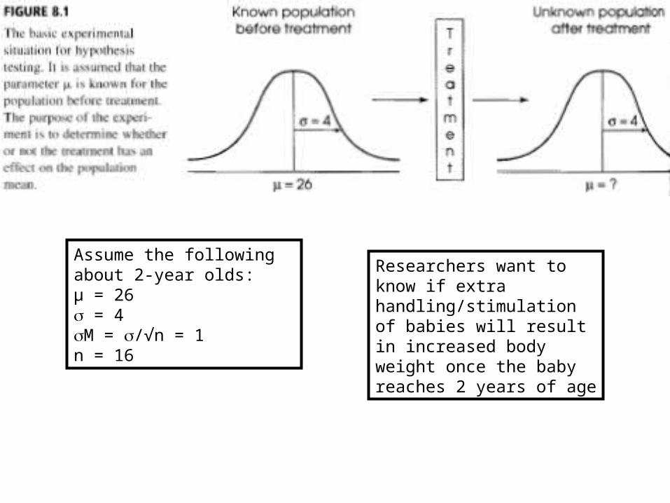
Assume the following about 2-year olds:µ = 26 = 4M = /√n = 1n = 16

Researchers want to know if extra handling/stimulation of babies will result in increased body weight once the baby reaches 2 years of age

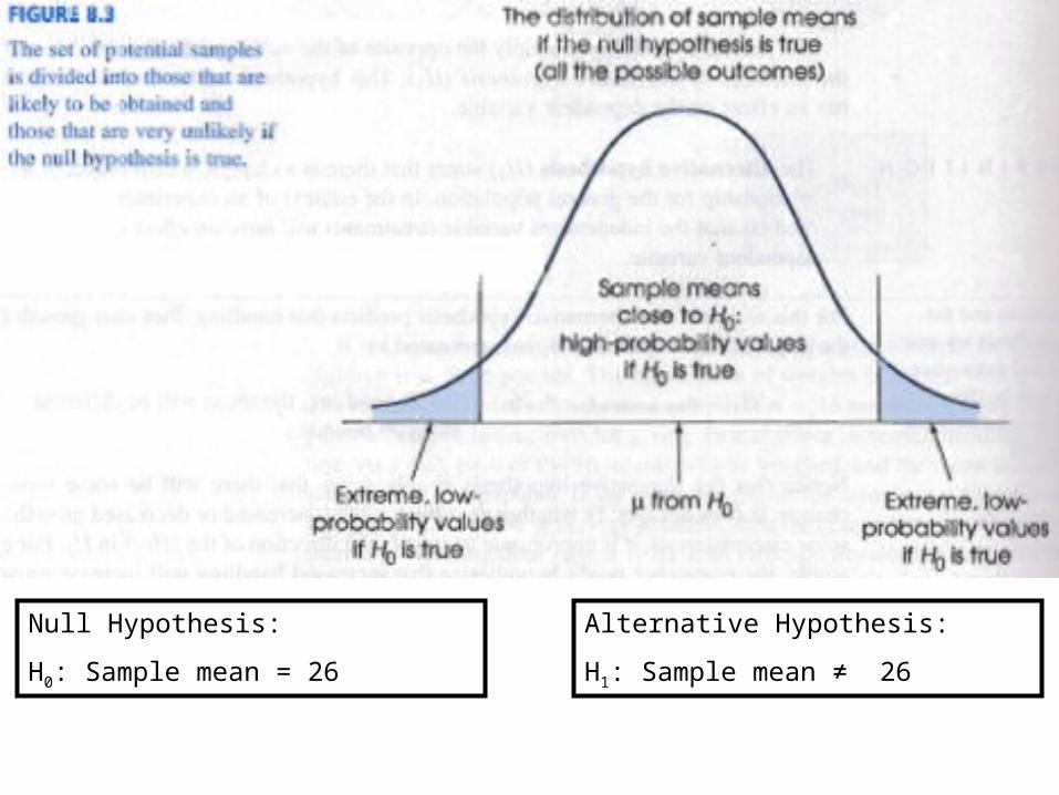
Null Hypothesis:

H0: Sample mean = 26

Alternative Hypothesis:

H1: Sample mean ≠ 26

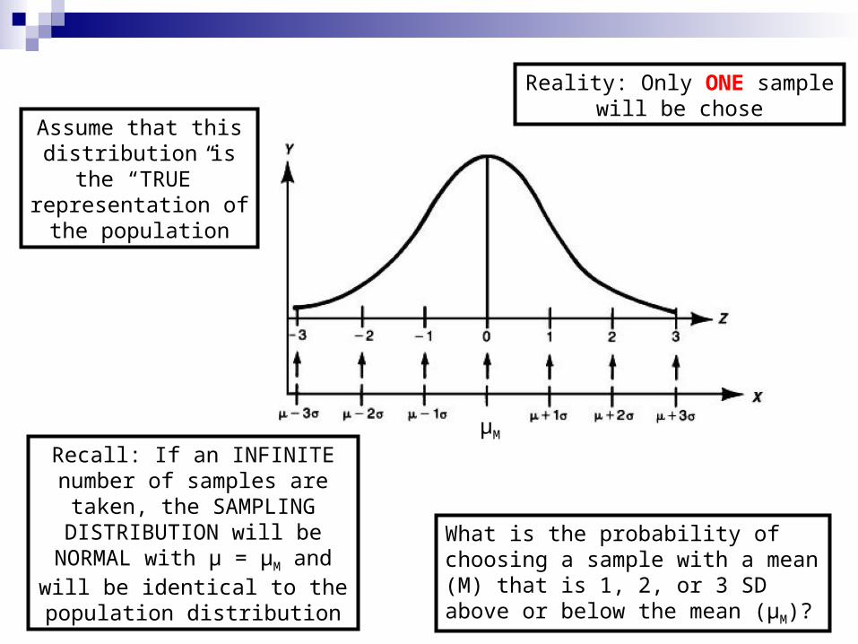
Assume that this distribution is the

“TRUE” representation of the population

Recall: If an INFINITE number of samples are taken, the

SAMPLING DISTRIBUTION will be NORMAL with µ = µM and will

be identical to the population distribution

Reality: Only ONE sample will be chose

What is the probability of choosing a sample with a mean (M) that is 1, 2, or 3 SD above or below the mean (µM)?

µM

µM µM

µM

p(M > µM + 1 ) = 15.87% p(M > µM + 2 ) = 2.28%

p(M > µM + 3 ) = 0.13%

It is much more PROBABLE that our sample mean (M) will fall closer to the mean of the means (µM) as well as the population mean (µ)

µM

Inferential statistics is based on the assumption that our sample is PROBABLY representative of

the population

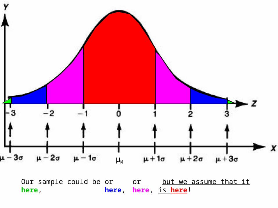
Our sample could be here, or here, or here, but we assume that it is here!

µM


If true (no effect):

1.) It is PROBABLE that the sample mean (M) will fall in the middle

2.) It is IMPROBABLE that the sample mean (M) will fall in the extreme edges

H1: Sample mean ≠ 26

If true (effect):

1.) It is PROBABLE that the sample mean (M) will fall in the extreme edges

2.) It is IMPROBABLE that the sample mean (M) will fall in the middle

Assume that M = 30 lbs

(n = 16)

µ = 26 M = 30

Accept or reject?


What criteria do you use to make the decision?

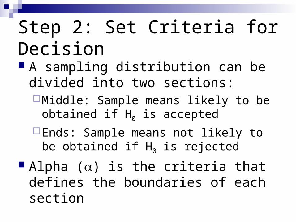
Step 2: Set Criteria for Decision A sampling distribution can be divided into

two sections:Middle: Sample means likely to be obtained if

H0 is accepted

Ends: Sample means not likely to be obtained if H0 is rejected

Alpha () is the criteria that defines the boundaries of each section

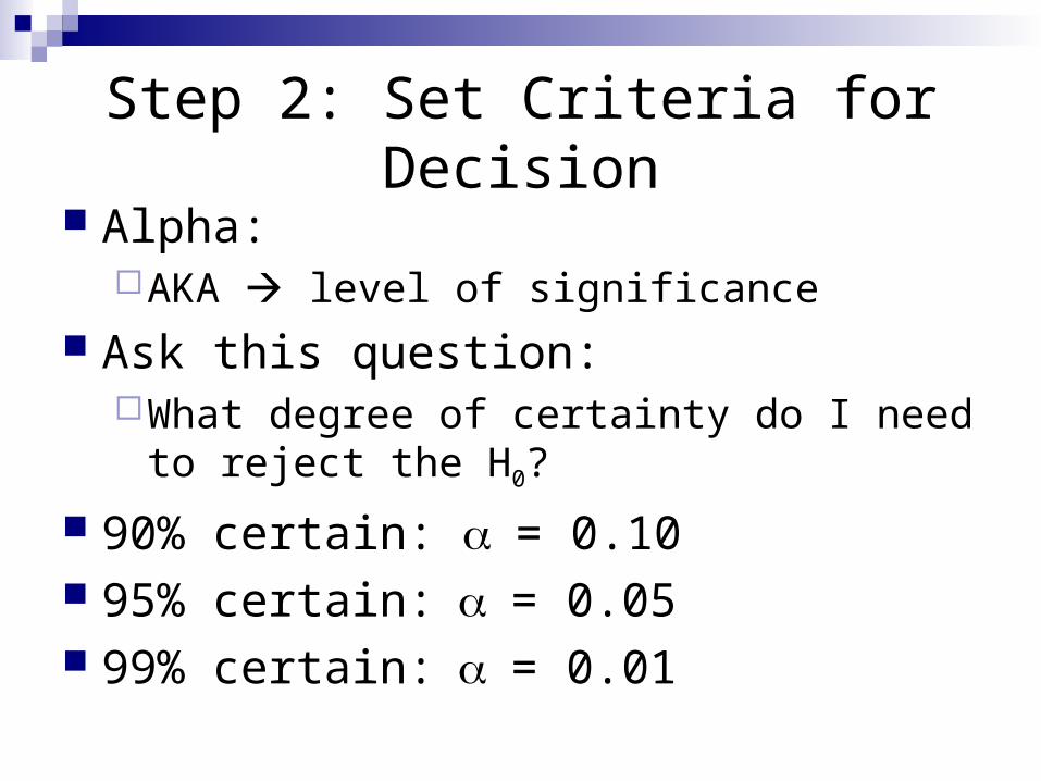
Step 2: Set Criteria for Decision Alpha:

AKA level of significance Ask this question:

What degree of certainty do I need to reject the H0?

90% certain: = 0.10 95% certain:= 0.05 99% certain:= 0.01

Step 2: Set Criteria for Decision

As level of certainty increases: decreasesMiddle section gets largerCritical regions (edges) get smaller

Bottom line: A larger test statistic is needed to reject the H0

Step 2: Set Criteria for Decision Directional vs. non-

directional alternative hypotheses

Directional: H1: M > or < X

Non-directional:H1: M ≠ X

Which is more difficult to reject H0?


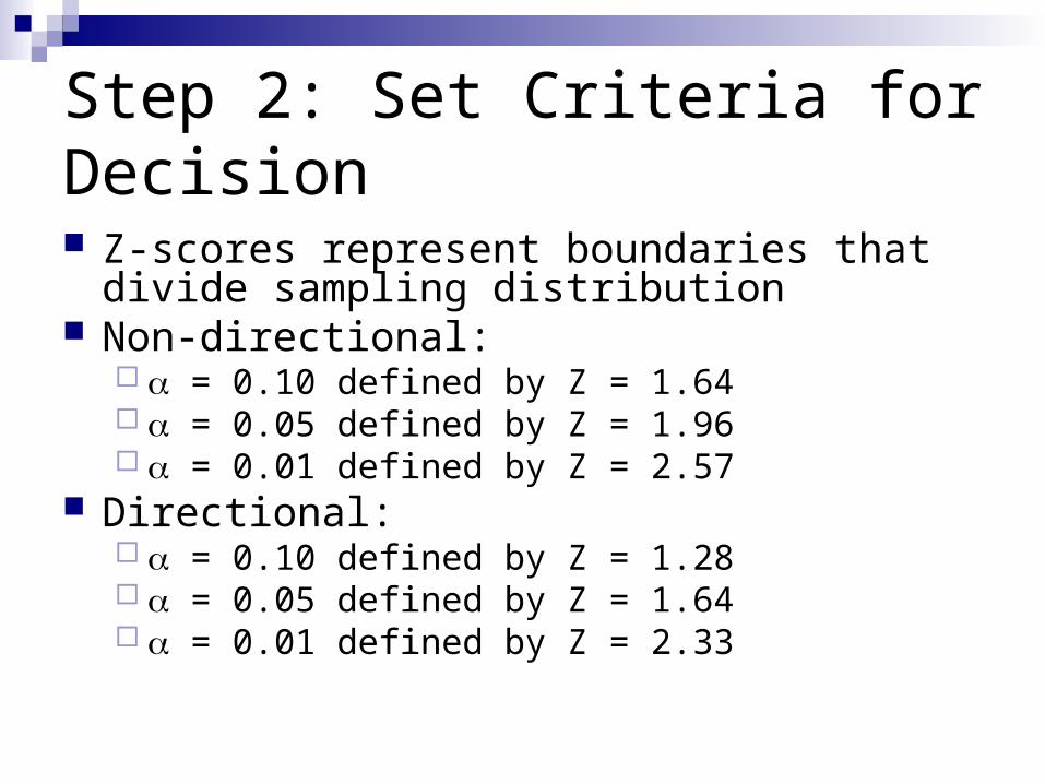
Z-scores represent boundaries that divide sampling distribution

Non-directional: = 0.10 defined by Z = 1.64 = 0.05 defined by Z = 1.96 = 0.01 defined by Z = 2.57

Directional: = 0.10 defined by Z = 1.28 = 0.05 defined by Z = 1.64 = 0.01 defined by Z = 2.33

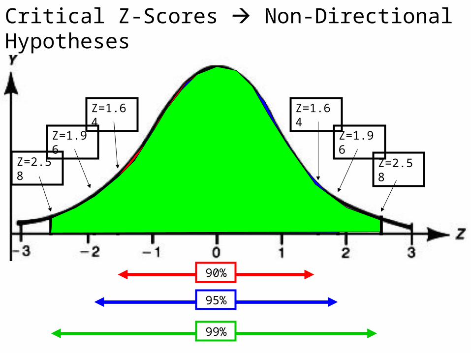
Critical Z-Scores Non-Directional Hypotheses

90%

95%

99%

Z=1.64

Z=1.96

Z=2.58

Z=1.64

Z=1.96

Z=2.58

Critical Z-Scores Directional Hypotheses

Z=1.28

Z=1.64

Z=2.34

90%

95%

99%


Where should you set alpha?Exploratory research 0.10Most common 0.050.01 or lower?

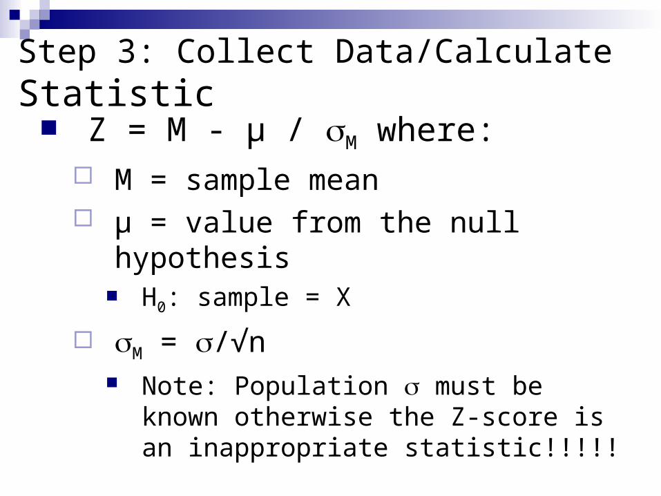
Step 3: Collect Data/Calculate Statistic Z = M - µ / M where:

M = sample mean µ = value from the null hypothesis

H0: sample = X

M = /√n Note: Population must be known

otherwise the Z-score is an inappropriate statistic!!!!!

Example 8.1 Continued

Step 3: Collect Data/Calculate Statistic

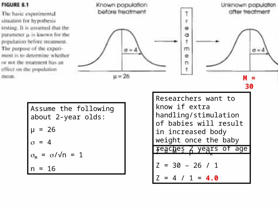
Assume the following about 2-year olds:

µ = 26

= 4

M = /√n = 1

n = 16

Researchers want to know if extra handling/stimulation of babies will result in increased body weight once the baby reaches 2 years of age

M = 30

Z = M - µ / M

Z = 30 – 26 / 1

Z = 4 / 1 = 4.0

Process:

1. Draw a sketch with critical Z-score Assume non-directional Alpha = 0.05

2. Plot Z-score statistic on sketch

3. Make decision

Step 4: Make Decision

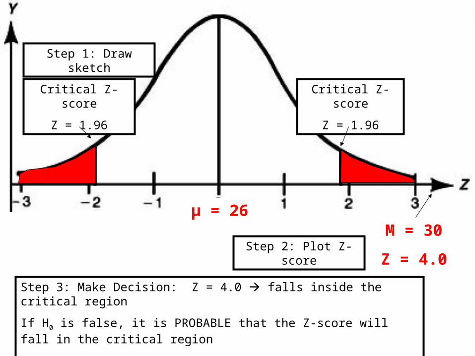
µ = 26M = 30

Z = 4.0

Step 1: Draw sketch

Critical Z-score

Z = 1.96

Critical Z-score

Z = 1.96

Step 3: Make Decision: Z = 4.0 falls inside the critical region

If H0 is false, it is PROBABLE that the Z-score will fall in the critical region

ACCEPT OR REJECT?

Step 2: Plot Z-score

Agenda


Errors in Hypothesis Testing

Recall Problems with samples:Sampling errorVariability of samples

Inferential statistics use sample statistics to predict population parameters

There is ALWAYS chance for error

Errors in Hypothesis Testing

There is potential for two kinds of error:

1. Type I error

2. Type II error

Type I Error Rejection of a true H0

Recall alpha = certainty of rejecting H0 Example:

Alpha = 0.05 95% certain of correctly rejecting the H0

Therefore 5% certain of incorrectly rejecting the H0

Alpha maybe thought of as the “probability of making a Type I error

Consequences:False reportWaste of time/resources

Type II Error

Acceptance of a false H0

Consequences:Not as serious as Type I errorResearcher may repeat experiment if type II

error is suspected

Agenda


One vs. Two-Tailed Tests

One-Tailed (Directional) Tests:Specify an increase or decrease in the

alternative hypothesisAdvantage: More powerfulDisadvantage: Prior knowledge required

One vs. Two-Tailed Tests

Two-Tailed (Non-Directional) Tests:Do not specify an increase or decrease in the

alternative hypothesisAdvantage: No prior knowledge requiredDisadvantage: Less powerful

Agenda


Statistical Software p-value The p-value is the probability of a type I

error Recall alpha ()

Recall Step 4: Make a Decision

Recall Step 4: Make a Decision

If the p-value > accept the H0

Probability of type I error is too highResearcher is not “comfortable” stating that

differences are real and not due to chance

If the p-value < reject the H0

Probability of type I error is low enoughResearcher is “comfortable” stating that

differences are real and not due to chance

Statistical vs. Practical Significance

Distinction:

1. Statistical significance: There is an acceptably low chance of a type I error

2. Practical significance: The actual difference between the means are not trivial in their practical applications

Practically Significant? Knowledge and experience Examine effect size

The magnitude of the effect Examples of measures of effect size:

Eta-squared (2) Cohen’s d R2

Interpretation of effect size: 0.0 – 0.2 = small effect 0.21 – 0.8 = moderate effect > 0.8 = large effect

Examine power of test

Statistical Power

Statistical power: The probability that you will correctly reject a false H0

Power = 1 – where = probability of type II error

Example: Statistical power = 0.80 therefore:80% chance of correctly rejecting a false H0

20% of accepting a false H0 (type II error)

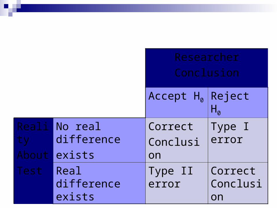
Researcher

Conclusion

Accept H0 Reject H0

Reality

About

Test

No real difference

exists

Correct

Conclusion

Type I error

Real difference exists

Type II error

Correct Conclusion

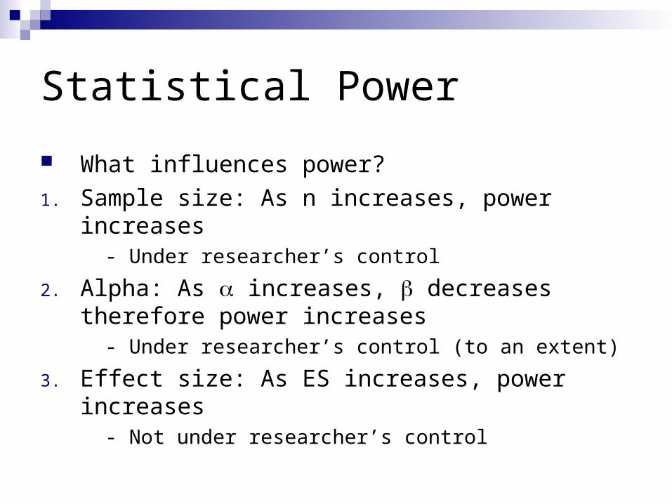
Statistical Power

What influences power?

1. Sample size: As n increases, power increases- Under researcher’s control

2. Alpha: As increases, decreases therefore power increases

- Under researcher’s control (to an extent)

3. Effect size: As ES increases, power increases- Not under researcher’s control

Statistical Power

How much power is desirable? General rule: Set as 4* Example:

= 0.05, therfore = 4*0.05 = 0.20Power = 1 – = 1 – 0.20 = 0.80

Statistical Power

What if you don’t have enough power? More subjects

What if you can’t recruit more subjects and you want to prevent not having enough power? Estimate optimal sample size a priori See statistician with following information:

Alpha Desired power Knowledge about effect size what constitutes a small,

moderate or large effect size relative to your dependent variable

Statistical Power

Examples:

1. Novice athlete improves vertical jump height by 2 inches after 8 weeks of training

2. Elite athlete improves vertical jump height by 2 inches after 8 weeks of training

Agenda

Introduction Hypothesis Testing General Process Errors in Hypothesis Testing One vs. Two Tailed Tests Instat Example

Instat Type data from sample into a column.

Label column appropriately. Choose “Manage” Choose “Column Properties” Choose “Name”

Choose “Statistics” Choose “Simple Models”

Choose “Normal, One Sample”

Layout Menu: Choose “Single Data Column”

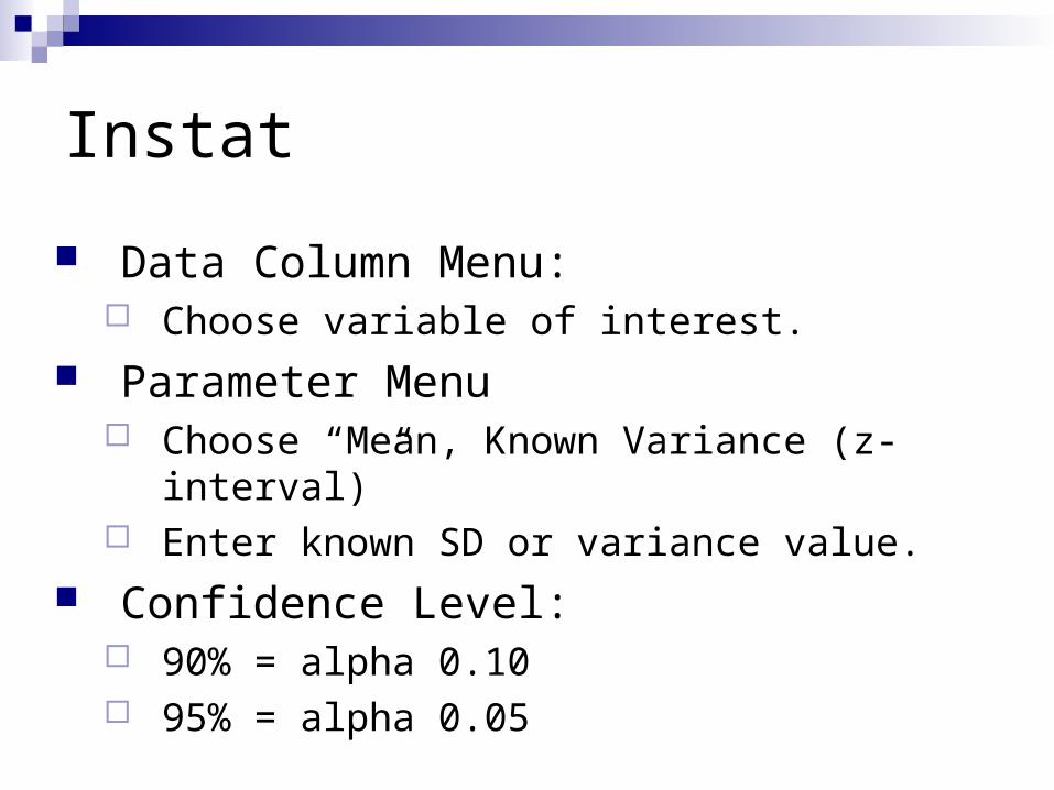
Instat

Data Column Menu: Choose variable of interest.

Parameter Menu Choose “Mean, Known Variance (z-interval)” Enter known SD or variance value.

Confidence Level: 90% = alpha 0.10 95% = alpha 0.05

Instat

Check “Significance Test” box: Check “Two-Sided” if using non-directional

hypothesis. Enter value from null hypothesis.

What population value are you basing your sample comparison?

Click OK. Interpret the p-value!!!

Agenda

Introduction Hypothesis Testing General Process Errors in Hypothesis Testing One vs. Two Tailed Tests Instat Example

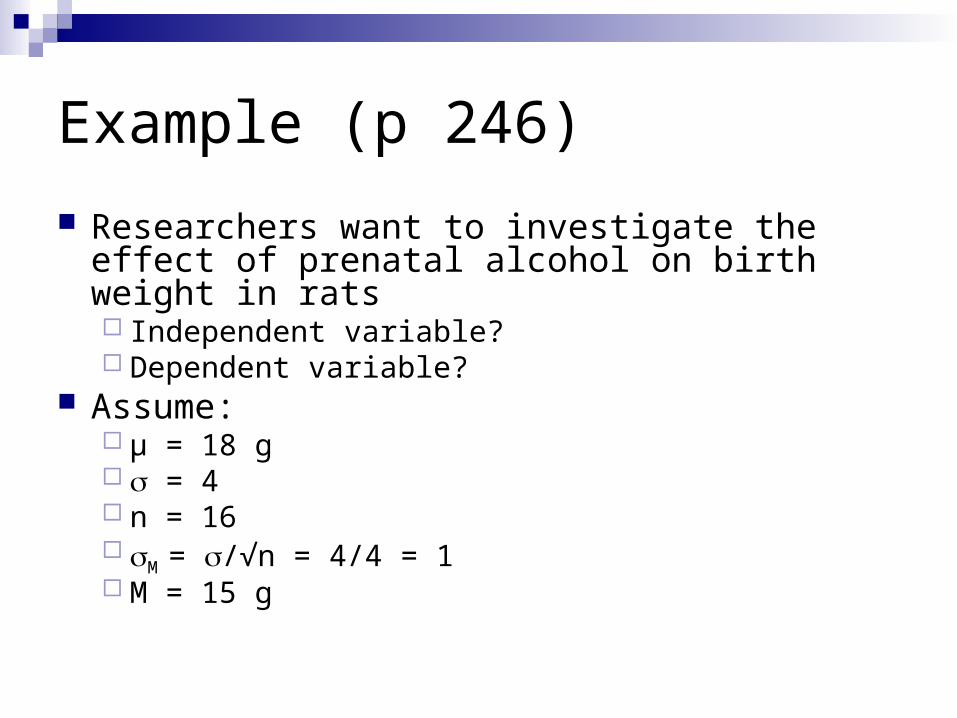
Example (p 246)

Researchers want to investigate the effect of prenatal alcohol on birth weight in rats Independent variable? Dependent variable?

Assume: µ = 18 g = 4 n = 16 M = /√n = 4/4 = 1 M = 15 g

Step 1: State hypotheses (directional or non-directional)

H0: µalcohol = 18 g

H1: µalcohol ≠ 18 g

Step 2: Set criteria for decision making

Alpha () = 0.05

Step 3: Sample data and calculate statistic

Z = M - µ / M

Z = 15 – 18 / 1 = -3.0

Step 4: Make decision

Does Z-score fall inside or outside of the critical region?

Accept or reject?

Statistical Software:

p-value = 0.02 Accept or reject?

p-value = 0.15 Accept or reject?

Homework

Problems: 3, 5, 6, 7, 8, 11, 21

Hypothesis Testing Quantitative Methods in HPELS 440:210.

Documents

Transcript of Hypothesis Testing Quantitative Methods in HPELS 440:210.