HYPHOREIC ZONE HYDRAULIC TESTING:

RIVER TAME, BIRMINGHAM, UK

by

Jennifer Laura Whelan

Submitted in part fulfilment

of the requirements for an

MSc in Hydrogeology

September 2007

School of Earth Sciences

University of Birmingham

ii

Abstract

The hyporheic zone is a dynamic ecotone, within which important physical, chemical and

biological processes occur. It is believed that the hyporheic zone has the potential to naturally

attenuate contaminants and limit their exchange between groundwater and surface waters.

Fieldwork was conducted on an urbanised stretch of the River Tame in north Birmingham in

order to characterise the hydraulic properties of the unconfined sandstone aquifer and river bed

sediments. The hydraulic conductivity of the Kidderminster Sandstone was calculated as 2 m/d.

Groundwater head measurements indicated that the Tame was gaining along the entire study

reach with a mean hydraulic gradient of 0.1036. The river bed sediments were found to be very

heterogeneous with their hydraulic conductivities ranging from 0.61 m/d to 52.96 m/d, the mean

hydraulic conductivity is 5.28 m/d. Groundwater flow modeling of a proposed pump test next to

the river indicated that pumping at a rate of 200 m3/d will reduce the observed hydraulic

gradients by between 2.07% and 48.51%, this is very much dependent on the hydraulic

parameters for the river bed sediments, and to a lesser extent, the superficial drift deposits.

iii

Acknowledgements

I would like to thank my supervisors Professor Rae Mackay, Dr Richard Greswell and Dr

Veronique Durand for all their support and guidance throughout the project.

Thanks to Adam Bates, Daniel Welch and Charles Bacon for help in the field.

iv

Table of Contents

Abstract………………………………………………………………………………………………………ii

Acknowledgements…………………………………………………………………………………………iii

Chapter 1. Introduction…………………………………………………………………………....1

1.1 Project Background…………………………………………………………………... 1

1.2 Project Aims and Objectives..........................................................................................1

1.3 Approach………………………………………………………………………………2

Chapter 2. Groundwater – Surface Water Interactions……………………………………………4

2.1 Introduction……………………………………………………………………………4

2.2 Understanding Groundwater-Surface Water Interactions……………………………..4

2.2.1 Conceptual Models………………………………………………………….5

2.3 The Hyporheic Zone…………………………………………………………………..7

2.3.1 Definition……………………………………………………………………7

2.3.2 Mixing in the Hyporheic Zone………………………………………………9

2.3.3 Groundwater-Surface Water Contamination………………………………12

2.4 Methods to Characterise Groundwater-Surface Water Exchange…………………...13

2.5 Estimating Groundwater-Surface Water Exchange………………………………….15

2.6 Conclusions…………………………………………………………………………..16

Chapter 3. Site Setting…………………………………………………………………………...18

3.1 Study Setting…………………………………………………………………………18

3.2 Study Site…………………………………………………………………………….19

3.3 Regional Geology……………………………………………………………………20

3.3.1 Sherwood Sandstone Group……………………………………………….22

3.3.2 Drift………………………………………………………………………..24

3.4 Regional Hydrogeology……………………………………………………………...25

3.5 Local Geology………………………………………………………………………..28

3.6 Local Hydrogeology…………………………………………………………………30

3.7 Hydrology……………………………………………………………………………31

v

Chapter 4. Data Collection……………………………………………………………………….33

4.1 Introduction…………………………………………………………………………..33

4.2 Borehole Installation…………………………………………………………………33

4.3 Pump Test……………………………………………………………………………35

4.4 Analysis of Pump Test Data…………………………………………………………36

4.5 Construction of Riverbed Mini Drive Point Piezometers (MDP’s)………………….38

4.6 Installation of MDP’s………………………………………………………………...42

4.7 Hydraulic Gradient…………………………………………………………………...44

4.8 Falling Head Tests…………………………………………………………………...45

4.9 Analysis of Falling Head Test Data………………………………………………….46

Chapter 5. Fieldwork Results…………………………………………………………………….49

5.1 Introduction…………………………………………………………………………..49

5.2 Pump Test……………………………………………………………………………49

5.3 Piezometer Installation……………………………………………………………….51

5.4 Groundwater Head Measurements…………………………………………………...52

5.5 Hydraulic Gradients………………………………………………………………….54

5.6 Falling Head Tests…………………………………………………………………...55

5.7 Conclusions…………………………………………………………………………..59

Chapter 6. Modelling…………………………………………………………………………….61

6.1 Introduction…………………………………………………………………………..61

6.2 Basic Conceptual Model……………………………………………………………..61

6.2.1 Aquifer Geometry………………………………………………………….62

6.2.2 Boundary Conditions/Initial Heads………………………………………...63

6.2.3 Aquifer Hydraulic Properties………………………………………………64

6.2.4 Model Grid…………………………………………………………………65

6.3 Transient Model……………………………………………………………………...67

6.4 Results………………………………………………………………………………..68

6.5 Use of Model as a Predictive Tool…………………………………………………...72

6.6 Sensitivity Analysis………………………………………………………………….73

vi

6.7 Conclusions…………………………………………………………………………..74

Chapter 7. Conclusions…………………………………………………………………………..75

7.1 Summary……………………………………………………………………………..76

7.2 Future Work………………………………………………………………………….77

References

Appendices

vii

List of Figures

2.2.1 Four basic conceptual models indicating direction of flow between a stream channel and the

underlying aquifer; A, Gaining or effluent stream; B, Losing or influent stream; C, Groundwater

through flow; D, Disconnected stream.

6

2.3.1 Schematic diagram of the hyporheic zone indicating the mixing of surface waters and groundwater

within the region (from Smith, 2005)

8

2.3.2 Hyporheic zone at two spatial scales (arrows indicate the water flow paths); A, the reach scale,

upwelling and downwelling zones alternate; B, the sediment scale, microbial and chemical processes

occur, creating microscale gradients (Adapted from Boulton et al, 1998)

10

3.1.1 Map of the River Tame catchment indicating the extent of urban land use (from SMURF 2005) 18

3.2.1 Location of study site 19

3.2.2 Location of borehole within the study reach 20

3.3.1 Sketch map of the solid geology of the Birmingham area (from Powell et al, 2000) 21

3.3.2 Regional drift map of Birmingham and surrounding area 25

3.4.1 Map of Birmingham region indicating the location of the main aquifer and the study site (adapted

from Ellis et al, 2007)

26

3.4.2 Conceptual model of groundwater flow in the Birmingham aquifer (from Greswell, 1992) 27

3.5.1 A: Map of the bedrock at the study site; B: map op drift cover at the study site 29

3.6.1 Distribution of groundwater head in the study area (from Ellis 2002) 30

3.7.1 Study site looking upstream from the Gavin Way Bridge, the river has been straightened as part of

flood defence work carried out in the area

31

4.2.1 Installation of borehole on the north bank of the River Tame; A, Drill bits and casing used; B,

Drilling the borehole; C, Borehole log indicating depth below ground level of different sediment

layers and the depths of plain and slotted casing

34

4.5.1 Schematic diagram of MDP design. The 1m MDP (on the left) is inserted to a depth of 1m below the

stream bed, the open section is at a depth of 1m, the position of the multi-level samplers are placed at

10cm intervals over a depth of 1m. The 0.5m MDP (on the right) is inserted to a depth of 1m below

the stream bed, the open section is at a depth of 0.5m, multi-level samplers are placed at 10cm

intervals over a depth of 1m

39

4.5.2 Open section of MDP. 100 micron nylon mesh is held in place by stainless steel wire to cover the

drilled holes

40

4.5.3 Design and attachment of sampling tube to the MDP 41

4.5.4 Completed multi-level, mini drive point piezometer 42

4.6.1 Installation of piezometer, a fence driver post is used to drive the steel pole to the required depth 43

4.8.1 Falling head test on piezometer. 10cm intervals were marked on the wooden board held next to the

piezometer to allow the change in head level to be easily measured

46

4.9.1 Hvorslev piezometer test; (a) piezometer geometry; (b) graphical method for analysis of T0 (from

Hiscock, 2005)

48

5.2.1 Discharge period of pump test 49

5.2.2 Recovery period of pump test 50

5.3.1 Map of study site indicating the location of all the piezometers installed on site for this project 51

5.4.1 Plot of groundwater head versus depth, indicates the heterogeneous nature of the river bed sediments.

Individual piezometer profiles are picked out.

53

5.6.1 Cumulative probability plot of river bed hydraulic conductivity values indicating a log normal

distribution, however this does not include the value calculated at P+005-1

58

6.2.1 Basic geometry used in modelling (not to scale) 63

viii

6.2.2 Position of constant head boundaries on model grid 64

6.2.3 Location of model grid in relation to the study area (top); detailed grid mesh around borehole, river

and piezometers (below)

66

6.4.1 Drawdown contours (layer 3 of model, stress period 8, time step 10). 68

6.4.2 Drawdown curves for selected piezometers from initial model run, as expected piezometers nearest to

the borehole show the highest drawdown.

69

6.4.3 Drawdown curves for selected piezometers from second model run (the two river bed layers have

been assigned different values) as expected piezometers nearest to the borehole show the highest

drawdown.

71

List of Tables

3.3.1 Stratigraphic sequence of the Triassic and lower Jurassic in the region (adapted from Powell et al,

2000)

22

5.2.1 Calculated transmissivity and estimated hydraulic conductivity values from discharge and recovery

periods of the pump test

50

5.5.1 Calculated hydraulic gradients for each piezometer. Groundwater head measured as height above

datum (river water level)

54

5.6.1 Hydraulic conductivity estimates from falling head test. ? indicates failed, inconclusive or no test. 57

6.2.1 Elevations of stratigraphical units used in model (adapted from Lydon, 2006) 62

6.2.2 Initial Hydraulic conductivity values used for model layers 65

6.3.1 Stress period set up for transient model 67

6.4.2 Summary of hydraulic gradient changes observed in river bed sediments when pumping at 200m3/d

70

6.4.3 Summary of hydraulic gradient changes observed in river bed sediments when pumping at 200m3/d

during second model run

71

Appendices

Appendix 1 – Pump Test Data

Appendix 2 – Pump Test Analysis

Appendix 3 – List of Piezometer Depths and Lengths

Appendix 4 – Falling Head Test Data

Appendix 5 – Analysis of Falling Head Test Data

Appendix 6 – Summary of Piezometer Data Results

Appendix 7 – Model Piezometer Data

Appendix 8 – Site Photographs

1

Chapter 1. Introduction

1.1 Project Background

The hyporheic zone represents a critical interface between groundwater and surface water. It is a

dynamic ecotone within which important microbial and geochemical processes take place, which

are thought to have an effect on contaminant transport due to natural attenuation. The

introduction of the EU Water Framework Directive has led to a more integrated management of

surface and groundwater resources, increasing the need to understand contaminant movement

through the hyporheic zone.

This project forms part of the early stages of the SWITCH project which aims to improve the

conceptual understanding of the hyporheic zone and its potential to naturally attenuate pollutants.

The focus is on a research site currently being developed on an urbanised stretch of the River

Tame in north Birmingham.

Bank-side extraction of groundwater will be carried out at the study site. This will perturb the

groundwater-surface water exchanges in a controlled manner to assess the natural attenuation

capacity of the hyporheic zone. The transport of injected tracers, solutes and contaminants will

be monitored during these tests which are expected to take place over a prolonged period of time.

1.2 Project Aims and Objectives

This project aims to investigate the hydraulic properties of the geological units within the study

area. This will then be used to build a basic numerical model of the aquifer/river system with

which the effects of hydraulic testing on the hyporheic zone can be assessed. In particular the

2

model will look at the changes in hydraulic gradient below the river bed due to groundwater

abstractions, as this will determine the pump rate used in future experiments at the study site.

To meet these aims the following objectives must be met:

A desk study should be conducted to gain an understanding of the regional and site

geological, hydrogeological and hydrological conditions.

A detailed characterisation of the hydraulic properties of the site should be conducted in

the field to collect data for a numerical groundwater flow model.

The model should test the effect pump tests will have on the observed hydraulic gradients

below the river bed.

1.3 Approach

The objectives for this project were met by carrying out a combination of field studies, desk

based study and computer modelling. Previous work on the site by Ellis (2002), Lydon (2006)

and Conran (2006) provided a good understanding of the methodologies used for data collection

in the field.

A literature review (Chapter 2) provided an insight into the current understanding of

groundwater-surface water interactions and the processes occurring within the hyporheic zone

which affect the exchange of water. Chapter 3 examines the study area and gives a

comprehensive review of the geological, hydrogeological and hydrological knowledge of the

regional and local area.

3

The methods used to collect and analyse data are given in detail in Chapter 4, with the results

detailed in Chapter 5. The subsequent modelling of the study area is described in Chapter 6.

4

Chapter 2. Groundwater – Surface Water Interactions

2.1 Introduction

The importance of understanding groundwater-surface water interactions has increased with the

introduction of the Water Framework Directive (WFD) in December 2000. The WFD has the

primary goal of ensuring that water bodies achieve the environmental objectives set out in

Article 4 of the directive, these include good chemical and quantitative status of groundwater

bodies and good chemical and ecological status for surface water bodies (Environment Agency,

2002). Member states are required to ensure that water bodies achieve these objectives by 2015,

therefore there is a great necessity to improve our understanding of how groundwater and surface

water bodies interact, particularly in terms of the potential for attenuation of pollutants (Smith,

2005). Groundwater and surface water are not isolated components of the hydrologic system, and

therefore development or contamination of one will commonly affect the other (Sophocleous,

2002). By combining the disciplines of hydrogeology, hydrology and ecology a more

comprehensive understanding of groundwater-surface water interactions is being achieved,

which will lead to more effective management of water resources.

This chapter will review the current understanding of groundwater-surface water interactions, in

particular looking at the hyporheic zone and its potential for natural attenuation of pollutants.

Methods for quantifying groundwater-surface water flow will also be discussed.

2.2 Understanding Groundwater-Surface Water Interactions

To understand the complex nature of groundwater-surface water interactions a number of

physical factors must be considered, these include climate, topography, geology and the

5

position of the surface water body in relation to the groundwater flow system (Winter, 2000;

Sophocleous, 2002). Woessner (2000) has stated that the controlling factors for groundwater

flow to a river channel are:

the distribution and magnitude of the hydraulic conductivities within the river channel,

the associated fluvial plain sediments and the underlying bedrock

the relation of stream stage to the adjacent groundwater head

the geometry and position of the river channel within the fluvial plain

2.2.1 Conceptual Models

There are four basic conceptual models which describe the flow between groundwater and a

stream channel. These models, shown in Fig 2.2.1, are based on the relationship between the

stream stage and the groundwater head.

A gaining or effluent stream has a groundwater head at the channel interface which is greater

than the stream stage (Fig 2.2.1a). This results in flow from the aquifer into the stream. These

streams are often sensitive to nearby groundwater abstractions, which alter the groundwater

heads and affect the contribution of groundwater discharge to the streams base flow (Griffiths et

al, 2006; Winter et al, 1998).

A losing or influent stream has a groundwater head at the channel interface which is lower than

the stream stage (Fig 2.2.1b). This results in flow from the stream to the aquifer. These streams c

can be at risk from climate change and may dry out during prolonged dry periods (Wheater et al,

2007).

6

Figure 2.2.1 Four basic conceptual models indicating direction of flow between a stream channel and the underlying aquifer;

A, Gaining or effluent stream; B, Losing or influent stream; C, Groundwater through flow; D, Disconnected stream.

7

Groundwater through flow occurs when the groundwater head is higher than the stream stage on

one bank but lower on the other (Fig 2.2.1c). These conditions commonly exist when the stream

channel cuts perpendicular to the fluvial-plain groundwater flow field (Sophocleous, 2002).

Under some conditions there may be no hydraulic connectivity of the groundwater with the

stream (Fig 2.2.1d). These disconnected streams typically occur in very arid conditions, where

low water tables exist. Water may still be exchanged between the two systems by seepage

through the unsaturated zone.

These conceptual models define the direction of water flow between the aquifer and stream. The

magnitude of the flow is largely controlled by the hydraulic conductivity of the stream bed

sediments and the bedrock. Calver (2001) conducted an analysis of the variations in riverbed

sediments and found that horizontal and vertical hydraulic conductivities can vary by several

orders of magnitude, 1.0 x 10-7

to 1.0 x 10-3

m/s. The heterogeneous nature of a stream bed will

result in varying magnitudes of flow between groundwater and surface water.

2.3 The Hyporheic Zone

2.3.1 Definition

Definitions of the hyporheic zone vary according to scientific discipline (ecology, hydrology and

hydrogeology). The term was first used by ecologists who identified the zone as a dynamic

ecotone, the crossing point between two ecosystems, in which surface water and groundwater

mixed, creating unexpectedly high concentrations of dissolved oxygen and a unique habitat for

invertebrate fauna known as ‘hyporheos’(Biksey & Gross, 2001; Hancock, 2002; Harvey &

8

Wagner, 2000). Some common themes, identified by Smith (2005), in the definitions of the

hyporheic zone are:

it is the zone below and adjacent to a streambed in which water from the stream channel

exchanges with interstitial water in the bed sediments

it is the zone around a stream in which characteristic fauna of the hyporheic zone are

distributed and live

it is the zone in which groundwater and surface water mix

Figure 2.3.1 Schematic diagram of the hyporheic zone indicating the mixing

of surface waters and groundwater within the region (From Smith, 2005)

Hydrogeologists commonly define the hyporheic zone as the water-saturated, transitional zone

between surface water and groundwater (Woessner, 2000), as shown in Fig 2.3.1. The zone is

thought of as carbon and microbial-community rich in comparison to the underlying aquifer

9

sediments, and it is therefore considered to have a greater potential for natural attenuation of

pollutants than the aquifer (Smith, 2005).

The hyporheic zone is a dynamic system; its extent will vary according to daily or seasonal

fluctuations in river stage and groundwater flow, proportions of groundwater and surface water,

levels of oxygen, organic matter, temperature and pH. The hyporheic zone can range in size from

centimetres to hundreds of metres, depending on the nature of the sediments in the stream bed

and banks, the hydraulic gradients within the adjacent groundwater system and the variability in

slope of the stream bed (Biksey & Gross, 2001). Increasing the permeability of stream bed

sediments and stream channel width will, in general, increase the extent of the hyporheic zone

(Winter, 2000).

2.3.2 Mixing in the hyporheic zone

Flow paths within a streams hyporheic zone are primarily a function of the surface morphology

of the bed and its hydrologic features (Yamada et al, 2005). Within an overall gaining or losing

stream reach localised flow paths within the bed are present as a result of the stream bed

heterogeneities, which cause variations in the aquifer and stream fluid pressures, resulting in a

mixing zone (Ellis et al, 2007; Sophocleous, 2002). The flow processes occurring in the

hyporheic zone can be studied at two scales; the reach scale and the sediment scale (Fig 2.3.2).

At the reach scale geomorphological features, including the channel shape, the roughness and

permeability of the stream bed, discontinuities in slope and depth of riffle-pool sequences, result

in upwelling and downwelling regions of hydrological exchange (Fig 2.3.2a). Downwelling

10

zones in streams tend to occur at the head of riffles or where there is an increase in streambed

elevation. Downwelling surface waters entering the stream bed displace the interstitial waters,

which may then travel for a considerable distance within the hyporheic zone before upwelling

back into the stream (Boulton et al, 1998). Upwelling waters, and groundwater discharge, tend to

occur at the upstream edge and base of pools. Anoxic conditions and anaerobic processes, caused

by the upward movement of groundwater, typically characterise upwelling zones. In contrast the

downward movement of surface waters in downwelling zones results in these regions having

high oxygen levels and the occurrence of aerobic processes (Biksey & Gross, 2001).

Figure 2.3.2 Hyporheic zone at two spatial scales (arrows indicate the water flow paths); A,

the reach scale, upwelling and downwelling zones alternate; B, the sediment scale,

microbial and chemical processes occur, creating microscale gradients. (Adapted from

Boulton et al, 1998)

11

At the sediment scale the hydraulic gradient and stream bed porosity control the interstitial flow

paths (Fig 2.3.2). The flows are irregular and turbulent, which results in the creation of areas of

slow, rapid and no flow. An apparently well oxygenated hyporheic zone at the reach or

catchment scale is found to contain anoxic and hypoxic pockets at the sediment scale; these are

associated with irregular sediment surfaces, small pore spaces and deposits of organic matter

(Boulton et al, 1998).

The heterogeneous nature of the hydraulic gradients and hydraulic conductivities observed

within the hyporheic zone are not solely caused by the parent bedrock and stream bed sediment

distributions. There are a number of physical, chemical and biological processes which may

occur within the hyporheic zone reducing or increasing permeabilities locally. Biofilms

predominantly form on small sediment particles because of their large surface areas. Biofilms

have a low porosity and therefore result in localised areas of low permeability (Smith, 2005;

Boulton et al 1998). Sediment reworking by macroinvertebrates will increase permeabilities

locally. Chemical processes within the hyporheic zone may result in mineral dissolution or

precipitation, which will increase and decrease permeabilities respectively (Smith, 2005).

The most significant physical process which has an impact on stream bed permeability is

colmation. Colmation is caused by a gradual clogging of fine grained sediments, usually

deposited as a result of the filtering of downwelling waters by the porous sediments of the stream

bed (Sophocleous, 2002; Smith, 2005). In general high levels of colmation lead to decreased

oxygen and nitrate concentrations and an increase in ammonification (Hancock, 2002).

Colmation results in a low permeability sediment layer, known as colmatage.

12

2.3.3 Groundwater-surface water contamination

Contaminants present in a groundwater will be transported to surface water through the

hyporheic zone, and vice versa. Transport is predominantly by advective processes from surface

waters into the hyporheic zone. From groundwater to surface water, contaminants move in

response to concentration gradients or hydraulic head of the adjacent hillslope (Triska et al,

1989). The organisms present in the hyporheic zone are useful for assessing the impact of

groundwater contamination, as they will typically show the effects of pollution on discharging

groundwaters before surface water organisms (Ellis, 2002). It is necessary to understand how any

processes occurring in the hyporheic zone will affect the contaminant fate to ensure the

successful management of groundwater and surface water quality.

As discussed above, subsurface conditions can change from anaerobic to aerobic over short

distances within the hyporheic zone; it is thought that these processes could be important for

natural attenuation and removal of contaminants (Biksey & Gross, 2001). The highly dynamic

nature of the hyporheic zone is believed to enable more rapid natural attenuation of pollutants

than within the aquifer system, by processes including sorption, microbial biodegradation and

redox based reactions (Smith, 2005).

Biofilms provide a site of increased microbial and biological activity within the hyporheic zone

and are critical for processing and cycling organic carbon and nutrients. It has been shown that

these processes provide attenuation of contaminants in surface water as a result of the continuous

exchange between the stream channel and the hyporheic zone (Smith, 2005), reducing the

contamination of groundwater as a result of polluted surface waters. Colmation within the stream

13

bed is also thought to have a significant impact on the transport of contaminants as the low

permeability zones act as a barrier, preventing the transfer of contamination (Sophocleous,

2002).

The application of monitored natural attenuation to the hyporheic zone requires a highly detailed

study to assess the impact of flow heterogeneities on residence time and potential for attenuation

to occur (Smith, 2005).

2.4 Methods to Characterise Groundwater-Surface Water Exchange

There are a number of methods which have commonly been used to characterise the exchange of

groundwater and surface water. Woessner (2000) states that characterisation is typically

accomplished by:

Measuring water levels in wells, piezometers and piezometer nests installed within the

fluvial plain, on the banks of the channel and within the streambed.

Performing stream gauging at a number of stream cross sections over a short time period

and comparing the discharge measurements.

Comparing groundwater and stream geochemistry.

Conducting one-dimensional stream channel tracer studies.

Calculating the flux of water within the hyporheic zone can be done using many methods;

however the use of a seepage meter is considered to be the only direct measurement of water

flux. The seepage meter consists of a chamber which sits on the stream bed with a tube inserted

into the top or the side of the chamber. A small bag is attached to the tube and is used to measure

14

changes in water volume to determine the flux over time (Biksey & Gross, 2001). The seepage

meter can give a good measurement of water flux, however in some situations it can be difficult

to install, for example in coarse gravel beds with a strong current (Yamada et al, 2005).

There are numerous other methods which can be used to make indirect measurements of the

water flux, they measure hydraulic head, hydraulic conductivity, temperature or electrical

conductance from which a water flux can be calculated. Mini-piezometers installed in the stream

bed can be used to measure the difference in hydraulic head between the groundwater and

surface water to determine the hydraulic gradient. This is used to calculate the hydraulic

conductivity and cross-sectional area of the flux, which in turn is used in the calculation of the

water flux. Mini-piezometer nests can be installed at varying depths, within the stream bed

sediments, to determine the water flux across a larger profile of the hyporheic zone (Biksey &

Gross, 2001). Sometimes physical measurements made using piezometers can be difficult to

interpret due to the heterogeneous nature of the hyporheic zone resulting in what appears to be

conflicting negative, positive and neutral head differences in adjacent sections of the stream

channel (Woessner, 2000). Piezometers can also be used to obtain water samples for

geochemical analysis and to assess the permeability of the stream bed sediments, by conducting

slug tests. Slug tests may not work very well in highly permeable gravel beds however as the

water table will return to the original level very quickly after the removal of the water (Yamada

et al, 2005).

The localised fine scale flow systems commonly found within the hyporheic zone are difficult to

assess using piezometers alone. Tracer tests are also used to define the significance of water

15

exchange and the extent of the hyporheic zone. Chemical tracers are commonly used in

hyporheic zone studies, however interpreting the observations may be problematic if rapid

changes in tracer concentration occur (Yamada et al, 2005). Chemical tracers have been used in

many field experiments to assess the extent of the hyporheic zone, which Hancock (2002) states

is the area where 98-10% of water originates from the surface stream. Heat is another common

tracer used. Groundwater temperature is constant in comparison to surface water temperatures

which vary seasonally, and from day to night. The difference in temperature between the two

waters can be used to develop a temperature profile, which indicates the direction of

groundwater flow and the extent of the hyporheic zone (Smith, 2005). The extent of the

hyporheic zone can also be assessed using gradients in pH, oxygen concentrations, and the

composition of the hyporheos.

2.5 Estimating Groundwater-Surface Water Exchange

The exchange flow of water in hydraulically-connected aquifer-stream systems is a function of

hydraulic conductivity of the sediments and the hydraulic gradient. By considering flow between

the stream and aquifer to be controlled by a similar mechanism as leakage through a semi-

impervious layer in one-dimension, a simple approach to estimating the flow can be used which

is based on Darcy’s Law (Sophocleous, 2002).

q = k ∆h

Where:

∆h = ha - hr (ha is aquifer head, hr is river head)

k is a constant representing the stream bed leakage coefficient (hydraulic conductivity of

the semi-impervious stream bed stratum divided by its thickness)

16

q is flow between the river and aquifer (positive for baseflow, or gaining streams,

negative for recharge, or losing streams)

The use of the above equation assumes a linear relationship between q and ∆h. Subsurface flow

is assumed to be laminar, i.e. has a Reynolds number less than or equal to 1, because turbulent

flow does not have a linear relationship between q and ∆h (Shaw, 1990; Yamada et al, 2005).

The assumption of a linear relationship between hydraulic gradient and flow is, in many cases,

too simplistic. The complex heterogeneities found within stream and aquifer systems can induce

non-Darcian flow within the hyporheic zone sediments (Smith, 2005). A number of studies have

shown that the total baseflow during streamflow recession is largely independent of the leakage

coefficient, k, and that during periods of high recharge the leakage calculated is much greater

than is observed in practice (Sophocleous, 2002). Rushton (2003) suggests that a non-linear

relationship may be more appropriate for flow calculations. It was found that the results from

non-linear relationships were very similar to those calculated using a linear relationship.

2.6 Conclusions

The hyporheic zone is a complex and dynamic system, which has ecological, hydrological and

hydrogeological significance. The hyporheic zone can be viewed as a subset of small scale

interactions between the stream channel and groundwater, which occur within the larger scale

groundwater-surface water exchange system. Distinguishing the interactions between the stream

and the hyporheic zone, and the stream and groundwater flow is important to understand the

nature of water exchange. Hyporheic flowpaths leave and return to the stream many times within

17

a single study reach, unlike groundwater flowpaths which enter the channel reach only once

(Harvey & Wagner, 2000).

Physical, chemical and biological processes occurring within the hyporheic zone may have

significant effects on the exchange of water and contaminants. To fully understand the exchanges

taking place a highly detailed investigation of the stream reach is required, to assess the impact

heterogeneities within the system may have. This is particularly essential when investigating the

potential of the system for monitored natural attenuation.

18

Chapter 3. Site Setting

3.1 Study Setting

The River Tame drains a catchment area of 408 km2, of which 250 km

2 is highly urbanised as

shown in Fig 3.1.1. The river flows eastwards through north Birmingham and forms part of the

larger, River Trent drainage system, which eventually discharges into the North Sea. The Tame

is a typical example of an urban river and has suffered problems of pollution from surrounding

industries in Birmingham (SMURF 2005). The unconfined Triassic sandstone aquifer underlies

the study site and part of the city of Birmingham, dominating an approximately 111 km2

area.

Figure 3.1.1 Map of the River Tame catchment indicating the extent of urban land use

(From SMURF 2005)

19

The Tame has been the subject of a number of case studies in recent years primarily focusing on

the known contaminant plumes present in the underlying aquifer which discharge into the river

by base flow and seepage. Since ~2000 the SWITCH research group has been studying the

hyporheic zone of the Tame (Rivett et al, 2006).

3.2 Study Site

The study site is situated approximately 4 miles north of Birmingham city centre between the

Holford Industrial Estate and the M6 motorway. The site can be accessed from Tameside drive

(Holford Industrial Estate). The site location is shown in Fig 3.2.1.

Figure 3.2.1 Location of study site

20

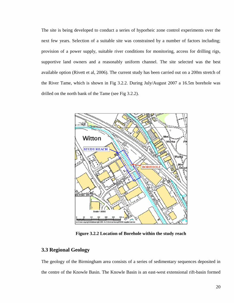
The site is being developed to conduct a series of hyporheic zone control experiments over the

next few years. Selection of a suitable site was constrained by a number of factors including;

provision of a power supply, suitable river conditions for monitoring, access for drilling rigs,

supportive land owners and a reasonably uniform channel. The site selected was the best

available option (Rivett et al, 2006). The current study has been carried out on a 200m stretch of

the River Tame, which is shown in Fig 3.2.2. During July/August 2007 a 16.5m borehole was

drilled on the north bank of the Tame (see Fig 3.2.2).

Figure 3.2.2 Location of Borehole within the study reach

3.3 Regional Geology

The geology of the Birmingham area consists of a series of sedimentary sequences deposited in

the centre of the Knowle Basin. The Knowle Basin is an east-west extensional rift-basin formed

21

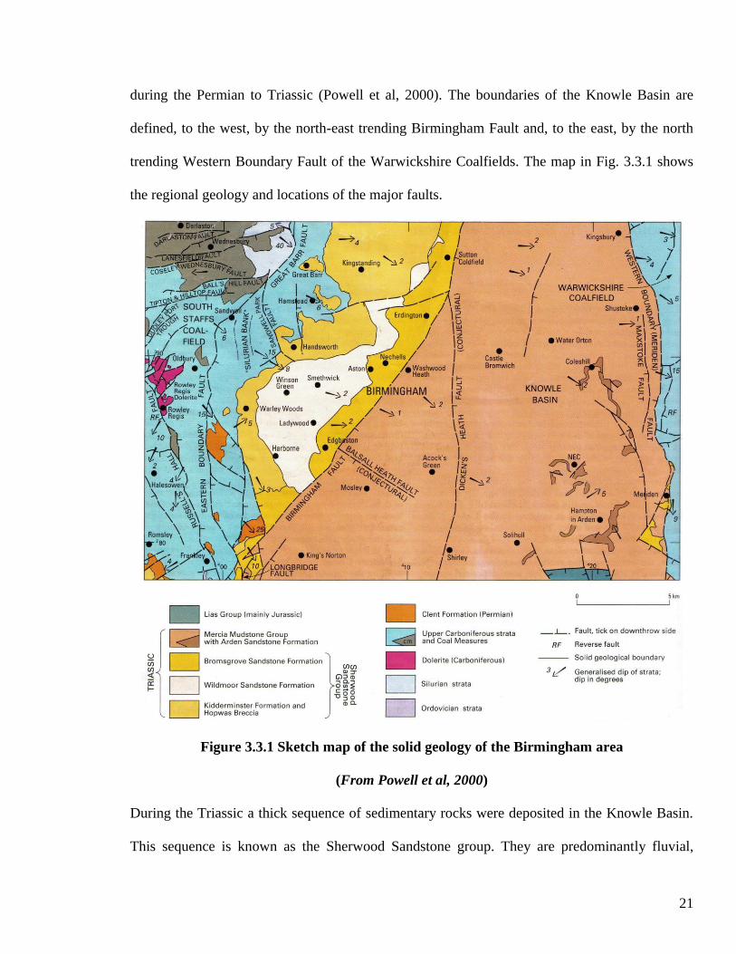
during the Permian to Triassic (Powell et al, 2000). The boundaries of the Knowle Basin are

defined, to the west, by the north-east trending Birmingham Fault and, to the east, by the north

trending Western Boundary Fault of the Warwickshire Coalfields. The map in Fig. 3.3.1 shows

the regional geology and locations of the major faults.

Figure 3.3.1 Sketch map of the solid geology of the Birmingham area

(From Powell et al, 2000)

During the Triassic a thick sequence of sedimentary rocks were deposited in the Knowle Basin.

This sequence is known as the Sherwood Sandstone group. They are predominantly fluvial,

22

continental and lacustrine sediments deposited in an arid to semi-arid climate. The Sherwood

Sandstone Group is overlain by the Mercia Mudstone Group, a series of red-bed mudstones and

siltstones deposited under lacustrine and fluvial conditions (Powell et al, 2000). The stratigraphy

of the Triassic sequence is shown in Table 3.3.1. The bedrock in the area is generally covered by

fluvial and glacial drift deposits which range in thickness from 1 to 40m.

Table 3.3.1 Stratigraphic sequence of the Triassic and Lower Jurassic in the region

(adapted from Powell et al, 2000)

3.3.1 Sherwood Sandstone Group

The base of the Triassic succession is defined locally by the Hopwas Breccia. This is overlain by

the Sherwood Sandstone Group, which comprises, in upward sequence, the Kidderminster

23

Formation, the Wildmoor Sandstone Formation and the Bromsgrove Sandstone Formation. The

Sherwood Sandstone Group varies in thickness across the region; generally it is up to 200m thick

although there is geophysical evidence suggesting a minimum thickness of about 625m in the

Knowle Basin (Powell et al, 2000).

Kidderminster Formation

The Kidderminster Formation consists of red-brown pebble conglomerate, pebbly sandstone and

medium- to coarse-grained, cross-bedded sandstone with intermittent, thin mudstone beds.

Generally the formation is weakly cemented and friable, however harder calcite cemented beds

are present locally (Powell et al, 2000). The formation crops out sporadically to the north-west of

the Birmingham Fault. It is thought that the formation was deposited as part of a major,

northward flowing, braided river system (Ellis, 2002). The formation has proved to be up to

119m thick in the central Birmingham area, and appears to thin out to the southeast as it

approaches the Birmingham Fault (Powell et al, 2000).

Wildmoor Sandstone Formation

The boundary between the Wildmoor Sandstone Formation and the Kidderminster Formation is

gradational. The Wildmoor Sandstone Formation consists of finer grained, micaceous soft

sandstone, which is orange-red in colour, and thin, red-brown and grey-green mudstone layers

(Powell et al, 2000). The formation is poorly cemented. Low-angle, planar cross-bedding

indicates fluvial deposition. It is thought that the formation was deposited by ephemeral streams

with some aeolian deposition (Ellis, 2002). There are few outcrops of the Wildmoor Sandstone

24

Formation in the region. Borehole data suggests that the formation is 30-86m thick to the north-

west of the Birmingham Fault and 7-40m thick to the south-east (Powell et al, 2000).

Bromsgrove Sandstone Formation

The Bromsgrove Sandstone Formation lies unconformably on the Wildmoor Sandstone

Formation and Kidderminster Formation. The unconformity represents a period of uplift and

erosion (Powell et al, 2000).The formation is composed of a series of upward fining sequences

from sandstone to mudstone. The sequence is made up of red-brown medium- to coarse-grained,

sub-angular arkosic sandstone, which locally contains pebble conglomerate beds, interbedded

with thin, red mudstone and siltstone layers. Deposition of the formation occurred in mature,

meandering river systems. To the south-east of the Birmingham Fault the formation is 84-180m

thick (Powell et al, 2000). The boundary with the overlying Mercia Mudstone Group is typically

gradational.

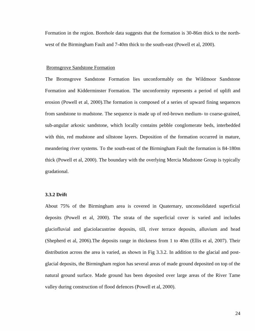
3.3.2 Drift

About 75% of the Birmingham area is covered in Quaternary, unconsolidated superficial

deposits (Powell et al, 2000). The strata of the superficial cover is varied and includes

glaciofluvial and glaciolacustrine deposits, till, river terrace deposits, alluvium and head

(Shepherd et al, 2006).The deposits range in thickness from 1 to 40m (Ellis et al, 2007). Their

distribution across the area is varied, as shown in Fig 3.3.2. In addition to the glacial and post-

glacial deposits, the Birmingham region has several areas of made ground deposited on top of the

natural ground surface. Made ground has been deposited over large areas of the River Tame

valley during construction of flood defences (Powell et al, 2000).

25

Figure 3.3.2 Regional drift map of Birmingham and surrounding area

3.4 Regional Hydrogeology

The Sherwood Sandstone Group forms the main aquifer system in the region, and is locally

known as the Birmingham aquifer. The eroded surface of the Carboniferous below the Sherwood

Sandstone is believed to represent the aquifer base. Regionally the aquifer is both confined and

unconfined. To the northwest of the Birmingham fault the aquifer is unconfined (Shepherd et al,

26

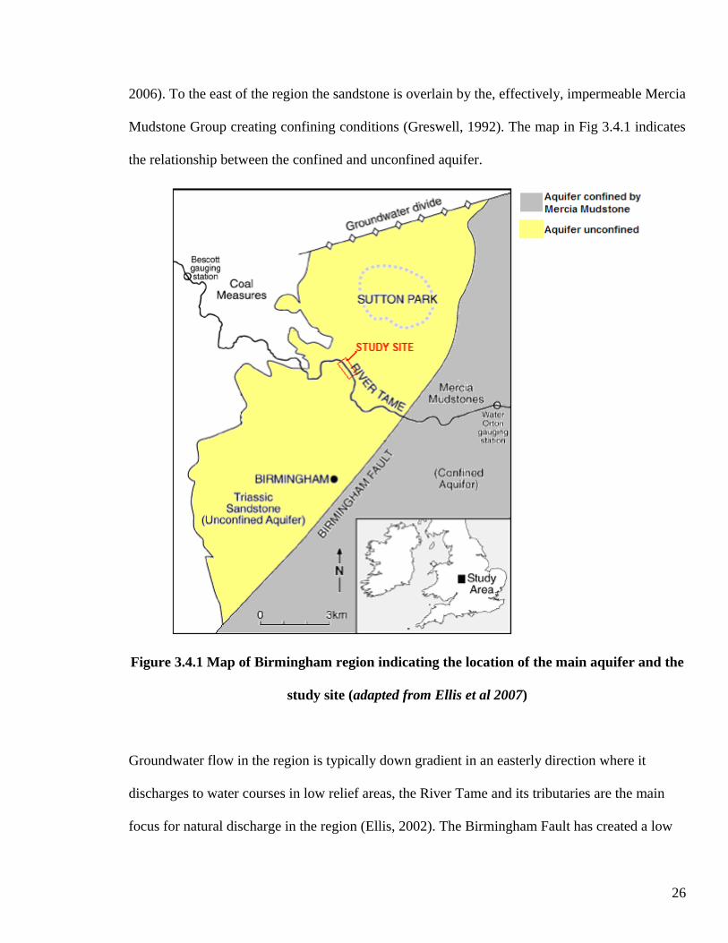
2006). To the east of the region the sandstone is overlain by the, effectively, impermeable Mercia

Mudstone Group creating confining conditions (Greswell, 1992). The map in Fig 3.4.1 indicates

the relationship between the confined and unconfined aquifer.

Figure 3.4.1 Map of Birmingham region indicating the location of the main aquifer and the

study site (adapted from Ellis et al 2007)

Groundwater flow in the region is typically down gradient in an easterly direction where it

discharges to water courses in low relief areas, the River Tame and its tributaries are the main

focus for natural discharge in the region (Ellis, 2002). The Birmingham Fault has created a low

27

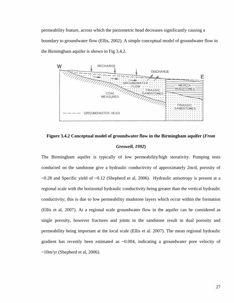
permeability feature, across which the piezometric head decreases significantly causing a

boundary to groundwater flow (Ellis, 2002). A simple conceptual model of groundwater flow in

the Birmingham aquifer is shown in Fig 3.4.2.

Figure 3.4.2 Conceptual model of groundwater flow in the Birmingham aquifer (From

Greswell, 1992)

The Birmingham aquifer is typically of low permeability/high storativity. Pumping tests

conducted on the sandstone give a hydraulic conductivity of approximately 2m/d, porosity of

~0.28 and Specific yield of ~0.12 (Shepherd et al, 2006). Hydraulic anisotropy is present at a

regional scale with the horizontal hydraulic conductivity being greater than the vertical hydraulic

conductivity; this is due to low permeability mudstone layers which occur within the formation

(Ellis et al, 2007). At a regional scale groundwater flow in the aquifer can be considered as

single porosity, however fractures and joints in the sandstone result in dual porosity and

permeability being important at the local scale (Ellis et al. 2007). The mean regional hydraulic

gradient has recently been estimated as ~0.004, indicating a groundwater pore velocity of

~10m/yr (Shepherd et al, 2006).

28

Recharge to the aquifer system is greatly influenced by the distribution and thickness of

superficial drift deposits that cover the region (Powell et al, 2000). The sands and gravels

present in the region potentially have high hydraulic conductivities of 10 – 30 m/d, and high

storage (Ellis et al, 2007). The average annual rainfall is non-uniform across the region, with

approximately 800mm in the south-west and 650mm in the north-east (Powell et al, 2000). Run-

off in the area is high due to widespread urban land use resulting in a low recharge from

precipitation, estimated at 130mm/yr (Shepherd et al, 2006). However significant recharge to the

aquifer is caused by leakage from sewers and water mains, and seepage from the extensive canal

network, estimated as 600mm/yr (Ellis, 2002).

Historically groundwater abstractions in the region have occurred for over 150 years,

predominantly for industrial purposes (Shepherd et al, 2006). Abstractions peaked in the 1950s

with over 60Ml/d, this has since steadily declined with the reduction in industrial demand to the

present day abstractions of approximately 13Ml/d (Ellis et al, 2007). The decline in groundwater

abstractions over the past 50 years has resulted in a significant rise in water levels (Powell et al,

2000).

3.5 Local Geology

The study site is located approximately 1km northwest of the Birmingham fault. The geological

map shown in Fig 3.5.1 indicates that the site rests on the Kidderminster Formation, which is

part of the Sherwood Sandstone group. Various borehole logs from the surrounding area indicate

that the sandstone is 71 – 80m thick, with a median thickness of ~76m (Lydon, 2006). The base

of the sandstone rests disconformably on the Hopwas Breccia.

29

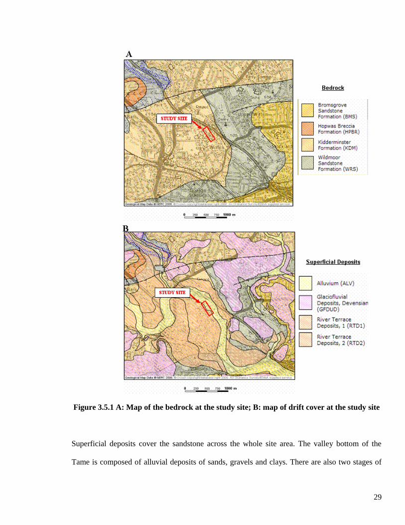
Figure 3.5.1 A: Map of the bedrock at the study site; B: map of drift cover at the study site

Superficial deposits cover the sandstone across the whole site area. The valley bottom of the

Tame is composed of alluvial deposits of sands, gravels and clays. There are also two stages of

30

river terrace deposition, which predate the recent alluvial deposits. Fig 3.5.1 shows the

complexity of the drift cover in the area. Glaciofluvial deposits also cover the area. The borehole

drilled on site indicated that superficial cover on the north bank of the River Tame was

approximately 8.5m thick, with the alluvium composed of sand and gravel. A 2m layer of made

ground covers the drift.

3.6 Local Hydrogeology

The study site is situated on an unconfined part of the Birmingham aquifer. Groundwater flow in

the area is typically from west to east. A numerical model constructed by Ellis (2002) indicates

that in close proximity to the River Tame groundwater flows towards the river, as shown in Fig

3.6.1. Head measurements, from piezometers installed in the riverbed during field work, and

from previous studies, indicate that the River Tame is gaining along the entire study reach, with a

median hydraulic gradient of 0.0875.

Figure 3.6.1 Distribution of groundwater head in the study area (from Ellis 2002)

31

3.7 Hydrology

The catchment area drained by the Tame is 408 km2 (Ellis et al, 2007). The river is described as

extensively modified; it bares little resemblance to its natural form of a meandering braided river

system. Flood defence work carried out along the river has resulted in the river being

straightened along many sections and river banks being strengthened, this includes the study site

as shown in Fig 3.7.1, the base of the channel has remained natural and unlined.

Figure 3.7.1 Study site looking upstream from the Gavin Way Bridge, the river has been

straightened as part of flood defence work carried out in the area.

In the study area the river is typically 8-12m wide, 0.2-2m deep and has an average dry weather

flow velocity of 0.1-0.8 m/s (Ellis 2002). Over the study section the river stage maintains a

comparatively constant shallow gradient of 0.0013. The riverbed is composed of a range of

materials from sub angular cobbles to gravel, sand and silt. During the summer months weed

32

growth in the river is substantial and is thought to affect the hydrological regime by reducing

flow velocities (Ellis, 2002).

33

Chapter 4. Data Collection

4.1 Introduction

The project area used for this study consisted of a 200m stretch of the River Tame to the north of

the Holford industrial estate. This chapter looks at the methods used for collecting data in the

field to use for subsequent analysis and modelling. A network of riverbed piezometers were

installed for the study and these, along with a small scale pump test conducted on the borehole

on site, were used as the main sources for data. The installation of piezometers and data

collection was carried out during August 2007, following delays in accessing the river (due to

high water levels following a prolonged period of rain) and gaining permissions to access the

site.

The aims of the fieldwork applied to the study area were:

To identify the hydraulic gradients below the river bed.

Obtain hydraulic conductivity (K) estimates of river bed sediments from falling head

piezometer tests.

Obtain hydraulic conductivity (K) estimates of the sandstone aquifer from a small scale

pump test.

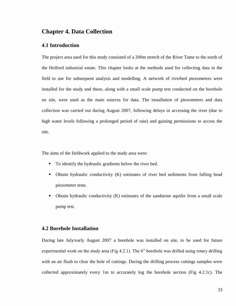
4.2 Borehole Installation

During late July/early August 2007 a borehole was installed on site, to be used for future

experimental work on the study area (Fig 4.2.1). The 6” borehole was drilled using rotary drilling

with an air flush to clear the hole of cuttings. During the drilling process cuttings samples were

collected approximately every 1m to accurately log the borehole section (Fig 4.2.1c). The

34

borehole was drilled to a depth of 16.5m. The entire length of the borehole was cased, with 6m

of slotted casing at the base of the borehole to permit water to enter the borehole from the

sandstone aquifer.

Figure 4.2.1 Installation of borehole on the north bank of the River Tame; A, Drill bits and

casing used; B, Drilling the borehole; C, Borehole log indicating depth below ground level

of different sediment layers and the depths of plain and slotted casing

35

4.3 Pump Test

A groundwater sample was required from the borehole for chemical analysis as part of the main

research study on the site. A submersible pump was used to remove enough well-bore volumes

to retrieve a suitable water sample. The opportunity was taken to measure the drawdown in the

well during pumping and recovery to allow an estimate of the sandstone hydraulic conductivity

to be calculated.

Collecting accurate drawdown data from a pumping test will depend on the following:

Maintaining a constant yield during the test

Measuring the drawdown in the pumping well carefully

Taking drawdown readings at appropriate intervals

Recording data from both the pumping and recovery periods

A small generator was used to power the pump. Pumping was at a constant discharge of 0.67 l/s.

The discharge was measured by observing the time taken to fill a 10 litre bucket. This is a

practical way of measuring discharge at low pumping rates (Driscoll, 1995).

Water level measurements were only made in the pumping borehole. Ideally, measurements from

nearby piezometers are needed to get accurate data from a pumping test, however there were

none available at the time the test was carried out. The accuracy of data taken from single-well

pump tests is usually less reliable because of turbulence created by the pump, however the data

can still be used to give a useful estimate of the aquifer transmissivity.

36

Measurements were made using a dip meter which provided a noise when the probe was

immersed in water. Prior to pumping the static water level in the borehole was measured. All

measurements were taken relative to the top of the well casing. As early test data provide the

most important information when conducting a pumping test, on commencement of pumping

measurements of the water level were recorded to the nearest 10 seconds. During the pumping,

the pump became jammed (possibly with leaves and debris that were sitting in the borehole), to

resolve this issue the pump was switched on and off a couple of times to clear the blockage and

continue pumping at a constant rate. This resulted in water level data only being accurately

measured for the first 3 minutes of pumping. Following 1 hour of continuous pumping the water

level in the borehole was at a relatively steady state. The pump was switched off and the

recovery was monitored. During the first four minutes of recovery the water level was recorded

every 10 seconds, and then for every 30 seconds until the water level had recovered to its

original level in just over 10 minutes.

4.4 Analysis of Pump Test Data

Pump test data was analysed using the Cooper-Jacob (1946) method which can be applied to

single-well pump tests to estimate the aquifer transmissivity. The drawdown observed during the

pump test was calculated by subtracting the water level measurements from the original static

water level measured prior to pumping. The pumping and recovery data were analysed

separately.

Data obtained during the discharge period of the pump test were analysed by constructing a

semi-log plot of observed values of drawdown in the pumping well (sw) versus the time (t) on the

37

logarithmic scale. A best-fit straight line was drawn through the data points, and the slope of the

line calculated, i.e. the drawdown difference ∆sw per log cycle of time. Using the Cooper-Jacob

method the transmissivity is calculated from:

ws

QKD

4

30.2

Where:

KD is the transmissivity (K is hydraulic conductivity, D is saturated aquifer thickness)

Q is well discharge

Using the relationship that the transmissivity is equal to the hydraulic conductivity multiplied by

the saturated aquifer thickness, an estimate of the hydraulic conductivity for the sandstone

aquifer could be made. As the borehole only partially penetrated the aquifer, the length of the

slotted casing (6m) was used to estimate the hydraulic conductivity; this was appropriate because

the borehole only penetrated 10% of the aquifer thickness (assuming it is 100m thick) and has a

low transmissivity (Halford et al, 2006).

Data obtained from the recovery period of the test was analysed by constructing a semi-log plot

of residual drawdown (s’w) versus the ratio between the time since the start of pumping and time

since the end of pumping (t/t’) on the logarithmic scale. A best fit straight line was drawn

through the data points, and the slope of the line calculated (∆s’w). The transmissivity is

calculated using:

ws

QKD

'4

30.2

38

The transmissivity calculated for the recovery period was used to estimate the hydraulic

conductivity using the same method as described above for the discharge period.

4.5 Construction of Riverbed Mini Drive Point Piezometers (MDP’s)

In order to identify the hydraulic gradients between the river bed sediments and the river, mini

drive point piezometers (MDP’s) were constructed and installed at selected profiles within the

river bed. A series of multi-level chemical sampling tubes were attached to the MDP in order to

enable chemical water samples to be taken during future experimental work at the site. The

MDP’s were required to cover a depth of up to 1m below the river bed, in order to full penetrate

the hyporheic zone which is thought to be up to 0.6m deep in this stretch of the river (Ellis,

2002).

The MDP’s were constructed using flexible, high density polyethylene tubing (HDPE), 100

micron nylon mesh, stainless steel bolts, washers and wire. The HDPE tubing had an internal

diameter of 10mm and an outer diameter of 13mm. Chemical sampling tubes were required at

10cm intervals over a 1m depth of the river bed, whereas half of the MDP’s were required to

have an open section at 1m depth and the other half at 0.5m depth. To allow for this all the

MDP’s were designed to be installed at a depth of 1m below the river bed, with the position of

the open section of the MDP modified accordingly, the basic design is shown in Fig 4.5.1. The

HDPE tubing was cut into 2m lengths. For the 1m MDP’s open section a 4mm drill bit was used

to drill holes through the tubing placed 1cm apart longitudinally to cover a 10cm length at the

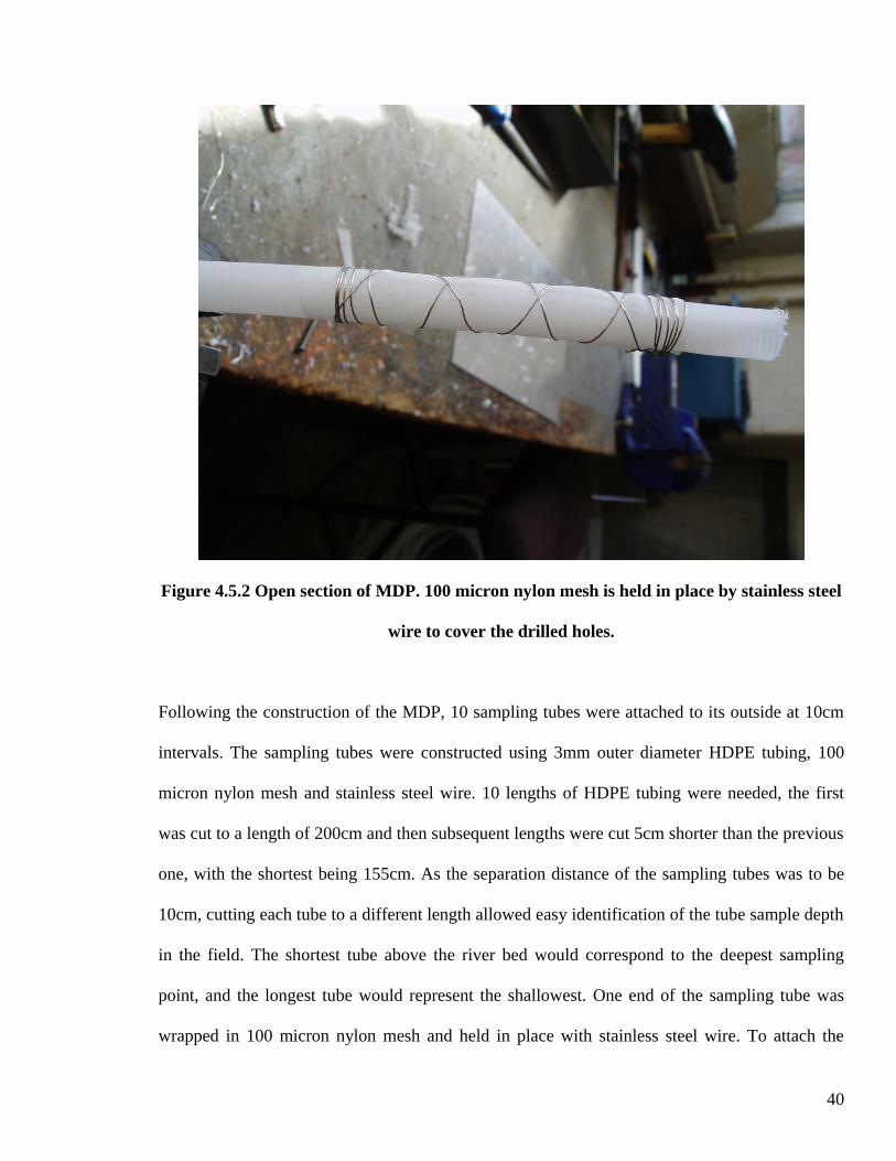
end of the tube. The drilled section of tube was then covered in 1 layer of 100 micron nylon

mesh which was secured with thin, stainless steel wire (Fig 4.5.2). The nylon mesh acts as a

39

screen to prevent clogging of the open section. For the 0.5m MDP’s the open section was

constructed in the same way however it was positioned 0.5m from the end of the tubing.

Figure 4.5.1 Schematic diagram of MDP design. The 1m MDP (on the left) is inserted to a

depth of 1m below the stream bed, the open section is at a depth of 1m, the position of the

multi-level samplers are placed at 10cm intervals over a depth of 1m. The 0.5m MDP (on

the right) is inserted to a depth of 1m below the stream bed, the open section is at a depth

of 0.5m, multi-level samplers are placed at 10cm intervals over a depth of 1m.

40

Figure 4.5.2 Open section of MDP. 100 micron nylon mesh is held in place by stainless steel

wire to cover the drilled holes.

Following the construction of the MDP, 10 sampling tubes were attached to its outside at 10cm

intervals. The sampling tubes were constructed using 3mm outer diameter HDPE tubing, 100

micron nylon mesh and stainless steel wire. 10 lengths of HDPE tubing were needed, the first

was cut to a length of 200cm and then subsequent lengths were cut 5cm shorter than the previous

one, with the shortest being 155cm. As the separation distance of the sampling tubes was to be

10cm, cutting each tube to a different length allowed easy identification of the tube sample depth

in the field. The shortest tube above the river bed would correspond to the deepest sampling

point, and the longest tube would represent the shallowest. One end of the sampling tube was

wrapped in 100 micron nylon mesh and held in place with stainless steel wire. To attach the

41

sampling tubes to the MDP, 10cm intervals from the end of the MDP tube were measured; a

single length of stainless steel wire was wrapped around the MDP, and then the first sampling

tube (1m depth) to attach it securely to the MDP. The wire was continually wrapped around the

MDP to ensure that the sampling tube would remain in place, for every 10cm interval another

sampling tube was attached until all 10 were securely held in place (Fig 4.5.3). Once the

sampling tubes were attached, brass screws were inserted into the open end to prevent algae

growth and cross contamination of sample horizons. Fig 4.5.4 shows the completed multi-level,

mini drive point piezometer.

Figure 4.5.3 Design and attachment of sampling tube to the MDP.

42

Figure 4.5.4 Completed multi-level, mini drive point piezometer

4.6 Installation of MDP’s

The installation of the piezometers required a hollow 3m steel pole and a 15kg fence post driver.

The piezometer was inserted inside the steel pole with care taken to ensure the sampling tubes

did not slip out of place. Once the piezometer was inside the steel pole two washers and a

stainless steel bolt were attached to the end of the MDP tube, as the washers and bolt head had a

larger diameter than the steel pole they would prevent slippage of the piezometer during

installation and act as the drive point. The steel pole was driven by hand, using the fence post

driver, into the river bed to the required depth which was marked on the outside of the steel pole

43

(Fig4.6.1). Once the steel pole had been driven to the required depth, it was removed allowing

the sediments to collapse naturally around the piezometer and hold it in place.

Figure 4.6.1 Installation of piezometer, a fence driver post is used to drive the steel pole to

the required depth

The variability of sand and gravel bed sediments in the Tame provided varying levels of

resistance to installation of the piezometers. In many cases it was not possible to drive the

piezometers down to the required 1m depth. In these cases the piezometer was driven as far as

possible. The length of the MDP tubing remaining above the river bed was measured for each

piezometer so its exact depth could be calculated.

44

Particular problems were encountered during installation of the MDP’s which had an open

section at 0.5m along its length. In some cases these piezometers were driven down to 0.5m or

less resulting in the open section protruding above the river bed surface; some of the sampling

tubes were below the river bed. For these locations simple MDP’s were constructed, with the

open section at the end of the HDPE tubing. Their construction used the same method as

described in section 4.5 however no chemical sampling tubes were attached to these piezometers,

which were then installed next to the previously installed multi-level MDP’s.

4.7 Hydraulic Gradient

Calculating the hydraulic gradients between the groundwater and the river has been carried out to

establish the direction of water movement below the river bed i.e. gaining or losing. To calculate

the hydraulic gradient, groundwater head measurements were taken from the MDP’s.

The piezometers were held upright and the water level was given time to equilibrate with

atmospheric pressure. Due to the relatively transparent nature of the tubing used in the

construction of the MDP’s, the groundwater head level could be measured directly using a tape

measure. This was possible because the piezometers had been newly installed. However, even

after only a week of installation, there was significant algae growth on some of the piezometers

which made it difficult to observe the water level. This was resolved by cleaning the algae off the

piezometer tubes using a metal scouring pad. The head levels in the piezometers were measured

as height above the river water level, which was used as the datum.

45

The groundwater head level and known depth of the piezometer could then be used to calculate

the hydraulic gradient as follows:

i = h2 – h1

L

Where:

i is the hydraulic gradient

h1 is the river water level (datum point = 0m)

h2 is the water level in the piezometer

L is the depth of the open section of the piezometer in the river bed

4.8 Falling Head Tests

Falling head tests were conducted on all the MDP’s to calculate estimates of the hydraulic

conductivity of the river bed sediments. A falling head test involves the application of a greater

hydraulic pressure in the piezometer, and measuring the rate of change in the pressure as it

equilibrates to the natural conditions. The change in hydraulic pressure was done, in this case, by

introducing water into the piezometer tube. The rate of change in pressure was represented by

measuring the rate of change of the water level in the piezometer.

To conduct the test the open end of the piezometer tube was held under the river water level and

allowed to fill with river water, making sure there was no air left in the tube. By placing a thumb

over the end of the tube, it could be lifted upright out of the water and the hydraulic pressure

could be maintained. The piezometer was held next to a wooden board which had 10cm intervals

46

marked onto it (Fig 4.8.1). The thumb was removed from the end of the tube and the timer was

started. As the water level dropped the time taken to reach each 10cm interval was noted until the

water level had reached a steady state. This process was repeated 3 times for each piezometer to

ensure consistency of the data.

Figure 4.8.1 Falling head test on piezometer. 10cm intervals were marked on the wooden

board held next to the piezometer to allow the change in head level to be easily measured.

4.9 Analysis of Falling Head Test Data

The analysis of falling head test data taken from the piezometers was done using the Hvorslev

(1951) method. Hvorslev found that water levels will return to their normal static level at an

exponential rate, with the time taken dependent on the hydraulic conductivity of the porous

47

material (Hiscock, 2005). The calculation of hydraulic conductivity can be made using the

following equation:

K = r2 loge (L/R)

2LT0

Where:

K is the hydraulic conductivity

r is the radius of the well casing

L is the length of the piezometer open section

R is the radius of the well screen

T0 is the time taken for the water level to fall to 37% of the initial change

(see Fig 4.9.1a)

The calculation of hydraulic conductivity can be found provided the length, L, is greater than

eight times the radius of the well screen, R.

A semi-log plot of the ratio, h/h0 (where, h is the height of the water level above the static water

level, and h0 is the initial height of the water level above the static level at the start of the test)

versus time, t, was made and a straight line was fitted to the data, from which T0 could be found

(see Fig 4.9.1b). The T0 value could then be used in the above equation and the hydraulic

conductivity calculated.

48

Figure 4.9.1 Hvorslev piezometer test; (a) piezometer geometry; (b) graphical method for

analysis of T0 (From Hiscock, 2005)

A hydraulic conductivity value was calculated for each of the three falling head tests carried out

on an individual piezometer. The arithmetic mean of the three values was then taken to give a

hydraulic conductivity estimate for the river bed sediments surrounding that piezometer.

49

Chapter 5. Fieldwork Results

5.1 Introduction

The collection and analysis of data collected in the field are described in the previous chapter.

This chapter presents the results, which aimed to define the hydraulic properties of the sandstone

aquifer and river bed sediments, for use in subsequent modelling.

5.2 Pump Test

The full list of results taken from the pumping test are given in Appendix 1. The graphs of

drawdown (s) versus time (t) for the discharge period of the test and for residual drawdown (s’)

versus t/t’ are shown in Fig 5.2.1 and 5.2.2 respectively.

y = x - 1.47

0

0.5

1

1.5

2

2.5

1 1.2 1.4 1.6 1.8 2 2.2 2.4 2.6

Log t (days)

s (

m)

..

Figure 5.2.1 Discharge period of pump test

50

y = 1.0526x - 0.9019

0

0.4

0.8

1.2

1.6

2

0.5 0.7 0.9 1.1 1.3 1.5 1.7 1.9 2.1 2.3 2.5

Log t/t' (days)

s' (m

) .

Figure 5.2.2 Recovery period of pump test

The calculated transmissivity and estimates of the hydraulic conductivity are given in Table 5.2.1

below.

Test Period Calculated T (m2/d) Estimated K (m/d)

Discharge 10.61 1.76

Recovery 10.09 1.68

Table 5.2.1 Calculated transmissivity and estimated hydraulic conductivity values from

discharge and recovery periods of the pump test.

The two estimates for the hydraulic conductivity of the sandstone aquifer show good

consistency. The arithmetic mean hydraulic conductivity is 1.72 m/d. This result is consistent

with previous estimates of the hydraulic conductivity of the Kidderminster Sandstone, which is

given as 2 m/d by Shepherd et al (2006). As the pump test had only been monitored at the

51

pumping borehole, transmissivity is the only hydraulic property for the sandstone which could be

calculated.

5.3 Piezometer Installation

In total 20 piezometers were installed in the river bed at 8 lateral profiles along the study reach.

The locations of the piezometers are shown in Fig 5.3.1.

Figure 5.3.1 Map of study site indicating the location of all the piezometers installed on site

for this project

52

The sequence in which the piezometers are referenced is as follows. First the location of the

piezometer (P) in relation to the borehole installed on site is referenced; -, if it is upstream of the

borehole, +, if it is downstream of the borehole, along with its distance in metres from the

borehole, e.g. P-050, refers to a piezometer 50 m upstream from the borehole. Finally the

position of the piezometer in the river is noted; 1, if it is closest to the north river bank; 2, if it is

in the centre of the river; 3, if it is closest to the south river bank. The locations of the

piezometers can be easily found in the field as a yellow of spot, painted onto the rocks on the

south river bank, indicates the position of each piezometer profile.

The installation depths of the MDP’s ranged from 0.02 m to 1m. They were driven on average to

0.51 m. Penetration of the bed sediment became increasingly difficult below this depth due to the

nature of the sediment strata. A full list of the depths of each piezometer is given in Appendix 3.

The positioning of the piezometers across the channel and at varying depths was done to assess

the heterogeneities within the river bed sediments. The positioning of an equal number of

piezometers (and similar pattern) either side of the borehole was done so that the influence of

pump tests, taking place in the future, on the groundwater levels within the river bed could be

accurately monitored.

5.4 Groundwater Head Measurements

The groundwater level in each piezometer was measured as height above the river water level. It

would be expected that in a homogeneous medium, the groundwater head would increase with

depth. However a plot (shown in Fig 5.4.1) of the piezometer groundwater head measurements

53

versus their depth produced a large scatter of results which did not follow this rule and indicated

the heterogeneous nature of the river bed sediments

0

0.02

0.04

0.06

0.08

0.1

0.12

0 0.2 0.4 0.6 0.8 1 1.2Depth (m)

Head

(m

) .

P-090

P-050

P-022

P-004

P+005

P+023

P+070

P+110

Figure 5.4.1 Plot of groundwater head versus depth, indicates the heterogeneous nature of

the river bed sediments. Individual piezometer profiles are picked out.

The plot shown in Fig 5.4.1 does, however, show some correlation between groundwater head

and depth if individual piezometer profiles are picked out. Profiles P-004, P+100 and P-022 all

indicate that the groundwater head is increasing with depth, suggesting that there may be less

vertical heterogeneity in these areas. The profiles for P+005 and P-090 do not show this

54

relationship, with the groundwater head appearing to decrease with depth, indicating large

heterogeneities within the river bed sediments.

5.5 Hydraulic Gradients

Groundwater head measurements were taken for all the piezometers, and this value along with

the known depth of the piezometer was used to calculate the hydraulic gradient of the river. The

results are given in Table 5.5.1.

Piezometer Depth (m) Groundwater Head (m.a.d) Calculated Hydraulic Gradient

P-090-1 0.45 0.025 0.0556

P-090-2 0.37 0.05 0.1351

P-050-1 0.5 0.05 0.1

P-050-2 0.5 0 0

P-022-1 0.55 unable to measure ?

P-022-2 0.48 0.035 0.0729

P-022-3 0.6 0.11 0.1833

P-004-1 0.17 0 0

P-004-2 0.62 0.05 0.0806

P-004-3 0.15 0.02 0.1333

P+005-1 0.46 0.09 0.1957

P+005-2 0.42 0.1 0.2381

P+005-3 0.74 0.09 0.1216

P+023-1 0.24 0 0

P+023-2 0.8 0.07 0.0875

P+023-3 0.32 0 0

P+070-1 0.47 0.01 0.0213

P+070-2 1 0.04 0.04

P+110-1 0.92 0.06 0.0652

P+110-2 0.43 0.01 0.0233

Table 5.5.1 Calculated hydraulic gradients for each piezometer. Groundwater head

measured as height above datum (river water level).

55

The results give a range of hydraulic gradients from 0 to 0.2381, with an average gradient of

0.1036. This indicates that along much of the study reach the river is gaining. P-050-2, P-004-1,

P+023-1 and P+023-3 indicated a head level equal to that of the river indicating neutral

conditions, i.e. the river is neither gaining nor losing at these points.

The range of hydraulic gradients observed indicates the heterogeneous nature of the streambed.

These heterogeneities are particularly apparent by comparing the results of piezometers from a

single profile. For example piezometer 1 in profile P-90 has a hydraulic gradient of 0.0556,

which is less than half that observed in piezometer 2 in the same profile which has a gradient of

0.1351. The variations indicate that the stream bed is heterogeneous both vertically and laterally.

No calculation of the hydraulic gradient could be made for P-022-1. This was because a

measurement of the groundwater head could not be made in the field; this is discussed further in

section 5.6.

5.6 Falling Head Tests

Falling Head tests were conducted in 17 of the 20 piezometers installed during the fieldwork.

Falling head tests could not be carried out in P+070-1, P+070-2 and P+110-2, this was due to the

river water level being deeper in these area than expected during installation of the piezometers

resulting in the piezometer tube being too short to and sticking out no more than about 15cm

above the river surface. This meant that there was not a long enough section of piezometer tube

to conduct a falling head test in. Attempts were made to connect a longer piece of tubing onto the

56

end of the piezometers using plastic connectors and metal clamps, however this method was

unsuccessful.

The results of falling head tests in 5 of the riverbed piezometers failed or proved inconclusive

when tested. The tests on P-022-1 were recorded as having failed when no percolation of water

occurred through the open section. Several reasons may account for this type of failure. It is

likely to have been caused by either damage to the screened section during the installation

procedure or as a result of encountering very low permeability strata. The tests on P-050-2, P-

004-1, P+023-1 and P+023-3 proved inconclusive. As the groundwater level in these

piezometers was in equilibrium with the river level, there was no pressure difference between the

two, resulting in a falling head test being impossible to carry out. This may suggest that the

piezometer was in fact in hydraulic connection with the river rather than the groundwater in the

river bed sediments. This could possibly be due to damage caused during installation to the

piezometer and/or the removal and reorganisation of sediments within the river bed during

installation.

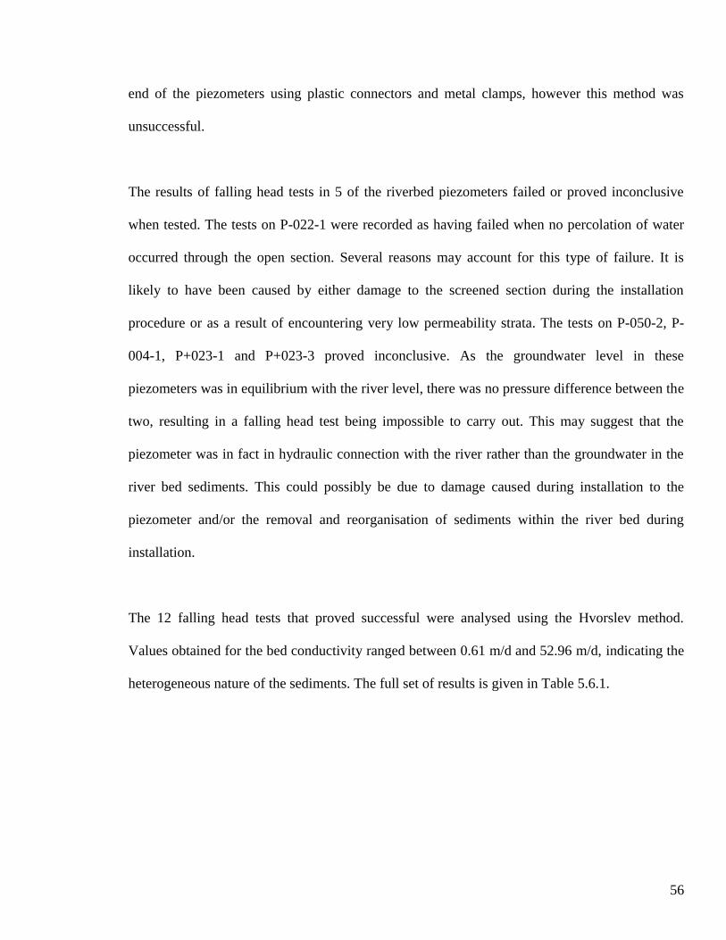
The 12 falling head tests that proved successful were analysed using the Hvorslev method.

Values obtained for the bed conductivity ranged between 0.61 m/d and 52.96 m/d, indicating the

heterogeneous nature of the sediments. The full set of results is given in Table 5.6.1.

57

Piezometer Depth (m) K (m/d)

P-090-1 0.45 9.31

P-090-2 0.37 6.32

P-050-1 0.5 2.09

P-050-2 0.5 ?

P-022-1 0.55 ?

P-022-2 0.48 6.54

P-022-3 0.6 0.61

P-004-1 0.17 ?

P-004-2 0.62 3.67

P-004-3 0.15 10.45

P+005-1 0.46 52.96

P+005-2 0.42 16.2

P+005-3 0.74 1.85

P+023-1 0.24 ?

P+023-2 0.8 12.58

P+023-3 0.32 ?

P+070-1 0.47 ?

P+070-2 1 ?

P+110-1 0.92 1.24

P+110-2 0.43 ?

Table 5.6.1 Hydraulic conductivity estimates from falling head test. ? indicates failed,

inconclusive or no test.

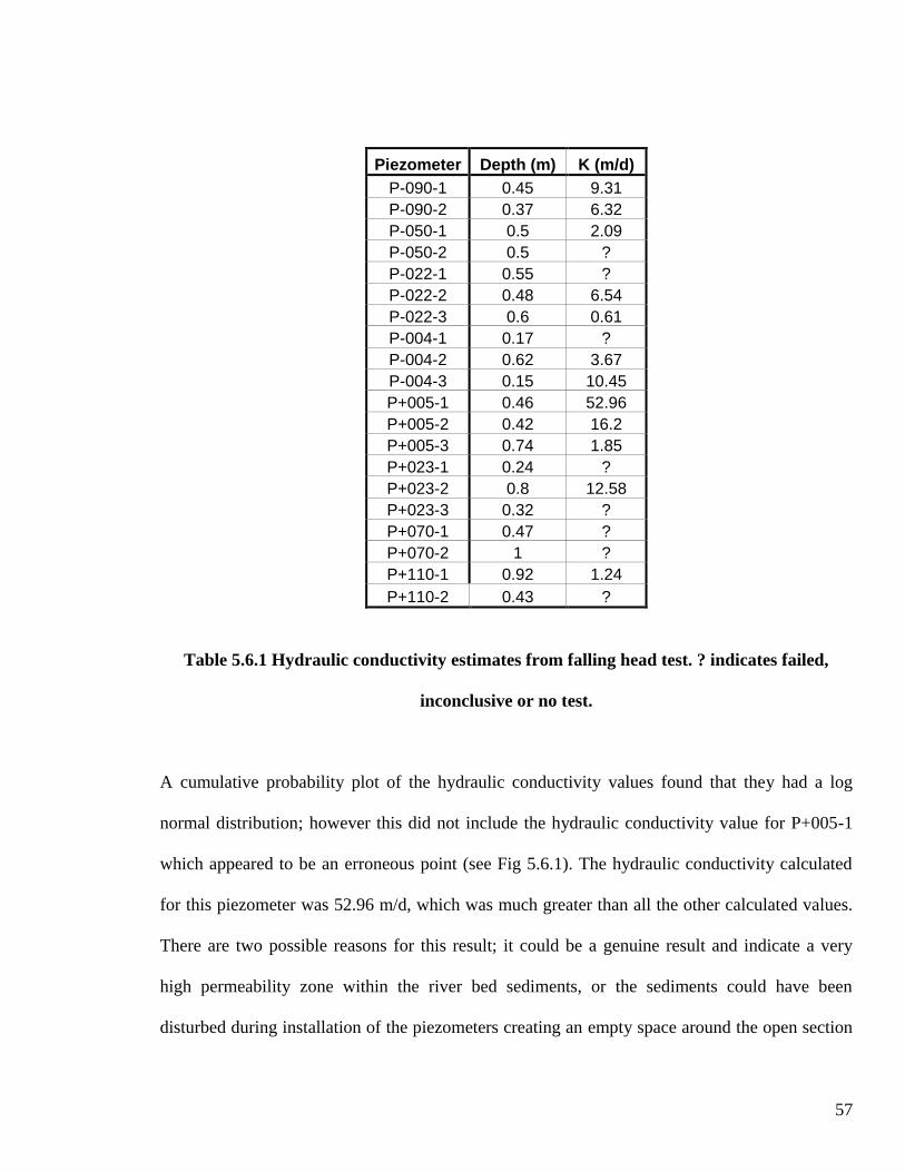
A cumulative probability plot of the hydraulic conductivity values found that they had a log

normal distribution; however this did not include the hydraulic conductivity value for P+005-1

which appeared to be an erroneous point (see Fig 5.6.1). The hydraulic conductivity calculated

for this piezometer was 52.96 m/d, which was much greater than all the other calculated values.

There are two possible reasons for this result; it could be a genuine result and indicate a very

high permeability zone within the river bed sediments, or the sediments could have been

disturbed during installation of the piezometers creating an empty space around the open section

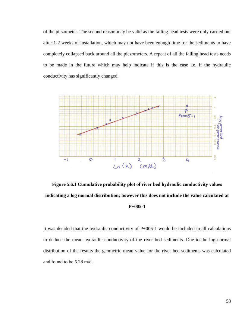
58

of the piezometer. The second reason may be valid as the falling head tests were only carried out

after 1-2 weeks of installation, which may not have been enough time for the sediments to have

completely collapsed back around all the piezometers. A repeat of all the falling head tests needs

to be made in the future which may help indicate if this is the case i.e. if the hydraulic

conductivity has significantly changed.

Figure 5.6.1 Cumulative probability plot of river bed hydraulic conductivity values

indicating a log normal distribution; however this does not include the value calculated at

P+005-1

It was decided that the hydraulic conductivity of P+005-1 would be included in all calculations

to deduce the mean hydraulic conductivity of the river bed sediments. Due to the log normal

distribution of the results the geometric mean value for the river bed sediments was calculated

and found to be 5.28 m/d.

59

The values obtained for the river bed hydraulic conductivity were then split into two categories,

those at 0m to 0.5m depth below the river bed and those at >0.5m to 1m below the river bed.

This was to assess the differences in values at varying depths.

Values obtained for the river bed hydraulic conductivity between 0m and 0.5m ranged between

2.09 m/d and 52.96 m/d, giving a geometric mean of 9.54 m/d. Values obtained for the river bed

hydraulic conductivity between 0.5m and 1m ranged between 0.61 m/d and 12.58 m/d, giving a

geometric mean of 2.30 m/d.

The range of hydraulic conductivity values observed between the individual piezometers

indicates the extremely heterogeneous nature of the river bed sediments. Low values of hydraulic

conductivity, such as 0.61 m/d calculated in P-022-3, could indicate low permeability zones, e.g.

clay lenses, within the sediments.

5.7 Conclusions

Estimates of hydraulic conductivity for the sandstone from pump test data, gave good results

which were comparable with literature values.

The geometric mean value for hydraulic conductivity (5.28 m/d) from falling head test analysis

is considered to provide a good estimate for the combined vertical and horizontal riverbed

hydraulic conductivity. A repeat of all the falling head tests needs to be made in the future to

allow the river bed sediments more time to settle out following the piezometer installation. New

piezometers may need to be installed to solve the problems encountered when attempting to

60

carry out some of the falling head tests, i.e. P-022-1 where the open section appears to be

blocked or damaged and longer piezometers installed in the locations where the current ones are

too short.

Overall the results shown for hydraulic conductivity, groundwater head and hydraulic gradients

support the theory that river bed sediments have a very heterogeneous nature. All the data sets

described in this chapter are given in the appendices.

61

Chapter 6. Modelling

6.1 Introduction

To analyse the effects of a proposed pump test on the study site a basic numerical model of the

aquifer system was created. The aim of the modelling work was to investigate:

the effect of pumping on the hydraulic gradients observed within the river bed

the sensitivity of both known and estimated hydraulic parameters applied to the model

The model could then be used to predict the expected response in the river bed piezometers for

future experiments on the site.

The basic model grid had been created by Dr. Veronique Durand; this model was used to apply

the hydraulic parameters established in the field and test its sensitivity. MODFLOW was the

code used in the modelling. MODFLOW uses a block-centred finite-difference approach to

simulating groundwater flow within an aquifer. The code was run using the software interface

Processing Modflow Pro (version 7.0.11), which allows for a large quantity of layers to be

modelled.

6.2 Basic Conceptual Model

A conceptual model of the groundwater flow system was established, using field and archive

data, to describe the aquifer geometry, the local boundary conditions and estimates of the

hydraulic parameters. To conceptualise the system some simplifications had to be made.

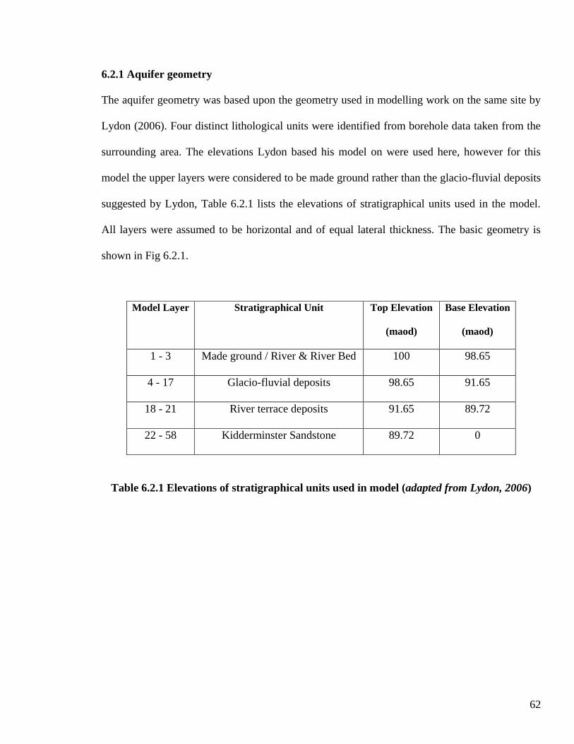
62

6.2.1 Aquifer geometry

The aquifer geometry was based upon the geometry used in modelling work on the same site by

Lydon (2006). Four distinct lithological units were identified from borehole data taken from the

surrounding area. The elevations Lydon based his model on were used here, however for this

model the upper layers were considered to be made ground rather than the glacio-fluvial deposits

suggested by Lydon, Table 6.2.1 lists the elevations of stratigraphical units used in the model.

All layers were assumed to be horizontal and of equal lateral thickness. The basic geometry is

shown in Fig 6.2.1.

Model Layer Stratigraphical Unit Top Elevation

(maod)

Base Elevation

(maod)

1 - 3 Made ground / River & River Bed 100 98.65

4 - 17 Glacio-fluvial deposits 98.65 91.65

18 - 21 River terrace deposits 91.65 89.72

22 - 58 Kidderminster Sandstone 89.72 0

Table 6.2.1 Elevations of stratigraphical units used in model (adapted from Lydon, 2006)

63

Figure 6.2.1 Basic geometry used in modelling (not to scale)

6.2.2 Boundary conditions/initial heads

Constant head boundaries were set parallel to the River Tame to the north east and south west

both had a value of 100 maod along their entire length (Fig 6.2.2). These boundaries were set far

enough away from the pumping borehole so that they would not influence it.

The River Tame was also modelled as a constant head boundary of 100 maod. Applying a

constant head boundary to act as the river ensured a constant supply of water from the river when

running the model. Initial heads across the model were set at 100 maod. Modelling the river and

initial head levels in this way was acceptable as the model was to be used to look at the change in

groundwater head below the river (i.e. drawdown), not the actual groundwater levels observed.

64

Figure 6.2.2 Position of constant head boundaries on model grid

6.2.3 Aquifer hydraulic parameters

The initial estimates of hydraulic parameters used in the model were taken from the fieldwork

results, and combined with literature values for the properties that were not measured in the field.

All hydraulic conductivity values were assumed to be isotropic. The initial values used in the

model are listed in Table 6.2.2. Values for the made ground were unknown, it was assumed in

this case to have a low hydraulic conductivity (1m/d).

The layers of superficial deposits above the sandstone aquifer are not assumed to be confining. A

nominal Storativity value of 0.0001 was assigned to all the model layers, although this value is

basically not required as the aquifer is unconfined. Specific yield was assigned a value of 0.2 to

all model layers.

65

Stratigraphy Lithology Hydraulic Conductivity (m/d)

Made Ground Various 1

River Bed Sands, gravels, cobbles 5.3

Glacio-fluvial deposits Sands, gravels 20

River Terrace Deposits Sands, gravels 20

Kidderminster Sandstone Sandstone 2

Table 6.2.2 Initial Hydraulic conductivity values used for model layers

6.2.4 Model Grid

The model grid covers a 410 m by 400 m area. The grid was divided into 78 rows and 59

columns. The model grid was tilted so that the rows would lie parallel to the river (see Fig 6.2.3).

The size of the cells in each row and column varied from 1 m to 10m, this was to allow for a

finer mesh size around the river, borehole and piezometers where detailed data was needed. The

model has a thickness of 100m and was split into 58 layers, with thicknesses ranging from 0.5 m

to 5 m. The model contains 266916 cells in total.

The locations of the piezometers at the study site were added to the model as observation points.

The river bed is split into two layers both are 0.5m thick; therefore the varying depths of the

piezometers could be represented.

66

Figure 6.2.3 Location of model grid in relation to the study area (top); detailed grid mesh

around borehole, river and piezometers (below)

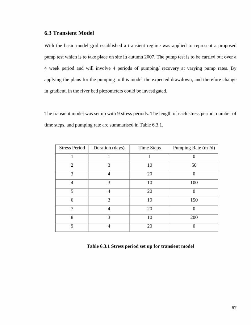
67

6.3 Transient Model

With the basic model grid established a transient regime was applied to represent a proposed

pump test which is to take place on site in autumn 2007. The pump test is to be carried out over a

4 week period and will involve 4 periods of pumping/ recovery at varying pump rates. By

applying the plans for the pumping to this model the expected drawdown, and therefore change

in gradient, in the river bed piezometers could be investigated.

The transient model was set up with 9 stress periods. The length of each stress period, number of

time steps, and pumping rate are summarised in Table 6.3.1.

Stress Period Duration (days) Time Steps Pumping Rate (m3/d)

1 1 1 0

2 3 10 50

3 4 20 0

4 3 10 100

5 4 20 0

6 3 10 150

7 4 20 0

8 3 10 200

9 4 20 0

Table 6.3.1 Stress period set up for transient model

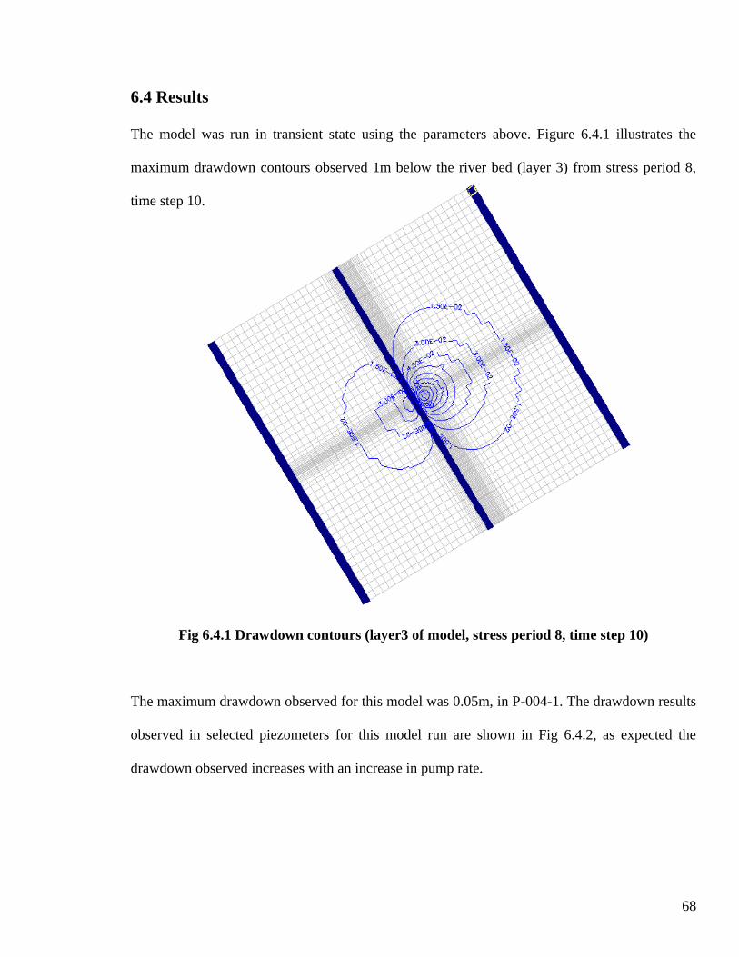
68

6.4 Results

The model was run in transient state using the parameters above. Figure 6.4.1 illustrates the

maximum drawdown contours observed 1m below the river bed (layer 3) from stress period 8,

time step 10.

Fig 6.4.1 Drawdown contours (layer3 of model, stress period 8, time step 10)

The maximum drawdown observed for this model was 0.05m, in P-004-1. The drawdown results

observed in selected piezometers for this model run are shown in Fig 6.4.2, as expected the

drawdown observed increases with an increase in pump rate.

69

0.00E+00

1.00E-02

2.00E-02

3.00E-02

4.00E-02

5.00E-02

6.00E-02

1.00E+00 6.00E+00 1.10E+01 1.50E+01 2.00E+01 2.50E+01 2.90E+01

Time (days)

Dra

wd

ow

n (

m)

.

P-022-2

P-090-1

P-004-1

P+023-2

P+070-2

Figure 6.4.2 Drawdown curves for selected piezometers from initial model run, as expected

piezometers nearest to the borehole show the highest drawdown.

To calculate the change in hydraulic gradient within the river bed sediments, the drawdown

observed in each model piezometer was subtracted from the known groundwater head level

measured in the field, to give a new groundwater head level. This was then used in the equation

described in section 4.7 to calculate a new hydraulic gradient for that piezometer. A summary of

the gradient changes are given in Table 6.4.2.

Pumping at a rate of 200m3/d will have a significant effect on the hydraulic gradients in the river

bed sediments, reducing them by between 2.6% and 48.51%.

70

Piezometer Initial

Gradient Gradient when Pump = 200m3/d

Percentage Change

P+005-1 0.1957 0.148 -24.37%

P+005-2 0.2381 0.2 -16.00%

P+005-3 0.1216 0.0845 -30.51%

P-004-2 0.0806 0.0415 -48.51%

P-004-3 0.1333 0.0955 -28.36%

P-022-2 0.0729 0.0515 -29.36%

P-022-3 0.1833 0.1605 -12.44%

P+023-2 0.0875 0.0675 -22.86%

P-050-1 0.1 0.0903 -9.70%

P+070-1 0.0213 0.0155 -27.23%

P+070-2 0.04 0.034 -15.00%

P-090-2 0.1351 0.1303 -3.55%

P-090-1 0.0566 0.05245 -7.33%

P+110-2 0.0233 0.021 -9.87%

P+110-1 0.0652 0.0635 -2.61%

Table 6.4.2 Summary of hydraulic gradient changes observed in river bed sediments when

pumping at 200m3/d

A second model was run; this time the vertical change in the river bed sediments was considered.

The river bed between 0 m and 0.5 m depth was assigned a hydraulic conductivity value of 9.5

m/d; the river bed between 0.5 m and 1m depth was assigned a hydraulic conductivity value of

2.3 m/d. These values were taken from the fieldwork data, as discussed in chapter 5. All other

hydraulic parameters remained the same.

Using these values for the river bed sediments reduces the drawdown observed in the

piezometers, to 0.048 m in P-004-1, a 4% reduction in comparison to the previous model (see

Fig 6.4.3). The most significant change is in the hydraulic gradients. Table 6.4.3 summarises the

changes in hydraulic gradient for this model run. The change in hydraulic gradient for this model

run is much less than in the initial model run, ranging between 2.07% and 38.59%.

71

0.00E+00

1.00E-02

2.00E-02

3.00E-02

4.00E-02

5.00E-02

6.00E-02

1.00E+00 6.00E+00 1.10E+01 1.50E+01 2.00E+01 2.50E+01 2.90E+01

Time (days)

Dra

wd

ow

n (

m)

P-022-2

P-090-1

P-004-1

P+023-2

P+070-2

Figure 6.4.3 Drawdown curves for selected piezometers from second model run (the two

river bed layers have been assigned different values) as expected piezometers nearest to the

borehole show the highest drawdown.

Piezometer Initial

Gradient Gradient when Pump =

200m^3/d Percentage

Change

P+005-1 0.1957 0.1575 -19.52%

P+005-2 0.2381 0.208 -12.64%

P+005-3 0.1216 0.09 -25.99%

P-004-2 0.0806 0.0495 -38.59%

P-004-3 0.1333 0.101 -24.23%

P-022-2 0.0729 0.0545 -25.24%

P-022-3 0.1833 0.164 -10.53%

P+023-2 0.0875 0.0715 -18.29%

P-050-1 0.1 0.092 -8.00%

P+070-1 0.0213 0.0165 -22.54%

P+070-2 0.04 0.035 -12.50%

P-090-2 0.1351 0.1323 -2.07%

P-090-1 0.0566 0.0531 -6.18%

P+110-2 0.0233 0.02145 -7.94%

P+110-1 0.0652 0.0636 -2.45%

Table 6.4.3 Summary of hydraulic gradient changes observed in river bed sediments when

pumping at 200m3/d during second model run

72

6.5 Use of Model As A Predictive Tool

The two initial model runs indicate that the model could be used to give an estimate of the

hydraulic gradient change that may be observed in the river bed sediments. The change in

gradient could be significant, by up to 50% in the piezometers closest to the borehole. However

as has already been shown the observed change in hydraulic gradient can vary significantly

depending on the value of hydraulic conductivity assigned to the river bed sediments in the

model.

It is probably more realistic to use the second model as a predictive indicator of gradient changes

as this takes into account some of the variability which exists in the river bed sediments.

However, as has already been discussed, there is a significant degree of heterogeneity within the

river bed sediments, and this may need to be represented to a greater degree to give a better

indication of the expected gradient changes.

This has not been done as part of the present project due to a limited amount of data and time

being available. Defining the extent of the heterogeneities within the river bed will be ‘easier’ to

do when there is actual pump test data available to calibrate the model. The extent of the

heterogeneities could be defined by comparing observed piezometer drawdown data with the

calculated drawdown in this model to assess where differences lie.

73

6.6 Sensitivity Analysis

A series of tests were carried out to assess the sensitivity of the model to different hydraulic

parameters, in particular for the hydraulic conductivity values of the layers of glacio-fluvial and

river terrace deposits, the exact values of which are uncertain.

The hydraulic conductivity for each zone was analyzed by changing one parameter at a time and

assessing the effect the change had on the drawdown in each piezometer. Some of the zones for

hydraulic conductivity were highly sensitive relative to other zones.

The analysis found that the model was very sensitive to changes in conductivity in layers 1 to 3,

in particular the river bed sediments. Decreasing the hydraulic conductivity by a factor of two

was found to increase the drawdown by a factor of two; the layer 2 river bed sediments in

particular had a big effect on the drawdown.

The model was slightly sensitive to changes in the hydraulic conductivity of layers 4 to 21

(glacio-fluvial and river terrace deposits), with the upper layers (4 to17) having the biggest

effect. This indicates the need to have a good representative hydraulic conductivity value for the

superficial deposits, and is something which may need investigating further.

The model was generally insensitive to change in the specific yield, with only layer 1 showing

any sensitivity

74

6.7 Conclusions

The modelling results have indicated that pumping at a discharge rate of 200m3/d from the

borehole at the study site will significantly influence the hydraulic gradients observed within the

river bed sediments. A gradient reduction of up to 50% can be expected in the piezometers

closest to the borehole. At the present time the second model run described above is thought to

best represent the system, as it takes into account the vertical change in hydraulic conductivity of

the river bed sediments.

The sensitivity analysis indicates that constraining the hydraulic conductivity values of the river

bed sediments and upper layers of the superficial drift deposits will have the most effect on the

on the drawdowns observed in the model.

More data is needed to calibrate the model, which will be gained when the pump tests are carried

out. This will help make the model more accurate, and in particular help constrain the

heterogeneities within the river bed sediments and drift deposits.

75

Chapter 7. Conclusions

7.1 Summary

The aims of this project were to investigate the hydraulic properties of the aquifer system and

examine the effects of a hydraulic test on the hydraulic gradients observed below the river bed.

Relevant conclusions from individual areas of investigation have already been presented in

chapters 5 and 6. This section concludes generally on the aims and objectives of the study.

A comprehensive network of piezometers has been installed at various depths and locations

within the river bed which have given a good set of data results for this project and can continue

to be used as part of the future research on site. Falling head tests and groundwater head

measurements carried out on the piezometers indicated the varied nature of the river bed

sediments hydraulic properties. The hydraulic conductivity (2 m/d) calculated from the pump test

on the Kidderminster Sandstone, correlated well with previous pump test data, indicating that a

single-well pump test can provide valuable data.

A basic groundwater flow model of the study area was completed. Simulations of hydraulic tests

indicated that, significant changes to the natural hydraulic gradients below the river bed could be

achieved (up to 50%). It is recommended that a pump rate of 200m3/d could be used for future

tests as this will cause a significant degree of mixing within the hyporheic zone. More data is

required to calibrate the model and assess the importance of heterogeneities within the river bed

sediments and superficial drift deposits.

76

7.2 Future Work

A number of recommendations are made for future work on the site, in particular to help

improve upon the understanding of the hydraulic properties developed in this project:

A repeat of all falling head tests on the piezometers is required in order to assess if there

is any variability in hydraulic conductivity due to river bed sediments having more time

to settle around the piezometers following the disturbance caused during their

installation.

Install new, longer piezometers (or find a better method for extending the tubes of the

current piezometers) at P+070-1, P+070-2 and P+110-2, in order to conduct successful

falling head tests at these locations.

Install a new piezometer next to P-022-1 to assess if the difficulty in conducting a

successful falling head test was due to a very low permeability horizon or due to damage

to the piezometers open section.

Carry out the pump tests detailed in chapter 6, recording data from all piezometers and

the pumping borehole, to give a detailed data set which can be used for more calculations

of the systems hydraulic properties.

Use pump test data to fully calibrate the current groundwater flow model and assess the

extent and importance of heterogeneities within the aquifer and river bed sediments.

Use the newly calibrated model to investigate the changes in hydraulic gradients below

the river bed as part of the plan for any future experiments carried out on the site.

77

References

Biksey, T.M. & Gross, E.D., 2001. The hyporheic zone: Linking groundwater and surface water

– Understanding the paradigm. Remediation Journal 12(1), 55-62.

Boulton, A.J., Findlay, S., Marmonier, P., Stanley, E.H. & Valett, H.M., 1998. The functional

significance of the hyporheic zone in streams and rivers. Annual Review of Ecology and

Systematics 29, 59-81.

Calver, A., 2001. Riverbed permeabilities: Information from pooled data. Ground Water 39(4),

546-553.

Conran, D.J., 2006. Assessment of groundwater-surface water mixing zone transients:

Birmingham – River Tame study. Unpublished MSc thesis, School of Earth Sciences, University

of Birmingham.

Driscoll, F.G., 1995. Groundwater and wells, 2nd

Ed. Published by USF Filter/Johnson Screens.

Ellis, P.A., Mackay, R. & Rivett, M.O., 2007. Quantifying urban river-aquifer fluid exchange

processes: A multi-scale problem. Journal of Contaminant Hydrology 91, 58-80.

78

Ellis, P.A., 2002. The impact of urban groundwater upon surface water quality: Birmingham –

River Tame study, UK. Unpublished PhD thesis, School of Earth Sciences, University of

Birmingham.

Environment Agency, 2002. The Water Framework Directive: Guiding principles on the

technical requirements. Environment Agency, Bristol.

Greswell, R.B., 1992. The modelling of groundwater rise in the Birmingham area. Unpublished

MSc thesis, School of Earth Sciences, University of Birmingham.

Griffiths, J., Binley, A., Crook, N. Nutter, J., Young, A. & Fletcher, S., 2006. Streamflow

generation on the Pang and Lambourn catchments, Berkshire, UK. Journal of Hydrology 330,

71-83.

Halford, K.J., Weight, W.D. & Schreiber, R.P., 2006. Interpretation of transmissivity estimates

from single-well pumping aquifer tests. Ground Water 44(3), 467-471.

Hancock, P.J., 2002. Human impacts on the stream-groundwater exchange zone. Environmental

Management 29(6), 763-781.

Harvey, J.W. & Wagner, B.J., 2000. Quantifying hydrologic interactions between streams and

their subsurface hyporheic zones. In: Streams & Ground Waters. Eds. Jones, J.B. & Mulholland,

P.J. Published by Academic Press, 3-44.

79

Hiscock, K., 2005. Hydrogeology principles and practice. Published by Blackwell publishing.

Lydon, C., 2006. Design for the hyporheic zone dipole setup. Unpublished MSc thesis, School of

Earth Sciences, University of Birmingham.

Powell, J.H., Glover, B.W. & Waters, C.N., 2000. Geology of the Birmingham area.

Memoir of the British Geological Survey Sheet 168 (England & Wales).

Rivett, M.O., Greswell, R.B., Mackay, R., Lydon, C., Conran, D.J. & Ellis, P.A., 2006. Natural

attenuation potential of the urban hyporheic zone: Foundational studies to the River Tame

(Birmingham, UK) dipole field experiments. SWITCH Report.

Rushton, K.R., 2003. Groundwater Hydrology: Conceptual and Computational Models.

Published by Wiley.

Shaw, E.M., 1991. Hydrology in practice, 2nd

Ed. Published by Chapman & Hall, London.

Shepherd, K.A., Ellis, P.A. & Rivett, M.O. 2006. Integrated understanding of urban land,

groundwater, baseflow and surface-water quality – The City of Birmingham, UK. Science of the

Total Environment 360, 180-195.

Smith, J.W.N., 2005. Groundwater – surface water interactions in the hyporheic zone.

80

Environment Agency Science Report SC030155/SR1.

SMURF, 2005. Sustainable Management of Urban Rivers and Floodplains (SMURF). SMURF

Project Summary Report.

Sophocleous, M., 2002. Interactions between groundwater and surface water: the state of

science. Hydrogeology Journal 10, 52-67.

Triska, F.J., Kennedy, V.C., Avanzino, R.J., Zellweger, G.W., & Bencala, K.E., 1989. Retention

and transport of nutrients in a third order stream in Northwestern California: Hyporheic

Processes. Ecology 70(6), 1893-1905.

Wheater, H.S., Peach, D. & Binley, A., 2007. Characterising groundwater dominated lowland

catchments: the UK Lowland Catchment Research Programme (LOCAR). Hydrology and Earth

Systems Science 11(1), 108-124.

Winter, T.C., 2000. Interaction of ground water and surface water. Proceedings of the Ground-

Water/Surface-Water Interactions Workshop, 15-20. Environmental Protection Agency (U.S.)

Report EPA/542/R-00/007.

Winter, T.C., Harvey, J.W., Franke, O.L. & Alley, W.M., 1998. Ground water and surface water

a single resource. United States Geological Survey, Circular 1139.

81

Woessner, W.W., 2000. Stream and fluvial plain ground Water interactions: Rescaling

hydrogeological thought. Ground Water 38(3), 423-429.

Yamada, H., Nakamura, F., Watanabe, Y., Murakami, M. & Nogami, T., 2005. Measuring

hydraulic permeability in a streambed using the packer test. Hydrological Processes 19, 2507-

2524.