Hyperparameter Search Space Pruning � A New

Component for Sequential Model-Based

Hyperparameter Optimization

Martin Wistuba, Nicolas Schilling, and Lars Schmidt-Thieme

Information Systems and Machine Learning LabUniversitätsplatz 1, 31141 Hildesheim, Germany

{wistuba,schilling,schmidt-thieme}@ismll.uni-hildesheim.de

Abstract. The optimization of hyperparameters is often done manu-ally or exhaustively but recent work has shown that automatic methodscan optimize hyperparameters faster and even achieve better �nal per-formance. Sequential model-based optimization (SMBO) is the currentstate of the art framework for automatic hyperparameter optimization.Currently, it consists of three components: a surrogate model, an acquisi-tion function and an initialization technique. We propose to add a fourthcomponent, a way of pruning the hyperparameter search space which isa common way of accelerating the search in many domains but yet hasnot been applied to hyperparameter optimization. We propose to discardregions of the search space that are unlikely to contain better hyperpa-rameter con�gurations by transferring knowledge from past experimentson other data sets as well as taking into account the evaluations alreadydone on the current data set.Pruning as a new component for SMBO is an orthogonal contributionbut nevertheless we compare it to surrogate models that learn acrossdata sets and extensively investigate the impact of pruning with andwithout initialization for various state of the art surrogate models. Theexperiments are conducted on two newly created meta-data sets whichwe make publicly available. One of these meta-data sets is created on 59data sets using 19 di�erent classi�ers resulting in a total of about 1.3million experiments. This is by more than four times larger than all theresults collaboratively collected by OpenML.

1 Introduction

Most machine learning algorithms depend on hyperparameters that need to betuned. In contrast to model parameters, hyperparameters are not estimated dur-ing the learning process but have to be set before. Since the hyperparametertuning often decides whether the performance of an algorithm is state of the artor just moderate, the task of hyperparameter optimization is as important asdeveloping new models [2,7,20,22,25]. Typical hyperparameters are for examplethe trade-o� parameter C of a support vector machine or the regularization con-stant of a Tikhonov-regularized model. Taking a step further, the chosen model

as well as preprocessing steps can be considered as hyperparameters [25]. Then,hyperparameter optimization not only involves model selection but also modelclass selection, choice of learning algorithms and preprocessing.

The conventional way of hyperparameter optimization is a combination ofmanual search with a grid search. This is an exhaustive search in the hyperpa-rameter space which involves multiple training of the model. For high-complexhyperparameter spaces or large data sets this becomes infeasible. Therefore,methods to accelerate the process of hyperparameter optimization are currentlyan interesting topic for researchers [3,22,25]. Sequential model-based optimiza-tion (SMBO) [15] is a black-box optimization process and has proven to be ef-fective in accelerating the hyperparameter optimization process. SMBO is basedon a surrogate model that approximates the response function of a data set forgiven hyperparameters such that sequentially possibly interesting hyperparam-eter con�gurations can be evaluated.

Recent work tries to transfer knowledge about the hyperparameter spacefrom past experiments to a new data set [1,24,29]. They motivate this idea byassuming that regions of the hyperparameter space that perform well for fewdata sets likely contain promising hyperparameter con�gurations for new datasets.

1.1 Our Contributions

The SMBO framework currently has at most three components. First, the sur-rogate model that predicts the performance for each possible hyperparametercon�guration. Secondly, the acquisition function which uses the surrogate modelto propose the next hyperparameter con�guration to evaluate. These are thetwo mandatory components. The third optional component is some initializa-tion technique which usually starts which a hyperparameter con�guration thathas proven to be good on many data sets [9,11]. We propose to add a fourthcomponent which is orthogonal to all the others. Our idea is to reduce the hy-perparameter search space by using knowledge from past experiments to discardregions that are very likely not interesting. This avoids that the acquisitionfunction chooses hyperparameter con�gurations in these regions because of highuncertainty and therefore avoids unnecessary function evaluations.

Additionally, we created two meta-data sets and make them publicly avail-able. One is a meta-data set created by running a kernel support vector machineon 50 di�erent data sets with 288 di�erent hyperparameter con�gurations re-sulting into 14,000 meta-instances. The second is a large scale meta-data setcreated by using 19 di�erent classi�ers provided by Weka [13] on 59 data sets.In total 1,290,389 meta-instances were created such that the number of runs isby more than 4 times larger than the number of runs collaboratively collectedby OpenML [26].

2 Related Work

Pruning is a well known technique to accelerate the search in several domains.Thus, for example, various pruning techniques are applied to the minimax algo-rithm such as the killer heuristic or null move pruning [8]. Branch-and-Bound[18] is a pruning technique that is applied in the domain of operations researchfor discrete and combinatorial optimization problems and is very common forNP-hard optimization problems [17]. Nevertheless, we are not aware of any pub-lished work that is trying to prune the search space in the SMBO framework forhyperparameter optimization.

Since pruning as proposed by us is some way of transferring knowledge frompast experiments to a new experiment, other techniques that try exactly the sameare the closest related work but as we will see, orthogonal to our contribution.One common and easy way to use experience in the hyperparameter optimizationdomain is to de�ne an initialization, a sequence of hyperparameter con�gurationsthat are chosen �rst. These are usually those hyperparameter con�gurations thatperformed best on average across data sets [9,11]. The second and last methodto do so is by using the surrogate model. Instead of learning the surrogate modelonly on the new data set, the surrogate model is learned across all data sets[1,24,29]. We want to highlight that all these three possibilities are not mutuallyexclusive and can be combined and thus these ideas are orthogonal to each other.

Leite et al. [19] propose a similar distance function between data sets as weuse. But they propose a hyperparameter selection strategy that is limited to thehyperparameter con�gurations that have been seen on the meta-training data.

Furthermore, there also exist strategies to optimize hyperparameters that arebased on optimization techniques from arti�cial intelligence such as tabu search[4], particle swarm optimization [12] and evolutionary algorithms [10] as well asgradient-based optimization techniques [6] designed for SVMs.

3 Background

3.1 The Formal Setup

A machine learning algorithm Aλ is a mapping Aλ : D → M where D is theset of all data sets, M is the space of all models and λ ∈ Λ is the chosenhyperparameter con�guration with Λ = Λ1 × . . . × Λp being the p-dimensionalhyperparameter space. The learning algorithm estimates a model Mλ ∈M thatminimizes a regularized loss function L (e.g. misclassi�cation rate):

Aλ(D(train)

):= arg min

Mλ∈ML(Mλ, D

(train))+R (Mλ) . (1)

Then, the task of hyperparameter optimization is �nding the optimal hyperpa-rameter con�guration λ∗ using a validation set i.e.

λ∗ := argminλ∈ΛL(Aλ(D(train)

), D(valid)

):= argmin

λ∈ΛfD (λ) . (2)

3.2 Sequential Model-based Optimization

Exhaustive hyperparameter search methods such as grid search are becomingmore and more expensive. Data sets are growing, models are getting more com-plex and have high-dimensional hyperparameter spaces. Sequential model-basedoptimization (SMBO) [15] is a black-box optimization framework that replacesthe time-consuming function f to evaluate with a cheap-to-evaluate surrogatefunction Ψ that approximates f . With the help of an acquisition function suchas expected improvement [15] it sequentially chooses new points such that a bal-ance between exploitation and exploration is found and f is optimized. In ourscenario evaluating f is equivalent to learning a model on some training datafor a given hyperparameter con�guration and estimating the performance of thismodel on a hold-out data set.

Algorithm 1 outlines the SMBO framework. It starts with an observationhistory H that equals the empty set in cases where no knowledge from pastexperiments is used [2,14,22] or is non-empty in cases where past experimentsare used [1,24,29]. First, the optimization process can be initialized. Then, thesurrogate model Ψ is �tted to H where Ψ can be any regression model. Since theacquisition function usually needs to assess prediction uncertainty of the surro-gate, common choices are Gaussian processes [1,22,24,29] or ensembles such asrandom forests [14]. The acquisition function chooses the next candidate to eval-uate. A common choice for the acquisition function is expected improvement [15]but further acquisition functions exist such as probability of improvement [15],the conditional entropy of the minimizer [27] or a criterion based on multi-armedbandits [23]. The evaluated candidate is �nally added to the set of observations.After T -many SMBO iterations, the best currently found hyperparameter con-�guration is returned.

Line 6 is our proposed addition to the SMBO framework. Selecting the iden-tity function as prune results in the typical SMBO framework. In the next sectionwe propose a more suitable pruning function.

Algorithm 1 Sequential Model-based Optimization

Input: Hyperparameter space Λ, observation historyH, number of iterations T , acqui-sition function a, surrogate model Ψ , initial hyperparameter con�gurations Λ(init).

Output: Best hyperparameter con�guration found.1: for λ ∈ Λ(init) do

2: Evaluate f (λ)3: H ← H∪ {(λ, f (λ))}4: for t =

∣∣∣Λ(init)∣∣∣+ 1 to T do

5: Fit Ψ to H6: Λ(pruned) ← prune (Λ)7: λ← argmaxλ∈Λ(pruned) a (λ, Ψ)8: Evaluate f (λ)9: H ← H∪ {(λ, f (λ))}10: return argmax(λ,f(λ))∈H f (λ)

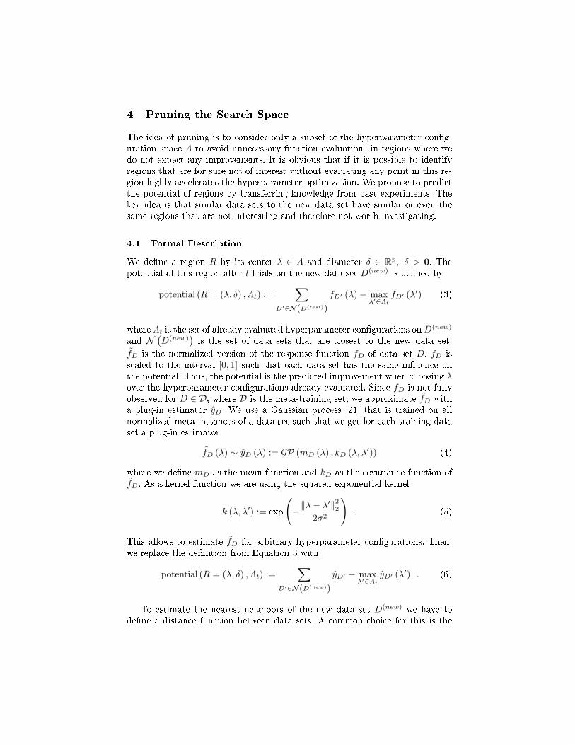
4 Pruning the Search Space

The idea of pruning is to consider only a subset of the hyperparameter con�g-uration space Λ to avoid unnecessary function evaluations in regions where wedo not expect any improvements. It is obvious that if it is possible to identifyregions that are for sure not of interest without evaluating any point in this re-gion highly accelerates the hyperparameter optimization. We propose to predictthe potential of regions by transferring knowledge from past experiments. Thekey idea is that similar data sets to the new data set have similar or even thesame regions that are not interesting and therefore not worth investigating.

4.1 Formal Description

We de�ne a region R by its center λ ∈ Λ and diameter δ ∈ Rp, δ > 0. Thepotential of this region after t trials on the new data set D(new) is de�ned by

potential (R = (λ, δ) , Λt) :=∑

D′∈N(D(test))

fD′ (λ)− maxλ′∈Λt

fD′ (λ′) (3)

where Λt is the set of already evaluated hyperparameter con�gurations onD(new)

and N(D(new)

)is the set of data sets that are closest to the new data set.

fD is the normalized version of the response function fD of data set D. fD isscaled to the interval [0, 1] such that each data set has the same in�uence onthe potential. Thus, the potential is the predicted improvement when choosing λover the hyperparameter con�gurations already evaluated. Since fD is not fullyobserved for D ∈ D, where D is the meta-training set, we approximate fD witha plug-in estimator yD. We use a Gaussian process [21] that is trained on allnormalized meta-instances of a data set such that we get for each training dataset a plug-in estimator

fD (λ) ∼ yD (λ) := GP (mD (λ) , kD (λ, λ′)) (4)

where we de�ne mD as the mean function and kD as the covariance function offD. As a kernel function we are using the squared exponential kernel

k (λ, λ′) := exp

(−‖λ− λ′‖22

2σ2

). (5)

This allows to estimate fD for arbitrary hyperparameter con�gurations. Then,we replace the de�nition from Equation 3 with

potential (R = (λ, δ) , Λt) :=∑

D′∈N(D(new))

yD′ − maxλ′∈Λt

yD′ (λ′) . (6)

To estimate the nearest neighbors of the new data set D(new) we have tode�ne a distance function between data sets. A common choice for this is the

Euclidean distance with respect to the meta-features [1,29]. Since we experiencedbetter results with a distance function based on rank correlation metrics such asthe Kendall tau rank correlation coe�cient [16], we are using following distancefunction

KTRC(D1, D2, Λt) :=∑λ1,λ2∈Λt

I(yD1(λ1)>yD1

(λ2)⊕yD2(λ1)>yD2

(λ2))(|Λt|−1)|Λt| (7)

where ⊕ is the symbol for an exclusive or.

Algorithm 2 Prune

Input: Hyperparameter space Λ, observation history H, region radius δ, fraction ofthe pruned space ν.

Output: Pruned hyperparameter space Λpruned ⊆ Λ.1: Estimate the most similar data sets of the new data set N (Dnew) using Equation

7.2: Estimate the set Λ′ containing the ν |G| hyperparameter con�gurations λ′ ∈ G ⊂ Λ

with little potential using Equation 6.3: Λ(pruned) := {λ ∈ Λ | dist (λ, λ′) > δ, λ′ ∈ Λ′}.4: return Λ(pruned) ∪ {λ ∈ Λ | dist (λ, λ′) ≤ δ, λ′ ∈ Λt}

Algorithm 2 summarizes the pruning function. Line 1 estimates the k mostsimilar data sets which we know from past experiments using the KTRC dis-tance function de�ned in Equation 7. In Line 2 the potential of hyperparametercon�gurations are estimated using the plug-in estimators (Equation 6) on a �negrid G ⊂ Λ. The ν |G| hyperparameter con�gurations with little potential de�neregions where no improvement is predicted. Hence, the pruned hyperparameterspace is de�ned as the set of hyperparameter con�gurations that are not withinan δ-region of these low-potential hyperparameter con�gurations (Line 3). Addi-tionally, the hyperparameter con�gurations that are within a δ-region of alreadyevaluated hyperparameter con�gurations are added (Line 4). The intuition hereis that since we have already observed an evaluation in this region, the acquisi-tion function will not choose a hyperparameter combination close to these pointsfor exploration but only for exploitation. Hence, no evaluations will be done bythe standard SMBO framework without a very likely improvement. For the dis-tance function between hyperparameter con�gurations we need to consider onethat does not take discrete variables into account. Obviously, the loss does notchange smoothly when changing a categorical variable that e.g. indicates whichalgorithm was chosen. Therefore, we de�ne the distance function in Algorithm2 as

dist (λ, λ′) :=

{∞ if λ and λ′ di�er in a categorical variable

‖λ− λ′‖ otherwise. (8)

5 Experimental Evaluation

First, we will introduce the reader to the state of the art tuning strategies whichare used to evaluate pruning. Then, the evaluation metrics are de�ned and themeta-data sets are introduced. Finally, the results are presented.

5.1 Tuning Strategies

We want to give a short introduction to all the tuning strategies we will con-sider in our experiments. We are considering both strategies that are using noknowledge from previous experiments and those that do.

Random Search This is the only strategy that is not using any surrogate model.Hyperparameter con�gurations are sampled uniformly at random. This is a com-mon strategy in cases where a grid search is not possible. Bergstra and Bengio[3] have shown that this is very e�ective for hyperparameters with low e�ectivedimensionality.

Independent Gaussian Process (I-GP) This tuning strategy uses a Gaussianprocess [22] with squared-exponential kernel as a surrogate model. It only usesknowledge from the current data set and is not using any knowledge from pre-vious experiments.

Independent Random Forest (I-RF) Next to Gaussian processes, random forestsare the most widely used surrogate models [14] and hence we are using them inour experiments. Like the independent Gaussian process, the I-RF does not useany knowledge from previous experiments.

Sequential Model-based Algorithm Con�guration++ (SMAC++) SMAC [14] isa tuning strategy that is based on a random forest as a surrogate model withoutbackground knowledge of previous experiments. SMAC++ is our extension toSMAC. SMAC++ is using the typical SMBO framework but the random forestis also trained on the meta-training data.

Surrogate Collaborative Tuning (SCoT) SCoT [1] uses a Gaussian process withsquared-exponential kernel with automatic relevance determination and is trainedon hyperparameter observations of previous experiments evaluated on other datasets and the few knowledge achieved on the new data set. An SVMRank is learnedon the data set and its predictions are used instead of the hyperparameter per-formances. Bardenet et al. [1] argue that this overcomes the problem of havingdata sets with di�erent scales of hyperparameter performances. In the originalwork it was proposed to use an RBF kernel for SVMRank. For reasons of com-putational complexity we follow the lead of Yogatama and Mann [29] and use alinear kernel instead.

Gaussian Process with MKL (MKL-GP) Similarly to Bardenet et al. [1], Yo-gatama and Mann [29] propose to use a Gaussian process as a surrogate modelfor the SMBO framework. Instead of using SVMRank to deal with the di�erentscales, they are adapting the mean of the Gaussian process, accordingly. Addi-tionally, they are using a speci�c kernel, a linear combination of an SE-ARDkernel with a kernel modelling the distance between data sets.

Optimal This is an arti�cial tuning strategy that always evaluates the besthyperparameter con�guration and is added to plots for orientation purposes.

Kernel parameters are learned by maximizing the marginal likelihood on themeta-training set [21]. Hyperparameters of the tuning strategies are optimizedin a leave-one-out cross-validation on the meta-training set.

The results reported are the average of at least ten repetitions. For the strate-gies with random initialization (Random, I-GP, I-RF), the mean of 1000 repeti-tions is reported.

5.2 Evaluation Metrics

In our experiments we are using three di�erent evaluation metrics which we willexplain here in detail.

Average Rank The average rank among di�erent hyperparameter tuning strate-gies or for short simply average rank is a relative metric between di�erent tuningstrategies. The tuning strategies are ranked by the best hyperparameter con�g-uration that they have found so far, ties are solved by granting them the averagerank. If we have for example four di�erent tuning strategies that have foundhyperparameter con�gurations that achieve an accuracy of 0.78, 0.77, 0.77 and0.76, respectively, then the ranking is 1, 2.5, 2.5 and 4.

Normalized Average Loss The disadvantage of the average rank is that it givesno information about by which margin the found hyperparameters of one tuningstrategy are better than another and it will vary when strategies are added or areremoved. One metric that overcomes this disadvantage is the normalized averageloss. In our experiments we will consider only classi�cation problems such thatfD (λ) is the accuracy on data set D using hyperparameter con�guration λ.Since the scale of fD varies for di�erent D we normalize fD between 0 and 1such that every data set has the same impact on the evaluation metric. Thus,the normalized average loss at iteration t is de�ned as

NAL (D, Λt) :=1

|D|∑D∈D

1− maxλ∈Λt fD (λ)−minλ∈Λ fD (λ)

maxλ∈Λ fD (λ)−minλ∈Λ fD(λ). (9)

Average Hyperparameter Rank The average hyperparameter rank is another wayto overcome the disadvantages of the average rank. Compared to the averagerank it is not ranking the tuning strategies but ranking the hyperparametercon�gurations. Let rD (λ) be the rank of the hyperparameter con�guration λ ondata set D, then the average hyperparameter rank is de�ned as

AHR(D, Λt) :=1

|D|∑D∈D

minλ∈Λt

rD (λ)− 1 . (10)

5.3 Meta-Data Sets

The SVM meta-data set was created by using 50 classi�cation data sets chosenat random. All instances were merged in cases where splits were already given,shu�ed and split into 80% train and 20% test. We then used a support vectormachine (SVM) [5] to create the meta-instances. We trained the SVM using threedi�erent kernels (linear, polynomial and Gaussian) and estimated the labelsof the meta-instances by evaluating the trained model on the test split. Thehyperparameter space dimension is six, three dimensions for binary features thatindicate which kernel was chosen, one for the trade-o� parameter C, one for thedegree of the polynomial kernel d and the width γ of the Gaussian kernel. If thehyperparameter is not involved, e.g. the degree if we are using the linear kernel,it was set to 0. The test accuracy was precomputed on a grid C ∈

{2−5, . . . , 26

},

d ∈ {2, . . . , 10}, γ ∈{10−4, 10−3, 10−2, 0.05, 0.1, 0.5, 1, 2, 5, 10, 20, 50, 102, 103

}resulting into 288 meta-instances per data set. Since meta-features are a vitalpart for many surrogate models and mandatory for SCoT and MKL-GP, weadded the meta-features that were used by [1,29] to our meta-data. First , weextracted the number of training instances n, the number of classes c and thenumber of predictors m. The �nal meta-features are c, log (m) and log (n/m)scaled to [0.1].

The Weka meta-data set was created using 59 classi�cation data sets whichwere preprocessed like the classi�cation data sets used for the SVM meta-dataset. We used 19 di�erent Weka classi�ers [13] and produced 21,871 hyperparam-eter con�gurations per data set. The dimension of the hyperparameter space is102 including the indicator variables for the classi�er. Thus, this meta-data setfocuses stronger on the model class selection. Overall, this meta-data set contains1,290,389 instances. In comparison, OpenML [26] has collaboratively collected344,472 runs.1

The meta-data sets are available on our supplementary website together witha visualization of the meta-data as well as more details about how the meta-datasets were created and a detailed list which data sets were used [28].

5.4 Hyperparameter Optimization for SVMs

To show that the proposed plug-in estimators work (Equation 4), we did not useall 288 hyperparameter con�gurations for training but only 50 per data set. The

1 Status 2015/03/27 by http://openml.org

evaluation is nevertheless done on all 288 of the new data set. We choose G tocontain these 288 con�gurations and �xed |N (Dnew)| = 2, ν = 1− |G|−1 and δsuch that the two closest neighbored hyperparameter con�gurations of the testregion are within δ-distance.

We want to conduct two di�erent experiments. First, we want to compare asurrogate model with pruning to current state of the art tuning strategies. Weonce again want to stress that pruning in the SMBO framework is an orthogonalcontribution such that these results are actually of minor interest. Second, wewant to compare di�erent surrogate models with and without pruning or ini-tialization. Pruning is a useful contribution as long as it does not worsen theoptimization speed in general and accelerates it in some cases.

Figure 1 shows the results of the comparison of pruning to the current stateof the art method. As a surrogate model we decided to choose the Gaussianprocess that is not learned across data sets since it is the most common andsimple surrogate model. Surprisingly, the pruning alone with the Gaussian pro-cess is able to outperform all the competitor strategies with respect to all threeevaluation metrics.

I−GP (pruned)

Optimal

2

4

6

0 20 40 60Number of Trials

Ave

rage

Ran

k

10−2

10−1.5

10−1

10−0.5

0 20 40 60Number of Trials

Nor

mal

ized

Ave

rage

Los

s

10−0.5

100

100.5

101

101.5

102

0 20 40 60Number of Trials

Ave

rage

Hyp

erpa

ram

eter

Ran

k

Random I−GP I−RF SMAC++ SCoT MKL−GP I−GP (pruned) Optimal

Fig. 1. Pruning is an orthogonal contribution to the SMBO framework. Nevertheless,we compare a pruned independent Gaussian process to many current state of the arttuning strategies without pruning.

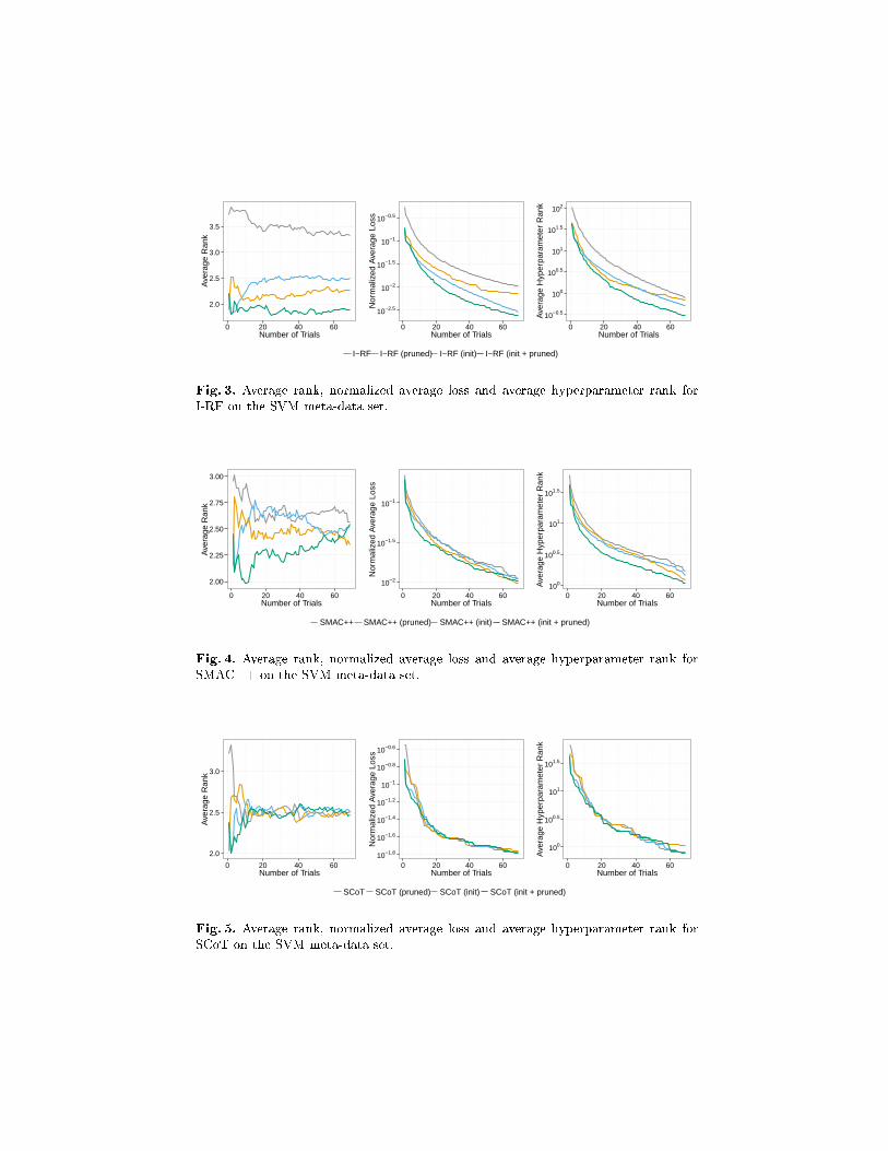
Figures 2 to 6 show the results of di�erent surrogate models. We distinguishfour di�erent cases: i) only the surrogate model, ii) the surrogate model withpruning, iii) the surrogate model with three steps of initialization and iv) thesurrogate model with three steps of initialization and pruning. Figures 2 and 3show the results for the surrogate models that do not learn across data sets andthe remaining three Figures show the results for the surrogate models that learnacross data sets. Our expectation before the experiments were that the lift ishigher i) for the experiments without initialization and ii) for the experimentswith the surrogate models that do not learn across data sets. The reason for thisis simple. An initialization is a �xed policy that proposes hyperparameter con�g-urations that has been good on average while pruning discards regions that were

not useful. Thus, pruning will also have an e�ect of initialization. The di�er-ence between initialization and pruning is that initialization proposes a speci�chyperparameter while pruning reduces the full hyperparameter space to a setof good hyperparameter con�gurations and pruning is applied at each iterationand not just for the initial iterations. Additionally, pruning is a way to trans-fer knowledge between data sets such that those strategies that do not use thisknowledge at all bene�t more and are prevented from conducting unnecessaryexploration queries.

This is exactly what the results of the experiments show. The SMBO ex-periments with pruning have comparable good starting points like those withinitialization. If we compare the results of the independent Gaussian processand random forest for the setting with only initialization with the one with onlypruning, we clearly see the unnecessary exploration queries after a good start.The setting with both initialization and pruning does not su�er from this prob-lem and thus is clearly the best strategy. This e�ect is weaker for the surrogatemodels that are learned across data sets in Figures 4 and 6. Only for SCoT(Figure 5) pruning does not accelerate the hyperparameter optimization on thismeta-data set but it also does not worsen it. Table 1 shows the results for allevaluation metrics and surrogate models.

The reader may notice two important things. First, the results in the plotwill always converge to the same value across di�erent tuning strategies if youallow only enough trials. Second, even a very small improvement of the per-formance just by choosing a better hyperparameter con�gurations is already asuccess especially since this optimization is usually limited in time. This littleimprovement may result in signi�cantly better results for a new model comparedto the competitors or decides whether a research challenge will be won or not.

2.0

2.5

3.0

3.5

4.0

0 20 40 60Number of Trials

Ave

rage

Ran

k

10−3

10−2.5

10−2

10−1.5

10−1

10−0.5

0 20 40 60Number of Trials

Nor

mal

ized

Ave

rage

Los

s

10−0.5

100

100.5

101

101.5

102

0 20 40 60Number of Trials

Ave

rage

Hyp

erpa

ram

eter

Ran

k

I−GP I−GP (pruned) I−GP (init) I−GP (init + pruned)

Fig. 2. Average rank, normalized average loss and average hyperparameter rank forI-GP on the SVM meta-data set.

2.0

2.5

3.0

3.5

0 20 40 60Number of Trials

Ave

rage

Ran

k

10−2.5

10−2

10−1.5

10−1

10−0.5

0 20 40 60Number of Trials

Nor

mal

ized

Ave

rage

Los

s

10−0.5

100

100.5

101

101.5

102

0 20 40 60Number of Trials

Ave

rage

Hyp

erpa

ram

eter

Ran

k

I−RF I−RF (pruned) I−RF (init) I−RF (init + pruned)

Fig. 3. Average rank, normalized average loss and average hyperparameter rank forI-RF on the SVM meta-data set.

2.00

2.25

2.50

2.75

3.00

0 20 40 60Number of Trials

Ave

rage

Ran

k

10−2

10−1.5

10−1

0 20 40 60Number of Trials

Nor

mal

ized

Ave

rage

Los

s

100

100.5

101

101.5

0 20 40 60Number of Trials

Ave

rage

Hyp

erpa

ram

eter

Ran

k

SMAC++ SMAC++ (pruned) SMAC++ (init) SMAC++ (init + pruned)

Fig. 4. Average rank, normalized average loss and average hyperparameter rank forSMAC++ on the SVM meta-data set.

2.0

2.5

3.0

0 20 40 60Number of Trials

Ave

rage

Ran

k

10−1.8

10−1.6

10−1.4

10−1.2

10−1

10−0.8

10−0.6

0 20 40 60Number of Trials

Nor

mal

ized

Ave

rage

Los

s

100

100.5

101

101.5

0 20 40 60Number of Trials

Ave

rage

Hyp

erpa

ram

eter

Ran

k

SCoT SCoT (pruned) SCoT (init) SCoT (init + pruned)

Fig. 5. Average rank, normalized average loss and average hyperparameter rank forSCoT on the SVM meta-data set.

2.25

2.50

2.75

3.00

3.25

0 20 40 60Number of Trials

Ave

rage

Ran

k

10−3

10−2.5

10−2

10−1.5

10−1

10−0.5

0 20 40 60Number of Trials

Nor

mal

ized

Ave

rage

Los

s

10−1

10−0.5

100

100.5

101

101.5

102

0 20 40 60Number of Trials

Ave

rage

Hyp

erpa

ram

eter

Ran

k

MKL−GP MKL−GP (pruned) MKL−GP (init) MKL−GP (init + pruned)

Fig. 6. Average rank, normalized average loss and average hyperparameter rank forMKL-GP on the SVM meta-data set.

Table 1. Average rank, normalized average loss and average hyperparameter rank after30 trials on the SVM meta-data set. Best results are bold.

I-GP no pruning/init pruned init init + pruned

Average Rank@30 3.12 2.35 2.72 1.81

NAL@30 0.0224 0.0131 0.0291 0.0055

AHR@30 3.48 2.60 3.98 1.97

I-RF no pruning/init pruned init init + pruned

Average Rank@30 3.51 2.11 2.51 1.87

NAL@30 0.0281 0.0149 0.0116 0.0070

AHR@30 4.75 2.64 2.98 2.14

SMAC++ no pruning/init pruned init init + pruned

Average Rank@30 2.72 2.45 2.65 2.18

NAL@30 0.0251 0.0228 0.0256 0.0210

AHR@30 5.42 4.92 4.52 3.53

SCoT no pruning/init pruned init init + pruned

Average Rank@30 2.55 2.55 2.47 2.43

NAL@30 0.0244 0.0244 0.0237 0.0237

AHR@30 3.44 3.44 3.02 2.90

MKL-GP no pruning/init pruned init init + pruned

Average Rank@30 2.68 2.52 2.49 2.31

NAL@30 0.0349 0.0232 0.0120 0.0099

AHR@30 6.30 3.48 3.00 2.40

5.5 Hyperparameter Optimization for Weka

In the last chapter, we have seen little improvement in cases where an initial-ization is combined with surrogate models that are learning across data sets.We expect pruning to be useful in two scenarios: if i) the dimensionality of thehyperparameter space is very high and ii) the meta-data set is too large suchthat surrogate models that are learning across data sets are no longer a cost-e�cient alternative to evaluating the true function. Since most surrogate modelsare based on Gaussian processes, a further problem is storing the kernel matrix.In our next meta-data set we are using more than a million meta-instances whichresult into a kernel matrix of dimensions 106×106 which needs 8 TB of memoryfor storing it.

2.1

2.4

2.7

0 10 20 30 40 50Number of Trials

Ave

rage

Ran

k

10−1.5

10−1.4

10−1.3

10−1.2

10−1.1

0 10 20 30 40 50Number of Trials

Nor

mal

ized

Ave

rage

Los

s

102.5

103

103.5

0 10 20 30 40 50Number of Trials

Ave

rage

Hyp

erpa

ram

eter

Ran

k

I−RF (init) I−RF (init + pruned) I−GP (init) I−GP (init + pruned)

Fig. 7. Average rank, normalized average loss and average hyperparameter rank forI-RF and I-GP on the Weka meta-data set.

For the Weka meta-data set we conducted a similar experiment as for theSVM meta-data set. Due to the size we restricted ourselves to the tuning strate-gies that do not learn across data sets. Previously, we have seen that a tuningstrategy without initialization and pruning is outperformed by a large marginby the same strategy only using pruning. Hence, we show here only the compar-ison between the strategy i) only using an initialization step and ii) using bothinitialization and pruning. Figure 7 concludes our experiments. As we have seenon the SVM meta-data set, pruning again indicates that it is a useful addition tothe SMBO framework by further accelerating the hyperparameter optimization.

6 Conclusion and Future Work

We propose pruning as an orthogonal contribution the the SMBO frameworkand show in elaborated experiments on two di�erent data set that it acceleratesthe hyperparameter optimization in most cases and in the worst case does notworsen it. It can be especially considered for tuning strategies that do not useinformation from the past for the surrogate model. Additionally, we created a

new meta-data set which is the largest to the best of our knowledge with aboutfour times more experiments than OpenML and make it publicly available.

Acknowledgments. The authors gratefully acknowledge the co-funding of theirwork by the German Research Foundation (DFG) under grant SCHM 2583/6-1.

References

1. Bardenet, R., Brendel, M., Kégl, B., Sebag, M.: Collaborative hyperparametertuning. In: Proceedings of the 30th International Conference on Machine Learning,ICML 2013, Atlanta, GA, USA, 16-21 June 2013. pp. 199�207 (2013)

2. Bergstra, J., Bardenet, R., Bengio, Y., Kégl, B.: Algorithms for hyper-parameteroptimization. In: Advances in Neural Information Processing Systems 24: 25thAnnual Conference on Neural Information Processing Systems 2011. Proceedingsof a meeting held 12-14 December 2011, Granada, Spain. pp. 2546�2554 (2011)

3. Bergstra, J., Bengio, Y.: Random search for hyper-parameter optimization. J.Mach. Learn. Res. 13, 281�305 (Feb 2012)

4. Cawley, G.: Model selection for support vector machines via adaptive step-sizetabu search. In: Proceedings of the International Conference on Arti�cial NeuralNetworks and Genetic Algorithms, pp. 434-437, Prague, Czech Republic, April2001. pp. 434�437. Prague, Czech Republic (April 2001)

5. Chang, C.C., Lin, C.J.: LIBSVM: A library for support vector machines. ACMTransactions on Intelligent Systems and Technology 2, 27:1�27:27 (2011), softwareavailable at http://www.csie.ntu.edu.tw/~cjlin/libsvm

6. Chapelle, O., Vapnik, V., Bousquet, O., Mukherjee, S.: Choosing multiple param-eters for support vector machines. Machine Learning 46(1-3), 131�159 (2002)

7. Coates, A., Ng, A.Y., Lee, H.: An analysis of single-layer networks in unsupervisedfeature learning. In: Proceedings of the Fourteenth International Conference onArti�cial Intelligence and Statistics, AISTATS 2011, Fort Lauderdale, USA, April11-13, 2011. pp. 215�223 (2011)

8. David-Tabibi, O., Netanyahu, N.S.: Veri�ed null-move pruning. ICGA Journal25(3), 153�161 (2002)

9. Feurer, M., Springenberg, J.T., Hutter, F.: Using meta-learning to initializebayesian optimization of hyperparameters. In: ECAI workshop on Metalearningand Algorithm Selection (MetaSel). pp. 3�10 (2014)

10. Friedrichs, F., Igel, C.: Evolutionary tuning of multiple svm parameters. Neuro-comput. 64, 107�117 (Mar 2005)

11. Gomes, T.A.F., Prudêncio, R.B.C., Soares, C., Rossi, A.L.D., Carvalho,A.C.P.L.F.: Combining meta-learning and search techniques to select parametersfor support vector machines. Neurocomputing 75(1), 3�13 (2012)

12. Guo, X.C., Yang, J.H., Wu, C.G., Wang, C.Y., Liang, Y.C.: A novel ls-svms hyper-parameter selection based on particle swarm optimization. Neurocomput. 71(16-18), 3211�3215 (Oct 2008)

13. Hall, M., Frank, E., Holmes, G., Pfahringer, B., Reutemann, P., Witten, I.H.: Theweka data mining software: An update. SIGKDD Explor. Newsl. 11(1), 10�18 (Nov2009)

14. Hutter, F., Hoos, H.H., Leyton-Brown, K.: Sequential model-based optimizationfor general algorithm con�guration. In: Proceedings of the 5th International Con-ference on Learning and Intelligent Optimization. pp. 507�523. LION'05, Springer-Verlag, Berlin, Heidelberg (2011)

15. Jones, D.R., Schonlau, M., Welch, W.J.: E�cient global optimization of expensiveblack-box functions. J. of Global Optimization 13(4), 455�492 (Dec 1998)

16. Kendall, M.G.: A New Measure of Rank Correlation. Biometrika 30(1/2), 81�93(Jun 1938)

17. Land, A.H., Doig, A.G.: An Automatic Method for Solving Discrete ProgrammingProblems. Econometrica 28, 497�520 (1960)

18. Lawler, E.L., Wood, D.E.: Branch-And-Bound Methods: A Survey. OperationsResearch 14(4), 699�719 (1966)

19. Leite, R., Brazdil, P., Vanschoren, J.: Selecting classi�cation algorithms with activetesting. In: Proceedings of the 8th International Conference on Machine Learningand Data Mining in Pattern Recognition. pp. 117�131. MLDM'12, Springer-Verlag,Berlin, Heidelberg (2012)

20. Pinto, N., Doukhan, D., DiCarlo, J.J., Cox, D.D.: A high-throughput screeningapproach to discovering good forms of biologically inspired visual representation.PLoS Computational Biology 5(11), e1000579 (2009), PMID: 19956750

21. Rasmussen, C.E., Williams, C.K.I.: Gaussian Processes for Machine Learning(Adaptive Computation and Machine Learning). The MIT Press (2005)

22. Snoek, J., Larochelle, H., Adams, R.P.: Practical bayesian optimization of machinelearning algorithms. In: Advances in Neural Information Processing Systems 25:26th Annual Conference on Neural Information Processing Systems 2012. Proceed-ings of a meeting held December 3-6, 2012, Lake Tahoe, Nevada, United States.pp. 2960�2968 (2012)

23. Srinivas, N., Krause, A., Seeger, M., Kakade, S.M.: Gaussian process optimiza-tion in the bandit setting: No regret and experimental design. In: Fürnkranz, J.,Joachims, T. (eds.) Proceedings of the 27th International Conference on MachineLearning (ICML-10). pp. 1015�1022. Omnipress (2010)

24. Swersky, K., Snoek, J., Adams, R.P.: Multi-task bayesian optimization. In: Ad-vances in Neural Information Processing Systems 26: 27th Annual Conference onNeural Information Processing Systems 2013. Proceedings of a meeting held De-cember 5-8, 2013, Lake Tahoe, Nevada, United States. pp. 2004�2012 (2013)

25. Thornton, C., Hutter, F., Hoos, H.H., Leyton-Brown, K.: Auto-weka: Combined se-lection and hyperparameter optimization of classi�cation algorithms. In: Proceed-ings of the 19th ACM SIGKDD International Conference on Knowledge Discoveryand Data Mining. pp. 847�855. KDD '13, ACM, New York, NY, USA (2013)

26. Vanschoren, J., van Rijn, J.N., Bischl, B., Torgo, L.: Openml: Networked sciencein machine learning. SIGKDD Explorations 15(2), 49�60 (2013)

27. Villemonteix, J., Vazquez, E., Walter, E.: An informational approach to the globaloptimization of expensive-to-evaluate functions. Journal of Global Optimization44(4), 509�534 (2009)

28. Wistuba, M.: Supplementary website: http://hylap.org/publications/

Hyperparameter-Search-Space-Pruning (Jun 2015)29. Yogatama, D., Mann, G.: E�cient transfer learning method for automatic hy-

perparameter tuning. In: International Conference on Arti�cial Intelligence andStatistics (AISTATS 2014) (2014)