U.U.D.M. Project Report 2014:23

Examensarbete i matematik, 15 hpHandledare och examinator: Vera KoponenJuni 2014

Department of MathematicsUppsala University

Hyperbolic geometry: history, models, andaxioms

Sverrir Thorgeirsson

Hyperbolic geometry: history, models, andaxioms

Sverrir Thorgeirsson

Abstract

The aim of this paper is to give an overview of hyperbolic geometry,which is a geometry of constant negative curvature that satisfies Eu-clid’s axioms with the exception of the parallel postulate. The historyof the subject and a model-free perspective of the main geometric re-sults are presented, after which the common models are introducedand analyzed.

1

Contents1 Introduction 3

2 Historical overview 32.1 Discovery and early history . . . . . . . . . . . . . . . . . . . 32.2 Generalizations and consistency . . . . . . . . . . . . . . . . . 6

3 Observations on the hyperbolic plane 103.1 Triangles, polygons and circles . . . . . . . . . . . . . . . . . . 11

4 Models of hyperbolic geometry 194.1 The projective disk model . . . . . . . . . . . . . . . . . . . . 204.2 The conformal disk model . . . . . . . . . . . . . . . . . . . . 224.3 The hyperboloid model . . . . . . . . . . . . . . . . . . . . . . 25

Bibliography 31

2

1 IntroductionIn this paper, an emphasis has been placed on using primary sources whendiscussing historical results. Therefore it was of great help that papers by twovery important authors, Beltrami and Lobachevsky, have recently beentranslated in English and can be found in [Stillwell, 1996] and [Lobachevsky,2010]. The latter was especially important for finding and understandingidentities in hyperbolic trigonometry in the third section, in which calcula-tions are by necessity carried out in some detail.

Special thanks go to my advisor Vera Koponen for agreeing to superviseme on this topic and to my girlfriend Amanda Andén for illustrating thepaper.

2 Historical overview

2.1 Discovery and early historyIn the ancient world, geometry was used as a practical tool to solve problemsin fields such as architecture and navigation. As fragmented knowledge grew,mathematicians felt the need to approach geometry in a more systematicfashion. This resulted in a breakthrough in Greece around 300 BC with thepublication of Euclid’s Elements, a mathematical treatise that was regardedas a paradigm of rigorous mathematical reasoning for the next two thousandyears [Mueller, 1969]. In this work, Euclid wrote definitions, axioms andpostulates which give the foundation of what we now call Euclidean geometry.The five postulates in Elements are interesting in particular, and can beparaphrased as follows (compare with [Euclid, 1908, page 154-155]):

1. There is one and only one line segment between any two given points.

2. Any line segment can be extended continuously to a line.

3. There is one and only one circle with any given centre and any givenradius.

4. All right angles are congruent to one another.

5. If a line falling on two lines make the interior angles on the same sideless than two right angles, then those two lines, if extended indefinitely,meet on the side on which the angles are less than two right angles.

3

The fifth postulate, which is seemingly the most complex one, is called theparallel postulate, as a pair of parallel lines is interpreted as two lines thatdo not intersect. Given the other four postulates, the postulate is equivalentto Playfair’s axiom,1 which has a simpler formulation:

• Given a line and a point not on the line, there is at most one linethrough the point that is parallel to the given line.

The parallel postulate was for long suspected of being superfluous in Euclid’saxiomatic system and hence there were numerous attempts to decude it fromthe other four postulates. [Cannon et al., 1997] and other sources lists manymathematicians who attempted this, beginning as early as the fifth century.2By assuming that the postulate was false and looking for a contradiction,they discovered many interesting and counterintuitive results. The followingis a brief discussion of the most well-known attempts (for more details see[Gray, 2007, pages 82-88]):

• The Italian Gerolamo Saccheri (1667-1733) showed in the year ofhis death that one of the following statements must be true:

1. Every triangle has angle sum less than π.2. Every triangle has angle sum equal to π.3. Every triangle has angle sum greater than π.

Saccheri proved that the third statement leads to a contradiction underEuclid’s first four postulates. However, his proof of the falseness of thefirst statement (Theorem 3.4) was flawed. The second statement can beshown to be equivalent to the parallel postulate, so if Saccheri’s proofhad been correct, he would have succeeded in his task of proving theparallel postulate.

1Those axioms are not equivalent in general however, since Playfair’s axiom positsuniqueness. Spherical geometry is a counterexample. See [Taimina and Henderson, 2005]for further discussion.

2One of the first documented attempt was by the Greek philosopher Proclus (412 -485 AD), who wrote a commentary on Euclid’s work in which he attempted to prove theparallel postulate using an assumption that ultimately could not be proven by the otherfour postulates. Note: [Adler, 1987] says that attempts to prove the postulate began withPtolemy (367 - 283 BC), but Adler apparently confuses Ptolemy I Soter, a Macedoniangeneral, with Claudius Ptolemy, a Greek mathematician who was born much later butwhose work is mentioned by Proclus, see the English translation of Proclus in [Proclus,1970].

4

• The Swiss Johann Lambert (1728-1777) showed many interestinggeometric results as a result of attempting to prove the parallel postu-late, some of which are considered in the next section.3 Unlike Saccheri,Lambert acknowledged that he could find no contradiction by assum-ing the negation of the parallel postulate, but instead he protested onsomewhat philosophical grounds: if the angle sum of every triangle isindeed less than π, then there exists an absolute measure of length (likefor angles, which is 2π). Evidently Lambert considered this a logicalabsurdity, quoting the Latin phrase quantitas dari sed non per se in-telligi potest (there can not be a quantity known in itself) in his essayTheorie der Parallellinen,4 published in 1786, but in the same essayLambert admits that this belief must be amended.

• The French Adrien-Marie Legendre (1752-1833) made many con-tributions to mathematics, for example the Legendre transformation,but he was nevertheless one of many who constructed an erroneousproof of the parallel postulate by showing that the angle sum of atriangle equals π. Legendre’s proof was published in his textbook Élé-ments de géométrie in 1794 which was used widely in France for manyyears.5

It was not until the 19th century when mathematicians abandoned theseefforts for reasons which will now be explained. Consider an axiomatic systemthat includes Euclid’s first four postulates but replaces the fifth one with thefollowing:

Axiom 2.1 (The hyperbolic axiom). Given a line and a point not on theline, there are infinitely many lines through the point that are parallel to thegiven line.

A consistent model of this axiomatic system implies that the parallel pos-tulate is logically independent of the first four postulates. Deep and in-dependent investigation by János Bolyai (1802-1860) from Hungary and

3Due to Lambert’s great number of discoveries, [Penrose, 2004, see page 44] suggeststhat he should be given credit as the first person to construct a non-Euclidean geometry.This is inaccurate since at least one non-Euclidean geometry, spherical geometry, has beenknown since ancient times. See further discussion in [Taimina and Henderson, 2005].

4See an English translation of the selected passage in [Gray, 2007, pages 86-88].5His proof can be found in a 19th century English translation of the work, see [Legendre,

1841, pages 13-15].

5

Nikolai Lobachevsky (1793-1856) from Russia led them conclude thatthis axiomatic system, which we today call hyperbolic geometry, was seem-ingly consistent, hence these two mathematicians have traditionally beengiven credit for showing the logical independence of the parallel postulateand for the discovery of hyperbolic geometry.6

Hyperbolic geometry is an imaginative challenge that lacks importantfeatures of Euclidean geometry such as a natural coordinate system. Itsdiscovery had implications that went against then-current views in theologyand philosophy, with philosophers such as Immanuel Kant (1724-1804)having expressed the widely-accepted view at the time that our minds willimpose a Euclidean structure on things a priori,7 meaning essentially thatthe existence of non-Euclidean geometry is impossible. Only with the work oflater mathematicians, hyperbolic geometry found acceptance, which occurredafter the death of both Bolyai and Lobachevsky.

2.2 Generalizations and consistencySo far we have only seen the synthetic basis of hyperbolic geometry. Laterin the 19th century, mathematicians developed an analytic understanding ofhyperbolic geometry with the study of curved surfaces. By generalizing thesubject, mathematicians could prove that hyperbolic geometry was just asconsistent as Euclidean geometry, which early 19th century mathematicianscould not do since they lacked the proper tools. Now we will discuss thishistory.

We begin by introducing the notion of Gaussian curvature, which in-formally implies how a surface “bends” in a point x, denoted κ(x). De-fine geodesic distance as distance travelled on a particular surface. Then ageodesic circle of radius r and with centre at a point x is the collection ofall points on a surface whose geodesic distance from x equals r. Denote itsarea as A(r, x). The Gaussian curvature of a point x on a surface is then thelimiting difference of A(r, x) and the area of a circle tangent to the surfaceat x as the radii approach 0.

6Another person associated with the discovery of hyperbolic geometry is CarlFriedrich Gauss (1777-1855), having worked on his ideas in private, see longer dis-cussion of this for example in [Milnor, 1982].

7See page 248 in [Trudeau, 2001].

6

Definition 2.2. The Gaussian curvature at a point x on a surface is

κ(x) = limr→0+

12πr2 − A(r, x)πr4 .

The above formula is known as the Bertrand–Diquet–Puiseux theorem.8 Wechose it for its simplicity and since it compares neatly to the definition of thecurvature at a point of a curve: the deviation from its tangent. A founda-mental theorem by Gauss, Theorema Egregium, published in 1827, says thatGaussian curvature is intrinsic which means that it does not depend on howthe surface is embedded into Euclidean 3-space.9

Mathematician Bernhard Riemann (1826-1866), who was a professorat Göttingen university like Gauss, expanded upon Theorema Egregium ina famous lecture in 1854. Riemann showed that two surfaces have differentgeometries if they have different Gaussian curvature at any point, and by gen-eralizing Gaussian curvature to higher dimensions, that this was also validfor n-dimensional manifolds in n+1-space. Hence there is an infinite numberof different geometries; not only one for each different (non-isomorphic) man-ifold, but also one for every definition of distance on such a manifold. Thismeans that Euclidean geometry is not particularily relevant anymore; thewhole subject of geometry can be reduced to the analysis of n-dimensionalRiemannian manifolds and their intrinisic properties.

It is now worth noting the important fact that the surface of constant neg-ative Gaussian curvature, called pseudosphere, admits hyperbolic geometry.This has been known at least since the 1830s, when German mathematicianFerdinand Minding (1806-1885) analyzed the trigonometry on such a sur-face.10 In his 1854 lecture, Riemann also discussed this by stating that theangle sum of triangles on such a surface is always less than π, a fact thatwe know from synthetic geometry. Outside of this, Riemann avoided dis-cussing non-Euclidean geometry as such, perhaps because the mathematicalcommunity was still hesitant about the subject.11

8First described in 1848 by its eponymous authors in the French journal Journal demathématiques pures et appliquées (which can be found online). Gaussian curvature isgenerally defined as the product of principal curvatures, the formula chosen is an alternatedefinition.

9See more for example in [Gray, 2007].10An English translation of Minding’s papers seems not to be available, but this is

discussed for example in [Stillwell, 1996, page 2].11More information about Riemann’s theories and an excerpt of an English translation

from his 1854 lecture can be found in [Gray, 2007].

7

Figure 1: A tractricoid, which is an example of a pseudosphere. Note that aspseudosphere will necessarily contain singularities; no complete and regularsurface of constant negative curvature exists in Euclidean 3-space by Hilbert’stheorem (1901).

It was up to the Italian Eugenio Beltrami (1835-1899) to continueRiemann’s work. In two papers published in 1868,12 Beltrami consideredmodels on the unit disk and the upper half-plane, to be analyzed in thefourth section of this paper, and showed their geometry fulfilled the axiomsfor hyperbolic geometry. Today we say that Beltrami’s models establishthat hyperbolic geometry is just as consistent as Euclidean geometry sinceBeltrami’s models are defined entirely in Euclidean terms (note that at thetime that Beltrami published his papers the consistency of Euclidean geom-etry was unquestioned). Beltrami’s nevertheless did not set out to estab-lish consistency of hyperbolic geometry, his modest aim was only to expressLobachvesky’s ideas without “the necessity for a new order of entities andconcepts” as he explains himself in his first paper [Stillwell, 1996, page 7].13

12These papers exist in English translation in [Stillwell, 1996], which we use here. Thereis also a very useful discussion of the papers in [Arcozzi, 2012].

13Some authors, such as Saul Stahl in The Poincaré Half-plane: A Gateway to ModernGeometry, state inaccurately that Beltrami used the surface of the pseudosphere to estab-lish the consistency of hyperbolic geometry. Quoting Stahl, page 50: “In the first of the twopapers published that year Beltrami pointed out that the trigonometry of the geodesics ofthe pseudosphere, a surface of Euclidean geometry that Minding had investigated as farback as 1840, was identical with the trigonometry of the hyperbolic plane. Consequentlyany self-contradiction that might arise in hyperbolic geometry would of necessity also

8

In Beltrami’s second paper, he proves a remarkable result first noted byLobachevsky: Euclidean geometry is contained within hyperbolic geometryby means of so-called horospheres, hence also making Euclidean geometryas consistent as hyperbolic geometry.14 Horospheres are spheres with centreat infinity and Euclidean geometry can be realized on them if we interpretlines as horocycles (i.e. one-dimensional horospheres). This means that forinhabitants of hyperbolic space, Euclidean geometry would come as naturalas spherical geometry comes for those who live in Euclidean space. As amatter of fact, Beltrami notes in the last sentence of his paper that elliptic(positive constant-curvature) geometry is also contained in hyperbolic space,making hyperbolic geometry the only geometry that contains all the constant-curvature geometries.15

We conclude this section by going back to Euclid and the re-evaluation ofhis work that happened two decades after Beltrami wrote his papers.16 Eu-clid’s Elements is not a rigorous work by the mathematical standards thatwere established in the 19th century. Definitions such as “a point is thatwhich has no part” are not meaningful from a modern point of view and no-tions such as “betweenness” are left undefined by Euclid. In 1899, GermanDavid Hilbert (1862-1943) published Grundlagen der Geometrie in whichhe re-axiomatized Euclidean geometry.17 With this work, Euclidean andnon-Euclidean geometry is finally given some needed mathematical rigour,while avoiding the axiomatic theory of real numbers. According to [Green-berg, 2010, page 198], this is because the axiomatic theory of real numbersis somewhat controversial (for example due to the independence of the con-

constitute a self-contradiction of Euclidean geometry. In other words, Beltrami provedthat that hyperbolic geometry was just as consistent as Euclidean geometry.” However,embedding a part of the hyperbolic plane into Euclidean space is not enough to establishconsistency of hyperbolic geometry, but Beltrami’s model are.

14Note that the full proof of this was not shown until 1995 by Ramsey and Richtmyer, ac-cording to [Greenberg, 2010, page 213-214]. Beltrami’s proof only applies to the Euclideanplane.

15By a thesis of David Brander called Isometric Embeddings between Space Forms (2003),see section 5.2, spherical spaces cannot contain hyperbolic or Euclidean spaces for topo-logical reasons. The thesis is available online.

16In the meantime, Felix Klein (1849-1925) showed that hyperbolic geometry isequiconsistent with projective geometry and Henri Poincaré (1854-1912) showed thathyperbolic geometry had applications in for example complex analysis and number theory,see translations of their original papers in [Stillwell, 1996].

17See a translation in [Hilbert, 1950].

9

tinuum hypothesis) and because it is better to avoid using such complicatedtools if they are not strictly necessary. This is possible because geometry,as envisioned by Hilbert, is in a sense simpler than the theory of the realnumbers.

There are nevertheless some limitations to what we can do with thosekinds of axiomatizations of Euclidean geometry. Again quoting Greenberg,if we consider the “elementary” theory of plane geometry to be the theory ofthe geometry of straightedge and compass constructions on the plane, thenwe have that the elementary theory of the Euclidean plane is undecidable.By that, we mean that there exists no algorithm to decide if an arbitraryassertion is provable. The proof comes from the fact that each Euclideanplane is isomorphic to a field and any finitely axiomatized first-order theoryof fields with R as a model is undecidable.18

In 1926-1927, Polish mathematician Alfred Tarski (1901-1983) con-structed an axiomatic system for Euclidean geometry which is entirely infirst-order logic and has the following attributes: it is decidable and it is com-plete (every assertion can be proved or refuted) [Tarski and Givant, 1999].On the other hand, Tarski’s axiomatization carefully avoids speaking muchabout arithmetic in order to avoid the criteria for Gödel’s incompletenesstheorems19 and as a consequence lacks some expressive power (according toGreenberg, Tarski referred to this as elementary Euclidean geometry). Todaywe consider both Hilbert’s and Tarski’s axiomatizations to have some meritsof their own, but in the rest of the text we will mostly refer to Hilbert’saxiomatization.

3 Observations on the hyperbolic planeIn the previous section, we mentioned some well-known results from theaxiomatic treatment of hyperbolic geometry. In this section, we will derivethose results and others without resorting to a specific model of hyperbolicgeometry. For synthetic results, we will use Hilbert’s axiom system that isconstructed with the three primitive terms point, line and plane and thethree primitive relations betweenness, containment (e.g. line containing apoint) and congruence (denoted ∼=, a relation between line segments and

18This is according to [Greenberg, 2010, page 214] who cites M. Ziegler.19By Gödel’s incompleteness theorems (1931), Tarski’s axiomatic system could not be

both complete and decidable if it also contained some notion of arithmetic.

10

a relation between angles), but assume the negation of Hilbert’s Euclid’spostulate (which is analogous to the parallel postulate). As this section onlygives a rough overview, we will not list Hilbert’s 21 axioms here of Euclideangeometry but they can be found in [Hilbert, 1950].

Before proceeding further, we explain three notations from Euclideangeometry that may not be familiar to all readers:

1. Foot f of some point x for a line l refers to the point f on a line l so thatthe two lines l, and the line determined by f and x, are perpendicular.

2. The notation A−B −C means that the point C is between the pointsA and C. A− B − C −D implies that B is between A and C, and Cis between B and D.

3. ∠ABC means the angle determined by the vertex at B and the linesegments AB and BC.

3.1 Triangles, polygons and circlesWe begin with two definitions. The second definition makes assumptionsthat we will not prove here.Definition 3.1. A Saccheri quadrilateral is a four-sided polygon ABCDwith two equal sides, AD and BC, perpendicular to its base AB. The an-gles at C and D are congruent and are called the summit angles of thequadrilateral.Definition 3.2. On the hyperbolic plane, given a line l and a point p notcontained by l, there are two parallel lines to l that contains p and movearbitrarily close to l in two directions which we call left and right. Thoselines are called the left and right limiting parallels to l through p. Wesay that these limiting parallels meet l at infinity. Let a be the foot of p onl, and let pL and pR be the points at infinity on the left and right limitingparallels, respectively, where l and the limiting parallels meet. Then we callthe triangle with vertices at p, a and pL (pR) the left (right) limit trianglefor l and p.To prove the next theorem, which was initially done by Saccheri, we use afew results from absolute geometry20 whose proofs we will omit here. This

20Absolute geometry is an incomplete axiomatic system that is neutral with respect tothe parallel postulate or Hilbert’s version thereof.

11

includes the AAS theorem, which states that two triangles are congruent ifthey have two congruent angles and a corresponding congruent side that isnot between the angles, and the exterior angle theorem, stating that that forany angle of a triangle, its exterior angle will be greater than the sum of itsother two angles. Note that to speak of angles (or line segments) being greaterthan each other, we preferably need to notion of measure (denoted m∠ABCfor the angle at ∠ABC). We do not expand on this here but instead referto [Greenberg, 1993] for full development and proofs of the aforementionedtheorems.

Theorem 3.3. In hyperbolic geometry, the summit angles of a Saccheriquadrilateral are acute.

Proof. Let the Saccheri quadrilateral ABCD be given. Consider the uniqueline l that contains both the points A and B (Hilbert’s first and secondaxioms). We construct two left limit triangles: one for D and l (with verticesat D, A and a point α at infinity) and one for C and l (with vertices at C,B and α). As ∠BαC ∼= ∠AαD, ∠CBα ∼= ∠DAα and BC ∼= AD, the AAStheorem from absolute geometry gives us that ∠αCB ∼= ∠αDA, implyingm∠αCB = m∠αDA. Next construct a triangle with vertices at C, D and α.Let E be some point so that D is between E and C (Hilbert’s order axioms)and then by the exterior angle theorem, m∠EDα > m∠ECα, so m∠EDα+m∠αDA > m∠ECα+m∠αCB which implies that m∠EDA > m∠ECB =m∠DCB and thus m∠EDA + m∠CDA = π > m∠DCB + m∠CDA. Asm∠DCB = m∠CDA, we get that m∠DCB = m∠CDA < π/2.

As a consequence of Theorem 3.3, no rectangles exist in hyperbolic geometry.This is because rectangles are Saccheri quadrilaterals with right summit an-gles. This also means that Lambert quadrilaterals, which are quadrilateralswith three right angles, must have a fourth acute angle.

The next theorem characterizes hyperbolic geometry. Again we assumethe AAS theorem in our proof, compare with [Hartshorne, 2000, page 310].

Theorem 3.4. The angle sum of a hyperbolic triangle is less than π.

Proof. Let the triangle ABC be given and let D and E be the midpointsof AB and AC, whose existence are guaranteed by Hilbert’s axioms. Let lbe the unique line that contains D and E. Let M , F and G be the of A,B, C, respectively, on l. We have that m∠BFD = m∠AMD,m∠BDF =m∠ADM and BD = AD so by the AAS theorem the triangles BFD and

12

AMD are congruent and thus BF = AM . We can show in the same waythat the triangles CGE and AME are congruent, so CG = AM . Thereforewe get that BF = CG, so FGCB is a Saccheri quadrilateral with base FG.Now we consider two cases:

1. M is within ABC, meaning that a ray beginning at any vertex of thetriangle and containing M will intersect the triangle. For the firstsummit angle in FGCB, we have m∠FBC = m∠FBA + m∠ABC =m∠BAM + m∠ABC. Likewise for the second summit angle we getm∠GCB = m∠GCA+m∠ACB = m∠CAM +m∠ACB. The sum ism∠FBC+m∠GCB = m∠BAM+m∠ABC+m∠CAM+m∠ACB =m∠BAC +m∠ABC +m∠ACB.

2. M is not within of ABC. Assume that M is to the right of E withoutloss of generality. As before we have that m∠FBC = m∠BAM +m∠ABC, we need to recalculate the next term m∠GCB = m∠ACB−m∠ECG = m∠ACB −m∠EAM but their sum is the same as beforem∠FBC+m∠GCB = m∠BAM+m∠ABC+m∠ACB−m∠EAM =m∠ABC +m∠ACB +m∠BAC.

In both cases we have that angle sum of ABC equals the measure of thesummit angles of the Saccheri quadrilateral, which we showed in Theorem3.3 to be less than π.

The difference between the angle sum of a triangle and π is hence non-zeroand is called the angular defect of the triangle. We can generalize this notionto quadrilaterals and in fact to any polygons.

Definition 3.5. The angular defect of a polygon with n sides is the number(n− 2) · π − (the angle sum of the polygon).

The angular defect of any hyperbolic convex polygon is positive; in otherwords, the angle sum of the n-gon is less than (n− 2) · π. We can show thisinductively: in the base case, a convex quadrilateral (4-gon) can be dividedin two triangles by either of its diagonals, each with angle sum less than π, sothe angle sum of the quadrilateral will be less than 2π. In general, a convexn-gon can be divided into a (n − 1)-gon and a triangle by drawing a linebetween the neighbours of any vertex, and as the triangle has angle sum less

13

than π and the (n− 1)-gon will have an angle sum less than (n− 3) · π, then-gon will have an angle sum less than (n− 3) · π + π = (n− 2) · π.

We will now say a few things about the area of geometric objects on thehyperbolic plane. To do so, we need to introduce some differential geom-etry. Recall from the previous section that we can consider the hyperbolicplane to be a two dimensional Riemannian manifold with a constant negativeGaussian curvature (Definition 1.1). The following theorem is described by[Weisstein, 2005], its proof relies on Green’s theorem and will not be givenhere. Note that Riemannian manifolds, which were discussed in the secondsection, are not defined rigorously in this paper. If the reader is unfamil-iar with the term, one can think of the theorem as speaking of triangles onsurfaces in 3-dimensional space.Theorem 3.6 (Gauss-Bonnet theorem for triangles). IfM is a two-dimensionalRiemannian manifold with an embedded triangle T then∫∫

TK dA = 2π −

∫δTκg ds

where K is Gaussian curvature, dA is the area measure for T , κg is thegeodesic curvature of the boundary δT and ds the arc measure of T .We apply the theorem to triangles of hyperbolic geometry.21 The first thingwe notice is that the area of the triangle will depend on what we choosefor the Gaussian curvature, which can in our case be any negative num-ber. The axioms for the hyperbolic plane are not enough to uniquely de-termine this curvature constant and hence a unique measure for area (ordistance), therefore the axioms do not characterize the hyperbolic plane upto isomorphy.22 We follow tradition and let the Gaussian curvature of hy-perbolic space here and in the rest of the text equal −1. Then we get that∫∫T K dA = −A. Next we evaluate the line integral of the triangle. T is

piecewise smooth and the line integral equals the integrals of the straightsegments of T plus the sum of its exterior angles, call the angles α, β andγ. The integrals for the straight segments equal 0 so we will have that theline integral equals π −m∠α+ π −m∠β + π −m∠γ. Thus by Theorem 3.6−A = 2π−(π−m∠α+π−m∠β+π−m∠γ) so A = π−(m∠α+m∠β+m∠γ).We summarize this:

21Note that to understand fully how we can evaluate the line integral, some familiaritywith integral calculus is required.

22The axioms will however characterize the hyperbolic plane only up to homothety,meaning the measure of distance will only differ by a constant.

14

Theorem 3.7 (Gauss-Bonnet formula). A hyperbolic triangle with angles α,β and γ has the area π− (m∠α+m∠β+m∠γ) which is precisely its angulardefect.

That the area of a hyperbolic triangle is proportional to angle defect is aresult first discovered by Lambert [Gray, 2007, page 84]. Just as we used theangular defect of a triangle to find the angular defect of a polygon, we canuse the area of a hyperbolic triangle to find the area of a hyperbolic polygon.

Theorem 3.8. The area of a convex polygon on the hyperbolic plane with nsides equals its angular defect.

Proof. Choose any interior point of the polygon and draw lines from thispoint to the vertices of the polygon, dividing it into n triangles. The area ofthe polygon will equal the sum of the area of the triangles, which will in totalbe the difference between n·π and the angle sum of the polygon, minus the an-gles around the interior point, that is n·π−(the angle sum of the polygon)−2π = (n− 2) ·π− (the angle sum of the polygon), which is the polygon’s de-fect.

We will conclude this section by using the above theorem to obtain a for-mula for the area and circumference of a hyperbolic circle, but first we needto derive some hyperbolic trigonometry. We noted in the last section thathyperbolic geometry has an absolute measure of length. We will now clar-ify what we mean by this by following [Lobachevsky, 2010]. Take a limittriangle for a line l and a point p. The parallelism function Π returns theacute angle that the segment from p to its foot on l makes with the limitingparallel in the triangle. Line segments of the same length are congruent soΠ only depends on the length L of the segment, not the segment itself, sothe function has positive values as domain. We can extend it to non-postivevalues as well by adding the formula Π(x) + Π(−x) = π to its definition.Lobachevsky showed by constructions involving horocircles and limit trian-gles that (tan 1

2Π(x))n = tan 12Π(nx) where n can be negative and fractional

and x is the length of some segment. By choosing tan 12Π(1) = e−1, which

corresponds to −1 being our curvature constant, the fact that (ex)n = enx

helps us find the solution tan 12Π(x) = e−x. This leads to the following equa-

tions

sinh(x) = ex − e−x

2 = 1tan Π(x) ,

15

cosh(x) = ex + e−x

2 = 1sin Π(x) ,

tanh(x) = ex − e−x

ex + e−x= cos Π(x).

The functions sinh, cosh and tanh are called the hyperbolic functions. One oftheir many properties is that sinh and cosh parametrize the unit hyperbola.The hyperbolic functions satisfy various identities, proven by Lobachevsky,which resemble the trigonometric identities of Euclidean geometry. We statenow the three main identities for hyperbolic right triangles without proof.23

Theorem 3.9. For any right hyperbolic triangle with edges a, b and c, op-posite angles A, B and the right angle C respectively, we have

1. sin(A)sinh(a) = sin(B)

sinh(b) = sin(C)sinh(c) (The hyperbolic law of sines)

2. cos(A) = tanh(b)tanh(c)(Hyperbolic cosine law I)

3. cos(B) = tanh(a)tanh(c) (Hyperbolic cosine law II)

We are now in a position to prove the last theorem of this section.

Theorem 3.10. A hyperbolic circle with with radius r has the circumference2π sinh(r) and the area 2π(cosh(r)− 1).

Proof. Construct a regular polygon on the hyperbolic plane with n sides anda midpoint A so that the length of the line segment from A to any vertexequals r. We see that the polygon is composed of n congruent trianglesthat have the vertices x and two neighbouring vertices of the polygon. Takeany such triangle and divide it into two congruent triangles by bisecting theangle at A. We take one of those triangles and call the vertex it has incommon with the polygon B, the vertex at which it has a right angle C andthe sides a, b and c opposite its respective angles A, B and C. Clearly theangle at A is π/n and c = r. By the hyperbolic law of sines, we have thatsin(A)/ sinh(a) = sin(C)/ sinh(c) so sinh(a) = sin(π/n) · sinh(r). We now

23The identities are stated by [Lobachevsky, 2010] as this: 1. sin A tan Π(a) =sin B tanΠ(b) (page 26) and 2. cos Π(c) cos B = cos Π(a) (page 25), which are equiva-lent formulations.

16

note that a = p2n where p is the perimeter of the polygon. As n goes to

infinity, the perimeter of the polygon will approach that of a circle of radiusr, so we subsitute a and calculate

sinh( p2n) = sin(π/n) · sinh(r)⇒ n · sinh( p

2n) = n · sin(πn) · sinh(r)

⇒ limn→∞ n · sinh( p2n) = limn→∞ n · sin(π

n) · sinh(r).

To evaluate the limits limn→∞ n · sin(πn) and limn→∞ n · sinh(π

n), we find the

Taylor expansions of sin(πn) and sinh( p

2n), which are πn− π3

n3·3! + π5

n5·5! − · · ·and p

2n + p3

(2n)3·3! + p5

(2n)5·5! + · · · respectively. As we multiply them both withn and take the limit as n approaches infinity, we see that the limits equalπ and p

2 respectively. Thus our equation reduces to p2 = π · sinh(r), that is

p = 2π · sinh(r), which is what we wanted to prove.Now we calculate the area of the polygon. By Theorem 3.5, the area

of the polygon equals its angle defect, and by considering the same triangleconstruction as before the angle defect equals (n−2)·π−n(2B). Thus we needto find the angle at B. We have that the the side a = p

2n = 2π·sinh(r)2n = π·sinh(r)

n.

By hyperbolic cosine law II, cos(B) = tanh(a)tanh(c) = tanh

(π sinh(r)

n

)/tanh(r), so

B = cos−1(

tanh(π sinh(r)

n

)/tanh(r)

). When the number of sides of the

polygon approaches infinity, its area will be that of a circle of radius r, so wecalculate the limit

limn→∞

(n− 2) · π − n2 cos−1

tanh(π sinh(r)

n

)tanh(r)

= limn→∞

nπ − 2 cos−1

tanh(π sinh(r)

n

)tanh(r)

− 2π.

By using the substitution n = 1/t, this equalslimt→0

π − 2 cos−1(

tanh(πt sinh(r))tanh(r)

)t

− 2π. (*)

The numerator approaches π− 2 cos−1(tanh(0)/ tanh(r)) = π− 2 cos−1(0) =π− 2(π/2) = 0 and so does the denominator. We can use L’Hopital’s rule asall the criteria we need is met. Set u = tanh(πt sinh(r))

tanh r . Then the derivate of

17

the numerator with respect to t equals ddt

(π− 2 cos−1(u)) which by the chainrule equals −2d(cos−1(u))

dududt

= 2 1√1−u2

dudt. By using the chain rule again, we get

that

d

dttanh(π sinh(r) · t) = π sinh(r) · d

d(π sinh(r) · t) tanh(π sinh(r) · t)

= π sinh(r)cosh(π sinh(r) · t)

and thus

2 1√1− u2

du

dt= 2 1√

1−(

tanh(πt sinh(r))tanh r

)2· ddt

tanh (πt sinh(r))tanh r

= 2 π sinh(r)/ cosh(π sinh(r) · t)

tanh(r)√

1−(

tanh(πt sinh(r))tanh r

)2= 2π cosh(r)

cosh(π sinh(r) · t)√

1−(

tanh(πt sinh(r))tanh r

)2.

Therefore (*) equalslimt→0

2π cosh(r)

cosh(π sinh(r) · t)√

1−(

tanh(πt sinh(r))tanh(r)

)2

− 2π

= 2π cosh(r)

cosh(0) ·√

1− tanh(0)tanh(r)

2 − 2π = 2π cosh(r)1 ·√

1− 02 − 2π = 2π cosh(r)− 2π

= 2π(cosh(r)− 1)

which is therefore the area of a hyperbolic circle of radius r.

18

4 Models of hyperbolic geometryAs mentioned in the second section, the fact that hyperbolic geometry isas consistent as Euclidean geometry was proved by considering models ofthe former within the latter. So far we have avoided a detailed discussionof those models; as seen in the last section it is possible to derive manyinteresting results only by working from the axioms. In this section however,we will introduce and discuss three of the common models. Two of them werediscovered by Beltrami but are named after Klein and Poincaré, a conventionthat [Stillwell, 1996, page 35] calls “one of the injustices of nomenclature thatare so common in mathematics”.24 In this paper, we will not ascribe thesetwo models to any authors but instead call them the projective disk model andthe conformal disk model. The third, the hyperboloid model, was discoveredlater and has special importance, being related to special relativity throughMinkowski space as we will discuss at the end.

For each model, we will verify that it indeed describes Hilbert’s axiomati-zation of hyperbolic geometry, using Hilbert’s axioms for Euclidean geometrywith the hyperbolic axiom in place of Hilbert’s Axiom of Parallelism. As itis trivial to verify most of Hilbert’s axioms on the th models, we will onlyconsider the following:

• Hilbert’s first two axioms, which taken together state that any twopoints determine a line.

• The hyperbolic axiom, see Axiom 2.1.

When appropriate, we will make use of our knowledge of Euclidean geometryto verify the above, as all of the models are defined in Euclidean terms. Onetechnique to do so is to project from one model to another and here we assumethat the reader is familiar with orthogonal and stereographic projections fromlinear algebra, but if not then Figure 2 and 4 may assist with visualisation.

We will also define a notion of distance on each model, if only so that thenotion of two congruent line segments makes some sense.

24Stillwell goes further and suggests that the models in question should be called theCayley-Beltrami and Riemann-Beltrami models. The third model that was discovered byBeltrami, commonly called the Poincaré half-plane model, Stillwell suggests that shouldbe called the Liouville-Beltrami model. We will not adopt this suggestion here.

19

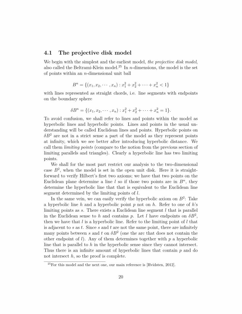
4.1 The projective disk modelWe begin with the simplest and the earliest model, the projective disk model,also called the Beltrami-Klein model.25 In n-dimensions, the model is the setof points within an n-dimensional unit ball

Bn = {(x1, x2, · · · , xn) : x21 + x2

2 + · · ·+ x2n < 1}

with lines represented as straight chords, i.e. line segments with endpointson the boundary sphere

δBn = {(x1, x2, · · · , xn) : x21 + x2

2 + · · ·+ x2n = 1}.

To avoid confusion, we shall refer to lines and points within the model ashyperbolic lines and hyperbolic points. Lines and points in the usual un-derstanding will be called Euclidean lines and points. Hyperbolic points onδB2 are not in a strict sense a part of the model as they represent pointsat infinity, which we see better after introducing hyperbolic distance. Wecall them limiting points (compare to the notion from the previous section oflimiting parallels and triangles). Clearly a hyperbolic line has two limitingpoints.

We shall for the most part restrict our analysis to the two-dimensionalcase B2, when the model is set in the open unit disk. Here it is straight-forward to verify Hilbert’s first two axioms; we have that two points on theEuclidean plane determine a line l so if those two points are in Bn, theydetermine the hyperbolic line that that is equivalent to the Euclidean linesegment determined by the limiting points of l.

In the same vein, we can easily verify the hyperbolic axiom on B2: Takea hyperbolic line h and a hyperbolic point p not on h. Refer to one of h’slimiting points as s. There exists a Euclidean line segment l that is parallelin the Euclidean sense to h and contains p. Let l have endpoints on δB2,then we have that l is a hyperbolic line. Refer to the limiting point of l thatis adjacent to s as t. Since s and t are not the same point, there are infinitelymany points between s and t on δB2 (one the arc that does not contain theother endpoint of l). Any of them determines together with p a hyperbolicline that is parallel to h in the hyperbolic sense since they cannot intersect.Thus there is an infinite amount of hyperbolic lines that contain p and donot intersect h, so the proof is complete.

25For this model and the next one, our main reference is [Hvidsten, 2012].

20

Next we need to define distance on Bn, or a metric, which is a binaryfunction that defines distance. There are certain natural conditions whichsuch a metric needs to fulfill. For all hyperbolic points x and y, we musthave

1. d(x, y) ≥ 0 with equality only when x = y.

2. d(x, y) = d(y, x).

3. (The triangle inequality) d(x, y) ≤ d(x, z) + d(z, y) for all hyperbolicpoints z.

The Euclidean metric is not sufficient in our model since it will fail thetriangle inequality; this is a consequence of the Pythagorean theorem’s failureto hold on the hyperbolic plane as it is equivalent to the parallel postulate.Therefore we need a different metric. We first have to introduce the termcross-ratio.

Definition 4.1. The cross-ratio of four collinear points a, b, x, y is

[a, b, x, y] = |a− x| · |b− y||a− y| · |b− x|

when |s− t| is the Euclidean distance between two points s and t.

The cross-ratio is an important tool in projective geometry, from which thismodel takes its name and where the following metric was first used.

Definition 4.2. Given two hyperbolic points a and b on Bn, let the limitingpoints of the hyperbolic line which they determine be x and y so that x−a−b− y. Then the hyperbolic distance between a and b is given by the metric

d(a, b) = 12 | log[b, a, x, y]|

when log signifies the natural logarithm.

The constant 12 could be any positive real number but the one we chose

happens to corresponds to −1 as the curvature of space. It is now clearto see what was meant by the boundary sphere being the set of hyperbolicpoints at infinity. We take an example on B2. Let a and b be two hyperbolicpoints on the real number line. If b approaches the point (1, 0) then the

21

hyperbolic distance between those points is limx→1

12 log s

(1−x) with s being somepositive number as long as a is any point firmly within the disk. This limitapproaches positive infinity.

It is trivial to show that our hyperbolic metric fulfills the first two metricconditions that were stated above. Proving the triangle inequality requiresmore work but a proof can be found in [McMullen, 2002, page 157].

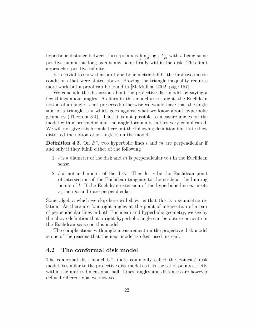
We conclude the discussion about the projective disk model by saying afew things about angles. As lines in this model are straight, the Euclideannotion of an angle is not preserved; otherwise we would have that the anglesum of a triangle is π which goes against what we know about hyperbolicgeometry (Theorem 3.4). Thus it is not possible to measure angles on themodel with a protractor and the angle formula is in fact very complicated.We will not give this formula here but the following definition illustrates howdistorted the notion of an angle is on the model.Definition 4.3. On Bn, two hyperbolic lines l and m are perpendicular ifand only if they fulfill either of the following

1. l is a diameter of the disk and m is perpendicular to l in the Euclideansense.

2. l is not a diameter of the disk. Then let s be the Euclidean pointof intersection of the Euclidean tangents to the circle at the limitingpoints of l. If the Euclidean extension of the hyperbolic line m meetss, then m and l are perpendicular.

Some algebra which we skip here will show us that this is a symmetric re-lation. As there are four right angles at the point of intersection of a pairof perpendicular lines in both Euclidean and hyperbolic geometry, we see bythe above definition that a right hyperbolic angle can be obtuse or acute inthe Euclidean sense on this model.

The complications with angle measurement on the projective disk modelis one of the reasons that the next model is often used instead.

4.2 The conformal disk modelThe conformal disk model Cn, more commonly called the Poincaré diskmodel, is similar to the projective disk model as it is the set of points strictlywithin the unit n-dimensional ball. Lines, angles and distances are howeverdefined differently as we now see.

22

Definition 4.4. On Cn, a hyperbolic line is either i) a Euclidean diameterof the unit sphere ii) a Euclidean circular arc that meets the endpoints onthe boundary sphere at Euclidean right angles.

As in the previous model, the endpoints on the sphere are considered model-wise to be points at infinity and do not belong to the model. Hence allhperbolic lines extend to infinity, which is a property we know they shouldhave. We know from Euclidean geometry the following fact; given two dis-tinct points within a circle c, there is a unique circle d that contains thosetwo points and intersect c at right angles. The circular arc of d within c isthe hyperbolic line between the two points in this model, thuse there is aunique hyperbolic line that contains any two distinct points so Hilbert’s firsttwo axioms are fulfilled. Therefore we can borrow the same definitions oflimiting points from the last model, which enables us to define a very similarmetric as before:

Definition 4.5. Given two hyperbolic points a and b on Cn, let the limitingpoints of the hyperbolic line which they determine be x and y so that x−a−b− y. Then the hyperbolic distance between a and b is given by the metric

d(a, b) = |log[b, a, x, y]| .

We will now show that there exists an isomorphism between the projectiveand the conformal disk models, that is a map that preserves points, lines,angles and the distance function. As usual, we consider the case when n = 2so we consider the map from B2 to C2. Let the unit sphere be given. Thenlet the unit disk within the the sphere contain the projective disk. Projectorthogonally any hyperbolic point P on the disk from the north pole of thesphere onto the bottom hemisphere, yielding point Q, and then project Qstereographically from the north pole back onto the unit disk, yielding pointP ′ on the conformal disk. We see that P ′ is a unique point given the pointP and we let F be the function that takes the point P and returns P ′. Asorthogonal and stereographic projections are bijective, so is F , and thus theinverse of F , denoted F ′, is a well-defined function that maps the conformaldisk to the projective disk. If the Cartesian coordinates of P is (x, y), thenwe have that

F (x, y) =(

x

1 +√

1− x2 − y2 ,y

1 +√

1− x2 − y2

)

23

Figure 2

and

F ′(x, y) =(

2x1 + x2 + y2 ,

2y1 + x2 + y2

)Clearly F preserves the notions of points between the models. Using theproperties of stereographic and orthogonal projections, we will also see thatthe F preserves the lines and angles, for details see [Hvidsten, 2012]. Wewill sketch a method that shows the distance function is preserved. Let dBand dC be the distance metrics on the projective and conformal disk modelrespectively. Then we want to show that for two hyperbolic points P and Qon the projective disk, dB(P,Q) = dC(F (P ), F (Q)). Assume without loss ofgenerality that P = (x1, 0) and Q = (x2, 0) are on the real number line andthat x1 < x2. Then

dB(P,Q) = 12 log |x2 − (−1)| · |x1 − 1|

|x2 − 1| · |x1 − (−1)| = 12 log (x2 + 1) · (x1 − 1)

(x2 − 1) · (x1 + 1)

We have that that

F (P ) = x1

1 +√

1− x21

, 0 , F (Q) =

x2

1 +√

1− x22

, 0

so

24

dC(F (P ), F (Q)) = log

∣∣∣∣∣∣∣∣(

x21+√

1−x22

+ 1)·(

x11+√

1−x21− 1

)(

x21+√

1−x22− 1

)·(

x11+√

1−x21

+ 1)∣∣∣∣∣∣∣∣

which after some laborious algebra simplifies to 12 log (x2+1)·(x1−1)

(x2−1)·(x1+1) = dB(P,Q).Thus we have that the isomorphism between the two models exists, so

there is hyperbolic geometry on the conformal disk model. It follows thatthe hyperbolic axiom is valid here, but we nevertheless sketch a proof (onlyfor C2). Let a hyperbolic line h and a hyperbolic point p not on h be given.Call the limiting points of h x and y. Then there are two distinct hyperboliclines determined by x and p, and y and p, that contain p and do not intersecth at any point. Furthermore, there are infinite such lines; let l be the linedetermined by p and x and let z be its limiting point that is not x. Thenany point between z and x on the bounding circle, which are infinitely many,determines with p a line that contains p and does not intersect h.

As the name of the model suggests, the angle measure of the hyperbolicplane is preserved. To find the angle at the point of intersection of twohyperbolic lines, we find the Euclidean tangents to the corresponding circulararcs at the point and calculate the angle determined by the tangents in theusual Euclidean fashion. We now see why we skipped giving an angle formulain the previous section; the easiest way to calculates angles on the projectivedisk model is to project first to the conformal disk and then use the aboveprocedure.

4.3 The hyperboloid modelAs we have mentioned, there were complications in the previous two mod-els; either angles or lines are distorted. Trying to solve this resembles theproblem of depicting a globe on a flat map, which is not possible withoutsome distortion. Like in the case of the globe, we can avoid the compli-cations we encountered by considering the geometry on a two-dimensionalsurface in three-dimensional space, or to generalize, a n-dimensional surfaceembedded in n+1-dimensional space, when the surface has constant nega-tive curvature. But as mentioned in the second section, no such surface canpossibly exist in Euclidean 3-space, so in order to find a suitable model forgeneral n-dimensional hyperbolic geometry we need to work in a different in-ner product space: Lorentzian n-space, which we denote as Ln, a real vector

25

space with properties that will now be defined.26 If x and y are vectors inLn, their inner product is defined as the real number

x ◦ y = −x1y1 + x2y2 + · · ·+ xnyn

.From there we define the norm of a vector x to be the complex number

||x|| = (x ◦ x) 12

which, being the square root of a real number, is either real and positive, zeroor strictly imaginary. As a sphere with a positive real radius has constantpositive curvature on its surface, it should make some sense that a spherewith imaginary radius has constant negative curvature on its surface. Thiskind of an object exists in Lorentzian space and therefore, for our model ofn-dimensional hyperbolic geometry, we would like to take the surface of an+1-dimensional sphere of unit imaginary radius, which is

P n = {x ∈ Ln+1 : ||x||2 = −1}.which we see that is the set of all the vectors (i.e. points) x = (x1, x2, · · · , xn+1)that fulfill the equation x2

1 − x22 − · · · − x2

n+1 = 1. This is a disconnected setsince the equation describes a two-sheeted hyperboloid, so for our model weonly take the positive sheet of P n, that is we require x1 > 0. We denote themodel as Hn.

The next step is to define the hyperbolic lines of Hn:

Definition 4.6. A hyperbolic line in Hn is the intersection of Hn with theEuclidean plane spanned by two points on Hn and the origin.

A hyperbolic line is in fact a branch of a hyperbola. Unlike the other models,there is no space at infinity in H2 so visually, hyperbolic lines go indefinitelyfar up on the hyperboloid.

We can now verify that Hilbert’s first two axioms of hyperbolic geometryare true in this model.

Theorem 4.7. Any two distinct points on H2 determine a line.26The following definitions of the inner product and norm in Lorentzian space and

the definition, distance and geodesics of the hyperboloid model follow approximately thedevelopment given by [Ratcliffe, 1994].

26

Figure 3: H2 is the points on this hyperboloid. The hyperboloid is asymp-totically bounded by the cone C2, which is the set of vectors with x1 > 0and the norm zero.

Proof. We begin by showing that the distinct points x, y onH2 and the originare noncollinear (in the Euclidean sense). Assume that they are collinear.As x and y are on H2, we have that x = (

√x2

2 + x23 + 1, x2, x3) and y =

(√y2

2 + y23 + 1, y2, y3). Since they are collinear with the origin, x and y are

a scalar multiple of each other, so there must exist some real number k sothat k(

√x2

2 + x23 + 1, x2, x3) = (

√y2

2 + y23 + 1, y2, y3) so k ·

√x2

2 + x23 + 1 =√

y22 + y2

3 + 1, k · x2 = y2 and k · x3 = y3. By making substitutions we get

k ·√x2

2 + x23 + 1 =

√(k · x2)2 + (k · x3)2 + 1 =

√k2 · x2

2 + k2 · x23 + 1

which implies that

k2 · (x22 + x2

3 + 1) = k2 · x22 + k2 · x2

3 + 1

⇐⇒ k2 · x22 + k2 · x2

3 + k2 = k2 · x22 + k2 · x2

3 + 1 ⇐⇒ k2 = 1

and as k cannot be negative (since (x1 > 0 per definition), we have that k = 1and hence x = y, which is a contradiction. Hence x, y and the origin are

27

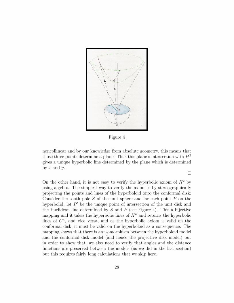
Figure 4

noncollinear and by our knowledge from absolute geometry, this means thatthose three points determine a plane. Thus this plane’s intersection with H2

gives a unique hyperbolic line determined by the plane which is determinedby x and y.

On the other hand, it is not easy to verify the hyperbolic axiom of H2 byusing algebra. The simplest way to verify the axiom is by stereographicallyprojecting the points and lines of the hyperboloid onto the conformal disk:Consider the south pole S of the unit sphere and for each point P on thehyperbolid, let P ′ be the unique point of intersection of the unit disk andthe Euclidean line determined by S and P (see Figure 4). This a bijectivemapping and it takes the hyperbolic lines of Hn and returns the hyperboliclines of Cn, and vice versa, and as the hyperbolic axiom is valid on theconformal disk, it must be valid on the hyperboloid as a consequence. Themapping shows that there is an isomorphism between the hyperboloid modeland the conformal disk model (and hence the projective disk model) butin order to show that, we also need to verify that angles and the distancefunctions are preserved between the models (as we did in the last section)but this requires fairly long calculations that we skip here.

28

As stated earlier, the main advantage of this model is that it is free ofdistortions. The hyperbolic line segment between two points on Hn is theshortest path on the surface of a hyperboloid in Ln+1 and the angle definedby line segments matches the general definition of an angle in Lorentzianspace. The former can be realized by using this definition:

Definition 4.8. The Lorentzian distance between two vectors x and y isthe complex number ||x − y||. The hyperbolic distance between hyperbolicpoints x and y is the real number dH(x, y) = arccosh(−x ◦ y).

The hyperbolic distance function is a metric since it satisfies all the necessaryconditions. Only the triangle inequality is nontrivial to show but a proofusing Lorentz transformations can be found in [Ratcliffe, 1994, page 66]. Thisdefinition of distance completes the description of the hyperboloid model.

We conclude the paper by discussing briefly the relation of the model tomathematical physics. L4 is called Minkowski space-time27 and is the space-time setting for special relativity. The vectors of Minkowski space-time arecalled events. An event x is said to be light-like if ||x|| = 0; the set ofsuch events forms two hypercones, called light cones, defined by the equationx2

1 = x22 +x2

3 +x44. The events inside the light cones (when x2

1 < x22 +x2

3 +x44)

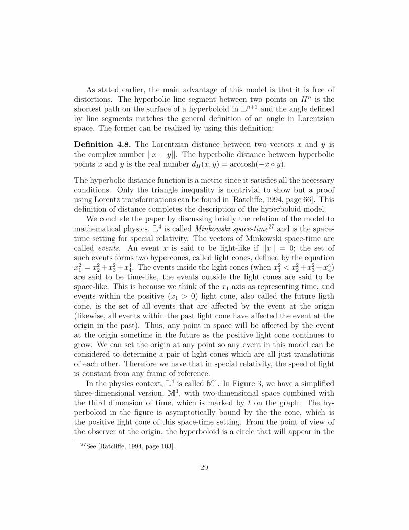
are said to be time-like, the events outside the light cones are said to bespace-like. This is because we think of the x1 axis as representing time, andevents within the positive (x1 > 0) light cone, also called the future ligthcone, is the set of all events that are affected by the event at the origin(likewise, all events within the past light cone have affected the event at theorigin in the past). Thus, any point in space will be affected by the eventat the origin sometime in the future as the positive light cone continues togrow. We can set the origin at any point so any event in this model can beconsidered to determine a pair of light cones which are all just translationsof each other. Therefore we have that in special relativity, the speed of lightis constant from any frame of reference.

In the physics context, L4 is called M4. In Figure 3, we have a simplifiedthree-dimensional version, M3, with two-dimensional space combined withthe third dimension of time, which is marked by t on the graph. The hy-perboloid in the figure is asymptotically bound by the the cone, which isthe positive light cone of this space-time setting. From the point of view ofthe observer at the origin, the hyperboloid is a circle that will appear in the

27See [Ratcliffe, 1994, page 103].

29

future with a centre at the origin. Its radius will increase faster than thespeed of light.28

28See [Reynolds, 1993, page 443-444].

30

BibliographyAdler, I. (1987). Some philosophical implications of modern mathematics.Science & Society 51, no.2, 154–169.

Arcozzi, N. (2012). Mathematicians in Bologna 1861-1960, Chapter 1: Bel-trami’s Models of Non-Euclidean Geometry, pp. 1–31. Birkhauser.

Cannon, J. W., W. J. Floyd, R. Kenyon, and W. R. Parry (1997). Hyperbolicgeometry. MSRI Publications 31, 59–115.

Euclid (1908). The Thirteen Books of Euclid’s Elements, translated from thetext of Heiberg with introduction and commentary by T.L. Heath, Volume I.Cambridge University Press.

Gray, J. (2007). Worlds Out of Nothing: A Course in the History of Geometryin the 19th Century. Springer-Verlag London Limited.

Greenberg, M. J. (1993). Euclidean and non-Euclidean geometry: Develop-ment and History (3 ed.). W. H. Freeman and Company.

Greenberg, M. J. (2010). Old and new results in the foundations of Ele-mentary plane Euclidean and non-Euclidean geometries. The AmericanMathematical Monthly 117, 198–219.

Hartshorne, R. (2000). Geometry: Euclid and Beyond. Springer.

Hilbert, D. (1950). The Foundations of Geometry, English translation by E.J. Townsend. The Open Court Publishing Company,.

Hvidsten, M. (2012). Exploring geometry. Draft: October 18, 2012.

Legendre, A. (1841). Elements of Geometry: Translated from the French.Hilliard, Gray, and Company.

Lobachevsky, N. I. (2010). Pangeometry. European Mathematical Society.

McMullen, C. T. (2002). Coxeter groups, Salem numbers and the Hilbertmetric. Publications Mathématiques de l’Institut des Hautes Études Scien-tifiques 95, 151–183.

Milnor, J. (1982). Hyperbolic geometry: The first 150 years. Bulletin of theAmerican Mathematical Society 6.

31

Mueller, I. (1969). Euclid’s elements and the axiomatic method. The BritishJournal for the Philosophy of Science 20, 289–309.

Penrose, R. (2004). Road to Reality. Jonathan Cape.

Proclus (1970). Proclus: A Commentary on the First Book of Euclid’s Ele-ments. Princeton University Press.

Ratcliffe, J. G. (1994). Foundations of Hyperbolic Manifolds. Springer-Verlag.

Reynolds, W. F. (May, 1993). Hyperbolic geometry on a hyperboloid. TheAmerican Mathematical Monthly 100, 442–455.

Stillwell, J. (1996). Sources of Hyperbolic Geometry. American MathematicalSociety.

Taimina, D. and D. Henderson (2005). How to use history to clarify commonconfusions in geometry. Mathematical Association of America Notes.

Tarski, A. and S. Givant (1999). Tarski’s system of geometry. Bulletin ofSymbolic Logic 5, 175–214.

Trudeau, R. J. (2001). The Non-Euclidean Revolution. Birkhäuser Boston.

Weisstein, E. W. (2005). Gauss-Bonnet formula. From MathWorld–A Wolfram Web Resource. http://mathworld.wolfram.com/Gauss-BonnetFormula.html.

32