Hydrologie spatiale :Développement d'applications pour l'utilisation ...
284
HAL Id: tel-00080744 https://tel.archives-ouvertes.fr/tel-00080744 Submitted on 20 Jun 2006 HAL is a multi-disciplinary open access archive for the deposit and dissemination of sci- entific research documents, whether they are pub- lished or not. The documents may come from teaching and research institutions in France or abroad, or from public or private research centers. L’archive ouverte pluridisciplinaire HAL, est destinée au dépôt et à la diffusion de documents scientifiques de niveau recherche, publiés ou non, émanant des établissements d’enseignement et de recherche français ou étrangers, des laboratoires publics ou privés. Hydrologie spatiale :Développement d’applications pour l’utilisation de la télédétection sur les grands bassins fluviaux Frédéric Frappart To cite this version: Frédéric Frappart. Hydrologie spatiale :Développement d’applications pour l’utilisation de la télédé- tection sur les grands bassins fluviaux. Autre. Université Paul Sabatier - Toulouse III, 2005. Français. <tel-00080744>
Transcript of Hydrologie spatiale :Développement d'applications pour l'utilisation ...

HAL Id: tel-00080744https://tel.archives-ouvertes.fr/tel-00080744
Submitted on 20 Jun 2006
HAL is a multi-disciplinary open accessarchive for the deposit and dissemination of sci-entific research documents, whether they are pub-lished or not. The documents may come fromteaching and research institutions in France orabroad, or from public or private research centers.
L’archive ouverte pluridisciplinaire HAL, estdestinée au dépôt et à la diffusion de documentsscientifiques de niveau recherche, publiés ou non,émanant des établissements d’enseignement et derecherche français ou étrangers, des laboratoirespublics ou privés.
Hydrologie spatiale :Développement d’applications pourl’utilisation de la télédétection sur les grands bassins
fluviauxFrédéric Frappart
To cite this version:Frédéric Frappart. Hydrologie spatiale :Développement d’applications pour l’utilisation de la télédé-tection sur les grands bassins fluviaux. Autre. Université Paul Sabatier - Toulouse III, 2005. Français.<tel-00080744>

UNIVERSITE TOULOUSE III - PAUL SABATIER
U.F.R. Physique - Chimie – Automatique
THESE
pour obtenir le grade de
DOCTEUR DE L’UNIVERSITE TOULOUSE III
Discipline :
Géophysique et Télédétection spatiale
présentée par
Frédéric FRAPPART
le 30 janvier 2006
Directrices de thèse : Anny CAZENAVE et Frédérique SEYLER
JURY
Franck ROUX (LA, Univ. P. Sabatier, Toulouse) Président
Catherine PRIGENT (Obs. de Paris Meudon, Paris) Rapporteur
Patrick VINCENT (IFREMER, Paris) Rapporteur
Anny CAZENAVE (LEGOS-GRGS/CNES, Toulouse) Directrice de thèse
Frédérique SEYLER (IRD, LMTG/HYBAM, Toulouse) Co-directrice de thèse
Jean-Loup GUYOT (IRD, LMTG/HYBAM, Toulouse) Examinateur
Jérôme BRUNIQUEL (Alcatel-Space, Toulouse) Invité
Hervé DOUVILLE (Météo France, Toulouse) Invité
Philippe ESCUDIER (CLS, Toulouse) Invité
Travaux effectués au LEGOS et au LMTG
Observatoire Midi-Pyrénées
14, Avenue Edouard BELIN
31400 Toulouse, France
Hydrologie spatiale :
Développement d’applications pour l’utilisation de la télédétection sur les
grands bassins fluviaux


Hydrologie spatiale : Développement d’outils méthodologiques pour l’utilisation de la télédétection sur les
grands bassins fluviaux
Résumé
3
RESUME
Les techniques de télédétection spatiale constituent un apport majeur pour l’étude des
variations de masses d’eau dans les grands bassins fluviaux, en permettant un suivi homogène
de ces fluctuations dans l’espace et dans le temps.
L’objectif de cette thèse a été de développer de nouvelles applications hydrologiques au
moyen des mesures spatiales acquises par différents types de mission satellitaire : altimétrie
radar, imagerie satellitaire, gravimétrie spatiale. L’altimétrie spatiale offre la possibilité
d’étudier les variations de niveau d’eau des grands fleuves, des lacs et des zones d’inondation,
garantissant ainsi une surveillance continue et globale des eaux de surface. Elle donne aussi
accès à des produits hydrologiques nouveaux comme le profil hydrologique ou la pente des
fleuves. Elle permet en outre de définir des réseaux limnimétriques nivelés, dont les stations
peuvent être définis tant sur les fleuves que sur les zones d’inondation, complémentaires des
réseaux in-situ. Combinée à l’imagerie spatiale, l’altimétrie satellitaire a été utilisée pour
déterminer les variations de volume d’eau dans les grands bassins fluviaux. Ces paramètres
revêtent, en effet, une importance fondamentale pour les hydrologues car le premier est à la
base des études hydrodynamiques et le second apporte des contraintes sur la répartition des
masses d’eau entre zones inondées et réseau hydrographique, avec des applications au
transport des sédiments et à la disponibilité des ressources en eau à l’échelle régionale. Des
exemples d’utilisation de ces techniques sont présentés pour les bassins amazoniens et du
Mékong. La mission de gravimétrie spatiale GRACE, lancée en mars 2002, fournit, quant à
elle, les variations spatio-temporelles des stocks d’eaux continentales (eau des sols et manteau
neigeux) et de paramètres hydrologiques dérivés comme l’évapotranspiration. Une analyse de
l’évolution des stocks d’eau et de neige est présentée à partir des premiers géoïdes mensuels
issus de la mission GRACE, aux échelles globale et régionale, ainsi que le calcul du
paramètre d’évapotranspiration, à l’échelle du bassin versant. Ces résultats sont comparés à la
variation des volumes d’eau de surface obtenue précédemment pour le bassin du Mékong.
Mots clés: Télédétection spatiale, Altimétrie satellitaire, Imagerie spatiale, Gravimétrie
Spatiale, Cycle de l’eau, Hydrologie continentale.

Hydrologie spatiale : Développement d’outils méthodologiques pour l’utilisation de la télédétection sur les
grands bassins fluviaux
Résumé
4
SUMMARY
Remote sensing can be considered as an important tool for studying the variations of water
masses in large river basins due to a homogeneous sampling both in space and time. The
objective of this PhD thesis was to develop new hydrological applications using
measurements acquired by various types of satellite mission: radar altimetry, satellite
imagery, gravimetry from space. Space altimetry is commonly used to study time variations
of water level of large rivers, lakes and flooded zones. New hydrological products such as
hydrological profiles or river slopes. Levelled limnimetric networks can thus be defined, with
gauge stations on the rivers as welle as on the flooded zones. Used in combination with
imagery from space, satellite altimetry can be used to determine surface water volume
variations in large river basins. These parameters are fundamental for hydrologists because
hydrological profiles are necessary for hydrodynamic studies and distribution of water volume
variations constrains the distribution of water masses between flooded zones and
hydrographic network. Examples of use of these techniques are presented for the Amazon
and the Mekong basins. In March 2002, a new generation of gravity missions was launched:
the Gravity Recovery and Climate Experiment (GRACE) space mission. The objective of
GRACE is to measure spatio-temporal variations of the gravity field with an unprecedented
resolution and precision, over time scales ranging from a few months to several years. As
gravity is an integral of mass, these spatio-temporal gravity variations represent horizontal
mass redistributions only to the extent they are assumed to be caused by surface water
changes. On time scales from months to decades, mass redistribution mainly occurs inside the
surface fluid envelopes (oceans, atmosphere, ice caps, continental reservoirs) and is related to
climate variability. An analysis of the evolution of water and snow mass is presented using
the first monthly geoids from the GRACE mission, at global and regional scales, as well as
the estimation of evapotranspiration rate at basin scale. These results are compared with
surface water volume variations previously obtained for the Mekong basin.
Keywords : Remote sensing, Altimetry, Imagery and Gravimetry from space, Hydrological
cycle, Land waters.

Hydrologie spatiale : Développement d’outils méthodologiques pour l’utilisation de la télédétection sur les
grands bassins fluviaux
Remerciements
5
REMERCIEMENTS
Je tiens, tout d’abord, à remercier très chaleureusement mes directrices de thèse, Anny
Cazenave et Frédérique Seyler, pour la qualité de leur encadrement tant sur le plan
scientifique qu’humain, leurs encouragements, leur enthousiasme et leur grande disponibilité
au cours de ces trois années. Merci Anny, d’avoir assuré avec un dynamisme sans faille
l’encadrement de cette thèse et d’avoir su me communiquer rigueur scientifique et passion
pour la géophysique. Merci Frédérique de m’avoir fait profiter de tes connaissances du bassin
amazonien, de m’avoir intégré au projet HYBAM et également pour ton aide précieuse tout
au long de ces trois ans. L’escapade sur les eaux limoneuses du Rio Branco, au cœur de
l’Amazonie brésilienne, demeure un souvenir inoubliable. Je vous exprime toute ma
reconnaissance pour la confiance que vous m’avez accordée au cours de ces trois années.
Je souhaite aussi remercier tout particulièrement Guillaume Ramillien et Benoît Legrésy pour
leur patience, leur capacité d’écoute, leurs réflexions constructives et leur soutien sans faille.
Merci à Stéphane Calmant, Nelly Mognard, Kien Do Minh, Thuy Le Toan du CESBIO qui
ont su me faire profiter de leur connaissance de l’altimétrie satellitaire, des régions boréales et
du bassin du Mékong. Un grand merci à Alexei, Juan, Julien, Mathilde, Sylvain.
Je tiens à remercier également Franck Roux pour m’avoir fait l’honneur de présider mon jury
de thèse, Catherine Prigent et Patrick Vincent pour avoir accepté d’en être les rapporteurs,
Jean-Loup Guyot pour l’avoir examiné, Jérôme Bruniquel, Hervé Douville et Philippe
Escudier pour avoir bien voulu en faire partie.
Ces travaux de thèse, financés par le Centre National d’Etudes Spatiales et Alcatel/Alenia
Space, ont été menés au Laboratoire d’Etudes en Géophysique et Océanographie Spatiales et
au Laboratoire des Mécanismes et Transferts en Géologie, de l’Observatoire Midi-Pyrénées, à
Toulouse. Je remercie leur directeur, Patrick Monfray et Bernard Dupré, de m’y avoir
accueilli durant ces trois années.
Les personnes qui contribuent à rendre le LEGOS vivant et convivial sont trop nombreuses
pour être toutes citées. Elles se reconnaîtront parmi celles à qui j’exprime ma profonde
gratitude et mes sincères remerciements. Merci aux membres de l’équipe GOHS.
Merci à Pascal et Guillaume pour la bonne ambiance qui a régné au cours de ces trois ans
dans les bureaux 14 puis D 002. Merci aux pilotariak, basketteurs, grimpeurs et pyrénéistes de
l’OMP et du CNES pour l’anima sana in corpore sano.
Eun grand mèrcie à mes pathents, à ma fanmil’ye, de Nouormandie et d’ailleurs, à m’s amins.
Ce manuscrit leur est dédié.

Hydrologie spatiale : Développement d’outils méthodologiques pour l’utilisation de la télédétection sur les
grands bassins fluviaux
Remerciements
6

Hydrologie spatiale : Développement d’outils méthodologiques pour l’utilisation de la télédétection sur les
grands bassins fluviaux
Table des matières
7
TABLE DES MATIERES
Introduction ......................................................................................11
Chapitre 1 : Le cycle de l’eau...........................................................15
1. L’eau continentale..................................................................................... 16
1.1 Le cycle hydrologique global ............................................................................... 16
1.2 Les eaux continentales ......................................................................................... 17
2. Contraintes observationnelles d’un milieu complexe............................... 19
3. Apport de la télédétection spatiale............................................................ 21
4. Le suivi des eaux continentales par altimétrie satellitaire ........................ 21
Chapitre 2 : L’altimétrie satellitaire .................................................25 1. L’altimétrie satellitaire.............................................................................. 26
1.1 L’altimètre radar................................................................................................... 26
1.2 Le principe de l’altimétrie satellitaire .................................................................. 27
2. L’altimétrie satellitaire.............................................................................. 28 2.1 Principe de la mesure radar .................................................................................. 28
2.2 Effet géométrique et échantillonnage géographique........................................... 30
2.2 Résolution au nadir et échantillonnage temporel ................................................. 31
3. Estimation de la hauteur altimétrique ....................................................... 32 3.1 Principe................................................................................................................. 32
3.2 L’orbite des satellites ........................................................................................... 32
3.3 Les corrections géophysiques et environnementales à appliquer à la mesure
altimétrique........................................................................................................................ 33
3.4 La correction de marée solide .............................................................................. 34
3.5 La correction de marée polaire............................................................................. 35
4. Les différentes missions d’altimétrie satellitaire ...................................... 35 4.1 La mission altimétrique Topex/Poséidon............................................................. 36
4.2 La mission altimétrique Jason-1........................................................................... 37
4.3 Les missions altimétriques ERS-1&2 .................................................................. 38
4.4 La mission altimétrique ENVISAT...................................................................... 38
Chapitre 3 : Le traitement des échos radar – Cas des surfaces
continentales.....................................................................................41 1. Introduction............................................................................................... 42
2. Traitement des échos radar ....................................................................... 42 2.1 Principe................................................................................................................. 42
2.2 Traitement des échos océaniques ......................................................................... 43
3. Les formes d’onde altimétriques sur les eaux continentales .................... 44
4. Les principaux algorithmes développés pour l’étude des terres émergées
…………………………………………………………………………...47

Hydrologie spatiale : Développement d’outils méthodologiques pour l’utilisation de la télédétection sur les
grands bassins fluviaux
Table des matières
8
4.1 Les méthodes de seuillage.................................................................................... 47
4.2 Les algorithmes analytiques : l’exemple d’Ice-2 ................................................. 49
4.3 Les méthodes de reconnaissance des formes ....................................................... 50
5. Les limitations de l’altimétrie sur les eaux continentales......................... 51 5.1 Décrochage de l’altimètre .................................................................................... 51
5.2 Accrochage de l’altimètre .................................................................................... 52
5.3 Erreurs dues à la pente ......................................................................................... 53
6. Conclusion ................................................................................................ 54
Chapitre 4 : De la mesure altimétrique aux niveaux d’eau sur les
continents .........................................................................................57 1. Introduction............................................................................................... 58
2. Les produits altimétriques......................................................................... 58
3. Construction des séries temporelles de hauteur d’eau.............................. 59 3.1 Sélection géographique ........................................................................................ 59
3.2 Sélection des mesures valides .............................................................................. 60
3.3 Séries temporelles de hauteur d’eau..................................................................... 60
4. Application à la validation des hauteurs d’eau déduites des mesures
d’ENVISAT...................................................................................................... 63 4.1 Choix de la zone d’étude...................................................................................... 63
4.2 Comparaison avec les mesures in-situ ................................................................. 64
4.3 L’exemple de la várzea de Curuai........................................................................ 66
5. Conclusion ................................................................................................ 69
Chapitre 5 : Estimation des profils hydrologiques des fleuves au
moyen de l’altimétrie satellitaire......................................................71
1. Introduction............................................................................................... 72
2. Intérêt de l’estimation des profils hydrologiques ..................................... 72
3. Profil hydrologique du Rio Negro et de ses affluents............................... 73 3.1 Données utilisées.................................................................................................. 73
3.2 Profils longitudinaux ............................................................................................ 74
4. Comparaison avec d’autres sources de données ....................................... 77 4.1 Comparaison avec des mesures GPS ................................................................... 77
4.2 Comparaison avec les sorties du modèle Muskingum-Cunge ............................. 78
5. Conclusion...............................................................................79
Chapitre 6 : Variations de volume d’eau de surface dans les grands
bassins fluviaux – Etude de la synergie altimétrie
satellitaire/imagerie spatiale.............................................................81
1. Introduction............................................................................................... 82
2. Méthode d’estimation des variations de volume d’eau ............................ 83 2.1 Le bassin du Rio Negro........................................................................................ 83
2.2 Identification des zones en eau............................................................................. 84

Hydrologie spatiale : Développement d’outils méthodologiques pour l’utilisation de la télédétection sur les
grands bassins fluviaux
Table des matières
9
2.3 Les cartes de hauteur d’eau .................................................................................. 86
2.4 Estimation des variations de volume d’eau.......................................................... 87
2.5 Résultats ............................................................................................................... 87
2.6 Article “Floodplain water storage in the Negro River basin estimated from
microwave remote sensing of inundation area and water levels “ .................................... 88
3. Variations inter-annuelles de volume d’eau de surface dans la partie avale
du bassin du Mékong...................................................................................... 102 3.1 Caractéristiques hydrologiques de la zone étudiée ............................................ 102
3.2 Délimitation des zones inondées ........................................................................ 103
3.3 Cartes de hauteur d’eau ...................................................................................... 105
3.4 Estimation des variations de volume d’eau........................................................ 107
3.5 Résultats ............................................................................................................. 107
3.6 Article “Water volume change in the lower Mekong basin from satellite altimetry
and other remote sensing data”........................................................................................ 109
4. Conclusion .............................................................................................. 139
Chapitre 7 : GRACE et l’hydrologie continentale .........................141 1. Le bilan hydrique du bassin versant ....................................................... 142
2. Les modèles hydrologiques globaux....................................................... 143
2.1 Le modèle WGHM............................................................................................. 144
2.2 Le modèle LaD................................................................................................... 144
2.3 Le modèle ORCHIDEE...................................................................................... 144
2.4 Le système d’assimilation GLDAS.................................................................... 144
3. La mission de gravimétrie spatiale GRACE........................................... 145
3.1 Les objectifs ....................................................................................................... 145
3.2 Les géoïdes mensuels ......................................................................................... 146
4. Application à l’hydrologie globale ......................................................... 147
4.1 Travaux antérieurs.............................................................................................. 148
4.2 Méthodologie ..................................................................................................... 148
5. Résultats .................................................................................................. 149
5.1 Validation de la méthode inverse ....................................................................... 149
5.2 Estimation des masses d’eaux continentales ...................................................... 169
5.3 Estimation des masses de neige aux latitudes boréales...................................... 173
5.4 Estimation de l’évapotranspiration à l’échelle du basin versant ........................ 179
6. Discussion – Perspectives ....................................................................... 196
Conclusion......................................................................................197
Bibliographie..................................................................................201
Annexe 1 ........................................................................................217
Annexe 2 ........................................................................................253

Hydrologie spatiale : Développement d’outils méthodologiques pour l’utilisation de la télédétection sur les
grands bassins fluviaux
Table des matières
10
Annexe 3 ........................................................................................267

Hydrologie spatiale : Développement d’outils méthodologiques pour l’utilisation de la télédétection sur les
grands bassins fluviaux
Introduction
11
INTRODUCTION
Les réservoirs hydrologiques continentaux ne représentent qu’une fraction de l’eau sur Terre
(de l’ordre de 0,025 %), mais ont cependant un rôle primordial pour la vie sur Terre et dans la
dynamique du climat, en raison de leur situation à l’interface des continents et de
l’atmosphère. Si l’on exclut les calottes polaires, l’eau douce est stockée dans les différents
réservoirs que sont le manteau neigeux, les glaciers, les aquifères, la zone racinaire, qui se
situe dans les premiers mètres du sol, et les eaux de surface qui comprennent fleuves et
rivières, lacs, retenues d’eau dues à l’activité humaine (lacs de barrage, réservoirs pour
l’irrigation,…) et zones humides. Les eaux continentales participent aux échanges avec
l’atmosphère et les océans au travers des flux de masse horizontaux et verticaux (évaporation,
transpiration, ruissellement).
La pression anthropique et les besoins humains en alimentation conduisent l’homme à
mobiliser la majeure partie de l’eau disponible pour ses besoins et activités, et principalement
pour la pratique d’une agriculture irriguée. Néanmoins, cette ressource, nécessaire à toute vie,
est bien souvent rare dans de vastes zones de la biosphère continentale et soumise aux
changements climatiques pouvant conduire soit à l’aridification et à la désertification, soit à
un fort développement du couvert végétal. Le cycle hydrologique continental demeure,
malgré tout, l’une des composantes les moins bien connues du système climatique. De
nombreux processus restent, en effet, difficilement modélisables en raison de leur complexité.
En outre, les réseaux hydrologiques nationaux, en charge du suivi continu des fluctuations du
niveau des fleuves ont vu leur nombre fortement diminuer ces dernières années dans certains
pays en voie de développement et dans les pays de l’ex-URSS, en raison du coût nécessaire à
leur entretien.
Dans ce contexte, la télédétection spatiale revêt un intérêt particulier pour la veille
hydrologique et la gestion des risques d’inondation. A l’heure actuelle, plusieurs axes ont été
retenus dans l’application de la télédétection spatiale à l’hydrologie : la délimitation des zones
d’inondation par imagerie satellitaire, le suivi des variations de niveau d’eau sur les fleuves et
les zones d’inondation par altimétrie et interférométrie radars, l’estimation des stocks d’eau
sur les continents par gravimétrie spatiale, la mesure de l’humidité des sols au moyen des
micro-ondes passives, la mesure du déplacement des eaux de surface par interférométrie
radar. En complément des observations in-situ et de la modélisation hydrologique, la
télédétection satellitaire offre l’opportunité d’améliorer, de manière non négligeable, la
compréhension des processus hydrologiques à l’œuvre dans les grands bassins fluviaux, leur

Hydrologie spatiale : Développement d’outils méthodologiques pour l’utilisation de la télédétection sur les
grands bassins fluviaux
Introduction
12
influence sur la variabilité climatique, la géodynamique ou leurs implications socio-
économiques. L’utilisation combinée des modèles hydrologiques, des observations in-situ et
des mesures satellitaires, lesquelles offrent une couverture géographique globale et une
répétitivité temporelle importante, continue dans le temps, est nécessaire à la description des
variations de masse d’eau souterraine et de surface.
Ce manuscrit se compose de sept chapitres dont le premier est consacré à la présentation du
cycle de l’eau à la surface de la Terre. Face à la diminution du nombre de réseaux
limnimétriques, la télédétection spatiale s’avère être un des outils les plus appropriés pour la
caractérisation du cycle hydrologique, tant à l’échelle globale que régionale. Nous
reviendrons sur les méthodes développées dans le cadre de travaux antérieurs et présenteront
les principaux résultats obtenus à l’aide de différents capteurs, dont les altimètres radars.
Le deuxième chapitre présente l’altimétrie satellitaire, son principe général et divers aspects
de physique de la mesure en milieu océanique. Les principales missions altimétriques
actuelles (Topex/Poseidon, ERS-1&2, Jason-1, ENVISAT) y sont présentées.
Le troisième chapitre décrit le traitement des échos radar permettant d’estimer les paramètres
physiques (hauteur altimétrique, section efficace radar) issues du signal altimétrique ainsi que
les spécificités liées à l’utilisation de l’altimétrie satellitaire en domaine continental.
La méthode permettant de passer de la mesure altimétrique aux niveaux d’eau sur les zones
humides est expliquée dans le chapitre 4 et validée au moyen de quelques exemples pris sur le
bassin amazonien.
La qualité des mesures altimétriques pour le suivi des eaux de surface a permis de développer
des applications hydrologiques de l’altimétrie satellitaire comme l’estimation du profil
longitudinal des fleuves et le calcul de variations de volume d’eau par combinaison de
l’imagerie radar et de l’altimétrie. La présentation de ces méthodes fait l’objet des chapitres 5
et 6.
Le chapitre 7 est consacré à l’application à l’hydrologie des mesures gravimétriques
effectuées par la mission GRACE. Les variations locales du champ de gravité sont le reflet
des redistributions de masses d’eau dans l’enveloppe de la Terre. Il est ainsi possible de suivre
l’évolution des stocks d’eau à l’échelle du globe, de neige aux hautes latitudes ou encore
d’estimer l’évapotranspiration à l’échelle des grands bassins fluviaux.
Pour terminer, trois annexes viennent compléter ce manuscrit. L’annexe 1 contient le rapport
de la campagne de mesures hydrologiques réalisées sur le Rio Branco en novembre 2003.
L’annexe 2 présente les premiers résultats de validation des mesures de l’altimètre
d’ENVISAT pour le suivi des eaux continentales, sur le bassin amazonien. Dans l’annexe 3,

Hydrologie spatiale : Développement d’outils méthodologiques pour l’utilisation de la télédétection sur les
grands bassins fluviaux
Introduction
13
sont regroupés des résultats concernant l’établissement d’une relation hauteur-débit à partir
des sorties d’un modèle de propagation de débits et de niveaux d’eau estimés par altimétrie
satellitaire.

Hydrologie spatiale : Développement d’outils méthodologiques pour l’utilisation de la télédétection sur les
grands bassins fluviaux
Introduction
14

Hydrologie spatiale : Développement d’outils méthodologiques pour l’utilisation de la télédétection sur les
grands bassins fluviaux
Chapitre 1 : Le cycle de l’eau
15
Chapitre 1 : Le cycle de l’eau
Chapitre 1 : Le cycle de l’eau...................................................................................................... 15
1. L’eau continentale ........................................................................................................................ 16
1.1 Le cycle hydrologique global .................................................................................. 16
1.2 Les eaux continentales............................................................................................. 17
2. Contraintes observationnelles d’un milieu complexe............................................ 19
3. Apport de la télédétection spatiale..................................................................................... 21
4. Le suivi des eaux continentales par altimétrie satellitaire .................................. 21

Hydrologie spatiale : Développement d’outils méthodologiques pour l’utilisation de la télédétection sur les
grands bassins fluviaux
Chapitre 1 : Le cycle de l’eau
16
1. L’eau continentale
1.1 Le cycle hydrologique global
Bien que de formule chimique relativement simple – 2 atomes d’hydrogène pour un atome
d’oxygène -, l’eau occupe une place centrale dans le fonctionnement de la biosphère, car elle
est indispensable à toute vie. Le cycle hydrologique (Figure 1-1) représente les échanges
incessants de masse d’eau entre les 3 réservoirs de l’hydrosphère que sont l’océan, les
continents et l’atmosphère [Perrier et Tuzet, 2005]. Ses interactions avec le climat revêtent
une importance primordiale dans le contexte du réchauffement climatique [Chahine, 1992 ;
Douville et al., 2002 ; de Marsily, 2005 ; Planton et al., 2005]. Elle représente un volume de
l’ordre de 1350 millions de km 3
dans la biosphère. Sa répartition à la surface de la Terre est
très inégale : la majeure partie se trouve dans l’océan (97,5%), une infime partie dans
l’atmosphère (0,001 %) sous forme de vapeur d’eau, et le reste dans la biosphère continentale
sous forme de neige, de glace, d’eau courante ou souterraine (2,5 %). Sur les 2,5 % d’eau
douce disponible, plus de 99% sont retenus, soit de façon diffuse dans les roches, soit
concentrés en glace [Cosandey et Robinson, 2000 ; Perrier et Tuzet, 2005]. Il reste finalement
0,3 million de km 3 d’eau douce dans la biosphère continentale, dont 95% concentrés dans des
zones très limitées comme les lacs ou les mers intérieures (réserves d’eau douce ou saumâtre)
ou inaccessibles comme les aquifères profonds qui représentent un stock de 285 000 km 3
[Perrier et Tuzet, 2005]. La disponibilité en eau douce liquide pour la biosphère continentale
représente, en définitive, moins de 1%. Cette eau utile représente, pour les deux tiers, le stock
d’eau courante (soit 1300 km 3 ou 0,007% de l’ensemble des ressources en eau présentes sur
la Terre) : neige, fleuves, rivières, cours d’eau, et, pour le tiers, l’eau constituant les systèmes
biologiques ou biota (soit 700 km 3) .

Hydrologie spatiale : Développement d’outils méthodologiques pour l’utilisation de la télédétection sur les
grands bassins fluviaux
Chapitre 1 : Le cycle de l’eau
17
1.2 Les eaux continentales
De manière schématique, les eaux continentales peuvent être réparties en 5 catégories : les
rivières et les fleuves, les zones humides, les lacs, l’humidité des sols et les aquifères.
1.2.1 Rivières et fleuves
Les rivières et les fleuves représentent moins de 0,1 % de la surface de la Terre pour environ
0,0001 % de son volume d’eau. Le ruissellement de l’eau à la surface des continents conduit à
la formation de réseaux hydrographiques de dimension fractale et drainant des surfaces aux
limites géographiques précises, les bassins versants, définis par les lignes de partage des eaux.
Le régime et le débit des cours d’eau dépendent de leurs caractéristiques géomorphologiques
(profil, largeur, profondeur du lit…), de la nature des sols et des sous-sols, du couvert végétal
et des conditions climatiques (précipitations, évapotranspiration, température). Le coefficient
de ruissellement, qui caractérise l’efficacité du transport de l’eau, est défini par le rapport
entre le volume des eaux en sortie du réseau hydrographique (les réseaux hydrographiques
Atmosphère terrestre
4,5
Atmosphère marine
11
Continents
glace et neige 43 400
eaux de surface 360
eaux souterraines 15 300
biosphère 1
total 59 000
Océans
couche de mélange 50 000
thermocline 460 000
abysses 890 000
total 1 400 000
RIVIERES 36
ADVECTION 36
PRECIPITATION
107
EVAPORATION
434
réservoirs en 1015 kg flux en 1015 kg/an
PRECIPITATION
398
EVAPORATION
ET
TRANSPIRATION
71
Figure 1-1: Le cycle hydrologique global (d'après Chahine, 1992; Perrier et Tuzet, 2005).

Hydrologie spatiale : Développement d’outils méthodologiques pour l’utilisation de la télédétection sur les
grands bassins fluviaux
Chapitre 1 : Le cycle de l’eau
18
aboutissent le plus généralement dans les océans ou dans un lac terminal en cas d’écoulement
endoréique) et les précipitations tombées sur le bassin versant. Cette efficacité est fonction du
niveau de saturation des sols et de la nature du couvert végétal sur le bassin versant.
1.2.2 Les zones humides
Les zones d’inondation, marécages, zones humides, qui occupent une faible portion de la
surface terrestre, entre 2 et 6%, sont les milieux où l’eau est la clé de la vie animale et
végétale. D’un point de vue hydrologique, les zones humides permettent de maintenir le
niveau des nappes souterraines, de lutter contre les crues, de piéger les sédiments, de stabiliser
le littoral, de purifier l'eau, de recycler les nutriments et de réguler le microclimat. Les vastes
zones humides alimentent des aquifères pendant la saison sèche et jouent un rôle capital dans
le maintien des réseaux hydrologiques. En outre, elles neutralisent les eaux usées en absorbant
leurs contaminants. Elles jouent un rôle écologique majeur car elles abritent une multitude
d’espèces animales et végétales et constituent un important réservoir de carbone dans les sols
[Whitting et Chanton, 2001]. Ces zones, caractérisées par des taux élevés d’émission de gaz à
effets de serre (CO2, CH4, …), ont un fort impact sur les changements climatiques [Matthews
et Fung, 1987 ; Whitting et Chanton, 2001 ; Richey et al., 2002 ; Friborg et al., 2003 ;
Shindell et al., 2004].
1.2.3 Les lacs
Les lacs couvrent environ 1 % de la surface de la Terre pour moins de 0,01% de son volume
d’eau. Ils ont néanmoins un rôle fondamental de régulateur des flux au sein des réseaux
hydrographiques. Il est par ailleurs fréquent que les lacs suffisamment étendus interviennent
dans la régulation climatique, en adoucissant le climat à l’échelle régionale.
1.2.4 L’humidité des sols
La partie des sols incluant la zone racinaire (quelques mètres au plus) contient environ cinq
fois plus d’eau que l’atmosphère et 40 fois plus que l’ensemble des rivières. La variabilité
spatio-temporelle de l’humidité des sols dépend de la température du couvert végétal, du type
de sol et de sa structure, et de la quantité de précipitations. L’amplitude des variations
saisonnières représente jusqu’à 15 ou 20 cm de hauteur équivalente d’eau [Dunne et Leopold,
1978]. Ce réservoir n’est pas directement mobilisable par l’homme qui ne peut y puiser l’eau
qui lui est nécessaire.

Hydrologie spatiale : Développement d’outils méthodologiques pour l’utilisation de la télédétection sur les
grands bassins fluviaux
Chapitre 1 : Le cycle de l’eau
19
1.2.5 Les aquifères
Les eaux souterraines occupent le 2ème
rang des réserves mondiales en eau douce après les
eaux contenues dans les glaciers. Elles devancent largement les eaux continentales de surface.
Leur apport est d'autant plus important que, dans certaines parties du globe, les populations
s'alimentent presque exclusivement en eau souterraine par l'intermédiaire de puits, comme
c'est le cas dans la majorité des zones semi-arides et arides. On doit cependant garder à l'esprit
que plus de la moitié de l'eau souterraine se trouve à plus de 800 mètres de profondeur et que
son captage demeure, en conséquence, difficile. En outre, son exploitation abusive entraîne
souvent un abaissement irréversible des nappes phréatiques et parfois leur remplacement
graduel par de l'eau salée (problème rencontré en zone côtière comme en Libye, Sénégal,
Egypte, ...).
2. Contraintes observationnelles d’un milieu complexe
La compréhension des systèmes hydrologiques continentaux est délicate en raison de leur
grande diversité, que ce soit en termes de capacité de stockage, de morphologie ou encore de
dynamique, tant à l’échelle globale que régionale. L’estimation, à l’échelle d’un bassin
versant, de la distribution des ressources en eau et de leur volume, nécessite la collecte
d’informations variées regroupant données pluviométriques, observations des niveaux d’eau
des lacs et des fleuves, de débits, des mesures de superficies inondées pendant la crue…
En outre, la variabilité inter-annuelle naturelle nécessite que les observations soient continues
sur de longues périodes de temps (plusieurs dizaines d’années) pour pouvoir étudier les
conséquences de l’impact anthropique sur les variations des régimes hydrologiques.
Lorsque des réseaux d’observations in-situ existent, seul le réseau hydrographique principal
est généralement équipé de tels dispositifs. Si on se limite au cas des réseaux limnimétriques
dont les mesures du niveau des plans d’eau, plus fiables que les estimations des taux de
précipitation, d’évapotranspiration ou d’infiltration, intègrent la réponse du bassin au forçage
climatique, il est fréquent que les échelles des stations hydrographiques ne soient pas
rattachées à un niveau de référence commun, rendant imprécises la modélisation des
processus hydrodynamiques et de transfert.
L’installation et l’entretien de tels réseaux est une tâche coûteuse que seuls des programmes
internationaux de coopération peuvent initier et pérenniser dans de nombreux pays en voie de
développement. L’échantillonnage des processus hydrologiques n’est donc pas homogène, ni
dans l’espace ni dans le temps (Figure 1-2).

Hydrologie spatiale : Développement d’outils méthodologiques pour l’utilisation de la télédétection sur les
grands bassins fluviaux
Chapitre 1 : Le cycle de l’eau
20
Figure 1-2: Répartition mondiale des réseaux de mesures hydrologiques (source:
http://grdc.bafg.de/servlet/is/1660/).
Les délais de mise à disposition de ces observations, pouvant atteindre plusieurs années
[Fekete et al., 1999], rendent illusoires les études des bassins en temps quasi-réel (Figure 1-3).
Les problèmes précédemment évoqués, auxquels se rajoutent la fermeture de nombreuses
stations et les restrictions d’accès aux données, constituent une limitation majeure pour les
études menées à l’échelle d’un bassin hydrographique [Vörösmarty et al., 1996 ; The Ad Hoc
Work Group on Global Water Datasets, 2001].
Figure 1-3: Répartition temporelle du nombre de stations limnimétriques dont les enregistrements
sont contenus dans les bases de données WMO Global Runoff Center (courbe du haut, Fekete et al.,
1999) et de RivDIS (courbe du bas, Vörösmarty et al., 1996).

Hydrologie spatiale : Développement d’outils méthodologiques pour l’utilisation de la télédétection sur les
grands bassins fluviaux
Chapitre 1 : Le cycle de l’eau
21
Les fleuves, les lacs et les plaines inondées constituant la source principale d’eau courante, il
apparaît nécessaire de mettre en place une base de données mondiale, homogène et pérenne,
collectant des niveaux d’eau, et si possible de débits, dans les grands bassins hydrologiques et
bénéficiant de mise à jour régulière. Certaines techniques de télédétection satellitaire peuvent,
par leur couverture spatiale homogène et leur répétitivité temporelle, apporter des solutions
novatrices et performantes pour le suivi des eaux continentales [Alsdorf et al., 2003].
3. Apport de la télédétection spatiale
De nombreuses études ont démontré la possibilité d’estimer la superficie des lacs ou des
zones d’inondation à partir des mesures d’imagerie visible, infra-rouge, radar des satellites
d’observation de la Terre [Smith, 1997; Frazier et al., 2003]. Les différences de polarisation
des mesures, effectuées à 37 GHz, par le radiomètre SMMR (Scanning Multi-channel
Micorwave Radiometer, lancé en décembre 1978 à bord du satellite Nimbus 7) du
rayonnement micro-onde émis par la surface de la Terre, ont été utilisées pour cartographier la
variabilité spatio-temporelle des inondations le long du cours des grands fleuves d’Amérique
du Sud [Sippel et al., 1998; Hamilton et al., 2002]. Les radars à synthèse d’ouverture
permettent également de cartographier les zones d’inondation des grands bassins fluviaux
[Hess et al., 1995; Wang et al., 1995; Saatchi et al., 2000; Siqueira et al., 2003; Hess et al.,
2003]. Les techniques d’interférométrie SAR, qui consistent à déduire des hauteurs à partir
des mesures de cohérence de phase de 2 images SAR mesurées à des dates différentes, ont
conduit à l’estimation des variations de niveau d’eau dans les forêts inondées du bassin
amazonien [Alsdorf et al., 2001].
La mission de gravimétrie spatiale GRACE (Gravity Recovery And Climate Experiment)
mesure les variations du champ de gravité terrestre causées par les redistributions de masse
dans l’enveloppe terrestre. Aux échelles de temps d’un mois à plusieurs années, les variations
du champ de gravité sont dues aux changements dans les réserves d’eau continentales [Wahr
et al., 1998 ; Rodell et Famiglietti, 1999]. L’estimation des variations spatio-temporelles du
stock en eau des continents figure parmi les applications majeurs de cette mission, sur
lesquelles nous reviendrons de manière plus approfondie dans le chapitre 7.
4. Le suivi des eaux continentales par altimétrie satellitaire
Les altimètres radar embarqués sur les satellites d’observation de la Terre ont été conçus pour
l’étude des océans. Les domaines d’application de l’altimétrie satellitaire se sont rapidement

Hydrologie spatiale : Développement d’outils méthodologiques pour l’utilisation de la télédétection sur les
grands bassins fluviaux
Chapitre 1 : Le cycle de l’eau
22
élargis à l’étude des calottes polaires [Ridley et Partington, 1988; Rémy et al., 1989; Legrésy
et Rémy, 1997] et des eaux continentales [Koblinsky et al., 1993].
Les premières études ont été effectuées sur les Grands Lacs d’Amérique du Nord à partir des
données Geosat [Morris et Gill, 1994 a], puis Topex/Poseidon [Morris et Gill, 1994 b; Birkett,
1995 a], où les conditions d’observations sont similaires à celles de l’océan et où est offerte la
possibilité de comparer avec des mesures in-situ. D’autres régions du globe – les grands lacs
africains [Ponchaut et Cazenave, 1998; Birkett et al., 1999], des mers intérieures comme la
mer Caspienne [Cazenave et al., 1997] ou la mer d’Aral [Birkett et al., 1995 a, Crétaux et al.,
2005] - furent par la suite étudiées avec Topex/Poseidon.
Cette technique fut également appliquée avec succès à des plans d’eau de taille plus petite, de
l’ordre d’une superficie de quelques centaines de km2
[Birkett et Mason, 1995; Mercier et al.,
2002]. En diminuant la taille des plans d’eau susceptibles d’être étudiés, leur nombre
augmente, favorisant l’essor d’études régionales sur l’impact des changements climatiques sur
les systèmes hydrographiques continentaux. Ainsi, une augmentation simultanée du niveau
des eaux de plusieurs lacs d’Afrique de l’Est au début de l’année 1998 semble être la
conséquence des importantes précipitations survenues sur cette région à la fin de l’année 1997
[Birkett et al ., 1999; Mercier et al., 2002]. Suivant une approche similaire, Mercier [2001]
met en relation les fluctuations des niveaux des lacs d’Europe avec la variabilité de
l’Oscillation Nord Atlantique.
L’application des méthodes d’altimétrie satellitaire pour l’étude des grands bassins fluviaux a
été initiée par Birkett [1995 b; 1998] sur le bassin amazonien, ouvrant de nouvelles
perspectives pour l’hydrologie continentale. Contrairement au réseau de mesures in-situ,
l’altimétrie satellitaire donne accès aux variations de niveau d’eau sur les fleuves et sur les
zones d’inondation. L’étude réalisée par de Oliveira Campos et al. [2001] a permis de mettre
en relation les variations de niveau d’eau du cours principal de l’Amazone avec le phénomène
climatique El Niño de 1997-1998. Des applications hydrologiques prometteuses comme le
calcul de pente [Birkett et al., 2002] ou de débit [Kouraev et al., 2004] ont ainsi pu être
développées.
En dépit de l’incontestable intérêt que revêt l’altimétrie satellitaire pour le suivi des niveaux
d’eau dans les grands bassins fluviaux, les différentes études réalisées à ce jour avec
Topex/Poseidon [Birkett, 1998 ; de Oliveira Campos, 2001 ; Maheu et al., 2003] ont mis en
évidence de nombreuses limitations à l’utilisation de cette technique :
- la taille restreinte des intersections du fleuve avec la trace du satellite nuit à la
précision des observations. Des comparaisons avec des stations limnimétriques ont

Hydrologie spatiale : Développement d’outils méthodologiques pour l’utilisation de la télédétection sur les
grands bassins fluviaux
Chapitre 1 : Le cycle de l’eau
23
montré que les séries temporelles de hauteur d’eau issues des mesures de
Topex/Poseidon avait une précision de l’ordre de 20 cm [de Oliveira Campos, 2001 ;
Birkett et al., 2002 ; Maheu et al., 2003],
- le fonctionnement de l’instrument est meilleur sur les plaines d’inondation que sur les
bras des fleuves [Mercier, 2001].
- la densité de mesures durant les périodes de hautes eaux est plus importante qu’en
basses eaux [Birkett, 1998; de Oliveira Campos, 2001]. La Figure 1-4, présentant la
comparaison entre les observations de la situation hydrographique de Manaus, dans le
bassin amazonien, et les hauteurs déduites des mesures provenant de la trace
Topex/Poseidon (située sur le Rio Negro à 8,5 km en amont de Manaus) de
Topex/Poseidon illustre cette situation. Dans ce cas de figure, l’écart quadratique
moyen est de 15 cm.
Figure 1-4: Séries temporelles de niveau d'eau mesurée par T/P (point gris) et
enregistrée à la station de Manaus (trait noir).
7 1

Hydrologie spatiale : Développement d’outils méthodologiques pour l’utilisation de la télédétection sur les
grands bassins fluviaux
Chapitre 1 : Le cycle de l’eau
24
Les problèmes mentionnés ci-dessus ont pour origine la nature des échos radar, très différents
de ceux observés sur les océans et pour lesquels les algorithmes de suivi de bord des
altimètres sont inadaptés. Ces échos sont en général complexes, peuvent présenter plusieurs
pics en raison de réflexions parasites sur le sol et la végétation. Une étude des échos radar
altimétriques correspondant aux plans d’eau continentaux est nécessaire à la définition
d’algorithmes de retraitement adaptés aux conditions de mesure en milieu continental.
De nouvelles applications hydrologiques de l’altimétrie satellitaire, comme l’estimation des
variations de volume d’eau ou le calcul de pente à partir de l’altimétrie satellitaire, seront
présentées de manière détaillée aux chapitres 5 et 6.

Hydrologie spatiale : Développement d’outils méthodologiques pour l’utilisation de la télédétection sur les
grands bassins fluviaux
Chapitre 2 : L’altimétrie satellitaire
25
Chapitre 2 : L’altimétrie satellitaire
Chapitre 2 : L’altimétrie satellitaire ......................................................................................... 25
1. L’altimétrie satellitaire ................................................................................................. 26
1.1 L’altimètre radar................................................................................................... 26
1.2 Le principe de l’altimétrie satellitaire .................................................................. 27
2. L’altimétrie satellitaire ................................................................................................. 28
2.1 Principe de la mesure radar .................................................................................. 28
2.2 Effet géométrique et échantillonnage géographique........................................... 30
2.3 Résolution au nadir et échantillonnage temporel ................................................. 31
3 Estimation de la hauteur altimétrique........................................................................... 32
3.1 Principe................................................................................................................. 32
3.2 L’orbite des satellites ........................................................................................... 32
3.3 Les corrections géophysiques et environnementales à appliquer à la mesure
altimétrique....................................................................................................................... 33
3.4 La correction de marée solide .............................................................................. 34
3.5 La correction de marée polaire............................................................................. 35
4 Les différentes missions d’altimétrie satellitaire.......................................................... 35
4.1 La mission altimétrique Topex/Poséidon............................................................. 36
4.2 La mission altimétrique Jason-1........................................................................... 37
4.3 Les missions altimétriques ERS-1&2 .................................................................. 38
4.4 La mission altimétrique ENVISAT...................................................................... 38

Hydrologie spatiale : Développement d’outils méthodologiques pour l’utilisation de la télédétection sur les
grands bassins fluviaux
Chapitre 2 : L’altimétrie satellitaire
26
1. L’altimétrie satellitaire
Si le concept du radar altimètre est assez simple, sa mise en application pour l'altimétrie
satellitaire repose sur la réalisation d'instruments d'une grande technicité. Originellement
conçue et développée pour l’étude des surfaces océaniques, l'altimétrie satellitaire s’est avérée
être une technique pertinente pour le suivi des variations de niveau d’eau dans les grands
bassins fluviaux en raison de sa couverture spatiale dense et homogène (Figure 2-1). Sa
répétitivité temporelle est cependant insuffisante (10 jours pour Topex/Poseidon et Jason-1,
35 jours pour ERS-1&2 et ENVISAT) pour assurer un suivi hydrographique journalier.
1.1 L’altimètre radar
Embarqués sur des plates-formes satellitaires, les radars altimètres sont des instruments qui
mesurent au nadir du satellite la distance les séparant de la surface terrestre.
Ces instruments relèvent d'un principe simple, basé sur l'émission d'une onde
électromagnétique à la verticale et sur la mesure de l'intervalle de temps dt séparant l'émission
de l'onde de la réception d'un écho. L'onde se propageant à la célérité de la lumière c, la
distance R (R pour Range) qui sépare l'émetteur de la cible est déduite de la durée du trajet
aller-retour R=c.dt/2.
Figure 2-1: Couverture globale du satellite Topex/Poseidon.

Hydrologie spatiale : Développement d’outils méthodologiques pour l’utilisation de la télédétection sur les
grands bassins fluviaux
Chapitre 2 : L’altimétrie satellitaire
27
1.2 Le principe de l’altimétrie satellitaire
Le principe de l'altimétrie satellitaire est présenté sur la Figure 2-2. La grandeur physique
recherchée et en pratique utilisée est la hauteur notée h, qui représente la mesure instantanée
de la hauteur de la mer [Fu et Cazenave, 2001]. Cette hauteur h correspond donc à la hauteur
de la surface réfléchissante qui renvoie l'écho radar, par rapport à une surface mathématique
de référence ou ellipsoïde de référence.
L’estimation de la hauteur h, telle que h=H-R, nécessite la connaissance des deux grandeurs,
R (pour range) ou distance altimétrique, qui représente la distance séparant le satellite de la
surface terrestre et H, l'altitude du satellite par rapport à l'ellipsoïde de référence à une latitude
et une longitude données. Ce dernier terme, qui a été pendant longtemps la principale source
d’erreur sur la mesure, sera présenté de manière plus approfondie au paragraphe 3.2. La
hauteur h ainsi obtenue représente la somme de deux composantes:
1) une topographie permanente, somme de la hauteur du géoïde hg par rapport à l'ellipsoïde de
référence et de la topographie dynamique moyenne qui se superpose au géoïde. Cette
topographie dynamique moyenne est due aux grands courants océaniques.
Figure 2-2: Principe de l'altimètrie satellitaire (document CNES).

Hydrologie spatiale : Développement d’outils méthodologiques pour l’utilisation de la télédétection sur les
grands bassins fluviaux
Chapitre 2 : L’altimétrie satellitaire
28
2) une topographie variable dans le temps et l’espace, de l’ordre de 1 m, causée par divers
phénomènes comprenant les marées océaniques, les courants, l’état de la mer, …
Le géoïde est une équipotentielle du champ de gravité coïncidant avec le niveau moyen de la
mer au repos. Le géoïde est d'une grande importance pour l'étude des fonds océaniques. Pour
les océanographes, le géoïde est utile pour isoler la topographie dynamique moyenne résultant
des courants océaniques. En effet ces derniers s’intéressent aux différents aspects de la
circulation océanique, qui se traduisent par une hauteur dynamique hdyn, résultant des
variations de l'énergie thermique et cinétique des masses océaniques. La topographie
instantannée de la mer causée par les marées et les phénomènes de la dynamique océanique
est, avec hdyn, la quantité recherchée en océanographie. Elle ne dépasse pas 1 à 2 m en pleine
mer et son estimation nécessite une connaissance fine de toutes les sources d’erreur perturbant
la mesure altimétrique.
2. L’altimétrie satellitaire
L'altimétrie satellitaire nécessite la détermination précise de la distance altimétrique R, liée au
temps mis par le faisceau radar pour faire l'aller-retour satellite-surface, et celle de l’orbite du
satellite H, associée à la localisation précise du satellite dans l’espace [Fu et Cazenave, 2001].
2.1 Principe de la mesure radar
Des impulsions micro-ondes sont envoyées au nadir du satellite vers la surface de la Terre
avec une très grande fréquence (de l'ordre de 4 kHz sur T/P). Après réflexion sur la surface
illuminée, une partie du signal émis est retourné vers le satellite. L’information recherchée est
contenue dans la forme et le temps d’arrivée des échos radar. La durée de l'impulsion émise,
fonction des caractéristiques de l'altimètre (sur Jason-1, elle est de 100 microsecondes),
permet d’assimiler le signal émis à une portion de coquille sphérique. L'émission et la
réflexion d'une impulsion pour le cas idéal d'une surface océanique sans effet de scintillations
sont schématisées sur la Figure 2-3.

Hydrologie spatiale : Développement d’outils méthodologiques pour l’utilisation de la télédétection sur les
grands bassins fluviaux
Chapitre 2 : L’altimétrie satellitaire
29
La surface illuminée par l'onde est représentée par l'intersection de la surface terrestre et la
coquille sphérique qui passe successivement d'un point à un disque. La puissance de l'écho
réfléchi vers le satellite augmente alors. La surface éclairée atteint sa taille maximale sous la
forme d’un disque, connue sous le nom de "pulse limited footprint", et devient ensuite une
couronne de superficie constante, dont le diamètre croît jusqu'à atteindre les limites du
faisceau, le "beam limited footprint", fonction des caractéristiques de l'instrument. Cette
représentation de la puissance reçue par l'altimètre en fonction du temps, est appelée
communément Forme d'Onde.
Dans la pratique, les surfaces observées s'éloignent plus ou moins du cas idéal de la surface
plate et horizontale, et s'apparentent mieux à de multiples facettes situées à des hauteurs
différentes et au pouvoir de réflexion inhomogène (Figure 2-4).
Figure 2-3: Formation de l'écho radar sur une surface océanique idéale (document CNES).

Hydrologie spatiale : Développement d’outils méthodologiques pour l’utilisation de la télédétection sur les
grands bassins fluviaux
Chapitre 2 : L’altimétrie satellitaire
30
D/70λ=Ω
2/53.5 Ω=G
Les formes d'onde obtenues à partir de chaque écho élémentaire sont donc bruitées et il
convient de les moyenner par "paquets" pour obtenir un signal exploitable. Le traitement de
ces échos radars, effectué soit à bord du satellite de manière succincte, soit au sol, et parfois à
bord, au moyen d’algorithmes sophistiqués, permet d’extraire diverses informations dont la
distance satellite-surface R. Ces procédures, connues sous le nom de tracking, dont le but est
le maintien du signal dans la fenêtre d’analyse (en distance et puissance) et retracking ou
estimation fine des paramètres comme la distance satellite-surface, seront détaillées dans le
chapitre 3.
2.2 Effet géométrique et échantillonnage géographique
Au-dessus d’une surface plane, le diamètre du rayon qui illumine la surface maximale éclairée
dépend du diamètre de l’antenne :
(Eq. 2-1)
Où est λ la longueur d’onde et D, le diamètre de l'antenne. Ainsi le gain de l’antenne est
donné par :
(Eq. 2-2)
Figure 2-4: Formation de l'écho radar sur une surface irrégulière (document CNES).

Hydrologie spatiale : Développement d’outils méthodologiques pour l’utilisation de la télédétection sur les
grands bassins fluviaux
Chapitre 2 : L’altimétrie satellitaire
31
( ) ( ) ( ) ( )tbIatGKt 02
0 expexpPr −−= θσ
( )θ2cos/ ×= RGca ( ) ( )θ2sin/22/1
RGcb =
2
τ∗= cr
Pour une surface plane, la puissance moyenne réémise Pr (t), peut être obtenue par le modèle
de Brown [Brown, 1977] en fonction du temps :
(Eq. 2-3)
où K est une constante, σ0 le coefficient de rétrodiffusion par unité de surface, θ l’angle entre
l’antenne et la surface au point d’impact et Io une fonction de Bessel. a et b sont des
constantes données par :
(Eq. 2-4) (Eq. 2-5)
où R est la distance entre le satellite et la surface et c la célérité de la lumière.
Ces expressions dépendent ainsi à la fois de la longueur d’onde du signal, du diamètre de
l’antenne de l'altimètre et de l’altitude du satellite qui embarque l'instrument.
2.3 Résolution au nadir et échantillonnage temporel
Le traitement efficace des formes d’ondes dépend de la façon dont il est possible
d'échantillonner l’écho de retour reçu par l'instrument et en particulier le front de montée.
Ceci dépend à la fois de la résolution théorique de l'instrument, mais aussi de la rugosité de la
surface et de sa fonction de distribution.
La résolution verticale de l'instrument contribue donc en partie à déterminer de façon plus ou
moins précise la distance du point d’impact sur la surface, celle-ci étant affectée par les effets
des composantes à petites échelles de la topographie lorsque l'on s'éloigne du nadir.
La résolution verticale de l'instrument, obtenue par compression d’impulsion, et par
conséquent la manière dont on peut échantillonner les formes d’ondes, est donnée par :
(Eq. 2-6)
où r est la résolution verticale, c, la vitesse de la lumière et τ = 1/ B où B est la largeur de
bande de la fréquence émise.
La résolution verticale intrinsèque ne dépend donc que de la largeur de bande émise.
Cependant, en raison de l'encombrement du spectre électromagnétique la largeur de bande est
directement contrainte par le choix de la fréquence de l'instrument.

Hydrologie spatiale : Développement d’outils méthodologiques pour l’utilisation de la télédétection sur les
grands bassins fluviaux
Chapitre 2 : L’altimétrie satellitaire
32
3 Estimation de la hauteur altimétrique
3.1 Principe
Les niveaux des plans d’eau h, déduits des mesures altimétriques, sont obtenus comme la
différence entre l’orbite du satellite H, par rapport à une ellipsoïde de référence, et la distance
altimétrique R (Eq. 2-7) :
(Eq. 2-7)
où 2
^ctR= est la distance altimétrique calculée en négligeant les interactions avec
l’atmosphère, c la vitesse de la lumière dans le vide et jR∆ les corrections instrumentales,
environnementales et géophysiques.
En effet, au cours de son trajet aller-retour qui sépare le satellite de la surface terrestre, le
rayonnement radio-électrique émis par l'altimètre, puis réfléchi par la surface terrestre traverse
l'atmosphère de la Terre; il est alors ralenti par le contenu gazeux ou électronique des
différentes couches rencontrées. La recherche d'une grande précision sur la mesure
altimétrique nécessite de corriger les erreurs induites par ces effets, qui peuvent se traduire par
un allongement de la distance au sol de plusieurs mètres. On trouvera une présentation
extrêmement détaillée de toutes ces corrections dans Fu et Cazenave [2001].
3.2 L’orbite des satellites
Pour obtenir une estimation de la hauteur de la surface observée, il est primordial de connaître
parfaitement le positionnement du satellite et son altitude H au point de mesure, par rapport à
une référence fixe.
Le choix de l'orbite décrite par le satellite résulte de compromis entre plusieurs considérations
telles que les spécifications des instruments embarqués, les régions et la nature des
phénomènes étudiés, l’échantillonnage spatio-temporel pour le calcul de l'orbite.
Les déplacements des satellites sont soumis aux lois du mouvement dans un champ
gravitationnel, auxquelles viennent s'ajouter les autres effets perturbateurs comme la pression
de radiation solaire et le frottement atmosphérique, les effets d'attraction de la lune ou du
soleil, les marées… Plus le satellite est proche de la Terre, plus il est sensible au champ de
gravité terrestre. L’amélioration progressive de la connaissance du champ de gravité et des
autres perturbations permet de recalculer des orbites toujours plus précises.
En couplant ces calculs aux observations de la position du satellite réalisées par le système
DORIS et complétées par différents dispositifs de localisation de satellites (étalonnage laser et
∑∆+−=−=j
jRRHRHh ˆ
Hydrologie spatiale : Développement d’outils méthodologiques pour l’utilisation de la télédétection sur les
grands bassins fluviaux
Chapitre 2 : L’altimétrie satellitaire
33
parfois mesures GPS), en améliorant constamment la connaissance du champ de gravité et des
autres perturbations, l'erreur sur l'orbite est de nos jours de l'ordre de 1 à 2 cm pour
Topex/Poseidon et Jason-1. Pour le satellite ENVISAT, la précision de l’orbite est inférieure à
5 cm sur la composante radiale. C’est véritablement grâce à la réduction considérable de
l’erreur d’orbite que les satellites altimétriques peuvent aujourd’hui mesurer des variations
centimétriques du niveau des océans ou des eaux continentales (Figure 2-5).
3.3 Les corrections géophysiques et environnementales à appliquer à
la mesure altimétrique
3.3.1 La correction ionosphérique
La diffusion du signal radar par les électrons contenus dans l’ionosphère allonge la distance
apparente de 2 à 30 mm. Sur les océans, pour les altimètres bi-fréquences, cette correction est
estimée en déterminant l’écart de réception entre deux mesures effectuées simultanément à
deux fréquences différentes. Sur les continents, cette correction peut être estimée à partir des
mesures effectuées par les systèmes de positionnement bi-fréquence à bord des satellites,
comme le système DORIS (Détermination d’Orbite par Radiopositionnement Intégré sur
Satellite). Il s’agit d’un instrument bi-fréquence dont le principe de fonctionnement repose sur
Figure 2-5: Bilan d'erreurs des différentes missions altimétriques.

Hydrologie spatiale : Développement d’outils méthodologiques pour l’utilisation de la télédétection sur les
grands bassins fluviaux
Chapitre 2 : L’altimétrie satellitaire
34
la mesure du décalage Doppler de signaux radio-électriques émis par des stations au sol. Ses
mesures interviennent dans le calcul précis de l’orbite du satellite et dans le calcul de la
correction ionosphérique [Fu et Cazenave, 2001].
3.3.2 La correction de troposphère sèche
Cet effet de ralentissement de la vitesse de propagation du rayonnement électromagnétique
émis par l'altimètre est dû à la présence de gaz dans les basses couches de l'atmosphère (de 0 à
15 km), principalement le diazote et le dioxygène qui modifient l'indice de réfraction
atmosphérique. La correction qu'il faut appliquer pour pallier à l'allongement induit sur la
mesure est de l'ordre de 2,3 mètres au niveau de la mer et sa variabilité temporelle (de l'ordre
de quelques centimètres) est très prononcée aux moyennes latitudes, causée par
l'établissement successif de régimes anticycloniques puis dépressionnaires.
3.3.3 La correction de troposphère humide
La présence d’eau, sous forme liquide ou gazeuse dans la troposphère provoque un
ralentissement de l’onde radar et par voie de conséquence un allongement de la mesure
altimétrique pouvant aller de quelques millimètres pour la traversée d'une couche d'air froid et
sec à 40 cm pour de l'air chaud et humide [Tapley et al., 1982]. Au-dessus des océans, cette
correction est estimée à partir des mesures réalisées par les radiomètres à bord des satellites
altimétriques. Au-dessus des continents, les mesures du radiomètre, dont le diamètre de la
tâche au sol est de plusieurs dizaines de kilomètres, intègrent les émissions thermiques des
différentes surfaces survolées et sont donc inutilisables pour le calcul de la correction de
troposphère humide. Des sorties des modèles météorologiques ECMWF (European Center for
Mid-term Weather Forecast) et NCEP (National Center for Environmental Prediction) sont
alors utilisées dans l’équation :
( )
++−=∆ ∫ ∫− Psurf
Psat
Psurf
Psathumide dp
T
qqdpR 66543928,1710.116454,1)2cos(0026,01 3ϕ (Eq. 2-8)
3.4 La correction de marée solide
Le phénomène connu sous le nom de marée solide provient de la déformation de la Terre
solide, sous l’action conjuguée de l’attraction de la Lune et du Soleil selon un processus
comparable à la marée océanique. Le déplacement vertical de la croûte terrestre et des eaux
qui la recouvrent peut atteindre 50 cm; ce mouvement est parfaitement modélisé [Cartwright
et Tayler, 1971 ; Cartwright et Edden, 1973] avec une précision meilleure que le centimètre.

Hydrologie spatiale : Développement d’outils méthodologiques pour l’utilisation de la télédétection sur les
grands bassins fluviaux
Chapitre 2 : L’altimétrie satellitaire
35
3.5 La correction de marée polaire
Elle correspond à un déplacement vertical de la surface terrestre provoqué par les
changements d'orientation dans l'espace de l'axe de rotation de la Terre, dont la position
moyenne coïncide avec celle, fixe, de l'axe vertical de l'ellipsoïde de référence. L'amplitude de
la marée polaire est de l'ordre de 2 cm sur plusieurs mois et cet effet est parfaitement modélisé
[Wahr, 1985].
4 Les différentes missions d’altimétrie satellitaire
Un premier radar altimètre, embarqué à titre expérimental à bord du satellite Skylab en 1973,
a permis d’observer les ondulations du géoïde associées aux grandes fosses océaniques,
mettant ainsi en évidence le potentiel de l’altimétrie satellitaire pour la géophysique. Cette
tentative fut suivi de la mise en orbite de GEOS-3 (Geodynamics Experimental Ocean
Satellite) en 1975, première mission satellitaire d’altimétrie radar, au niveau de performances
modeste. Ce n’est qu’avec Seasat, lancé par la NASA en juin 1978, que l’étude des océans fut
possible grâce à un niveau de bruit instrumental inférieur à 10 cm (mais une erreur d’orbite de
l’ordre du mètre et finalement réduite à 50 cm). Le premier satellite ayant véritablement
permis le suivi de l’évolution spatio-temporelle du niveau des océans fut GEOSAT
(GEOdetic SATellite), lancé en mars 1985 par l’US Navy. Les 18 premiers mois de son
fonctionnement (Geosat Geodetic Mission) ont été consacrés à la réalisation d’une carte
détaillée du géoïde marin jusqu’à 72° de latitude répondant aux objectifs stratégiques des
militaires américains. D’octobre 1986 à janvier 1990, Geosat a été placé sur une orbite
répétitive – répétitivité de 17 jours et distance intertrace de 164 km – correspondant à une
mission à vocation scientifique (Geosat Exact Repeat Mission) dédiée à l’étude des océans.
Des données de grande qualité, caractérisées par un niveau de bruit instrumental inférieur à 5
cm, mais pénalisées par une forte erreur d’orbite, ont ainsi été acquises au cours des 3 ans et
demi qu’a duré la mission.
C’est dans ce contexte qu’ont vu le jour, à partir du début des années 1990, deux grandes
familles de mission altimétriques. La première famille, développée conjointement par le
CNES et la NASA et embarquée sur le satellite Topex/Poseidon et son successeur Jason-1,
est spécifiquement dédiée à l’étude des océans. La seconde famille, conçue par l’ESA et
embarquée sur les plateformes multi-capteurs ERS-1&2 et ENVISAT, a été développée pour
l’étude des océans et des terres émergées grâce au mode « continent », permettant sous

Hydrologie spatiale : Développement d’outils méthodologiques pour l’utilisation de la télédétection sur les
grands bassins fluviaux
Chapitre 2 : L’altimétrie satellitaire
36
certaines conditions, d’acquérir des mesures plus fiables sur les continents et les calottes
polaires.
4.1 La mission altimétrique Topex/Poséidon
La mission Topex/Poséidon (Figure 2-6), lancée en août 1992, est le fruit d’une collaboration
entre le CNES et la NASA ayant pour objectif la mesure précise du relief de la surface des
océans – Topex étant l’acronyme de TOPography EXperiment [Zieger et al., 1991]. Le
satellite est placé sur une orbite inclinée à 66° à une altitude de 1336 km. Sa couverture
spatio-temporelle, caractérisée par une distance inter-trace de 315 km à l’équateur et une
répétitivité temporelle de 10 jours, permet de couvrir la quasi-totalité des océans (Figure 2-1).
Le choix des paramètres orbitaux a été dicté par les objectifs scientifiques initiaux : l’altitude
élevée rend la trajectoire du satellite moins sensible aux perturbations gravitationnelles et aux
effets de frottement de l’atmosphère, permettant un calcul très précis de l’orbite ; celui de
l’inclinaison par les exigences d’un échantillonnage spatio-temporel adapté à l’observation de
la circulation océanique moyenne.
Six instruments sont embarqués à bord du satellite T/P – 4 fournis par la NASA et 2 par le
CNES :
- NASA Radar Altimeter (NRA) : altimètre radar bi-fréquence, opérationnel 90 % du temps,
fonctionnant en bande Ku (13,6 GHz) et en bande C (5,3 GHz). Ce système bi-fréquence a
été conçu pour le calcul de la correction ionosphérique au-dessus des océans.
- Topex Microwave Radiometer (TMR) : radiomètre micro-onde tri-fréquence mesurant les
températures de brillance aux fréquences 18, 21 et 37 GHz, destiné à la mesure des contenus
en vapeur d’eau et eau liquide de l’atmosphère. Ces mesures sont utilisées pour le calcul de la
correction de troposphère humide au-dessus des océans.
- Un récepteur GPS expérimental fonctionnant en performance dégradée.
- Laser Retroreflector Array : instrument destiné à l’étalonnage du système DORIS.
- Poséidon ou SSALT (Solid State ALTimeter) : altimètre expérimental, léger et consommant
peu d’énergie, fonctionnant en bande Ku, développé par Alcatel Space. Partageant la même
antenne que NRA, il n’est actif que 10% du temps d’observation.
- un récepteur DORIS pour le calcul précis de l’orbite.
La précision de la mesure altimétrique atteignant 2 cm sur les océans, T/P est parfaitement
optimisé pour l’observation de la circulation océanique moyenne, de la variabilité océanique
intrasaisonnière et interannuelle et de l’évolution du niveau moyen des océans.

Hydrologie spatiale : Développement d’outils méthodologiques pour l’utilisation de la télédétection sur les
grands bassins fluviaux
Chapitre 2 : L’altimétrie satellitaire
37
4.2 La mission altimétrique Jason-1
Suite au succès de la mission T/P, les agences spatiales française et américaine ont mis sur
orbite, en décembre 2001, son successeur, le satellite Jason-1, premier exemplaire de la filière
Jason. Ses paramètres orbitaux et les instruments composant sa charge utile sont semblables à
ceux embarqués sur T/P. Un seul altimètre bi-fréquence, Poseidon-2 qui bénéficie de
l’héritage de Poseidon-1, fonctionnant en bande Ku et C, a été retenu pour effectuer des
mesures de la topographie des océans. Bénéficiant de progrès en termes de miniaturisation, le
poids de Jason-1 est réduit d’un facteur 5 par rapport à T/P. La charge utile du satellite
comprend également le radiomètre tri-fréquence JMR (Jason-1 Microwave Radiometer) pour
la mesure des contenus en vapeur d’eau et eau liquide de l’atmosphère, ainsi que trois
systèmes de localisation : un récepteur DORIS, le système de localisation laser LRR (Laser
Figure 2-6: Le satellite Topex/Poseidon.

Hydrologie spatiale : Développement d’outils méthodologiques pour l’utilisation de la télédétection sur les
grands bassins fluviaux
Chapitre 2 : L’altimétrie satellitaire
38
Retro-Reflector) et un système de positionnement GPS expérimental TRSR (Turbo Rogue
Space Receiver).
Après 4 ans de fonctionnement, les performances de Jason-1 dépassent celles de T/P sur la
précision de la mesure en domaine océanique. Le lancement de son successeur Jason-2 est
prévu en 2007.
4.3 Les missions altimétriques ERS-1&2
Les satellites ERS-1 et ERS-2 (European Remote Satellite) ont été conçus et développés par
l'Agence Spatiale Européenne (ESA) avec pour mission principale l'observation de la Terre en
utilisant des techniques radar. Ils sont placés sur une orbite à 800 km d'altitude et inclinée à
97,8°, offrant une couverture spatiale de 82,2° de latitude Sud à 82,2° de latitude Nord.
Lancé en août 1991, ERS-1 a fourni des observations de la surface de la Terre jusqu’à la perte
définitive du contrôle du satellite en mars 2000.
Ces deux satellites jumeaux ont à leur bord plusieurs systèmes instrumentaux:
- un radar altimètre mono-fréquence fonctionnant en bande Ku (13,6 GHz),
- Active Microwave Instrument (AMI), instrument combinant les fonctions d'un radar à
ouverture de synthèse (SAR) et d'un diffusiomètre à vent. Le SAR, qui génère des images
radar haute résolution, permet l'étude des glaces, de la végétation ou des mouvements de
terrain par techniques d'interférométrie. Le diffusiomètre, dont la fonction initiale réside dans
la cartographie des champs de vent (vitesse et direction) sur l'océan, a été aussi utilisé pour
observer les glaces de mer, les calottes polaires et la végétation.
- Microwave Sounder (MWS), radiomètre micro-onde passif, qui permet comme le radiomètre
à bord de T-P, d'estimer le contenu en vapeur d'eau et d'eau liquide de l'atmosphère.
Cependant le MWS n'opère qu'aux fréquences 22 et 37 GHz,
- Along Track Scanning Radiometer (ATSR), instrument fonctionnant dans le domaine
infrarouge qui permet entre autres, de restituer, en l'absence de nuage, les températures de
surface.
4.4 La mission altimétrique ENVISAT
Dans le cadre de son programme d’observation de la Terre, l’ESA a lancé le satellite
ENVISAT en mars 2002, conçu pour permettre à la communauté scientifique de mieux
comprendre notre environnement et les phénomènes responsables des changements

Hydrologie spatiale : Développement d’outils méthodologiques pour l’utilisation de la télédétection sur les
grands bassins fluviaux
Chapitre 2 : L’altimétrie satellitaire
39
climatiques. Durant ces 5 années de durée de vie, cette mission doit contribuer à
l’amélioration [Gardini et al., 1995]:
- des décisions prises pour la gestion des ressources de la Terre,
- de la caractérisation des processus affectant la Terre solide.
Pour répondre à ces objectifs, ce satellite géant pesant plus de 8 tonnes et dont les paramètres
orbitaux sont identiques à ceux d’ERS, emporte dix instruments scientifiques fournissant des
mesures systématiques de l’atmosphère, des océans et des continents dont les principaux
sont [Wehr et Attema, 2001]:
- un SAR à haute résolution (ASAR –Advanced Synthetic Aperture Radar),
- un spectromètre de moyenne résolution (GOMOS – Global Ozone Monitoring by
Occultation of Stars) pour la mesure de la concentration des gaz sous forme de trace présents
dans l’atmosphère,
- le spectromètre imageur MERIS (MEdium Resolution Imaging Spectrometer) pour
l’observation de la Terre dans quinze bandes spectrales du visible et du proche infra-rouge,
avec une résolution au sol allant de 300 à 1200 m,
- un spectromètre infra-rouge (MIPAS – Michelson Interferometer for Passive Atmospheric
Sounding) permettant l’analyse des gaz présents dans l’atmosphère,
- un altimètre radar bi-fréquence (RA-2 ou Adavanced Radar Altimeter) en bandes Ku à
13,575 GHz et S à 3,2 GHz [Zelli, 1999], qui doit fournir des échos radars des surfaces
océaniques, continentales et des calottes polaires pour la mesure de la topographie océanique,
les variations de niveau d’eau des fleuves, le suivi des glaces de mer. Le traitement des échos
radars ou formes d’onde altimétriques est réalisé par le segment sol, au moyen de quatre
algorithmes différents, dans le but d’obtenir des distances précises entre le satellite et la
surface,
- le radiomètre MWR (MicroWave Radiometer) pour l’estimation du contenu en vapeur d'eau
et d'eau liquide de l'atmosphère,
- 2 systèmes positionnement précis (DORIS et LRR).

Hydrologie spatiale : Développement d’outils méthodologiques pour l’utilisation de la télédétection sur les
grands bassins fluviaux
Chapitre 2 : L’altimétrie satellitaire
40

Hydrologie spatiale : Développement d’outils méthodologiques pour l’utilisation de la télédétection sur les
grands bassins fluviaux
Chapitre 3 : Le traitement des échos radar – Cas des surfaces continentales
41
Chapitre 3 : Le traitement des échos radar – Cas des surfaces continentales
Chapitre 3 : Le traitement des échos radar – Cas des surfaces continentales .......................... 41
1. Introduction .................................................................................................................. 42
2. Traitement des échos radar........................................................................................... 42
2.1 Principe................................................................................................................. 42
2.2 Traitement des échos océaniques ......................................................................... 43
3. Les formes d’onde altimétriques sur les eaux continentales ........................................ 44
4. Les principaux algorithmes développés pour l’étude des terres émergées .................. 47
4.1 Les méthodes de seuillage.................................................................................... 47
4.2 Les algorithmes analytiques : l’exemple d’Ice-2 ................................................. 49
4.3 Les méthodes de reconnaissance des formes ....................................................... 50
5. Les limitations de l’altimétrie sur les eaux continentales ............................................ 51
5.1 Décrochage de l’altimètre .................................................................................... 51
5.2 Accrochage persistant de l’altimètre .................................................................... 52
5.3 Erreurs dues à la pente ......................................................................................... 53
6. Conclusion.................................................................................................................... 54

Hydrologie spatiale : Développement d’outils méthodologiques pour l’utilisation de la télédétection sur les
grands bassins fluviaux
Chapitre 3 : Le traitement des échos radar – Cas des surfaces continentales
42
1. Introduction
Le traitement des échos altimétriques est l’opération permettant d’estimer les paramètres
physiques (hauteur altimétrique, section efficace radar) à partir de l’analyse du signal retourné
vers l’altimètre. Cette opération effectuée, soit en temps réel à bord du satellite, soit en temps
différé au sol, est nécessaire à l’exploitation des mesures altimétriques. Bien que conçus pour
l’étude des surfaces océaniques, les radar altimètres ont démontré des potentialités inattendues
sur les surfaces continentales, comme la topographie des calottes polaires [Zwally et al.,
1989 ; Rémy et al., 1990 ; Rémy et al., 1999] ou le suivi des eaux continentales – lacs [Morris
et Gill, 1994 a ; b; Birkett, 1995 a ; b; Cazenave et al., 1997], bassins fluviaux [Birkett, 1998 ;
de Oliveira Campos et al., 2001 ; Birkett et al., 2002 ; Maheu et al., 2003]. Sur les surfaces
continentales, les conditions de fonctionnement nominal des altimètres, à savoir le suivi de
surfaces plates, ne sont, dans la plupart des cas, pas respectées. En général, plusieurs effets
provoquent des distorsion et des variations de l’écho radar, réduisant sa capacité à fournir des
estimations précises de la distance Terre-satellite [Guzkowska et al., 1990]: la variabilité
spatiale de l’élévation de la surface réfléchissante, la présence d’échos quasi-spéculaires dus à
des zones de forte réflexion en surface, les effets, mi-absorbants/mi-réfléchissants du couvert
végétal et la pénétration de l’onde dans le sol. Diverses solutions ont été envisagées pour
rendre exploitables les échos radar acquis sur les surfaces continentales. Après avoir rappelé
le principe du traitement des échos radar, nous rappellerons les principales limitations à
l’utilisation de l’altimétrie en domaine continental.
2. Traitement des échos radar
2.1 Principe
Afin d'extraire toutes les informations contenues dans les signaux altimétriques, ces derniers
font l'objet d'un traitement dont le principe consiste à ajuster à la forme d'onde obtenue, un
modèle de forme d'onde théorique, comme par exemple le modèle de Brown [Brown, 1977].
Plusieurs paramètres sont alors extraits de la forme d'onde, comme schématisés sur la Figure
3-1 :
- la distance entre le satellite et la surface (ou range), déduite du temps de trajet aller-retour
entre l'émission de l'onde électromagnétique et le milieu du front de montée.
- la largeur du front de montée qui renseigne sur la dispersion de la hauteur des multiples
facettes qui ont réfléchi le signal dans la zone illuminée. Elle caractérise la macro-rugosité de

Hydrologie spatiale : Développement d’outils méthodologiques pour l’utilisation de la télédétection sur les
grands bassins fluviaux
Chapitre 3 : Le traitement des échos radar – Cas des surfaces continentales
43
la surface ou la pénétration du signal dans le milieu. En océanographie, il est utilisé pour
caractériser la hauteur significative des vagues (H1/3).
- la section efficace radar ou coefficient de rétrodiffusion (σ0), exprimée en décibel (dB). Elle
est proportionnelle à l'énergie totale reçue par l'instrument. Elle s’obtient en calculant
l'intégrale de la forme d'onde et correspond donc au rapport entre la puissance émise par
l'instrument et la puissance reçue. Elle est caractéristique de la nature de la surface illuminée.
En océanographie, elle est liée à l'intensité du vent.
- la pente du flanc, exprimée en Neper/porte qui fournit des informations sur le dépointage de
l'antenne, mais aussi sur la pénétration du signal dans le milieu réfléchissant.
Une première opération, effectuée à bord du satellite et appelée suivi de bord ou tracking,
consiste à ajuster le milieu du front de montée dans le but de garantir le maintien de l’écho
dans la fenêtre d’analyse. Le traitement des formes d'ondes est par la suite réalisé au sol avec
des algorithmes sophistiqués, afin d'obtenir les paramètres ci-dessus avec la plus grande
précision possible. Cette opération porte le nom de retraitement ou retracking. Les
algorithmes utilisés pour cette opération peuvent ainsi être adaptés au type de surface survolée
par l'instrument au moment de l'acquisition des mesures.
2.2 Traitement des échos océaniques
Selon le modèle théorique de Brown [1977], la forme d’onde altimétrique (Eq. 3-1) peut-être
représentée par la double convolution entre l’impulsion radar, la fonction de réponse d’un
élément de surface réfléchissante (comprenant le gain d’antenne) et la fonction de répartition
de ces éléments de surface. La puissance reçue par l’altimètre peut-être représentée par
[Rodriguez et Chapman, 1989]:
)()()()( zgtftPtP pdfptrer ∗∗= (Eq. 3-1)
où Pr(t) est la puissance reçue par l’altimètre, Pe(t), la puissance émise, fptr(t), la fonction de
réponse d’un élément de surface réfléchissante (comprenant le gain d’antenne), gpdf(z), la
fonction de répartition de ces éléments de surface.
Ce modèle repose sur les 5 hypothèses suivantes [Brown, 1977]:
1) La surface diffusante est formée d’un grand nombre de petits éléments
indépendants.
2) La répartition statistique des hauteurs des surfaces est supposée constante sur toute
la surface illuminée.

Hydrologie spatiale : Développement d’outils méthodologiques pour l’utilisation de la télédétection sur les
grands bassins fluviaux
Chapitre 3 : Le traitement des échos radar – Cas des surfaces continentales
44
3) La diffusion est un processus scalaire, sans effet de polarisation et indépendant de
la fréquence.
4) La variation du processus de diffusion avec l’angle d’incidence dépend
uniquement de la section efficace de rétrodiffusion et du gain d’antenne.
5) L’effet Doppler (de largeur 4Vr/λ) est négligeable devant la largeur en fréquence
de l’enveloppe de l’impulsion transmise (2/T avec T, la période de l’impulsion
transmise).
Le modèle de Brown, qui permet de reconstituer de manière théorique l’écho océanique
(Figure 3-1), est à la base de l’algorithme utilisé pour le traitement des formes d’onde
altimétriques sur les océans.
3. Les formes d’onde altimétriques sur les eaux continentales
Sur les eaux continentales, les formes d’onde se répartissent suivant 4 catégories principales
[Guzkowska et al., 1986; 1990] : océanique, quasi-spéculaire, à large pic et multi-pics.
Les échos radar de type océanique se caractérisent par un front de montée assez marqué et un
large plateau décroissant doucement. Ils correspondent à des réflexions sur des surfaces
planes de diffusion uniforme et sont observés sur des lacs et des fleuves larges ou des plaines
d’inondation de dimension suffisante pour que l’écho ne soit pas perturbé par des réflexions
parasites provenant des terres environnantes ou de la végétation.
Ceux quasi-spéculaires présentent un front de montée quasi-vertical et une décroissance
rapide du flanc descendant, se rencontrent sur des surfaces lisses comme les marais, les
fleuves ou les étendues d’eau de petite taille.
Figure 3-1: Formes d'onde de type océanique, théorique et réelle.

Hydrologie spatiale : Développement d’outils méthodologiques pour l’utilisation de la télédétection sur les
grands bassins fluviaux
Chapitre 3 : Le traitement des échos radar – Cas des surfaces continentales
45
Les formes d’onde à large pic sont caractérisées par une décroissance du flanc descendant
moins rapide que les échos quasi-spéculaires. Cette catégorie peut se subdiviser en trois sous-
ensembles. Les échos de type a) présentant un front de montée marqué, caractéristique des
étendues plates ou de faible pente comme les zones de transition entre terre et eau (berges,
bancs de sable...). Ceux de type b) où est présente une composante de diffusion après le pic,
correspondant à des configurations pour lesquelles l’étendue d’eau est voisine d’une surface
de faible réflectivité (fleuves ou petits lacs). Ceux de type c) formé d’un pic entouré de deux
composantes de diffusion qui correspondent à une zone en eau entourée d’un terrain de faible
réflectivité, caractéristiques des fleuves et petits lacs.
Les échos à plusieurs pics (avec ou sans composante de diffusion), où chaque pic correspond
à une zone en eau (bras de fleuves, petits lacs…).
Des exemples des différents types de forme d’onde sont présentés sur la Figure 3-2.
Nous avons réalisé une classification de 188 formes d’onde issues des Sensor Data Records
(SDR) du cycle 352 (du 4 au 13 avril 2002) de T/P sur les intersections de la trace 241 dans le
bassin du Rio Branco suivant les critères de Guzkowska et al. [1990]. Les résultats obtenus
sont résumés dans le Tableau 3-1.
Type de formes
d’onde
Traitées (%) Non traitées (%) Total (%)
Océanique 2,1 2,7 4,8
Quasi-speculaire 36,2 12,8 50
Pic large (a) 3,2 17 20,2
Pic large (b) 4,3 3,7 8
Pic large (c) 3,2 1,6 4,8
Multi-pics 5,3 8 13,3
Tableau 3-1: Type de formes d'onde.

Hydrologie spatiale : Développement d’outils méthodologiques pour l’utilisation de la télédétection sur les
grands bassins fluviaux
Chapitre 3 : Le traitement des échos radar – Cas des surfaces continentales
46
a) b)
c) d)
e) f)
Figure 3-2: Formes d'onde caractéristiques des eaux continentales. a) Océanique, b) Quasi-
spéculaire, c) Large pic (a), d) Large pic b), e) Large pic (c), f) Multipics.

Hydrologie spatiale : Développement d’outils méthodologiques pour l’utilisation de la télédétection sur les
grands bassins fluviaux
Chapitre 3 : Le traitement des échos radar – Cas des surfaces continentales
47
La moitié des échos radar identifiés sont de type spéculaire, 30% appartiennent à la catégorie
des larges pics, 15% ont plusieurs pics et seulement 5% sont de type océanique. Pour
seulement 2% des échos océaniques, une hauteur a pu être associée. Pour plus de 55% des
signaux recueillis par T/P, le calculateur de l’altimètre est dans l’impossibilité d’associer une
hauteur. Sur les 45% restants, différentes études présentant des comparaisons entre mesures
altimétriques et in-situ ont montré que les erreurs sur la mesure de T/P étaient de l’ordre de 30
à 50 cm [Birkett, 1998 ; de Oliveira Campos, 2001 ; Birkett et al., 2002]. Il apparaît
nécessaire de retraiter les formes d’onde altimétriques pour accroître le nombre de mesures
disponibles et améliorer leur qualité sur les eaux continentales.
4. Les principaux algorithmes développés pour l’étude des terres
émergées
Comme le montrent les résultats présentés au paragraphe 3 sur la nature des formes d’onde
enregistrées sur les eaux continentales, les échos radar rencontrés en domaine continental sont
très différents de ceux observés sur l’océan. Différentes solutions de retraitement des formes
d’onde ont été développées suivant la nature de la surface considérée. Trois grandes familles
se dégagent : les méthodes de seuillage, les méthodes analytiques, la reconnaissance des
formes.
4.1 Les méthodes de seuillage
4.1.1 Exemple de l’algorithme Ice-1
L’algorithme de retraitement des formes d’onde Ice-1 a été mis au point pour l’étude des
calottes polaires, et plus généralement, des surfaces continentales. Cette méthode est basée sur
le principe du seuillage, ce qui nécessite l’estimation de l’amplitude de la forme d’onde.
Cette estimation doit être peu sensible au bruit de speckle – l’effet du bruit diminuant à
mesure que le nombre de points d’échantillonnage de la forme d’onde augmente - et aux
changements de forme de l’écho radar [Bamber, 1994]. Cette technique est connue sous le
nom de méthode de déplacement du centre de gravité (Offset Centre Of Gravity ou OCOG) et
est décrite par les équations 3-2, 3-3 et 3-4 [Wingham et al., 1986]. L’algorithme calcule le
centre de gravité, l’amplitude et la largeur d’un rectangle englobant le maximum
d’échantillons de l’écho radar (Figure 3-2), l’amplitude du rectangle valant le double de la
valeur du centre de gravité. Dans les équations 3-2, 3-3 et 3-4, le carré de la valeur de chaque

Hydrologie spatiale : Développement d’outils méthodologiques pour l’utilisation de la télédétection sur les
grands bassins fluviaux
Chapitre 3 : Le traitement des échos radar – Cas des surfaces continentales
48
échantillon est utilisé pour réduire l’effet des faibles valeurs des points d’échantillonnage se
trouvant avant et au début du front de montée [Wingham et al., 1986].
)(
)(
ln
ln1
2
ln
ln1
2
ny
nny
gravitédecentreaNn
an
aNn
an
∑∑
−=
+=
−=
+== (Eq. 3-2)
)(
)(
ln
ln1
2
ln
ln1
4
ny
ny
amplitudeaNn
an
aNn
an
∑∑−=
+=
−=
+== (Eq. 3-3)
)(
)(
ln
ln1
4
2ln
ln1
2
ny
ny
eurarglaNn
an
aNn
an
∑∑
−=
+=
−=
+=
= (Eq. 3-4)
où y est la valeur du nième
point d’échantillonnage et aln est le nombre de points
d’échantillonnage pouvant être affecté par le repliement de spectre, au début et à la fin de la
forme d’onde.
Un seuil sur la valeur maximale du front de montée est appliqué (25 % de l’amplitude) afin
d’identifier le point nominal de retraitement dans le front de montée de la forme d’onde
(Figure 3-3).
Figure 3-3: Principe de l'algorithme Ice-1 (d'après Wingham et al., 1986).

Hydrologie spatiale : Développement d’outils méthodologiques pour l’utilisation de la télédétection sur les
grands bassins fluviaux
Chapitre 3 : Le traitement des échos radar – Cas des surfaces continentales
49
4.1.2 Exemple de l’algorithme Sea Ice
Aucun modèle ne décrivant la nature des formes d’onde provenant des glaces de mer, seule
une méthode simple peut-être utilisée pour retraiter ce type d’échos radar.
L’amplitude de la forme d’onde est tout d’abord identifiée : il s’agit de la valeur maximale de
la forme d’onde (Eq. 3-5).
))((max nyamplitude Nn∈= (Eq. 3-5)
où y est la valeur du nième
échantillon de la forme d’onde et N le nombre d’échantillons de la
forme d’onde.
La correction introduite par le retraitement (Figure 3-4) est déterminée comme l’abscisse du
point de la forme d’onde dont la valeur est supérieure à la moitié de l’amplitude de l’écho
[Laxon, 1994 ; ESA, 2002].
4.2 Les algorithmes analytiques : l’exemple d’Ice-2
L’objectif de ces algorithmes est de faire coïncider la forme d’onde mesurée avec un modèle
théorique d’écho radar, caractéristique de la surface considérée, défini au moyen du modèle
de Brown [1977]. L’algorithme de retraitement Ice-2, développé pour l’étude des calottes
polaires de l’Antarctique et du Groënland, décompose, quant à lui, la forme d’onde
altimétrique (Figure 3-6) en front de montée et flanc descendant, le premier modélisé par une
fonction erreur (erf) et le second par une exponentielle décroissante [Legrésy et Rémy, 1997].
Figure 3-4: Principe de l'algorithme Sea Ice (d'après Laxon, 1994).

Hydrologie spatiale : Développement d’outils méthodologiques pour l’utilisation de la télédétection sur les
grands bassins fluviaux
Chapitre 3 : Le traitement des échos radar – Cas des surfaces continentales
50
Les deux parties de la forme d’onde peuvent être traitées séparément sous l’hypothèse que les
effets observés sur le flanc descendant ont un impact négligeable sur le front de montée
[Legrésy, 1995].
En domaine continental, la répartition des surfaces diffusantes n’est pas régulière à l’échelle
de l’empreinte radar, ce qui est en contradiction avec les hypothèses 1) et 2) du modèle de
Brown. Ceci a été constaté par Legrésy [1995] pour les calottes polaires et a pour
conséquence de bruiter les formes d’onde en raison des irrégularités de la surface.
Les algorithmes présentés ci-dessus (Océan, Ice-1, Ice-2, Sea Ice) sont utilisés de manière
opérationnelle dans la chaîne de retraitement de l’altimètre d’ENVISAT. D’autres
algorithmes, comme celui de Brenner et al. [1997], adaptés aux formes d’onde ayant deux
pics ont été développés, mais sont moins fréquemment utilisés en raison de la complexité de
leur mise en application.
4.3 Les méthodes de reconnaissance des formes
Une technique alternative a été mise au point pour traiter les formes d’onde observées en
domaine continental. Elle consiste à trier les formes d’onde en fonction de leur aspect, et
ensuite de leur appliquer un algorithme de retraitement adapté à chaque type identifié [Berry,
2000]. Cette approche, qualifiée de « système expert », utilise 11 algorithmes. Elle a été
appliquée au retraitement des mesures des altimètres ERS-1&2 et T/P [Berry et al., 2005].
Nous disposons d’un nombre très limité d’informations concernant cette technique dont les
résultats n’ont pas été validés.
Figure 3-6: Forme d'onde théorique recherchée par l'algorithme Ice-2 (d'après
Légrésy et Rémy, 1997).

Hydrologie spatiale : Développement d’outils méthodologiques pour l’utilisation de la télédétection sur les
grands bassins fluviaux
Chapitre 3 : Le traitement des échos radar – Cas des surfaces continentales
51
5. Les limitations de l’altimétrie sur les eaux continentales
5.1 Décrochage de l’altimètre
En fonctionnement normal, le calculateur de l’altimètre effectue un traitement des échos radar
que le récepteur vient d’enregistrer pour lui permettre d’ajuster au mieux ses paramètres de
réception des échos à venir. Il anticipe les réglages de l’écho n+1 à partir du traitement des
échos n, n-1, n-2… Ces réglages concernent la position et l’amplitude de la fenêtre
d’enregistrement. Cette fenêtre, d’une largeur constante, est centrée sur la date probable de
retour du signal, et sa hauteur, calibrée sur la puissance prévue, pour que l’écho occupe une
place maximale dans cette fenêtre. Ce caractère anticipatif est particulièrement adapté aux
surfaces homogènes, tant au niveau de l’altitude que de la rétrodiffusion. Or le milieu n’est en
général pas uniforme et l’altimètre est perturbé par [Mercier, 2001]:
- des contrastes topographiques au sein de la tâche au sol : dénivelé parfois important
entre l’eau et le rivage, une plaine et une colline ou une montagne.
- des contrastes de rétrodiffusion : lors du passage brutal d’un milieu peu réfléchissant
(une plaine) vers un milieu très réfléchissant (un lac), le capteur de l’altimètre peut
saturer.
Lorsque l’algorithme de suivi de bord est dans l’incapacité d’adapter ses paramètres
d’acquisition au terrain rencontré, on dit que l’altimètre décroche. Une fois décroché, des
processus automatiques de réinitialisation de l’instrument s’amorcent de manière à lui
permettre, lorsqu’il rencontrera à nouveau un terrain favorable, de s’adapter aux nouvelles
conditions de mesure (phase d’acquisition). Cette adaptation nécessitant quelques instants - de
1 à 3 secondes [Fu et Cazenave, 2001] – le satellite a parcouru plusieurs kilomètres. De
nombreuses mesures sont ainsi perdues sur les petites étendues d’eau ou à la traversée des
fleuves. Pour éviter la perte d’un trop grand nombre de données, les fenêtres de réception ont
été élargies sur les capteurs d’ERS-1&2 (4 fois) et d’ENVISAT (4 et 16 fois).
Ce problème handicape le fonctionnement de l’altimètre Poseidon-2 (embarqué sur Jason-1)
sur les continents et conduit à la perte d’un très grand nombre de données sur les terres
émergées. Pour y remédier, le CNES a imaginé un nouveau système de suivi de bord qui
équipera les futures missions altimétriques Poseidon-3 (embarqué sur Jason-2) et Altika. Il
consiste à assurer le maintien de l’écho dans la fenêtre de réception, non plus par un
automatisme de bord, mais par un pilotage a priori sur une hauteur (référencée par rapport à
un modèle de géoïde). Cette hauteur, issue d’un modèle numérique de terrain (MNT) et
variant en fonction de la position du satellite sur son orbite, est stockée à l’intérieur de

Hydrologie spatiale : Développement d’outils méthodologiques pour l’utilisation de la télédétection sur les
grands bassins fluviaux
Chapitre 3 : Le traitement des échos radar – Cas des surfaces continentales
52
l’instrument et comparée à l’altitude instantanée du satellite fournie par le système DORIS,
pour permettre le bon positionnement de la fenêtre de réception de l’altimètre. Grâce à cette
méthode, il devrait être possible de suivre toutes les surfaces et même de réaliser des visées
proches du nadir (dans la limite de champ de vue de l’antenne).
5.2 Accrochage persistant de l’altimètre
Ce cas de figure se présente lorsque l’altimètre continue de mesurer la hauteur d’une surface
réfléchissante qu’il a cessé de survoler. Les profils hydrologiques des lacs, fleuves, zones
d’inondation, obtenus par altimétrie satellitaire sont censés être plats ou légèrement inclinés
en raison de la pente du plan d’eau. On observe cependant, sur de nombreux profils
hydrologiques obtenus par altimétrie satellitaire, des structures paraboliques tournées vers le
haut, artefacts de la mesure altimétrique. L’exemple de la Figure 3-7 illustre ce cas de figure
pour la trace 349 du satellite ENVISAT. L’altimètre survole un terrain complexe, composé de
lacs et d’îles couvertes de végétation. Sur le profil latitudinal de hauteurs présenté sur la
Figure 3-7, on observe une succession de zones humides (ayant des hauteurs proches) et d’îles
et de banc de sable (rupture dans le profil et forte dispersion). On remarque que pour le lac 3,
les hauteurs sont très similaires, alors que pour le lac 2, le profil présente une forme
parabolique dont l’apex est situé autour de 7m.
Cette situation se produit lorsque l’altimètre continue de mesurer la hauteur d’une surface
réfléchissante qu’il vient de survoler mais qui n’est plus située à son nadir. Le temps de trajet
aller-retour de l’onde entre le satellite et la surface au nadir (et par conséquent la mesure
altimétrique) est surestimé. Comme l’illustre la Figure 3-8, l’erreur sur l’estimation de la
hauteur est donnée par (Eq. 3-5):
Figure 3-7: Exemple d'accrochage de l'altimètre au-dessus de la várzea de Curuaí.

Hydrologie spatiale : Développement d’outils méthodologiques pour l’utilisation de la télédétection sur les
grands bassins fluviaux
Chapitre 3 : Le traitement des échos radar – Cas des surfaces continentales
53
( ) hdh
dhdhhhh <<
−+=−=∆ ;
2²~11'
2
(Eq. 3-5)
où ∆h est l’erreur sur la mesure, h la distance Terre-satellite réelle, h’ la distance mesurée, d la
distance le long de la trace entre le nadir du satellite et la surface réfléchissante.
La technique connue sous le nom de migration permet de corriger ce type d’erreur. Elle
consiste à intégrer l’énergie correspondant à ces structures et à la refocaliser au maximum de
la parabole. Elle a été déjà été utilisée pour corriger ce phénomène pour l’étude des calottes
polaires [Nuth et al., 2002]. Nous n’avons pas appliqué cette technique aux formes d’onde
altimétriques mais aux mesures altimétriques retraitées avec l’algorithme « Ice-1 » pour le lac
2 de la várzea de Curuaí. Nous avons comparé les resultats obtenus, avec ou sans migration
aux hauteurs d’eau enregistrées à la station de mesure de Curuaí. Sans migration, l’erreur
quadratique moyenne entre données altimétriques et mesures in-situ est de 27 cm. Il est réduit
de 8 cm après migration.
5.3 Erreurs dues à la pente
Ces erreurs sont liées à la topographie terrestre et connues sous le nom d’erreur causée par la
pente [Brenner et al., 1983; Rémy et al., 1989]. Au-dessus des surfaces planes, la mesure
Figure 3-8: erreur liée à l'accrochage de l'altimètre.

Hydrologie spatiale : Développement d’outils méthodologiques pour l’utilisation de la télédétection sur les
grands bassins fluviaux
Chapitre 3 : Le traitement des échos radar – Cas des surfaces continentales
54
altimétrique représente la distance entre le satellite et la surface située au nadir, tandis qu’au-
dessus d’une surface non horizontale, la mesure représente la distance au point le plus proche
de la surface contenue dans la tâche au sol de l’altimètre (Figure 3-9). Ce point est à une
altitude plus élevée que le point directement au nadir [Brenner et al.; 1983]. L’erreur sur la
distance Terre-satellite vaut (Eq. 3-6):
( )2
²~cos1
αα HHH −=∆ (Eq. 3-6)
avec ∆H l’erreur sur la mesure altimétrique, H la mesure altimétrique au nadir, α la pente de
la surface.
Si l’on considère des valeurs réalistes de l’altitude du satellite, de pente, l’erreur liée à la
topographie peut atteindre plusieurs dizaines de mètre [Brenner et al., 1983].
6. Conclusion
Parmi les limitations présentées dans ce chapitre, les plus pénalisantes pour l’étude des eaux
continentales sont celles concernant le décrochage de l’altimètre et les erreurs de
positionnement de l’algorithme de suivi de bord. Le décrochage de l’altimètre est responsable
de la perte d’un très grand nombre de mesures. Dans le cas de Jason-1, une faible quantité
d’échos radar est récupérée par l’instrument. La définition d’instruments tenant mieux compte
des spécificités de l’altimétrie sur les terres émergées, à l’instar de l’altimètre RA-2
d’ENVISAT, est alors nécessaire.
Figure 3-9: Description schématique de l'erreur de pente pour une surface
d'inclinaison α.

Hydrologie spatiale : Développement d’outils méthodologiques pour l’utilisation de la télédétection sur les
grands bassins fluviaux
Chapitre 3 : Le traitement des échos radar – Cas des surfaces continentales
55
Quand les formes d’onde sont transmises vers le sol, des procédures de retraitement adaptées
au milieu survolé (eaux, végétation, calottes polaires) doivent être appliquées. Le
développement de tels algorithmes est en cours dans le cadre d’une collaboration interne au
LEGOS, entre l’équipe GOHS et l’équipe OSCAR (Observations des Surfaces Continentales
par Altimétrie Radar).

Hydrologie spatiale : Développement d’outils méthodologiques pour l’utilisation de la télédétection sur les
grands bassins fluviaux
Chapitre 3 : Le traitement des échos radar – Cas des surfaces continentales
56

Hydrologie spatiale : Développement d’outils méthodologiques pour l’utilisation de la télédétection sur les grands bassins fluviaux.
Chapitre 4 : De la mesure altimétrique aux niveaux d’eau sur les continents
57
Chapitre 4 : De la mesure altimétrique aux niveaux d’eau
sur les continents
Chapitre 4 : De la mesure altimétrique aux niveaux d’eau sur les continents ......................... 57 1. Introduction .................................................................................................................. 58 2. Les produits altimétriques ............................................................................................ 58 3. Construction des séries temporelles de hauteur d’eau ................................................. 59
3.1 Sélection géographique ........................................................................................ 59 3.2 Sélection des mesures valides .............................................................................. 60 3.3 Séries temporelles de hauteur d’eau..................................................................... 60
4. Application à la validation des hauteurs d’eau déduites des mesures d’ENVISAT .... 63 4.1 Choix de la zone d’étude...................................................................................... 63 4.2 Comparaison avec les mesures in-situ ................................................................. 64 4.3 L’exemple de la várzea de Curuaí........................................................................ 66
5. Conclusion.................................................................................................................... 69

Hydrologie spatiale : Développement d’outils méthodologiques pour l’utilisation de la télédétection sur les grands bassins fluviaux.
Chapitre 4 : De la mesure altimétrique aux niveaux d’eau sur les continents
58
1. Introduction
Ce chapitre présente, tout d’abord, les caractéristiques des données altimétriques T/P, ERS-
1&2 et ENVISAT, en terme de couverture spatiale, répétitivité temporelle, paramètres
orbitaux, disponibilité des données, retraitement des formes d’onde.
Les étapes du traitement permettant de passer de la mesure altimétrique à la hauteur d’un plan
d’eau (sélection géographique, sélection des mesures valides, calcul du niveau d’eau moyen)
sont ensuite décrites. Cette méthode a été testée dans le cadre de la validation des mesures de
l’altimètre d’ENVISAT.
2. Les produits altimétriques
Les données altimétriques utilisées au cours de cette thèse ont été acquises par les missions
T/P, ERS-1&2 et ENVISAT. Les principales caractéristiques des différentes missions sont
résumées dans le Tableau 4-1.
Mission Topex/Poseidon ERS-1&2 ENVISAT RA-2
Vocation Mesure précise de la
surface des océans
Plateforme pluri-
disciplinaire
Successeur d’ERS pour
l’étude de
l’environnement
Disponibilité des
données
Ancienne orbite :
13/10/1992 – 15/08/2002
Nouvelle orbite :
30/09/2002 – 20/03/2005
1993- 2003 02/10/2002 – 06/06/2005
Altitude 1336 km 800 km 800 km
Inclinaison de l’orbite 66,6° 98,5° 98,5°
Distance inter-trace
à l’équateur 315 km 80 km 80 km
Répétitivité 10 jours 35 jours 35 jours
Traitement des échos
radar
Algorithme de suivi de
bord ICE-2
OCEAN, ICE-1, ICE-2,
SEA ICE
Fréquence des mesures
Distance entre 2
mesures
10 Hz / 580 m 20 Hz / 350 m 20 Hz / 350 m
Tableau 4-1: Principales caractéristiques des missions altimétriques.
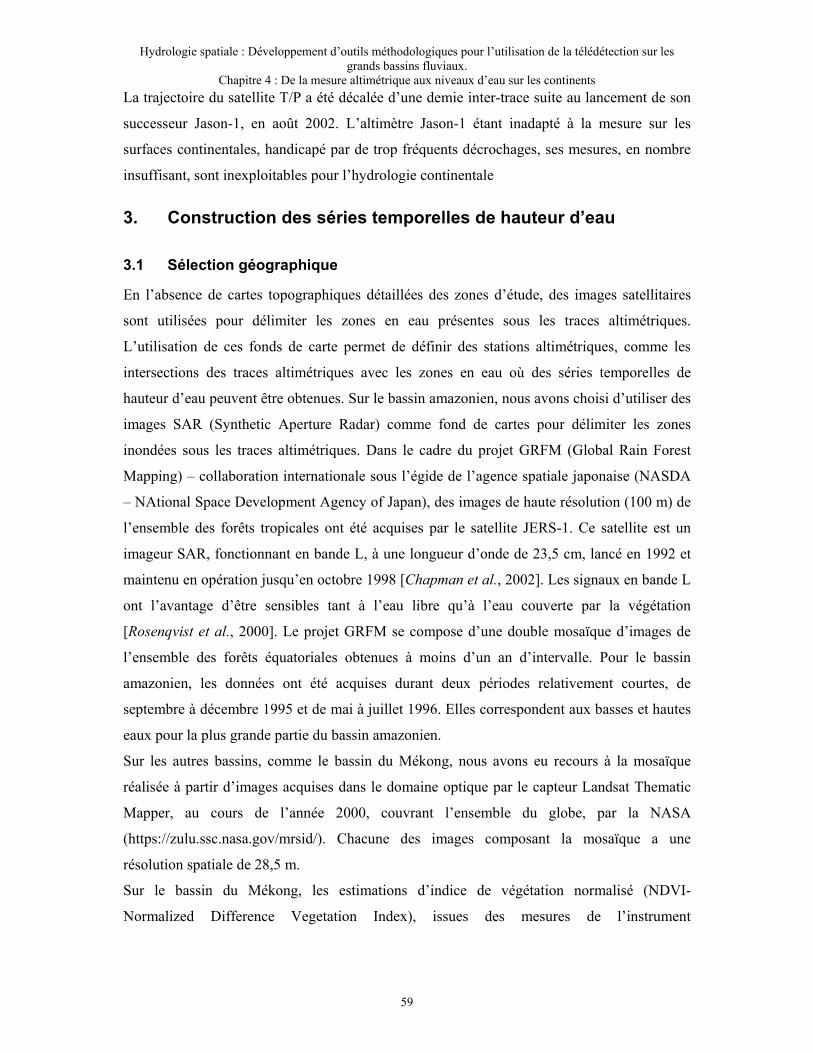
Hydrologie spatiale : Développement d’outils méthodologiques pour l’utilisation de la télédétection sur les grands bassins fluviaux.
Chapitre 4 : De la mesure altimétrique aux niveaux d’eau sur les continents
59
La trajectoire du satellite T/P a été décalée d’une demie inter-trace suite au lancement de son
successeur Jason-1, en août 2002. L’altimètre Jason-1 étant inadapté à la mesure sur les
surfaces continentales, handicapé par de trop fréquents décrochages, ses mesures, en nombre
insuffisant, sont inexploitables pour l’hydrologie continentale
3. Construction des séries temporelles de hauteur d’eau
3.1 Sélection géographique
En l’absence de cartes topographiques détaillées des zones d’étude, des images satellitaires
sont utilisées pour délimiter les zones en eau présentes sous les traces altimétriques.
L’utilisation de ces fonds de carte permet de définir des stations altimétriques, comme les
intersections des traces altimétriques avec les zones en eau où des séries temporelles de
hauteur d’eau peuvent être obtenues. Sur le bassin amazonien, nous avons choisi d’utiliser des
images SAR (Synthetic Aperture Radar) comme fond de cartes pour délimiter les zones
inondées sous les traces altimétriques. Dans le cadre du projet GRFM (Global Rain Forest
Mapping) – collaboration internationale sous l’égide de l’agence spatiale japonaise (NASDA
– NAtional Space Development Agency of Japan), des images de haute résolution (100 m) de
l’ensemble des forêts tropicales ont été acquises par le satellite JERS-1. Ce satellite est un
imageur SAR, fonctionnant en bande L, à une longueur d’onde de 23,5 cm, lancé en 1992 et
maintenu en opération jusqu’en octobre 1998 [Chapman et al., 2002]. Les signaux en bande L
ont l’avantage d’être sensibles tant à l’eau libre qu’à l’eau couverte par la végétation
[Rosenqvist et al., 2000]. Le projet GRFM se compose d’une double mosaïque d’images de
l’ensemble des forêts équatoriales obtenues à moins d’un an d’intervalle. Pour le bassin
amazonien, les données ont été acquises durant deux périodes relativement courtes, de
septembre à décembre 1995 et de mai à juillet 1996. Elles correspondent aux basses et hautes
eaux pour la plus grande partie du bassin amazonien.
Sur les autres bassins, comme le bassin du Mékong, nous avons eu recours à la mosaïque
réalisée à partir d’images acquises dans le domaine optique par le capteur Landsat Thematic
Mapper, au cours de l’année 2000, couvrant l’ensemble du globe, par la NASA
(https://zulu.ssc.nasa.gov/mrsid/). Chacune des images composant la mosaïque a une
résolution spatiale de 28,5 m.
Sur le bassin du Mékong, les estimations d’indice de végétation normalisé (NDVI-
Normalized Difference Vegetation Index), issues des mesures de l’instrument

Hydrologie spatiale : Développement d’outils méthodologiques pour l’utilisation de la télédétection sur les grands bassins fluviaux.
Chapitre 4 : De la mesure altimétrique aux niveaux d’eau sur les continents
60
VEGETATION, à bord du satellite SPOT-4, ont également été utilisées. Ces images, de
répétitivité temporelle égale à 10 jours, ont une résolution spatiale kilométrique.
Ces images satellitaires sont suffisamment précises pour permettre l’identification du cours
des fleuves étudiées et de leurs affluents. L’identification des zones inondées présentes dans
les bassins versants est, en revanche, moins aisée. Elle nécessite de recourir à des techniques
sur lesquelles nous reviendrons au chapitre 5.
3.2 Sélection des mesures valides
A chaque intersection entre une trace satellite et le fleuve (ou une zone inondée), une station
altimétrique peut-être définie. Les hauteurs d’eau sont calculées, à partir des mesures
altimétriques à haute-fréquence (10 Hz pour T/P et 20 Hz pour ERS-1&2 et ENVISAT), au
moyen de l’équation (Eq. 2-8). Si l’un des paramètres intervenant dans cette équation a une
valeur aberrante, au vu des critères définis par les agences spatiales, la mesure est éliminée.
La hauteur d’eau moyenne sur l’ensemble des cycles altimétriques est ensuite estimée, ainsi
que l’écart-type associé. L’ensemble des points de mesure s’écartant de la valeur moyenne de
plus trois fois la valeur de la dispersion (filtrage à « 3 sigmas » correspondant à un intervalle
de confiance de 99,7%) sont éliminés.
3.3 Séries temporelles de hauteur d’eau
Les séries temporelles de hauteur d’eau sont obtenues en calculant la médiane, sur la durée
d’un cycle, des hauteurs d’eau dérivées des mesures altimétriques contenues dans la fenêtre
rectangulaire correspondant à la station virtuelle considérée (Figure 4-1). A chaque point de la
série temporelle est associée une dispersion caractérisant la qualité des résultats ainsi obtenus.
En norme L1, la dispersion est fournie par l’estimateur :
∑= −−= N
i
medi hhN
hEAM11
1)( (Eq. 4-1)
où EAM(h) est l’écart absolu médian des observations, N le nombre d’observations, hi la ième
observation et hmed la médiane des observations.

Hydrologie spatiale : Développement d’outils méthodologiques pour l’utilisation de la télédétection sur les grands bassins fluviaux.
Chapitre 4 : De la mesure altimétrique aux niveaux d’eau sur les continents
61
Les niveaux d’eau sont exprimés par rapport au géoïde EIGEN-GRACE02C, développé
jusqu’à l’harmonique 150, obtenu à partir des mesures gravimétriques acquises au cours de la
première année de fonctionnement de la mission spatiale GRACE [Reigber et al., 2005], sur
laquelle nous reviendrons dans le chapitre 7. Les Figures 4-2, 4-3 et 4-4 présentent des
exemples de séries temporelles de hauteur obtenues à partir des mesures altimétriques
d’ENVISAT sur le Rio Negro et ses affluents (bassin amazonien). Les fonds de carte utilisés
sont des images JERS-1, les rectangles verts symbolisent les stations virtuelles, les traces
d’ENVISAT sont représentées en bleu, et les traces T/P en rouge.
Figure 4-1: Exemple de station virtuelle sur le Gange. Le carré blanc délimite la fenêtre de sélection des données, le trait rouge
représente la trace moyenne de T/P. Les losanges correspondent aux mesures à 10 Hz sélectionnées pour les cycles 214 (rouge),
215 (vert) et bleu (216) (Document GOHS, LEGOS, Toulouse).
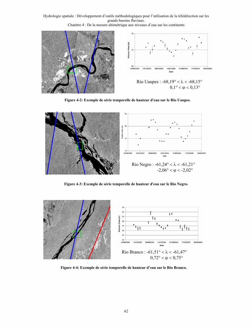
Hydrologie spatiale : Développement d’outils méthodologiques pour l’utilisation de la télédétection sur les grands bassins fluviaux.
Chapitre 4 : De la mesure altimétrique aux niveaux d’eau sur les continents
62
Rio Uaupes : -68,19° < λ < -68,15° 0,1° < ϕ < 0,13°
Figure 4-2: Exemple de série temporelle de hauteur d'eau sur le Rio Uaupes.
Rio Negro : -61,24° < λ < -61,21° -2,06° < ϕ < -2,02°
Figure 4-3: Exemple de série temporelle de hauteur d'eau sur le Rio Negro.
Rio Branco : -61,51° < λ < -61,47° 0,72° < ϕ < 0,75°
Figure 4-4: Exemple de série temporelle de hauteur d’eau sur le Rio Branco.

Hydrologie spatiale : Développement d’outils méthodologiques pour l’utilisation de la télédétection sur les grands bassins fluviaux.
Chapitre 4 : De la mesure altimétrique aux niveaux d’eau sur les continents
63
4. Application à la validation des hauteurs d’eau déduites des
mesures d’ENVISAT
4.1 Choix de la zone d’étude
Pour estimer la qualité des séries temporelles calculées au niveau des stations virtuelles, la
méthode la plus fiable consiste à comparer les mesures altimétriques avec les observations in-
situ les plus proches dans l’espace et le temps. De nombreuses études ayant utilisé l’altimétrie
satellitaire pour le suivi des niveaux d’eau dans les grands bassins fluviaux, ont eu pour cadre
le bassin amazonien [Birkett, 1998 ; de Oliveira Campos et al., 2001 ; Birkett et al., 2002].
Ces études ont proposé des estimations de la précision des mesures de T/P par comparaison
avec des données in-situ. Avec une méthodologie comparable, nous présentons des résultats
de validation des mesures de l’altimètre d’ENVISAT.
Pour cette étude, nous avons sélectionné, sur le bassin amazonien, 8 stations limnimétriques
gérées soit par l’agence de l’eau brésilienne (Agencia Nacional de Aguas –ANA-
http://www.ana.gov.br), soit par le projet HYBAM (Hydrologie du Bassin AMazonien –
http://www.mpl.ird.fr/hybam) respectant les critères suivants :
- la station est nivelée par GPS,
- ses niveaux d’eau journaliers sont disponibles pour la période 2002-2004,
- elle est à une distance inférieure à 50 km d’une trace ENVISAT.
Leur situation géographique, ainsi que la valeur du nivellement GPS associé, est présenté dans
le Tableau 4-2.
Station Basin Long (°) Lat (°) Stage-0 altitude (m wrt GRACE)
Tabatinga Solimões-Amazon
-69.933 -4.25 55.98
Manacapuru Solimões-Amazon
-60.609 -3.308 3.87
Obidos Solimões-Amazon
-55.511 -1.947 2.41
Curuai Solimões-Amazon
-55.476 -2.267 -0.77
Tabatinga do Salé
Solimões-Amazon
-55.78 -2.25 4.55
Curicuriari Negro -66.812 -0.192 32.46 Tapuracuara Negro -65.015 -0.42 25.45 Manaus Negro -60.035 -3.149 -7.5
Tableau 4-2: Situation géographique des stations in-situ.

Hydrologie spatiale : Développement d’outils méthodologiques pour l’utilisation de la télédétection sur les grands bassins fluviaux.
Chapitre 4 : De la mesure altimétrique aux niveaux d’eau sur les continents
64
4.2 Comparaison avec les mesures in-situ
Les séries temporelles de hauteur d’eau, déduites du retraitement des échos radar par quatre
algorithmes spécialisés et obtenues avec la méthode décrite au paragraphe précédent, ont été
comparées avec les observations in-situ. L’algorithme « Ice-1 » fournit entre 8 et 15% de plus
de mesures utilisables que les autres algorithmes. La dispersion, associée à la hauteur d’eau
médiane calculée à chaque cycle, est plus faible avec « Ice-1 » qu’avec les autres algorithmes.
Elle est généralement inférieure à 20 cm pendant l’étiage et à 10 cm pendant la crue (Figure
4-5 à la station de Tabatinga do Salé, pouvant même être égale à 5 cm lorsque la rivière est
suffisamment large (voir l’exemple de Manaus sur la Figure 4-6).
Figure 4-5: Séries temporelles de niveau d'eau estimée ENVISAT (points gris) et enregistrée à la station
de Tabatinga do Salé (trait gris).

Hydrologie spatiale : Développement d’outils méthodologiques pour l’utilisation de la télédétection sur les grands bassins fluviaux.
Chapitre 4 : De la mesure altimétrique aux niveaux d’eau sur les continents
65
Les écarts quadratiques moyens entre les niveaux d’eau altimétriques et in-situ sont présentés
dans le Tableau 1-2.
Reference ENVISAT
track
RMS Error (m)
Station Position
(km)
Ocean Ice-1 Ice-2 Sea Ice
Tabatinga 20 lower 0.27 0.40 0.32 1.37 Manacapuru 43.5 upper 0.27 0.20 0.86 0.69 Manacapuru 43.5 lower 0.31 0.27 0.29 0.21 Obidos 5.25 lower 0.26 0.26 0.58 0.4 Tabatinga do Salé
Lake 1 0.85 0.36 0.90 1.08
Tabatinga do Salé
Lake 2 1.40 0.25 1.10 3.24
Curuai Lake 3 0.55 0.53 1.35 0.99 Curicuriari 29 upper 0.12 0.07 0.10 0.13 Tapuruquara 15.5 upper 0.50 0.35 0.42 0.33 Tapuruquara 47.5 lower 0.42 0.12 0.23 0.14 Manaus 29 upper 0.31 0.11 0.56 0.32
Tableau 4-3: Ecarts quadratiques moyens entre les enregistrements
des stations hydrographiques et les mesures d'ENVISAT.
Figure 4-6 : Séries temporelles de niveau d'eau estimée ENVISAT (points gris) et enregistrée à la station
de Manaus (trait gris).

Hydrologie spatiale : Développement d’outils méthodologiques pour l’utilisation de la télédétection sur les grands bassins fluviaux.
Chapitre 4 : De la mesure altimétrique aux niveaux d’eau sur les continents
66
Dans la grande majorité des cas, les écarts quadratiques moyens entre niveaux d’eau
altimétriques et in-situ sont plus faibles avec l’algorithme « Ice-1 ». De meilleurs résultats
sont obtenus sur les fleuves que sur les plaines d’inondation (stations de Curuaí et de
Tabatinga do Salé). Dans la suite des travaux présentés, les données altimétriques ENVISAT
utilisées seront celles retraitées avec l’algorithme « Ice-1 ».
4.3 L’exemple de la várzea de Curuaí
La várzea de Curuaí, située au sud d’Óbidos, peut-être considérée représentative d’un grand
nombre de plaines d’inondation disséminées le long du cours principal de l’Amazone.
S’étendant sur une longueur de plus de 100 km sur la rive droite de l’Amazone, elle est
composée d’une vingtaine de lacs interconnectés et communiquant avec le fleuve par des
canaux permanents ou temporaires (Figure 4-7). Son fonctionnement hydrologique est suivi
dans le cadre du projet HYBAM, dont les membres ont réalisé 17 campagnes de mesures sur
ce site.
Une des principales interrogations concerne l’apport des données d’altimétrie satellitaire pour
l’étude du fonctionnement hydrologique de la várzea de Curuaí, principalement en terme de
précision. Des séries temporelles de hauteur d’eau ont pu être construites sur trois lacs de la
várzea de Curuaí. Ces séries temporelles, présentées sur la Figure 4-8, ont été comparées avec
les enregistrements des stations hydrographiques de Tabatinga do Salé pour les lacs 1 et 2 et
Figure 4-7: Représentation des traces altimétriques ENVISAT (vert), T/P (bleu) et
ICESat (rouge). Le fond de carte provient du modèle numérique SRTM (Rabus et al.,
2003).
Lac 1
Lac 2
Lac 3

Hydrologie spatiale : Développement d’outils méthodologiques pour l’utilisation de la télédétection sur les grands bassins fluviaux.
Chapitre 4 : De la mesure altimétrique aux niveaux d’eau sur les continents
67
Curuaí pour le lac 3. La précision des résultats obtenus a été examinée au moyen des cinq
estimateurs suivants:
- la dispersion des données altimétriques,
- le bais entre les mesures altimétriques et in-situ,
- l’écart quadratique moyen entre les mesures altimétriques et in-situ,
- le coefficient de corrélation entre les mesures altimétriques et in-situ,
- l’équation de régression linéaire.
Les statistiques obtenues sont présentées dans le Tableau 4-4 et les graphiques correspondants
sur la Figure 4-9.
Figure 4-8: Séries temporelles de hauteur d'eau sur les 3 lacs de la
varzea de Curuai. Comparaisons avec les observations faites à
Tabatinga do Salé (lacs 1 et 2) et Curuai (lac 3).

Hydrologie spatiale : Développement d’outils méthodologiques pour l’utilisation de la télédétection sur les grands bassins fluviaux.
Chapitre 4 : De la mesure altimétrique aux niveaux d’eau sur les continents
68
La dispersion des niveaux d’eau obtenus par altimétrie est faible (<30 cm) sauf pour le 3ème,
où elle est égale à 58 cm. Cette valeur relativement élevée résulte de la nature de l’intersection
de la trace satellitaire avec le lac : sa largeur n’est que de quelques centaines de mètres entre
des bancs de sable recouverts par de la végétation. La qualité de la mesure radar est affectée
par les réflexions parasites provenant des différents types de surface (eau, sable, végétation)
contenues dans la tâche au sol de l’altimètre.
σ (m) Biais (m) RMS (m) Coefficient
de corrélation
Régression linéaire : y=ax+b
σa
σb (m)
Lac 1 0,22 0,71 0,36 0,98 y=0,94x+1,1 0,24 0,08 Lac 2 0,30 0,24 0,25 0,99 y=0,89x+0,5 0,19 0,06 Lac 3 0.,58 -0,32 0,53 0,96 y=1,01x-0,43 0,52 0,17
Tableau 4-4: Comparaison des niveaux d’eau aux stations hydrographiques et déduits des mesures
d’ENVISAT sur la várzea de Curuai.
Les valeurs de l’écart quadratique moyen entre données d’ENVISAT et observations in-situ
sont assez faibles, les valeurs des coefficients de corrélation proches de 1, de même que les
coefficients directeurs des droites de régression. Ces statistiques témoignent d’un bon accord
entre données altimétriques et in-situ. Les formes d’onde altimétriques d’ENVISAT, retraitées
par l’algorithme « Ice-1 », fournissent des variations de niveau d’eau de qualité pour les
études hydrologiques.
Figure 4-9 : Comparaison des niveaux d'eau altimétriques et de stations hydrographiques sur la várzea de Curuai.
Lac 1 Lac 2
Lac 3

Hydrologie spatiale : Développement d’outils méthodologiques pour l’utilisation de la télédétection sur les grands bassins fluviaux.
Chapitre 4 : De la mesure altimétrique aux niveaux d’eau sur les continents
69
Néanmoins, les biais entre mesures altimétriques et relevés effectués aux stations
limnimétriques s’échelonnent de –32 à 71 cm. Il est assez difficilement envisageable que ces
biais soient dus à une erreur dans le nivellement GPS des stations.
Ces différences pourraient provenir des ondulations du géoïde aux courtes longueurs d’onde,
non prises en compte par le modèle EIGEN-GRACE02C. Des erreurs dans les corrections
instrumentales, géophysiques ou de propagation pourraient expliquer ces biais. Il est plus
vraisemblable de penser que ces différences sont dues à un manque de précision des données
altimétriques ou à des causes hydrologiques. En effet, tous les lacs de la várzea de Curuaí
n’ont pas nécessairement le même niveau et ce niveau n’est pas nécessairement constant sur
toute la surface du lac. Des pentes de 2 cm/km ont été trouvées en utilisant les mesures de
l’altimètre laser ICESat (Stéphane Calmant, communication personnelle). Seuls des études
plus approfondies, nécessitant de nouvelles campagnes de mesures, permettront de déterminer
les causes des différences observées.
L’ensemble des résultats obtenus dans le cadre de la validation des données ENVISAT sur les
eaux continentales est présenté dans l’Annexe 1.
5. Conclusion
Une méthodologie fiable permettant la création de stations virtuelles où des variations de
niveau d’eau peuvent être estimées a été définie. Les résultats de validation mettent en
évidence la bonne qualité des mesures altimétriques d’ENVISAT (écarts quadratiques moyens
inférieurs à 30 cm). Des méthodes similaires ont permis d’évaluer la précision des données
T/P à des valeurs comprises entre 30 et 50 cm [Birkett , 1998 ; de Oliveira Campos, 2001 ;
Birkett et al., 2002]. Les données ERS-2 ont pour l’instant été très peu utilisées pour l’étude
des eaux continentales. Des précisions similaires à celles de T/P ont été obtenues sur le Rio
Tapajos (bassin amazonien, cf. Annexe 1) et sur le Mékong (Figure 4-10 et cf. Annexe 2).
Des études permettant d’évaluer les biais entre les différents capteurs sont actuellement en
cours.

Hydrologie spatiale : Développement d’outils méthodologiques pour l’utilisation de la télédétection sur les grands bassins fluviaux.
Chapitre 4 : De la mesure altimétrique aux niveaux d’eau sur les continents
70
Figure 4-10 : Comparaison T/P - ERS-2 dans le bassin du Mékong. Séries temporelles de hauteur
d’eau : en bleu T/P, en noir ERS-2 et en rouge la différence.

Hydrologie spatiale : Développement d’outils méthodologiques pour l’utilisation de la télédétection sur les
grands bassins fluviaux
Chapitre 5 : Estimation des profils hydrologiques des fleuves au moyen de l’altimétrie satellitaire
71
Chapitre 5 : Estimation des profils hydrologiques des fleuves au moyen de l’altimétrie satellitaire
Chapitre 5 : Estimation des profils hydrologiques des fleuves au
moyen de l’altimétrie satellitaire ........................................................71
1. Introduction .................................................................................................................. 72
2. Intérêt de l’estimation des profils hydrologiques ......................................................... 72
3. Profil hydrologique du Rio Negro et de ses affluents .................................................. 73
3.1 Données utilisées.................................................................................................. 73
3.2 Profils longitudinaux ............................................................................................ 74
4. Comparaison avec d’autres sources de données .......................................................... 77
4.1 Comparaison avec des mesures GPS ................................................................... 77
4.2 Comparaison avec les sorties du modèle Muskingum-Cunge ............................. 78
5. Conclusion.................................................................................................................... 79

Hydrologie spatiale : Développement d’outils méthodologiques pour l’utilisation de la télédétection sur les
grands bassins fluviaux
Chapitre 5 : Estimation des profils hydrologiques des fleuves au moyen de l’altimétrie satellitaire
72
1. Introduction
Etant donné la couverture spatiale des missions altimétriques actuelles, il existe un grand
nombre d’intersection des traces altimétriques avec les réseaux fluviaux. Des stations
virtuelles peuvent ainsi être définies, comme nous l’avons vu plus haut. A l’échelle des grands
bassins fluviaux, des produits dérivés de l’altimétrie satellitaire à vocation hydrologique ont
ainsi pu être développés, comme le profil de hauteur d’eau le long des fleuves ou les
variations de volume d’eau de surface (cf. chapitre 6).
La zone retenue pour l’estimation de profils hydrologiques par altimétrie satellitaire est le
bassin du Rio Negro. Ce bassin présente en effet l’avantage d’être une zone d’étude prioritaire
pour le projet HYBAM et par conséquent d’avoir fait l’objet de nombreuses campagnes de
mesures. Les dernières en date se sont déroulées, en novembre 2003, sur le Rio Branco et en
mai 2005, sur la partie centrale du Rio Negro.
En outre, des données journalières de hauteur d’eau et de débit provenant des stations
limnimétriques de l’agence de l’eau brésilienne (ANA) et validées par le projet HYBAM sont
également disponibles, permettant de valider les résultats obtenus.
2. Intérêt de l’estimation des profils hydrologiques
Les profils hydrologiques des fleuves sont concaves, et leur concavité traduit des effets
tectoniques, sédimentaires et climatiques. Les changements climatiques peuvent avoir pour
conséquence d’accroître l’érosion du lit de la rivière, de changer les apports sédimentaires, et
donc d’entraîner des modifications des profils longitudinaux des fleuves [Panagoulia et
Dimou, 1997 ; Zaprowski et al., 2005].
La connaissance du profil hydrologique d’un fleuve, préalable au calcul de la pente du fleuve,
est un paramètre important pour les études hydrologiques régionales ou locales. Son intérêt
géomorphologique est indéniable : la pente est utilisée dans l’estimation de l’intensité du flot
(stream power) d’un cours d’eau, l’un des facteurs primordiaux intervenant dans la formation
des chenaux [Alabyan et Chalov, 1998 ; Eaton et al., 2004 ; Ferguson, 2005]. Elle influe
également sur le transport des sédiments et la propagation du pic de crue [Birkett et al., 2002].
Elle donne accès à l’estimation des débits au moyen de l’équation de Manning :
2/13/5 SWZnkD= (Eq. 5-1)
où k est un facteur de conversion (valant 1 m1/3
/s), n le coefficient de Manning, lié à la
rugosité du lit du fleuve, W, la largeur du fleuve, Z sa profondeur, et S sa pente.

Hydrologie spatiale : Développement d’outils méthodologiques pour l’utilisation de la télédétection sur les
grands bassins fluviaux
Chapitre 5 : Estimation des profils hydrologiques des fleuves au moyen de l’altimétrie satellitaire
73
Cette méthode a été récemment employée par Le Favour et Alsdorf [2005] pour estimer des
débits sur le bassin amazonien à partir des pentes calculées au moyen du Modèle Numérique
de Terrain (MNT) SRTM (Shuttle Radar Topography Mission) [Rabus et al., 2003].
Ce paramètre est cependant difficile à mesurer sur le terrain. L’avantage de l’utilisation de la
télédétection, par rapport aux méthodes classiques, réside dans sa capacité à fournir des
informations à l’échelle des bassins versants, et en particulier sur des zones difficiles d’accès
[Bjerklie et al., 2005].
3. Profil hydrologique du Rio Negro et de ses affluents
3.1 Données utilisées
Pour cette étude, nous avons utilisé les mesures :
- à 10 Hz de Topex/Poseidon entre les cycles 3 et 362, couvrant la période allant
d’octobre 1992 à août 2002 (ancienne orbite),
- à 20 Hz acquises par l’altimètre RA-2 du satellite ENVISAT entre les cycles 10 et 37
couvrant la période allant d’octobre 2002 à juin 2005 et retraitées avec l’algorithme
Ice-1 [Bamber, 1994].
Suivant la méthodologie présentée au chapitre 4, des stations virtuelles ont été définies aux
intersections des traces altimétriques avec le Rio Negro et ses principaux affluents, les Rio
Negro et Uaupes (Figure 5-1).
Le Tableau 5-1 présente le nombre de stations altimétriques présentes sur chaque fleuve par
capteur.
Rio Negro Uaupes Rio Branco
T/P 14 3 3
ENVISAT 29 13 6
Tableau 5-1: Nombre de stations virtuelles utilisées pour l'estimation des profils.
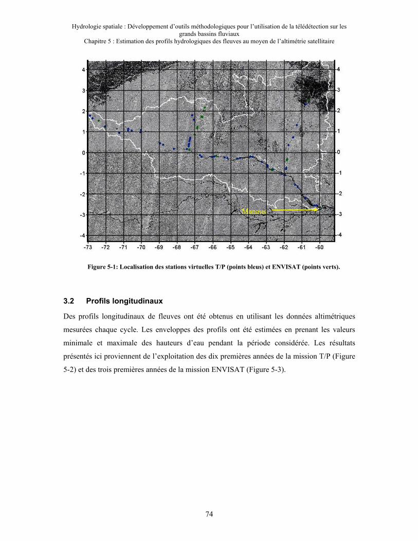
Hydrologie spatiale : Développement d’outils méthodologiques pour l’utilisation de la télédétection sur les
grands bassins fluviaux
Chapitre 5 : Estimation des profils hydrologiques des fleuves au moyen de l’altimétrie satellitaire
74
3.2 Profils longitudinaux
Des profils longitudinaux de fleuves ont été obtenus en utilisant les données altimétriques
mesurées chaque cycle. Les enveloppes des profils ont été estimées en prenant les valeurs
minimale et maximale des hauteurs d’eau pendant la période considérée. Les résultats
présentés ici proviennent de l’exploitation des dix premières années de la mission T/P (Figure
5-2) et des trois premières années de la mission ENVISAT (Figure 5-3).
Figure 5-1: Localisation des stations virtuelles T/P (points bleus) et ENVISAT (points verts).
Manaus

Hydrologie spatiale : Développement d’outils méthodologiques pour l’utilisation de la télédétection sur les
grands bassins fluviaux
Chapitre 5 : Estimation des profils hydrologiques des fleuves au moyen de l’altimétrie satellitaire
75
Figure 5-2: Profils longitudinaux des Rio Uaupes (haut), Negro (milieu) et
Branco (bas) d'après T/P, calculées au date de la mosaïque JERS-1 et aux
minima de 1995 et maxima de 1996.

Hydrologie spatiale : Développement d’outils méthodologiques pour l’utilisation de la télédétection sur les
grands bassins fluviaux
Chapitre 5 : Estimation des profils hydrologiques des fleuves au moyen de l’altimétrie satellitaire
76
Figure 5-3: Profils longitudinaux des Rio Uaupes (haut), Negro (milieu) et Branco (bas),
estimés à partir des mesures altimétriques d'ENVISAT en 2003 et 2004.

Hydrologie spatiale : Développement d’outils méthodologiques pour l’utilisation de la télédétection sur les
grands bassins fluviaux
Chapitre 5 : Estimation des profils hydrologiques des fleuves au moyen de l’altimétrie satellitaire
77
De grandes similitudes sont observées entre les profils estimés en basses et hautes eaux par
chacun des différents capteurs. Les différences entre basses et hautes eaux reflètent les
caractéristiques hydrologiques de la zone d’étude : une amplitude annuelle de 10 mètres ou
plus, est bien présente en aval du Rio Negro, à proximité de Manaus.
Il est toutefois difficile de comparer de manière précise les profils restitués par T/P et par
ENVISAT, même si des analogies existent, car les périodes considérées et l’échantillonnage
temporel sont différents. Des comparaisons avec d’autres sources d’information sont
nécessaires pour la validation des profils calculés.
4. Comparaison avec d’autres sources de données
4.1 Comparaison avec des mesures GPS
En novembre 2003, une campagne de mesures, à laquelle j’ai participé, a été réalisée sur le
Rio Branco par l’équipe HYBAM du LMTG, dans le but d’améliorer la connaissance des
processus de transports et de remaniement sédimentaire ayant lieu dans la plaine
amazonienne, sous l’effet de la variabilité climatique (cf. le rapport de campagne figurant
dans l’Annexe 1). Un des objectifs de cette mission était de proposer une méthodologie de
calibration et de validation des mesures altimétriques par des données in-situ. Pour ce faire,
un profil de hauteur du Rio Branco a été réalisé à l’aide des mesures GPS acquises entre le 12
et le 16 novembre. Ces dates correspondent au cycle 21 et 22 d’ENVISAT avec lesquels des
comparaisons ont été effectuées. La Figure 5-4 présente les profils obtenus pour les cycles 21,
dont les dates varient du 26/10/2003 au 14/11/2003, 22 (du 30/11/2003 au 11/12 :2003) et à
partir des moyennes des mesures GPS au niveau des stations virtuelles. Les hauteurs d’eau
estimées par altimétrie sont proches de celles mesurées par GPS avec des écarts variant de 2
cm à 1,15 m. Des différences peuvent pourtant être observées sur la courbure des différents
profils. Les hauteurs GPS sont plus élevées que les hauteurs altimétriques près de
l’embouchure avec le Negro et aux distances comprises entre 550 et 700 km de Manaus. Ces
différences, vraisemblablement à la propagation d’un pic de crue, causé par des précipitations,
peuvent s’expliquer du fait du décalage temporel entre mesures GPS et observations
altimétriques.

Hydrologie spatiale : Développement d’outils méthodologiques pour l’utilisation de la télédétection sur les
grands bassins fluviaux
Chapitre 5 : Estimation des profils hydrologiques des fleuves au moyen de l’altimétrie satellitaire
78
4.2 Comparaison avec les sorties du modèle Muskingum-Cunge
Des études de propagation des débits ont été entreprises au LMTG, par Juan Gabriel León, au
moyen du modèle de routage Muskingum-Cunge, sur la partie amont du Rio Negro. Cette
méthode permet d’estimer des débits le long du cours principal, moyennant la connaissance
des débits en amont et des apports latéraux des affluents (cf. Annexe 3). Il est ainsi possible
de retrouver le lit du fleuve en inversant l’équation :
bhHaD )( −= (Eq. 5-2)
où D est le débit, (H-h) le niveau d’eau par rapport au lit du fleuve, a et b des paramètres
caractéristiques de la section de fleuve considéré.
La résolution de ce problème inverse où D (débit simulé) et H (niveau d’eau estimé par
altimétrie) sont connus donne accès au profil du lit du fleuve h.
Le résultat pour le cours supérieur du Rio Negro est présenté sur la Figure 5-5.
Figure 5-4: Profil du Rio Branco estimé par altimétrie (ENVISAT) et GPS.

Hydrologie spatiale : Développement d’outils méthodologiques pour l’utilisation de la télédétection sur les
grands bassins fluviaux
Chapitre 5 : Estimation des profils hydrologiques des fleuves au moyen de l’altimétrie satellitaire
79
Figure 5-5: Estimation des profils hydrologiques du lit et des niveaux basses et hautes eaux du cours
supérieur du Rio Negro.
Un très bon accord est observé entre les différents profils calculés. Les déformations des
surfaces libres observées par altimétrie satellitaire sont reproduites par le modèle au niveau du
lit du fleuve.
5. Conclusion
Les niveaux d’eau dérivés du traitement des mesures altimétriques ont l’avantage,
contrairement à ceux mesurés par les réseaux limnimétriques classiques, d’être donnés par
rapport à une référence unique, ellipsoïdale ou géoïdale. Dans ce dernier cas, ils permettent
l’estimation des profils longitidunaux des fleuves et de leur pente.
Néanmoins, ils ont l’inconvénient de ne pas fournir une mesure journalière de hauteur d’eau,
rendant difficile l’estimation des profils et des pentes. Ceci implique le recalage des mesures à
une date commune. Un travail de ce type est actuellement en cours dans le cadre d’une
collaboration entre les équipes HYBAM du LMTG et GOHS du LEGOS. Il porte sur la
comparaison des pentes estimées par différentes techniques :
- altimétrie radar (T/P et ENVISAT),
- altimétrie laser (ICESat)
- modélisation hydrologique (méthode Muskingum-Cunge)
- campagnes de mesures GPS,

Hydrologie spatiale : Développement d’outils méthodologiques pour l’utilisation de la télédétection sur les
grands bassins fluviaux
Chapitre 5 : Estimation des profils hydrologiques des fleuves au moyen de l’altimétrie satellitaire
80
- stations hydrographiques nivelées du bassin du Rio Negro.
La connaissance des pentes des fleuves sur l’ensemble d’un bassin permettra de niveler
l’ensemble des stations limnimétriques. Nous disposerons ainsi d’un réseau de mesures dense,
combinant données altimétriques et relevés in-situ, permettant de suivre différents paramètres
hydrologiques, comme la propagation des pics de crue.

Hydrologie spatiale : Développement d’outils méthodologiques pour l’utilisation de la télédétection sur les grands bassins fluviaux
Chapitre 6 : Variations de volume d’eau de surface dans les grands bassins fluviaux
81
Chapitre 6 : Variations de volume d’eau de surface dans les grands bassins fluviaux – Etude de la synergie altimétrie satellitaire/imagerie spatiale
Chapitre 6 : Variations de volume d’eau de surface dans les grands bassins fluviaux – Etude de la synergie altimétrie satellitaire/imagerie spatiale................................................................................................81
1. Introduction .................................................................................................................. 82 2. Méthode d’estimation des variations de volume d’eau ................................................ 83
2.1 Le bassin du Rio Negro........................................................................................ 83 2.2 Identification des zones en eau............................................................................. 84 2.3 Les cartes de hauteur d’eau .................................................................................. 86 2.4 Estimation des variations de volume d’eau.......................................................... 87 2.5 Résultats ............................................................................................................... 87 2.6 Article “Floodplain water storage in the Negro River basin estimated from microwave remote sensing of inundation area and water levels “ ................................... 88
3. Variations inter-annuelles de volume d’eau de surface dans la partie avale du bassin du Mékong............................................................................................................................... 102
3.1 Caractéristiques hydrologiques de la zone étudiée ............................................ 102 3.2 Délimitation des zones inondées ........................................................................ 103 3.3 Cartes de hauteur d’eau ...................................................................................... 105 3.4 Estimation des variations de volume d’eau........................................................ 107 3.5 Résultats ............................................................................................................. 107 3.6 Article “Water volume change in the lower Mekong basin from satellite altimetry and other remote sensing data” ...................................................................................... 109
4. Conclusion.................................................................................................................. 139

Hydrologie spatiale : Développement d’outils méthodologiques pour l’utilisation de la télédétection sur les grands bassins fluviaux
Chapitre 6 : Variations de volume d’eau de surface dans les grands bassins fluviaux
82
1. Introduction
Les zones d’inondation, présentes le long des grands fleuves, jouent un rôle non négligeable
dans le cycle hydrologique des grands bassins fluviaux [Alsdorf et al., 2001; Richey et al.,
1989]. Le transport de l’eau et des sédiments est affecté par leur séjour dans les zones
d’inondation: l’eau est non seulement retardé dans son écoulement vers la mer et sujet à
l’évapotranspiration, mais aussi l’objet d’importants changements biogéochimiques liés à la
sédimentation, à la captation de nutriments par le biotope ou à la modification des conditions
d’oxydo-réduction [Hamilton et al., 2002].
La détermination des variations temporelles de volumes d’eau stockés dans les plaines
d’inondation des grands bassins fluviaux, est de grande importance dans les études
hydrologiques. Pour les zones inondées, de manière temporaire ou permanente et connectées
au cours principal du fleuve, déterminer leur variation de volume d’eau revient à estimer le
volume potentiellement stocké pendant la période de crue. Dans ce cas, les variations de
volume d’eau sont un paramètre capital pour la modélisation hydrodamique des flux d’eau des
fleuves et des capacités de transport. Pour les zones d’inondation non connectées au cours
principal, les variations de volume d’eau sont fonction du flux de base, des apports locaux et
de la pluie.
Ce paramètre est difficilement mesurable au moyen de techniques couramment utilisées en
hydrologie. Dans la première partie de ce chapitre, nous proposons une méthode combinant
altimétrie satellitaire et imagerie spatiale pour le déterminer. Cette étude a pour cadre le
bassin du Rio Negro, en Amazonie, et les données utilisées proviennent :
1) des mesures altimétriques de T/P et de niveaux d’eau enregistrés dans des stations
hydrographiques
2) d'une classification d’images SAR JERS-1.
Nous avons ainsi pu estimer les variations maximales de volume d’eau pour le cycle
d’hydrologique 1995-1996. Dans la seconde partie de ce chapitre, une étude reprenant la
même méthodologie a été menée dans le bassin du Mékong pour la période 1998-2003 au
moyen des images de SPOT/VGT et des mesures altimétriques d’ERS-2 et d’ENVISAT.
Le choix des données de télédétection utilisées a été dicté par les caractéristiques des régions
étudiées. Dans le bassin du Rio Negro, de nombreuses zones inondées sont recouvertes par de
la végétation plus ou moins dense. Il était, de ce fait, nécessaire d’utiliser des images

Hydrologie spatiale : Développement d’outils méthodologiques pour l’utilisation de la télédétection sur les grands bassins fluviaux
Chapitre 6 : Variations de volume d’eau de surface dans les grands bassins fluviaux
83
permettant d’avoir accès à l’information hydrologique en dépit du couvert végétal. Nous
avons donc eu recours à la double mosaïque d’images SAR acquises par JERS-1 en 1995 et
1996.
Le bassin du Mékong est principalement couvert par de la végétation rase et des cultures
totalement submergées par l’eau en période d’inondation. Nous avons préféré utiliser les
images multispectrales acquises par le capteur SPOT/VGT, qui présentent l’avantage d’avoir
une meilleure répétitivité temporelle.
2. Méthode d’estimation des variations de volume d’eau
2.1 Le bassin du Rio Negro
Le sous-bassin du Rio Negro ne représente que 12% de la surface totale du basin amazonien.
Affluent le plus important de l’Amazone, il est le 5ème fleuve au monde en terme de débit
[Meade et al., 1991 ; Molinier et al., 1996 ; 1997]. Ses eaux sont de couleur noire, en raison
d’une forte concentration en matière organique dissoute et d’une faible charge sédimentaire
[Sternberg, 1975 ; Mounier et al., 2002]. Sa confluence avec le fleuve Solimões donne
naissance à l’Amazone en aval de Manaus. Il s’étend sur une zone allant de 73,25° à 59,35°
de longitude Ouest et de 5,4° Nord à 3,35° de latitude Sud (Figure 6-1).
Il draine une vaste région de 700,000 km², s’étendant sur la Colombie (10%), le Venezuela
(6%), la Guyane (2%) et le Brésil (82%). L’extension considérable des zones inondées
provient, d’une part de la faible pente de la rivière et d’autre part, de l’importance des taux de
précipitation. Les taux de précipitation dans le sous-bassin varient tant dans l’espace que dans
le temps. Les taux de précipitation annuels moyens varient de plus de 50% dans le sous-bassin
du Rio Negro, de moins de 2000 mm/an (avec des valeurs minimales inférieures à 1700
mm/an enregistrées dans la partie nord du basin du Rio Branco) à 2250 voire 2500 mm/an
près de Manaus et jusqu’à 3000 mm/an au nord ouest [Liebmann et Marengo, 2001].
L’apparition de la saison des pluies diffère grandement le long d’un gradient nord-sud: elle
débute en décembre dans le sud et en mars ou avril dans le nord, tandis qu’elle se termine de
mai à octobre [Marengo et al., 2001].

Hydrologie spatiale : Développement d’outils méthodologiques pour l’utilisation de la télédétection sur les grands bassins fluviaux
Chapitre 6 : Variations de volume d’eau de surface dans les grands bassins fluviaux
84
2.2 Identification des zones en eau
De nombreuses études ont montré que les images SAR acquises dans le cadre du projet
GRFM (Global Rain Forest Mapping) pouvaient être utilisées pour identifier le type
d’occupation des sols, l’extension des zones de déforestation et celle des plaines d’inondation
[Saatchi et al., 2000; Siqueira et al., 2003; Hess et al., 2003].
Pour notre étude, une approche de classification originale a été développée par Jean-Michel
Martinez. Il s’agit d’une méthode non supervisée, dont les données en entrée, ne sont pas les
coefficients de rétrodiffusion associés à chaque pixel et mesurés aux deux dates, mais le
coefficient de rétrodiffusion moyen et le rapport des deux. Le coefficient de rétrodiffusion
moyen caractérise le type de végétation et le rapport des deux, une variation entre les deux
dates. Si une variation significative est observée, cela signifie que le pixel est passé d’un état
sec vers un état inondé et réciproquement. Les artefacts dus au relief, à la présence de zones
Figure 6-1: Le bassin du Rio Negro et couverture spatiale de T/P. Les stations altimétriques sont
représentées par un point noir dans un hexagone blanc, les stations hydrographiques par une croix dans
un cercle blanc. Les parties sombres de l’image correspondent aux zones en eau.

Hydrologie spatiale : Développement d’outils méthodologiques pour l’utilisation de la télédétection sur les grands bassins fluviaux
Chapitre 6 : Variations de volume d’eau de surface dans les grands bassins fluviaux
85
urbaines ont été pris en compte et éliminés. Cette méthode conduit à la définition des 8 classes
présentées sur la Figure 6-2 :
1) eaux libres
2) forêts temporairement inondées
3) forêts non inondées
4) sols nus (ou couverts de végétation basse) non inondés
5) prairies temporairement inondées
6) forêts toujours inondées
7) végétation basse temporairement inondée
8) végétation toujours inondée
Les résultats de la classification de la double mosaïque d’images SAR ont permis de
cartographier les zones inondées pendant l’étiage (zones d’inondation permanentes) et la crue
(combinaison de zones d’inondation permanentes et temporaires), au cours du cycle
hydrologique 1995-1996. Les classes 1) et 6) correspondent aux basses eaux, tandis que les
classes 1), 2), 5), 6), 7) et 8) caractérisent les hautes eaux (Figure 6-3).
Figure 6-2: Résultat de la classification des images JERS-1.

Hydrologie spatiale : Développement d’outils méthodologiques pour l’utilisation de la télédétection sur les grands bassins fluviaux
Chapitre 6 : Variations de volume d’eau de surface dans les grands bassins fluviaux
86
2.3 Les cartes de hauteur d’eau
88 stations virtuelles, où des séries temporelles de hauteur d’eau ont pu être construites
suivant la méthode présentée dans le chapitre 4, ont été définies dans le bassin du Rio Negro
(Figure 6-1). La valeur de hauteur d’eau correspondant à la date d’acquisition de l’image SAR
(information que l’on peut trouver sur le site http://trfic.jpl.nasa.gov/GRFM/jersframe.html), a
été interpolée à partir des valeurs espacées de 10 jours de la série temporelle T/P.
A ce jeu de données, viennent s’ajouter les relevés de 8 stations in-situ nivelées, gérées par
l’ANA, dont les données ont été validées par l’HYBAM.
Les cartes de niveau d’eau ont été calculées par un schéma d’interpolation linéaire prenant en
compte les 8 plus proches voisins (Figure 6-4). Leur résolution spatiale est de 0,002°, ce qui
représente environ 200 m à l’équateur, limite inférieure, au dessous de laquelle, il est
impossible de définir une station virtuelle.
Figure 6-3: Situation en période d'étiage (rouge) et de crue (rouge+gris).

Hydrologie spatiale : Développement d’outils méthodologiques pour l’utilisation de la télédétection sur les grands bassins fluviaux
Chapitre 6 : Variations de volume d’eau de surface dans les grands bassins fluviaux
87
2.4 Estimation des variations de volume d’eau
Le bassin du Rio Negro a été ensuite subdivisé en 11 sous-bassins hydrographiques
correspondant à ses affluents principaux. Pour chaque sous-bassin, les grilles de différence de
hauteur entre crue et étiage (obtenues comme la différence des deux grilles présentées sur la
Figure 5-4) ont été convertis au format 3D d’Arcview (Triangulated Irregulated Network ou
TIN). Une résolution verticale de 10 cm a été choisie, correspondant à la précision maximale
que l’on est en droit d’attendre pour les données de T/P [Birkett, 1998]. Ces représentations
3D du volume d’eau stocké pendant le cycle hydrologique de 1995-1996 permettent de
calculer les variations de volume d’eau entre crue et étiage dans le bassin du Rio Negro.
2.5 Résultats
Les résultats de la méthode de classification nous ont permis d’estimer la surface totale
inondée est de 35 944 km² durant les basses eaux et de 152 721 km² durant les hautes eaux.
Ces chiffres illustrent l’importance des plaines d’inondation dans le bassin du Rio Negro.
En règle générale, la surface inondée est beaucoup plus grande durant la crue. Des situations
très diverses sont observées suivant les sous-bassins considérés. Dans la partie est (amont du
Negro et Uaupes), qui comprend les sous-bassins de Cucui, Curicuriari, Sao Felipe et
Serrinha, environ 5% est inondé durant les basses eaux, et une surface 2 à 3 fois plus
importante durant les hautes eaux. La situation est très différente dans la partie nord (sous-
bassin de Caracarai) et en aval (sous-bassins de Foz do Branco, Únini, Jaú et l’aval du Rio
Negro): les zones en eau pendant la crue représentent entre 15 et 30% de la surface, ce qui
correspond à un accroissement d’un facteur supérieur à 4.
Figure 6-4: Cartes de hauteur d'eau pour les basses et les hautes eaux.

Hydrologie spatiale : Développement d’outils méthodologiques pour l’utilisation de la télédétection sur les grands bassins fluviaux
Chapitre 6 : Variations de volume d’eau de surface dans les grands bassins fluviaux
88
Les variations de volume d’eau caractérisent le volume d’eau stocké dans les zones
d’inondation. Ces variations sont plus importantes aux confluences entre le cours principal et
ses affluents (sous-bassins de Serrinha, Foz do Branco, Rio Branco et l’aval du Rio Negro).
Pendant la crue, le niveau d’eau des affluents (Uaupes, Branco et Negro en tant qu’affluent du
Rio Solimões), est contrôlé par le niveau du cours principal, provoquant d’importantes
inondations le long du cours principal (Figure 6-3). L’intensité de ce phénomène est moindre
pendant l’étiage. Cette caractéristique avait déjà été observée par Meade et al. [1991] sur
l’ensemble du bassin amazonien, et plus particulièrement dans le bassin du Rio Negro.
Nous avons ensuite comparé les variations de volume au volume s’écoulant de chaque sous-
bassin, quand des données de débit étaient disponibles. La surface inondée d’un bassin est
d’autant plus grande que le rapport entre volume stocké et volume écoulé est petit. Cette
relation n’est cependant pas proportionnelle, et en conséquence, on ne peut estimer la capacité
de stockage des zones inondées d’un bassin à partir de leur surface (Figure 6-5).
2.6 Article “Floodplain water storage in the Negro River basin estimated
from microwave remote sensing of inundation area and water levels “
Cette étude a fait l’objet d’un article publié par Remote Sensing of Environment.
Figure 6-5: Comparaison volume stocké (V) / volume écoulé (F).

Floodplain water storage in the Negro River basin estimated from microwave
remote sensing of inundation area and water levels
Frederic Frappart a,b,*, Frederique Seyler b, Jean-Michel Martinez c, Juan G. Leon b, Anny Cazenave a
a Laboratoire d’Etudes en Geophysique et Oceanographie Spatiales, UMR 5566 (CNES/CNRS/IRD/UPS), Observatoire Midi-Pyrenees,
18 Av. Edouard Belin 31401 Toulouse Cedex 9, Franceb Laboratoire des Mecanismes et Transferts en Geologie, UMR 5563 (CNRS/IRD/UPS), Observatoire Midi-Pyrenees,
14, Av. Edouard Belin, 31400 Toulouse, Francec Laboratoire des Mecanismes et Transferts en Geologie, UMR 5563 (CNRS/IRD/UPS), Maison de la Teledetection, 500, rue J-F Breton,
34093 Montpellier Cedex 5, France
Received 7 March 2005; received in revised form 13 July 2005; accepted 27 August 2005
Abstract
The objective of this study is to determine spatio-temporal variations of water volume over inundated areas located in large river basins using
combined observations from the Synthetic Aperture Radar (SAR) onboard the Japanese Earth Resources Satellite (JERS-1), the Topex/Poseidon
(T/P) altimetry satellite, and in-situ hydrographic stations. Ultimately, the goal is to quantify the role of floodplains for partitioning water and
sediment fluxes over the great fluvial basins of the world. SAR images are used to identify the type of surface (open water, inundated areas, forest)
and, hence, the areas covered with water. Both radar altimetry data and in-situ hydrographic measurements yield water level time series. The basin
of the Negro River, the tributary which carries the largest discharge to the Amazon River, was selected as a test site. By combining area estimates
derived from radar images classification with changes in water level, variations of water volume (focusing on a seasonal cycle) have been
obtained. The absence of relationship between water volume and inundated area, reflecting the diverse and widely dispersed floodplains of the
basin, is one of the main result of this study.
D 2005 Elsevier Inc. All rights reserved.
Keywords: Remote sensing; Hydrology; Altimetry; Water level and water volume variation
1. Introduction
Extensive floodplains along large South American rivers,
such as Amazon, Parana or Orinoco, have a significant role in
the hydrological cycle of fluvial basins. Transport of water and
sediments by rivers is substantially modified during residence
of river water in floodplains. During its stay in these inundation
areas, river water is not only delayed in its transit to sea and
affected by evapotranspiration, but it is also often subject to
large biogeochemical changes due to sedimentation, nutrient
uptake by the biota, and modifications of redox conditions
(Hamilton et al., 2002). The water storage in these wetlands
and its outflow represent a significant part of the water balance
in the basin (Alsdorf et al., 2001; Richey et al., 1989).
Determining the temporal variation of water volume stored
in the floodplains of great river basins is the subject of many
applications in hydrology. For the inundated areas permanently
or temporarily connected to main channels, the determination
of the water volume variation is equivalent to the estimation of
water volume potentially stored and/or released by the valley
reach during flood stages. The water volume variation in this
type of inundated areas is an important parameter for the
hydrodynamic modeling of the river flow and the determina-
tion of its transport capacity. For the inundated areas that never
connect to the main channel, the volume variation is essentially
a function of the base flow variation, the inputs from the local
basin and the rain. Some floodplains present both types of
flooding zones. Areas where the river water mixes with the
local water are called ‘‘perirheic zones’’ (Mertes, 1997). In all
cases, the inundation area is a buffer zone between the river
and the upland watershed. The water volume variation
represents the flood pulse of floodplains as expressed by Junk
0034-4257/$ - see front matter D 2005 Elsevier Inc. All rights reserved.
doi:10.1016/j.rse.2005.08.016
* Corresponding author. Tel.: +33 5 61332930; fax: +33 5 61253205.
E-mail address: [email protected] (F. Frappart).
Remote Sensing of Environment 99 (2005) 387 – 399
www.elsevier.com/locate/rse

et al. (1989). Therefore, it is a key ecological characteristic that
cannot be easily measured in the field.
To better understand the hydrology of large river systems,
information about the dynamics of inundation patterns (extent
of flooded areas) and water levels of main river channels,
tributaries and associated floodplains is required (Alsdorf et al.,
2000). Spatial and temporal patterns of inundation areas can be
inferred from multi-temporal satellite images: visible/infrared
(IR) or Synthetic Aperture Radar (SAR) sensors are used to
delineate floodplains (Hess et al., 2003; Mertes et al., 1995;
Smith, 1997; Toyra et al., 2001). In addition, the potential of
satellite radar altimetry for monitoring water levels of large
rivers has already been demonstrated (Birkett, 1998; de
Oliveira Campos et al., 2001; Maheu et al., 2003). Birkett et
al. (2002) undertook an extensive validation study of water
levels derived from Topex/Poseidon radar altimeter over the
entire Amazon basin and used satellite radar altimetry to
estimate elevation profiles and water surface gradients along
the Amazon mainstream.
In this study, a new method is proposed to estimate both
flooded area and water levels to determine the water volume
stored in the floodplains of the Negro River, the largest tributary
of the Amazon River, during the 1995–1996 seasonal cycle.
2. Previous studies
Many methods have been employed to estimate the extent of
inundation and a review of how remote sensing is used to map
inundation can be found in Smith (1997). The simplest model
used to determine the extent of flood consists in intersecting a
plane representing the water surface with a Digital Elevation
Model (DEM) (Priestnall et al., 2000). However, it leads to an
overestimation of the flooding zones with some areas that are not
connected to the flood being incorrectly considered as inundated
(Bates, 2000). Inundation patterns of large floodplains of South
America have been derived using the polarization difference at
37 GHz of the SMMR passive microwave emission measure-
ments (Hamilton et al., 2002). The spatial resolution of the grids
derived from SMMR data is 0.25-. Approximate boundaries of
floodplains can thus be retrieved. Relations between stage and
flooded area have been derived using records from in-situ
gauge-stations (Sippel et al., 1998). These studies estimated the
spatial and temporal variability of floodplain inundation.
Richards et al. (1987) reported the bright return of flooded
forest in L-band by corner reflection between trunks and water
surface beneath the canopy. Early results from Hess et al. (1995)
deal with the mapping of inundated areas of the central Amazon
floodplain with the SIR-C SAR, and Wang et al. (1995)
compared C- and L-bands with respect to the detection of
flooding in Amazonian forests. Smith et al. (1995, 1996)
estimated discharge from braided glacial rivers with ERS-1
SAR images. Almost all studies dealing with the extent of
inundation in the Amazon floodplain were undertaken on the
central main stem of the Amazon except for Richey et al. (2002),
who used the Amazon basin-wide inundation map based on the
dual-season JERS-1 mosaic from (Hess et al., 2003) to estimate
outgassing from Amazonian rivers and wetlands.
To estimate the flood stage, various remote sensing methods
have been tested because in-situ gauges are very seldom located
in wetlands. Inundation areas and ground measurements of
stage yield a high linear correlation, for example in the case of
the Ob river (Usachev, 1983), and therefore, water elevation has
been estimated using the inundation extent. Hayashi and van der
Kamp (2000) proposed a power function with two parameters to
represent the relation of elevation with area or volume in small
shallow ponds or topographic depression of the Northern
American prairie regions. Townshend and Walsh (1998)
examined various procedures to determine the elevation of the
flood level from a detailed DEM. Generally, the modelling of
flooding processes is achieved through 2-D formulations, but
stage data are lacking for constraining and validating these
models. Townsend and Foster (2002) proposed a SAR-based
statistical model to predict flood extent and river discharge in a
North American river basin. Landsat Thematic Mapper imagery
has also been used to understand the relationship between
wetland inundation and river flow (Frazier et al., 2003). Stage
estimation by satellite radar altimetry coupled with flooded area
estimation by SAR imagery offers an alternative approach that
has not been utilized in previous studies.
3. The Negro River sub-basin
The Negro River sub-basin covers only 12% of the entire
Amazon basin. However, it is the largest tributary to the
Amazon River and ranks as the fifth largest river in the world for
its water discharge (Meade et al., 1991). It is the major northern
tributary as it joins the Solimoes River to form the Amazon
downstream from Manaus, and drains about 700,000 km2 of
Colombia (10%), Venezuela (6%), Guyana (2%) and Brazil
(82%). It extends from 73.25- to 59.35- longitude West and
from 5.4- North to 3.35- latitude South (Fig. 1). It is
characterized by the dark color of its water, due to high content
in dissolved organic matter and a low sediment load (Sternberg,
1975), and is a low gradient river, which partly accounts for
(with the high amount of precipitation) the considerable
extension of the floodplains. Rainfall in the sub-basin varies
greatly both in space and time. Mean annual precipitation rates
vary by more than 50% within the Negro River basin, from less
than 2000 mm/year (with minimum values less than 1700 mm/
year recorded in the northern part of the Branco river basin), to
between 2250 and 2500 mm/year near Manaus and up to 3000
mm/year in the northwest (Liebmann & Marengo, 2001).
Timing of the rainy season differs widely along a south to north
gradient: the beginning of the rainy season occurs in December
in the south and inMarch or April in the north, whereas the rainy
period ends from May to October (Marengo et al., 2001).
4. Data sets and methods
4.1. Data sets for flood mapping
4.1.1. JERS-1 radar mosaics
High-resolution maps (100 m resolution) of the entire rain
forests across the tropical regions were acquired in the
F. Frappart et al. / Remote Sensing of Environment 99 (2005) 387–399388
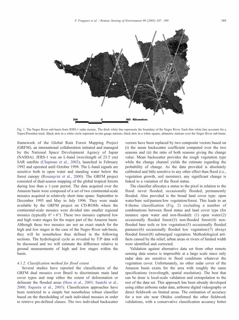
framework of the Global Rain Forest Mapping Project
(GRFM), an international collaboration initiated and managed
by the National Space Development Agency of Japan
(NASDA). JERS-1 was an L-band (wavelength of 23.5 cm)
SAR satellite (Chapman et al., 2002), launched in February
1992 and operated until October 1998. The L-band signals are
sensitive both to open water and standing water below the
forest canopy (Rosenqvist et al., 2000). The GRFM project
consisted of dual-season mapping of the global tropical forests
during less than a 1-year period. The data acquired over the
Amazon basin were composed of a set of two continental-scale
mosaics acquired in relatively short time spans: September to
December 1995 and May to July 1996. They were made
available by the GRFM project on CD-ROMs where the
continental-scale mosaics were divided into smaller regional
mosaics (typically 6-6-). These two mosaics captured low
and high water stages for the major part of the Amazon basin.
Although these two mosaics are not an exact match for the
high and low stages in the case of the Negro River sub-basin,
they will be nonetheless thus defined in the following
sections. The hydrological cycle as revealed by T/P data will
be discussed and we will estimate the difference relative to
ground measurements of high and low stages within the
basin.
4.1.2. Classification method for flood extent
Several studies have reported the classification of the
GRFM dual mosaics over Brazil to discriminate main land
cover types and map either the extent of deforestation or
delineate the flooded areas (Hess et al., 2003; Saatchi et al.,
2000; Siqueira et al., 2003). Classification approaches have
been restricted to a simple but nonetheless robust classifier
based on the thresholding of each individual mosaics in order
to retrieve pre-defined classes. The two individual backscatter
vectors have been replaced by two composite vectors based on
(i) the mean backscatter coefficient computed over the two
seasons and (ii) the ratio of both seasons giving the change
value. Mean backscatter provides the rough vegetation type
while the change channel yields the estimate regarding the
probability of change. As the data provided is absolutely
calibrated and little sensitive to any other effect than flood (i.e.,
vegetation growth, soil moisture), any significant change is
linked to a variation of the flood status.
The classifier allocates a status to the pixel in relation to the
flood: never flooded; occasionally flooded; permanently
flooded. Also provided is the broad land cover type: open
water/bare soil/pasture/low vegetation/forest. This leads to an
8-theme classification (Fig. 2) excluding a number of
combinations between flood status and land cover type (for
instance open water and non-flooded): (1) open water/(2)
occasionally flooded forest/(3) non-flooded forest/(4) non-
flooded bare soils or low vegetation/(5) occasionally flooded
pastures/(6) occasionally flooded low vegetation/(7) always
flooded forest/(8) submerged vegetation. Methodological arti-
facts caused by the relief, urban areas or rivers of limited width
were identified and corrected.
Validation against alternative data set from other remote
sensing data source is impossible at a large scale since only
radar data are sensitive to flood conditions whatever the
vegetation cover. Unfortunately, no other radar cover of the
Amazon basin exists for the area with roughly the same
specifications (wavelength, spatial resolution). The best that
can be done is local-scale validation and extrapolation to the
rest of the data set. This approach has been already developed
using either airborne radar data, airborne digital videography or
direct fieldwork on limited areas. The estimation of accuracy
for a test site near Obidos confirmed the other fieldwork
validations, with a conservative classification accuracy better
Fig. 1. The Negro River sub-basin from JERS-1 radar mosaic. The thick white line represents the boundary of the Negro River. Each thin white line accounts for a
Topex/Poseidon track. Black dots in a white circle represent in-situ gauge stations, black dots in a white square, altimetric stations over the Negro River sub-basin.
F. Frappart et al. / Remote Sensing of Environment 99 (2005) 387–399 389

Fig. 3. Extent of inundation as estimated from JERS-1 low water acquisition (grey) and high water acquisition (black).
Fig. 2. Classification results for the Negro River basin on JERS-1 radar images.
F. Frappart et al. / Remote Sensing of Environment 99 (2005) 387–399390
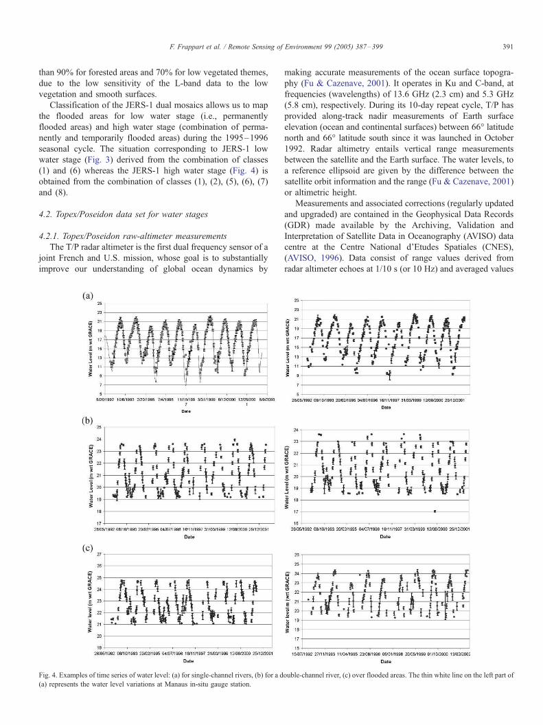
than 90% for forested areas and 70% for low vegetated themes,
due to the low sensitivity of the L-band data to the low
vegetation and smooth surfaces.
Classification of the JERS-1 dual mosaics allows us to map
the flooded areas for low water stage (i.e., permanently
flooded areas) and high water stage (combination of perma-
nently and temporarily flooded areas) during the 1995–1996
seasonal cycle. The situation corresponding to JERS-1 low
water stage (Fig. 3) derived from the combination of classes
(1) and (6) whereas the JERS-1 high water stage (Fig. 4) is
obtained from the combination of classes (1), (2), (5), (6), (7)
and (8).
4.2. Topex/Poseidon data set for water stages
4.2.1. Topex/Poseidon raw-altimeter measurements
The T/P radar altimeter is the first dual frequency sensor of a
joint French and U.S. mission, whose goal is to substantially
improve our understanding of global ocean dynamics by
making accurate measurements of the ocean surface topogra-
phy (Fu & Cazenave, 2001). It operates in Ku and C-band, at
frequencies (wavelengths) of 13.6 GHz (2.3 cm) and 5.3 GHz
(5.8 cm), respectively. During its 10-day repeat cycle, T/P has
provided along-track nadir measurements of Earth surface
elevation (ocean and continental surfaces) between 66- latitude
north and 66- latitude south since it was launched in October
1992. Radar altimetry entails vertical range measurements
between the satellite and the Earth surface. The water levels, to
a reference ellipsoid are given by the difference between the
satellite orbit information and the range (Fu & Cazenave, 2001)
or altimetric height.
Measurements and associated corrections (regularly updated
and upgraded) are contained in the Geophysical Data Records
(GDR) made available by the Archiving, Validation and
Interpretation of Satellite Data in Oceanography (AVISO) data
centre at the Centre National d’Etudes Spatiales (CNES),
(AVISO, 1996). Data consist of range values derived from
radar altimeter echoes at 1/10 s (or 10 Hz) and averaged values
Fig. 4. Examples of time series of water level: (a) for single-channel rivers, (b) for a double-channel river, (c) over flooded areas. The thin white line on the left part of
(a) represents the water level variations at Manaus in-situ gauge station.
F. Frappart et al. / Remote Sensing of Environment 99 (2005) 387–399 391

at 1s (or 1 Hz), corresponding to along-track ground spacing of
596 m and 5.96 km, respectively. The corrections applied in
this study are ionospheric, dry tropospheric, solid Earth tide,
and Pole tide corrections. From the two ionospheric corrections
available, we applied the onboard Doppler Orbitography and
Radiopositioning Integrated by Satellite (DORIS) based on the
measurement of the ionosphere electronic content (the dual-
frequency ionospheric correction, generally used in ocean
studies, is not valid over land). The wet tropospheric correction
is not applied in the present study. From the two tropospheric
corrections available, the first one, derived from the Topex
Microwave Radiometer (TMR) measurements of water vapour,
is unusable over land due to microwave emissions from
continental surfaces. The second one, derived from estimates
of atmospheric water vapour content by the General Circula-
tion Model (GCM) from the European Centre for Medium
Range Weather Forecast (ECMWF), is lacking in the AVISO
database. The lack of the wet tropospheric correction can lead
to an overestimation of the altimetric range up to 30 cm. The
spatial and temporal variations of the wet tropospheric
correction are assumed to be negligible within the Negro
River sub-basin (equatorial location and relatively small spatial
extent). The location of the satellite tracks over Negro River
basin is given in Fig. 1.
4.2.2. T/P time series construction
Each intersection between the river or flooded areas (as
determined by the SAR classification) and the satellite ground-
track defines a so-called ‘‘altimetric station’’, practically
defined as a rectangular window. In each cycle, the water
level at a given altimetric station is obtained by the
computation of the median of all the high-rate data (10 Hz)
included in the rectangular window. This process, repeated
every 10 days, allows the construction of the time series of
water level associated with each altimetric station. The
dispersion in L1 norm is given by the estimator known as
median absolute deviation (Eq. (1)):
MAD hð Þ ¼1
N 1
XN
i¼1
jhi hmedj ð1Þ
where MAD(h) is the mean absolute deviation of the
observations, N the number of observations, h i the ith
observation, and hmed the median of the observations.
Water levels are expressed with reference to geoid EIGEN-
GRACE02C. This geoid is derived from the first year of
GRACE space gravity mission measurements, which moni-
tored the time–space variations of the gravity field with a
resolution of 2-2- at the equator and an accuracy of 1 cm on
the geoid height (Reigber et al., 2005).
Examples of water level time series are given for different
types of water (Fig. 4):
– single-channel river,
– complex channel rivers: in this case, an altimeter virtual
station corresponds to each channel,
– flooded areas.
Fig. 4 shows a comparison between an altimetric time series
located 8.5 km upstream Manaus and the in-situ recorded water
levels at Manaus gauging station. In this example, the accuracy
of the T/P derived time-series is 27 cm.
The width of the rectangular window that defines the
altimetric station depends on the size of the flooded zone, but is
generally about 0.05-. When the dimension of the flooded area,
as is often the case, exceeds 0.05-, several altimetric stations
are defined. Increasing the number of altimetric stations
improves the sample size and leads to a better estimation of
water level variations at fine scales.
Fig. 5. Water level (m wrt GRACE geoid) map for JERS-1 low water acquisition.
F. Frappart et al. / Remote Sensing of Environment 99 (2005) 387–399392

4.2.3. In-situ time series construction
The Brazilian Water Agency (Agencia Nacional de Aguas or
ANA) is in charge of managing a network of 571 gauging
stations in the Brazilian part of the Amazon basin (http://
www.ana.gov.br). At each station, daily measurements of water
stage are collected and daily estimates of discharge are produced
using rating curves, obtained from periodic (sometimes several
times a year) simultaneous measurement of stage and discharge.
Among these 571 inventoried gauges, 46 are located in the
Negro River sub-basin and 25 of them have records over the last
20 years. The others have only temporary records that did not
include the 1995–1996. From these 25 in-situ gauge stations,
only 8 are located within the T/P groundtracks framework and
can, therefore be utilized, by interpolation of the river slope
between the two nearest T/P tracks, to estimate stage variation at
the altimetric stations (see their locations in Fig. 1).
4.3. Water level maps for high and low stages
Water level time series were available for 88 T/P altimetric
stations (Fig. 1). In addition, water level measurements from
eight in-situ leveled gauge stations are used to complete the
data set. Values for minimum and maximum water levels were
estimated at the date of the JERS mosaic. For each altimetric
Fig. 6. Water level (m wrt GRACE geoid) map for JERS-1 high water acquisition.
Fig. 7. Map of water level difference (m) between JERS-1 low and high water acquisition.
F. Frappart et al. / Remote Sensing of Environment 99 (2005) 387–399 393
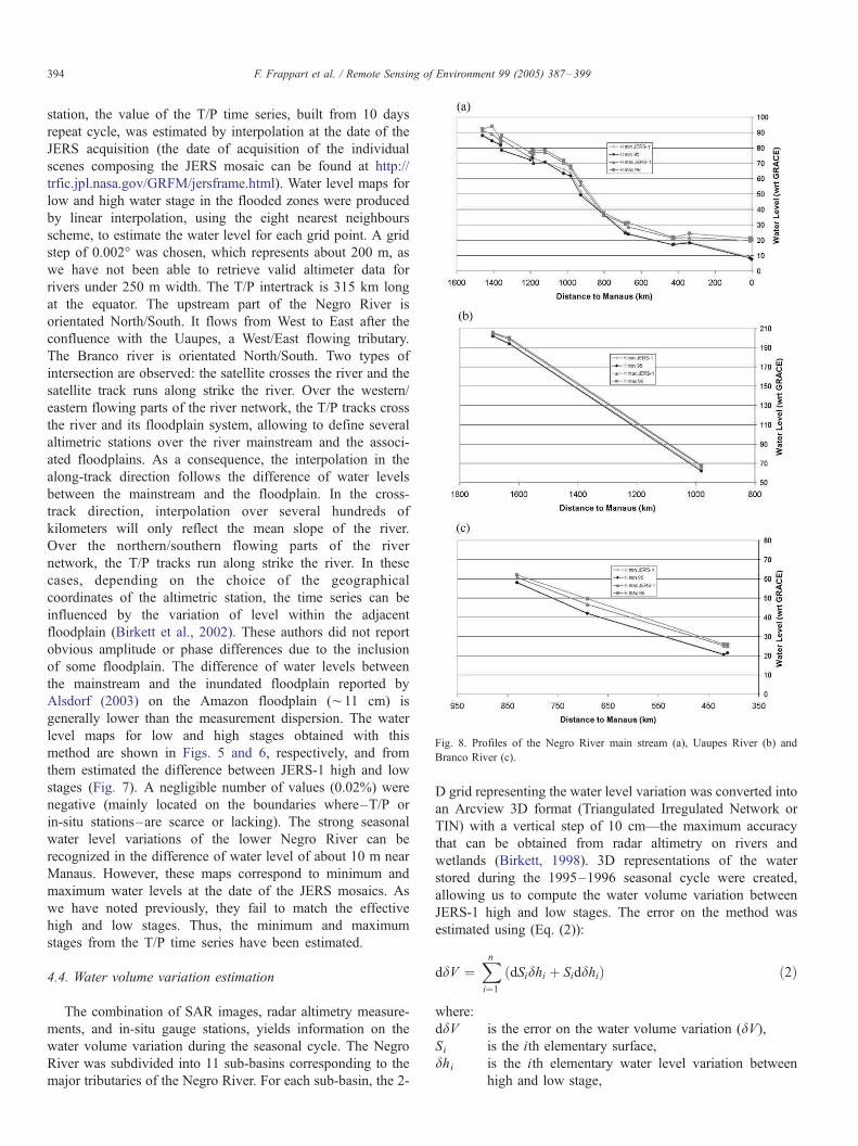
station, the value of the T/P time series, built from 10 days
repeat cycle, was estimated by interpolation at the date of the
JERS acquisition (the date of acquisition of the individual
scenes composing the JERS mosaic can be found at http://
trfic.jpl.nasa.gov/GRFM/jersframe.html). Water level maps for
low and high water stage in the flooded zones were produced
by linear interpolation, using the eight nearest neighbours
scheme, to estimate the water level for each grid point. A grid
step of 0.002- was chosen, which represents about 200 m, as
we have not been able to retrieve valid altimeter data for
rivers under 250 m width. The T/P intertrack is 315 km long
at the equator. The upstream part of the Negro River is
orientated North/South. It flows from West to East after the
confluence with the Uaupes, a West/East flowing tributary.
The Branco river is orientated North/South. Two types of
intersection are observed: the satellite crosses the river and the
satellite track runs along strike the river. Over the western/
eastern flowing parts of the river network, the T/P tracks cross
the river and its floodplain system, allowing to define several
altimetric stations over the river mainstream and the associ-
ated floodplains. As a consequence, the interpolation in the
along-track direction follows the difference of water levels
between the mainstream and the floodplain. In the cross-
track direction, interpolation over several hundreds of
kilometers will only reflect the mean slope of the river.
Over the northern/southern flowing parts of the river
network, the T/P tracks run along strike the river. In these
cases, depending on the choice of the geographical
coordinates of the altimetric station, the time series can be
influenced by the variation of level within the adjacent
floodplain (Birkett et al., 2002). These authors did not report
obvious amplitude or phase differences due to the inclusion
of some floodplain. The difference of water levels between
the mainstream and the inundated floodplain reported by
Alsdorf (2003) on the Amazon floodplain (¨11 cm) is
generally lower than the measurement dispersion. The water
level maps for low and high stages obtained with this
method are shown in Figs. 5 and 6, respectively, and from
them estimated the difference between JERS-1 high and low
stages (Fig. 7). A negligible number of values (0.02%) were
negative (mainly located on the boundaries where–T/P or
in-situ stations–are scarce or lacking). The strong seasonal
water level variations of the lower Negro River can be
recognized in the difference of water level of about 10 m near
Manaus. However, these maps correspond to minimum and
maximum water levels at the date of the JERS mosaics. As
we have noted previously, they fail to match the effective
high and low stages. Thus, the minimum and maximum
stages from the T/P time series have been estimated.
4.4. Water volume variation estimation
The combination of SAR images, radar altimetry measure-
ments, and in-situ gauge stations, yields information on the
water volume variation during the seasonal cycle. The Negro
River was subdivided into 11 sub-basins corresponding to the
major tributaries of the Negro River. For each sub-basin, the 2-
D grid representing the water level variation was converted into
an Arcview 3D format (Triangulated Irregulated Network or
TIN) with a vertical step of 10 cm—the maximum accuracy
that can be obtained from radar altimetry on rivers and
wetlands (Birkett, 1998). 3D representations of the water
stored during the 1995–1996 seasonal cycle were created,
allowing us to compute the water volume variation between
JERS-1 high and low stages. The error on the method was
estimated using (Eq. (2)):
ddV ¼Xn
i¼1
dSidhi þ Siddhið Þ ð2Þ
where:
ddV is the error on the water volume variation (dV),
Si is the ith elementary surface,
dhi is the ith elementary water level variation between
high and low stage,
Fig. 8. Profiles of the Negro River main stream (a), Uaupes River (b) and
Branco River (c).
F. Frappart et al. / Remote Sensing of Environment 99 (2005) 387–399394

dSi is the error on the ith elementary surface,
ddhi is the error on the ith elementary water level variation
between high and low stage.
The error sources include misclassifications, T/P altimetry
measurements and the linear interpolation method errors.
4.5. Estimation of half-peak flow integrated discharge
The half-flood peak time-integrated discharge represents the
volume of water that has flown into the mainstream during the
rising water period. It is defined as the ratio of the water
potential storage within the floodplain over the effective
volume of water that have been flowing into the mainstream
during the same period. The water potential storage is the result
of our method of estimation of water volume variation. The
effective water volume flowing into the main stream is the
time-integrated discharge between low stage of 1995 and the
peak flow of 1996 from each sub-basin. The discharge values
used in this study are derived from water levels recorded at in-
situ stations located at the mouth of each sub-basin.
5. Results and discussion
5.1. Spatial distribution of the inundated areas
The results obtained by the JERS dual mosaic for the Rio
Negro basin are given in Fig. 2. The total area subject to
flooding is 35,944 km2 for the JERS-1 low water acquisition
and 152,721 km2 for the JERS-1 high water acquisition.
Table 1 partitions flooded areas according to the type of
surface and vegetation. The results of flood mapping are
shown in Fig. 3 for JERS-1 low and high water stage. The two
maps highlight the importance of floodplains in the Negro
River sub-basin.
The different classes identified as inundated areas (perma-
nent or temporary) by the classifier are not evenly distributed
within the Negro River basin. This heterogeneous distribution
causes the great variety of situations observed during the high
and low water stages (Tables 2 and 3). Generally, the inundated
area is much wider (several times) during high water stage than
low water stage, except for the Carabinani sub-basin in which
20% of the surface is always flooded. Different behaviours can
be observed according to the geographical location of the sub-
basins. In the eastern part of the basin (Negro upstream and
Uaupes rivers), i.e., Cucui, Curicuriari, Sao Felipe and Serrinha
sub-basins, almost 5% of the basin is inundated during low
water stage and 2 to 3 times more during high water stage. The
situation is totally different in the northern part (Caracarai) and
downstream (Foz do Branco, Unini, Jau, Negro downstream):
the flooded area during high water stage is between 15% and
30% (increase factor greater than 4). With 12% and 54% of the
land being inundated during the low and high water stages,
respectively, the Branco river sub-basin differs from other
downstream sub-basins in terms of importance of inundated
areas. Its flow is controlled by the Negro River mainstem. As a
consequence, a high percentage of the sub-basin is always
inundated (up to 24% of the flooded areas of the Negro River
basin during high water stage).
5.2. High and low water levels
The T/P altimetry stations are unevenly distributed across
the basin (Fig. 1). Among the 88 T/P stations where water level
time series can be built, 34 are located on rivers and 54 on
wetlands. Five (four on the rivers and one on a flooded area)
are located on the Uaupes river flowing from the Colombian
part of the watershed, on the western side of the Negro basin.
This part of the basin is poorly known, no records from in-situ
gauges are available. Fifteen are located on the upper Negro,
near the Venezuelan border and the divide with Orinoco basin.
Table 1
Total areas of each class in the Negro river basin, based on JERS-1 SAR
mosaics from two dates
Class number Type of vegetation and flood Area (km2)
1 Open waters 14,100
2 Occasionally flooded forest 79,700
3 Non-flooded forest 510,650
4 Non-flooded bare soil or low vegetation 42,140
5 Occasionally flooded pastures 7560
6 Always flooded forest 21,860
7 Occasionally flooded low vegetation 29,530
8 Submerged vegetation during high water 6650
Table 2
Inundated areas, water volume variations (DV) between JERS-1 high and low water stages, and half peak flow integrated discharge for each sub-basin of Negro River
basin
Watershed Total area (km2) Inundated area (km2) Inundated/total (%) DV (km3) 1/2 peak flow (km3) 1/2 PF/DV
Jau 9040 665 7.4 1.8
Curicuriari 12,600 1,010 8.0 2.0 9.4 4.7
Carabinani 6970 620 8.9 1.8
Unini 23,770 2480 10.4 6.0
Negro downstream 77,530 9920 12.8 38.8
Cucui 70,740 12,140 17.1 16.2 64.7 4.0
Caracarai 120,350 23,580 19.6 42.2 51.6 1.2
Serrinha 157,950 35,220 22.3 57.0 84.0 1.5
Foz Branco 109,350 28,150 25.7 51.8
Sao Felipe 48,350 17,740 36.7 26.7 29.4 1.1
Branco 75,510 47,430 62.8 86.8
Downstream 302,170 89,270 29.5 187.0 302.5 1.6
F. Frappart et al. / Remote Sensing of Environment 99 (2005) 387–399 395
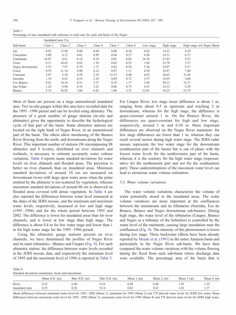
Most of them are present on a large unmonitored inundated
area. Two in-situ gauges within this area have recorded data for
the 1995–1996 period and can be leveled using altimetry. The
presence of a great number of gauge stations (in-situ and
altimetric) gives the opportunity to describe the hydrological
cycle of that part of the basin. Some altimetric stations are
located on the right bank of Negro River, in an unmonitored
part of the basin. The others allow monitoring of the Branco
River flowing from the north, and downstream along the Negro
River. This important number of stations (96 encompassing 88
altimetric and 8 in-situ), distributed on river channels and
wetlands, is necessary to estimate accurately water volume
variations. Table 4 reports mean standard deviations for water
levels on river channels and flooded areas. The precision is
better on river channels than on inundated areas. Minimum
standard deviations of around 10 cm are measured on
downstream rivers with large open water areas when the pulse
emitted by the altimeter is not scattered by vegetation, whereas
maximum standard deviations of around 60 cm is observed on
flooded areas covered with dense vegetation. In Table 4 are
also reported the differences between water level measured at
the dates of the JERS mosaic, and the minimum and maximum
water levels, respectively, measured at low and high stage
(1995–1996) and for the whole period between 1992 and
2002. The difference is lower for inundated areas than for river
channels, and is lower at low stage than high stage. The
difference is about 0.4 m for low water stage and lower than 1
m for high water stage for the 1995–1996 period.
Using the altimetric gauge stations present on river
channels, we have determined the profiles of Negro River
and its main tributaries—Branco and Uaupes (Fig. 8). For each
altimetric station, the difference between water levels recorded
at the JERS mosaic date, and respectively the minimum level
of 1995 and the maximum level of 1996 is reported in Table 5.
For Uaupes River, low stage mean difference is about 1 m,
ranging from about 0.5 m upstream and reaching 2 m
downstream, whereas for the high stage, the difference is
quasi-constant around 1 m. On the Branco River, the
differences are quasi-constant for high and low stage,
respectively, around 1 m and 0.30 m. More important
differences are observed on the Negro River mainstem: for
low stage differences are lower than 1 m, whereas they can
reach several meters during high water stage. The JERS radar
mosaic represents the low water stage for the downstream
(southeastern part of the basin) but is out of phase with the
lowest water levels for the northwestern part of the basin,
whereas it is the contrary for the high water stage (represen-
tative for the northeastern part and not for the southeastern
part). These underestimations of the maximum water level can
lead to erroneous water volume estimation.
5.3. Water volume variations
The water volume variations characterize the volume of
water potentially stored in the inundated areas. The water
volume variations are more important at the confluences
between the mainstream and its tributaries (Serrinha, Foz do
Branco, Branco and Negro downstream sub-basins). During
high stage, the water level of the tributaries (Uaupes, Branco
and Negro as a tributary of the Solimoes) is controlled by the
water level of the mainstem, causing large inundation near the
confluences (Fig. 9). The intensity of this phenomenon is lower
during low stage. These backwater effects have been already
reported by Meade et al. (1991) in the entire Amazon basin and
particularly in the Negro River sub-basin. We have then
compared the water volume variations with the volume flowing
during the flood from each sub-basin where discharge data
were available. The percentage area of the basin that is
Table 3
Percentage of area inundated with reference to total area for each sub-basin of the Negro
Inundated area (%)
Sub-basin Class 1 Class 2 Class 5 Class 6 Class 7 Class 8 Low stage High stage High stage wrt Negro Basin
Jau 0.02 12.90 0.00 0.60 0.00 0.20 0.62 14.33 6.29
Curicuriari 5.09 8.12 0.01 0.99 0.04 0.27 6.08 14.51 6.37
Carabinani 16.07 4.61 0.14 0.19 0.01 0.02 16.26 21.03 9.23
Unini 0.11 10.43 0.02 1.58 0.05 0.52 1.69 12.70 5.57
Negro downstream 3.53 7.97 0.79 1.73 0.42 0.54 5.26 14.97 6.57
Cucui 0.39 11.18 0.00 4.12 0.07 1.11 4.50 16.87 7.40
Caracarai 2.07 2.10 4.59 2.18 15.31 0.40 4.25 26.65 11.69
Serrinha 1.19 6.43 0.14 2.38 0.09 0.72 3.57 10.95 4.80
Foz Branco 0.41 14.24 0.31 3.57 8.32 1.37 3.98 28.21 12.37
Sao Felipe 1.22 8.96 0.10 3.25 0.06 0.75 4.47 14.33 6.29
Branco 5.19 36.92 1.06 6.82 1.88 2.35 12.01 54.23 23.79
Table 4
Standard deviations (minimum, mean and maximum)
Mean S.D. (m) Max S.D. (m) Min S.D. (m) Mean 1 (m) Mean 2 (m) Mean 3 (m) Mean 4 (m)
River 0.22 0.40 0.10 0.98 0.40 1.95 1.55
Inundated area 0.25 0.56 0.14 0.82 0.42 1.83 1.37
Mean differences between minimum water level for 1992–2002 (Mean 1), minimum for 1995 (Mean 2) and T/P derived water levels for JERS low water. Mean
differences between maximum water level for 1992–2002 (Mean 3), maximum water level for 1996 (Mean 4) and T/P derived water levels for JERS high water.
F. Frappart et al. / Remote Sensing of Environment 99 (2005) 387–399396

inundated at high water stage is inversely related to the ratio
between the flown water volume and the stored water volume,
i.e. the storage capacity of the floodplains is related to their
extent. But this relation is not proportional, and the storage
capacity of the floodplains cannot be inferred from their spatial
extent (Fig. 9 and Table 2). The nonlinear relationship between
potential storage capacity within the floodplain and flown
water volume during the flood is somewhat related to the
residence time of the water in the floodplain. This ratio can be
considered as a global indicator of the basin behaviour during
flooding processes.
Using Eq. (2) and taking into account the different sources
of error, we have estimated the minimum and maximum
storage. For the whole basin, we obtained a minimum change
in water storage 26% lower than our estimation and a
maximum change 34% greater.
6. Conclusion
For the first time, the combined use of altimetric water level
observations and inundation patterns to determine water
volume variations provides valuable information on the
inundation dynamics of river floodplains. In this study, we
calculated the water storage changes during the 1995–1996
hydrological cycle of the Negro River. It corresponds to a
volume variation of 331 km3 for the whole floodplain. This
result was compared with the water volume flown during the
flood. The storage capacity of the floodplain cannot be derived
from their extent. The potential storage capacity within the
floodplain is not proportional to the flown water during the
flood.
The use of the GRFM dual-season mosaics of JERS-1 SAR
images allows to accurately map (with a resolution of 100 m)
the Negro River basin according to the type of vegetation and
the inundation status. The classification results were used to
delineate flood extent at high and low stage. Unfortunately, the
date of acquisition of the mosaics may not coincide with the
real maxima (respectively minima) registered during the
hydrological cycle. Characterization of the seasonal and
interannual variation of inundation could be improved for
low vegetated areas combining JERS with other sensors
(Radarsat and ASAR for radar imagery or SPOT VGT, MODIS
and MERIS for multispectral imagery).
Satellite radar altimetry has the ability to monitor variations
in water level over wetlands, rivers and associated floodplains.
It represents a unique source of data for floodplain, as the in-
situ data records are generally located on the river mainstream.
Although the radar altimetric measurements are still suffering
severe limitations (Birkett, 1998; Birkett et al., 2002), the
capability to sample, from one cycle to another, both
mainstream and floodplain is a clear advantage compared with
traditional in-situ measurements. This aspect is essential
because it has been shown that the water volume stored in
Table 5
Differences between water levels at the dates of the JERS mosaic (1995 for low
water stage or 1996 for high water stage) and minimum for 1995, maximum
1996 for each T/P altimetric station over river channels
River Track Differences
1995 (m)
Differences
1996 (m)
Mean
1995
(m)
Mean
1996
(m)
Uaupes T/P 191 0.70 0.71 1.03 1.01
Uaupes T/P 102 0.44 1.29
Uaupes/Negro T/P 89 1.95 1.04
Negro T/P 89 0.75 1.04 0.40 2.06
Negro T/P 89 0.05 5.08
Negro T/P 254 0.43 1.70
Negro T/P 89 0.01 2.89
Negro T/P 89 0.09 3.50
Negro T/P 89 0.00 2.82
Negro T/P 89 0.05 1.24
Negro/Uaupes T/P 89 1.95 1.04
Negro T/P 254 0.00 1.30
Negro T/P 165 0.39 2.78
Negro T/P 76 0.06 0.70
Negro T/P 76 0.31 0.48
Negro T/P 241 0.72 2.57
Negro T/P 63 0.81 1.69
Branco T/P 241 0.26 1.21 0.23 0.91
Branco T/P 241 0.35 0.73
Branco T/P 241 0.08 0.78
Fig. 9. Water volume variation in the Negro River sub-basin.
F. Frappart et al. / Remote Sensing of Environment 99 (2005) 387–399 397

floodplains cannot be inferred from the flood extent, nor the
elevation of the flood by its extent. On the contrary, it seems
that significant geographical discrepancies exist in the way the
flood extends with increasing water level. Better results of
water cycle monitoring can be expected from a better sampling
both in time and space. To achieve this goal, the combination
of data from the present radar altimeters (T/P, ERS-1 and 2,
Jason-1, ENVISAT RA-2) can be useful. With the current
altimeters, the difference in water level between the rivers and
the associated floodplains is lower or equal to the dispersion of
the measurements. The next generation of altimeters (Cryosat,
Jason-2, the Water mission) is expected to provide a better
accuracy. Thus, the choice of the geographical range reflects
the nature of the selected target and a clear distinction between
rivers and the associated floodplains can be achieved.
Acknowledgements
This study was undertaken within the framework of a
collaboration between the Geodesie, Oceanographie et Hydro-
logie Spatiale (GOHS) team at Laboratoire d’Etudes en
Geophysique et Oceanographie Spatiales (LEGOS) and Labor-
atoire des Mecanismes et Transferts en Geologie (LMTG) for
the CASH (Contribution de l’Altimetrie Satellitaire pour
l’Hydrologie) project (reference 04 T 131). The authors would
like to acknowledge the Centre de Topographie des Oceans et
de l’Hydrosphere (CTOH) at LEGOS for the provision of the
Topex/Poseidon GDR data set and the HYBAM project for the
in-situ gauge measurements. We are particularly grateful to
thank Guy Lemichel for reviewing the English version of the
paper. We express our gratitude to an anonymous reviewer for
his very helpful comments and corrections. One of the authors,
F.F. was supported by a grant from Centre National d’Etudes
Spatiales (CNES, France) and Alcatel Space.
References
Alsdorf, D. E. (2003). Water storage of the central Amazon floodplain
measured with GIS and remote sensing imagery. Annals of the Association
of American Geographers, 93(1), 55–66.
Alsdorf, D. E., Melack, J. M., Dunne, T., Mertes, L. A. K., Hess, L. L., &
Smith, L. C. (2000). Interferometric radar measurements of water level
changes on the Amazon floodplain. Nature, 404, 174–177.
Alsdorf, D. E., Smith, L. C., & Melack, J. M. (2001). Amazon floodplain water
level changes measured with interferometric SIR-C radar. IEEE Transac-
tions on Geoscience and Remote Sensing, 39(2), 423–431.
AVISO. (1996). AVISO user handbook: Merged TOPEX/POSEIDON products,
AVI-NT-02-101-CN (3rd ed). Toulouse, France’ CNES 194 pp.
Bates, P. H. (2000). A simple raster-based model for flood inundation
simulation. Journal of Hydrology, 236, 54–77.
Birkett, C. M. (1998). Contribution of the TOPEX NASA radar altimeter to the
global monitoring of large rivers and wetlands. Water Resources Research,
34(5), 1223–1239.
Birkett, C. M., Mertes, L. A. K., Dunne, T., Costa, M. H., & Jasinski, M. J.
(2002). Surface water dynamics in the Amazon Basin: Application of
satellite radar altimetry. Journal of Geophysical Research, 107(D20),
8059–8080.
Chapman, B., Siqueira, P., & Freeman, A. (2002). The JERS Amazon
Multi-season Mapping Study (JAMMS): Observation strategies and
data characteristics. International Journal of Remote Sensing, 23(7),
1427–1446.
de Oliveira Campos, I., Mercier, F., Maheu, C., Cochonneau, G., Kosuth, P.,
Blitzkow, D., et al. (2001). Temporal variations of river basin waters from
Topex/Poseidon satellite altimetry; application to the Amazon basin.
Comptes Rendus del Academie des Sciences, Paris, Sciences de la Terre
et des Planetes, 333, 1–11.
Frazier, P., Page, K., Louis, J., Briggs, S., & Robertson, A. I. (2003). Relating
wetland inundation to river flow using Landsat TM data. International
Journal of Remote Sensing, 24(19), 3755–3770.
Fu, L. L., & Cazenave, A. (2001). Satellite altimetry and Earth science, a
handbook of techniques and applications. London, U.K.’ Academic Press.
Hamilton, S. K., Sippel, S. J., & Melack, J. M. (2002). Comparison of
inundation patterns among major South American floodplains. Journal of
Geophysical Research, 107(D20), 10.129–10.143.
Hayashi, M., & van der Kamp, G. (2000). Simple equations to represent the
volume area depth relations of shallow wetlands in small topographic
depressions. Journal of Hydrology, 237, 74–85.
Hess, L. L., Melack, J. M., Filoso, S., & Wang, Y. (1995). Delineation of
inundated area and vegetation along the Amazon floodplain with SIR-C
synthetic aperture radar. IEEE Transactions on Geoscience and Remote
Sensing, 33, 896–904.
Hess, L. L., Melack, J. M., Novo, E.M.L.M., Barbosa, C. C. F., & Gastil, M.
(2003). Dual-season mapping of wetland inundation and vegetation for the
central Amazon basin. Remote Sensing of Environment, 87(4), 404–428.
Junk, W., Bayley, P. B., & Sparks, R. E. (2003). The flood pulse concept in
river floodplain systems. In D. P. Dodge (Ed.), Proceedings of the
international large river symposium. Can. Spec. Pub. Fish. Aquat. Sci.,
vol. 106 (pp. 110–127).
Liebmann, B., & Marengo, J. A. (2001). Interannual variability of the rainy
season and rainfall in the Brazilian Amazon basin. Journal of Climate, 14,
4308–4318.
Maheu, C., Cazenave, A., & Mechoso, C. R. (2003). Water level fluctuations in
the Plata basin (South America) from Topex/Poseidon satellite altimetry.
Geophysical Research Letters, 30(3), 1143–1146.
Marengo, J. A., Liebmann, B., Kousky, V. E., Filizola, & Wainer, I. C. (2001).
Onset and end of the rainy season in the Brazilian Amazon basin. Journal of
Climate, 14, 833–852.
Meade, R. H., Rayol, J. M., da Conceicao, S. C., & Natividade, J. R. G. (1991).
Backwater effects in the Amazon River basin of Brazil. Environmental
Geology and Water Sciences, 18(2), 105–114.
Mertes, L. A. K. (1997). Documentation and significance of the perirheic zone
on inundated floodplains. Water Resources Research, 33(7), 1749–1762.
Mertes, L. A. K., Daniel, D. L., Melack, J. M., Nelson, B., Martinelli, L. A., &
Forsberg, B. R. (1995). Spatial patterns of hydrology, geomorphology, and
vegetation on the floodplain of the Amazon River in Brazil from remote
sensing perspective. Geomorphology, 13, 215–232.
Priestnall, G., Jaafar, J., & Duncan, A. (2000). Extracting urban features from
LIDAR-derived digital surface models. Computers, Environment and
Urban Systems, 24, 65–78.
Reigber, C., Schmidt, R., Flechtner, F., Konig, R., Meyer, U., Neumayer, K.
H., et al. (2005). An Earth gravity field model complete to degree and
order 150 from GRACE: EIGEN-GRACE02S. Journal of Geodynamics,
39(1), 1–10.
Richards, J. A., Sun, G. Q., & Simonetti, D. S. (1987). L-band radar backscatter
modeling of forest stands. IEEE Transactions on Geoscience and Remote
Sensing, 25, 487–498.
Richey, J. E., Nobre, C., & Deser, C. (1989). Amazon River discharge and
climate variability: 1903 to 1985. Science, 246, 101–102.
Richey, J. E., Melack, J. M., Aufdenkampfe, A. K., Ballester, V. M., & Hess, L.
L. (2002). Outgassing from Amazonian rivers and wetlands as a large
tropical source of atmospheric CO2. Nature, 617. doi:10.1038/416617a.
Rosenqvist, A., Shimada, M., Chapman, B., Freeman, A., de Grandi, G.,
Saatchi, S., et al. (2000). The Global Rain Forest Mapping project—a
review. International Journal of Remote Sensing, 21(6&7), 1375–1387.
Saatchi, S. S., Nelson, B., Podest, E., & Holt, J. (2000). Mapping Land-cover
types in the Amazon Basin using 1 km JERS-1 mosaic. International
Journal of Remote Sensing, 21(6&7), 1201–1234.
Sippel, S. J., Hamilton, S. K., Melack, J. M., & Novo, E. M. M. (1998). Passive
microwave observations of inundation area and the area/stage relation in the
F. Frappart et al. / Remote Sensing of Environment 99 (2005) 387–399398

Amazon River floodplain. International Journal of Remote Sensing, 19,
3055–3074.
Siqueira, P., Chapman, B., & McGarragh, G. (2003). The coregistration,
calibration, and interpretation of multiseason JERS-1 SAR data over South
America. Remote Sensing of Environment, 87, 389–403.
Smith, L. C. (1997). Satellite remote sensing of river inundation area, stage and
discharge: A review. Hydrological Processes, 11, 1427–1439.
Smith, L. C., Isacks, B. L., Bloom, A. L., & Murray, A. B. (1996). Estimation
of discharge from three braided rivers using synthetic aperture radar
imagery: Potential application to ungauged basins. Water Resources
Research, 32(7), 2031–2034.
Smith, L. C., Isacks, B. L., Forster, R. R., Bloom, A. L., & Preuss, I.
(1995). Estimation of discharge from braided glacial rivers using ERS 1
synthetic aperture radar: First results. Water Resources Research, 31(5),
1325–1329.
Sternberg, H. (1975). The Amazon River of Brazil. Geographische, 1–74.
Townshend, P. A., & Walsh, S. J. (1998). Modelling floodplain inundation
using an integrated GIS with radar and optical remote sensing. Geomor-
phology, 21, 295–312.
Townsend, P. A., & Foster, J. R. (2002). A synthetic aperture radar-based model
to assess historical changes in lowland hydroperiod. Water Resources
Research, 38(7), W1115. doi:10.1029/2001WR001046.
Toyra, J., Pietroniro, A., & Martz, L. W. (2001). Multisensor hydrologic
assessment of a freshwater wetland. Remote Sensing of Environment, 75,
162–173.
Usachev, V. F. (2002). Evaluation of flood plain inundations by remote
sensing methods. Proceedings of the Hamburg symposium. IAHS pub, vol.
145 (pp. 475–482).
Wang, Y., Hess, L. L., Filoso, S., & Melack, J. M. (1995). Understanding the
radar backscattering from flooded and non-flooded Amazonian forests:
Results from canopy backscatter modelling. Remote Sensing of Environ-
ment, 54, 324–332.
F. Frappart et al. / Remote Sensing of Environment 99 (2005) 387–399 399

Hydrologie spatiale : Développement d’outils méthodologiques pour l’utilisation de la télédétection sur les grands bassins fluviaux
Chapitre 6 : Variations de volume d’eau de surface dans les grands bassins fluviaux
102
3. Variations inter-annuelles de volume d’eau de surface dans la
partie avale du bassin du Mékong
3.1 Caractéristiques hydrologiques de la zone étudiée
Le basin du Mékong est le plus grand basin versant d’Asie du Sud Est avec une superficie de
795 000 km² [IMC, 1988], où vivent 65 millions d’habitants [MRC et UNEP, 1997]. Le
Mékong prend sa source sur le plateau tibétain et traverse six pays (la Chine, Burma, le Laos,
la Thaïlande, le Cambodge et le Vietnam) avant de se jeter dans le sud de la mer de Chine.
Avec un débit moyen annuel de 475 000 m3 et une longueur totale de 4800 km, il est le
dixième fleuve du monde en terme de débit et le cinquième plus long.
La partie avale du bassin du Mékong, qui draine une surface totale de 606 000 km², soit 77%
de la surface du bassin, est considérée comme la partie la plus importante du bassin aussi d’un
point de vue environnemental qu’économique [IMC, 1988 ; Hori, 2000]. La zone d’étude est
la partie avale du bassin du Mékong, et son delta, situés au Cambodge et au Vietnam.
Le Mékong se divise en trois branches au niveau de Pnohm Penh : le Tonle Sap, le Bassac et
le Mékong inférieur. Durant la crue, l’eau est drainée du Mékong et du Bassac jusqu’au lac de
Tonle Sap à travers le Tonle Sap, tandis que dès la décrue s’amorce, le phénomène inverse se
produit. Ce renversement du flot est une caractéristique unique au monde qui est la cause
d’une diminution du débit du Mékong moins marquée pendant la saison sèche [Hoanh et al.,
2003]. Après la frontière vietnamienne, le Mékong se divise en plusieurs tronçons formant un
delta. Le bassin du Mékong est présenté sur la Figure 6-6 avec la couverture spatiale de TP et
d’ERS-1&2/ENVISAT.
Le régime hydrologique du Mékong est gouverné par les conditions climatiques et par
l’alternance d’une saison sèche et d’une saison des pluies, dues au phénomène de mousson.
Les vents soufflent du sud ouest durant la saison des pluies, qui s’étend de mai à octobre avec
un pic en septembre, et du nord est durant la saison sèche.

Hydrologie spatiale : Développement d’outils méthodologiques pour l’utilisation de la télédétection sur les grands bassins fluviaux
Chapitre 6 : Variations de volume d’eau de surface dans les grands bassins fluviaux
103
3.2 Délimitation des zones inondées
Le capteur VEGETATION (VGT), embarqué sur le satellite SPOT-4, a été conçu pour
observer, comme son nom l’indique, l’évolution de la végétation et les surfaces continentales
[Arnaud et Leroy, 1991]. Il effectue des acquisitions de réflectance dans quatre bandes
spectrales, B0 (bleu, 430-470 nm), B2 (rouge, 610-680 nm), B3 (proche infra-rouge, 780-890
nm) et PIR (proche infra-rouge, 1580-1750 nm) pour réaliser des images grand champ. Grâce
à sa fauchée large de 2250 km, VGT réalise une couverture journalière du globe à la
résolution spatiale d’un kilomètre [Xiao et al., 2002].
Figure 6-6: Le bassin du Mékong et couverture spatiale de T/P (jaune) et ERS-2/ENVISAT (rouge).
Les points blancs représentent les stations virtuelles ERS-2/ENVISAT, les étoiles jaunes les stations
virtuelles dont les résultats sont présentés ultérieurement, les cercles blancs correspondent aux
comparaisons T/P et ERS-2/ENVISAT.

Hydrologie spatiale : Développement d’outils méthodologiques pour l’utilisation de la télédétection sur les grands bassins fluviaux
Chapitre 6 : Variations de volume d’eau de surface dans les grands bassins fluviaux
104
Trois produits standards sont fournis aux utilisateurs : les produits bruts (VGT-P), les
synthèses journalières (VGT-S1) et à dix jours (VGT-S10). Les paramètres de surface issues
des données VGT-S10 sont couramment employés pour le suivi des cultures et des forêts,
l’étude des variations de masse et des cycles biogéochimiques et sont assimilés dans les
modèles de prévision météorologique [Duchemin et al., 2002].
Ces données permettent de calculer l’indice de végétation, défini par Tucker [1979] pour
suivre l’évolution du couvert végétal ou NDVI (Normalized Difference Vegetation Index):
2323
BBBBNDVIVGT +−= (Eq. 6-1)
L’application d’un seuil permet de délimiter les zones d’inondation. Sur les eaux libres, les
valeurs du NDVI sont quasiment nulles. Les valeurs du NDVI des pixels correspondant à des
lacs ou des fleuves sont égales à -0,1 dans le produit VGT-S10 (disponibles sur le site
http://free.vgt.vito.be/ entre mai 1998 et décembre 2004). Pendant la crue, l’eau submerge la
végétation basse et les rizières. Les valeurs du NDVI sont donc plus élevées sur les zones
inondées que sur les eaux libres. Nous supposons que les zones inondées ont des valeurs du
NDVI inférieures à 0,2. Des exemples de carte d’indice de végétation, permettant de se faire
un idée de l’évolution de l’inondation, sont présentés sur la Figure 6-7.
Figure 6-7: Cartes de NDVI provenant de VGT.

Hydrologie spatiale : Développement d’outils méthodologiques pour l’utilisation de la télédétection sur les grands bassins fluviaux
Chapitre 6 : Variations de volume d’eau de surface dans les grands bassins fluviaux
105
3.3 Cartes de hauteur d’eau
Les cartes d’inondation obtenues par seuillage nous ont permis de définir 80 stations virtuelles
ERS-2 et ENVISAT sur notre zone d’étude (Figure 6-6). Des exemples de séries temporelles
obtenues avec ENVISAT, dans différentes régions du bassin du Mékong, sont présentées sur
la Figure 6-8.
Figure 6-8: Exemples de séries temporelles ENVISAT dans le bassin du Mékong.
8
6
7
52
1
3 4
1
2
3
4
5
6
78

Hydrologie spatiale : Développement d’outils méthodologiques pour l’utilisation de la télédétection sur les grands bassins fluviaux
Chapitre 6 : Variations de volume d’eau de surface dans les grands bassins fluviaux
106
En raison des caractéristiques orbitales d’ERS-2 et d’ENVISAT (répétitivité de 35 jours), des
cartes d’inondation mensuelles ont été calculées à partir des cartes décadaires : elles
correspondent à l’union des pixels inondés à chacune des trois décades. Une interpolation
bilinéaire des hauteurs d’eau sur l’étendue des zones d’inondation conduit à la création de
cartes mensuelles de hauteur d’eau pour les années 1998-2003, entre juillet et décembre
(Figure 6-9 pour l’année 2003).
Figure 6-9 : Cartes d'inondation obtenues pour l'année 2003.
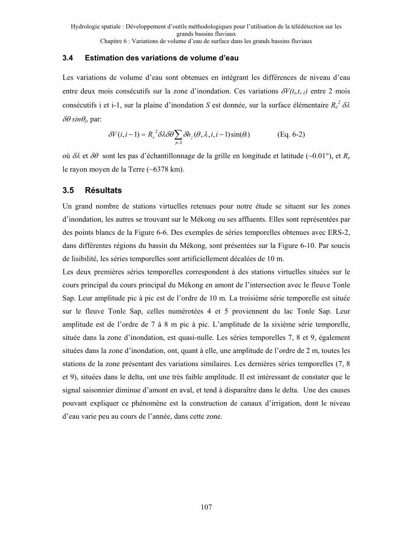
Hydrologie spatiale : Développement d’outils méthodologiques pour l’utilisation de la télédétection sur les grands bassins fluviaux
Chapitre 6 : Variations de volume d’eau de surface dans les grands bassins fluviaux
107
3.4 Estimation des variations de volume d’eau
Les variations de volume d’eau sont obtenues en intégrant les différences de niveau d’eau
entre deux mois consécutifs sur la zone d’inondation. Ces variations δV(ti,ti-1) entre 2 mois
consécutifs i et i-1, sur la plaine d’inondation S est donnée, sur la surface élémentaire Re2 δλ
δθ sinθj, par:
)sin()1,,,()1,( 2j
Sj
je iihRiiV θλθδδλδθδ ∑∈ −=− (Eq. 6-2)
où δλ et δθ sont les pas d’échantillonnage de la grille en longitude et latitude (~0.01°), et Re
le rayon moyen de la Terre (~6378 km).
3.5 Résultats
Un grand nombre de stations virtuelles retenues pour notre étude se situent sur les zones
d’inondation, les autres se trouvant sur le Mékong ou ses affluents. Elles sont représentées par
des points blancs de la Figure 6-6. Des exemples de séries temporelles obtenues avec ERS-2,
dans différentes régions du bassin du Mékong, sont présentées sur la Figure 6-10. Par soucis
de lisibilité, les séries temporelles sont artificiellement décalées de 10 m.
Les deux premières séries temporelles correspondent à des stations virtuelles situées sur le
cours principal du cours principal du Mékong en amont de l’intersection avec le fleuve Tonle
Sap. Leur amplitude pic à pic est de l’ordre de 10 m. La troisième série temporelle est située
sur le fleuve Tonle Sap, celles numérotées 4 et 5 proviennent du lac Tonle Sap. Leur
amplitude est de l’ordre de 7 à 8 m pic à pic. L’amplitude de la sixième série temporelle,
située dans la zone d’inondation, est quasi-nulle. Les séries temporelles 7, 8 et 9, également
situées dans la zone d’inondation, ont, quant à elle, une amplitude de l’ordre de 2 m, toutes les
stations de la zone présentant des variations similaires. Les dernières séries temporelles (7, 8
et 9), situées dans le delta, ont une très faible amplitude. Il est intéressant de constater que le
signal saisonnier diminue d’amont en aval, et tend à disparaître dans le delta. Une des causes
pouvant expliquer ce phénomène est la construction de canaux d’irrigation, dont le niveau
d’eau varie peu au cours de l’année, dans cette zone.

Hydrologie spatiale : Développement d’outils méthodologiques pour l’utilisation de la télédétection sur les grands bassins fluviaux
Chapitre 6 : Variations de volume d’eau de surface dans les grands bassins fluviaux
108
La Figure 6-11 présente les variations mensuelles de volume d’eau de surface obtenues par la
méthode présentée ci-dessus de 1998 à 2003. Seules figurent les variations entre août et
décembre (période de hautes eaux). En effet, hors des périodes d’inondation, la signature de la
végétation est dominant, seul le fleuve est visible sur les images VGT. Des variations
positives de volume d’eau sont observées entre août et octobre. Ces variations ont été plus
Figure 6-10: Exemples de séries temporelles obtenues avec ERS-2 dans le
bassin du Mékong.

Hydrologie spatiale : Développement d’outils méthodologiques pour l’utilisation de la télédétection sur les grands bassins fluviaux
Chapitre 6 : Variations de volume d’eau de surface dans les grands bassins fluviaux
109
importantes pour les années 2000 à 2002 que pour les années 1998, 1999 et 2003, avec des
variations de volume pouvant atteindre 15 km3 voire 25 km3 entre septembre et août 2002.
3.6 Article “Water volume change in the lower Mekong basin from satellite
altimetry and other remote sensing data”
Cette étude a fait l’objet d’un article soumis à Geophysical Journal International, actuellement en révision.
Figure 6-11: Variations de volume d'eau de surface obtenues par altimétrie et imagerie.

Hydrologie spatiale : Développement d’outils méthodologiques pour l’utilisation de la télédétection sur les grands bassins fluviaux
Chapitre 6 : Variations de volume d’eau de surface dans les grands bassins fluviaux
110
WATER VOLUME CHANGE IN THE LOWER MEKONG
FROM SATELLITE ALTIMETRY
AND OTHER REMOTE SENSING DATA
F. Frappart1, K. DoMinh
1, J. L’Hermitte
2, A. Cazenave
1,
G. Ramillien1T. LeToan
2 and N. Mognard-Campbell
1
1. LEGOS-CNES, 18 av. E. Belin, 31401 Toulouse Cedex 9, France
2. CESBIO-CNES, 18 av. E. Belin, 31401 Toulouse Cedex 9, France
October 2005
Corresponding Author :
F. Frappart, LEGOS-CNES, 18 av. E. Belin, 31401 Toulouse Cedex 9, France
Tel : 33 5 61 33 29 25
Fax : 33 5 61 25 32 05
Email : [email protected]

Hydrologie spatiale : Développement d’outils méthodologiques pour l’utilisation de la télédétection sur les grands bassins fluviaux
Chapitre 6 : Variations de volume d’eau de surface dans les grands bassins fluviaux
111
Abstract
Satellite altimetry data from the ERS-2, ENVISAT satellites have been analysed to construct
water level time series (for 1996-2003) over the lower Mekong River basin. The study area
includes the Tonle Sap Lake, seasonally inundated areas and several branches of the
hydrographic network of the Mekong delta. Very strong seasonal signal is reported over the
main river north of 13°N, the Tonle Sap Lake and Tonle Sap River, amplitude reaching 8-10
meters annually. Clear interannual signal is also visible. For example year 1999 corresponds
to weak floods, contrasting with year 2000 during which strong flood is noticed. Southward,
we also observe large seasonal fluctuations (2-3 m) over inundated floodplains, as identified
using imagery data from the SPOT 4 Vegetation instrument. Depending on the location, quite
different annual amplitudes are observed, the closer to the Mekong mouth, the smaller the
signal. We interpret this observation as the effect of dams built over the Delta in the recent
years/decades. Using NDVI data from SPOT-4/Vegetation, we study the annual extent of
flood plains in the delta. Then combining the area extent of floods with water levels estimated
from the ERS/ENVISAT data, we compute maps of monthly surface water volume change
over successive years (1996-2003). Averaged over the lower Mekong basin, this surface water
volume change is compared to the total (i.e., surface plus soil) water volume change inferred
from the GRACE satellite.

Hydrologie spatiale : Développement d’outils méthodologiques pour l’utilisation de la télédétection sur les grands bassins fluviaux
Chapitre 6 : Variations de volume d’eau de surface dans les grands bassins fluviaux
112
1. Introduction
The Mekong river, one of the largest river of the world, was considered to be almost in their
natural state (i.e. without interference from human influences) until recently. The annual
recurrence of the Monsoon floods, from August to November, is of great importance for
farming and economics activities. Between 80 % and 90 % of the freshwater use in the
Mekong basin is used for irrigating rice crops (MRC, 2002). Some years, vast regions are
flooded during several weeks, causing important damages. The year 2000, for instance, was
characterized by an especially severe flood, reported as the most devastating in the last 40
years.
Many methods have been employed to estimate the extent of inundation and a review of how
remote sensing is used to map inundation can be found in Smith (1997). In the lower Mekong
basin, the flood extent has been evaluated using SPOT quicklook mosaics (Chia et al., 2001).
Recently, a new methodology, based on the combine use of radar altimetry and satellite
imagery, was used to determine volume variations of surface water in the Negro river basin,
the main tributary of the Amazon river (Frappart et al., in press a). In this study, we apply a
similar method to monitor the volume variation of surface water during the flood and its
recede (August to December) in the lower Mekong basin from six years of SPOT Vegetation
multispectral imagery and ERS-2/ENVISAT radar altimetry.
2. Hydrological characteristics of the study area
The Mekong basin is the largest river basin in southeast Asia with an area of 795,000 km²
(IMC, 1988). It is the home for over 65 million inhabitants (MRC and UNEP, 1997). The
Mekong river has its source on the Tibetan Plateau and then flows through six countries
(China, Burma, Laos, Thailand, Cambodia and Vietnam) before reaching the south China Sea.
With a mean annual flow of 475 000 m3 and a total length 4800 km, it is the world’s tenth
greatest and twelfth longest respectively (IMC, 1988). The lower Mekong basin, which drains
a total catchment area of 606,000 km² (77 % of the basin), is considered as the most important
part of the Mekong basin, both environmentally and economically (IMC, 1988; Hori, 2000).
The study area is the lower Mekong and Delta Cambodia and Vietnam. At Phnom Penh, the
Mekong river divides into three parts: the Tonle Sap river, the Bassac River, and the lower
Mekong. During the flood season, water is drained from the Mekong and Bassac rivers into

Hydrologie spatiale : Développement d’outils méthodologiques pour l’utilisation de la télédétection sur les grands bassins fluviaux
Chapitre 6 : Variations de volume d’eau de surface dans les grands bassins fluviaux
113
the Tonle Sap lake, through the Tonle Sap river, and as the water level decreases in the
Mekong river, the water is drained from the Tonle Sap lake into the Mekong and Bassac
rivers. The reversal of the flow of the Tonle Sap river is a unique hydrological feature that is
responsible for a higher dry season flow for the Delta than if he only received water from the
Mekong river (Hoanh et al., 2003). When reaching the Vietnam border, the main river divides
into several branches which constitues the Mekong delta. This region is very flat and is
refered as to the Mekong lowlands. Fig.1 is a sketch of the study area.
The hydrological regime of the Mekong river is primarily dependent on the climatic
conditions of the alternating wet and dry season. Climate is governed by the moonson winds
that blows northeast or southwest depending on the period of the year. The southwest
moonson corresponds to the rainy season which ranges from May to October, with a peak in
September. Fig.2 shows the mode 1 of the Empirical Orthogonal Function (EOF)
decomposition of precipitation data over the lower Mekong, from 1996 to 2003 (the period of
analysis of this study; see below). The data used here are monthly 1°x1° gridded precipitation
of the Global Precipitation Climate Center (GPCC, Rudolf et al., 1994; Rudolf et al., 2003).
The temporal curve shows a clear annual cycle, peaking in September. The wettest region is
the southern uplands ans lowlands, south of the Tonle Sap Lake and northern part of the delta.
During the flood season, the Mekong river water drains into the Tonle Sap Lake, through the
Tonle Sap River. When the Melong water level goes down, water drains out from the lake
into the main river.
Superimposed to the annnual cycle, clear interannual fluctuations are visible. Fig.2 indicates
two rainy years: 1997 and 2000. The lowlands suffer annual floods during the rainy season.
During the rainy year 2000, a particularly devasting flood affected a very large area. This
event will be discussed below in some details.
3.Datasets
In this study, we use different datasets: altimetry data from the ERS-2, ENVISAT and
Topex/Poseidon (T/P) satellites for measuring water level changes, and NDVI data from the
Vegetation instrument onboard the SPOT satellites to determine the surface water extent over
inundated plains.
ERS-2 and ENVISAT and Topex/Poseidon altimetry data

Hydrologie spatiale : Développement d’outils méthodologiques pour l’utilisation de la télédétection sur les grands bassins fluviaux
Chapitre 6 : Variations de volume d’eau de surface dans les grands bassins fluviaux
114
ERS-2, launched in 1995 by the European Space Agency (ESA), is the successor of ERS-1
(1991-1996), designed to study the Earth environment. The satellite carries, among other
instruments, a radar altimeter developed for measuring sea surface height. However,
retracking of the raw altimeter waveforms (radar echoes) allows the use of the ERS data over
continental surface waters (Legrésy et al., 1995). Here we use only the ERS-2 retracked
altimetry data because the ERS-1 retracked data suffer too many gaps. The ERS-2 altimetry
time series (20 Hz data) starts in January 1995. The average intertrack spacing over the lower
Mekong basin is 85 km, while the revisit time (orbital cycle) is 35 days. The ENVISAT
satellite was launched on February 2002 for environmental objectives (Gardini et al.,
1995). The satellite’s payload includes a radar altimeter operating on two frequencies (RA-2).
Its orbital characteristics are similar to those of the ERS satellite (i.e., 35-day repeat cycle and
ground-track spacing of about 85 km). The RA-2 instrument provides radar echoes over
ocean, land and ice to measure sea surface height, surface water level variations over river
basins and ice surface elevation (Wehr and Attema, 2001). Processing of altimeter waveforms
is performed on ground to obtain accurate range values (Zelli, 1999). For the ENVISAT
mission, four different retrackers are operationally applied to RA-2 raw-data to provide
accurate height estimates. Each of them has been developed for a specific surface response :
one for ocean (ESA, 2002), two for ice sheets (Bamber, 1994 and Legrésy, 1995) and one for
sea ice (Laxon, 1994). In this study, we use the ENVISAT RA-2 20Hz range measurements
contained in the Geophysical Data Records (GDRs) (ESA, 2002) from cycle 12 to cycle 30 of
ENVISAT RA-2 Mission. As suggested by Frappart et al. (in press b), we use the range
measurements processed with the OCOG (or Ice-1) retracking scheme (Wingham et al., 1986;
Bamber, 1994).
As of mid-2002, we use the ENVISAT data instead of ERS-2. Figure 3 shows the ERS-
2/ENVISAT track coverage over the study area. On Fig. 3 are also superimposed the few
Topex/Poseidon (T/P) tracks of the former orbit. In effect in September 2002, a few months
after the launch of its successor, Jason-1, T/P moved to a new orbit, midway of the former
orbital tracks. We do not consider the latter data because of the too short time series available.
For T/P, we use the Geophysical Data Records (standard ocean data, AVISO data base) which
have been shown to be precise enough for continental water studies (e.g., Birkett, 1998,
Birkett et al., 2002; Maheu et al., 2003). The T/P orbital cycle is 10 days. Compared to the 35
days orbit cycle of ERS/ENVISAT, this is obviously more favourable to study water level
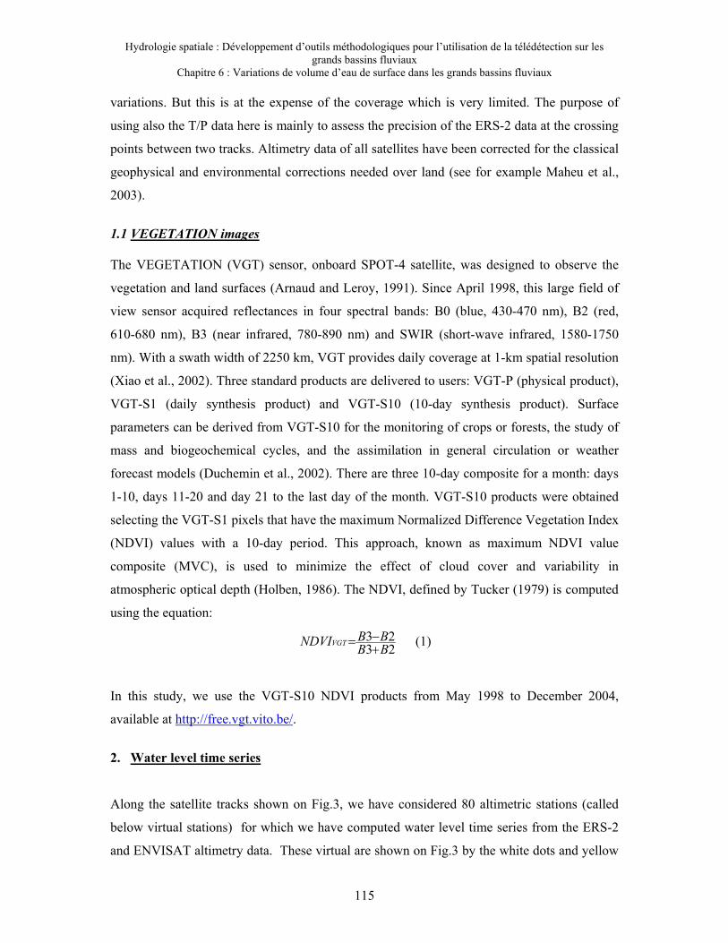
Hydrologie spatiale : Développement d’outils méthodologiques pour l’utilisation de la télédétection sur les grands bassins fluviaux
Chapitre 6 : Variations de volume d’eau de surface dans les grands bassins fluviaux
115
variations. But this is at the expense of the coverage which is very limited. The purpose of
using also the T/P data here is mainly to assess the precision of the ERS-2 data at the crossing
points between two tracks. Altimetry data of all satellites have been corrected for the classical
geophysical and environmental corrections needed over land (see for example Maheu et al.,
2003).
1.1 VEGETATION images
The VEGETATION (VGT) sensor, onboard SPOT-4 satellite, was designed to observe the
vegetation and land surfaces (Arnaud and Leroy, 1991). Since April 1998, this large field of
view sensor acquired reflectances in four spectral bands: B0 (blue, 430-470 nm), B2 (red,
610-680 nm), B3 (near infrared, 780-890 nm) and SWIR (short-wave infrared, 1580-1750
nm). With a swath width of 2250 km, VGT provides daily coverage at 1-km spatial resolution
(Xiao et al., 2002). Three standard products are delivered to users: VGT-P (physical product),
VGT-S1 (daily synthesis product) and VGT-S10 (10-day synthesis product). Surface
parameters can be derived from VGT-S10 for the monitoring of crops or forests, the study of
mass and biogeochemical cycles, and the assimilation in general circulation or weather
forecast models (Duchemin et al., 2002). There are three 10-day composite for a month: days
1-10, days 11-20 and day 21 to the last day of the month. VGT-S10 products were obtained
selecting the VGT-S1 pixels that have the maximum Normalized Difference Vegetation Index
(NDVI) values with a 10-day period. This approach, known as maximum NDVI value
composite (MVC), is used to minimize the effect of cloud cover and variability in
atmospheric optical depth (Holben, 1986). The NDVI, defined by Tucker (1979) is computed
using the equation:
2323
BBBBNDVIVGT +−= (1)
In this study, we use the VGT-S10 NDVI products from May 1998 to December 2004,
available at http://free.vgt.vito.be/.
2. Water level time series
Along the satellite tracks shown on Fig.3, we have considered 80 altimetric stations (called
below virtual stations) for which we have computed water level time series from the ERS-2
and ENVISAT altimetry data. These virtual are shown on Fig.3 by the white dots and yellow

Hydrologie spatiale : Développement d’outils méthodologiques pour l’utilisation de la télédétection sur les grands bassins fluviaux
Chapitre 6 : Variations de volume d’eau de surface dans les grands bassins fluviaux
116
stars. The virtual stations selected here are those which provide good quality water level time
series (according to the data editing and error bars associated to each time series –see below-)
and data gaps. Most stations are located over the floodplains in the delta lowlands. Other
stations correspond to intersections of the satellite tracks with the river. Finally, two stations
are located on the Tonle Sap lake. To construct a water level time series, we consider all 20
Hz altimetry data along a portion of satellite track. Over rivers, the portion of satellite track
considered corresponds to the river-satellite track intersection. Over floodplains, it ranges
from 1-5 km. Once selected, the data are expressed in terms of water height (water level)
above the geoid (for that purpose, the GRACE geoid EIGEN-GRACE02S, complete to order
150, has been considered (Reigber et al., 2005). Then for each orbital cycle, the 20 Hz water
levels are geographically averaged to provide a ‘mean’ water level for the corresponding
cycle. Before averaging, outliers are deleted using a 3 sigma criteria. Error bars are
associated with each point of the time series. It is estimated from the dispersion of all 20 Hz
data of a given cycle used to construct the mean value.
The precision of T/P water level time series over river and floodplains has been discussed in
several previously published papers (i.e., Birkett, 1998; Birkett et al., 2002; Maheu et al.,
2003). This is unlike the ERS/ENVISAT water levels. Thus when possible, we have
compared the water level time series from ERS/ENVISAT with those from T/P at crossover
points (intersections between the T/P and ERS/ENVISAT tracks). We present an example
(Fig.4a) of ERS-2 and T/P time series at a cross over located in the floodplain (see the white
open circle on Fig.3). On Fig.4a, the ERS-2 time series has been completed by the ENVISAT
data beyond mid-2002. Errors bars are estimated as explained above. On Fig.4b we have
superimposed the T/P-based and ERS-based water level time series at the crossover point
after removing the mean to each time series. The comparisons shown in Fig.4b indicate that
the ERS time series agrees very well with the T/P one, both in amplitude and phase. The
difference between the two curves is also shown in Fig.4b. The corresponding RMS
difference is 16 cm. This comparison allows us to quantify the precision of the ERS-derived
water levels over the Mekong floodplain.
Next, we have computed water level time series at each of the 80 virtual stations. Since we
cannot show all of them, we present on Fig.5 a sample of these time series. Each time series is
artificially shifted by 10 meters and error bars are not shown for clarity. The water level time
series shown on Fig.5 correspond to the virtual stations indicated by the yellow stars on Fig.3.
The time series numbered 1 and 2 are located on the main river upstream of the intersection

Hydrologie spatiale : Développement d’outils méthodologiques pour l’utilisation de la télédétection sur les grands bassins fluviaux
Chapitre 6 : Variations de volume d’eau de surface dans les grands bassins fluviaux
117
with the Tonle Sap river. Both have a mean annual amplitudes are about 10 m peak to peak.
The time series numbered 3 is located on the Tonle Sap river. The two time series 4 and 5
located on the Tonle Sap Lake (nearby the outlet) have a mean annual amplitude in the range
5 -10 m peak to peak. Time series 6 is almost flat. It is located over the lowlands floodplain
in Vietnam. Time series 7, 8, 9 also correspond to the lowlands floodplain. Their annual cycle
has an amplitude of ~ 2 m. A similar behaviour is noticed for all virtual stations of this area.
The remaining three time series of Fig.5 (numbered 10, 11 and 12) are located in the delta,
where the main river divides into several branches. All three have very small annual
amplitude (see Fig.6). We also note that the seasonal signal decreases into the delta where it
almost disappears.
In order to get a synthetic view of the water level change over the study area, we have
applied the fast method of EOF computing proposed earlier by Toumazou and Crétaux
(2001), which is based on Lanczos orthogonalizations and SVD decompositions of large
linear systems. to the 80 water level time series (Fig.6). The principal component (temporal
curve) shows a minimun water level in year 1998 and a maximum in year 2000. The highest
annual amplitudes (up to 10 m) are observed in the northern part of the studied region,
upstream the main river and in the Tonle Sap area. The lowlands floodplains display an
annual water level cycle of about 2 m amplitude. Finally the lower delta does not exhibit any
seasonal cycle.
3. Interpolated water level maps
3.1 Processing of VGT images: delineation of the flood extent and reduction of the cloud
contamination
Among the numerous vegetation indices developed to monitor the vegetation structure and
activity, the NDVI is the most widely used. It ranges from 0 over open water to 1 over dense
vegetal cover such as rain forest. Over open water, the NDVI values are generally close to 0.
The VGT-S10 products provide a status map for all pixels. The values of the pixels
corresponding to identified water bodies (such as the Tonle Sap lake on Figure 1) are set to –
0.1. During the the flood, low vegetation and rice crops are submerged by water. As a
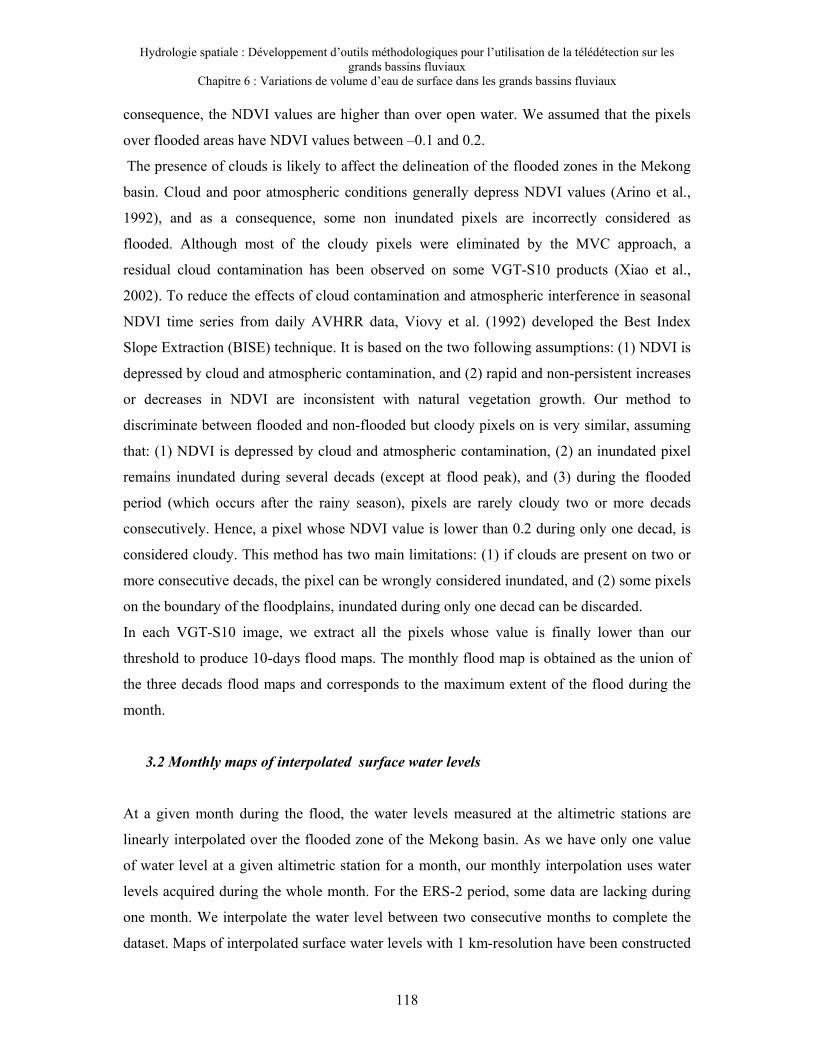
Hydrologie spatiale : Développement d’outils méthodologiques pour l’utilisation de la télédétection sur les grands bassins fluviaux
Chapitre 6 : Variations de volume d’eau de surface dans les grands bassins fluviaux
118
consequence, the NDVI values are higher than over open water. We assumed that the pixels
over flooded areas have NDVI values between –0.1 and 0.2.
The presence of clouds is likely to affect the delineation of the flooded zones in the Mekong
basin. Cloud and poor atmospheric conditions generally depress NDVI values (Arino et al.,
1992), and as a consequence, some non inundated pixels are incorrectly considered as
flooded. Although most of the cloudy pixels were eliminated by the MVC approach, a
residual cloud contamination has been observed on some VGT-S10 products (Xiao et al.,
2002). To reduce the effects of cloud contamination and atmospheric interference in seasonal
NDVI time series from daily AVHRR data, Viovy et al. (1992) developed the Best Index
Slope Extraction (BISE) technique. It is based on the two following assumptions: (1) NDVI is
depressed by cloud and atmospheric contamination, and (2) rapid and non-persistent increases
or decreases in NDVI are inconsistent with natural vegetation growth. Our method to
discriminate between flooded and non-flooded but cloody pixels on is very similar, assuming
that: (1) NDVI is depressed by cloud and atmospheric contamination, (2) an inundated pixel
remains inundated during several decads (except at flood peak), and (3) during the flooded
period (which occurs after the rainy season), pixels are rarely cloudy two or more decads
consecutively. Hence, a pixel whose NDVI value is lower than 0.2 during only one decad, is
considered cloudy. This method has two main limitations: (1) if clouds are present on two or
more consecutive decads, the pixel can be wrongly considered inundated, and (2) some pixels
on the boundary of the floodplains, inundated during only one decad can be discarded.
In each VGT-S10 image, we extract all the pixels whose value is finally lower than our
threshold to produce 10-days flood maps. The monthly flood map is obtained as the union of
the three decads flood maps and corresponds to the maximum extent of the flood during the
month.
3.2 Monthly maps of interpolated surface water levels
At a given month during the flood, the water levels measured at the altimetric stations are
linearly interpolated over the flooded zone of the Mekong basin. As we have only one value
of water level at a given altimetric station for a month, our monthly interpolation uses water
levels acquired during the whole month. For the ERS-2 period, some data are lacking during
one month. We interpolate the water level between two consecutive months to complete the
dataset. Maps of interpolated surface water levels with 1 km-resolution have been constructed

Hydrologie spatiale : Développement d’outils méthodologiques pour l’utilisation de la télédétection sur les grands bassins fluviaux
Chapitre 6 : Variations de volume d’eau de surface dans les grands bassins fluviaux
119
for each month, between July and December, for the 1998-2003 period. ERS-2-derived
surface water levels are used in the interpolation process for the period 1998-2002 and
ENVISAT RA-2 for 2003. As mentioned above, water levels are expressed with respect to
the geoid. For the purpose of hydrological interpretation of water volumes, referring to the
topography would be best as far as floodplains are concerned. However, available topographic
data bases are not necessarily precise enough for the present study. As a consequence of using
the geoid as reference, only month to month difference maps really represent water volume
change (see below).
Over the western/eastern flowing parts of the river network, the ERS-2/ENVISAT tracks
cross the river and its floodplain system, allowing to define several altimetric stations over the
river mainstream and associated floodplains (see Fig.3). As a consequence, the interpolation
in the along-track direction follows the difference of water levels between the mainstream and
the floodplain. In the cross-track direction, interpolation over several tenths of kilometers will
only reflect the mean slope of the river. Over the northern/southern flowing parts of the river
network, the ERS-2/ENVISAT tracks run along strike the river. In these cases, depending on
the choice of the geographical coordinates of the altimetric station, the time series can be
influenced by the variation of level within the adjacent floodplain (Birkett et al., 2002). These
authors did not report obvious amplitude or phase differences due to the inclusion of some
floodplain. On the central floodplain, the network of altimetric stations is sufficiently dense to
avoid important errors of interpolation.
The monthly flood maps indicate that the flood period generally ranges from September to
November. As an example for year 2003, Fig.7 shows maps of interpolated water levels
between July and December 2003. The monthly flood maps indicate that the flood period
generally ranges from September to November In July and August, no flood is observed in the
Mekong basin. In September, the upstream part of the Mekong basin is flooded. Water levels
decrease in the upstream part of the Mekong river whereas they still rise in the Tonle Sap
river between September and October. This situation corresponds to the reversal flow of the
Tonle Sap River: during the flood, the water flows from the Mekong River to the Tonle Sap
River whereas it flows from the Tonle Sap to the Mekong River when the water level
decreases. The flood reaches the delta in October. The level of the Tonle Sap river decreases
between November and October and the downstream part of the basin is inundated in
November. The flood has ended in December, the situation is similar to month of July. Fig.8
presents maps of water level differences for two couples of consecutive months (October

Hydrologie spatiale : Développement d’outils méthodologiques pour l’utilisation de la télédétection sur les grands bassins fluviaux
Chapitre 6 : Variations de volume d’eau de surface dans les grands bassins fluviaux
120
minus September 2003) and (November minus October 2003). Note that this figure represents
a ‘real’ water volume quantity. The sequence of events discussed above are even more visible
in Fig.9.
Important variations in the extent of the flooded zone can be observed from one year to
another. This is illustrated in Fig.9 which shows maps interpolated water levels for the month
of October over 1998-2003. Year 2000 is characterized by an exceptionally long flood period,
from August to December. The maximum extent is reached in 2000, and years 2001 and
2002 present large floods compared with years 1998, 1999 and 2003.
4. Water volume variations
4.1 surface water volume change
Determining the temporal variation of water volume stored in the floodplains has many
applications in hydrology. For the inundated areas permanently or temporarily connected to
main channels, the determination of the water volume variation is equivalent to the estimation
of water volume potentially stored and/or released by the valley reach during flood stages.
The water volume variation in this type of inundated areas is an important parameter for the
hydrodynamic modelling of the river flow and the determination of its transport capacity. For
the inundated areas that never connect to the main channel, the volume variation is essentially
a function of the base flow variation, the inputs from the local basin and the rain. Some
floodplains present both types of flooding zones. Areas where the river water mixes with the
local water are called “perirheic zones” (Mertes, 1997). In all cases, the inundation area is a
buffer zone between the river and the upland watershed. The water volume variation
represents the flood pulse of floodplains as expressed by Junk et al. (1989). Therefore, it is a
key ecological characteristic that cannot be easily measured in the field.
The variation of water volume corresponds to the surface water levels difference integrated
over the inundated surface. These variations δV(ti,ti-1), between two consecutive months
numbered i and i-1, over the floodplain S is the sum of the products of the difference of
surface water levels δhj(i,i-1), with j=1, 2, … inside S, by the elementary surfaces Re2 δλ δθ
sinθj :
)sin()1,,,()1,( 2j
Sj
je iihRiiV θλθδδλδθδ ∑∈ −=− (2)

Hydrologie spatiale : Développement d’outils méthodologiques pour l’utilisation de la télédétection sur les grands bassins fluviaux
Chapitre 6 : Variations de volume d’eau de surface dans les grands bassins fluviaux
121
where δλ and δθ are the sampling grid steps along longitude and latitude (~0.01°),
respectively and Re the mean radius of the Earth (~6378 km). The surface water volume
variations are expressed in km3/month.
Figure 10 presents the differences between two consecutive months of the mean water volume
averaged over the study area for 1996-2003. Only months from August to December are
considered. Positive variations are obtained between August and October. They are more
important for the years 2000, 2001, 2002 than for 1998, 1999 and 2003, with volume
variations greater than 15 km3 and reaching 25 km3 between September and August 2002. The
important flood of 2000 can be related to the exceptional precipitation event. No similar
events can be invoked to explain the great floods of 2001 and 2002.
4.2 comparison with the total water volume change determined by GRACE.
The GRACE mission, launched in March 2002, is devoted to measure spatio-temporal change
of the gravity that results mainly from water mass redistribution among the surface fluid
envelops (Tapley et al., 2004a). Several recent studies have shown that GRACE data over the
continents provide important new information on the total land water storage (surface waters,
soil moisture and underground waters, and where appropriate on snow mass) (Tapley et al.,
2004b, Wahr et al., 2004, Chen et al., 2005, Schmidt et al., 2005, Ramillien et al., 2005).
Ramillien et al. (2005) computed monthly change in total water mass volume in several
different river basins, including the Mekong. On Fig. 10 is presented the differences between
two consecutive months of the vertically integrated water volume change from GRACE over
the whole Mekong basin for the period May 2002 – April 2004. Comparing with monthly
differences in surface water volume change computed in the present study, we note that the
GRACE-derived total water volume differences display almost in phase seasonal fluctuations.
The agreement is particularly good during periods of water falling and around minimum water
level. It should be recalled however that GRACE provides the sum of surface waters and
soil/underground waters. In addition, due to the current GRACE spatial resolution (~ 600
km), the land water storage has been computed over the whole Mekong basin, an area much
larger than that considered in the present study. However this comparison shows that in the
future when the GRACE resolution will improve, it could be possible to combine the GRACE

Hydrologie spatiale : Développement d’outils méthodologiques pour l’utilisation de la télédétection sur les grands bassins fluviaux
Chapitre 6 : Variations de volume d’eau de surface dans les grands bassins fluviaux
122
result with the water volume change inferred from altimetry data to extract the subsurface
water storage change.
5. Conclusion
This study showed that combining altimetry-based water levels with satellite imagery (here
NDVI data from the SPOT/Vegetation instrument) provides a new method for remotely
measure surface water volumes over large floodplains. It also showed that the rather dense
coverage of ERS/ENVISAT satellites (compared to Topex/Poseidon) over the Mekong
floodplains allows to describe the geographical variations in seasonal high/low water levels.
In particular we noticed a strong difference between the northern part of the Lower Mekong
(upstream of the intersection between the main river and the Tonle Sap river, as well as the
Tonle Sap region) and the southern part which includes the main floodplain and delta. The
latter shows very small seasonal fluctuations (less than 2 m) compared to the former (up to 10
m). This may possibly results from the many canals and dams built during the last two
decades in the floodplain area.

Hydrologie spatiale : Développement d’outils méthodologiques pour l’utilisation de la télédétection sur les grands bassins fluviaux
Chapitre 6 : Variations de volume d’eau de surface dans les grands bassins fluviaux
123
Figure Caption
Figure 1: Map of the Mekong basin.
Figure 2: Mode 1 of the EOF decomposition of precipitation (GPCC) over the lower Mekong,
between 1996 and 2003.
Figure 3: Spatial coverage of radar altimeters over the Mekong basin. The red lines
correspond to ERS-2/ENVISAT tracks, the yellow dotted lines correspond to T/P tracks. The
80 virtual stations are represented using white dots, the yellow stars correspond to the ones
presented on figure 5. The white circle correspond to the intersection between T/P and ERS-
2/ENVISAT tracks.
Figure 4: Comparison between T/P and ERS-2/ENVISAT derived water level time-series.
Figure 5: Examples of time-series of water level derived from ERS-2 in the lower Mekong
basin.
Figure 2: Mode 1 of the EOF decomposition of water levels derived from radar altimetry over
the lower Mekong, between 1996 and 2003.
Figure 7: Water level maps (wrt GRACE geoid) from July to December 2003.
Figure 8: Water level difference maps: October minus September 2003 and November minus
October 2003.
Figure 9: Water level maps (wrt GRACE geoid) for October 1998 to 2003.
Figure 10: Variation of water volume for the surface water (green) and the total land waters
(black).

Hydrologie spatiale : Développement d’outils méthodologiques pour l’utilisation de la télédétection sur les grands bassins fluviaux
Chapitre 6 : Variations de volume d’eau de surface dans les grands bassins fluviaux
124
References
AVISO (1996). AVISO User Handbook: Merged TOPEX/POSEIDON Products, AVI-NT-02-
101-CN, 3-rd ed, CNES, Toulouse, France, 194 pp.
Arino O., Dedieu G., Deschamps P. (1992). Determination of satellite land surface
reflectances using METEOSAT and NOAA/AVHRR shortwave channel data, Int. J. Remote
Sensing, 13, 2263-2287.
Arnaud M., Leroy M.,M. (1991). SPOT 4: a new generation of SPOT satellites, ISPRS
Journal of Photogrammetry and Remote Sensing, 46, 205-215.
Bamber J.L. (1994). Ice sheet altimeter processing scheme, Int. J. Remote Sensing, 15 (4),
925-938.
Birkett C.M. (1998). Contribution of the TOPEX NASA radar altimeter to the global
monitoring of large rivers and wetlands, Water Resour. Res., 34 (5), 1223-1239.
Birkett C.M., Mertes L.A.K., Dunne T., Costa M.H., Jasinski M.J. (2002). Surface water
dynamics in the Amazon Basin : Application of satellite radar altimetry, J. Geophys. Res., 107
(D20), 8059-8080.
Chen et al., 2005
Chia A.S., Chen P., Liew S.C. (2001). Flood extent in the Lower Mekong Basin evaluated
using SPOT Quicklook mosaics, 22nd
Asian Conference on Remote Sensing, 5-9 November
2001.
Dow J.M., Martinez Fadrique F.M., Zandbergen R. (1999). High precision altimetry from the
ENVISAT mission, Adv. Space Res., 23 (4), 757-762.

Hydrologie spatiale : Développement d’outils méthodologiques pour l’utilisation de la télédétection sur les grands bassins fluviaux
Chapitre 6 : Variations de volume d’eau de surface dans les grands bassins fluviaux
125
Duchemin B., Berthelot B., Dedieu G., Leroy M., Maisongrande P. (2002). Normalisation of
directional effects in 10-day global syntheses derived from VEGETATION/SPOT : II.
Validation of an operational method on actual datasets, Remote Sens. Env., 81, 101-113.
ESA (2002). ENVISAT RA2/MWR Product Handbook, RA2 /MWR Products User Guide.
Frappart F., Seyler F., Martinez J.M., Leỏn J.G., Cazenave A. (in press a). Floodplain Water
Storage in the Negro River Basin Estimated from Microwave Remote Sensing of Inundation
Area and Water Levels, Remote Sens. Env.
Frappart F., Cazenave A., Seyler F., Calmant S. (in press b). Preliminary results of ENVISAT
RA-2 Derived Water Levels Validation over the Amazon Basin., Remote Sens. Env.
Gardini B., Graf G., Ratier G. (1995). The instruments on ENVISAT, Acta Astronautica, 37,
301-311.
Hoanh C.T., Guttman H., Droogers, Aerts J. (2003). Water, climate, food, and environment is
the Mekong basin in southeast Asia, Contribution to project ADAT, Adaptation strategies to
changing environments, Final report, 58 pp.
Holben B.N. (1986). Characteristics of maximum-value composite images from temporal
AVHRR data, Int. J. Remote Sensing, 7, 1417-1434.
Hori H. (2000). The Mekong environment and development, the United Nations University,
New York USA.
IMC (1988). Perspectives for Mekong Development. Revised indicative plan (1987) for the
development of land, water and related resources of the lower Mekong basin. Committee
report. Interim Committee for Coordination of Investigations of the lower Mekong Basin,
Bangkok, Thailand.
Hydrologie spatiale : Développement d’outils méthodologiques pour l’utilisation de la télédétection sur les grands bassins fluviaux
Chapitre 6 : Variations de volume d’eau de surface dans les grands bassins fluviaux
126
Junk W., Bayley P.B., Sparks R.E, 1989. The flood pulse concept in river floodplain systems,
in D.P. Dodge (Ed.) Proceedings of the International Large River Symposium. Can. Spec.
Pub. Fish. Aquat. Sci. 106, 110-127.
Laxon S. (1994). Sea ice altimeter processing scheme at the EODC, Int. J. Remote Sensing, 15
(4), 915-924.
Legrésy B. (1995). Etude du retracking des surfaces des formes d’onde altimétriques au-
dessus des calottes, rapport CNES, CT/ED/TU/UD96.188, contrat n° 856/2/95/CNES/006, 81
pp.
Maheu C., Cazenave A., Mechoso C. R. (2003). Water level fluctuations in the Plata basin
(South America) from Topex/Poseidon satellite altimetry, Geophys. Res. Let., 30 (3), 1143-
1146.
Mertes L.A.K. (1997). Documentation and significance of the perirheic zone on inundated
floodplains. Water Resour. Res., 33 ( 7), 1749-1762.
MRC and UNEP (1997). Mekong River Basin diagnostic study. Final report. Mekong River
Commission (MRC), Pnomh Penh, Cambodia.
MRC (2002).Annual report. Mekong River Commission (MRC) Secretariat, Pnomh Penh,
Cambodia.
Ramillien G., Frappart F., Cazenave A., Güntner A. (2005). Time variations of the land water
storage from an inversion of 2 years of GRACE geoids, Earth Planet. Sci. Lett., 235, 283-301.
Reigber C., Schmidt R., Flechtner F., König R., Meyer U., Neumayer K.H., Schwintzer P.,
Zhu S.Y. (2005). An Earth gravity field model complete to degree and order 150 from
GRACE: EIGEN-GRACE02S, Journal of Geodynamics, 39 (1), 1-10.

Hydrologie spatiale : Développement d’outils méthodologiques pour l’utilisation de la télédétection sur les grands bassins fluviaux
Chapitre 6 : Variations de volume d’eau de surface dans les grands bassins fluviaux
127
Rudolf, B., Hauschild H., Rueth W., Schneider U. (1994). Terrestrial Precipitation Analysis:
Operational Method and Required Density of Point Measurements. In: Global Precipitations
and Climate Change (Ed. M. Desbois, F. Desalmond), NATO ASI Series I, Vol. 26, Springer-
Verlag, p. 173-186.
Rudolf, B., Fuchs T., Schneider U., Meyer-Christoffer A. (2003). Introduction of the Global
Precipitation Climatology Centre (GPCC), Deutscher Wetterdienst, Offenbach a.M.; pp. 16.
Schmidt R., Flechtner F., Reigber C., Schwintzer P., Güntner A., Döll P., Ramillien G.,
Cazenave A., Petrovic S., Jochman H., Wunsch J. (2005). GRACE observations of changes in
continental water storage, Glob. And Plan. Change, in press.
Tapley B.D., Bettadpur S., Watkins M., Reigber C. (2004a). The Gravity Recovery and
Climate Experiment : Mission overview and Early results, Geophys. Res. Lett., 31, L09607,
doi:10.1029/2004GL019920.
Tapley B.D., Bettadpur S., Ries J.C., Thompson P.F Watkins M. (2004b). GRACE
measurements of mass variability in the Earth system, Science, 305, 503-505.
Toumazou V., Crétaux J.F. (2001). “Using a Lanczos eigensolver in the computation of
Empirical Orthogonal Functions, Monthly Weather Review, 129(5), 1243-1250, doi:
10.1175/1520-0493.
Tucker C.J. (1979). Red and photographic infrared linear combinations for monitoring
vegetation, Remote Sens. Env., 8, 127-150.
Viovy N., Arino O., Belward A.S. (1992). The Best Index Slope Extraction (BISE): A method
for reducing noise in NDVI time-series, Int. J. Remote Sensing, 13 (8), 1585-1590.
Wahr J., Molenaar M., Bryan F. (1998). Time-variability of the Earth’s gravity field:
hydrological and oceanic effects and their possible detection using GRACE, J. Geophys. Res.,
103, 30, 205-30,230.

Hydrologie spatiale : Développement d’outils méthodologiques pour l’utilisation de la télédétection sur les grands bassins fluviaux
Chapitre 6 : Variations de volume d’eau de surface dans les grands bassins fluviaux
128
Wahr et al., 2004
Wehr T., Attema E. (2001). Geophysical validation of ENVISAT data products, Adv. Space
Res., 28 (1), 83-91.
Wingham D.J., Rapley C.G., Griffiths H. (1986). New techniques in satellite altimeter
tracking systems, Proceedings of IGARSS’86 Symposium, Zürich, 8-11 Sept. 1986, Ref. ESA
SP-254, 1339-1344.
Xiao X., Boles S., Liu J., Zhuang D., Liu M. (2002). Characterization of forest type in
northeastern China, using multi-temporal SPOT-4 VEGETATION sensor data, Remote Sens.
Env., 82, 335-348.
Zelli C. (1999). ENVISAT RA-2 advanced radar altimeter : Instrument design and pre-launch
performance assessment review, Acta Astronautica, 44, 323-333.

Hydrologie spatiale : Développement d’outils méthodologiques pour l’utilisation de la télédétection sur les grands bassins fluviaux
Chapitre 6 : Variations de volume d’eau de surface dans les grands bassins fluviaux
129
Fig.1

Hydrologie spatiale : Développement d’outils méthodologiques pour l’utilisation de la télédétection sur les grands bassins fluviaux
Chapitre 6 : Variations de volume d’eau de surface dans les grands bassins fluviaux
130
Fig.2

Hydrologie spatiale : Développement d’outils méthodologiques pour l’utilisation de la télédétection sur les grands bassins fluviaux
Chapitre 6 : Variations de volume d’eau de surface dans les grands bassins fluviaux
131
Fig.3

Hydrologie spatiale : Développement d’outils méthodologiques pour l’utilisation de la télédétection sur les grands bassins fluviaux
Chapitre 6 : Variations de volume d’eau de surface dans les grands bassins fluviaux
132
Fig.4
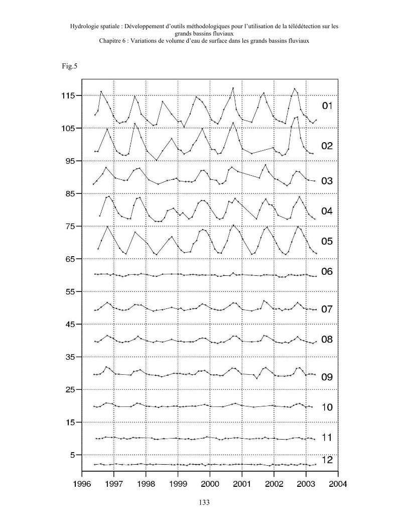
Hydrologie spatiale : Développement d’outils méthodologiques pour l’utilisation de la télédétection sur les grands bassins fluviaux
Chapitre 6 : Variations de volume d’eau de surface dans les grands bassins fluviaux
133
Fig.5

Hydrologie spatiale : Développement d’outils méthodologiques pour l’utilisation de la télédétection sur les grands bassins fluviaux
Chapitre 6 : Variations de volume d’eau de surface dans les grands bassins fluviaux
134
Fig.6

Hydrologie spatiale : Développement d’outils méthodologiques pour l’utilisation de la télédétection sur les grands bassins fluviaux
Chapitre 6 : Variations de volume d’eau de surface dans les grands bassins fluviaux
135
Fig.7
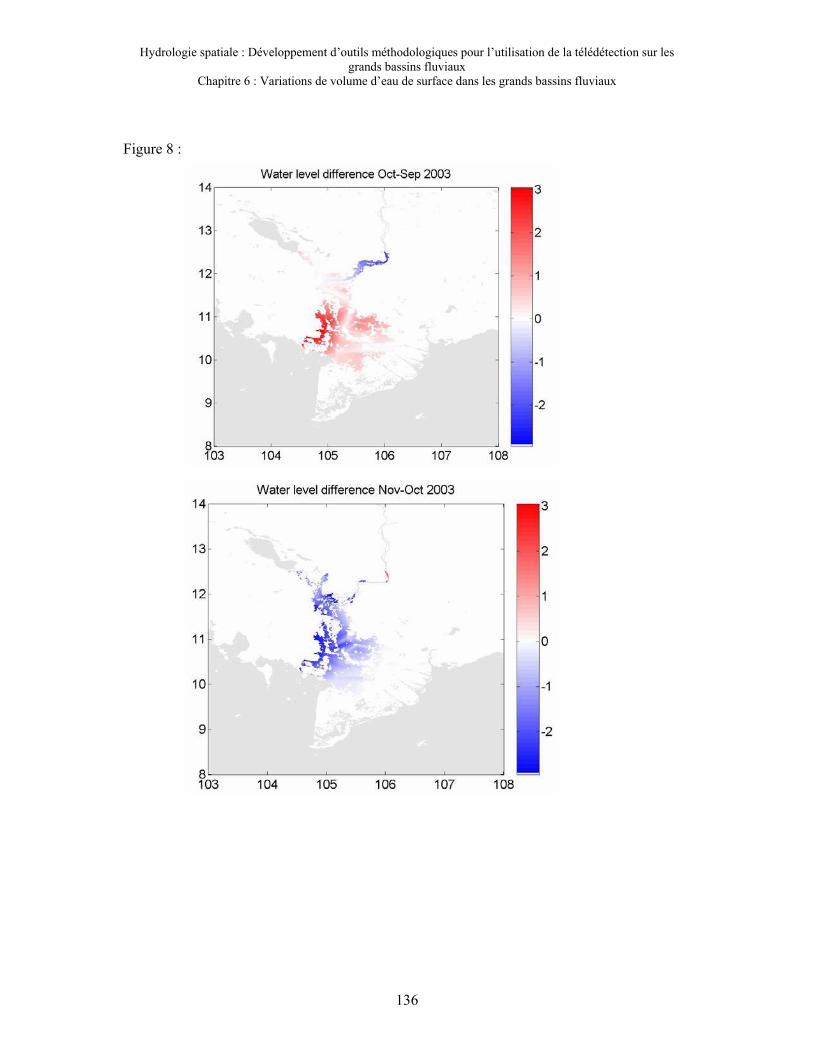
Hydrologie spatiale : Développement d’outils méthodologiques pour l’utilisation de la télédétection sur les grands bassins fluviaux
Chapitre 6 : Variations de volume d’eau de surface dans les grands bassins fluviaux
136
Figure 8 :

Hydrologie spatiale : Développement d’outils méthodologiques pour l’utilisation de la télédétection sur les grands bassins fluviaux
Chapitre 6 : Variations de volume d’eau de surface dans les grands bassins fluviaux
137
Figure 9 :

Hydrologie spatiale : Développement d’outils méthodologiques pour l’utilisation de la télédétection sur les grands bassins fluviaux
Chapitre 6 : Variations de volume d’eau de surface dans les grands bassins fluviaux
138
Figure 10 :

Hydrologie spatiale : Développement d’outils méthodologiques pour l’utilisation de la télédétection sur les grands bassins fluviaux
Chapitre 6 : Variations de volume d’eau de surface dans les grands bassins fluviaux
139
4. Conclusion
Ces deux études mettent en évidence que la combinaison de niveaux d’eau déduits des
mesures altimétriques et de l’imagerie permet de calculer des variations de volume d’eau
stocké dans les plaines d’inondation des grands bassins fluviaux. La comparaison entre
volume stocké et volume écoulé (quand des mesures de débit sont disponibles) est un
indicateur du temps de résidence de l’eau dans les plaines d’inondation.
Cette nouvelle méthode permet de caractériser le changement dans le cycle hydrologique des
fleuves sous l’effet de modifications des conditions climatiques ou des activités humaines
(construction de barrage, de canaux d’irrigation, déforestation…).
Cette méthode présente de quatre limites importantes : tout d’abord, elle ne permet de calculer
le volume d’eau présent dans le bassin à une date donnée, seules les variations entre deux
dates sont disponibles. Seul le développement de modèles numériques de terrain de grande
précision, à l’échelle du bassin versant donneront accès aux stocks d’eau.
La deuxième limitation concerne la couverture spatiale et la répétitivité temporelle des
altimètres actuellement en fonctionnement sur les grands bassins versants qui est encore
insuffisante. T/P donne accès à des niveaux d’eau tous les 10 jours, mais l’intertrace à
l’équateur est de 315 km. Pour ERS et ENVISAT, l’inverse se produit : résolution spatiale
dense mais faible répétitivité temporelle.
Le troisième point est lié à la nature des images utilisées : si les données SAR, permettant
d’avoir accès à l’eau sous végétation, ont une très faible répétitivité temporelle, les images
multispectrales, à forte répétitivité temporelle, présentent l’inconvénient de ne pas être
utilisables dans des régions où les couverts végétal ou nuageux est important.
Il n’existe enfin aucune source de données in-situ pouvant être utilisée à des fins de
validation.

Hydrologie spatiale : Développement d’outils méthodologiques pour l’utilisation de la télédétection sur les grands bassins fluviaux
Chapitre 6 : Variations de volume d’eau de surface dans les grands bassins fluviaux
140

Hydrologie spatiale : Développement d’outils méthodologiques pour l’utilisation de la télédétection sur les
grands bassins fluviaux
Chapitre 7 : GRACE et l’hydrologie continentale
141
Chapitre 7 : GRACE et l’hydrologie continentale
Chapitre 7 : GRACE et l’hydrologie continentale ................................................................. 141 1. Le bilan hydrique du bassin versant........................................................................................................... 142 2. Les modèles hydrologiques globaux.......................................................................................................... 143
2.1 Le modèle WGHM............................................................................................................................. 144 2.2 Le modèle LaD................................................................................................................................... 144 2.3 Le modèle ORCHIDEE...................................................................................................................... 144 2.4 Le système d’assimilation GLDAS ................................................................................................... 144
3. La mission de gravimétrie spatiale GRACE.............................................................................................. 145 3.1 Les objectifs........................................................................................................................................ 145 3.2 Les géoïdes mensuels ......................................................................................................................... 146
4. Application à l’hydrologie globale ............................................................................................................ 147 4.1 Travaux antérieurs.............................................................................................................................. 148 4.2 Méthodologie...................................................................................................................................... 148
5. Résultats...................................................................................................................................................... 149 5.1 Validation de la méthode inverse....................................................................................................... 149 5.2 Estimation des masses d’eaux continentales ..................................................................................... 169 5.3 Estimation des masses de neige aux latitudes boréales..................................................................... 173 5.4 Estimation de l’évapotranspiration à l’échelle du basin versant ....................................................... 179
6. Discussion – Perspectives .......................................................................................................................... 196

Hydrologie spatiale : Développement d’outils méthodologiques pour l’utilisation de la télédétection sur les
grands bassins fluviaux
Chapitre 7 : GRACE et l’hydrologie continentale
142
1. Le bilan hydrique du bassin versant
L’humidité des sols, les nappes phréatiques, la neige, la glace, les lacs et rivières, l’eau
contenue dans la végétation sont les réservoirs principaux dans lesquels l’eau est présente sur
les continents. Bien qu’ils ne constituent que 3,5% de l’eau du cycle hydrologique, leur
influence sur le climat et sur la vie sur terre est considérable [Chahine, 1992 ; Rodell et
Famiglietti, 1999 ; de Marsily, 2005].
La quantification des volumes d’eau dans les différents compartiments du cycle hydrologique,
à toute échelle de temps et d’espace, est l’une des interrogations majeures posées aux
hydrologues. Les bilans en hydrologie ont été définis pour permettre d’estimer la répartition
de l’eau qui tombe sous forme de précipitation, entre évaporation et ruissellement [Cosandey
et Robinson, 2000]. Le bilan hydrique fait intervenir les flux d’eau entrants et sortants du
bassin versant (Figure 7-1).
Il peut s’exprimer de la façon suivante, pour un bassin et un intervalle de temps donnés :
REPV −−=∆ (Eq. 7-1)
Figure 7-1: Le bilan hydrique à l'échelle du bassin versant.

Hydrologie spatiale : Développement d’outils méthodologiques pour l’utilisation de la télédétection sur les
grands bassins fluviaux
Chapitre 7 : GRACE et l’hydrologie continentale
143
où ∆V est la variation de volume d’eau (mm), P la somme des précipitations liquides et
solides (mm), R la somme du ruissellement de surface et des écoulements souterrains (mm).
Les termes du bilan hydrique sont généralement exprimés en hauteur équivalente d'eau (en
mm par exemple). On parle alors de lame d'eau précipitée, écoulée, évaporée, stockée, ...
Cette équation exprime simplement que la différence entre les volumes d'eau entrant et sortant
d'une entité donnée, comme un bassin versant, au cours de la période considérée, est égale à la
variation du volume d'eau emmagasinée au cours de la dite période.
Avant le lancement de la mission de gravimétrie spatiale GRACE (Gravity Recovery And
Climate Experiment), seules les sortie des modèles globaux de surface étaient en mesure de
fournir des estimations des réserves mondiales en eau et de leurs variations, et permettaient de
calculer le bilan hydrique à l’échelle du bassin versant ou globale [Wahr et al. 1998 ; Swenson
et al., 2003 ; Ilk et al., 2005].
2. Les modèles hydrologiques globaux
Il n’existe, en effet, à l’heure actuelle, aucune base de données in-situ, à l’échelle du globe,
permettant de quantifier les variations spatio-temporelles des réserves continentales d'eau
(eau des sols, des réservoirs souterrains et du manteau neigeux). Seuls les modèles globaux de
surface, développés ces dernières années par la communauté des hydrologues-climatologues,
nous renseignent sur ces paramètres. Ses modèles représentent le sol comme une succession
de réservoirs, ou couches, superposés : humidité des sols, eaux de surface, zone racinaire,
aquifères. Le rôle de la végétation (interception des précipitations et transpiration) est
désormais pris en compte. Les processus spécifiques à la cryosphère, comme l’accumulation
et la fonte de la neige ou le cycle gel/dégel des sols sont également modélisés. Une
description complète du cycle du carbone et de la dynamique de la végétation a été introduite
pour les études sur les changements climatiques. Enfin, des modèles de transport fluviaux ont
été développés pour router le ruissellement de chaque point de grille vers l’embouchure des
fleuves. Ces schémas de surface sont soit forcés par des flux observés (précipitation et bilan
radiatif) et des variables météorologiques à l’interface sol-atmosphère (température, humidité
de l’air, intensité et direction des vents), soit couplés à des modèles atmosphériques.
Dans le cadre de la validation des mesures de la mission GRACE, nous nous sommes
intéressés aux sorties de trois schémas de surface globaux, WGHM (Water GAP Global
Hydrology Model) [Döll et al., 2003], LaD (Land Dynamics model) [Milly and Shmakin,
2002], ORCHIDEE (ORganising Carbon and Hydrology In Dynamic EcosystEms) [Verant et

Hydrologie spatiale : Développement d’outils méthodologiques pour l’utilisation de la télédétection sur les
grands bassins fluviaux
Chapitre 7 : GRACE et l’hydrologie continentale
144
al., 2004 ; Krinner et al., 2005], et du schéma d’assimilation GLDAS (Global Land Data
Assimilation System) [Rodell et al., 2004].
2.1 Le modèle WGHM
Le modèle WGHM, développé par [Döll et al., 2003], a été spécifiquement conçu pour
évaluer le débit des fleuves dans le cadre d’études d’estimation des ressources en eau. Il
calcule des cartes mensuelles de ruissellement à la résolution spatiale de 0,5° et le débit des
fleuves au moyen d’un schéma de routage. Sa paramétrisation a été effectuée en utilisant des
séries temporelles de débit mesurées par 724 stations hydrologiques disséminées sur le globe.
Ses sorties mensuelles comprennent d’autres paramètres hydrologiques comme l’humidité du
sol contenue dans la zone racinaire, les aquifères, les eaux de surface (fleuves, lacs, plaines
d’inondation), l’épaisseur de neige, l’évapotranspiration. Les données utilisées couvrent la
période 2002-2004.
2.2 Le modèle LaD
Le modèle LaD, développé par [Milly and Shmakin, 2002], est un modèle de surface simple
comportant quatre réservoirs : zone racinaire, eaux du sol, neige, glace. Il fournit des cartes
d’humidité du sol, d’eau du sol correspondant à une zone située entre 1 et 2 m de profondeur,
d’épaisseur de neige, d’évapotranspiration, à la résolution de 1°, de 1981 à 2004.
2.3 Le modèle ORCHIDEE
Le modèle ORCHIDEE décrit les cycles de l’eau et du carbone à l’interface sol-plantes-
atmosphère, ainsi que l’évolution de la végétation. Il est le résultat du couplage de 3 modèles
existants : SECHIBA (Schématisation des Echanges Hydriques à l’Interface Biosphère-
Atmosphère) [Ducoudré et al., 1993], qui simule les processus physiques à l’interface sol-
végétation-atmosphère et les flux d’eau dans le sol, STOMATE (Saclay Toulouse Orsay
Model for the Analysis of Terretrial Ecosystems) [Viovy, 1996], qui décrit les processus
biochimiques en surface, et LPJ (Lund Postdam Jena) [Sitch et al., 2000], qui reproduit
l’évolution de la végétation et le bilan de carbone. Il fournit des cartes mensuelles de
paramètres de surface, à la résolution de 1°, pendant la période 1948-2003.
2.4 Le système d’assimilation GLDAS
Ce modèle non couplé à l’atmosphère, utilisé pour des études sur le climat, est forcé en temps
réel par des champs provenant des ré-analyses du modèle météorologique NCEP, de mesures

Hydrologie spatiale : Développement d’outils méthodologiques pour l’utilisation de la télédétection sur les
grands bassins fluviaux
Chapitre 7 : GRACE et l’hydrologie continentale
145
satellitaires et de données radar de précipitation. L’assimilation de données, comme la
température de surface ou le couvert neigeux, par filtrage de Kalman à une dimension, permet
d’estimer de manière optimale les valeurs des paramètres de surface. Les résolutions spatiale
et temporelle des grilles de paramètres de surface sont de 0,25° et 3 heures. Les données sont
disponibles pour la période 2002-2004.
3. La mission de gravimétrie spatiale GRACE
Les changements temporels du champ de gravité terrestre, détectés par la mission de
gravimétrie spatiale GRACE, caractérisent les redistributions de masse dans le système Terre.
Aux échelles de temps allant d’un mois à quelques années, ces redistributions proviennent des
variations des réserves continentales d’eau. L’un des principaux objectifs de cette mission
satellitaire est d’estimer les variations spatio-temporelles du stock continental d’eau à
l’échelle du globe. La détermination de ces variations a pour but de fermer le bilan hydrique
des grands bassins fluviaux et des continents, et de servir à la validation et à l’amélioration
des modèles hydrologiques existants, afin de décrire plus précisément le cycle hydrologique et
les impacts des changements climatiques et environnementaux [Ilk et al., 2005].
3.1 Les objectifs
La mission Gravity Recovery And Climate Experiment (GRACE), lancée en mars 2002 pour
une durée de vie de 5 ans, été conçue, par la NASA et le DLR, pour observer les variations du
champ de gravité terrestre [Watkins et Bettadpur, 2000 ; Tapley et Reigber, 2001]. Elle a pour
but de cartographier, chaque mois, le champ de gravité à une résolution spatiale de 400 km
[Tapley et al., 2004 a]. Elle se compose de deux satellites identiques, suivant une orbite quasi
circulaire, à 500 km d’altitude et une inclinaison de 89,5°, séparés l’un de l’autre par une
distance de l’ordre de 220 kilomètres. Un système de télémétrie micro-onde (en bande K)
mesure de manière précise la distance séparant les deux satellites. En outre, chaque satellite
embarque un récepteur GPS et des capteurs d’attitude [Dunn et al., 2003], ainsi qu’un
accéléromètre pour mesurer, avec précision, les effets des forces non gravitationnelles que
sont la pression solaire, le frottement atmosphérique et d’autres phénomènes non modélisés
[Touboul et al., 1999].
Pour obtenir une erreur inférieure à 2 cm sur les modèles de géoïde [Ward et al., 2002], les
mesures du déphasage réalisés par le système de télémétrie, sont traitées au sol. Les effets des
forces non-gravitationnelles, mesurés par les accéléromètres, sont retirés du signal observé
pour obtenir la composante purement gravitationnelle, liée à la distribution de masse à
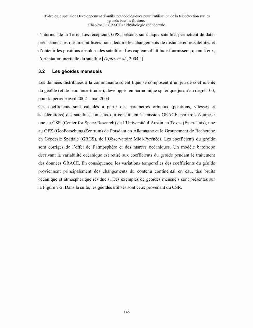
Hydrologie spatiale : Développement d’outils méthodologiques pour l’utilisation de la télédétection sur les
grands bassins fluviaux
Chapitre 7 : GRACE et l’hydrologie continentale
146
l’intérieur de la Terre. Les récepteurs GPS, présents sur chaque satellite, permettent de dater
précisément les mesures utilisées pour déduire les changements de distance entre satellites et
d’obtenir les positions absolues des satellites. Les capteurs d’attitude fournissent, quant à eux,
l’orientation inertielle du satellite [Tapley et al., 2004 a].
3.2 Les géoïdes mensuels
Les données distribuées à la communauté scientifique se composent d’un jeu de coefficients
du géoïde (et de leurs incertitudes), développés en harmonique sphérique jusqu’au degré 100,
pour la période avril 2002 – mai 2004.
Ces coefficients sont calculés à partir des paramètres orbitaux (positions, vitesses et
accélérations) des satellites jumeaux qui constituent la mission GRACE, par trois équipes :
une au CSR (Center for Space Research) de l’Université d’Austin au Texas (Etats-Unis), une
au GFZ (GeoForschungsZentrum) de Potsdam en Allemagne et le Groupement de Recherche
en Géodésie Spatiale (GRGS), de l’Observatoire Midi-Pyrénées. Les coefficients du géoïde
sont corrigés de l’effet de l’atmosphère et des marées océaniques. Un modèle barotrope
décrivant la variabilité océanique est retiré aux coefficients du géoïde pendant le traitement
des données GRACE. En conséquence, les variations temporelles des coefficients du géoïde
proviennent principalement des changements du contenu continental en eau, des bruits
océanique et atmosphérique résiduels. Des exemples de géoïdes mensuels sont présentés sur
la Figure 7-2. Dans la suite, les géoïdes utilisés sont ceux provenant du CSR.

Hydrologie spatiale : Développement d’outils méthodologiques pour l’utilisation de la télédétection sur les
grands bassins fluviaux
Chapitre 7 : GRACE et l’hydrologie continentale
147
4. Application à l’hydrologie globale
La mission GRACE doit fournir une précision centimétrique (voire meilleure) concernant les
changements de la couche d’eau sur les continents à des échelles spatiales de plusieurs
dizaines de kilomètres.
Des mesures gravimétriques des changements dans les réserves en eau sont cruciaux pour les
hydrologues afin de leur permettre d’établir des liens entre les processus aux échelles
employées traditionnellement dans ce domaine et ceux à plus grande échelle permettant
d’estimer les bilans hydrique et énergétique d’un bassin ou d’un sous-bassin [Ward et al.,
2002].
Septembre 2002
Septembre 2003 Mars 2004
Mars 2003
Figure 7-2: Exemples de solutions eaux continentales issues de l’inversion des géoïdes de GRACE
[Ramillien et al., 2005].
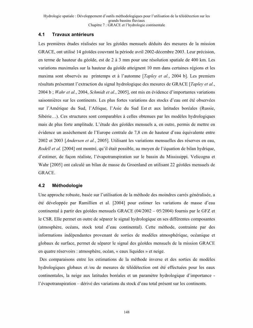
Hydrologie spatiale : Développement d’outils méthodologiques pour l’utilisation de la télédétection sur les
grands bassins fluviaux
Chapitre 7 : GRACE et l’hydrologie continentale
148
4.1 Travaux antérieurs
Les premières études réalisées sur les géoïdes mensuels déduits des mesures de la mission
GRACE, ont utilisé 14 géoïdes couvrant la période avril 2002-décembre 2003. Leur précision,
en terme de hauteur du géoïde, est de 2 à 3 mm pour une résolution spatiale de 400 km. Les
variations maximales sur la hauteur du géoïde atteignent 10 mm dans certaines régions et les
maxima sont observés au printemps et à l’automne [Tapley et al., 2004 b]. Les premiers
résultats présentant l’extraction du signal hydrologique des mesures de GRACE [Tapley et al.,
2004 b ; Wahr et al., 2004, Schmidt et al., 2005], ont mis en évidence d’importantes variations
saisonnières sur les continents. Les plus fortes variations des stocks d’eau ont été observées
sur l’Amérique du Sud, l’Afrique, l’Asie du Sud Est et aux latitudes boréales (Russie,
Sibérie…). Ces structures sont comparables à celles obtenues par les modèles hydrologiques
mais de plus forte amplitude. L’étude des géoïdes mensuels a, en outre, permis de mettre en
évidence un assèchement de l’Europe centrale de 7,8 cm de hauteur d’eau équivalente entre
2002 et 2003 [Andersen et al., 2005]. Utilisant les variations mensuelles des réserves en eau,
Rodell et al. [2004] ont montré, qu’il était possible, au moyen de l’équation de bilan hydrique,
d’estimer, de façon réaliste, l’évapotranspiration sur le bassin du Mississippi. Velicogna et
Wahr [2005] ont calculé un bilan de masse du Groenland en utilisant 22 géoïdes mensuels de
GRACE.
4.2 Méthodologie
Une approche robuste, basée sur l’utilisation de la méthode des moindres carrés généralisée, a
été développée par Ramillien et al. [2004] pour estimer les variations de masse d’eau
continental à partir des géoïdes mensuels GRACE (04/2002 – 05/2004) fournis par le GFZ et
le CSR. Elle permet en outre de séparer le signal hydrologique en ses différentes composantes
(atmosphère, océans, stock total d’eau continental). Cette méthode, contrainte par des
informations indépendantes provenant de sorties de modèles atmosphérique, océanique et
globaux de surface, permet de séparer le signal des géoïdes mensuels de la mission GRACE
en quatre réservoirs : atmosphère, océan, « eaux liquides » et neige.
Des comparaisons entre les estimations de la méthode inverse et des sorties de modèles
hydrologiques globaux et /ou de mesures de télédétection ont été effectuées pour les eaux
continentales, la neige aux latitudes boréales et un paramètre hydrologique d’importance -
l’évapotranspiration – dérivé des variations du stock d’eau total présent sur les continents.

Hydrologie spatiale : Développement d’outils méthodologiques pour l’utilisation de la télédétection sur les
grands bassins fluviaux
Chapitre 7 : GRACE et l’hydrologie continentale
149
5. Résultats
5.1 Validation de la méthode inverse
Résumé : La méthode inverse mise au point par Ramillien et al. [2004], convergeant, après
plusieurs itérations, au moyen de la technique des moindres carrés généralisées, permet
d’extraire, à l’échelle globale, les variations du stock d’eau sur les continents sous forme de
carte mensuelle de hauteur équivalente d’eau, à une résolution spatiale de ~660 kilomètres,
par combinaison de données spatiales et d’informations (a priori) issues de modèles
hydrologiques globaux. Différents tests ont permis de mettre en évidence la robustesse de la
méthode et ses capacités à séparer les estimations de masse d’eaux continentales en eaux
liquides (eaux de surface, humidité des sols et nappes phréatiques) et neige. Des comparaisons
avec les sorties du modèle hydrologique global Water Gap Hydrology Model (WGHM) [Döll
et al., 2003] montrent un bon accord à l’échelle de huit grands bassins tropicaux.

Time variations of land water storage from an inversion
of 2 years of GRACE geoids
G. Ramilliena,*, F. Frapparta, A. Cazenavea, A. Guntnerb
aLEGOS, 14 Avenue Edouard Belin, 31401 Toulouse Cedex 09, FrancebGeoForschungsZentrum (GFZ), Telegrafenberg, Potsdam, Germany
Received 1 December 2004; received in revised form 25 March 2005; accepted 5 April 2005
Available online 1 June 2005
Editor: V. Courtillot
Abstract
By delivering monthly maps of the gravity field, the GRACE project allows the determination of tiny time variations of the
Earth’s gravity and particularly the effects of fluid mass redistributions at the surface of the Earth. However, GRACE data
represent vertically integrated gravity measurements, thus are the sum of all mass redistributions inside the Earth’s system
(atmosphere, oceans and continental water storage, plus solid Earth). In this paper, we apply a generalized least-squares
inverse approach, previously developed by [1] [G. Ramillien, A. Cazenave, O. Brunau, Global time-variations of hydrological
signals from GRACE satellite gravimetry, Geophys. J. Int. 158 (2004) 813–826.], to estimate, from the monthly GRACE
geoids, continental water storage variations (and their associated uncertainties) over a 2-year time span (April 2002 to May
2004). Tests demonstrating the robustness of the method are presented, including the separation between liquid water
reservoirs (surface waters+soil moisture+groundwaters) and snow pack contributions. Individual monthly solutions of
total land water storage from GRACE, with a spatial resolution of ~660 km, are presented for the 2-year time span. We
also derive the seasonal cycle map. We further estimate water volume changes over eight large river basins in the tropics and
compare with model predictions. Finally, we attempt to estimate an average value of the evapotranspiration over each river
basin, using the water balance equation which links temporal change in water volume to precipitation, evapotranspiration and
runoff. Amplitudes of the GRACE-derived evapotranspiration are regionally consistent to the predictions of global hydro-
logical models.
D 2005 Elsevier B.V. All rights reserved.
Keywords: GRACE satellite gravimetry; global hydrology; least-squares inversion
1. Introduction
In March 2002, a new generation of gravity mis-
sions was launched: the Gravity Recovery and Cli-
mate Experiment (GRACE) space mission [2,3]. The
0012-821X/$ - see front matter D 2005 Elsevier B.V. All rights reserved.
doi:10.1016/j.epsl.2005.04.005
* Corresponding author. Tel.: +33 5 61 33 29 34.
E-mail address: [email protected] (G. Ramillien).
Earth and Planetary Science Letters 235 (2005) 283–301
www.elsevier.com/locate/epsl

objective of GRACE is to measure spatio-temporal
variations of the gravity field with an unprecedented
resolution and precision, over time scales ranging
from a few months to several years. As gravity is an
integral of mass, these spatio-temporal gravity varia-
tions represent horizontal mass redistributions only to
the extent that they are assumed to be caused by
surface loads. On time scales from months to dec-
ades, mass redistribution mainly occurs inside the
surface fluid envelopes (oceans, atmosphere, ice
caps, continental reservoirs) and is related to climate
variability. The main application of GRACE is quan-
tifying the terrestrial hydrological cycle through mea-
surements of vertically-integrated water mass changes
inside aquifers, soil, surface reservoirs and snow
pack, with a precision of a few millimeters in terms
of water height and a spatial resolution of ~400 km
[4,5].
Until the launch of GRACE, no direct measure-
ments of time-varying storage of snow, soil and
underground waters were available globally. There-
fore, the global distribution and spatio-temporal
changes of land water mass were essentially estimated
from modelling. The main motivation for developing
global land surface models (LSMs) over the recent
decades was to provide realistic temperature and
humidity boundary conditions to atmospheric models
developed for climate modelling. In effect, many land
surface parameters exert a strong influence on water
and energy surface fluxes and as a consequence on the
atmosphere. Among these parameters, soil moisture
and snow mass are important since they affect low-
atmosphere state on both short and long (seasonal and
inter-annual) time scales. Besides, land water storage
and snow mass are themselves affected by atmo-
spheric conditions and climate variability. In the
recent years, a number of state-of-the-art LSMs have
provided global gridded time series of soil water,
underground water and snow mass, typically on a
monthly basis and a geographical resolution of
~1818 (among others, [6–11]). These global hydro-
logical data sets are currently derived from model runs
either in a coupled mode or in a stand alone mode
forced by observations, in particular precipitation.
Due to the lack of global information on soil water
and snow depth, model validation is in general per-
formed by comparing predicted runoff with in situ
measurements in a number of river basins. Besides,
international projects for inter-comparing the global
hydrological models have been initiated in the recent
years (e.g., PILPS [12]; GSWP1 [13]). However,
these approaches remain limited and do not provide
a global evaluation of the models accuracy. Thus,
direct comparison of models outputs with independent
observations, in particular the GRACE-based hydro-
logical products, could be very instructive. However
at present, such comparisons first serve to evaluate the
precision of the GRACE products. Besides, they will
provide the basis for future space data assimilation
into the global hydrological models.
This paper presents results of monthly land water
change over 2 years (from April 2002 to May 2004)
from the GRACE geoids recently released by the
GRACE project [2]. The method developed in this
study differs from previously published GRACE
results [3,14,15] in that it tries to separate mass signals
from four different surface reservoirs (soil plus under-
ground plus surface water reservoirs, snow pack,
atmosphere and ocean) through an inverse modelling
based on generalized least-squares adjustment [16].
The inverse approach which combines the GRACE
observations with stochastic properties of the hydro-
logical (or oceanic) signal significantly reduces the
recovered land (or ocean) water signal compared to
the direct conversion of geoid anomalies into water
mass, because of noise reduction and elimination of
unrelated signal (e.g., atmospheric noise).
2. The GRACE geoids
The data set recently provided to GRACE users by
the GRACE project consists of monthly sets of sphe-
rical harmonic geoid coefficients (and associated
uncertainties), up to degree and order 100, since
April 2002. These coefficients derived from raw
tracking measurements (GRACE consists of a pair
of satellites whose mutual distance, absolute positions
and velocities are continuously monitored) are cur-
rently computed by two groups: the Center for Space
Research (CSR) in the USA and the GeoForschungs-
Zentrum (GFZ) in Germany. The geoid coefficients
are corrected for atmospheric loading and oceanic
tides. An a priori model for the oceanic variability
was also removed during the GRACE data processing.
Therefore, temporal changes of the geoid coefficients
G. Ramillien et al. / Earth and Planetary Science Letters 235 (2005) 283–301284

mainly represent change in continental water storage,
non-tidal oceanic effects and residual atmospheric
noise. In this study, we use the CSR geoid data,
spanning from April 2002 to May 2004. Fig. 1 dis-
plays the temporal coverage of this data set. The
length of the horizontal bars corresponds to the num-
bers of days used to construct each monthly geoid
from the raw measurements. Because of too few
usable raw measurements, a single monthly geoid is
provided for April–May 2002. For 2003, the May
geoid is a combination of April plus May data.
Although the spherical harmonic coefficients of each
monthly geoid are given up to degree and order 100,
in this study we follow earlier studies [3,14,15] and
only consider harmonic coefficients up to degree 30
(half horizontal wavelength of 660 km). In effect as
shown by Tapley et al. [3] and Schmidt et al. [15], at
higher degrees – shorter wavelengths – the signal to
noise ratio is too low due to residual errors in the data
processing that are not yet totally controlled. As in
previous studies, we also fix the degree 2, order 0
harmonic (half wavelength of 10000 km) to zero
because of the current large uncertainty associated
with this coefficient.
3. Methodology
3.1. The direct problem
3.1.1. Modelling geoid variations from the different
global model forecasts
The static component of the gravity field G0 cor-
responds to nearly 99% of the total field, mainly due
to solid Earth contributions. This term can be easily
evaluated and removed by computing the temporal
mean of a long enough series of GRACE monthly
geoids, or considering a single geoid computed with a
long period of time of satellite observations. In this
study, the monthly time-variable geoid yG(t) is merely
computed as the difference between the monthly
geoid G(t) measured by GRACE at time t, and the
static mean field component:
yG tð Þ ¼ G tð Þ G0 ð1Þ
Using the 20 monthly geoids, we computed a 2-
year mean geoid which was further removed to each
individual monthly geoid. This allows removal of the
static geoid contributions related to the Earth’s inter-
nal structure as well as to any dlong-termT surface
AVAILABLE MONTHLY GRACE GEOIDS FROM CSR
2002.25 2002.50 2002.75 2003.00 2003.25 2003.50 2003.75 2004.00 2004.25 2004.50 2004.75
TIME (years)
JAN 04
SEP 02
FEB 03
NOV 02
FEB 04
APR 04
OCT 02
APR/MAY 03
SEP 03
MAY 04
AUG 02
APR 03
NOV 03
JUL 03
AUG 03
DEC 03
APR/MAY 02
MAR 03
OCT 03
MAR 04
Fig. 1. Temporal coverage of the GRACE geoids provided by CSR (University of Texas) covering the period from 04/2002 to 05/2004 (each bar
corresponds to ~1-month time span).
G. Ramillien et al. / Earth and Planetary Science Letters 235 (2005) 283–301 285

fluid signal (e.g., deep, slowly-varying aquifers) that
cannot be extracted with only 2 years of data. Thus,
the corresponding geoid differences (also called
monthly GRACE geoids in the following) only
reflect short-term geoid change associated with sur-
face mass redistributions.
Let yCnm(t) and ySnm(t) be the bnormalizedQ
Stokes coefficients expressed in terms of millimeters
of geoid height, where n and m are the degree and
order respectively. The time-variable geoid is thus
expressed as:
yG tð Þ ¼X
N
n¼1
X
n
m¼0
yCnm tð Þcos mkð Þð
þ ySnm tð Þsin mkð ÞÞPnm coshð Þ ð2Þ
where N is the maximum degree of the decomposi-
tion, h is the co-latitude, k is the longitude and Pnm is
the associated Legendre polynomial which is dimen-
sionless. Assuming that the global fluid contributions
are not correlated in time and space, we consider that
yG(t) is the sum of k =1, 2, . . ., K fluid contributions:
yG tð Þ ¼X
K
k¼1
yGk tð Þ ¼ XyG ð3Þ
whereX is the bseparatingQmatrix formed by a column
of identity-blocks that ensures the non-correlation
between the geoid coefficients of the different fluid
contributions. Let yq(t) be a surface density associated
with surface water mass, expressed in terms of equiva-
lent-water thickness at time t, whose harmonic coeffi-
cients, yAnm(t) and yBnm(t), can be used to evaluate the
corresponding geoid anomaly coefficients by filtering:
yCnm tð ÞySnm tð Þ
¼ WnyAnm tð ÞyBnm tð Þ
ð4Þ
where Wn is an isotropic spatial filter that weights the
surface density coefficients, and whose analytical
expression is [17]:
Wn ¼2pGReqW2nþ 1ð Þc hð Þ
1þ znð Þ ð5Þ
where zn represents the Love numbers that enable to
take into account the elastic compensation of the Earth
to surface load. c(h) is the normal gravity on the
reference ellipsoid at the co-latitude h. G
(~6.67 d 1011 m3 kg1 s2) is the gravitational con-
stant and Re (~6378 km) is mean Earth’s radius. qW
(~1000 kg m3) is the water density. The latter equa-
tion is used to compute the geoid harmonic coefficients
from monthly surface density grids yq(h, k, t) and
provided either by global oceanic/hydrological models
or atmospheric surface pressure observations. The
corresponding Stokes coefficients are defined by [18]:
yCnm tð ÞySnm tð Þ
¼1þ znð ÞR2
e
2nþ 1ð ÞM
Z Z
S
yq h; k; tð Þ
cos
sin
mkð ÞPnm coshð ÞyS ð6Þ
since redistributions of fluid mass yqyS on the surface
of the Earth produce variations of the Stokes coeffi-
cients, taking the elastic compensation of the Earth’s
crust into account. M is the total mass of the Earth
(~5.97602 d 1024 kg).
Note that in case of atmospheric surface pressure or
ocean bottom pressure yp(h, k, t) data, commonly
expressed in Pa or N/m2, the corresponding surface
density variation yq(h, k, t) is:
yq h; k; tð Þ ¼yp h; k; tð Þ
qWc hð Þ: ð7Þ
In practice, once yq is computed for each time step
from model outputs using Eqs. (6) and (7), each sur-
face density grid is decomposed into spherical harmo-
nics yAnm(t) and yBnm(t), and then converted into
corresponding geoid coefficients yCnm(t) and
ySnm(t) by applying the direct filtering procedure
(Eq. (4)).
These time-series of bmodel/dataQ coefficients
represent the a priori information that will be used
as input in the inversion (described in the next sec-
tion). For each fluid contribution k and for each time
step t, it consists of: an initial solution used as bfirst
guessQ; an a priori model uncertainty matrix; and a
model covariance matrix that described the statistical
relationship between the geoid coefficients of a given
fluid reservoir k at time t.
3.1.2. Estimation of the a priori model uncertainties
A priori uncertainties on model harmonic coeffi-
cients are derived from statistical comparisons
between the geoid coefficients derived from the dif-
ferent oceanic/hydrological models associated with
each reservoir k. They are simply computed as the
G. Ramillien et al. / Earth and Planetary Science Letters 235 (2005) 283–301286

time variances of these coefficients for each month of
the year and over the longest time span available.
These variances are used as the diagonal elements of
the model covariance matrix CM.
3.1.3. Estimation of the a priori model covariances
To estimate the model covariance matrix Ck(t)
from geoid coefficients, we consider Dk(Dt), the
matrix formed by the list of all geoid coefficients
previously computed for the fluid reservoir k and
over a time period Dt. By construction, the matrix
Dk(Dt) is such that each row corresponds to a parti-
cular month and each column to a given coefficient
yCnm(t) or ySnm(t). Then, the model covariance matrix
Ck(t) is simply estimated by computing the product:
Ck tð Þ ¼ Dk Dtð Þ DkPP
½ TDk Dtð Þ Dk
PP
½ ð8Þ
where DkPP
is the time-mean value of the model coeffi-
cients computed during Dt months. Several previous
tests made by inverting synthetic geoid data have
suggested that an optimal value for Dt would be the
2–3 months centred around the considered month t
(see [1]). Greater values of this time span give rise to
numerical smoothing, and thus provide a less precise
geoid solution. To estimate the spatial correlations
between couples of geoid coefficients of degrees
and orders u, v, n, m, respectively, the elements of
Ck(t) are multiplied by the weighting function c
defined by:
w u; v; n;mð Þ ¼ 2jn uj þ 1ð Þ12jm vj þ 1ð Þ1
ð9Þ
3.2. The inverse approach for separating the fluid
mass contributions
The numerical strategy for separating the contribu-
tions of the different reservoirs was previously pre-
sented in [1]. It is based on the matrix formalism of
the generalized least-squares criteria developed by
Tarantola [16]. It consists of estimating separately
the spherical harmonic coefficients, in terms of
equivalent-water heights, of different fluid reservoirs
(atmosphere, oceans, soil waters and snow pack) from
the monthly GRACE geoids. For each water mass
reservoir, the solution is a linear combination of the
coefficients measured by GRACE, of the a priori
information from climate models and optimal coeffi-
cients fitting:
Ck tð Þ ¼ C0k tð Þ þ CkX CD þ CM þ XCkX
T 1
COBS tð Þ XC0k tð Þ
ð10Þ
where Ck(t) is the vector formed by the list of all
spherical harmonic coefficients of the geoid to be
solved for the k-th contribution, COBS(t) is the vector
formed with the geoid coefficients from GRACE,
Ck0(t) corresponds to the initial solution coefficients
vector (i.e. bfirst guessQ). CD and CM are the a priori
covariance matrices of the GRACE geoid coefficients,
and of the models, respectively. The latter matrix and
the vector Ck0(t) are estimated from the geoid coeffi-
cients derived from global model outputs for each
month (see previous section).
In practice, the matrix to be inverted (terms in
parenthesis in Eq. (10)) is symmetric by construction,
and often positive definite. We used a strategy of fast
Cholesky factorisation to solve this system, instead of
a LU decomposition. In extreme conditions of ill-
conditioning of the system, we also chose to apply a
complete Singular Value Decomposition (SVD) but
this is a more time-consuming option.
After solving the linear system (Eq. (10)), the a
posteriori covariance matrix CkPOS is computed using:
CPOSk ¼ Ck CkX
T XCkXT þ CD þ CM
1XCk :
ð11Þ
The a posteriori uncertainties associated to the
fitted geoid coefficients of the reservoir k are given
by the root-mean square values of the diagonal ele-
ments of CkPOS:
rPOSk tð Þ ¼ffiffiffiffiffiffiffiffiffiffiffiffiffiffiffiffiffiffiffiffiffiffi
CPOSk diagð Þ
q
ð12Þ
where bdiagQ stands for individual-diagonal elements
of the a posteriori matrix.
The estimated surface density coefficients
yAPOSnm (t) and yBPOS
nm (t), expressed in terms of
equivalent-water height, are then estimated by filter-
ing the fitted geoid coefficients yCPOSnm (t) and
G. Ramillien et al. / Earth and Planetary Science Letters 235 (2005) 283–301 287

ySPOSnm (t) listed in the solution Ck(t) of each reservoir k
using:
yAPOSnm tð Þ
yBPOSnm tð Þ
¼ VnW1n
yCPOSnm tð Þ
ySPOSnm tð Þ
ð13aÞ
with:
Vn¼
1 if nbnmin
1
2cos p
n nmin
nmax nmin
if nminVnVnmax
0 if nNnmax
8
>
<
>
:
ð13bÞ
whereWn1 is the inverse predicting filter of Eq. (4). It
is tapered by a stabilizing function Vn that apodises the
amplitudes ofWn1 for degrees between nmin and nmax,
in order to avoid the development of spurious short-
wavelength undulations. Obviously, the main disad-
vantage of using such a smoothed operator is to
remove short-wavelength details in the solution, but
this is necessary to avoid numerical instabilities in the
matrix inversion of the system (Eq. (10)), and to cancel
the effects of noise for high-degrees (typically
nmin=25 and nmax=30).
An iterative process was implemented. Tests have
shown that convergence was obtained after ~5 itera-
tions. Thus solutions presented in Section 4 corre-
spond to the 5th iteration.
3.3. Model outputs used for the inversion
To construct the bfirst guessQ as well as the Ck
covariance matrices, we considered the following
models:
3.3.1. Land hydrology
– LaD model [9]
– WGHM model [11]
The Land Dynamics (LaD) model developed by
Milly and Shmakin [9] estimates the time-varying
storage of snow, root-zone soil water and ground
water by solving water and energy balance equations
which relate temporal change in storage to rainfall,
snowfall, evapotranspiration, sublimation, snow melt,
soil water drainage and ground water discharge to
streams. The model provides 1818 monthly global
grids of snow, root-zone soil water, underground
waters (from the shallow and dynamic unconfined
saturated zone) for 1981–2003.
The Water GAP Global Hydrology Model
(WGHM) [11] was specifically designed to estimate
river discharge for water resources assessments. It
computes 0.580.58 gridded time series of monthly
runoff and river discharge and is tuned against time
series of annual river discharges measured at 724
globally distributed stations. Other products of the
model are monthly gridded time series of water storage
in the snow cover, soil water within the root zone,
ground water and surface water stored in rivers, lakes
and wetlands. The data are available for 2002 to 2004.
3.3.2. Ocean bottom pressure
We used ocean bottom pressure data derived from
two Ocean Global Circulation Models (OGCMs):
– POCM-4C (Parallel Ocean Circulation Model)
[19,20]
– ECCO [21]
While initial resolutions and time spans of ocean
bottom pressure grids provided by these models are
different, we interpolated the data onto 1818 grids
and constructed a climatology (standard year).
3.3.3. Atmosphere
Atmospheric loading effects were removed during
the GRACE data processing. However, in order to
account for any residual atmospheric signal in the
GRACE geoid, we considered a dresidual
atmosphereT reservoir for the inversion. Thus, to
construct the corresponding covariance matrix, we
used gridded differences between two atmospheric
surface pressure data sets: NCEP [22] and ECMWF.
These gridded differences were further developed
into spherical harmonics, and corresponding coeffi-
cients, in units of equivalent water height were further
expressed in terms of geoid height (see [1]).
3.4. Deriving time-series of water mass variations
from monthly geoids: test results
As indicated above, we separated the contributions
of four different equivalent-water mass reservoirs: soil
plus underground plus surface waters reservoir (called
dliquid reservoirT in the following), snow pack, resi-
G. Ramillien et al. / Earth and Planetary Science Letters 235 (2005) 283–301288

Fig. 2. (a) Land water solution for April 2003 for the nominal case after 5 iterations; (b) WGHM land water storage for April 2003; (c) log of
errors for the input geoid (upper curve), model (middle curve) and nominal solution (lower curve) for April 2003, as a function of harmonic
degree; (d) difference in land water storage between GRACE and WGHM; (e) residual geoid for April 2003; (f) land water solution after 10
iterations with first guess set to zero, (g) convergence curves for the nominal case and first guess set to zero.
G. Ramillien et al. / Earth and Planetary Science Letters 235 (2005) 283–301 289

dual atmosphere and ocean, from each of the 20
months (from April/May 2002 to May 2004). For
constructing the dfirst guessT as well as the model
covariance and model error matrices, the following
models have been considered for defining the
dnominalT case: ECCO for the ocean bottom pressure,
the difference ECMWF minus NCEP for the residual
atmospheric signal, and WGHM for land waters
(liquid water reservoirs and snow pack). The nominal
land water solution (sum of liquid waters plus snow
Fig. 2 (continued ).
G. Ramillien et al. / Earth and Planetary Science Letters 235 (2005) 283–301290
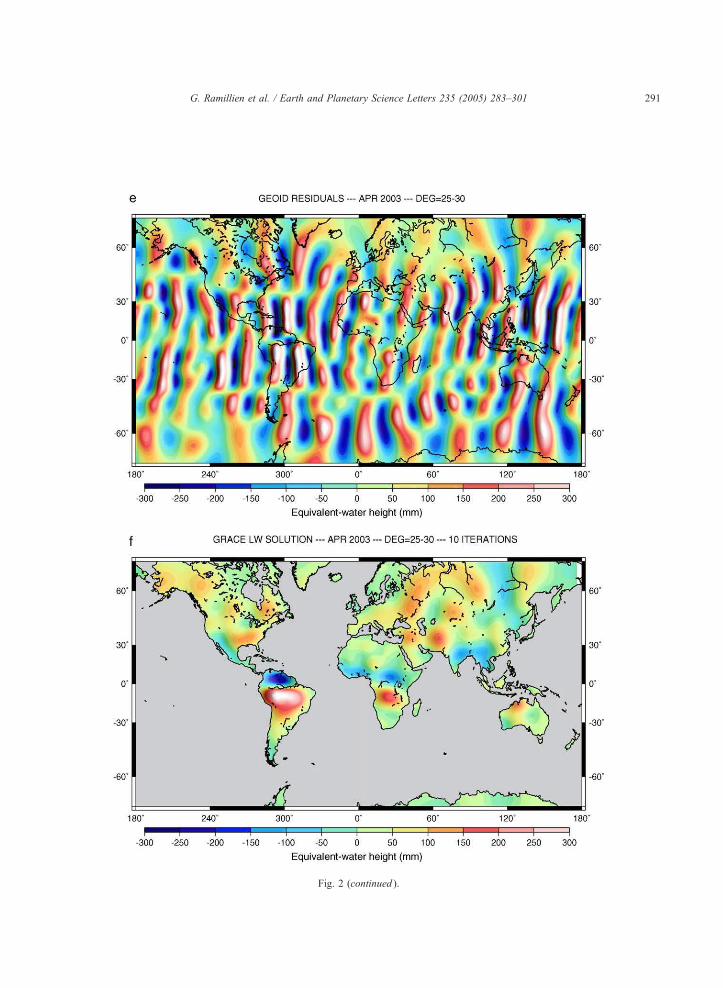
Fig. 2 (continued ).
G. Ramillien et al. / Earth and Planetary Science Letters 235 (2005) 283–301 291

mass), up to degree 30, for April 2003, based on the
inversion of the GRACE geoid, is presented in Fig.
2a. It corresponds to the solution obtained after 5
iterations, when convergence was reached. For com-
parison, the WHGM prediction (sum of all water
components) – up to degree 30 – is shown in Fig.
2b. The error spectra as a function of harmonic degree
for the input geoid, the solution and the model are
plotted in Fig. 2c. We note that the a posteriori errors
of the solution are smaller (almost by a factor 10) than
the model errors and GRACE input geoid errors. The
a posteriori errors decrease with increasing degree up
to degree 15, and then increase progressively, follow-
ing the spectrum behaviour of a priori observed uncer-
tainties. Fig. 2d and 2e show maps of the differences
between the GRACE solution and the model, and the
residual geoid based on the difference between the
GRACE geoid and the geoid solution constructed
using the solutions of the inversion for the four reser-
voirs (total soil water, snow, residual atmosphere and
ocean). Fig. 2d shows positive signal in a number of
regions, in particular over the Amazon basin, an indi-
cation that the GRACE solution contains more power
than predicted by the model. The residual geoid map
(Fig. 2e) is dominated by north–south strips of ampli-
tude in the range F300 mm (equivalent water height).
These strips are also seen in the input GRACE geoid
and may result from a combination of noise and Gibbs
oscillations associated with the spherical harmonic
cut-off at degree 30. The fact that the residual geoid
presents the same strips as in the input geoid is
comforting. It means that the GRACE geoid noise
was not incorporated into the solution and that the
inversion process was efficient.
We further performed a series of tests – for April
2003 – to evaluate the robustness of the solution. The
discussion here is limited to the land water storage
solution. The tests concern different first guesses (for
land water storage) as input (WGHM and LaD, and an
extreme case with the first guess set to zero), an error-
free model assumption (a priori covariance matrix CM
set to zero), a model error larger than the nominal case
(covariance matrix CM elements multiplied by 100),
data errors set to zero, etc. The land water solution for
the error-free model case is almost identical to the
nominal solution while the large model error case
provides a solution very close to the first guess
(WGHM solution). The case with no error in the
data gives rise to a very noisy (high-amplitude
north–south strips) in the land water solution. Finally
DIFF OBSERVED GEOID MINUS LW SOLUTION --- APR 2003
0.0
0.5
1.0
1.5
2.0
2.5
3.0
3.5
4.0(R
ms
ampl
itude
x 1
03 ) (m
m)
0 1 2 3 4 5 6 7 8 9 10 11 12
Number of iterations
First Guess = WGHM
First Guess = LAD
First Guess = ZERO
g
Fig. 2 (continued ).
G. Ramillien et al. / Earth and Planetary Science Letters 235 (2005) 283–301292

Fig. 3. Example of an efficient separation of hydrological components for April 2003 (5-iteration solutions, degree maximum 25–30): (a) total
(liquid) water solution (surface waters+soil moisture+groundwater) and (b) snow depth solution.
G. Ramillien et al. / Earth and Planetary Science Letters 235 (2005) 283–301 293

the case with first guess set to zero is interesting. After
one iteration, the solution shows the familiar pattern
of the nominal solution and model but the amplitudes
of the water mass anomalies are on the average a factor
of 2 smaller. After 10 iterations, the solution displays
anomalies amplitudes in good agreement with the
nominal case (Fig. 2f). We note, however, that the
solution is slightly smoother (less short wavelength
signal) than in the nominal case. This point needs
further investigation. Finally, Fig. 2g presents the
root mean square residuals between the GRACE
geoid and the reconstructed geoid, as a function of
iteration rank, for the nominal case, a case with LaD as
first guess, and the case with the first guess set to zero.
As expected, the convergence is slower when the first
guess is set to zero. However, the three cases provide
similar convergence behaviour after ~5 iterations.
We next present the individual solutions for liquid
water (soil plus underground plus surface reservoirs)
(Fig. 3a) and solid water (snow pack) (Fig. 3b). It
appears that the inversion process does rather well in
separating the liquid and solid water components,
even though we note some contaminating signal in
the snow map over the Amazon basin, which evi-
dently should not be there. This means that some
improvement in the inversion method is still needed.
3.5. Comparison with the results provided by the
Wahr et al. [4] method
The approach we propose differs from the Wahr et
al. filtering by the fact it is an inversion, which
combines different a priori information (i.e. model
forecasts, errors and GRACE observations) to
improve iteratively a bfirst guessQ. The solution is
linearly corrected by GRACE data through covariance
matrices in space and time.
Early work of Jekeli [23] inspired Wahr and Mole-
naar [4] to propose a method based on the Gaussian
averaging of the Stokes coefficients observed by
GRACE to remove the effects of the noise at high
harmonic degrees. Given the half-height length L, the
Jekeli’s smoothing operator J versus degree n is
defined by an iterative relation:
J0 ¼1
2p; J1 ¼
1
2p
1þ e2b
1 e2b
;
Jnþ1 ¼ 2nþ 1
bJn þ Jn1 ð14Þ
where the parameter b is:
b ¼ln2
1 cos L=Reð Þ: ð15Þ
Fig. 4. Continental water storage variations over the Amazon basin for April 2003 derived using two approaches: (a) linear filtering from Wahr
and Molenaar [4] (L=650 km); (b) land water solution after 5 iterations using the proposed inverse method.
G. Ramillien et al. / Earth and Planetary Science Letters 235 (2005) 283–301294

This filtering was also used by Tapley et al. [3]
and Schmidt et al. [15] to compute the maps of the
continental water storage changes from monthly
GRACE geoids. These studies used a value of 750
km (degree 27) for L as a good compromise between
spatial resolution and effect of noise. Wahr and
Molenaar [4] predicting filter Wn to derive coeffi-
cients of equivalent-water from the geoid anomaly
ones is:
Wn ¼3qW 1þ znð Þ
qe 2nþ 1ð Þð16Þ
where qe is the mean Earth’s density (~5517 kg/m3).
This latter operator is numerically equivalent to the
one defined earlier in Eq. (5).
Fig. 4 presents results in the region of Amazon
basin comparing this approach and ours over the
Amazon basin for April 2003. For the Wahr et al.
method, we used L=650 km, which corresponds to
our cut-off harmonic degree (degree 30).
Amplitudes of the two maps are comparable, and
range between F300 mm of equivalent-water height.
However, differences are regionally important (the
rms difference is 86.83 mm over the Amazon
basin), and mainly due to a shift of the principal
maxima of the water storage changes from one solu-
tion to the other. The inversion-derived solution
shows more short-wavelength details, with the posi-
tive anomaly in closer agreement with the model
predictions (see Fig. 2), more centred over the basin
and less leakage on the oceanic areas.
4. Land water solutions from GRACE: results
4.1. Time series of monthly solutions
Six of the 20 monthly solutions for the total land
water storage (sum of liquid water storage plus snow)
are presented in Fig. 5a–f. These six maps correspond
to the months of July 03, September 03, November
03, January 04, March 04 and May 04. The 20 solu-
tions are based on the nominal case discussed in
Section 3. Because the year 2003 is almost complete
(only January and June are lacking), compared to the
other 2 years, we restrict our discussion to that parti-
cular period. The largest signals are observed in large
tropical river basins (Amazon and Orinoco basins in
South America, Congo and Niger basins in Africa,
Ganges and Bramhaputra basins in India) as well as
in several river basins of the northern hemisphere
(Mississippi basin in North America, Ob and Lena
rivers basins in northeast Asia, Volga basin in eastern
Europe). In high latitude regions, month to month
changes are also clearly visible (Alaska, eastern and
western Canada, northern Asia). In these high latitude
regions, the observed signal results from the combined
contributions of total soil water and snow. In general,
the solutions agree well with the models as far as the
geographical positions of the anomalies are concerned.
In terms of relative amplitude, the solutions differ
significantly from the models however, as do the mod-
els each other. We note however a better agreement
with WGHM than with LaD (not shown). We com-
puted maps of the differences between the GRACE
solutions (total soil water plus snow) and the WGHM
model (not shown, except for April 2003; see Fig. 2c).
Amplitude differences of individual months can reach
up toF100 mm in terms of water height. Comparisons
with the individual solutions and model predictions
indicate that there is no systematic underestimation
by the model. It clearly depends on the region.
4.2. Seasonal cycle
From the individual monthly solutions available,
we have constructed a seasonal cycle solution.
For that purpose, we assumed that the GRACE-
derived changes of water continental mass yq(h, k, t)
are the sum of a linear trend, a seasonal sinusoid
(which pulsation is x ¼ 2pT, with T ~1 year) and
water mass residuals yqRES(h, k, t):
yq h; k; tð Þ¼ a h; kð Þt þ b h; kð Þ½
þ n h; kð Þcos xtþ h;kð Þð Þ½ þyqRES h; k; tð Þ
ð17Þ
The parameters which we adjusted for each grid
point (h, k) are the linear trend (i.e. slope a(h, k) and
b(h, k)), and then the seasonal cycle (i.e. amplitude
n(h, k) and phase u(h, k)) after being corrected from
the temporal trend. For this purpose, we used a least-
squares fitting to solve the system:
yQ ¼ UdX ð18Þ
G. Ramillien et al. / Earth and Planetary Science Letters 235 (2005) 283–301 295

where the vector yQ is the list of the GRACE-derived
LW values, U and X are the configuration matrix and
the parameter vector, respectively. The latter two
terms are successively:
U ¼ t tj 1 b; and X ¼ a b½ ð19Þ
for adjusting the temporal trend, and:
U ¼ t cos xtj
sin xtj
b; and X¼ ncosu nsinu½
ð20Þ
for fitting the seasonal amplitude and phase at each
grid point. In both cases, according to the least-
Fig. 5. Monthly land waters (sum of liquid water reservoirs and snow pack) solutions (after 5 iterations) for 6 months of the 20 computed
solutions (nominal case).
G. Ramillien et al. / Earth and Planetary Science Letters 235 (2005) 283–301296

Fig. 6. Results of the least-squares adjustment of the seasonal amplitudes: (a) for land water storage from GRACE; and (b) for the WGHM
model.
G. Ramillien et al. / Earth and Planetary Science Letters 235 (2005) 283–301 297

squares criteria, the solution vector of the system
is:
X SOL ¼ UTU 1
UTyQ ð21Þ
The amplitude maps of the observed and model
seasonal cycles are presented in Fig. 6a and b.
Looking at Fig. 6a and b, we note that the GRACE
seasonal cycle presents in some regions higher ampli-
tude than WGHM, principally in the tropical river
basins. In South America, the maximum GRACE
signal is located at the southern edge of the Amazon
river while in the model, it coincides with the river.
Moreover, the GRACE seasonal amplitude map
clearly shows a large signal over the Orinoco basin,
not seen in WGHM.
We further looked at the interannual signal. We
first considered several couples of similar months of
years 2002, 2003 and 2004 and computed the differ-
ences. In these cases, the signal is evidently smaller
than at the seasonal time scale, but clear inter-annual
anomalies are visible over several basins of the north-
ern hemisphere (e.g., the Ob and Lena basins in
Siberia) as well as over tropical basins (Orinoco,
Amazon, Niger, Congo and Ganges).
5. Time-series of water volume change in large
river basins
At a given month t, the regional variation of water
volume yV(t) over a given river basin S is the sum of
the products of the GRACE-derived surface load yqj,
with j=1, 2, . . . (expressed in terms of equivalent-
water height) inside S, by the elementary surface
Re2ykyhsinhj:
yV tð Þ ¼ R2eykyh
X
jaS
yqj h; k; tð Þsin hj
ð22Þ
where yk and yh are the sampling grid steps along
longitude and latitude, respectively. In practice, the
points of S used in Eq. (22) are extracted over eight
drainage basins located in the tropics (Amazon, Ori-
noco, Tocantins, Parana, Congo, Niger, Ganges and
Mekong). The contour of each basin is based on
masks of 0.58 resolution from Oki and Su [24]. The
locations of the eight drainage basins are presented in
Fig. 7. Fig. 8 displays the temporal water volume
change – spatially averaged – over each basin for
the 2 years. The predicted volume change from the
WGHM model is also shown. We note in general
good amplitude agreement with the model predictions
for some basins: Amazon, Orinoco, Congo, Mekong.
180˚
180˚
240˚
240˚
300˚
300˚
0˚
0˚
60˚
60˚
120˚
120˚
180˚
180˚
-60˚ -60˚
-30˚ -30˚
0˚ 0˚
30˚ 30˚
60˚ 60˚
180˚
180˚
240˚
240˚
300˚
300˚
0˚
0˚
60˚
60˚
120˚
120˚
180˚
180˚
-60˚ -60˚
-30˚ -30˚
0˚ 0˚
30˚ 30˚
60˚ 60˚
2 6
4
5
7 8
1 3
Fig. 7. Location maps of the eight studied drainage basins. 1: Orinoco; 2: Amazon; 3: Tocantins; 4: Parana; 5: Niger; 6: Congo; 7: Ganges; 8:
Mekong.
G. Ramillien et al. / Earth and Planetary Science Letters 235 (2005) 283–301298

Fig. 8. Time series of total water volume (average over the basin area) based on GRACE (solid curve), on the WGHMmodel (dashed curve) and
estimate the mean evapotranspiration (dotted curve), for each of the eight studied basins.
G. Ramillien et al. / Earth and Planetary Science Letters 235 (2005) 283–301 299

For the Tocantins and Parana basins, the GRACE-
derived water volumes are larger than model predic-
tions. Poor agreement is noticed for the Ganges and
Niger basins. Additional model comparisons need to
be performed in the future.
We further attempted to provide an estimate of the
mean evapotranspiration for each basin. For that pur-
pose, we considered the water mass budget equation:
dV
dt¼ P E R ð23Þ
with V: land water storage, P: precipitation, E: evapo-
transpiration, R: runoff. We computed the derivative,
dV/dt, of the water volume change using the GRACE
solutions, subtracted the precipitation P averaged over
the basin (using data from the Global Precipitation
Climatology Centre [25,26]), and further subtracted
the mean runoff R over the basin using outputs of
the WGHM model. Finally we estimated the evapo-
transpiration E. For each basin, mean (i.e., averaged
over the basin area) evapotranspiration curve is super-
imposed to the observed and model volume curves in
Fig. 8. Evapotranspiration is a key-component of
hydrological budget at the local/regional scale. This
parameter is presently poorly described due to lack of
measurements and modelling complexity. Werth and
Avissar [27] summarize the contradictions of several
datasets of Amazonian evapotranspiration: Global Cli-
mate Models tend to produce an evapotranspiration
cycle that follows the precipitation cycle – mostly
during the rainy austral summer (December–February)
and less during drier austral winter (June–August) –
whereas models of evapotranspiration derived from
observations of net surface radiation and atmospheric
humidity provide a weak annual cycle that is out of
phase with that of precipitation. Note however that the
estimates of the mean evapotranspiration presented
here for the Amazon basin are in relatively good
agreement with the NCEP-derived evapotranspiration
reported in [27], both in phase and amplitude. From the
results presented in Fig. 8, we note that over equatorial
basins (i.e. Amazon, Congo), the annual cycle is not
well marked whereas a strong annual cycle is present
in the tropical basins (i.e., Parana, Orinoco, Tocantins,
Niger, Ganges and Mekong). Besides, the annual cycle
of evapotranspiration appears correlated with the pre-
cipitation cycle in the latter regions. Over the Amazon
basin, the annual mean evapotranspiration rate is of
600 km3/month or 3.3 mm/day. These values can be
compared with the modelled and observational esti-
mates of Costa and Foley [28] who have found respec-
tively 3.66 and 3.27 mm/day for the whole basin, 4.18
and 4.12 over the rain forest.
6. Conclusion
In this study, we present new solutions of time
variations in continental water storage from the avail-
able GRACE geoids, over the period April 2002 to
May 2004. These solutions, with a spatial resolution
of 660 km, are based on a generalized least-squares
inversion that combines different model and data
errors information. The iterative version of the inver-
sion scheme rapidly converges towards a unique land
water solution. Moreover, the algorithm efficiently
filters out the spurious undulations present in the
input GRACE geoids. However, resolution and preci-
sion of the computed land water maps still need to be
improved, hopefully when uncertainties on the
observed GRACE coefficients (especially beyond
degree 30) will be reduced. From monthly land
water time series, we also estimate the temporal var-
iation of the mean evapotranspiration over eight large
drainage basins located in the tropics. It is based on
the water balance equation and the use of observed
precipitation and predicted runoff data. Since evapo-
transpiration remains a poorly known hydrological
parameter (because neither well-measured nor mod-
elled), its estimate based on monthly land water maps
derived from GRACE represents an interesting con-
tribution to global hydrology.
The entire series of maps of the 20 monthly bLand
WatersQ solutions can be downloaded from our labora-
tory web site: http://www.obs-mip.fr/umr5566/.
Acknowledgements
We thank the GRACE project for having made
available the monthly GRACE geoids. We also
thank C. Milly, P. Doll and J. Alcamo for providing
us with global outputs of their hydrological models, as
well as A. Tarantola and an anonymous reviewer for
helpful comments. One of us (FF) benefited from a
CNES-ALCATEL SPACE PhD grant.
G. Ramillien et al. / Earth and Planetary Science Letters 235 (2005) 283–301300

References
[1] G. Ramillien, A. Cazenave, O. Brunau, Global time-variations
of hydrological signals from GRACE satellite gravimetry,
Geophys. J. Int. 158 (2004) 813–826.
[2] B.D. Tapley, S. Bettadpur, M. Watkins, C. Reigber, The grav-
ity recovery and climate experiment: mission overview and
early results, Geophys. Res. Lett. 31 (2004) L09607,
doi:10.1029/2004GL019920.
[3] B.D. Tapley, S. Bettadpur, J.C. Ries, P.F. Thompson, M.
Watkins, GRACE measurements of mass variability in the
Earth system, Science 305 (2004) 503–505.
[4] J. Wahr, M. Molenaar, Time variability of the Earth’s gravity
field: hydrological and oceanic effects and their possible
detection using GRACE, J. Geophys. Res. 103 (B12) (1998)
30205–30229.
[5] M. Rodell, J.S. Famiglietti, Detectability of variations in con-
tinental water storage from satellite observations of the time
dependent gravity field, Water Resour. Res. 35 (9) (1999)
2705–2723.
[6] N.I. Ducoudre, K. Laval, A. Perrier, SECHIBA, a new set of
parameterizations of the hydrologic exchanges at the land
atmosphere interface within the LMD Atmospheric General
Circulation Model, J. Clim. 6 (2) (1993) 248–273.
[7] H. Douville, E. Bazile, P. Caille, D. Giard, J. Noilhan, L.
Peirone, F. Taillefer, Global Soil Wetness Project: forecast
and assimilation experiments performed at Meteo-France, J.
Meteorol. Soc. Jpn. 77 (1999) 305–316.
[8] H. Douville, F. Chauvin, Relevance of soil moisture for sea-
sonal climate predictions; a preliminary study, Clim. Dyn.
(2000) 16719–16736.
[9] P.C.D. Milly, A.B. Shmakin, Global modeling of land water
and energy balances: 1. The Land Dynamics (LaD) model, J.
Hydrometeorol. 3 (2002) 283–299.
[10] T. Ngo-Duc, J. Polcher, K. Laval, A 53-year forcing data set
for land-surface models, J. Geophys. Res. 110 (2005) D06116,
doi:10.1029/2004JD005434.
[11] P. Doll, F. Kaspar, B. Lehner, A global hydrological model for
deriving water availability indicators: model tuning and vali-
dation, J. Hydrol. 270 (2003) 105–134.
[12] Y. Shao, A. Henderson-Sellers, Modeling soil moisture: a
project for intercomparison of land surface parameterization
schemes Phase 2(b), J. Geophys. Res. 101 (1996) 7227–7250.
[13] P.A. Dirmeyer, A. Dolman, N. Sato, The pilot phase of the
Global Soil Wetness Project, Bull. Am. Meteorol. Soc. 80
(1999) 851–878.
[14] J. Wahr, S. Swenson, V. Zlotnicki, I. Velicogna, Time-variable
gravity from GRACE: first results, Geophys. Res. Lett. 31
(2004) L11501, doi:10.1029/2004GL019779.
[15] R. Schmidt, F. Flechtner, Ch. Reigber, P. Schwintzer, A.
Guntner, P. Doll, G. Ramillien, A. Cazenave, S. Petrovic, H.
Jochman, J. Wunsch, GRACE observations of changes in
continental water storage, Glob. Planet. Change (in press)
18, doi: 10.1016/j.gloplacha.2004.11.018.
[16] A. Tarantola, Inverse Problem Theory, Elsevier, Amsterdam,
1987, 613 pp.
[17] G. Ramillien, Gravity/magnetic potential of uneven shell topo-
graphy, J. Geod. 76 (2002) 139–149, doi:10.1007/s00190-
002-0193-5.
[18] W.H. Heiskanen, H. Moritz, Physical Geodesy, W.H. Freeman
and Co, San Francisco, 1967.
[19] D. Stammer, R. Tokmakian, A. Semtner, C. Wunsch, How well
does a 1/48 global circulation model simulate large-scale ocea-
nic observations? J. Geophys. Res. 101 (1996) 25799–25811.
[20] R. Tokmakian, Comparisons of time series from two global
models with tide-gauge data, Geophys. Res. Lett. 23 (1996)
3759–3762.
[21] D. Stammer, C. Wunsch, R. Giering, C. Eckert, P. Heimbach,
J. Marotzke, A. Adcroft, C.N. Hill, J. Marshall, The global
ocean circulation during 1992–1997, estimated from ocean
observations and a general circulation model, J. Geophys.
Res. 107 (C9) (2002) 3118, doi:10.1029/2001JC000888.
[22] R.E. Kistler, et al., The NCEP–NCAR 50-year reanalysis:
monthly means CD-ROM and documentation, Bull. Am.
Meteorol. Soc. 82 (2001) 247–267.
[23] C. Jekeli, Alternative Methods to Smooth the Earth’s Gravity
Field, Rep. 327. Dep. of Geod. Sci. and Surv., Ohio State
Univ., Columbus, 1981.
[24] T. Oki, Y.C. Su, Design of Total Runoff Integrating Pathways
(TRIP)—a global river channel network, Earth Interact. 2 (1)
(1998) 1–37.
[25] B. Rudolf, H. Hauschild, W. Rueth, U. Schneider, Terrestrial
precipitation analysis: operational method and required density
of point measurements, in: M. Desbois, F. Desalmond (Eds.),
Global Precipitations and Climate Change, NATO ASI Series
I, vol. 26, Springer-Verlag, 1994, pp. 173–186.
[26] B. Rudolf, T. Fuchs, U. Schneider, A. Meyer-Christoffer,
Introduction of the Global Precipitation Climatology Centre
(GPCC), Deutscher Wetterdienst, Offenbach a.M., p. 16.
[27] D. Werth, R. Avissar, The regional evapotranspiration of the
Amazon, J. Hydrometeorol. 5 (2004) 100–109.
[28] M.H. Costa, J.A. Foley, Water balance of the Amazon Basin:
dependence on vegetation cover and canopy conductance,
J. Geophys. Res. 102 (D20) (1997) 23973–23989.
G. Ramillien et al. / Earth and Planetary Science Letters 235 (2005) 283–301 301

Hydrologie spatiale : Développement d’outils méthodologiques pour l’utilisation de la télédétection sur les
grands bassins fluviaux
Chapitre 7 : GRACE et l’hydrologie continentale
169
5.2 Estimation des masses d’eaux continentales
De nombreuses études ont montré qu’il était possible de détecter les fluctuations temporelles
du contenu en eau des principaux bassins fluviaux [Rodell et Famiglietti, 1998 ; Swenson et
Wahr, 2003 ; Tapley et al., 2004 b]. La méthode développée par Ramillien et al. [2004]
permet d’estimer les variations mensuelles du stock d’eau continental. Ce dernier peut lui-
même être décomposé en un terme « eaux liquides » regroupant les eaux de surface et
l’humidité du sol, et un terme neige. La Figure 7-3 illustre la variabilité inter-annuelle des
solutions « eaux liquides », présente des cartes pour les mois d’avril-mai 2002, mai 2003 et
mai 2004. L’analyse des solutions eaux liquides (cartes mensuelles de résolution ~660 km)
montrent que les variations sont essentiellement annuelles, avec des amplitudes pouvant
atteindre jusqu’à ± 300 mm en terme de hauteur d’eau équivalente dans les grands bassins
équatoriaux et tropicaux, comme l’Amazone, le Congo ou le Gange (signal de mousson).
La composante annuelle du signal hydrologique a été estimée, en faisant l’hypothèse que les
changements de masse des « eaux liquides » déduits des mesures de GRACE δq(θ, λ, t)
étaient la somme d’une tendance linéaire, d’une sinusoïde et d’un résidu. La carte d’amplitude
annuelle est présentée Figure 7-4.
Avril-Mai 2002 Avril 2003 Avril 2004
Figure 7-3: Solutions "eaux liquides" pour les mois d'avril-mai 2002, mai 2003 et mai 2004.
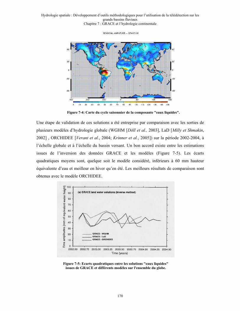
Hydrologie spatiale : Développement d’outils méthodologiques pour l’utilisation de la télédétection sur les
grands bassins fluviaux
Chapitre 7 : GRACE et l’hydrologie continentale
170
Une étape de validation de ces solutions a été entreprise par comparaison avec les sorties de
plusieurs modèles d’hydrologie globale (WGHM [Döll et al., 2003], LaD [Milly et Shmakin,
2002] , ORCHIDEE [Verant et al., 2004; Krinner et al., 2005]) sur la période 2002-2004, à
l’échelle globale et à l’échelle du bassin versant. Un bon accord existe entre les estimations
issues de l’inversion des données GRACE et les modèles (Figure 7-5). Les écarts
quadratiques moyens sont, quelque soit le modèle considéré, inférieurs à 60 mm hauteur
équivalente d’eau et meilleur en hiver qu’en été. Les meilleurs résultats de comparaison sont
obtenus avec le modèle ORCHIDEE.
Figure 7-4: Carte du cycle saisonnier de la composante "eaux liquides".
Figure 7-5: Ecarts quadratiques entre les solutions "eaux liquides"
issues de GRACE et différents modèles sur l'ensemble du globe.

Hydrologie spatiale : Développement d’outils méthodologiques pour l’utilisation de la télédétection sur les
grands bassins fluviaux
Chapitre 7 : GRACE et l’hydrologie continentale
171
Des séries temporelles de variations de masse (ou de volume) d’eau ont été calculées à partir
des cartes mensuelles, pour plusieurs grands bassins versants. Chaque mois, la variation de
volume d’eau δV(t), à l’intérieur d’un basin de surface S, est la somme des produits des
variations de masse déduites des mesures GRACE δqj, avec j=1, 2, … (exprimées en hauteur
équivalente d’eau) par la surface élémentaire Re2 δλ δθ sinθj :
)sin(),,()(2
j
Sjje tqRtV θλθδδλδθδ ∑= ∈ (Eq. 7-2)
où δλ et δθ sont les pas de grille en longitude et latitude et Re le rayon moyen de la Terre
(~6378 km). Les points de S utilisés dans Eq. 7-2 proviennent de masques de 0,5° de
résolution, fournis par Oki et Sud [1998].
A l’échelle régionale ces séries temporelles de variations de volume d’ « eaux liquides »
(Figure 7-6) sont en accord avec celles issues des modèles globaux, avec des erreurs
quadratiques de l’ordre de 30 à 40 mm.
L’accord entre les séries temporelles de GRACE et celles des modèles est fonction de la
localisation géographique du bassin et de sa taille. De plus fortes différences sont observées
Figure 7-6:Séries temporelles de variations de volume d'eau dans 16 grands bassins fluviaux. En
noir les estimations de GRACE, en pointillés de LaD et en gris de WGHM.

Hydrologie spatiale : Développement d’outils méthodologiques pour l’utilisation de la télédétection sur les
grands bassins fluviaux
Chapitre 7 : GRACE et l’hydrologie continentale
172
pendant l’hiver sur les bassins des hautes latitudes, couverts par la neige, comme la Volga,
l’Ob ou la Yenissey. De possibles contaminations des solutions « eaux liquides » par du
signal lié à la neige est plausible. Concernant la taille du bassin, la résolution des données
GRACE ne permet pas la détection des petites structures. La taille minimale critique des
bassins étudiés est de l’ordre de 250 000 km².
Une première comparaison entre les variations totales de volume d’eau observées par GRACE
et les variations d’eau de surface estimées par combinaison des mesures altimétriques d’ERS-
1&2 et d’ENVISAT et des images satellitaires SPOT/VGT (cf. chap. 5), a été réalisée sur le
bassin du Mékong, pour la période mai 2002 – avril 2004 (Figure 7-7). Les eaux de surface
présentent des variations en phase avec celles des “eaux liquides” déduites de GRACE. Cet
accord est particulièrement bon pendant les périodes de décrue et de minima d’eau. Il
convient de rappeler que GRACE mesure l’intégralité du contenu en eau des sols, à savoir les
eaux de surface, l’humidité des sols et les nappes. En outre, étant donné la résolution spatiale
des données GRACE (~ 660 km), les variations de stock d’eau ont été calculées sur
l’ensemble du basin du Mékong, tandis que les eaux de surface l’ont été sur la partie basse du
bassin.
Figure 7-7:Variations mensuelles de volume d'eau.
En vert les eaux de surfaces. En noir la totalité du stock d'eau.

Hydrologie spatiale : Développement d’outils méthodologiques pour l’utilisation de la télédétection sur les
grands bassins fluviaux
Chapitre 7 : GRACE et l’hydrologie continentale
173
5.3 Estimation des masses de neige aux latitudes boréales
Résumé : Le manteau neigeux est une composante importante du système climatique. Le
réchauffement global sans précédent qui a débuté au milieu des années 80, a eu pour
conséquence, dans les régions boréales, une diminution du manteau neigeux particulièrement
sensible en Eurasie [Brown, 2000; Mognard et al., 2003]. En dépit de leur importance, les
processus climatiques des régions boréales et arctiques sont assez mal connus en raison de
l’immensité des zones à observer et des difficultés d’accès de ces régions, de conditions
météorologiques extrêmes et de la faible densité des stations de mesure in-situ.
La méthode inverse mise au point par Ramillien et al. [2004] permet d’estimer des anomalies
mensuelles de masse de neige à partir des géoïdes de la mission de gravimétrie spatiale
GRACE. En raison de la résolution spatiale des solutions “neige” issues de cette méthode
(~660 km), les mesures in-situ ne sauraient être utilisées. En revanche, cette résolution est
adaptée à la comparaison avec les sorties des modèles hydrologiques globaux et des
estimations déduites de mesures satellitaires. Des comparaisons ont pu être effectuées avec les
sorties des modèles WGHM, LaD, du système d’assimilation GLDAS et des estimation de
hauteur de neige fourni par le satellite micro-onde Special Sensor Microwave/Imager
(SSM/I). Les résultats de ces comparaisons sont présentés sous forme de cartes d’écart
quadratique moyen entre GRACE et les modèles/observations sur les régions boréales et en
terme séries temporelles de variation de volume de neige pour quatre grands bassins boréaux
(Ob, Yenisey, McKenzie, Yukon).
Evolution of high-latitude snow mass derived from the GRACE
gravimetry mission (2002––2004)
Frederic Frappart, Guillaume Ramillien, Sylvain Biancamaria, Nelly M. Mognard,
and Anny CazenaveLaboratoire d’Etudes en Geophysique et Oceanographie Spatiales, UMR 5566, CNES/CNRS/IRD/UPS, Toulouse, France
Received 28 September 2005; revised 30 November 2005; accepted 8 December 2005; published 20 January 2006.
[1] Since March 2002, the GRACE mission providesmonthly global maps of geoid time-variations. These newdata carry information on the continental water storage,including snow mass variations, with a ground resolution of600–700 km. We have computed monthly snow masssolutions from the inversion of the 22 GRACE geoids(04/2002–05/2004). The inverse approach developed hereallows to separate the soil waters from snow signal. Thesesnow mass solutions are further compared to predictionsfrom three global land surface models and snow depthsderived from satellite microwave data. We find that theGRACE solutions correlate well with the high-latitudezones of strong accumulation of snow. Regional meanscomputed for four large boreal basins (Yenisey, Ob, MacKenzie and Yukon) show a good agreement at seasonalscale between the snow mass solutions and modelpredictions (global rms 30–40 mm of equivalent-waterheight and 10–20 mm regionally). Citation: Frappart, F.,
G. Ramillien, S. Biancamaria, N. M. Mognard, and A. Cazenave
(2006), Evolution of high-latitude snow mass derived from the
GRACE gravimetry mission (2002–2004), Geophys. Res. Lett.,
33, L02501, doi:10.1029/2005GL024778.
1. Introduction
[2] The snow pack is an important component of theclimate system. Over the boreal regions, the unprecedentedglobal warming of the 1980s has been accompanied by aretreat of the mean annual snow cover that is particularlyimportant in Eurasia [Brown, 2000; Mognard et al., 2003].Unfortunately, climate-related processes of the boreal andarctic regions are poorly observed, partly because of theenormous size and remoteness of the regions, the adverseenvironmental conditions and the sparse surface weatherstation network.[3] In March 2002, a new generation of gravity missions
was launched: the Gravity Recovery and ClimateExperiment (GRACE) space mission [Tapley et al., 2004a,2004b]. The main application of GRACE is to quantify theterrestrial hydrological cycle through measurements ofgeoid (i.e., gravity field) variations, which represent overland the vertically-integrated water mass changes insideaquifers, soil, surface reservoirs and snow pack, with aprecision of a few mm in terms of water height and a spatialresolution of 500–700 km [Wahr and Molenaar, 1998;Rodell and Famiglietti, 1999; Swenson et al., 2003].
[4] An iterative inverse approach for unraveling thecontributions of the different continental water storage tothe time-varying gravity field measured has been recentlydeveloped by Ramillien et al. [2004], and applied to theobserved monthly GRACE geoids [Ramillien et al., 2005],recently released by CSR and GFZ [Tapley et al., 2004a].This inverse method approach, described in details byRamillien et al. [2004, 2005] produces separate series ofmonthly liquid water and snow solutions at maximumdegrees of 25–30 (spatial resolution of 660 km) for theperiod April 2002 to May 2004.[5] Because of the scale of snow pack variability, in-situ
snow measurements cannot be used to assess the snow massanomalies derived from GRACE geoids while the resolutionof global land surface models and satellite-derived snowdepth estimates is adapted to the coarse resolution ofGRACE. This paper presents the two-year time-series of22 monthly snow mass solutions. For validation, wecompared these GRACE-derived snow mass anomalies withthe anomalies from outputs of three different global landsurface models and satellite microwave data. Maps of rmsdifferences between GRACE and models or microwave dataare computed as well as regionally integrated time-series ofsnow volume for four large boreal basins (Ob, Yenisey,McKenzie, Yukon).
2. Available Snow Mass Data Sets
[6] For comparison with GRACE, two data sources areused: satellite microwave observations from the SpecialSensor Microwave/Imager (SSM/I) and outputs fromglobal land surface models. Several land surface modelsprovide global snow mass expressed in mm of waterequivalent thickness (in the followings, we use theabbreviation wet). Here, we use: the Water GAP GlobalHydrology Model (WGHM) [Doll et al., 2003], the LandDynamics model (LaD) [Milly and Shmakin, 2002] andthe Global Land Data Assimilation System (GLDAS)[Rodell et al., 2004].
2.1. WGHM Model
[7] The WGHM model computes 0.5 0.5 griddedtime series of monthly runoff and river discharge and istuned against time series of annual river discharges mea-sured at 724 globally distributed stations. It also providesmonthly grids of snow and soil water. The effect of snow issimulated by a simple degree-day algorithm. Below 0C,precipitations fall as snow and are added to snow storage.Above 0C, snow melts with a rate of 2 mm/day per degreein forests and of 4 mm/day in case of other land cover types.
GEOPHYSICAL RESEARCH LETTERS, VOL. 33, L02501, doi:10.1029/2005GL024778, 2006
Copyright 2006 by the American Geophysical Union.0094-8276/06/2005GL024778$05.00
L02501 1 of 5

These monthly data are available from January 2002 to June2004.
2.2. LaD Model
[8] The LaD model provides monthly 1 1 griddedtime series of surface parameters estimated from January1980 to April 2004. For each grid-cell of the model, thetotal water storage is composed of three stores: a snowpack,a root-zone and a groundwater store. We used the monthly1 1 maps of snow mass (mm of wet).
2.3. GLDAS
[9] GLDAS, which is an uncoupled land surfacemodelling system used for climate analysis, is forcedby real time outputs of the National Centers for Environ-mental Prediction (NCEP) reanalysis, satellite data andradar precipitation measurements. Parameters are deducedfrom high-resolution vegetation, soil coverage and groundelevation data. The data assimilation process is performedby one-dimensional Kalman filtering strategy to produceoptimal fields of surface parameters. Nominal spatialand temporal resolutions of the grids are 0.25 degreeand 3 hours respectively, and all fields are defined forall land north of 60 deg. Monthly 1 1 means ofsnow mass (mm of wet), from the NOAH land surfacemodel [Koren et al., 1999] driven by GLDAS,were interpolated from these nominal 3-hour outputsfrom 01/2002 to 05/2004.
2.4. SSM/I Microwave Measurements
[10] Passive microwave sensors provide information onboth snow extent and depth independently of solarillumination and cloud cover. The Chang et al. [1987] staticalgorithm was used to derive snow depth fields fromradiances measured by SSM/I. The National Snow and IceData Centre (NSIDC) provided the SSM/I data mapped tothe Equal Area SSM/I Earth Grid (EASE-Grid [Armstronget al., 1994]), with a 25 25 km2 resolution from January2002 to November 2003. These daily fields of snow depthwere averaged over a month and 1 1 and converted tomass (mm of wet) using the ratio of density betweensnow and water with a large-scale averaged snow densityof 300 kg/m2.
2.5. GRACE-Derived Snow Mass Solution
[11] Monthly snow mass solutions derived from the22 CSR (Center for Space Research, Austin, Texas)GRACE geoids were computed by Ramillien et al. [2005]for the period April 2002–May 2004. These solutions weretruncated at degrees 25–30 (i.e., spatial resolution of660 km) to minimize the effect of noise in the GRACEdata at short wavelengths [Tapley et al., 2004a]. Accordingto the method presented earlier by Ramillien et al. [2004],the computation of these snow mass solutions consists ofimproving iteratively the input coefficients (‘‘first guess’’)of a global land surface model (e.g., WGHM), using theGRACE observations as constraints. These estimated snowmass solutions were then converted into water mass coef-ficients (expressed in mm of wet) by a simple isotropicfiltering [Wahr and Molenaar, 1998; Ramillien, 2002] thattakes the elastic compensation of the Earth’s surface intoaccount. Associated a posteriori uncertainties on these
estimated coefficients were also computed during theinversion.
3. Deriving Time-Series of the Snow MassFrom GRACE/Model S/SSMI Data
[12] For comparison, we selected the GRACE periodfrom May 2002 to May 2004 for the models outputs andthe SSM/I data (when the data were available). Wedeveloped these data in spherical harmonics and used thesame cut-off degree (25–30) as for GRACE. The GRACEdata were linearly interpolated for the same monthlyperiod.
3.1. Data Representation on the Terrestrial Sphere
[13] A surface load variation dq(q, l, t) that representsthe global map of snow mass anomaly and depends uponco-latitude q, longitude l and time t can be expanded insurface spherical harmonic coefficients to a maximumdegree N:
dq q;l; tð Þ ¼XN
n¼1
Xn
m¼0
dCnm tð Þ cos mlð Þ½ þ dSnm sin mlð ÞPnm cos qð Þ
ð1Þ
where n and m are the degree and order respectively, Pnm isthe associated Legendre function, and dCnm(t) and dSnm(t)are the normalized coefficients of the harmonic decomposi-tion (units: mm of equivalent-water thickness).[14] Each monthly map provided by the WGHM,
LaD and GLDAS models or by SSM/I observations wasexpanded in spherical harmonic coefficients that are definedin (equation (1)), up to the maximum degree N = 100. Overoceans and snow-free land, data are set to zero before thespherical harmonic analysis.
3.2. Filtering of the Model Coefficients and SSM/I Data
[15] Monthly harmonic coefficients of the model outputsand SSM/I data were then low-pass filtered at the cuttingdegree of 25–30 (i.e., spatial resolution of 660 km) toremain consistent with the spatial resolution of the startingsnow mass GRACE solutions by multiplying dCnm(t) anddSnm(t) by this filter [Ramillien, 2002]:
Wn ¼2pGRerW2nþ 1ð Þg
1þ znð Þ ð2Þ
where zn represents the Love numbers used to take intoaccount the elastic compensation of the Earth to the surfaceload. g is the normal gravity on the reference ellipsoid(9.81 m/s2), G (6,67.1011 m3kg1s2) is the gravita-tional constant, Re (6378 km) is the mean Earth’s radiusand rW (1000 kgm3) is the mean water density. For eachtype of data, we computed a mean snow map for 2002–2003. This mean was further removed to the monthly mapsto compute anomalies.
3.3. Computation of the Snow Volume Time-Series
[16] The spherical harmonic analysis of snow massanomaly grid dq from dCnm and dSnm coefficients was
L02501 FRAPPART ET AL.: SNOW MASS GRACE L02501
2 of 5

produced for each month using equation (1). For a givenmonthly period t, the mean geographical value of snowmass volume dV(t) over a given river basin A is simplycomputed from the snow load dqj, with j = 1, 2, . . .
(expressed in terms of equivalent-water height) representingthe index of the considered points inside basin A, and theelementary surface Re
2 dl dq sin qj:
dV tð Þ ¼ R2e
X
j2A
dqj q;l; tð Þ sin qjdldq ð3Þ
where dl and dq are the grid steps in longitude andlatitude respectively (generally dl = dq). In practice, allpoints of A used in equation (3) are extracted over thefour drainage basins. The geographical contour of each
basin is based on masks of 0.5 resolution from Oki andSud [1998].
4. Results and Discussion
[17] To analyse the series of snow mass anomaly maps(expressed in water equivalent thickness), the temporaltrend and the seasonal amplitude were successively fittedby least-square adjustment at each grid point. Figure 1presents the seasonal amplitude of the snow anomalyderived from GRACE over the boreal regions. In agreementwith the USAF Environmental Technical Applications Cen-ter (USAF/ETAC) snow depth climatology [Foster andDavy, 1988] and with large scale snow accumulationpatterns, the GRACE maximum amplitude features arelocated in the Quebec and the northern part of the RockyMountains for North America, and in the Svernaya Dvinaand Ob river basins, reaching 60 mm of equivalent waterheight. Important interannual variations are observed on thesnow anomaly maps, and the spatial patterns of snow coverand snow maxima location vary from year to year. Tocompare GRACE with the models outputs and the SSM/Iestimates, we computed the maps of the root mean-square(RMS) differences between the GRACE-derived snow massanomalies and the anomalies provided by the models(GLDAS, WGHM and LaD) and the SSM/I data(Figure 2). These differences were estimated for thenorthern hemisphere winter period of 2002–2004 (i.e.,November–April). The maximum RMS values are lowerthan 35 mm, 41 mm, 33 mm, 50 mm with the GLDAS,WGHM and LaD models and SSM/I-derived snow masssignals respectively. These values have to be compared withsnow annual variations of 300 mm (rms error <14%).Extreme errors are located in the regions of maximum snowaccumulation for the three models, and in the regions of
Figure 1. Map of the fitted seasonal amplitudes of snowmass anomaly according to the inversion of the GRACEgeoids.
Figure 2. Maps of the root-mean square (rms) differencesbetween the GRACE-derived snow mass anomaly and theoutputs of WGHM, LaD and GLDAS models and SSM/Idata.
Figure 3. Time series of snow volume changes for fourarctic drainage basins: Ob, Yenisey, MacKenzie, Yukon:GRACE-derived snow volume variations (light blue), LaD(black), SSM/I (blue), WGHM (red), GLDAS (green). Themean error on GRACE derived snow mass anomalies is 0.9,0.8, 0.4 and 1.1 km3 for the Ob, Yenisey, Yukon andMcKenzie basins respectively.
L02501 FRAPPART ET AL.: SNOW MASS GRACE L02501
3 of 5
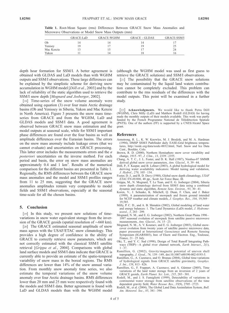
depth hoar formation for SSM/I. A better agreement isobtained with GLDAS and LaD models than with WGHMoutputs and SSM/I observations. These large differences canbe explained by the simplistic scheme for deriving snowaccumulation inWGHMmodel [Doll et al., 2003] and by thelack of reliability of the static algorithm used to retrieve theSSM/I snow depth [Mognard and Josberger, 2002].[18] Time-series of the snow volume anomaly were
obtained using equation (3) over four main Arctic drainagebasins (Ob and Yenissey in Siberia, Yukon and Mac Kenziein North America). Figure 3 presents the snow mass time-series from GRACE and from the WGHM, LaD andGLDAS models and SSM/I data. A good agreement isobserved between GRACE snow mass estimation and themodel outputs at seasonal scale, while for SSM/I importantphase differences are found over the four basins as well asamplitude differences over the Eurasian basins. The errorson the snow mass anomaly include leakage errors (that wecannot evaluate) and uncertainties on GRACE processing.This latter error includes the measurements errors and the aposteriori uncertainties on the inverse method. For eachperiod and basin, the error on snow mass anomalies areapproximately 0.4 and 1 km3. Results of the numericalcomparison for the different basins are presented in Table 1.Regionally, the RMS differences between the GRACE snowmass anomalies and the model and SSM/I profiles rangesfrom 11 to 25 mm, suggesting that the GRACE snowanomalies amplitudes remain very comparable to modelfields and SSM/I observations, especially at the seasonaltime-scale for all the chosen basins.
5. Conclusion
[19] In this study, we present new solutions of time-variations in snow water equivalent storage from the inver-sion of the GRACE geoids (spatial resolution of 660 km).[20] The GRACE estimated seasonal amplitude of snow
mass agrees with the USAF/ETAC snow climatology. Thisprovides a high degree of confidence in the ability ofGRACE to correctly retrieve snow parameters, which arenot correctly estimated with the classical SSM/I satelliteretrieval [Grippa et al., 2004]. Comparisons with globalland surface models and SSM/I data indicate that GRACE iscurrently able to provide an estimate of the spatio-temporalvariability of snow mass in the boreal regions. The RMSdifferences are lower than 14% of the snow annual varia-tion. From monthly snow anomaly time series, we alsoestimate the temporal variations of the snow volumeanomaly over four Arctic drainage basins. RMS differenceslower than 20 mm and 25 mm were respectively found withthe models and SSM/I data. Better agreement is found withLaD and GLDAS models than with the WGHM model
(although the WGHM model was used as first guess toretrieve the GRACE solutions) and SSM/I observations.[21] The possibility that the GRACE snow solutions
may be contaminated by the liquid land waters contribu-tion cannot be completely excluded. This problem cancontribute to the rms residuals of the differences with themodel outputs. This point will be examined in a furtherstudy.
[22] Acknowledgments. We would like to thank Petra Doll(WGHM), Chris Milly (LaD) and Matthew Rodell (GLDAS) for havingmade the monthly outputs of their models available. This work was partlyfunded by the French Programme National de Teledetection Spatiale(PNTS). One of the authors (FF) is supported by a CNES/Alcatel Spacegrant.
ReferencesArmstrong, R. L., K. W. Knowles, M. J. Brodzik, and M. A. Hardman(1994), DMSP SSM/I Pathfinder daily EASE-Grid brightness tempera-tures, http://nsidc.org/data/nsidc-0032.html, Natl. Snow and Ice DataCent., Boulder, Colo.
Brown, R. D. (2000), Northern Hemisphere snow cover variability andchange, 1915–97, J. Clim., 13, 2339–2355.
Chang, A. T. C., J. L. Foster, and D. K. Hall (1987), Nimbus-07 SMMRderived global snow cover parameters, Ann. Glaciol., 9, 39–44.
Doll, P., F. Kaspar, and B. Lehner (2003), A global hydrological model forderiving water availability indicators: Model tuning and validation,J. Hydrol., 270, 105–134.
Foster, D. J., and R. D. Davy (1988), Global snow depth climatology, USAFETAC/TN-88/006, 48 pp., Scott Air Force Base, Ill.
Grippa, M., N. Mognard, T. Le Toan, and E. G. Josberger (2004), Siberiasnow depth climatology derived from SSM/I data using a combineddynamic and static algorithm, Remote Sens. Environ., 93, 30–41.
Koren, V., J. Schaake, K. Mitchell, Q. Duan, F. Chen, and J. Baker(1999), A parameterization of snowpack and frozen ground intendedfor NCEP weather and climate models, J. Geophys. Res., 104, 19,569–19,585.
Milly, P. C. D., and A. B. Shmakin (2002), Global modeling of land waterand energy balances: 1. The Land Dynamics (LaD) model, J. Hydrome-teorol., 3, 283–299.
Mognard, N. M., and E. G. Josberger (2002), Northern Great Plains 1996–1997 seasonal evolution of snowpack from satellite passive microwavemeasurements, Ann. Glaciol., 34, 15–23.
Mognard, N. M., A. V. Kouraev, and E. G. Josberger (2003), Global snow-cover evolution from twenty years of satellite passive microwave data,paper presented at International Geoscience and Remote SensingSymposium (IGARSS03), Inst. of Electr. and Electron. Eng., Toulouse,France, 21–25 July.
Oki, T., and Y. C. Sud (1998), Design of Total Runoff Integrating Path-ways (TRIP)—A global river channel network, Earth Interact., 2(1),1–37.
Ramillien, G. (2002), Gravity/magnetic potential of uneven shelltopography, J. Geod., 76, 139–149, doi:10.1007/s00190-002-0193-5.
Ramillien, G., A. Cazenave, and O. Brunau (2004), Global time-variationsof hydrological signals from GRACE satellite gravimetry, Geophys.J. Int., 158, 813–826.
Ramillien, G., F. Frappart, A. Cazenave, and A. Guntner (2005), Timevariations of the land water storage from an inversion of 2 years ofGRACE geoids, Earth Planet. Sci. Lett., 235, 283–301.
Rodell, M., and J. S. Famiglietti (1999), Detectability of variations incontinental water storage from satellite observations of the timedependent gravity field, Water Resour. Res., 35(9), 2705–2723.
Rodell, M., et al. (2004), The Global Land Data Assimilation System, Bull.Am. Meteorol. Soc., 85, 381–394.
Table 1. Root-Mean Square (rms) Differences Between GRACE Snow Mass Anomalies and
Microwave Observations or Model Snow Mass Outputs (mm)
GRACE-LaD GRACE-WGHM GRACE - GLDAS GRACE-SSM/I
Ob 14 14 14 17Yenisey 19 17 19 25Mac Kenzie 13 15 17 24Yukon 11 14 18 16
L02501 FRAPPART ET AL.: SNOW MASS GRACE L02501
4 of 5

Swenson, S., J. Wahr, and P. C. D. Milly (2003), Estimated accuracies ofregional water storage variations inferred from the Gravity Recoveryand Climate Experiment (GRACE), Water Resour. Res., 39(8), 1223,doi:10.1029/2002WR001808.
Tapley, B. D., S. Bettadpur, M. Watkins, and C. Reigber (2004a), TheGravity Recovery and Climate Experiment: Mission overview and earlyresults, Geophys. Res. Lett., 31, L09607, doi:10.1029/2004GL019920.
Tapley, B. D., S. Bettadpur, J. C. Ries, P. F. Thompson, and M. Watkins(2004b), GRACE measurements of mass variability in the Earth system,Science, 305, 503–505.
Wahr, J., and M. Molenaar (1998), Time variability of the Earth’s gravityfield: Hydrological and oceanic effects and their possible detection usingGRACE, J. Geophys. Res., 103(B12), 30,205–30,229.
S. Biancamaria, A. Cazenave, F. Frappart, N. M. Mognard, andG. Ramillien, Laboratoire d’Etudes en Geophysique et OceanographieSpatiales, UMR 5566, CNES/CNRS/IRD/UPS, 14 Av. Edouard Belin,F-31400 Toulouse, France. ([email protected])
L02501 FRAPPART ET AL.: SNOW MASS GRACE L02501
5 of 5

Hydrologie spatiale : Développement d’outils méthodologiques pour l’utilisation de la télédétection sur les
grands bassins fluviaux
Chapitre 7 : GRACE et l’hydrologie continentale
179
5.4 Estimation de l’évapotranspiration à l’échelle du basin versant
L’évolution du taux d’évapotranspiration (ET), variable utilisée comme conditions aux limites
pour les modèles de climat, fournit de précieuses indications sur les changements climatiques.
L’estimation précise de ce paramètre hydrologique est nécessaire pour une meilleure
compréhension du cycle de l’eau sur Terre. Il n’existe, à l’heure actuelle, aucun réseau
mondial, ni même régional, de mesure d’ET à la surface de la planète. Dans les modèles
hydrologiques globaux, ET est modélisée suivant différentes approches empiriques comme
l’équation de Penman [de Marsily, 1981], par la paramétrisation du flux de chaleur latente
[Ducoudré et al., 1993; Milly et Shmakin, 2002], au moyen de la bulk equation introduite par
Monteith [1963].
A l’échelle régionale, les variations temporelles d’ET sont fonction des conditions
climatiques, de l’humidité des sols, du type de couvert végétal et des surfaces en eau (lacs,
rivières, zones inondées). Ces conditions de surface étant assez mal connues, les modèles
existants fournissent des estimations d’ET assez dissemblables, tant mensuellement qu’à
l’échelle interannuelle [Verant et al., 2004].
La résolution de l’équation de bilan hydrique permet l’estimation de l’évapotranspiration à
l’échelle du bassin versant:
RETPt
W −−=∆∆
(Eq. 7-3)
où t
W
∆∆
est la variation de masse d’eau ∆W pendant l’intervalle de temps ∆t, P et ET, les taux
de précipitation et d’évapotranspiration et R le ruissellement.
Des comparaisons avec les sorties de différents modèles hydrologiques globaux (WGHM,
LaD, GLDAS et ORCHIDEE) témoignent d’un bon accord à l’échelle de grands bassins
versants (Figure 7-8).

Hydrologie spatiale : Développement d’outils méthodologiques pour l’utilisation de la télédétection sur les
grands bassins fluviaux
Chapitre 7 : GRACE et l’hydrologie continentale
180
Figure 7-8: Comparaison des ET déduites de GRACE et estimées par différents modèles globaux de
surface. En noir GRACE, en bleu GLDAS, en rouge LaD, en vert WGHM, en violet ORCHIDEE.

Hydrologie spatiale : Développement d’outils méthodologiques pour l’utilisation de la télédétection sur les
grands bassins fluviaux
Chapitre 7 : GRACE et l’hydrologie continentale
181
Mapping time-variations of evapotranspiration rate from GRACE satellite gravimetry
G. Ramillien1, F. Frappart
1, A. Güntner
2, T. Ngo-Duc
3 and A. Cazenave
1
1 LEGOS, CNES/CNRS UMR5566, Observatoire Midi-Pyrénées, Toulouse, France
2 Engineering Hydrology, GeoForschungZentrum (GFZ), Telegrafenberg, Potsdam, Germany
3 IPSL/Laboratoire de Météorologie Dynamique (LMD), Paris, France
Submitted to Water Resources Research, June 2005
En révision
Corresponding address:
G. Ramillien
GOHS, LEGOS UMR5566 - OMP
18, Avenue Edouard Belin
31400 Toulouse, France
Tel: (+33) 05 61 33 29 34
e-mail: [email protected]
Hydrologie spatiale : Développement d’outils méthodologiques pour l’utilisation de la télédétection sur les
grands bassins fluviaux
Chapitre 7 : GRACE et l’hydrologie continentale
182
Abstract
Since its launch in March 2002, the GRACE mission currently measures the global time
variations of the Earth’s gravity field with a current resolution of ~500 km. Especially over
the continents, these measurements represent the integrated effects of all the water mass
including surface waters (wetlands and rivers), soil moisture, groundwater and snow cover.
We used the GRACE land waters solutions, previously extracted from the available series of
monthly geoids (from April 2002 to May 2004) using an iterative inverse method (Ramillien
et al., 2005a), to estimate monthly maps of evapotranspiration rates -and associated
uncertainties- by integrating and solving the water mass balance equation, which relates land
water storage (from GRACE), precipitation data (from Global Precipitation Climatology
Centre), runoff (from a global land surface model) and evapotranspiration (the unknown).
Results were confronted to outputs from four different global land surface models. Seasonal
cycle and Orthogonal Empirical Function (EOF) analyses of the GRACE-derived
evapotranspiration maps were performed to characterize the global evolution of this
hydrological parameter.
1. Introduction
Evolution of evapotranspiration (ET) provides precious indications of climate change, as well
as important boundary conditions for climate models. Quantification of this hydrological
parameter contributes to a better understanding of the water cycle on Earth. Unfortunately,
there is no complete regional and/or global measurement of ET on the surface of our planet.
In global land surface models, ET is modelled through different empirical approaches, e.g.,
using the Penman equation (De Marsily, 1981), through parameterization of the latent heat
flux (Ducoudré et al., 1993, Milly and Shmakin, 2002) according to the bulk equation
introduced by Monteith (1963), etc. At large scales, the temporal distribution of ET is a
function of climatic conditions, soil moisture availability, the vegetation type as well as the
area of the surface water (wetlands and rivers). These surface conditions are poorly known for
global scale modelling. Existing models provide substantially dissimilar estimates at monthly,
seasonal and even annual time scales (Verant et al., 2004).
First results of previous studies on monthly GRACE (Gravity Recovery and Climate
Experiment) geoids (Tapley et al., 2004; Wahr et al., 2004; Schmidt et al., 2005, Ramillien et
al., 2005a) suggest that the variations continental water storage are mainly seasonal and the
largest amplitudes are located in the large tropical basins of Africa and South America, in the

Hydrologie spatiale : Développement d’outils méthodologiques pour l’utilisation de la télédétection sur les
grands bassins fluviaux
Chapitre 7 : GRACE et l’hydrologie continentale
183
South East Asia during monsoon events, as well as in the high-latitude regions of the
Northern hemisphere due to the snow. These patterns are consistent with those provided by
global land surface models, such as the Water GAP Global Hydrology Model (WGHM; Döll
et al., 2003), the Land Dynamics model (LaD; Milly and Shmakin, 2002), the Global Land
Data Assimilation System (GLDAS; Rodell et al., 2004a), Organizing Carbon and Hydrology
In Dynamics EcosystEms model (ORCHIDEE; Verant et al., 2004). Rodell et al. (2004b)
computed time-series of ET over the Mississippi River basin, using the land water
information from the monthly GRACE geoids combined with precipitation and runoff data.
Rodell et al. (2004b) showed that the GRACE-derived ET is comparable to the estimates
provided by the ECMWF (European Center for Medium range Weather Forecasting)
reanalysis and the GLDAS models.
In this paper, we present a method to compute global maps of ET rate (and associated
uncertainties) by integrating versus time, and then solving, the water mass equation using land
water solutions derived from GRACE (Ramillien et al., 2005a) and independent information
for precipitation observations and runoff model forecasts. We present monthly maps of ET
over lands from April 2002 up to May 2004. For validation, we compared our global
predictions of ET rate with existing model maps. Seasonal analysis and EOF decomposition
of the ET maps and residuals are also performed to characterize the ET changes. We compute
time-series of ET in eight large basins using these monthly solutions as well.
2. Method
The general form of the water mass balance equation is:
RETt
WP ++∆
∆= (1)
where the terms P and ET represent the vertical fluxes (i.e., precipitation and evapo-
transpiration rate respectively). ∆W/∆t and R are the water mass storage variation ∆W during
the period of time ∆t, and the runoff respectively. These terms are generally expressed in
terms of water mass (mm of equivalent-water height) or pressure (kg/m2) per month.
A surface density function F(θ, λ, t) that represents the global map of P, ET, R or W and
depends upon co-latitude θ, longitude λ and time t can be expanded in surface spherical
harmonic coefficients to a maximum degree N:
[ ] )(cos)sin()()cos()(),,(1 0
θλλλθ nm
N
n
n
m
F
nm
F
nm PmtSmtCtF ∑∑= =+= (2)

Hydrologie spatiale : Développement d’outils méthodologiques pour l’utilisation de la télédétection sur les
grands bassins fluviaux
Chapitre 7 : GRACE et l’hydrologie continentale
184
where n and m are the degree and order respectively, Pnm is the associated Legendre function,
and CnmF(t) and Snm
F(t) are the normalized coefficients of the decomposition (units: mm of
equivalent-water thickness).
By isolating the ET term in Eq.1 and considering the spherical analysis from Eq.2, the
coefficients of the ET rate for a given period t )( 21 ttt ≤≤ can be simply evaluated by:
( )12
12
12 /)()(
)()(
)(
)(
)(
)(
)(
)(tt
tStS
tCtC
tS
tC
tS
tC
tS
tCW
nm
W
nm
W
nm
W
nm
R
nm
R
nm
P
nm
P
nm
ET
nm
ET
nm −
−−−
−
=
(3)
Synthesis of these coefficients (Eq.3) provides the corresponding global map of ET(θ, λ, t). In
practice, the lap of time ∆t=t2 - t1 is typically of ~1 month.
As Eq.1 is linear, one can derive easily the associated absolute errors on the computed ET
values from the relative uncertainties Pε and Rε on P and R respectively:
++≈ RP
W
EtW
tETt εελθσλθλθσ
),,(2),,(),,( (4)
where W(θ, λ, t) is the variations of the water mass storage (i.e., the land waters solution from
GRACE) for the month t, and Wσ is the total error for a single month GRACE solution.
Relative uncertainty on precipitation fields Pε was estimated at ~11% according to Rodell et
al. (2004b). A realistic value of ~5% can be chosen for the runoff forecasts (Dingman, 2001).
Wahr et al., (2004) estimated Wσ to be ~18 mm for a 750-km spatial averaging of the
GRACE data. Ramillien et al. (2005b) found Wσ ~15 mm for the GRACE-derived land water
solutions.
3. Data used in this study
3.1 The land water solutions estimated from GRACE
As presented in Ramillien et al. (2005a), the land water solutions consist of spherical
harmonic coefficients of the total water mass (surface waters: rivers, lakes, flood plains; soil
moisture; groundwater; snow) on the continents. These monthly coefficients have been are
truncated at degree 30 (i.e., spatial resolution of ~660 km) because of the current noise of
higher degree coefficients (see for example Tapley et al., 2004, Schmidt et al., 2005). We
used 22 GFZ (GeoForschungZentrum, Potsdam, Germany) and CSR (Center for Space
Research, Austin, Texas) monthly GRACE geoids, from April 2002 to May (2004) –note that
a few monthly geoids are unavailable- and derived monthly solutions of total land water
storage using an iterative inverse method (Ramillien et al., 2005a). Computation of monthly

Hydrologie spatiale : Développement d’outils méthodologiques pour l’utilisation de la télédétection sur les
grands bassins fluviaux
Chapitre 7 : GRACE et l’hydrologie continentale
185
land water solutions consists of improving iteratively the input coefficients (“first guess”) of a
global land surface model (e.g., WGHM), and using the GRACE observations as constraints
(Ramillien et al., 2004). The coefficients were converted into surface density function
coefficients (expressed in mm of equivalent water thickness) by linear filtering (Wahr et al.
1998; Ramillien, 2002) that takes elastic compensation of the Earth’s surface into account.
Associated a posteriori uncertainties on the estimated land water coefficients were also
computed.
3.2 Other data sets used in this study for the period 2002-2004
3.2.a The precipitation rate (GPCC)
The monthly Global Precipitation Climatology Centre (GPCC) products (Rudolf et al., 1994)
are gridded data sets based on raingauge observations, which have been checked using a high
level quality control system (Rudolf et al., 2003). We used the products with the 1° by 1°
geographical latitude and longitude resolution that contain monthly precipitation totals
(mm/month) derived from records of 30,000 to 40,000 gauge stations.
3.2.b The runoff from WGHM
For runoff, we used the predicted values from WGHM (Döll et al., 2003). WGHM was
specifically designed to estimate river discharge for water resources assessments. It computes
0.5°x0.5° gridded time series of monthly runoff and river discharge and is tuned against time
series of annual rivers discharges measured at 724 globally distributed stations. The runoff
from the land surface is computed in soil water balance of the model that takes into account
the water content within the effective root zone, the effective precipitation and the ET. This
vertical water balance of the land and open water fraction of each cell is coupled to a lateral
transport scheme, which routes the runoff through series of storages within the cell and then
transfers the resulting cell outflow to the downstream cell. It is assumed that
surface/subsurface runoff is routed to surface storage without delay. Other products of the
model are monthly gridded time series of snow depth, soil water within the root zone, ground
water and surface water storage in rivers, lakes and wetlands, ET.
3.3 ET predictions from four different land surface models
Our results for ET rate will be compared to global land surface model predictions. We present
below how this hydrological parameter is computed by these models.

Hydrologie spatiale : Développement d’outils méthodologiques pour l’utilisation de la télédétection sur les
grands bassins fluviaux
Chapitre 7 : GRACE et l’hydrologie continentale
186
3.3.a ET prediction from WGHM
The ET from WGHM is computed as a function of potential ET (the difference between the
maximum potential ET and the canopy transpiration), the soil water content in the effective
root zone and the total available soil capacity as:
( )
−−=max
max,mins
scpotcpot
S
SEEEEET (5)
where: ET is the evapotranspiration (mm/day), Epot is the potential ET (mm/day), Ec is the
evaporation from the canopy (mm/day), Epot max is the maximum potential ET (mm/day), Ss is
the soil water content within the effective root zone (mm), Ss max is the total available soil
water capacity within the effective root zone (mm). These 1° x 1° gridded monthly data are
available for 2002 to 2004.
3.3.b ET predictions from LaD
The LaD model (Milly and Shmakin, 2002) provides monthly 1° x 1° gridded time series of
surface parameters estimated from January 1980 to April 2004. For each cell of the model,
the total water storage is composed of three stores: a snowpack store, a root-zone store and a
groundwater store and the total energy storage is equal to the sum of latent heat of fusion of
the snowpack and the glacier and sensible heat content. ET is parameterized as:
( )( )
−+= 1,75.0
min*0
R
Ras
sa
a
W
WqTq
rrET
ρ (6)
where: ρa is the density of the air, ra is the aerodynamic resistance for scalar transfer, rs is a
bulk stomatal resistance under conditions of negligible water stress, qs(T0) is the mixing ratio
of water vapour associated with saturated conditions at the surface temperature, qa is the
mixing ratio at a given level in the atmospheric surface layer, WR is the water storage in the
root-zone store, WR* is the maximum possible value of WR. The final factor in Eq.6 accounts
for the limitation of ET by water stress.
3.3.c ET predictions from GLDAS
The GLDAS project is led by scientists of the National Aeronautics and Space Administration
(NASA) and the National Oceanic and Atmospheric Administration (NOAA) in association

Hydrologie spatiale : Développement d’outils méthodologiques pour l’utilisation de la télédétection sur les
grands bassins fluviaux
Chapitre 7 : GRACE et l’hydrologie continentale
187
with researchers of the Princeton University, the University of Washington and the Weather
Service Office of Hydrology (Rodell et al., 2004a). This uncoupled land surface model which
is used in climate analysis is forced by real time outputs of the NCEP reanalysis, satellite data
and radar precipitation measurements. Parameters are deduced from high-resolution
vegetation, soil coverage and ground elevation data. Data assimilation is performed by one-
dimensional Kalman filtering strategy to produce optimal fields of surface parameters.
Nominal spatial and temporal resolutions of the grids are 0.25 degree and 3 hours
respectively, and all the fields are defined for all land north of -60 deg. Monthly 1°x1° means
of the ET rates (units: kg/m2) were interpolated from these nominal 3-hour outputs. Due to
problems of simulation in the ET subroutine of GLDAS, the ET rate fields after 10/2002 were
computed as the ratio of the predicted latent heat flux and the constant latent heat of
evaporation (around 2.501 106 J/kg).
3.3.d ET predictions from ORCHIDEE
The ORCHIDEE land surface model (Verant et al., 2004; Krinner et al., 2005), developed at
the Institut Pierre Simon Laplace, provides monthly 1° x 1° gridded time series of surface
parameters estimated from 1948 to 2003. For this study, we have only used the ET output of
SECHIBA (Schématisation des Echanges Hydriques l’Interface entre la Biosphère et
l’Atmosphère) (Ducoudré et al., 1993; De Rosnay and Polcher, 1998), which is the water and
energy cycle component of ORCHIDEE. In SECHIBA, the ET flux is described using the
bulk equation introduced by Monteith (1963), similar to Eq.6.
4. Results
For estimating E using Eq.1, one could compute the difference between two successive land
water solutions from GRACE. However, since the GRACE-derived land water solutions are
provided as series of harmonic coefficients of geoid anomaly converted into water mass,
gridded values of P and R have to be developed in terms of spherical harmonic analysis, and
then filtered at degree 30 to remain consistent with and the spatial resolution of the land water
grids. For this purpose, each monthly map provided by the GPCC precipitation data set and
WGHM-based runoff was expanded in spherical harmonic coefficients that are defined in
Eq.2, up to the maximum degree N=100. We computed the ET rate coefficients for each
month from April 2002 to July 2004 by applying Eq.3. In a next step, spherical harmonic
coefficients of ET were transformed into global 1°x1° grids. For deriving a complete series of
monthly maps of ET rate, we interpolated linearly the GRACE land water coefficients for the

Hydrologie spatiale : Développement d’outils méthodologiques pour l’utilisation de la télédétection sur les
grands bassins fluviaux
Chapitre 7 : GRACE et l’hydrologie continentale
188
missing months (i.e., June, July and December 2002 as well as January 2004) before using
Eq.3. The ET maps were divided by a factor of ~30 to convert them into mm per day.
In the following, we present the rms differences between the estimated ET rates from this
study and the ones provided by the four available land surface models (GLDAS, WGHM,
LaD and ORCHIDEE). Large regional rms differences (1.5 – 1.6 mm/day) exist in tropical
basins, and over the Labrador region for all the models. In this latter region, the important rms
differences can be explained by a too simplistic modelling of the snow accumulation from the
models. In other regions, the amplitudes of the rms difference in the tropical basins are
relatively low compared to the amplitudes of the ET signals.
The time series of the rms differences on the continents versus time are plotted on Fig. 3, the
values remain less than 0.8 - 1 mm/day, with a peak of 1.0-1.1 mm/day amplitude during
Spring 2003 for the four models, suggesting important errors from the GRACE land water
solutions during this period. It is also shown on Fig.3 that WGHM, GLDAS and ORCHIDEE
are statistically closer to GRACE-based ET values than LaD.
5. Deriving time-series of ET rate in large drainage basins
For each month, we have spatially averaged the ET values over eight river basins: Amazon,
Congo, Mississippi, Niger, Yangtze-Kiang, Ganges, Brahmaputra and Mekong. The mean
geographical value of ET inside a basin of area S and for the period t can be simply computed
by using the following formula of summation:
∑∈=Sj
jjj
e tES
RtE θδθδλλθ sin),,()(
2
(7)
where δλ and δθ are the grid steps in longitude and latitude respectively (generally δλ=δθ),
and Re the mean radius of the Earth (~6378 km).
For a given month t, the corresponding variation of water volume per day ∆VET is given by
(Ramillien et al., 2005a):
)(sin),,()( 2 tEStERtVSj
jjjeET ×==∆ ∑∈ θδθδλλθ (8)
For each drainage basin, the gridded ET values were extracted using a one-degree mask,
which was computed from the geographical coordinates of the basin boundaries. The
predicted time series of the ET rate are compared to the ET rate computed from the GLDAS,
WGHM, LaD and ORCHIDEE models (Fig 1). Results of the numerical comparison per basin
are presented in Table 1. Regionally, the rms differences between the GRACE ET time series
and the model ET profiles ranges from 0.27 to 0.78 mm/day, suggesting that the GRACE-

Hydrologie spatiale : Développement d’outils méthodologiques pour l’utilisation de la télédétection sur les
grands bassins fluviaux
Chapitre 7 : GRACE et l’hydrologie continentale
189
derived ET amplitudes are in agreement with the values provided by the models, especially at
the seasonal scale for all the chosen basins, except the Amazon (i.e., peak of the GRACE-
based ET rate at the beginning of 2004).
In particular, our results for the Mississippi basin are very comparable with those obtained
previously by Rodell et al. (2004b) for the Mississippi basin. These authors derived a time-
series of the ET rate changes by low-pass filtering the GRACE geoids according to the Wahr
et al., (1998) method. They also found a good agreement with the GLDAS model for monthly
means (~0.83 mm/day rms) at the spatial resolution of 750 km. 0.3-0.8 mm/day is the typical
range of rms differences between GRACE-based ET and model ET we found for the eight
drainage basins that we chose. We found the best agreement between GRACE-based land
model and model forecasts for the Mississippi basin (0.3–0.4 mm/day rms). As this basin is
well-covered by the field observations, this particular comparison reinforces efficiently the
validation of our GRACE-based ET solutions.
7. Summary
In this study, we developed an approach based on the resolution of the water mass balance
equation to derive the global time variations of the ET rate from satellite data of the GRACE
mission. This method enabled us to compute successfully the monthly ET maps for the 2-year
GRACE period (2002-2004) that reveal to be realistic global time-variations of the ET rate.
We also computed the associated absolute errors on the monthly estimates of ET from the
knowledge of relative uncertainties on the precipitation and the runoff. Comparison of the
GRACE-derived ET solutions with different global model outputs shows a good agreement,
especially at the seasonal scale.
In the future, the series by new GRACE land water solutions as input to the proposed
approach to complete the series of ET rate maps. New perspectives of ET rate estimation from
space gravimetry would give access to further surface information such as vegetation
distribution and soil type.
Acknowledgements
We would like to thank Petra Döll, Chris Milly, Matthew Rodell and K. Laval for having
made the monthly outputs of their models available to us. This work was partly funded by the
French Programme National de Télédection Spatiale (PNTS). One of us (FF) benefited from a
CNES-ALCATEL SPACE PhD grant.

Hydrologie spatiale : Développement d’outils méthodologiques pour l’utilisation de la télédétection sur les
grands bassins fluviaux
Chapitre 7 : GRACE et l’hydrologie continentale
190
References
De Marsily G., 1981, Hydrologie quantitative, Ed. Masson, Paris, In French, ISBN: 2-225-
75504-3, 217 pp.
De Rosnay P. and J. Polcher, 1998, “Modeling root water uptake in a complex land surface
scheme coupled to a GCM”, Hydrology and Earth System Sciences, 2(2-3), 239-256.
Dingman S. L., 2001, Physical Hydrology, Prentice-Hall, Englewood Cliffs, N.J, ISBN: 0-
13-099696-5, pp. 646.
Döll P., F. Kaspar and B. Lehner, 2003, “A global hydrological model for deriving water
availability indicators: model tuning and validation”, J. Hydrol., 270, 105-134.
Ducoudré N., K. Laval and A. Perrier, 1993, “SECHIBA: a new set of parametrization of the
hydrologic exchanges at the land/atmosphere interface within the LMD atmosphere general
circulation model”, J. Climate, 6 (2), 248-273.
Krinner G., N. Viovy, N. De-Noblet-Ducoudré, J. Ogée, J. Polcher, P. Friedlingstein, P. Ciais,
S. Sitch and C. Prentice, 2005, “A dynamic global vegetation model for studies of the coupled
atmosphere-biosphere system”, Global Change Biology, 19, GB1015, doi:
10.1029/2003GB002199.
Milly P. C. D. and A. B. Shmakin, 2002, “Global modelling of land water and energy
balances: 1.The Land Dynamics (LaD) model”, J. Hydrometeorol., 3, 283-299.
Monteith J. L., 1963, “Gas exchange in plant communities”, Environmental Control of Plant
Growth, L. T. Evans, Ed. Academic Press, 95-112.
Ramillien G., 2002, “Gravity/magnetic potential of uneven shell topography”, J. of Geodesy,
76, 3, ISSN: 0949-7714, 139-149.

Hydrologie spatiale : Développement d’outils méthodologiques pour l’utilisation de la télédétection sur les
grands bassins fluviaux
Chapitre 7 : GRACE et l’hydrologie continentale
191
Ramillien G., A. Cazenave and O. Brunau, 2004, “Global time variations of hydrological
signals from GRACE satellite gravimetry”, Geophys. J. Int., 158, 813-826.
Ramillien G., F. Frappart, A. Cazenave and A. Güntner, 2005a, “Time variations of the land
water storage from an inversion of 2 years of GRACE geoids”, EPSL, in publication.
Ramillien G., A. Cazenave, Ch. Reigber, R. Schmidt and P. Schwintzer, 2005b, “Recovery of
global time variations of surface water mass by GRACE geoid inversion”, IAG meeting
Proceedings, Springer-Verlag, Porto, Portugal.
Rodell M. and J. S. Famiglietti, 1999, “Detectability of variations in continental water storage
from satellite observations of the time dependent gravity field”, Water Resour. Res., 35, 2705-
2723.
Rodell M. et al., 2004a, “The Global Land Data Assimilation System”, Bull. Am. Meteorol.
Soc., 85, 381-394.
Rodell M., J. S. Famiglietti, J. Chen, S. I. Seneviratne, P. Viterbo, S. Holl and C. R. Wilson,
2004b, “Basin scale estimate of evapotranspiration using GRACE and other observations”,
Geophys. Res. Lett., 31, L20504, doi: 10.1029/2004GL020873.
Rudolf, B., H. Hauschild, W. Rueth and U. Schneider, Terrestrial Precipitation Analysis:
Operational Method and Required Density of Point Measurements. In: Global Precipitations
and Climate Change (Ed. M. Desbois, F. Desalmond), NATO ASI Series I, Vol. 26, Springer-
Verlag, p. 173-186, 1994.
Rudolf, B., T. Fuchs, U. Schneider and A. Meyer-Christoffer, Introduction of the Global
Precipitation Climatology Centre (GPCC), Deutscher Wetterdienst, Offenbach a.M.; pp. 16.,
2003.
Schmidt R., F. Flechtner, Ch. Reigber, P. Schwintzer, A. Güntner, P. Döll, G. Ramillien, A.
Cazenave, S. Petrovic, H. Jochman and J. Wunsch, 2005, “GRACE observations of changes
in continental water storage”, Glob. And Plan. Change, in press.

Hydrologie spatiale : Développement d’outils méthodologiques pour l’utilisation de la télédétection sur les
grands bassins fluviaux
Chapitre 7 : GRACE et l’hydrologie continentale
192
Tapley B. D., S. Bettadpur, M. Watkins and Ch. Reigber (2004). The Gravity Recovery and
Climate Experiment: mission overview and early results, Geophys. Res. Lett., L09607, doi:
10.1029/2004GL019920.
Toumazou V. and J.-F. Crétaux, 2001, “Using a Lanczos eigensolver in the computation of
Empirical Orthogonal Functions”, Monthly Weather Review, 129, 5, 1243-1250, doi:
10.1175/1520-0493.
Verant S., K. Laval, J. Polcher and M. Castro, 2004, “Sensitivity of the continental
hydrological cycle to spatial resolution over the Iberian Peninsula”, J. of Hydrometeo., 5(2),
267-285.
Wahr J., M. Molenaar and F. Bryan, 1998, “Time-variability of the Earth’s gravity field:
hydrological and oceanic effects and their possible detection using GRACE”, J. Geophys.
Res., 103, 30,205-30,230.
Wahr J., S. Swenson, V. Zlotnicki and I. Velicogna, 2004, “Time-variable gravity from
GRACE: first results”, Geophys. Res. Lett., 31, L11501, doi: 10.1029/2004GL019779.

Hydrologie spatiale : Développement d’outils méthodologiques pour l’utilisation de la télédétection sur les
grands bassins fluviaux
Chapitre 7 : GRACE et l’hydrologie continentale
193
Table 1
Regional root-mean square (rms) differences between GRACE-derived ET solutions and model ET forecasts:
geographical ET means per basin (units: mm/day).
GRACE-
ORCHIDEE
GRACE-GLDAS GRACE-LaD GRACE-WGHM
Amazon 0.42 0.73 0.60 0.57
Congo 0.45 0.44 0.52 0.45
Mississippi 0.27 0.28 0.36 0.44
Niger 0.46 0.43 0.63 0.40
Yangtze-Kiang 0.49 0.32 0.36 0.64
Ganges 0.62 0.67 0.78 0.56
Brahmaputra 0.61 0.58 0.61 0.59
Mekong 0.69 0.52 0.44 0.56

Hydrologie spatiale : Développement d’outils méthodologiques pour l’utilisation de la télédétection sur les
grands bassins fluviaux
Chapitre 7 : GRACE et l’hydrologie continentale
194
Figure caption
Figure 1: Regional time series of mean ET rate in eight drainage basins of the globe: Amazon, Congo,
Mississippi, Niger, Yangtze-Kiang, Ganges, Brahmaputra, Mekong: GRACE-derived ET rate variations (black
line); GLDAS (blue line); LaD (red line); WGHM (green line) and ORCHIDEE (purple line). See Table 1 for the
statistical results of the comparison per basin.

Hydrologie spatiale : Développement d’outils méthodologiques pour l’utilisation de la télédétection sur les
grands bassins fluviaux
Chapitre 7 : GRACE et l’hydrologie continentale
195
Figure 5

Hydrologie spatiale : Développement d’outils méthodologiques pour l’utilisation de la télédétection sur les
grands bassins fluviaux
Chapitre 7 : GRACE et l’hydrologie continentale
196
6. Discussion – Perspectives
La confrontation des solutions mensuelles « eaux liquides », neige et évapotranspiration avec
les sorties de différents modèles hydrologiques globaux indique que les estimations de la
méthode inverse sont réalistes, tant à l’échelle globale que régionalement. La principale
limitation à l’utilisation des mesures GRACE pour l’hydrologie continentale provient de la
faible résolution spatiale des géoïdes, due à la présence de bruit aux hautes fréquences.
L’amélioration de la qualité des géoïdes mensuels est une priorité des responsables de la
mission GRACE et des équipes souhaitant utiliser cette source de données pour l’hydrologie
continentale. Des géoïdes ayant une meilleure résolution spatiale (~400 km) ont déjà été
obtenus, en utilisant une méthode locale de perturbation du géopotentiel, sur le bassin
amazonien [Han et al., 2005]. L’équipe allemande du GFZ, en charge du traitement des
mesures de la mission GRACE, vient de mettre à disposition de la communauté scientifique,
14 géoïdes dont la qualité a été améliorée par une meilleure prise en compte d’effets
géophysiques comme la marée polaire. Ces nouveaux géoïdes ont pu être inversé jusqu’au
degré 50, c’est-à-dire de l’ordre de 500 km, au sein de l’équipe GOHS. Dans le même temps,
le Groupement de Recherche en Géodésie Spatiale (GRGS) vient de produire des géoïdes, de
résolution temporelle égale à 10 jours et d’une qualité égale à ceux du GFZ, à partir des
mesures de la distance inter-satellite et des accéléromètres présents à bord de chacun des deux
satellites. Des études similaires à celles effectuées dans ce chapitre, pourraient être
reproduites à l’échelle des bassins fluviaux avec des solutions de meilleure résolution spatiale.
A l’échelle du bassin versant ou sur de grandes zones d’inondation, les réserves en eau des
nappes phréatiques sont susceptibles d’être estimées par combinaison de données de
télédétection. L’utilisation de l’altimétrie satellitaire, couplée à l’imagerie spatiale, a démontré
ses potentialités pour l’estimation des variations de volume d’eau de surface. Ces variations
de volume d’eau, soustraites au signal hydrologique mesuré par GRACE, donnent accès à
l’évolution des stocks d’eau des nappes. Une estimation des aquifères sur l’ensemble du globe
est envisageable en soustrayant la composante eau de surface fournie par les modèles
hydrologiques globaux au signal de GRACE.

Hydrologie spatiale : Développement d’outils méthodologiques pour l’utilisation de la télédétection sur les
grands bassins fluviaux
Conclusion
197
Conclusion
Le suivi des variations de stock d’eau continentale est primordial pour une meilleure
compréhension du cycle de l’eau à l’échelle régionale et à l’échelle globale. Les mesures in-
situ de ces variations, lorsqu’elles existent, sont très difficiles à obtenir et souvent
inhomogènes. Les techniques de télédétection spatiale, et particulièrement l’altimétrie
satellitaire, représentent un apport majeur pour les études hydrologiques.
Bien qu’initialement développée et optimisée pour l’étude des océans, l’altimétrie radar a été
utilisée avec succès pour l’étude des surfaces continentales, et en particulier sur les surfaces
recouvertes d’eau. En domaine continental, l’utilisation de l’altimétrie satellitaire est plus
délicate que sur les océans et nécessite des précautions accrues au niveau des mesures et de
l’application des corrections.
En effet, les échos radar observés sur les surfaces continentales recouvertes d’eau, différent
grandement de ceux caractéristiques des surfaces océaniques. Il en résulte une perte d’un
grand nombre de données et d’importantes imprécisions sur les niveaux d’eau déduits des
hauteurs altimétriques. Le retraitement des formes d’onde altimétriques, par un algorithme
adapté à la nature des échos radar observés sur les zones humides (fleuves, zones
d’inondation, petits lacs) apparaît indispensable pour accroître le nombre de données valides
et leur précision. Les résultats obtenus avec les mesures de l’altimètre d’ENVISAT (chapitre
4 et annexe 1), mesures retraitées au sol avec l’algorithme « Ice-1 », fournissent de meilleurs
résultats que celles obtenues avec l’algorithme de suivi de bord de T/P. La classification des
formes d’onde altimétriques, présentée au chapitre 3, montre qu’une grande majorité des
échos radar observés sur les zones humides sont quasi-spéculaires (plus ou moins bruités par
les diffusions sur la végétation). Différentes solutions sont envisageables pour améliorer leur
traitement : l’utilisation d’algorithmes de type analytique (comme « Ice-2 ») dont la forme
d’onde modélisé serait quasi-spéculaire, le recours à des techniques utilisées en traitement
d’images (comme l’identification de contours au moyen d’ondelettes) sont envisageables. Ces
solutions sont actuellement à l’étude au LEGOS.
En dépit des limitations présentées au chapitre 3, les mesures altimétriques demeurent
exploitables pour l’hydrologie continentale. Le concept de stations altimétriques, présenté au
chapitre 4, permet la création de réseaux de mesures de niveaux d’eau denses grâce à
l’échantillonnage spatio-temporel des altimètres radar. La mise en place d’un tel réseau sur le
bassin amazonien, en complément du réseau in-situ existant, a suscité l’intérêt de l’agence de

Hydrologie spatiale : Développement d’outils méthodologiques pour l’utilisation de la télédétection sur les
grands bassins fluviaux
Conclusion
198
l’eau brésilienne (ANA). De nouvelles applications hydrologiques de l’altimétrie satellitaire,
donnant accès à des paramètres hydrologiques importants et difficilement mesurables sur le
terrain, ont ainsi vu le jour sur les grands bassins fluviaux.
Des profils hydrologiques du Rio Negro et de ses principaux affluents, l’Uaupes et le Rio
Branco, ont été estimés à partir des données T/P et ENVISAT. Ces profils, et donc les pentes
des cours d’eau qui peuvent en être déduites, sont le reflet d’effets tectoniques, sédimentaires
et climatiques. La connaissance de la pente d’un fleuve trouve son application en hydrologie
locale car elle est nécessaire au calcul des débits, en l’absence de courbe d’étalonnage entre la
hauteur et le débit. L’altimétrie satellitaire a ainsi démontré sa capacité à être utilisée pour des
études hydrodynamiques [León et al., 2006].
Des variations de volume d’eau de surface ont pu être estimées à partir de la synergie entre
altimétrie radar et imagerie satellitaire. Ces études, menées dans les bassins du Rio Negro et
du Mékong, ont mis en évidence la complémentarité entre altimétrie radar et imagerie
satellitaire (multispectral ou radar). Dans le bassin du Rio Negro, la non-linéarité entre surface
inondée et volume d’eau stockée a été démontrée. Des comparaisons entre volumes stockés
pendant la crue et volume écoulé ont permis d’estimer de manière approximative les temps de
résidence de l’eau dans les différents sous-bassins. L’évolution spatio-temporelle des
inondations a pu être suivie dans le bassin du Mékong pour la période 1998-2003. Une
estimation des variations inter-annuelles du volume d’eau de surface stocké dans ce bassin a
pu être réalisée.
Si l’altimétrie satellitaire (et l’imagerie spatiale) renseignent sur les eaux de surface, la
mission de gravimétrie spatiale GRACE, qui mesure les variations du champ de gravité
terrestre causées par les redistributions de masse dans l’enveloppe terrestre, et donc aux
échelles de temps d’un mois à plusieurs années, donne accès aux changements dans les
réserves d’eau continentales. La méthode inverse développée au sein de l’équipe GOHS
permet de séparer les réserves d’eau continentales en quatre composantes : atmosphère,
océan, « eaux liquides » et neige. Une estimation du terme d’évapotranspiration a été réalisée
au moyen de l’équation de bilan hydrique. La comparaison des solutions mensuelles « eaux
liquides », neige et évapotranspiration, issues de l’inversion des géoïdes, avec les sorties de
différents schémas globaux de surface indique que les estimations de la méthode inverse sont
réalistes, tant à l’échelle globale que régionalement. La principale limitation à l’utilisation des
mesures GRACE pour l’hydrologie continentale provient de la faible résolution spatiale des
géoïdes, due à la présence de bruit aux hautes fréquences. Les nouveaux géoïdes fournis par
l’équipe Géodésie Spatiale du laboratoire de Dynamique Terrestre et Planétaire, de meilleures

Hydrologie spatiale : Développement d’outils méthodologiques pour l’utilisation de la télédétection sur les
grands bassins fluviaux
Conclusion
199
résolutions spatiale (~ 400 km) et temporelle (10 jours), vont faciliter le suivi des
redistributions des masses d’eau continentale et leur impact sur l’évolution du niveau de la
mer.
De ces différents travaux, il ressort que les données de télédétection ont un intérêt primordial
pour l’étude du cycle de l’eau sur les continents. La complémentarité existant entre les
différents instruments (altimètres, satellites imageurs, mission de gravimétrie spatiale)
contribue à améliorer notre compréhension de la phase continentale du cycle de l’eau. De
nombreuses perspectives s’ouvrent au terme de cette étude, tant du point de vue de
l’exploitation des données altimétriques que des mesures de GRACE.
Un des grands enjeux pour les années à venir concerne l’assimilation des données de
télédétection dans les modèles hydrologiques, locaux ou globaux, à l’instar de ce qui se fait
actuellement en météorologie et océanographie, aussi bien pour des problématiques
scientifiques que pour des applications opérationnelles. L’assimilation de produits
hydrologiques GRACE, similaires à ceux présentés dans le chapitre 7, ou de débits calculés à
partir de la méthode présentée dans l’annexe 3, dans des schémas globaux de surface,
permettraient de mieux contraindre des réservoirs assez mal connus comme les aquifères, la
neige ou même les eaux de surface. L’assimilation de mesures altimétriques dans les modèles
hydrologiques devrait permettre la modélisation des plaines d’inondation et des bassins
fluviaux.
Pour l’heure, il n’existe aucune mission spécifiquement dédiée à l’hydrologie continentale.
Certaines sont prévues à plus ou moins long terme :
- pour la mesure de l’humidité des sols : SMOS (Soil Moisture and Ocean Salinity) par
l’ESA et Hydros (Hydrospheric States Mission) par la NASA,
- pour la mesure des niveaux d’eau sur les continents : le projet WatER (Water
Elevation Recovery). Ce projet est né d’une volonté commune de scientifiques
européens [Cazenave et al., 2004] et américains [Alsdorf et al., 2003] de voir
développer, par les agences spatiales américaine et européennes, une plateforme
capable de fournir des mesures des niveaux d’eau sur les lacs, les fleuves et les zones
d’inondation, à l’échelle du globe, pour améliorer nos connaissances des eaux
continentales de surface et contribuer à une meilleure gestion des ressources en eau.
Ces nouvelles missions satellitaires, aux objectifs complémentaires, laissent présager de
nombreux progrès dans le domaine de l’hydrologie continentale.

Hydrologie spatiale : Développement d’outils méthodologiques pour l’utilisation de la télédétection sur les
grands bassins fluviaux
Conclusion
200

Hydrologie spatiale : Développement d’outils méthodologiques pour l’utilisation de la télédétection sur les
grands bassins fluviaux
Bibliographie
201
BIBLIOGRAPHIE
Ad Hoc Work Group on Global Water Datasets (2001). Global water data: an endangered
species, EOS Trans., American Geophysical Union, 82, 54-58.
Alabyan A.M., Chalov R.S. (1998). Types of river channel patterns and their natural controls,
Earth Surface Processes and Landforms, 23, 467-474.
Alsdorf D.E., Melack J.M., Dunne T., Mertes L.AK., Hess L. L., Smith L.C. (2000).
Interferometric radar measurements of water level changes on the Amazon floodplain, Nature,
404, 174-177.
Alsdorf D.E., Smith L.C., Melack J.M. (2001). Amazon floodplain water level changes
measured with interferometric SIR-C radar, IEEE Trans. Geosci. Remote Sensing, 39 (2),
423-431.
Alsdorf D.E., Birkett C., Dunne T., Melack J.M., Hess L. (2001). Water level changes in a
large Amazon lake with spaceborne radar interfermetry and altimetry, Geophys. Res. Lett., 28
(14), 2671-2674.
Alsdorf D.E., Lettenmaier D., Vörösmarty C. (2003). The need for global, satellite-based
observations of terrestrial surface waters, EOS Trans. AGU, 84, 29.
Alsdorf D.E. (2003). Water storage of the central Amazon floodplain measured with GIS and
remote sensing imagery, Annals of the Association of American Geographers, 93 (1), 55-66.
Alsdorf D.E., Lettenmaier D.P. (2003). Tracking fresh water from space, Science, 301, 1492-
1494.
Arino O., Dedieu G., Deschamps P. (1991). Determination of satellite land surface
reflectances using METEOSAT and NOAA/AVHRR shortwave channel data, Int. J. Remote
Sensing, 13, 2263-2287.
Arnaud M., Leroy M.,M. (1991). SPOT 4: a new generation of SPOT satellites, ISPRS
Journal of Photogrammetry and Remote Sensing, 46, 205-215.
AVISO (1996). AVISO User Handbook: Merged TOPEX/POSEIDON Products, AVI-NT-02-
101-CN, 3-rd ed, CNES, Toulouse, France, 194 pp.
Bamber J.L. (1994). Ice sheet altimeter processing scheme, Int. J. Remote Sensing, 15 (4),
925-938.
Bates P.H. (2000). A simple raster-based model for flood inundation simulation, Journal of
Hydrology, 236, 54-77.
Beltrán J.R., García-Lucía J., Navarro J. (1994). Edge detection and classification using
Mallat’s wavelet,

Hydrologie spatiale : Développement d’outils méthodologiques pour l’utilisation de la télédétection sur les
grands bassins fluviaux
Bibliographie
202
Beltrán J.R., Beltrán F., Estopañan A. (1998). Multiresolution edge detection and
classification: noise characterization, Proc. 1998 IEEE Conf. On Systems, Man and
Cybernetics, La Jolla (USA), Oct. 1998, pp. 4476-4481.
Berry P.A.M. (2000). Topography from land radar altimeter data: possibilities and restriction,
Phys. Chem.Earth (A), 25 (1), 81-88.
Berry P. A. M., Garlick J.D., Freeman J.A., Mathers E.L. (2005). Global inland water
monitoring from multi-mission altimetry, Geophys. Res. Lett., 32, L16401,
doi:10.1029/2005GL022814.
Birkett C.M. (1995a). The contribution of TOPEX/POSEIDON to the global monitoring of
climatically sensitive lakes, J. Geophys. Res., 100 (C12), 25,179-25,204.
Birkett C.M. (1995b). The global remote sensing of lakes, wetlands and rivers for
hydrological and climate research, Proc. IGARSS, IEEE, Firenze, July, 1979-1981.
Birkett C.M., Mason, I.M. (1995). A new Global Lakes Database for a remote sensing
programme studying climatically sensitive large lakes, J. of Great Lakes Research, 21(3),
307-318.
Birkett C.M. (1998). Contribution of the TOPEX NASA radar altimeter to the global
monitoring of large rivers and wetlands, Water Resour. Res., 34 (5), 1223-1239.
Birkett C.M., Murtugudde R., Allan T. (1999). Indian Ocean climate event brings floods to
East Africa's lakes and the Sudd marsh, Geophys. Res. Lett., 26(8), 1031-1034., 1999.
Birkett C.M., Mertes L.A.K., Dunne T., Costa M.H., Jasinski M.J. (2002). Surface water
dynamics in the Amazon Basin : Application of satellite radar altimetry, J. Geophys. Res., 107
(D20), 8059-8080.
Bjerklie D.M., Dingman S.L., Vörösmarty C.J., Bolster .H., Congalton R.G. (2003).
Evaluating the potential for measuring river discharge from space, Journal of Hydrology, 278,
17-38.
Bjerklie D.M., Moller D., Smith L.C., Dingman S.L. (2005). Estimating discharge in rivers
using remotely sensed hydraulic information, J. Hydro., 309(1-4), 191-209.
Boon P.J., Davies B.R., Petts G.E. (Eds.) (2000). Global Perspectives on River Conservation :
Science, Policy and Practice, John Wiley & Sons Ltd.
Brakenridge G.R., Knox J.C, Paylor E.D. II, Magilligan F.J. (1994). Radar remote sensing
aids study of the great flood of 1993, EOS Trans. AGU, 75, 521-527.
Brenner A.C., Bindschadler R.A., Thomas R.H., Zwally H.J. (1983). Slope-induced errors in
radar altimetry over continental ice sheets, J. Geophys. Res., 88 (C3), 1617-1623.

Hydrologie spatiale : Développement d’outils méthodologiques pour l’utilisation de la télédétection sur les
grands bassins fluviaux
Bibliographie
203
Brenner A.C., Frey H.V., Di Marzio J., Tsaoussi L. (1997). Topography over South America
from ERS altimetry, Space at the Service of our Environment, ESA Pub. SP-414, 1, May
1997.
Brown G.S. (1977). The average impulse response of a rough surface and is applications,
IEEE Trans. Antennas Propagat., Vol. 25 (1), 67-74.
Brown R.D. (2000). Northern Hemisphere snow cover variability and change, 1915-97, J.
Clim., 13, 2339-2335.
Cartwright D.E., Tayler R.J. (1971). New computations of the tide-generating potential,
Geophys. J. Roy. Astron. Soc., 23, 45-74.
Cartwright D.E., Edden, A.C. (1973). Corrected tables of tidal harmonics, Geophys. J. Roy.
Astron. Soc., 33, 253-264.
Cauduro Dias de Paiva E.M., Clarke R.T. (1996). Time trends in rainfall records in
Amazonia, Bull. Am. Meteorol. Soc., 76, 2203-2211.
Cazenave A., Bonnefond P., Do Minh K. (1997). Caspian sea level from Topex/Poseidon
altimetry: Level now falling, Geophys. Res. Lett., 25 (2), 155-158.
Cazenave A., Milly P.C.D., Douville H., Beneveniste J., Lettenmaier D., Kosuth P. (2004).
International workshop examines the role of space techniques to measure spatio-temporal
change in terrestrial waters, EOS, AGU Trans., 85(6).
Chahine M.T. (1992). The hydrological cycle and its influence on climate, Nature, 359, 373-
380.
Chapman B., Siqueira P., Freeman A. (2002). The JERS Amazon Multi-season Mapping
Study (JAMMS): Observation strategies and data characteristics, Int. J. Remote Sensing, 23
(7), 1427-1446.
Coe M.T., Costa M.H., Botta A., Birkett C.M. (2002). Long term simulations of discharge
and floods in the Amazon Basin, J. Geophys. Res., 107 (D20), 10,129-10,146.
Coe M.T., Birkett C.M. (2004). Calculation of river discharge and prediction of lake height
from satellite radar altimetry for the Lake Chad basin, Water Resour. Res., 40, W10205,
doi:10.129/2003WR002543.
Cosandey C., Robinson M. (2000). Hydrologie continentale, coll. U, Armand Colin, Paris,
360 p.
Costa M.H, Foley J.A. (1997). Water balance of the Amazon Basin: Dependence on
vegetation cover and canopy conductance, J. Geophys. Res., 102 (D20), 23,973-23,989.
Costa M.H, Foley J.A. (1998). A comparison of precipitation datasets for the Amazon basin,
Geophys. Res. Lett., 25 (2), 155-158.

Hydrologie spatiale : Développement d’outils méthodologiques pour l’utilisation de la télédétection sur les
grands bassins fluviaux
Bibliographie
204
Costa M.H, Foley J.A. (1999). Trends in the hydrologic cycle of the Amazon basin, J.
Geophys. Res., 104 (D12), 14,189-14,198.
Costa M.P.F., Niemann O., Novo E., Ahern F. (2002). Biophysical poperties and mapping of
aquatic vegetation during the hydrological cycle of the Amazon floodplain using JERS-1 and
Radarsat, Int. J. Remote Sensing, 23 (7), 1401-1426.
Crétaux J.F., Kouraev A.V., Papa F., Bergé-Nguyen M., Cazenave A., Aladin N., Plotnikov
I.S. (2005). Evolution of sea level of the big Aral Sea from satellite altimetry and its
implications for water balance, J. Great Lakes Res., 31, 520-534.
Cudlip W. (1994). Overview of the altimeter data processing at the U.K. Earth Observation
Data Centre, Int. J. Remote Sensing, 15 (4), 871-887.
Cudlip W., Manntripp D.R., Wrench C.L., Griffiths H.D, Sheehan D.V., Lester M., Leigh
R.P., Robinson T.R. (1994). Corrections for altimeter low-level processing at the Earth
Observation Data Centre, Int. J. Remote Sensing, 15 (4), 889-914.
Dahm C.N., Valett H.M. (1996). Hyporheic zones, in Methods in Stream Ecology, F.R. Hauer
and G.A Lamberti Eds. Academic Press, San Diego, California, 107-119.
Daubechies I. (1990). The wavelet transform, time frequency localization and signal analysis,
IEEE Trans. Inform. Theory, 36 (5), 961-1005.
Dingman S. L. (2001). Physical Hydrology, Prentice-Hall, Englewood Cliffs, N.J, ISBN: 0-
13-099696-5, pp. 646.
Döll P., Kaspar F., Lehner B. (2003). A global hydrological model for deriving water
availability indicators: model tuning and validation, J. Hydrol., 270, 105-134.
Douville H., Chauvin F., Planton S., Royer J.F., Salas-Melia D., Tyteca S. (2002).
Sensitivity of the hydrological cycle to increasing amounts of greenhouse gases and aerosols,
Clim. Dyn., 20, 45-68.
Dow J.M., Martinez Fadrique F.M., Zandbergen R. (1999). High precision altimetry from the
ENVISAT mission, Adv. Space Res., 23 (4), 757-762.
Duchemin B., Berthelot B., Dedieu G., Leroy M., Maisongrande P. (2002). Normalisation of
directional effects in 10-day global syntheses derived from VEGETATION/SPOT : II.
Validation of an operational method on actual datasets, Remote Sens. Env., 81, 101-113.
Ducoudré N., Laval K., Perrier A. (1993). SECHIBA: a new set of parametrization of the
hydrologic exchanges at the land/atmosphere interface within the LMD atmosphere general
circulation model, J. Climate, 6 (2), 248-273.
Dumont J.P. (1985). Estimation optimale des paramètres altimétriques, PhD Thesis, Institut
National Polytechnique de Toulouse.
Dunn C., et al. (2003). Instruments of GRACE: GPS augments gravity measurements, GPS
world, 14(2), 16-28.

Hydrologie spatiale : Développement d’outils méthodologiques pour l’utilisation de la télédétection sur les
grands bassins fluviaux
Bibliographie
205
Eaton B.C., Church M., Millar R.G. (2004). Rational regime model of alluvial channel
morphology and response, Earth Surface Processes and Landforms, 29, 511-529.
Emery W.J., Thomas A.C., Collins M.J., Crawford W.R. Mackas D.L. (1986). An objective
Method for computing advective surface velocities from sequential infrared satellite images,
J. Geophys. Res., 91 (C11), 12,865-12,878.
ESA (2002). ENVISAT RA2/MWR Product Handbook, RA2 /MWR Products User Guide,
353 pp.
Ferguson R.I. (2004). Estimating critical stream power for bedload transport calculations in
gravel-bed rivers, Geomorphology, 70, 33-41.
Fekete B., Vörösmarty C.J., Grabs. W. (1999). Global, Composite Runoff Fields Based on
Observed River Discharge and Simulated Water Balance. Koblenz, Germany: WMO-GRDC.
Foley J.A., Bota A., Coe M.T., Costa M.H. (2002). El Niño-Southern Oscillation and the
climate, ecosystems and rivers of Amazonia, Global Biogeochemical Cycles, 16 (4), 1132-
1151.
Frappart F., Cazenave A., Seyler F., Calmant S. (2005a). Comparison of the ENVISAT
waveform retrackers over inland waters, Proc. of the Envisat & ERS Symposium, Salzburg,
Austria, 6-10 September 2004 (ESA SP-572, April 2005), CD-ROM.
Frappart F., Seyler F., Martinez J.M., León J.G., Cazenave A. (2005b). Floodplain water
storage in the Negro River basin estimated from microwave remote sensing of inundation area
and water levels, Remote Sens. Environ., 99(4), 387-399.
Frappart F., Ramillien G., Biancamaria S., Mognard N.M., Cazenave A. (2006a). Evolution
of high-latitude snow mass derived from the GRACE gravimetry mission (2002-2004),
Geophys. Res. Let., 33(2): L02501, doi:10.1029/2005GL024778.
Frappart F., Calmant S., Cauhopé M., Seyler F., Cazenave A. (2006b). Preliminary results of
ENVISAT RA-2-derived water levels validation over the Amazon basin, Remote Sens.
Environ., 100(2), 252-264.
Frazier P., Page K., Louis J., Briggs S., Robertson A.I. (2003). Relating wetland inundation to
river flow using Landsat TM data, Int. J. Remote Sensing, 24 (19), 3755-3770.
Friborg, T., Soegaard H., Christensen T.R., Lloyd C.R., Panikov N.S. (2003). Siberian
wetlands: Where a sink is a source, Geophys. Res. Lett., 30(21), 2129,
doi:10.1029/2003GL017797.
Fu L.L., Cazenave A. (2001). Satellite altimetry and Earth science, a handbook of techniques
and applications, Academic Press, London, U.K.

Hydrologie spatiale : Développement d’outils méthodologiques pour l’utilisation de la télédétection sur les
grands bassins fluviaux
Bibliographie
206
Gao J., Lythe M.B. (1998). Effectiveness of the MCC method in detecting oceanic circulation
patterns at a local scale from sequential AVHRR images, Photogrammetric Engineering &
Remote Sensing, 301-308.
Gardini B., Graf G., Ratier G. (1995). The instruments on ENVISAT, Acta Astronautica, 37,
301-311.
Grandi G. De, Mayaux P., Rauste Y., Rosenquvist A., Simard M., Saatchi S.S. (2000). The
Global Rain Forest Mapping Project JERS-1 radar mosaic of tropical Africa: development
and product characterization aspects, IEEE Trans. Geosci. Remote Sensing, 38 (5), 2218-
2233.
Guzkowska M.A.J., Rapley C.G., Mason I.M. (1986). Satellite altimeter measurements over
land and inland water, Proceedings of IGARSS’86 Symposium, Zürich, 8-11 Sept. 1986, Ref.
ESA SP-254, 1563-1568.
Guzkowska, M.A.J., Rapley, C.G., Ridley, J.K., Cudlip, W., Birkett, C.M. and Scott, R.F.,
1990. Developments in Inland Water and Land Altimetry, ESA CR-7839/88/F/FL.
Hajj H.M., Nguyen T.Q., Chin R.T. (1996). On multi-scale feature detection using filter
banks, IEEE Trans. Sig. Proc., 1, 70-74.
Hamilton S.K., Sippel S.J., Melack J.M. (1996). Innundation patterns in the Pantanal wetland
of South America determined from passive microwave remote sensing, Arch. Hydrobiol, 137
(1), 1-23.
Hamilton S.K., Souza O.C.de, Couthino M.E. (1998). Dynamics of floodplain innundation in
the alluvial fan of the Taquari River (Pantanal, Brazil), Vehr. Internat. Verein. Limnol., 26,
916-922.
Hamilton S.K. (1999). Potential effects of a major navigation project (Paraguay-Paraná
hidrovía) on inundation in the Pantanal floodplains, Regul. Rivers : Res. Mgmt., 15, 289-299.
Hamilton S.K., Sippel S.J., Melack J.M. (2002). Comparison of innundation patterns among
major South American floodplains, J. Geophys. Res., 107 (D20), 10.129-10.143.
Han S.-C., Shum C.K., Braun A. (2005). High-resolution continental water storage recovery
from low–low satellite-to-satellite tracking, J. Geodynanics, 39(1), 11-28.
Hayne G.S. (1980). Radar altimeter mean return waveforms from near-normal-incidence
ocean surface scattering, IEEE Trans. Antennas Propagat., 28 (5), 687-692.
Hayashi M., van der Kamp G. (2000). Simple equations to represent the volume area depth
relations of shallow wetlands in small topographic depressions, Journal of Hydrology, 237,
74-85.
Hess L.L., Melack J.M., Filoso S., Wang Y. (1995). Delineation of inundated area and
vegetation along the Amazon floodplain with SIR-C synthetic aperture radar, IEEE Trans.
Geosci. Remote Sensing, 33, 896-904.

Hydrologie spatiale : Développement d’outils méthodologiques pour l’utilisation de la télédétection sur les
grands bassins fluviaux
Bibliographie
207
Hess L.L., Melack J.M., Novo E.M.L.M., Barbosa C.C.F., Gastil M. (2003). Dual-season
mapping of wetland inundation and vegetation for the central Amazon basin, Remote Sens.
Environ., 87 (4), 404-428.
Holben B.N. (1986). Characteristics of maximum-value composite images from temporal
AVHRR data, Int. J. Remote Sensing, 7, 1417-1434.
Hori H. (2000). The Mekong environment and development, the United Nations University,
New York USA.
Hsieh J.W., Ko, M.T., Liao H.Y.M., Fan K.C. (1997). A new wavelet-based edge detector via
constrained optimization, Image and Vision Computing, 15, 511-527.
Ilk K.H., Flury J., Rummel R., Schwintzer P., Bosch W., Haas C., Schröter J., Stammer D.,
Zahel W., Miller H., Dietrich R., Huybrechts P., Schmeling H., Wolf D., Riegger J., Bardossy
A., Güntner A. (2005). Mass Transport and Mass Distribution in the Earth System -
Contribution of the New Generation of Satellite Gravity and Altimetry Missions to
Geosciences, Proposal for a German Priority Research Program, GOCE-Projektbüro
Deutschland, Technische Universität München, GeoForschungsZentrum Potsdam, Second
Edition, January 2005.
Interim Mekong Comitee (1988). Perspectives for Mekong Development. Revised indicative
plan (1987) for the development of land, water and related resources of the lower Mekong
basin. Committee report. Interim Committee for Coordination of Investigations of the lower
Mekong Basin, Bangkok, Thailand.
Jensen J.R. (1999). Radar altimeter gate tracking: Theory and extension, IEEE Trans. Geosci.
Remote Sensing, 37 (2), 651-658.
Junk W., Bayley P.B., Sparks R.E, 1989. The flood pulse concept in river floodplain systems,
in D.P. Dodge (Ed.) Proceedings of the International Large River Symposium. (LARS), Can.
Spec. Pub. Fish. Aquat. Sci. 106, 110-127.
Kamachi M. (1989). Advective surface velocities derived from sequential images for
rotational flow field: limitations and applications of maximum cross-correlation method with
rotational registration, J. Geophys. Res., 94 (C12), 18,227-18,233.
Koblinsky C.J., Clarke R.T., Brenner A.C., Frey H. (1993). Measurement of river level
variations with satellite altimetry, Water Resour. Res., 29 (6), 1839-1848.
Kosuth P., Cazenave A. (2002). Développement de l’altimétrie satellitaire radar pour le suivi
hydrologique des plans d’eau continentaux : application au réseau hydrographique de
l’Amazone, Rapport d’activités 2000-2001, Projet PNTS 00/0031/INSU, 39 pp.
Kouraev A., Sakharova E. A., Samain O., Mognard-Campbell N., Cazenave A. (2004). Ob'
river discharge from Topex/Poseidon satellite altimetry, Remote Sens. Environ., 93, 238-245.

Hydrologie spatiale : Développement d’outils méthodologiques pour l’utilisation de la télédétection sur les
grands bassins fluviaux
Bibliographie
208
Krinner G., Viovy N., Noblet-Ducoudré N. de, Ogée J., Polcher J., Friedlingstein P., Ciais P.,
Sitch S., Prentice C. (2005). A dynamic global vegetation model for studies of the coupled
atmosphere-biosphere system, Global Change Biology, 19, GB1015, doi:
10.1029/2003GB002199.
Laxon S. (1994). Sea ice altimeter processing scheme at the EODC, Int. J. Remote Sensing, 15
(4), 915-924.
Le Favour G., Alsdorf D. (2005). Water slope and discharge in the Amazon River estimated
using the shuttle radar topography mission digital elevation model, Geophys. Res. Lett., 32,
L17404, doi:10.1029/2005GL023836.
Legrésy B. (1995). Etude du retracking des surfaces des formes d’onde altimétriques au-
dessus des calottes, rapport CNES, CT/ED/TU/UD96.188, contrat n° 856/2/95/CNES/006, 81
p.
Legrésy B., Rémy F. (1997). Surface characteristics of the Antarctic ice sheet and altimetric
observations, J. Glaciol., 43 (144), 265-275.
Legrésy B., Rémy F. (1998). Using the temporal variability of the radar altimetric signal to
map surface characteristics of the Antarctic ice sheet, J. Glaciol., 44 (147), 197-206.
Legrésy B. (1998). Télédétection des calottes polaires par altimetrie satellitaire: application à
la climatologie et au bilan de masse de l’Antarctique. Thèse de l’Univ. Paul Sabatier,
Toulouse, 148 p.
Legrésy B., Papa F., Rémy F., Vinay G., Bosch M. van den, Zanife O.Z. (2005). ENVISAT
radar altimeter measurements over continental surfaces and ice caps using the ICE-2
retracking algorithm, Remote Sens. Environ., 95, 150-163.
León J.G., Calmant S., Seyler F., Bonnet M-P., Cauhopé M., Frappart F., Filizola N., Fraizy
P. (2006). Rating curves and estimation of average water depth at the upper Negro River
based on satellite altimeter data and modeled discharges, J. Hydro., In Press.
Leese J.A., Novak C.S., Clark B.B. (1971). An automated technique for obtaining cloud
motion from geosynchronous satellite data using cross correlation, J. Appl. Meteorol., 10,
118-132.
Le Traon, P.Y., Gaspar P., Bouyssel F., Makhmara H. (1995). Using Topex/Poseidon data to
enhance ERS-1 data, J. Atmos. Oceanic Technol., 12, 161-170.
Liebmann B., Marengo J.A. (2001). Interannual variability of the rainy season and rainfall in
the Brazilian Amazon basin, J. Clim., 14, 4308-4318.
Maheu C., Cazenave A., Mechoso C. R. (2003). Water level fluctuations in the Plata basin
(South America) from Topex/Poseidon satellite altimetry, Geophys. Res. Let., 30 (3), 1143-
1146.
Mallat S. (1989). A theory for multiresolution signal decomposition: the wavelet
representation, IEEE Trans. Pattern Anal. Machine Intell., 11 (7), 674-693.

Hydrologie spatiale : Développement d’outils méthodologiques pour l’utilisation de la télédétection sur les
grands bassins fluviaux
Bibliographie
209
Mallat S., Hwang W.L. (1992). Singularity detection and processing with wavelets, IEEE
Trans. Inform. Theory, 38 (2), 617-643.
Mallat S., Zhong S. (1992). Characterization of signals from multiscale edges, IEEE trans.
Pattern Anal. Machine Intell., 14 (7), 710-732.
Marengo J.A., Tomasella J., Uvo C.R. (1998). Trends in streamflow and rainfall in tropical
South America : Amazonia, eastern Brazil, and northwestern Peru, J. Geophys. Res. , 103
(D2), 1775-1783.
Marengo J.A., Liebmann B., Kousky V.E., Filizola, Wainer I.C. (2001). Onset and end of the
rainy season in the Brazilian Amazon basin, J. Clim., 14, 833-852.
Marsily G. de (1981), Hydrologie quantitative, Ed. Masson, Paris, In French, ISBN: 2-225-
75504-3, 217 pp.
Marsily G. de (2005). Eaux continentales, C. R. Geoscience, 337, 1-2.
Matthews E., Fung I. (1987). Methane emissions from natural wetlands: Global distribution,
area, and environmental characteristics of sources, Global Biogeochem. Cycles, 1, 61-86.
Mauss S., Green C.G., Fairhead J.D. (1998). Improved ocean-geoid resolution from retracked
ERS-1 satellite altimeter waveforms, Geophys. J. Int., 134, 243-253.
Meade R.H., Rayol J.M., Conceicão S.C. da, Natividade J.R.G. (1991). Backwater effects in
the Amazon river basin of Brazil, Environ. Geol. Water Sci., 18 (2), 105-114.
Mekong River Commission, United Nations Environment Program (1997). Mekong River
Basin diagnostic study. Final report. Mekong River Commission (MRC), Pnomh Penh,
Cambodia.
Mercier F. (2001). Altimétrie spatiale sur les eaux continentales: apport des missions
TOPEX/POSEIDON et ERS-1&2 à l’étude des lacs, mers intérieures et basins fluviaux, Thèse
de l’Université Paul Sabatier, 240 p.
Mercier F. Cazenave A., Maheu C. (2002). Interrannual lake level fluctuations (1993-1999) in
Africa from Topex/Poseidon : connections with ocean-atmosphere interactions over the
Indian Ocean, Global and Planetary Changes, 32, 141-163.
Mertes L.A.K., Daniel D.L., Melack J.M., Nelson B., Martinelli L.A., Forsberg B.R. (1995).
Spatial patterns of hydrology, geomorphology, and vegetation on the floodplain of the
Amazon River in Brazil from remote sensing perspective, Geomorphology, 13, 215-232.
Mertes L.AK., Dunne T., Martinelli L.A. (1996). Channel-floodplain geomorphology along
the Solimões-Amazon River, Brazil, Geological Society of America Bulletin, 108 (9), 1089-
1107.

Hydrologie spatiale : Développement d’outils méthodologiques pour l’utilisation de la télédétection sur les
grands bassins fluviaux
Bibliographie
210
Mertes L.A.K. (1997). Documentation and significance of the perirheic zone on inundated
floodplains. Water Resour. Res., 33 ( 7), 1749-1762.
Miller L.S. (1979). Topographic and backscatter characteristics of Geos 3 overland data, J.
Geophys. Res, 4045-4054.
Milly P. C. D., Shmakin, A.B. (2002). Global modeling of land water and energy balances:
1.The Land Dynamics (LaD) model, J. of Hydrometeorology, 3, 283-299.
Mognard N. M., Josberger E. G. (2002). Northern Great Plains 1996-1997 seasonal evolution
of snowpack from satellite passive microwave measurements, Ann. Glaciol., 34, 15-23.
Molinier M., Guyot J.L., Oliveira E., Guimarães V. (1996). Les régimes hydrologiques de
l’Amazone et de ses affluents, In L’hydrologie tropicale : géoscience et outil pour le
développement, IAHS Publ. 238, 209-222.
Molinier M., Guyot J.L., Callède J., Guimarães V., Oliveira E., Filizola N. (1997). Hydrologie
du bassin amazonien, In Environnement et développement en Amazonie brésilienne, Théry H.
(ed.), Publ. Belin, Paris, 24-41.
Monteith J. L. (1963). Gas exchange in plant communities, Environmental Control of Plant
Growth, L. T. Evans, Ed. Academic Press, 95-112.
Morris C.S., Gill S.K. (1994a). Variation of Great Lakes water levels derived from Geosat
altimetry, Water Resour. Res., 30(4), 1009-1017.
Morris C.S., Gill, S.K. (1994b). Evaluation of the TOPEX/POSEIDON altimeter system over
the Great Lakes, J. Gephys. Res., 99(C12), 24,527-24,539.
Mounier S., Benedetti M., Benaim J.Y., Boulègue J. (2002). Organic matter size dynamics in
the Amazon river, In Ecohydrology of South American Rivers and Wetlands, IAHS special
publication N°6.
Niedermeier A., Romaneßen E., Lenher S. (2000). Detection of coastlines in SAR images
using wavelet methods, IEEE Trans. Geosci. Remote Sensing, 38 (5), 2270-2281.
Ninnis R.M., Emery W.J., Collins M.J. (1986). Automated extraction of pack ice motion from
Advanced Very High Resolution Radiometer Imagery, J. Geophys. Res., 91 (C9), 10,725-
10,724.
Nuth V., Pulliam J., Wilson C. (2002). Migration of radar altimeter waveform data, Geophys.
Res. Let., 29 (10),10.129-10.133.
Oki T., Sud Y.C. (1998). Design of Total Runoff Integrating Pathways (TRIP) - A global
river channel network. Earth Interactions, 2 (1), 1-37.
Oliveira Campos I . de, Mercier F., Maheu C., Cochonneau G., Kosuth P., Blitzkow D.,
Cazenave A. (2001). Temporal variations of river basin waters from Topex/Poseidon satellite

Hydrologie spatiale : Développement d’outils méthodologiques pour l’utilisation de la télédétection sur les
grands bassins fluviaux
Bibliographie
211
altimetry ; application to the Amazon basin, C.R. Acad. Sci. Paris, Sciences de la Terre et des
planètes, 333, 1-11.
Panagoulia D., Dimou G. (1997). Sensitivity of Flood Events to Global Climate Change, J.
Hydro., 191, 208-222.
Papa F. (2003). Nouvelles applications scientifiques des missions altimétriques pour l’étude
des océans et des terres émergées, Thèse de l’Université Paul Sabatier, 220 p.
Papa F., Legrésy B., Rémy F. (2003). Use of the Topex-Poseidon dual-frequency radar
altimeter over land surfaces, Remote Sens. Environ., 87, 136-147.
Perrier A., Tuzet A . (2005). Le cycle de l’eau et les activités au sein de l’espace rural, C. R.
Geoscience, 337, 39-56.
Planton S., Déqué M., Douville H., Spagnoli B. (2005). Impact du réchauffement climatique
sur le cycle hydrologique, C. R. Geoscience, 337, 193-202.
Ponchaut F., Cazenave A. (1998). Continental lake level variations from Topex/Poseidon
(1993-1996), C.R. Acad. Sci. Paris, Sciences de la Terre et des planètes, 326, 13-20.
Press W. H., S. A. Teukolsky, W. T. Vetterling and B. P. Flannery, Numerical recipes in C,
Cambridge University Press, Cambridge UK, pp. 994.
Priestnall G., Jaafar J., Duncan A. (2000). Extracting urban features from LIDAR-derived
digital surface models. Computers, Environment and Urban Systems, 24, 65-78.
Quinquis A. (1998). A few practical applications of wavelet packets, Digital Signal
Processing, 8, 49-60.
Rabus, B., Eineder M., Roth A., Bamler R. (2003). The shuttle radar topography mission- a
new class of digital elevation models acquired by spaceborne radar, Photogramm. Eng. Rem.
Sens., 57, 241-262.
Ramillien G. (2002). Gravity/magnetic potential of uneven shell topography, J. of Geodesy,
76, 3, ISSN: 0949-7714, 139-149.
Ramillien G., Cazenave A., Brunau O. (2004). Global time-variations of hydrological signals
from GRACE satellite gravimetry, Geohys. J. Int, 158, 813-826.
Ramillien G., Cazenave A., Reigber C., Schmidt R., Schwintzer P. (2005a). Recovery of
global time variations of surface water mass by GRACE geoid inversion, IAG meeting
Proceedings, Springer-Verlag, Porto, Portugal.
Ramillien G., Frappart F., Cazenave A., Güntner A. (2005b). Time variations of the land
water storage from an inversion of 2 years of GRACE geoids, Earth Planet. Sci. Lett., 235,
283-301.
Hydrologie spatiale : Développement d’outils méthodologiques pour l’utilisation de la télédétection sur les
grands bassins fluviaux
Bibliographie
212
Rao V.B., Calvacanti I.F.A., Hada K. (1996). Annual variation of rainfall over Brazil and
water vapor, J. Geophys. Res., 101 (D21), 26,539-26,551.
Reigber C., Schmidt R., Flechtner F., König R., Meyer U., Neumayer K.H., Schwintzer P.,
Zhu S.Y. (2005). An Earth gravity field model complete to degree and order 150 from
GRACE: EIGEN-GRACE02S, Journal of Geodynamics, 39 (1), 1-10.
Rémy F., Mazzega P., Houry S., Broussier C., Minster J.F. (1989). Mapping of the
topography of continental ice by inversion of satellite altimeter data, J. Glaciol., 35, 98-107.
Rémy F., Brossier C., Minster J.F. (1990). Intensity of a radar altimeter over continental ice
sheets. A potential measurement of surface katabatic wind intensity. J. Glaciol., 36, 133-142.
Rémy F., Schaeffer P., Legrésy B. (1999). Ice flow physical processes derived from ERS-1
high resolution map of the Antarctica and Greenland ice sheets, Int. J. Geophys., 139, 645-
649.
Richards J. A., Sun G.Q., Simonetti D.S. (1987). L-band radar backscatter modeling of forest
stands, IEEE Trans. Geosci. Remote Sensing, 25, 487-498.
Richey J.E., Mertes L.AK., Dunne T., Victoria R.L., Forsberg B.R., Tancredi E.C.N.S.,
Oliveira E. (1989). Sources and routing of the Amazon river flood wave, Global
Biogeochemical Cycles, 3 (3), 191-204.
Richey J.E., Nobre C., Deser C. (1989). Amazon river discharge and climate variability : 1903
to 1985, Science, 246, 101-102.
Richey J.E., Melack J.M., Aufdenkampfe A.K., Ballester V.M., Hess L.L. (2002). Outgassing
from Amazonian rivers and wetlands as a large tropical source of atmospheric CO2, Nature,
617, doi:10.1038/416617a.
Ridley J.K., Partington K.C. (1988). A model of satellite radar altimeter return from ice
sheets, Int. J. Remote Sensing, 9 (4), 601-624.
Robertson A.W., Mechoso C.R. (1997). Interrannual and decadal cycles in river flows of
southeastern South America, J. Climate, 11, 2570-2581.
Robertson A.W., Mechoso C.R. (2000). Interannual and interdecadal variability of the South
Atlantic Convergence Zone, Mon. Wea. Rev., 128, 2947-2957.
Robertson A.W., Mechoso C.R., Garcia N.O. (2001). Interannual prediction of the Paraná
river, Geophys. Res. Lett., 28, 4235-4238.
Roca M., Francis R., Font J., Rius A., Cardellach E., Schuler T., Hein G., Lefèvre F.,
Durandeu J., Le Traon P-Y., Bouzinac C., Gomis D., Ruiz S. Marcos M., Montserrat S.,
Scharoo R., Doornbos E., Richter A., Liebsch G., Dietrich R., Martellucci A. (2002). RA-2
absolute range calibration, Proc. of Envisat Validation Workshop, Frascati, Italy, 9-13
December 2002 (ESA SP-531, August 2003).

Hydrologie spatiale : Développement d’outils méthodologiques pour l’utilisation de la télédétection sur les
grands bassins fluviaux
Bibliographie
213
Rosenqvist A., Shimada M., Chapman B., Freeman A., Grandi G. de, Saatchi S., Raustet Y.
(2000). The Global Rain Forest Mapping project – a review, Int. J. Remote Sensing, 21 (6
&7), 1375-1387.
Rodell M., Famiglietti J.S. (1999). Detectability of variations in continental water storage
from satellite observations of the time dependent gravity field, Water Resources Res., 35 (9),
2705-2723.
Rodell M. et al. (2004a). The Global Land Data Assimilation System, Bull. Am. Meteorol.
Soc., 85, 381-394.
Rodell M., Famiglietti J.S., Chen J., Seneviratne S.I., Viterbo P., Holl S., Wilson C.R.
(2004b). Basin scale estimate of evapotranspiration using GRACE and other observations,
Geophys. Res. Lett., 31, L20504, doi: 10.1029/2004GL020873.
Rodriguez E., Chapman B. (1989). Extracting ocean surface information from altimeter
returns : the deconvolution method, J. Geophys. Res., 94 (C7), 9,761-9,778.
Rosenqvist A., Shimada M., Chapman B., Freeman A., Grandi G. de, Saatchi S., Raustet Y.
(2000). The Global Rain Forest Mapping project – a review, Int. J. Remote Sensing, 21 (6
&7), 1375-1387.
Rosnay P. de, Polcher J. (1998). Modeling root water uptake in a complex land surface
scheme coupled to a GCM, Hydrology and Earth System Sciences, 2(2-3), 239-256.
Rudolf, B., Hauschild H., Rueth W., Schneider U.(1994). Terrestrial Precipitation Analysis:
Operational Method and Required Density of Point Measurements. In: Global Precipitations
and Climate Change (Ed. M. Desbois, F. Desalmond), NATO ASI Series I, Vol. 26, Springer-
Verlag, p. 173-186.
Rudolf, B., Fuchs T., Schneider U., Meyer-Christoffer, A. (2003). Introduction of the Global
Precipitation Climatology Centre (GPCC), Deutscher Wetterdienst, Offenbach a.M., pp. 16.
Saatchi S. S., Nelson B., Podest E., Holt J. (2000). Mapping Land-cover types in the Amazon
Basin using 1 km J-ERS-1 mosaic, Int. J. Remote Sensing, 21 (6&7), 1201-1234.
Scharoo R. (2002). A decade of ERS satellite orbits and altimetry, PhD Thesis, Delft Univ. of
Technology, 195 pp.
Schmidt R., Flechtner F., Reigber Ch., Schwintzer P., Gunter A., Doll P., Ramillien G.,
Cazenave A., Petrovic S., Jochman H. and Wunsch J. (2005). GRACE observations of
changes in continental water storage, Global and Planetary Change.
Shindell D.T., Walter B.P., Faluvegi G. (2004). Impacts of climate change on methane
emissions from wetlands, Geophys. Res. Let., 31, L21202, doi:10.129/2004GL021009.
Sippel S.J., Hamilton S.K., Melack J.M., Novo E.M.M. (1998). Passive microwave
observations of inundation area and the area/stage relation in the Amazon River floodplain,
Int. J. Remote Sens., 19, 3055-3074.

Hydrologie spatiale : Développement d’outils méthodologiques pour l’utilisation de la télédétection sur les
grands bassins fluviaux
Bibliographie
214
Siqueira P., Hensley S., Shaffer S., Hess L., McGarragh G., Chapman B., Freeamn A. (2000).
A continental-scale mosaic of the Amazon basin, IEEE Trans. Geosci. Remote Sensing, 38
(6), 2638-2644.
Sitch S.I., Prentice I., Smith B., Cramer W., Kaplan J., Lucht W., Sykes M., Thonicke K.,
Venevsky S. (2000). LPJ - a coupled model of vegetation dynamics and terrestrial carbon
cycle, S. Sitch, The role of vegetation dynamics in the control of atmospheric CO2 content,
Dissertation, Lund University Sweden.
Smith L.C., Isacks B.L., Forster R.R., Bloom A.L., Preuss I. (1995). Estimation of discharge
from braided glacial rivers using ERS 1 synthetic aperture radar : first results, Water Resour.
Res., 31 (5), 1325-1329.
Smith L.C., Isacks B.L., Bloom A.L., Murray A.B. (1996). Estimation of discharge from three
braided rivers using synthetic aperture radar imagery: potential application to ungauged
basins, Water Resour. Res., 32 (7), 2031-2034.
Smith L.C. (1997). Satellite remote sensing of river innundation area, stage and discharge: a
review, Hydrol. Process., 11, 1427-1439.
Sternberg H. (1975). The Amazon River of Brazil, Geographische Zeitschrif, 1-74.
Swenson S., Wahr J., Milly P.C.D. (2003). Estimated accuracies of regional water storage
variations inferred from the Gravity Recovery and Climate Experiment (GRACE), Water
Resour. Res., 39(8), 1223, doi:10.1029/2002WR001808.
Tapley B.D., Born G.H., Parke M.E. (1982). The Seasat altimeter data and its accuracy
assessment, J. Geophys. Res. , 87, 3179-3188.
Tapley B.D., Reigber Ch. (2001). The GRACE mission : status and future plans, EOS Trans.
AGU, 82(47), Fall Meet. Suppl., G41G02.
Tapley B.D., Bettadpur S., Watkins M., Reigber C. (2004a). The Gravity Recovery and
Climate Experiment : Mission overview and Early results, Geophys. Res. Lett., 31, L09607,
doi:10.1029/2004GL019920.
Tapley B.D., Bettadpur S., Ries J.C., Thompson P.F., Watkins M. (2004b). GRACE
measurements of mass variability in the Earth system, Science, 305, 503-505.
Tokmakian R.T., Challenor P.G., Guymer T.H., Srokosz M.A. (1994). The U.K. EODC ERS-
1 altimeter oceans processing scheme, Int. J. Remote Sensing, 15 (4), 939-962.
Torrésani B. (1995). Analyse continue par ondelettes, Coll. Savoirs actuels, Inter
Editions/CNRS Editions, 240 pp.
Toumazou V., Crétaux J.F. (2001). Using a Lanczos eigensolver in the computation of
Empirical Orthogonal Functions, Monthly Weather Review, 129 (5), 1243-1250, doi:
10.1175/1520-0493.

Hydrologie spatiale : Développement d’outils méthodologiques pour l’utilisation de la télédétection sur les
grands bassins fluviaux
Bibliographie
215
Townsend P.A., Walsh S.J. (1998). Modelling floodplain inundation using an integrated GIS
with radar and optical remote sensing, Geomorphology, 21, 295-312.
Townsend P.A., Foster J.R. (2002). A synthetic aperture radar – based model to assess
historical changes in lowland hydroperiod, Water Resour. Res., 38 (7), W1115,
doi:10.129/2001WR001046.
Töyrä J., Pietroniro A., Martz L.W. (2001). Multisensor hydrologic assessment of a
freshwater wetland, Remote Sens. Environ., 75, 162-173.
Touboul P.E., Willemenot E., Foulon B., Josselin V. (1999). Accelerometers for CHAMP,
GRACE and GOCE space missions: synergy and evolution, Boll. Geof. Teor. Appl., 40, 321-
327.
Tucker C.J. (1979). Red and photographic infrared linear combinations for monitoring
vegetation, Remote Sens. Env., 8, 127-150.
Usachev V.F. (1983). Evaluation of flood plain inundations by remote sensing methods,
Proceedings of the Hamburg Symposium, IAHS pub., 145, 475-482.
Verant S., Laval K., Polcher J., Castro M. (2004). Sensitivity of the continental hydrological
cycle to spatial resolution over the Iberian Peninsula, J. of Hydrometeo., 5 (2), 267-285.
Viovy N., Arino O., Belward A.S. (1992). The Best Index Slope Extraction (BISE): A method
for reducing noise in NDVI time-series, Int. J. Remote Sensing, 13 (8), 1585-1590.
Viovy N. (1996). Interannuality and CO2 sensitivity of the SECHIBA-BG coupled SVAT-
BGC model, Phys. Chem. Earth, 21, 489-497.
Vörösmarty C.J., Willmott C.J., Choudhury B.J., Schloss A.L., Stearns T.K., Robeson S.M.,
Dorman. T.J. (1996). Analyzing the discharge regime of a large tropical river through remote
sensing, ground-based climatic data, and modeling, Water Resources Research, 32, 3137-
3150.
Wahr J. (1985). Deformation of the Earth induced by polar motion, J. Geophys. Res.,
90(B11), 9363-9368.
Wahr J., Molenaar M. (1998). Time variability of the Earth’s gravity field : Hydrological and
oceanic effects and their possible detection using GRACE, J. Geophys. Res., 103 (B12),
30,205-30,229.
Wahr, J., Swenson S., Zlotnicki V., Velicogna I. (2004). Time-variable gravity from GRACE
: first results, Geophys. Res. Lett., 31, L11501, doi:10.1029/2004GL019779.
Wang Y., Hess L.L., Filoso S., Melack J.M. (1995). Understanding the radar backscattering
from flooded and non-flooded Amazonian forests: Results from canopy backscatter
modelling, Remote Sens. Environ., 54, 324-332.

Hydrologie spatiale : Développement d’outils méthodologiques pour l’utilisation de la télédétection sur les
grands bassins fluviaux
Bibliographie
216
Ward A., et al. (2002). GRACE Mission, NASA Goddard Space Flight Center, Greenbelt,
Maryland (NP-2002-2-427-GSFC), pp. 20.
Watkins M., Bettadpur S. (2000). The GRACE mission: challenges of using micro-level
satellite-to-satellite ranging to measure the Eart’s gravity field, Proc. Int. Symposium on
Space Dynamics, Biarritz, France, 26-30 June 2000, Centre National d’Etudes Spatiales
(CNES).
Wehr T., Attema E. (2001). Geophysical validation of ENVISAT data products, Adv. Space
Res., 28 (1), 83-91.
Whiting G.J., Chanton J.P. (2001). Greenhouse Carbon Balance of Wetlands: Methane
Emission versus Carbon Sequestration, Tellus B, 53, 521-528.
Wingham D.J., Rapley C.G., Griffiths H. (1986). New techniques in satellite altimeter
tracking systems, Proceedings of IGARSS’86 Symposium, Zürich, 8-11 Sept. 1986, Ref. ESA
SP-254, 1339-1344.
Xiao X., Boles S., Liu J., Zhuang D., Liu M. (2002). Characterization of forest type in
northeastern China, using multi-temporal SPOT-4 VEGETATION sensor data, Remote Sens.
Env., 82, 335-348.
Yang J., Park S.T. (2003). An anti-aliasing algorithm for discrete wavelet transform,
Mechanical Systems and Signal Processing, 17 (5), 945-954.
Zaprowski B. J., Pazzaglia F.J., Evenson E.B. (2005). Climatic influences on profile
concavity and river incision, J. Geophys. Res., 110, F03004, doi:10.1029/2004JF000138.
Zelli C. (1999). ENVISAT RA-2 advanced radar altimeter : Instrument design and pre-launch
performance assessment review, Acta Astronautica, 44, 323-333.
Zhang L., Bao P. (2002). A wavelet-based edge detection method by scale multiplication,
IEEE Trans. , 501-504.
Zieger A.R., Hancock D.W., Hayne G.S., Purdy C.L. (1991). NASA radar altimeter for the
TOPEX/POSEIDON project, IEEE Trans. Geosci. Remote Sensing, 79 (6), 810-826.
Zwally H.J., Brenner A.C., Major J.A., Bindschadler R.A., Marsh J. (1989). Growth of
Greenland ice sheet : Measurement, Science, 246, 1587-1589.
Zwally H.J., Schutz B., Abdalati W., Abshire J., Bentley C., Brenner A., Bufton J., Dezio J.,
Hancock D., Harding D., Herring T., Minster B., Quinn K., Palm S., Spinhirne J., Thomas R.
(2002). ICESat’s laser measurements of polar ice, atmosphere, ocean and land, Journal of
Geodynamics, 34, 405-445.

Hydrologie spatiale : Développement d’outils méthodologiques pour l’utilisation de la télédétection sur les
grands bassins fluviaux
Annexe 1 : Campagne de mesures de novembre 2003 sur le Rio Branco (Amazonie), Brésil
217
Annexe 1 : Campagne de mesures de novembre 2003 sur le Rio
Branco (Amazonie), Brésil

RAPPORT DE MISSION
BRANCO
3 Novembre –23 Novembre 2003

Mission Branco Novembre 2003
Participants Carlos Alberto Corrêa e Castro Junior IBGE Programme GPS + Gravimétrie (C)*
Benedito Antonio Guimarães Junior IBGE Programme GPS + Gravimétrie (B)*
Sebastião Rodrigues Bezerra CPRM Programme nivellement des stations + GPS (S)*
Stéphane Calmant Programme GPS (SC)*
Frédéric Cristophoul Programme Géologie + GPS (FC)*
Frédéric Frappart Programme Forme d’onde + GPS (FF)*
Pascal Fraizy Programme ADCP (PF)*
Frédérique Seyler Coordinatrice de la mission (FS)*
* : Initiales utilisées pour les tableaux chronogramme
Objectifs généraux de la mission Pour améliorer notre connaissance des processus de transport et de remaniement sédimentaire
qui ont lieu dans la plaine amazonienne sous le contrôle de la variabilité climatique et des
mouvements structuraux récents, la modélisation hydrodynamique du fleuve est un pré-requis
indispensable à la modélisation des flux particulaires et dissous. La relation entre la forme du
réseau et son fonctionnement dominant (transport/remaniement ou dépôt) peut permettre de
quantifier sa capacité de transport ou de sédimentation, par la mesure des paramètres de
formes du cours mineur, la détermination spatio-temporelle de l’extension des zones inondées
et leurs relations invariantes avec la géomorphologie et la tectonique actuelle.
Un certain nombre d’avancées récentes dans l’acquisition et le traitement de données spatiales
permet d’envisager de réaliser un grand nombre de ces mesures et observations en utilisant
des outils satellitaires divers et complémentaires. L’objectif général de la mission est donc de
proposer une méthodologie de calibration et de validation des mesures spatiales par des
mesures in-situ, permettant de tirer profit de ces mesures spatiales dans une approche intégrée.
Objectifs particuliers
Volet géodésique
?? rattachement / nivellement des stations du réseau limnigraphique et des « stations
virtuelles » altimétriques en GPS statique
?? profils de hauteur des cours d’eau par GPS cinématique (bouée GPS sur bateau ou tractée)
?? en certains points, profils de profondeur du lit majeur par échosondeur
En outre, sur la proposition du Professeur D. Blitzkow en association avec l’IBGE a été
effectuée au cours de cette mission une densification des points de mesure gravimétrique
(pour associer les anomalies de Bouguer existant sur le Rio Negro et ainsi améliorer le modèle
de géoïde dans la région). Cette partie de la mission fait l’objet d’un rapport séparé établi par
l’ingénieur Carlos Alberto Corrêa e Castro Junior.
Description détaillée des opérations effectuées :
Le matériel nécessité pour cette opération a consisté en 4 lots GPS : récepteurs bi-fréquences
12 canaux + antenne anti-reflexion (3 de ces récepteurs sont amenés par le programme
Hybam et le quatrième est fourni par l’IBGE). La procédure a été la suivante:
Les deux stations fixes qui ont servi de base pour toute la campagne sont Manaus et
Caracarai. A Manaus à notre arrivée, la station ne fonctionnait pas et il a fallu la remettre en
service. Castro Jr et SC ont laissé sur place l’antenne du lot GPS de l’IBGE. L’IBGE de Rio
nous a envoyé en urgence une autre antenne que nous avons recupérée à Boa Vista. La station

de Caracarai (un des lots GPS du programme Hybam) a été installée lors de notre arrivée chez
l’observateur du réseau de l’ORE Hybam. Elle a été surveillée et vidée périodiquement
pendant les deux jours de notre séjour à Caracarai, puis laissée en fonctionnement pour le
reste de la mission. L’observateur a été formé pour son démontage, et elle a été ramenée par la
route à Manaus avant notre départ par le personnel de la CPRM. Deux lots GPS (1 Hybam et
la’autre IBGE) ont été utilisés comme stations de référence mobiles pour travailler en mode
GPS différentiel. Les deux stations ont été déplacées alternativement le long du cours du Rio
Branco, afin que l’une serve de référence pendant que l’autre etait déplacée (par une pirogue
motorisée rapide) sur le tronçon suivant (pour éviter que la précision ne se dégrade trop avec
l'allongement de la ligne de base entre le récepteur et le mobile, la distance devant rester
inférieure à 50km).
Le quatrième récepteur -le mobile- a été installé sur le bateau à marche lente ou en certains
points sur une bouée tractée par l’une des pirogues pour réaliser le profil altimétrique le long
du cours d'eau ou sous les points de croisement avec les traces satellites.
La position des bases de Manaus et Caracarai sera calculée relativement au réseau de C-GPS
mis en œuvre par l’IBGE en Amazonie et en s’appuyant sur les station ITRF d’Amérique du
Sud.
Les calcul de rattachement entre les bases (Manaus et Caracarai) et les bases temporaires sera
fait en mode statique.
Le calcul entre les bases temporaires et le mobile sera fait en mode cinématique.
Les résultats de ces différents calculs devrait être obtenu fin Avril 2004.
Le nivellement des stations limnimétriques a été fait par nivellement optique entre l’échelle de
la station et la station temporaire GPS.

Objectifs particuliers
Volet Forme d’onde
La mesure radar altimétrique est souvent manquante en basses eaux. La cause du rejet des
mesures par l’algorithme de bord ou algorithme de « tracking » est encore mal connue.
Pourtant, il serait essentiel de mieux connaître ces situations de basses eaux afin d’améliorer
les algorithmes. C’est l ‘un des objectifs de la thèse en cours de Frédéric Frappart sous la
direction conjointe d’Anny Cazenave du Legos et de Frédérique Seyler IRD/LMTG.
La trace Topex et maintenant Jason (trace 141) longe le Rio Branco sur une partie de son
cours et des observations ont été faites à chaque point de la trace repéré par positionnement
GPS afin de faire un catalogue des états de surface, du pourcentage d’eau dans la cible, et de
l’état du mélande eau/végétation/bancs de sable en basses eaux, afin de pouvoir établir une
classification des différentes formes d’onde en fonction des caractéristiques de la cible.
Objectifs particuliers
Volet Géologique
Ce volet a concerné les observations et les relevés visant à caractériser les relations entre le
tracé du cours d’eau (direction du cours mineur, des différents affluents, rupture de la pente de
la ligne d’eau, forme et relations des zones inondées avec le cours principal) et les
caractéristiques géologiques et géomorphologiques régionales.
Les affleurements rocheux ont été recherchés et observés le long de la route entre Manaus et
Caracarai, puis ensuite le long du cours d’eau. Ces affleurements ont été décrits
macroscopiquement et leur position relevée (GPS),
Objectifs particuliers
Volet hydrologique
Ont été enregistrées au cours de cette mission des coupes transversales du lit majeur par
sondeur ADCP à chaque station limnimétrique, aux intersections avec les traces, et de
manière systématique le long du cours d’eau pour couplage avec le profil en long réalisé par
GPS mobile.
Financement : La mission a été financée grâce à
- l’ORE Hybam
- le PNRH ECCO
- l’ACI « Observation de la terre »
- l’ IRD (UMR LMTG, et représentation IRD à Brasilia)
- le CAPES COFECUB
Le matériel GPS était en partie ORE Hybam, en partie IBGE. L’ADCP a été empruntée à la
CPRM. Le matériel pour le nivellement des stations était IBGE.
Le professeur Blitzkow (USP) a financé le voyage et les frais de mission de Benedito Antonio
Guimarães Junior, facilité l’ensemble de la mission, et il est venu a Brasilia pour participer à
la première réunion logistique qui s’est tenue le 4 à la représentation IRD.
Eurides de Oliveira (ANA) a accompagné la fin de notre mission a Manaus et organisé les
contacts avec la CPRM sur financement ANA Enfin, Air France nous a gracieusement offert 25 kg d’excédent de bagage

Chronogramme 03/11/03 : ArrivéeBrasilia
04/11/03 : Réunion IRD avec Pr Blitzkow, Castro Jr, Benedict
planning de la mission, révision de le logistique, demande à IBGE du matériel
manquant, prévisions pour les points gravimétrie
Départ de Benedict pour Manaus
AM : test des GPS ; pb de fonctionnement sur les Htech
05/11/03 : Réunion ANA
planning de la mission
Révision des objectifs
AM : arrivée Frédéric Cristophoul
Fin des tests des GPS OK a 19h
06/11/03 : départ Manaus
AM pb Policia Federal pour arrivée Pascal Fraizy par Tabatinga
Castro+Stephane IBGE pour réparation station Manaus
Installation antenne du trimble IBGE a Manaus
07/11/03 : matin CPRM pour aller chercher les ADCP. La 1200 n’est pas là; Nous prenons
seulement la 600 et trois cables.
Achat de 5 batteries et divers matériels de terrain
Castro et Stephane IBGE pour vérifier le bon fonctionnement de la station
départ Caracarai 12:30; arrivée 22h
08/11/08 : Installation de la base GPS de Caracarai (CRC1)
Départ pour Boa Vista
Arrivée Boa Vista 12 :00
Jaugeage station Boa Vista (problème d’alimentation du cable résolu par l’achat de
2 batteries supplémentaires)
Essais de bouée GPS dynamique
Relevé GPS de la station
09/11/03 : Retour Caracarai
Observations géologiques à Mucajai
Reconnaissance du chemin pour rejoindre l’amont de la chute du Bom Querer
AM : Frédéric Cristophoul + Frédéric Frappart + Sebastiao Observations formes
d’onde + Observations géologiques (voir points fig. 1)
20 :00 Apprentissage du démontage de la station base Caracai pour l’observateur de
la station hydrographique (Jorginho) et vidage des données
10/11/03 :Amont de la chute :
Jaugeage de la chute en amont du Bem Querer à environ 25 km en amont
Mesures bouée dynamique en amont de la chute
Observation géologique au niveau de la chute
Aval de la chute :
2 jaugeages
Trajet de bouée dynamique

Figure 1 : Observations géologiques et forme d’onde sur la route de Caracarai

Figure 2 : Observation géologique près de Mucajai

Figure 3 : Observations géologiques et forme d’onde sur la route de Caracarai

0 :Filon à gros feldspaths déformés
1 : Filon de quartz
2 : Filon pegmatitique à gros cristaux
3 : Filon de quartz à lits de mica
4 : Fente d’extension remplie de quartz
Dans encaissant de schiste – direction de la foliation N60°
Figure 4 : Travaux effectués sur la chute du Bom Querer et observation géologique
N90
N65
N60
N35
1 3
2
0
4

16 :17 : Calibration de la hauteur de l’antenne postée sur le bateau (Trimble) par rapport à la
hauteur de l’eau (CAL1)
10 au soir nouveau transfert des données de la station GPS de Caracarai (CRC1)
La station doit enregistrer jusqu’au 16 ou au 17/11, date à laquelle un employé de la CPRM
doit rejoindre Manaus en emportant la station.
Debriefing, mise au propre des données recueillies jusqu’à présent et dernières mises au point
au programme de la descente du Branco.
11/11/03 :
Pirogue 1 : Bateau Pirogue 2
5 :30 FC+FF+ SC
Installation de la
station de référence
(2ème
Htech) à 1s
AUX1 à proximité de
la base Caracarai
5 :30 C
Photos et croquis de la
position de l’antenne
en CRC1
6 :00 FC+FF
Veille de AUX1
C
Relevé gravimétrique
au point gravi de
Caracarai
07 :00 C+B+PF
Départ de la pirogue
pour installation de la
station de référence
AUX2 (35km)
09 :30 Installation de AUX2
B reste en veille
10 :00 Démontage de AUX1 10 :00 C+F
Points gravi +
jaugeage
11 :30 Arrivée de FC+ FF
sur le bateau
13 :00 SC+FF
Départ pour
installation de AUX3
(25 km)
15 :30 Installation AUX3
6 :00
16 :00
SC+S+FS
Commence la
descente, avec
l’antenne du Trimble
en réception
dynamique
Arrivée bateau sur
AUX3
16 :00 Démontage AUX2
Retour bateau à 18 :00

Suivi en continu de la route du bateau
Station AUX2 lors du passage du bateau

Trajet Jour 1

12/11/03 :
Pirogue 1 : Bateau Pirogue 2
5 :30 SC+FC+ FS
Veille de la référence AUX3
07 :00 C+B+PF
Départ de la pirogue
pour installation de
la station de
référence AUX4
08 :30 Installation de
AUX4
B reste en veille
9 :30 Démontage de AUX3 09 :00 C+F
Points gravi +
jaugeage
11 :30 Rejoint le bateau
11 :30 FC+SC+FF+FS
Remontée d’un affluent pour
obs. forme d’onde
(panne moteur)
14 :30 Retour bateau avec pirogue 2
18 :00 Retour pirogue après
réparation
Installation AUX5 à 18 :15
6 :00
18 :00
FF+S
Commence la
descente, avec
l’antenne du
Trimble en
réception
dynamique
Arrivée bateau
sur AUX5
17 :30 Démontage AUX4
Retour bateau à
18 :00

Remontée de l’Anaua sous la trace Topex
Remorquage de la pirogue en panne de moteur


13/11/03 :
Pirogue 1 : Bateau Pirogue 2
05 :30 SC+FC
Veille de la
référence AUX5
06 :00 PF
Jaugeauge en
travers sous le
point ERS
06 :00 C+B+FF
Départ de la
pirogue pour
installation de la
station de référence
AUX6
08 :00 Pirogue
rejointAUX5
Problème
d’alimentation du
Htech
07 :30 Installation de
AUX6
B reste en veille
08 :30 Démontage de
AUX3
08 :30 Rejoint le bateau
09 :00 Rejoint le bateau 09 :00 C+FF+PF
Points gravi +
jaugeage
11 :30 Réparation de
l’alimentation
Htech
13 :00 SC+FS
Départ pour
installation AUX7
14 :30 Installation AUX7
5 :50
16 :00
FS+S
Commence la descente, avec
l’antenne du Trimble en
réception dynamique
Arrêt 1 :30 sous point ERS
Arrivée bateau sur AUX7
17 :00 Démontage AUX6
Retour bateau à
18 :00
Panorama sous point ERS

Banc de sable 1
Banc de sable 2


14/11/03 :
Pirogue 1 : Bateau Pirogue 2
05 :30 SC
Veille de la
référence AUX7
06 :00 PF
Jaugeage
06 :00 C+B
Départ de la
pirogue pour
installation de la
station de référence
AUX8
08 :00 Pirogue rejoint
AUX7
08 :15 Installation de
AUX8
B reste en veille
08 :30 Démontage de
AUX7
09 :00 C
Rejoint le bateau
09 :00 Rejoint le bateau 09 :30 C+PF
Points gravi +
jaugeage
09 :30 SC+S+FS
Départ installation
AUX9
11 :00 Installation AUX9
Santa Maria do
Boiaçu
15 :00 SC+FF+FC+FS
Bouée dynamique
sous trace Topex
Retour 18 :00
06 :00
14 :30
FS+S+FF+FC
Commence la descente, à
vitesse lente pendant 20 km
(8km/h) puis à vitesse
moyenne (16 km/h environ)
jusqu’à 15 km du point
AUX9
Arrivée bateau sur AUX9 15 :30 Démontage AUX6
Retour bateau à
17 :00

Panorama sous point nouvelle trace Topex


15/11/03 :
Pirogue 1 : Bateau Pirogue 2
05 :30 SC+FS
Démontage
AUX9
06 :00 C+B Installation
du trimble IBGE à
1s en
remplacement de
AUX9
06 :00 SC+FF+FC+FS
Remontée d’un
affluent rive
gauche du Branco
sous la trace
Topex (idem
veille AM mais +
en
06 :30 PF
Jaugeage
07 :00 C+B
Nivellement de la
station de Santa
Maria do Boiaçu
10 :00 Pirogue rejoint le
bateau
FS
FC Observation
geol
09 :00 PF+C
Jaugeage + points
gravi
B
Reste en veille
10 :30 SC+S
Départ installation
AUX10
S reste en veille
a Sacai (AUX10)
10 :30 PF
Rejoint le bateau
C repart demonter
la reference de
Santa Maria de B.
13 :00 SC
Rejoint le bateau
12 :00 Démontage ref
SMB
16 :00 SC
Depart Sacai
14 :00 C
Gravi à Sacai
B
Part monter
AUX11
16 :30 Démontage
AUX10
15 :00 AUX11
opérationnelle
B
Reste en veille
Le pilote remonte
au bateau
10 :30
18 :00
FF+FC+FS
départ du bateau
Arrivée bateau sur AUX11 15 :30 PF
Jaugeage
18 :30 Retour SC+S+C
Au bateau
18 :30 PF
Retour bateau

Matin
Soir


16/11/03 :
Pirogue 1 : Bateau Pirogue 2
Plus d’essence 06 :00 C+B
Veille de AUX11
06 :30 PF
Derniers jaugeages
sur le Branco
12 :00 S
Reste en veille de
AUX12
12 :00 Démontage
AUX11
14 :00 Rejoint AUX12
06 :00
11 :30
12 :00
16 :00
SC+FF+FC+FS+S
Départ bateau
Installation AUX12
Départ trajet GPS dynamique
Nord Negro
Retour sur AUX12
17/11/03 :
Pirogue 1 : Bateau Pirogue 2
Plus d’essence 06 :00 C+FC
Veille de AUX12
11 :30
Démontage
AUX11
12 :15 Rejoint bateau
06 :00
11 :30
12 :30
14 :00
SC+FF+FC+FS+S
Départ bateau trajet GPS
dynamique Sud Negro
Arrivée confluence
Observations géologiques
Retour sur Manaus


Trajets GPS dynamique Nord et Sud Negro
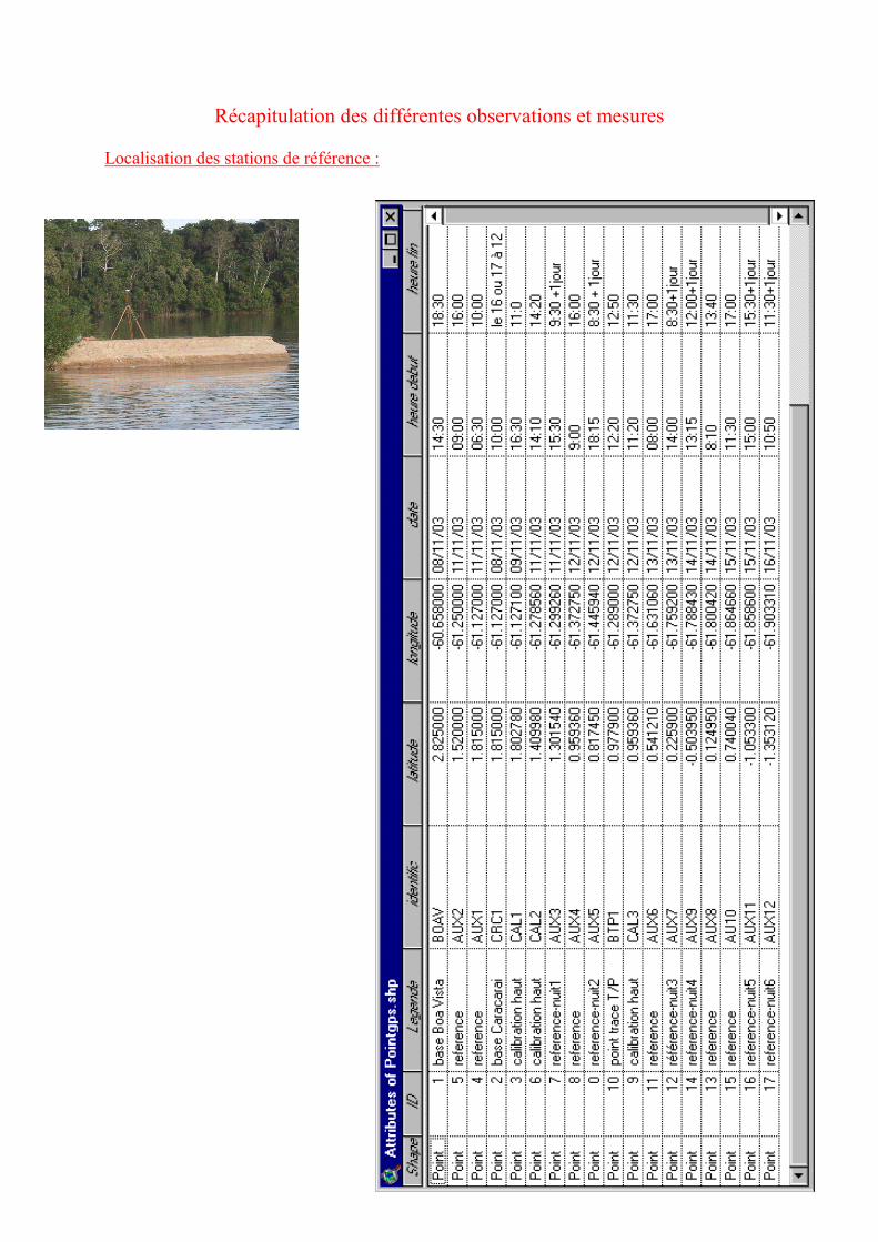
Récapitulation des différentes observations et mesures
Localisation des stations de référence :

Récapitulation des trajets GPS dynamiques :

Récapitulation des points bouées :

Récapitulation des trajets ADCP :

Nivellement des stations et points de mesure gravimétrique :
* Dans la table ci-dessous figurent seulement les bases gravimétriques. Des points de mesures
intermédiaires ont été réalisés tous les 10km environ (au niveau des jaugeages).

Points forme d’onde (autres que trajets GPS dyn):

Points d’observation géologique :

Hydrologie spatiale : Développement d’outils méthodologiques pour l’utilisation de la télédétection sur les
grands bassins fluviaux
Annexe 1 : Campagne de mesures de novembre 2003 sur le Rio Branco (Amazonie), Brésil
252

Hydrologie spatiale : Développement d’outils méthodologiques pour l’utilisation de la télédétection sur les
grands bassins fluviaux
Annexe 2 : Validation des hauteurs d’eau déduites des mesures altimétriques d’ENVISAT
253
Annexe 2 : Validation des hauteurs d’eau déduites des mesures
altimétriques d’ENVISAT
Résumé : Depuis le lancement du satellite ENVISAT en mars 2002, son altimètre radar
fournit des mesures de l’ensemble de la surface terrestre. Parmi les nombreux objectifs
d’ENVISAT, un est directement lié à l’hydrologie continentale: le suivi de l’évolution du
niveau d’eau des lacs, plaines d’inondation et fleuves. Les produits GDR d’ENVISAT
contiennent, sur tous les types de surface, quatre hauteurs altimétriques issues de différents
algorithmes de retraitement d’échos radar. Aucun d’entre eux n’ayant été développé pour le
traitement des formes d’onde altimétriques correspondant aux eaux continentales, il est
nécessaire d’évaluer leur performance pour le suivi des eaux continentales.
Dans ce but, quatre zones du bassin amazonien ont été sélectionnées pour effectuer une étude
de validation. Des comparaisons avec des stations limnimétriques ont montré que celui basé
sur le principe de l’estimation du centre de gravité de la forme d’onde [Wingham et al., 1986]
fournissait les meilleurs résultats.

Preliminary results of ENVISAT RA-2-derived water levels validation
over the Amazon basin
Frederic Frappart a,b,*, Stephane Calmant a, Mathilde Cauhope a,b,Frederique Seyler b, Anny Cazenave a
a Laboratoire d’Etudes en Geophysique et Oceanographie Spatiales, Observatoire Midi-Pyrenees, UMR 5566, CNES/CNRS/IRD/UPS,
18 Av. Edouard Belin, 31400 Toulouse, Franceb Laboratoire des Mecanismes de Transferts en Geologie, Observatoire Midi-Pyrenees, UMR 5563, CNRS/IRD/UPS, 18 Av. Edouard Belin, 31400 Toulouse, France
Received 11 April 2005; received in revised form 4 October 2005; accepted 8 October 2005
Abstract
Since the launch of the ENVISAT satellite in 2002, the Radar Altimetry Mission provides systematic observations of the Earth topography.
Among the different goals of the ENVISAT Mission, one directly concerns land hydrology: the monitoring of the water levels of lakes, wetlands,
and rivers. The ENVISAT Geophysical Data Records products contain, over different type of surfaces, altimeter ranges derived from four
specialized algorithms or retrackers. However, none of the retrackers are intended to the processing of the radar echoes over continental waters. A
validation study is necessary to assess the performances of the different ENVISAT-derived water levels to monitor inland waters. We have selected
four test-zones over the Amazon basin to achieve this validation study. We compare first the performances of these retracking algorithms to deliver
reliable water levels for land hydrology. Comparisons with in-situ gauge stations showed that Ice-1 algorithm, based on the Offset Centre of
Gravity technique, provides the more accurate water stages. Second, we examine the potentiality to combine water levels derived from different
sensors (Topex/Poseidon, ERS-1 and -2, GFO).
D 2005 Elsevier Inc. All rights reserved.
Keywords: Altimetry; Hydrology; Validation; Water levels
1. Introduction
The hydrological cycle of major river basins is strongly
influenced by both regional and global variations of the climate
system. As a consequence, monitoring the worldwide hydro-
logical cycle is of major importance for studies on the ongoing
climate changes. Many human activities such as transport,
water, and food resource management or land use are
dramatically dependent on our ability to monitor rivers and
associated floodplains water levels (Sippel et al., 1998).
Given the dramatic decrease in the number of in-situ gauges
observed in recent years (The Ad Hoc Group on Global Water
Datasets, 2001), the ability to measure river stages by satellite
has become a major goal in hydrology for the coming decades.
Koblinsky et al. (1993) were the first to process the Geosat
waveforms to estimate the water levels on four sites in the
Amazon basin. A RMS discrepancy between satellite and in-
situ measurements of 70 cm was estimated, mostly due to the
uncertainty in the orbit determination. The orbit determination
errors decreased with the new generations of satellite: the
uncertainty in radial component of satellite orbits is now
estimated to 3 cm for Topex/Poseidon (T/P) and 15 cm for
ERS-1 (Le Traon et al., 1995). Radar altimetry from T/P has
demonstrated the capability to monitor water level variations of
lakes, rivers, wetlands, and floodplains with a precision of
several tens of centimeters (Birkett, 1995, 1998; Maheu et al.,
2003; Mercier et al., 2002; Oliveira Campos et al., 2001).
The 12-year (1992–2004) hydrological dataset derived from
T/P measurements was expected to be extended with data from
Jason-1 and ENVISAT. Unfortunately, Jason-1 does not provide
land surface water measurements due to loss of surface lock by
the onboard tracker and inaccurate retracking procedure over
land surface water. Consequently, ENVISAT RA-2 is the only
0034-4257/$ - see front matter D 2005 Elsevier Inc. All rights reserved.
doi:10.1016/j.rse.2005.10.027
* Corresponding author. Laboratoire d’Etudes en Geophysique et Oceano-
graphie Spatiale, Centre National d’Etudes Spatiale, 18 Av. Edouard Belin,
31400 Toulouse, France.
E-mail addresses: [email protected] (F. Frappart),
[email protected] (F. Seyler).
Remote Sensing of Environment 100 (2006) 252 – 264
www.elsevier.com/locate/rse

operating altimeter (with Geosat Follow-On, a radar altimeter
launched in 1998 by the US Navy), able to monitor large rivers.
Similar to previous satellites with an on-board radar
altimeter, ENVISAT is able to provide altimeter measurements
of continental water heights (Gardini et al., 1995; Wehr &
Attema, 2001). In the present study, we use the first year of
ENVISAT RA-2 data to assess the performance of the mission
for continental water height measurements. Four range values
are provided conforming to four altimeter waveform retracking
algorithms.
The Amazon basin is the largest hydrographic basin in the
world, both in terms of area (¨6 million km2) and mean annual
discharge (¨200,000m3/s). It was the first large river basin to be
monitored with radar altimetry on its mainstream (Birkett, 1998;
Oliveira Campos et al., 2001). Using the dense network of gauge
stations of the Amazon basin, Birkett et al. (2002) achieved an
extensive validation study of water levels derived from Topex/
Poseidon radar altimeter over the 1992–1999 period. Compar-
isons with in-situ measurements reveal that the derived water
level time series have variable accuracy (mean¨1.1 mRMS and
best values ¨0.4–0.6 m RMS).
We present assessment of the water levels derived from
ENVISAT altimeter measurements over the Amazon basin. A
cross-comparison of the water levels derived from each
ENVISAT retracker is presented first, followed by comparisons
with in-situ measurements at different gauging sites and with
other altimeter datasets.
2. The ENVISAT Mission
In the framework of its Earth observation programme, the
European Space Agency (ESA) launched the ENVISATsatellite
on February 2002, a satellite designed to help the scientific
community to better understand the Earth environment and the
processes responsible for climatic changes. ENVISAT orbits on
a 35-day repeat cycle, providing observations of the Earth
surface (ocean and land) from 82.4- latitude North to 82.4-
latitude South, with an equatorial ground-track spacing of about
85 km. Two main objectives were identified for the ENVISAT
Mission (Gardini et al., 1995):
– collecting long time-series of the Earth’s environment at
global scale to observe trends,
– improving the capabilities to monitor and manage the
Earth’s resources and contributing to a better understanding
of the solid Earth processes.
To achieve these objectives, ENVISAT carries 10 scientific
instruments which provide atmosphere, ocean, land, and ice
measurements over the 5-year planned mission life-time (Wehr
& Attema, 2001). Its payload includes a radar altimeter
operating at two frequencies.
2.1. ENVISAT RA-2
The goal of RA-2 sensor is to provide a global scale
collection of radar echoes over ocean, land and ice to measure
ocean topography, water level variations over the large river
basins, land surface elevation, to monitor sea ice and polar ice
caps (Wehr & Attema, 2001). RA-2 is a nadir looking pulse
limited radar altimeter operating at two frequencies: 13.575
GHz (or 2.3 cm of wavelength) in Ku-band and 3.2 GHz (or
9.3 cm) in S-band (Zelli, 1999). Its beam footprint width is
about 3.4 km. The altimeter emits a radar pulse and measures
the two way travel-time from satellite to the surface (ocean,
ice, or land). The distance between the satellite and the Earth
surface–the altimeter height or range–is thus derived with a
precision of a few centimeters. A very precise orbit
determination is the result of the use of the DORIS system
(Doppler Orbitography and Radiolocation Integrated by
Satellite): an accuracy of around 6 cm is obtained for the
radial component of the satellite direction (Dow et al., 1999).
The altitude of the reflecting point with respect to a reference
ellipsoid is given by the difference between the satellite orbit
information and the range corrected for propagation delays.
Processing of radar echoes or altimeter waveforms is
performed on the ground to obtain accurate range values
(Zelli, 1999). In this study, we use the first available
ENVISAT RA-2 20 Hz range measurements contained in
the Geophysical Data Records (GDRs) (ESA, 2002) from
cycle 14 to cycle 25 of ENVISAT RA-2 Mission (February
17, 2003 to March 12, 2004).
2.2. Retracking procedures
Radar altimetry has many limitations over land due to the
complexity of returned waveforms. An altimeter waveform
(or radar echo) represents the histogram of the energy
backscattered by the ground surface to the satellite with
respect to time. Many radar echoes are multipeaked or
present a noisy shape revealing the presence in the altimeter
footprint of several reflectors such as water, vegetation
canopy, rough topography or vegetation (see Wingham et
al., 1986 for a classification of the radar echoes over
continental surfaces).
Accurate range estimates are obtained using refined
procedures known as altimeter waveform retracking. Altimeter
waveform retracking consists in ground-processing altimeter
waveforms to obtain better range estimates than those obtained
with on-board tracking algorithms. The algorithm retrieves the
point of the radar echo corresponding to the effective satellite-
to-ground range.
For the ENVISAT mission, four different retrackers are
operationally applied to RA-2 raw-data to provide accurate
height estimates. Each retracker has been developed for a
specific surface response: one for ocean, two for ice sheets, and
one for sea ice. It is worthy to notice that none of them was
developed for processing altimeter waveforms over continental
waters. Thus, none among these algorithms is supposed to
retrieve reliable range values for land water studies.
2.2.1. Ocean and Ice-2 retrackers
Two of the retracking schemes, referred as Ocean and Ice-2
and applied to the RA-2 measurements, are based on the Brown
F. Frappart et al. / Remote Sensing of Environment 100 (2006) 252–264 253

(1977) model. According to this theoretical model, the
waveform (Eq. (1)) can be described as the double convolution
of the radar pulse, the radar point target response, and the
probability density of the specular points on the surface
(Rodriguez & Chapman, 1989):
Pr tð Þ ¼ Pe tð ÞTfptr tð Þ4gpdf zð Þ ð1Þ
where Pr(t): return power, Pe(t): emitted power, fptr(t): radar
point target function (including the antenna gain of the sensor),
and gpdf(z): probability density function of the specular points on
the surface.
For the Ocean tracker, the classical waveform shape (Fig. 1a)
proposed by Brown (1977) is used. The ocean retracking algorithm
objective is to fit themeasuredwaveformwith a return powermodel
(ESA, 2002), according to weighted least square estimators using
the Levenberg-Marquardt’s method (Press et al., 1992). The
expression of the model versus time is derived from Hayne’s
(1980) model.
Fig. 1. Retracking schemes: (a) Ocean (from CNES), (b) Ice-1 (from Bamber, 1994), (c) Ice-2 (from Legresy & Remy, 1997), (d) Sea Ice (from ESA, 2002).
Fig. 2. Location of the study zones: Tabatinga area (1), Negro River sub-basin (2), Solimoes-Negro confluence (3), and Tapajos River (4).
F. Frappart et al. / Remote Sensing of Environment 100 (2006) 252–264254

The Ice-2 retracker, intended for ice caps studies, consists in
detecting the waveform edge (Fig. 1b), fitting an error function
(erf) to the leading edge and an exponential decrease to the
trailing edge (Legresy & Remy, 1997). It is assumed that the
trailing effects do not dramatically affect the leading edge part
of the waveform. As a consequence, the two parts of the
waveform can be fitted separately (Legresy, 1995).
2.2.2. Ice-1 retracker
Ice-1 retracker is intended to estimate heights of ice caps and
more generally land surfaces. This algorithm is based on the
Offset Centre of Gravity (OCOG) method developed by
Wingham et al. (1986) and applied by Bamber (1994) to the
ERS-1 and -2 data. This retracking method is a threshold
approach, which requires the estimate of the waveform
amplitude. The crucial point in this technique lies in the estimate
of the waveform amplitude, which must be insensitive to speckle
noise and variations in waveform shape (Bamber, 1994). The
effects of noise are reduced as the number of samples increases.
The algorithm calculates the centre of gravity, amplitude, and
width of a rectangular box using the maximum of the waveform
samples (Fig. 1c). The amplitude of the box is twice the value of
the centre of gravity. In Eqs. (2)–(4), the square of the sample
values are used to reduce the effect of low amplitude samples in
front of and in the leading edge (Wingham et al., 1986).
centre of gravity ¼
X
n¼Naln
n¼1þaln
ny2 nð Þ
X
n¼Naln
n¼1þaln
y2 nð Þ
ð2Þ
amplitude ¼
ffiffiffiffiffiffiffiffiffiffiffiffiffiffiffiffiffiffiffiffiffiffiffiffiffiffi
X
n¼Naln
n¼1þaln
y4 nð Þ
X
n¼Naln
n¼1þaln
y2 nð Þ
v
u
u
u
u
u
u
u
t
ð3Þ
width ¼
X
n¼Naln
n¼1þaln
y2 nð Þ
! 2
X
n¼Naln
n¼1þaln
y4 nð Þ
ð4Þ
where y is the value of the nth sample and aln is the number of
aliased bins at the beginning and end of the waveform.
The nominal tracking position (Fig. 1c) is determined by
finding the point on the waveform (by interpolation) where the
amplitude exceeds a threshold (25% of the amplitude).
2.2.3. Sea ice retracker
As no model currently describes sea ice waveforms, no
multi-parameter fit of the radar echo can be retrieved. A
straightforward threshold technique was developed to retrack
data over sea ice (Laxon, 1994). The sea-ice waveform
amplitude is first identified by finding the maximum value of
the echo (Eq. (5)):
amplitude ¼ maxnaN y nð Þð Þ ð5Þ
where y is the value of the nth sample of the waveform and N is
the number of waveform samples.
The tracking offset (Fig. 1d) is determined by finding the
point on the waveform, using linear interpolation, where the
radar echo is greater than a threshold corresponding to half
the waveform amplitude (ESA, 2002; Laxon, 1994).
3. Altimetry validation datasets
3.1. Topex/Poseidon radar altimetry data
The measurements used in this study are the 10 Hz Ku-
range estimates contained in the GDRs delivered by the
Table 2
Location and altitude of the in-situ gauge stations
Station Basin Longitude
(-)
Latitude
(-)
Stage-0 altitude
(m wrt GRACE)
Tabatinga Solimoes-Amazon 69.933 4.25 55.98
Manacapuru Solimoes-Amazon 60.609 3.308 3.87
Obidos Solimoes-Amazon 55.511 1.947 2.41
Curuai Solimoes-Amazon 55.476 2.267 0.77
Tabatinga do Sale Solimoes-Amazon 55.78 2.25 4.55
Curicuriari Negro 66.812 0.192 32.46
Tapuracuara Negro 65.015 0.42 25.45
Manaus Negro 60.035 3.149 7.5
Table 1
Geographical extension of the study zones
Zone Longitude (-) Latitude (-)
Min Max Min Max
Tabatinga 70.69 69.59 4.85 3.67
Negro River sub-basin 73.25 59.35 3.35 5.4
Solimoes-Negro conf. 62.47 58.01 4.22 1.05
Tapajos 56.1 54.43 3.82 1.54Fig. 3. Location of ENVISAT tracks on lower Tapajos.
F. Frappart et al. / Remote Sensing of Environment 100 (2006) 252–264 255
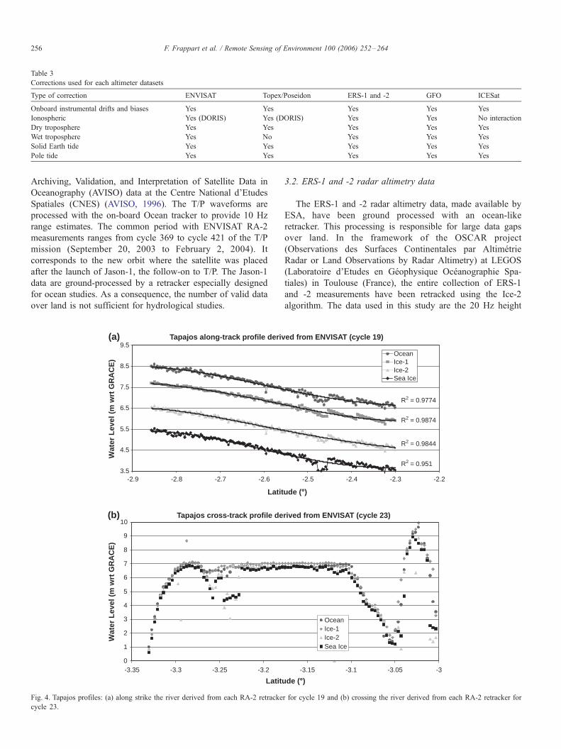
Archiving, Validation, and Interpretation of Satellite Data in
Oceanography (AVISO) data at the Centre National d’Etudes
Spatiales (CNES) (AVISO, 1996). The T/P waveforms are
processed with the on-board Ocean tracker to provide 10 Hz
range estimates. The common period with ENVISAT RA-2
measurements ranges from cycle 369 to cycle 421 of the T/P
mission (September 20, 2003 to February 2, 2004). It
corresponds to the new orbit where the satellite was placed
after the launch of Jason-1, the follow-on to T/P. The Jason-1
data are ground-processed by a retracker especially designed
for ocean studies. As a consequence, the number of valid data
over land is not sufficient for hydrological studies.
3.2. ERS-1 and -2 radar altimetry data
The ERS-1 and -2 radar altimetry data, made available by
ESA, have been ground processed with an ocean-like
retracker. This processing is responsible for large data gaps
over land. In the framework of the OSCAR project
(Observations des Surfaces Continentales par Altimetrie
Radar or Land Observations by Radar Altimetry) at LEGOS
(Laboratoire d’Etudes en Geophysique Oceanographie Spa-
tiales) in Toulouse (France), the entire collection of ERS-1
and -2 measurements have been retracked using the Ice-2
algorithm. The data used in this study are the 20 Hz height
Table 3
Corrections used for each altimeter datasets
Type of correction ENVISAT Topex/Poseidon ERS-1 and -2 GFO ICESat
Onboard instrumental drifts and biases Yes Yes Yes Yes Yes
Ionospheric Yes (DORIS) Yes (DORIS) Yes Yes No interaction
Dry troposphere Yes Yes Yes Yes Yes
Wet troposphere Yes No Yes Yes Yes
Solid Earth tide Yes Yes Yes Yes Yes
Pole tide Yes Yes Yes Yes Yes
(a)
(b) Tapajos cross-track profile derived from ENVISAT (cycle 23)
0
1
2
3
4
5
6
7
8
9
10
-3.35 -3.3 -3.25 -3.2 -3.15 -3.1 -3.05 -3
Wat
er L
evel
(m
wrt
GR
AC
E)
OceanIce-1Ice-2Sea Ice
Tapajos along-track profile derived from ENVISAT (cycle 19)
R2 = 0.9774
R2 = 0.9874
R2 = 0.9844
R2 = 0.9513.5
4.5
5.5
6.5
7.5
8.5
9.5
-2.9 -2.8 -2.7 -2.6 -2.5 -2.4 -2.3 -2.2
Latitude ( °)
Latitude ( °)
Wat
er L
evel
(m
wrt
GR
AC
E)
OceanIce-1Ice-2Sea Ice
Fig. 4. Tapajos profiles: (a) along strike the river derived from each RA-2 retracker for cycle 19 and (b) crossing the river derived from each RA-2 retracker for
cycle 23.
F. Frappart et al. / Remote Sensing of Environment 100 (2006) 252–264256

derived from ERS-1 and -2 range estimates retracked with
Ice-2 algorithm for 1991–2003.
3.3. Geosat Follow-On radar altimetry data
Geosat Follow-On (GFO) is a US Navy altimeter mission
launched in 1998. The data have been delivered to the scientific
community since November 9, 2000. An Ocean-like tracking
algorithm is applied to the GFO waveforms to derive range
measurements. We used the 10 Hz height estimates made
available by the National Oceanic and Atmospheric Adminis-
tration (NOAA) from cycle 55 to 124 (November 9, 2000 to
February 16, 2004).
3.4. ICESat radar altimetry data
The Ice, Cloud, and Land Elevation Satellite (ICESat) is part
of NASA’s Earth Observation System (EOS) to measure
changes in elevation of the Earth surface and primarily the
Greenland and Antarctic Ice sheets. ICESat is supposed to
provide independent high-accuracy data to calibrate and
validate topographic products (Zwally et al., 2002). In this
study, we use the Release 19 of the GLAS/ICESat L2 Global
Land Surface Altimetry Data product (Zwally et al., 2000)
made available by the National Snow and Ice Data Center
(NSIDC—http://nsidc.org/daac/icesat).
4. The study regions
Our study is focused on four regions of the Amazon basin
(Fig. 2): the area surrounding Tabatinga, the Negro River sub-
(a) (b)
(c) (d)
8
10
12
14
16
18
20
22
11/5/2001 5/24/2002 12/10/2002 6/28/2003 1/14/2004 8/1/2004 11/5/2001 5/24/2002 12/10/2002 6/28/2003 1/14/2004 8/1/2004
11/5/2001 5/24/2002 12/10/2002 6/28/2003 1/14/2004 8/1/200411/5/2001 5/24/2002 12/10/2002 6/28/2003 1/14/2004 8/1/2004
Date
Date Date
Date
Wat
er L
evel
(m
wrt
GR
AC
E)
Wat
er L
evel
(m
wrt
GR
AC
E)
Wat
er L
evel
(m
wrt
GR
AC
E)
Wat
er L
evel
(m
wrt
GR
AC
E)
GaugeOcean
8
10
12
14
16
18
20
22
8
10
12
14
16
18
20
22
8
10
12
14
16
18
20
22
GaugeSea Ice
GaugeIce-1
Gauge
Ice-2
Fig. 5. Time series of water level derived from each ENVISAT retracker 29 km upper Manaus and compared with Manaus gauge measurements. The grey lines
represent in-situ water level measurements; dark dots stand for water levels derived from Ocean (a), Ice-1 (b), Ice-2 (c), and Sea Ice (d) retrackers. Black lines are the
uncertainties on ENVISAT measurements.
Table 4
RMSE between water levels derived from ENVISAT for each retracker and
water levels measured at in-situ stations
Reference ENVISAT track RMS error (m)
Station Position (km) Ocean Ice-1 Ice-2 Sea Ice
Tabatinga 20 lower 0.27 0.40 0.32 1.37
Manacapuru 43.5 upper 0.27 0.20 0.86 0.69
Manacapuru 43.5 lower 0.31 0.27 0.29 0.21
Obidos 5.25 lower 0.26 0.26 0.58 0.4
Curuai Lake 1 0.85 0.36 0.90 1.08
Curuai Lake 2 1.40 0.25 1.10 3.24
Curuai Lake 3 0.55 0.53 1.35 0.99
Curicuriari 29 upper 0.12 0.07 0.10 0.13
Tapuruquara 15.5 upper 0.50 0.35 0.42 0.33
Tapuruquara 47.5 lower 0.42 0.12 0.23 0.14
Manaus 29 upper 0.31 0.11 0.56 0.32
F. Frappart et al. / Remote Sensing of Environment 100 (2006) 252–264 257

basin, the confluence between Negro and Solimoes Rivers, and
the lower part of the Tapajos River with the varzea of Curuai.
The locations are summarized in Table 1. These areas are
monitored by the HYBAM project (Hydrologie du Bassin
Amazonien or Hydrology of the Amazon Basin) for their
hydrological interest. The Brazilian Water Agency (Agencia
Nacional de Aguas or ANA) is in charge of managing a network
of 571 gauging stations in the Brazilian part of the Amazon basin
(http://www.ana.gov.br). At each station, daily measurements of
water stage are collected and daily estimates of discharge are
produced using rating curves, obtained from periodic (some-
times several times a year) simultaneous measurements of stage
and discharge. Some of these stations are GPS levelled. To
validate the RA-2-derived water levels, we selected eight in-situ
gauge stations from this database that comply with the following
criteria: the station is levelled and water stage data are available
between 2003 and the beginning of 2004, the station is in the
vicinity (less than 50 km) of an ENVISAT ground-tracks. The
location of the eight stations selected for this study is presented
in Table 2. Many gauge stations were discarded because they
were not levelled. This strict selection criteria were applied to
perform a validation study on absolute water stages rather than
on relative level changes.
5. Inter comparison of the retrackers
In this part, profiles of the Tapajos River estimated by the
four retrackers are compared. Two typical cases are presented
(Fig. 3): the satellite track runs along strike the river (track 764)
and the satellite track crosses the river (track 349). Water levels
are obtained as the difference between the values of the satellite
orbit and the range values, taking into account different
instrumental and geophysical corrections to the range. The
corrections applied to the different sensors, contained in the
ENVISAT, ERS-1 and -2, T/P, GFO GDRs, and in ICESat/
GLAS standard data products are listed in Table 3. On the
lower Tapajos, track 764 acquires water level along 80 km long
profiles. To quantify the dispersion, fourth order polynoms are
fitted on these profiles each cycle. On Fig. 4a, profiles derived
from Ice-1, Ice-2, and Sea Ice for cycle 19 are artificially
shifted downward by respectively 1, 2, and 3 m of their actual
level. In average for all the cycles, the number of valid points is
greater than 95% of the available measurements, the root mean
square (RMS) discrepancies between measurements and poly-
noms are 0.1, 0.09, 0.11, and 0.13 m, and the correlation
coefficient are 0.98, 0.98, 0.97, and 0.95, respectively, for
Ocean, Ice-1, Ice-2, and Sea Ice. All these profiles exhibit a
10
9
8
7
6
5
4
3
2
10
9
8
7
6
5
4
3
2
10
9
8
7
6
5
4
3
2
10
9
8
7
6
5
4
3
205/11/01 24/05/02 10/12/02 28/06/03 14/01/04 01/08/04 05/11/01 24/05/02 10/12/02 28/06/03 14/01/04 01/08/04
05/11/01 24/05/02 10/12/02 28/06/03 14/01/04 01/08/0405/11/01 24/05/02 10/12/02 28/06/03 14/01/04 01/08/04
Wat
er L
evel
(m
wrt
GR
AC
E)
Wat
er L
evel
(m
wrt
GR
AC
E)
Wat
er L
evel
(m
wrt
GR
AC
E)
Wat
er L
evel
(m
wrt
GR
AC
E)
Date Date
Date Date
(a) (b)
(c) (d)
GaugeOcean
GaugeIce-2
GaugeIce-1
GaugeSea lce
Fig. 6. Time series of water level derived from each ENVISAT retracker at Curuai lake 2 and compared with Curuai gauge measurements. The grey lines represent in-
situ water level measurements; dark dots stand for respectively water levels derived from Ocean (a), Ice-1 (b), Ice-2 (c), and Sea Ice (d) retrackers. Black lines are the
uncertainties on ENVISAT measurements.
F. Frappart et al. / Remote Sensing of Environment 100 (2006) 252–264258

similar curvature for all the dates. The water levels are
consistent with hydrological observations in this part of the
basin: maxima are recorded between June and August whereas
minima are observed between mid-October and January.
In most cases, the satellite ground track only intersects the
river over a few kilometers and the width of the river changes
from a cycle to another with the water level. The intersection
of track 349 with Tapajos River is located between latitude
3.1-S and 3.27-S. Each of the four retrackers provides
realistic estimate of the water level (Fig. 4b). Nevertheless,
some height measurements derived from Ocean, Ice-2, and
Sea Ice are clearly erroneous with underestimation of water
levels up to several meters for latitude greater than 3.2-S.
Similar situations are observed in different comparable
configurations on the Amazon basin, where water levels
derived from Ice-1 are more reliable than the estimations
provided by the other retrackers.
6. Comparison with in-situ gauge stations
For each intersection between the river and the satellite
ground-track, we define a so-called ‘‘virtual station’’, that
represents a rectangular window. Each cycle, the water level
at a given virtual station is obtained by computing the median
of all the high-rate data (20 Hz for ENVISAT RA-2, ERS-1
and -2, and 10 Hz for T/P and GFO) included in the
rectangular window. This process, repeated each cycle, allows
the construction of the time series of water level associated
with a virtual station. The corrections applied to the different
sensors, contained in the ENVISAT, ERS-1 and -2, T/P, GFO
GDRs, and in ICESAT/GLAS standard data products are
listed in Table 3.
The dispersion in L1 norm is given by the estimator known
as median absolute deviation (Eq. (6)):
MAD xð Þ ¼1
N 1
X
N
i¼1
jxi xmedj ð6Þ
where MAD(x): median absolute deviation of the observations,
N: number of observations, xi: ith observation, and xmed:
median of the observations.
Water levels are referenced to geoid EIGEN-GRACE02S,
complete to order 150 (Reigber et al., 2005). This geoid is
derived from the first year of the GRACE satellite gravimetry
mission measurements which monitored the time–space
variations of the gravity field with a resolution of 2-2- at
the equator and an accuracy of 1 cm on the geoid height
(Reigber et al., 2005).
The water level time series derived from the four
retrackers are compared with in-situ gauge stations measure-
ments. 8% to 15% more valid data are found when retracked
with Ice-1 compared with other retrackers. The dispersion (in
L1-norm) is lower with Ice-1 than other retrackers, typically
lower than 0.2 and 0.1 m for low and high stage,
Fig. 7. Location of the ENVISAT tracks on the varzea of Curuai and of the in-
situ gauge station.
10
9
8
7
6
5
4
3
205/11/01 24/05/02 10/12/02 28/06/03 14/01/04 01/08/04
GaugeIce-1
Wat
er L
evel
(m
wrt
GR
AC
E)
Date
(b)
10
9
8
7
6
5
4
3
205/11/01 24/05/02 10/12/02 28/06/03 14/01/04 01/08/04
GaugeIce-1
Wat
er L
evel
(m
wrt
GR
AC
E)
Date
(a)
10
9
8
7
6
5
4
3
2
05/11/01 24/05/02 10/12/02 28/06/03 14/01/04 01/08/04
Ice-1
Wat
er L
evel
(m
wrt
GR
AC
E)
Date
(c)
Gauge
Fig. 8. Time series of water level derived from ENVISAT RA-2 measure-
ments retracked with Ice-1 at Curuai lake 1 (a), Curuai lake 2 (b), Curuai lake
3 (c), and compared with in-situ gauge measurements. The grey lines
represent in-situ water level measurements; dark dots stand for water levels
derived from Ice-1 retracker. Black lines are the uncertainties on ENVISAT
measurements.
F. Frappart et al. / Remote Sensing of Environment 100 (2006) 252–264 259

respectively. Dispersion can decrease to 0.05 m when the
river is large enough as in Manaus (Fig. 5). RMS errors
between altimeter-derived and in-situ water levels are
presented in Table 4. In all cases, Ice-1 exhibits the lowest
RMS errors compared to the other retrackers. Better results
are obtained on rivers than on wetlands (the example of the
three lakes of Curuai varzea, see Lake 2 on Fig. 6). The Ice-1
retracker appears to be the best suited for hydrological
applications and we decided to use the Ice-1 retracked data in
the following sections.
7. Validation over the varzea of Curuai
The varzea of Curuai, located south of Obidos city, can
be considered as representative of a large number of
inundation systems disseminated along the Amazon flood-
plain. It is composed of twenty or so interconnected lakes
linked to the river by temporary and permanent channels, of
more than one hundred kilometres long on the south
riverside (Fig. 7). Its hydrological functioning is monitored
by the HYBAM project, which has collected in-situ
measurements during 17 scientific campaigns. One of the
main interrogation concerns the relevance of altimetry from
space data for hydrological purposes, i.e. the understanding
of the functioning of the floodplain in terms of nature of
data, accuracy, and coherency with in-situ measurements.
On the varzea of Curuai, three different lakes where water
levels time series can be constructed were identified. The time
Table 5
Comparison of water levels from in-situ gauge stations and derived from RA-2 over the varzea of Curuai
r (m) Bias (m) RMSE (m) Correlation coefficient Linear regression: y =ax +b ra rb (m)
Lake 1 0.22 0.71 0.36 0.98 y =0.94x+1.1 0.24 0.08
Lake 2 0.30 0.24 0.25 0.99 y =0.89x+0.5 0.19 0.06
Lake 3 0.58 0.32 0.53 0.96 y =1.01x0.43 0.52 0.17
10.5
9.5
8.5
7.5
6.5
5.5
4.53.5 4.5 5.5 6.5 7.5 8.5 9.5
Wat
er le
vel d
eriv
ed fr
om R
A-2
(m
)
Water level at Tabatinga do salé station (m)
y = 0.94x + 1.10
(a)
4 5 6 7 8 9 10
10
9
8
7
6
5
4
33
Water level at Curuai station (m)
Wat
er le
vel d
eriv
ed fr
om R
A-2
(m
)
y = 1.01x - 0.43
(c)
10
9
8
7
6
5
4
4 5 6 7 8 9 103
Water level at Tabatinga do salé station (m)
Wat
er le
vel d
eriv
ed fr
om R
A-2
(m
)
y = 0.89x + 0.50
(b)
Fig. 9. Water levels at Curuai in-situ gauge station versus water levels derived
from RA-2 (Ice-1 retracker) for lake 1 (a), lake 2 (b), and lake 3 (c). Fig. 10. Altimeter tracks on lower Tapajos.
F. Frappart et al. / Remote Sensing of Environment 100 (2006) 252–264260

series obtained with Ice-1 are then compared with the in-situ
station of Tabatinga do Sale for lakes 1 and 2 and Curuai for
lake 3 (Fig. 8). To discuss the accuracy of the results, five
estimators have been taken into consideration:
– the dispersion of high-rate data estimated with (Eq. (6)) and
averaged for all the cycles,
– the mean bias between RA-2 and in-situ measurements,
– the RMSE between RA-2 and in-situ measurements,
– the correlation coefficient between RA-2 and in-situ
measurements,
– the equation of the linear regression.
Their values are computed for the three lakes with the
results of Ice-1 retracking algorithm and listed in Table 5. The
corresponding scatter plots are presented on Fig. 9.
The dispersion on the derived water levels is low (<0.3 m)
except for lake 3 (0.58 m). The high value obtained on lake 3
can be explained by the nature of the intersection between the
satellite ground track and the lake: its width is only several
hundred meters between sandbars covered with vegetation. As
a consequence, the quality of altimeter measurement is affected
by the complex environment (reflections from water, ground,
and canopy vegetation) encompassed in the altimeter footprint.
The biases between RA-2 and in-situ measurements range from
0.32 and 0.7 m. The in-situ gauge stations of Tabatinga do
Sale and Curuai were levelled by GPS. A priori, such biases
can hardly be attributed to errors in the levelling of the stations.
It is worth noting that the gauges are several tens of kilometres
away from the varzea lakes. So, short wavelength geoid
undulations, not described in the EIGEN-GRACE02C geoid,
may produce level biases between gauges and lakes. Errors in
the geophysical corrections applied to the RA-2 ranges may be
also responsible for these differences. Yet, these biases are most
likely caused by lack of accuracy on range estimation or have
hydrological causes. The level of the different lakes composing
Fig. 11. Multi-satellite water level time series at 3.2-S (a) and 2.6-S (b).
Table 6
Biases and RMS discrepancies between water levels derived from altimeter
datasets and pseudo in-situ time series on the lower Tapajos: (a) at 3.2-S (box
A) and (b) at 2.6-S (box B)
Bias (m) RMS (m)
(a)
ERS 349 0.0* 0.68
ERS 764 0.0* 0.43
ENV. 349 0.22 0.14
ENV. 764 0.65 0.43
GFO 63 0.07 0.54
(b)
ERS 764 0.0* 0.2
ENV. 764 0.76 0.2
T/P 50 0.39 0.35
F. Frappart et al. / Remote Sensing of Environment 100 (2006) 252–264 261

the varzea is not necessary the same and is not constant on their
whole surface (slopes of 2 cm/km were recorded using ICESat
measurements). Clearly, further study is necessary to determine
the actual causes of these differences. Nevertheless, correlation
coefficients between water levels derived from RA-2 measure-
ments and in-situ records are all greater than 0.95: the water
level variations are hence well estimated. This analysis
demonstrates the great quality of the ENVISAT measurements
retracked with Ice-1.
8. Multi-satellite validation
The time sampling (respectively 10, 15, and 35 days for T/P,
GFO, and ERS-1 and -2/ENVISAT) of the present radar
altimetry missions is not sufficient to monitor rapid changes in
hydrological processes. The combination of water levels derived
from the different satellites increases the time sampling at cross-
over points. Two zones were identified on the lower Tapajos
where ENVISAT tracks are crossing other altimeter tracks (Fig.
10). ENVISAT track 349 intersects T/P track 50 at 2.6- S (box
A). ENVISAT tracks 764 and 349 form a cross-over point and
both intersect GFO track 063 at 3.2- S (box B). The combined
water level time series are presented on Fig. 11a and b. There is
no in-situ gauge station on the lower Tapajos to record water
stages. In order to compare the different altimetry datasets to a
common reference, we have created a pseudo time series from
remote stations. Measurements from the two closest stations–
Itaituba on the upstream part of the Tapajos and Obidos on the
Amazon River–have been used. Best agreement has been found
with Obidos station, scaling the stage variations by 0.87. This
scale factor accounts for the difference in width between lower
Tapajos and the Amazon River in Obidos. These pseudo in-situ
time series have been further levelled at the location of boxes A
and B using ICESat measurements. Biases and RMS discre-
pancies for all the time series are reported in Table 6. The biases
for the ERS series are zero by construction since these data
undergo a long wavelength—geographical-error and the time
series have been best-fit adjusted to the in-situ series. Biases and
RMS scatter for the ENVISAT series are similar to those
obtained for the other missions. GFO presents the smallest bias
(0.07 m) but ENVISAT series present the lowest RMS scatter
(0.2 m). In addition, the RMS discrepancies obtained with
datasets on-board tracked using ‘‘ocean-like’’ trackers (T/P and
GFO) are larger than those obtained with the Ice-2 (ERS series)
and Ice-1 (ENVISAT series) retrackers. These preliminary
results are very promising. Nevertheless, as the measurement
dates do not coincide, the datasets can not be fully cross-
calibrated to determine the biases between each satellite as it is
done for oceanography (Le Traon et al., 1995). When longer
time-series of ENVISAT water levels are available, minimiza-
tion of cross-over differences will be performed to determine the
relative biases between the missions and enable to produce time
series combining all the altimeter data available at every virtual
station.
9. Migration of RA-2 altimeter data
Lakes, rivers, and wetlands water level profiles derived from
altimeter measurements are expected to be flat or slightly
inclined. Downward turning parabolic features that are clearly
artefacts are commonly observed on altimeter profiles over the
water bodies (see example in Fig. 12). This problem occurs
when the altimeter tracker is locked on the brighter target
present in the footprint and does not estimate the actual slant
distance between the satellite and the target in the nadir
direction. The round-trip travel time between the altimeter and
the at-nadir surface (and the range as a consequence) is thus
over estimated. As shown on Fig. 13, the error in the height
estimate can be approximated by (Eq. (7)):
Dh ¼ hV h ¼ h
ffiffiffiffiffiffiffiffiffiffiffiffiffiffiffiffiffiffiffiffiffiffi
1þd
h
2s
1
0
@
1
A,
d2
2h; dbh ð7Þ
where Dh is the height error, h the actual range of the water
body, hV the measured range, and d the along-track distance
between the satellite nadir and the target.
The migration method consists of integrating energy over
such parabolic features and focusing the resultant sum at the
apex of the curve. It was already used in altimetry over ice caps
to improve the resolution of topographic features (Nuth et al.,
2002). We do not apply the migration technique to the altimeter
waveform data but to the Ice-1 ranges over lake 2 of Curuai
varzea. For each cycle, we have compared the water levels to
those obtained after migration. We can thus estimate the error
without migrating altimeter data. For the whole time series, the
RMS discrepancy between water levels at Curuai gauge station
Curuai Varzea profile derived from ENVISAT (Cycle 14)8.58.38.17.97.77.57.37.16.96.76.5
-2.3 -2.25 -2.2 -2.15 -2.1 -2.05 -2 -1.95 -1.9
Latitude ( °°)
Wat
er L
evel
(m
wrt
GR
AC
E)
Lake 3
Lake 2
Ice-1Ice-1 migrated
Fig. 12. Water level profile derived from ENVISAT 20-Hz measurements over
Curuai Varzea.
hh'
d
Fig. 13. Principle of migration.
F. Frappart et al. / Remote Sensing of Environment 100 (2006) 252–264262

and those derived from RA-2 is 0.27 m. After the migration
process, the RMSE is reduced to 0.19 m. This simple example
illustrates the importance of radar altimetry data migration for
hydrological studies.
10. Conclusion
ENVISAT RA-2 exhibits a strong capability for the
monitoring of inland waters. Among the four retracking
algorithms applied to ENVISAT waveforms, Ice-1 provides
the most suited ranges for continental hydrology studies. For
the different test zones, the large number of valid data with the
lowest RMS differences (<0.3 m on the rivers and <0.5 m on
the wetlands) are obtained for water levels derived from Ice-1
retracker. These results, for 1 year of RA-2 data, are two or
three times better than those obtained with 10-year of T/P data
by Birkett et al. (2002). A particularly accurate monitoring of
water stages with ENVISAT RA-2 is, hence, expected. The
dispersion on the measurement does not exceed 0.2 m and
most of the time is lower than 0.15 m. Nevertheless, an
important number of data are lacking in the ENVISAT RA-2
GDRs: for a given virtual station, there is no available data for
various cycles. To improve the accuracy of the altimeter-
derived hydrological datasets, it is necessary to perform
migration process. These preliminary results have to be
confirmed for large river basins in different regions (tropical,
mid-latitude, and polar regions). Nevertheless, these results
demonstrate the interest to retrack the waveforms from the
present radar altimeter missions (T/P, ERS-1 and -2, Jason-1,
GFO) to increase the number of available data and improve the
accuracy for continental water studies.
Furthermore, to assess the accuracy of RA-2 for land water
studies, absolute range calibration should be performed using
the same type of experiments as for ocean (Roca et al., 2003).
Cross-calibration of the present radar altimeters is necessary to
combine the datasets for hydrological purposes.
Different hydrological applications of RA-2-derived water
levels can be foreseen. As RA-2 efficiently completes the
present network of altimeter gauge stations on rivers and
wetlands, a better understanding of the hydrological processes
at basin scale is forthcoming. Moreover, the estimation of the
time variations of water volume during floods can be envisaged
by combining water levels derived from RA-2 raw-data and
simultaneously acquired MERIS or ASAR images for the
delineation of the inundated areas. Finally, the assimilation of
RA-2 data in hydrological models can improve the quality of
their outputs and predictions and become the first step toward
operational hydrology.
Acknowledgements
This paper is a contribution to the validation of ESA
ENVISAT RA-2. The authors wish to thank Benoıt Legresy
from Laboratoire des Etudes en Geophysique et Oceanographie
Spatiales (LEGOS, Toulouse, France) for the delivery of ERS-
1 and -2 data retracked with Ice-2 algorithm and for fruitful
discussions. ENVISAT RA-2, T/P and GFO data were
provided by the Centre de Topography des Oceans et de
l’Hydrosphere (CTOH) at LEGOS. One of the authors (FF) is
supported by a CNES/Alcatel Space grant. We are particularly
grateful to Nelly Mognard-Campbell, from LEGOS, for
reviewing the English version of the paper.
References
Ad Hoc Work Group on Global Water Datasets. (2001). Global water data: An
endangered species. EOS Transactions American Geophysical Union, 82,
54–58.
AVISO. (1996). AVISO user handbook: Merged TOPEX/POSEIDON products,
AVI-NT-02-101-CN (3-rd edR). Toulouse, France’ CNES, 194 pp.
Bamber, J. L. (1994). Ice sheet altimeter processing scheme. International
Journal of Remote Sensing, 15(4), 925–938.
Birkett, C. M. (1995). The contribution of TOPEX/POSEIDON to the global
monitoring of climatically sensitive lakes. Journal of Geophysical Re-
search, 100(C12), 25,179–25,204.
Birkett, C. M. (1998). Contribution of the TOPEX NASA radar altimeter to the
global monitoring of large rivers and wetlands. Water Resources Research,
34(5), 1223–1239.
Birkett, C. M., Mertes, L. A. K., Dunne, T., Costa, M. H., & Jasinski, M. J.
(2002). Surface water dynamics in the Amazon basin: Application of
satellite radar altimetry. Journal of Geophysical Research, 107(D20),
8059–8080.
Brown, G. S. (1977). The average impulse response of a rough surface and
is applications. IEEE Transactions on Antennas and Propagation, 25(1),
67–74.
Dow, J. M., Martinez Fadrique, F. M., & Zandbergen, R. (1999). High precision
altimetry from the ENVISAT mission. Advances in Space Research, 23(4),
757–762.
ESA. (2002). ENVISAT RA2/MWR Product Handbook, RA2/MWR Products
User Guide.
Gardini, B., Graf, G., & Ratier, G. (1995). The instruments on ENVISAT. Acta
Astronautica, 37, 301–311.
Hayne, G. S. (1980). Radar altimeter mean return waveforms from near-
normal-incidence ocean surface scattering. IEEE Transactions on Antennas
and Propagation, 28(5), 687–692.
Koblinsky, C. J., Clarke, R. T., Brenner, A. C., & Frey, H. (1993).
Measurements of river level variations with satellite altimetry. Water
Resources Research, 29(6), 1839–1848.
Laxon, S. (1994). Sea ice altimeter processing scheme at the EODC.
International Journal of Remote Sensing, 15(4), 915–924.
Legresy B. (1995). Etude du retracking des surfaces des formes d’onde
altimetriques au-dessus des calottes, rapport CNES, CT/ED/TU/UD96.188,
contrat n- 856/2/95/CNES/006, 81 pp.
Legresy, B., & Remy, F. (1997). Surface characteristics of the Antarctic
ice sheet and altimetric obsedrvations. Journal of Glaciology, 43(144),
197–206.
Le Traon, P. Y., Gaspar, P., Bouyssel, F., & Makhmara, H. (1995). Using
Topex/Poseidon data to enhance ERS-1 data. Journal of Atmospheric and
Oceanic Technology, 12, 161–170.
Maheu, C., Cazenave, A., & Mechoso, C. R. (2003). Water level fluctuations in
the Plata basin (South America) from Topex/Poseidon satellite altimetry.
Geophysical Research Letters, 30(3), 1143–1146.
Mercier, F., Cazenave, A., & Maheu, C. (2002). Interrannual lake level
fluctuations (1993–1999) in Africa from Topex/Poseidon: Connections
with ocean–atmosphere interactions over the Indian Ocean. Global and
Planetary Change, 32, 141–163.
Nuth, V., Pulliam, J., & Wilson, C. (2002). Migration of radar altimeter
waveform data. Geophysical Research Letters, 29(10), 10.129–10.133.
Oliveira Campos, I., de Mercier, F., Maheu, C., Cochonneau, G., Kosuth, P.,
Blitzkow, D., et al. (2001). Temporal variations of river basin waters from
Topex/Poseidon satellite altimetry; application to the Amazon basin.
Comptes Rendus de l’Academie des Sciences Paris. Sciences de la Terre
et des Planetes, 333, 1–11.
F. Frappart et al. / Remote Sensing of Environment 100 (2006) 252–264 263

Press, W. H., Flannery, B. P., Teukolsky, S. A., & Vetterling, W. T. (1992).
Numerical recipes: The art of scientific computing (2nd ed.). Cambridge’
Cambridge University Press.
Reigber, C., Schmidt, R., Flechtner, F., Konig, R., Meyer, U., Neumayer, K. H.,
et al. (2005). An Earth gravity field model complete to degree and order 150
from GRACE: EIGEN-GRACE02S. Journal of Geodynamics, 39(1), 1–10.
Roca, M., Francis, R., Font, J., Rius, A., Cardellach, E., Schuler, T., et al. (2003).
RA-2 absolute range calibration. Proc. of Envisat Validation Workshop,
Frascati, Italy, 9–13 December 2002 (ESA SP-531, August 2003).
Rodriguez, E., & Chapman, B. (1989). Extracting ocean surface information
from altimeter returns: The deconvolution method. Journal of Geophysical
Research, 94(C7), 9761–9778.
Sippel, S. J., Hamilton, S. K., Melack, J. M., & Novo, E. M. M. (1998). Passive
microwave observations of inundation area and the area/stage relation in the
Amazon River floodplain. International Journal of Remote Sensing, 19,
3055–3074.
Wehr, T., & Attema, E. (2001). Geophysical validation of ENVISAT data
products. Advances in Space Research, 28(1), 83–91.
Wingham, D. J., Rapley, C. G., & Griffiths, H. (1986). New techniques in
satellite altimeter tracking systems. Proceedings of IGARSS’86 Symposium,
Zurich, 8–11 Sept. 1986, Ref. ESA SP-254 (pp. 1339–1344).
Zelli, C. (1999). ENVISAT RA-2 advanced radar altimeter: Instrument design
and pre-launch performance assessment review. Acta Astronautica, 44,
323–333.
Zwally, H. J., Schutz, B., Abdalati, W., Abshire, J., Bentley, C., Brenner, A., et
al. (2002). ICESat’s laser measurements of polar ice, atmosphere, ocean and
land. Journal of Geodynamics, 34, 405–445.
Zwally, H. J., Schutz, B., Hancock, D., & Brenner, A. (2000). ICESat/GLAS
Standard Data Products in HDF and SCF Formats. Version 1.2. Greenbelt,
MD’ Goddard Space Flight Center.
F. Frappart et al. / Remote Sensing of Environment 100 (2006) 252–264264

Hydrologie spatiale : Développement d’outils méthodologiques pour l’utilisation de la télédétection sur les
grands bassins fluviaux
Annexe 3 : Estimation de relations hauteur/débit par altimétrie radar et modélisation hydrologique
267
Annexe 3 : Estimation de relations hauteur/débit par altimétrie radar
et modélisation hydrologique
Rating curves and estimation of average water
depth at the upper Negro River based on
satellite altimeter data and modeled discharges
J.G. Leon a,*, S. Calmant b, F. Seyler a, M.-P. Bonnet a, M. Cauhope a,F. Frappart a,b, N. Filizola c, P. Fraizy a
a Laboratoire des Mecanismes et Transferts en Geologie, (IRD, CNRS, UPS), 14 Av. Edouard Belin, 31400 Toulouse, Franceb Laboratoire d’Etudes en Geophysique et Oceanographie Spatiales, (IRD, CNRS, UPS), 14 Av. Edouard Belin,
31400 Toulouse, Francec University of the Amazonas State, Brazil
Received 20 October 2005; received in revised form 23 December 2005; accepted 23 December 2005
Summary The objective of this study is to derive the stage–discharge relationship for 21 ‘‘vir-
tual gauge stations’’ located at the upper Negro River (Amazon Basin, Brazil). A virtual station can
be defined as any crossing of water body surface (i.e., large rivers) by radar altimeter satellite
tracks. Rating curve parameters are estimated by fitting with a power law the temporal series
of water surface altitude derived from satellite measurements and the discharge. Discharges
are calculated using ProGUM, a flow routing model based on the Muskingum–Cunge (M–C)
approach considering a diffusion-cum-dynamic wave propagation [Leon, J.G., Bonnet, M.P., Cau-
hope, M., Calmant, S., Seyler, F., submitted for publication. Distributed water flow estimates of
the upper Negro River using a Muskingum–Cunge routing model based on altimetric spatial data.
J. Hydrol.]. Among these parameters is the height of effective zero flow. Measured from the
WGS84 ellipsoid used as reference, it is shown that the height of effective zero flow is a good proxy
of the mean water depth from which bottom slope of the reaches can be computed and Manning
roughness coefficients can be evaluated. Mean absolute difference lower than 1.1 m between
estimated equivalent water depth and measured water depth indicates the good reliability of
the method employed. We computed the free surface water slope from ENVISAT altimetry data
for dry and rainy seasons. These profiles are in good agreement with the bottom profile derived
from the aforementioned water depths. Also, the corresponding Manning coefficients are consis-
tentwith the admitted ranges for natural channelswith importantflows (superficialwidth >30.5 m
[Chow, V.T., 1959. Open Channel Hydraulics. McGraw-Hill, New York]) and irregular section.
2006 Elsevier B.V. All rights reserved.
KEYWORDSRating-curve;
Effective zero flow;
Radar altimetry;
Manning coefficient;
Negro River;
Amazon Basin
0022-1694/$ - see front matter 2006 Elsevier B.V. All rights reserved.doi:10.1016/j.jhydrol.2005.12.006
* Corresponding author. Tel.: +33 5 61 33 26 62.E-mail address: [email protected] (J.G. Leon).
Journal of Hydrology (2006) xxx, xxx–xxx
ava i lab le a t www.sc iencedi rec t . com
journal homepage: www.elsevier .com/ locate / jhydrol
ARTICLE IN PRESS
Introduction
Monitoring of the temporal variations of the river water lev-els is classically made using in situ recordings. Level varia-tions can be expressed in terms of discharges usingcalibrated relationships referred to as rating curves. How-ever, most large river basins in the world, e.g., the AmazonBasin in South America, cover areas of difficult access. Thisis a major hindrance to the installation of operational net-works of hydrological in situ stations. Radar altimetry isan interesting alternative to recording the periodic mea-surements of water level variations in the continental envi-ronment even in these remote places. The ability of radaraltimeters to monitor continental water surfaces and mea-sure their stage elevation has been demonstrated over in-land waters (Birkett, 1995; Cazenave et al., 1997).However, due to the size of the footprint, it is mainly appli-cable to large water bodies, particularly the survey of levelfluctuations in lakes, large rivers or flood plains.
Leon et al. (submitted for publication) have proposed abibliographic review of the recent use of radar altimetryover continental water bodies (continental seas, then lakesand large rivers). Normally, land water investigators have todeal with dataset primarily collected and processed forother scientific targets, namely heights collected for eitheroceans (T/P, Jason, GFO, part of ERS 1 and 2 and ENVISAT)or ice caps (ERS 1 and 2, ENVISAT, ICEsat). Thus, T/P mea-surements have been found to present an overall uncer-tainty over continental waters of a couple of decimeters(Birkett et al., 2002), Nevertheless, a better accuracy (ofthe order of a decimeter) have been found on the same con-tinental water bodies with the ICE1 retracked ENVISAT data,which are used in this study (Frappart et al., 2006).
In hydrology, data obtained from satellites and other re-mote sources support broad and potentially frequent globalcoverage of river discharge estimates (Barrett, 1998). Thus,a method based on remotely sensed data to estimate riverdischarge would provide a means to maintain or even in-crease the global streamflow monitoring network. Thiscould prove cost-effective in the long term to obtain the re-quired river discharge data on a global scale. For example,Jasinski et al. (2001) used river stage data from TOPEX/Poseidon satellite altimetry data to assess discharge ratingsin several locations of the Amazon basin by comparingaltimetry data with stage and discharge measured at theexisting gaging stations. The accuracy of ratings varieddepending on distance between altimetry observation andground-measured discharge, and on topography and the riv-er width. This study demonstrated the feasibility of satellitealtimetry for getting remote river stage information. How-ever, ground-based discharge data were required to developthe rating, and the derived ratings could not be extrapo-lated to other rivers or reaches of the Amazon.
On the other hand, in the case of a large river for example,with a measured discharge record available, even some dis-tance away, this information can be used as an indication ofthe local hydraulic conditions associatedwith aparticular dis-charge. The simplest way to do this would be to compile therelationships between local stages and remote discharges.This approach would be adequate under reasonably steadyflow conditions but quite inaccurate for highly variable flowswith short duration events, as in many South African rivers,
where the distance between the measured discharge andthe required stage is large (Birkhead and James, 1998).
Under these conditions the relationship between localstage and local discharge is sought. Establishing this rela-tionship requires accounting for the lag and attenuation ofdischarge between local and remote sites. Discharges at lo-cal and remote sites can be related using a variety of floodrouting procedures ranging in simplicity from Muskingum orM–C models to solution of the full dynamic flow (Saint–Ve-nant) equations. Expressing the local stage–discharge rela-tionship as a simple mathematical function, from remotedischarge estimated by flow routing model and local stagefrom radar altimeter, enables the local flow conditions tobe expressed in terms of stage or vice versa.
The M–C method has been used in different studies (Bor-oughs and Zagona, 2002; Johnson and Miller, 1997; Merkel,1999; Richey et al., 1989) for discharge estimation. Leonet al. (submitted for publication) have estimated the out-flows at some virtual gauge stations (places where footprintof radar satellites cross-cut the river channel or the floodplain) for some watersheds of the upper Negro River mainchannel and tributaries using ProGUM, a M–C flow routingmodel with diffusion-cum-dynamic wave propagationassumption; in situ discharges and radar altimetry data. Inthis study, the calibration phase led to differences less than4% between measured and estimated outflows and valida-tion has given errors less than 10%.
In this paper, it is shown that mean reach depths can bederived from the parameters of the power law establishingthe rating curve between water stages from satellite altim-etry and discharges estimated by flow routing. First, in situand altimetry available data are discussed. Then, the meth-od already reported in Leon et al. (submitted for publica-tion) for predicting remote discharges at virtual stationsbased on the M–C flow routing model approach and in situdata using PROGUM is reviewed. Also discussed is the meth-od to select and retrieve altimeter water levels from TO-PEX/Poseidon and ENVISAT over the upper Negro River inthe Brazilian Amazon basin. Finally, the method developedin this study to establish stage–discharge relationships be-tween satellite-derived water level and river discharge at21 virtual stations in the Upper Negro Basin is presented. Ex-pressed as a power law, these relationships allow us to esti-mate the base of the equivalent wet section depth of theriver, referred to here as the average water depth. Theresulting slope has been compared with the water free sur-face slope derived from ENVISAT measurements. The samemethod has been applied to in situ water level measure-ments. The resulting average water depth at virtual andin situ stations is compared with mean depth obtained fromacoustic Doppler current profiler (ADCP) measurements con-ducted in May 2005.
Material and methods
The Negro River system
Because of his huge discharges, Amazon River is the mostimportant continental water source in the world. Drainingan area of 6.7 million km2 the Amazon Basin contributesabout 15–20% of all liquid fresh water transported to theoceans (Richey et al., 1989; Coe et al., 2002). Negro River,
2 J.G. Leon et al.
ARTICLE IN PRESS

Solimoes River and Madeira River are the three main tribu-taries of the Amazon.
Negro River Basin extends from 314 0S to 58 0N latitudeand from 7257 0W to 5816 0W longitude. The basin drainsapproximately 10% of the Amazon Basin from its source atthe confluence of the Guainia River (Colombia border) andCasiquiare River (Venezuela border) to the confluence withSolimoes River, a few kilometres before Manaus (Brasil). Ta-ble 1 summarizes the main characteristics of the NegroBasin.
Negro River level and discharge data
In situ gauge station data
For the purpose of this study, the subwatersheds based onin situ gauges are shown in Fig. 1. Four stations are locatedalong the Negro River main stream (Cucui, Sao Felipe, Cur-icuriari and Serrinha) accounting for a total length of509 km; two lies in the Uaupes River (Uaracu and Taraqua)representing 387 km. Uaupes River is the main gauged trib-utary of the upper Negro River. Table 2 summarizes the Ne-gro River main stream features discharges at these sixgauged stations and their principal characteristics.
Daily measurements of the river water stage started sometime between 1977 and 1982. These records, along with peri-odical measurements of cross-sectional area, water surfacewidth, flow velocity, bed channel depth are available at theANA (Brazilian Water National Agency) website (http://hidroweb.ana.gov.br/). These measurements have beenmade by ANA with conventional measurements methodssuch as reels currentmeter method for discharge. More infor-mation acquired during several field campaign from 1995 tonow has been found at the HYBAM web site (http://www.mpl.ird.fr/hybam/campagnes/campagnes.htm). Thedischarge measurements retrieved from this site wereacquired by ADCP measurements. ADCP profiles are meant
Table 2 Main characteristics of hydrologic stations studied
Station name River Longitude Latitude Measurement
period
Discharge (m3/s) Drained
area (km2)
Upstream
station
Cucui Negro River 66.8597 1.2155 1980–2204 400–10,500 70,400 –
Sao Felipe Negro River 67.3218 0.3727 1977–2004 1200–15,500 119,200 Cucui
Curicuriari (from Sao Felipe) Negro River 66.8115 0.1921 1977–2004 2500–24,000 132,000 Sao Felipe
Curicuriari (from Taraqua) Negro River 66.8115 0.1921 1977–2004 2500–24,000 132,000 Taraqua
Serrinha Negro River 64.8108 0.4876 1977–2004 5000–30,000 283,000
Curicuriari
Uaracu 69.1388 0.4892 1977–2004 80–6000 38,700 –
Taraqua Uaupes River 68.5534 0.1349 1977–2004 250–6500 42,000 Uaracu
Table 1 Principal characteristics of Negro River
Negro Basin
Area 715,000 km2
Mean annual temperature 26 C
Annual rainfall 3000–4000 mm
Soil moisture regime Udic to Perudic
Rainfall peak period April–June
Discharge Ranges 4200–50,000 m3/s
Soil Survey Staff (1975, 1990), Dubroeucq and Volkoff (1998) andGuyot (1993).
Figure 1 Negro River Basin. The Negro River and the subwatershed delineation. Black points show the position of the hydrological
stations in the basin. In grey are the subwatersheds considered in this study.
Rating curves and estimation of average water depth at the upper Negro River 3
ARTICLE IN PRESS

to retrieve both discharge and flow velocity in unit cells dis-tributed along verticals every time step (1–3 s in mostcases). The computed discharge is the sum of dischargeper cell unit and the profile geometry is another possible out-put of the ADCP software TRANSECT.
Data acquired during a field campaign in May 2005
A field campaign took place in May 2005 and allowed to ac-quire in situ data, in particular ADCP measurements, in orderto assess the quality of the altimeter derived measurements.To perform these measurements on the modelled part of RioNegro, our team used three light motor boats to follow upthe Negro River to Cucui and the Uaupes River to Taraqua,and back to Sao Gabriel da Cachoeira, which lies downstreamthe confluence Negro–Uaupes in the middle of a successionof rapids and water falls several kilometres long. Down-stream of Sao Gabriel, a medium-sized boat has been usedto follow down the Rio Negro to Manaus, performing ADCPprofiles at the in situ stations and at the locations of each sa-tellite track crossing. Measurements description and loca-tions can be found at http://www.mpl.ird.fr/hybam/campagnes/campagnes.htm.
Satellite altimetry data
Satellite altimetry relies on: radar altimetry and orbitogra-phy. Radar altimetry measures the distance between satel-lite and instantaneous water surface. Orbitography providessatellite altitude relative to a reference ellipsoid. The dif-ference between both distances is the instantaneous waterlevel height relative to the reference ellipsoid. Placed into arepeat orbit, the satellite altimeter overflies a given regionat regular time intervals, normally called the repeat cycle,and with a ground track footprint that varies depending onsatellite characteristics. In this study, two satellite datasources have been selected, i.e., TOPEX/Poseidon andENVISAT missions.
Corrections applied to these measurements include iono-spheric refraction, dry tropospheric refraction, wet tropo-spheric refraction, solid earth and pole tides (Renellyset al., 2005). Corrections specific to open ocean environ-ments such as ocean tide, ocean tide loading, invertedbarometer effect and sea state bias have been disregarded.
TOPEX/Poseidon altimeter data
The NASA/CNES TOPEX/Poseidon (T/P) satellite waslaunched in August 1992 on a 66 inclined orbit at 1336 kmaltitude with a 10 days repeat cycle is. Its ground trackspacing is 315 km in equatorial regions. The T/P altimeterdata were extracted from the Geophysical Data Records(GDR-Ms) available at the Archiving Validation and Interpre-tation of Satellite Data in Oceanography (AVISO) data centerin the French Centre National d’Etudes Spatiales (CNES)(AVISO, 1996). The data collected consisted of range valuesfrom radar echoes at 1/10 s and averaged values at 1 s inter-val, corresponding to an along-track ground spacing of596 m and 5.96 km, respectively.
On September 2002 T/P moved to a new orbit midwaybetween its original ground tracks. The former T/P groundtracks are now overflown by Jason-1. Thus, 354 cycles of re-corded data are available for the original orbit and approx-imately 60 cycles of data for the new orbit. In this study,only the 354 cycles of the original orbit have been retained,
corresponding to a period from December 1992 to July 2002.The region studied is overflown by the tracks 89, 178 and245. Altimetric measurements were referenced overWGS84 ellipsoid.
ENVISAT altimetry data
The ENVISAT satellite is the continuity of European SpaceAgency (ESA) ERS-1 and ERS-2 satellites. ENVISAT carries10 complementary instruments – including a radar altime-ter – to observe such parameters as sea surface topogra-phy, high-resolution gaseous emissions, orbitography andthe precise tracking system Doris.
Launched in March 2002, ENVISAT has a 35-day repeatcycle and provides observations along its entire groundtrack over the ocean and continental surfaces, from82.4 North to 82.4 South. The ENVISAT equatorial groundtrack spacing is about 85 km and its swath width is a fewkilometres only. The ENVISAT altimetry data were down-loaded from ESA ftp site. Data consist of range values fromradar echoes at 1/20 s and averaged values at 1 s interval,corresponding to an along-track ground spacing of 370 mand 7.4 km, respectively. Four range values are calculatedby four different tracking algorithms. Reference ellipsoid isWGS 84.
In this study, we used data from cycles 10 to 31, corre-sponding to a period from November 2002 to October2004. The area of study is cross-cut by tracks 35, 78, 121,407, 450, 493, 536, 579, 622, 908, 951 and 994.
River water stage from altimetry data selection
Over continents, radar echoes are affected by topography,vegetation, ice and snow cover. Indeed, a mountainoustopography may cause the altimeter to lock off and it maytake some time before it locks on again. In this case andwith narrow rivers the instrument may fail to deliver reli-able measurements. Also, the instrument may remainlocked on water while the satellite is well ahead of thewater body, since the reflected signal on water has morepower than the reflected signal on land. This may cause ageometric error likely to reach several meters in some re-gions (Frappart et al., 2006).
As a result, the waveform (i.e., the power distributionover time of the radar echo) may not have the simplebroad-peaked shape typical of ocean surfaces, but can becomplex and multi-peaked (Berry, 2003; Birkett, 1998).The existing T/P and ENVISAT ocean retracking algorithms,the only one for T/P and one of four (OCEAN, ICE1, ICE2,SEAICE) for ENVISAT, are not designed to process these sig-nals. This affects the precision in the determination of thealtimetric height. Frappart et al. (2006) have shown thatthe tracker ICE1 was best suited to retrieve the ellipsoidheight of continental water bodies.
To minimise potential contamination of the T/P andENVISAT signal by land reflection, while securing an ade-quate number of altimeter measurements on water, we per-formed a geographical selection of data. We used JERSmosaic images of dry season from September to December1995 and wet seasons from March to April 1996. Based onthis mosaic, the most appropriate satellite tracks–riverintersections could be selected with a high spatial resolu-tion. Fig. 2 shows an example of data selected to definethe so-called virtual stations.
4 J.G. Leon et al.
ARTICLE IN PRESS

The width of the upper Negro River changes seasonallyfrom 1 to 3 km in the main channel and over 8 km in flood-plains depending on the phase of the hydrological regimeand the geographic position. To arrive at consistent mea-surements in various phases of the water regime, we se-lected only those parts of the T/P and ENVISAT groundtracks that cover the main channel of the river system(Fig. 2). This stringent selection relied on the 1/10 s levelmeasurements for T/P and 1/20 s for ENVISAT.
Despite the careful data selection as described above,altimetric water levels constitute data sets with numerousoutliers. Frappart et al. (2006) have shown that the medianof measurements for each pass is a better estimate of thewater stage than the mean. This strategy has been followedin this study. Finally, unrealistic median values were lasteliminated by visual comparison between water level anddischarge time series for a given virtual station.
Modelled discharge data at virtual stations
Discharges at virtual stations were estimated using ProGUM,a M–C flow routing model with diffusion-cum-dynamic wavepropagation assumption and in situ discharges (Leon et al.,submitted for publication).
Flow routing models are normally used to estimate dis-charges in a section of the channel from a known hydro-graph located at the upstream end (inflow hydrograph)and the physical characteristics of the reach.
In the M–C flow routing model (Cunge, 1969), that is animprovement of the classical Muskingum model, the well-known routing parameters X and K are derived from mea-sured hydraulic data, especially, the rating curve, channelslope, channel width, wave velocity, reach length and flowdischarge data (Ponce et al., 1996). M–C method avoids thecalibration step required in the Muskingum method. In addi-tion, the representation of diffusive waves can be imple-
mented when lateral flows are considered in the M–Calgorithm (Ponce, 1986). Although M–C addresses onlychannel flows, considering lateral flows that can be positiveor negative allows dealing globally with floodplain tempo-rary storage and outflow, which are included into the lateralflows along with the localized rain input, and groundwaterin- and outflows.
Leon et al. (submitted for publication) have developed,tested and validated the ProGUM model over the upper Ne-gro River mainstream. The primary aim of that study was toestimate the discharges at different virtual stations of inter-est in the Negro River main stream. Discharges at virtualstations shown in Fig. 2 were estimated using in situ mea-surements from local stations. ProGUM model is extensivelydescribed in Leon et al. (submitted for publication). Themodel has supported discharge estimates with an error lessthan 10%, relative to measured discharges.
Rating curve and water depth estimation
Stage–discharge relationship or rating curve for gaging sta-tions is developed using a set of discharge measurementsand corresponding water level.
The relationship between stage and discharge is gov-erned by a unique set or a combination of physical elementsoccurring downstream from the station, named controls. Asoutlined by Rantz et al. (1982), these controls may be clas-sified into two groups, section control and channel control.Section control occurs when the geometry of a single cross-section located a short distance downstream from the gageis such that it constricts the channel, or when a downwardbreak in bed slope occurs at the cross-section. Channel con-trol occurs when the geometry and roughness of a longreach of channel downstream from the gaging station arethe elements that govern the relationship between stage
Figure 2 Virtual stations. Virtual stations selection data based on JERS image ENVISAT and T/P level measurements. The zone
showed is located between Curicuriari and Serrinha in situ stations in dry season.
Rating curves and estimation of average water depth at the upper Negro River 5
ARTICLE IN PRESS

and discharge. The length of reach that effectively governsthe stage–discharge relation depends on the stream gradi-ent, the lower the stream gradient, the longer the reachof channel control, and with respect to discharge, the largerthe discharge, the longer the reach of channel control.
In natural river systems, a complete control governingthe stage–discharge relationship throughout the entirerange of stage experienced at the gaging station hardly everexits. More commonly, the stage–discharge relationship forthe gaging station results from a compound control or par-tial controls acting together.
Finally, at some gaging stations it may be difficult to re-trieve a single equation describing the water stage–dis-charge relationship over the entire range of water stagesexperienced in the reach. A common approach is to buildthe stage–discharge relationship with the help of severalsegments only valid for a given range of stages.
In addition, some gaging stations may be influenced byvariable backwater effects. These effects are normallycaused by changes at downstream cross-sections. Forexample, the stations located a short distance upstreamfrom a confluence in a flat region. The stage at the gagingstation then depends on the stage at the confluence. Insuch a location, and under uniformly progressive waveflood conditions, a loop rating may be produced at thegaging station (Rantz et al., 1982): for a given stage,the discharge is greater when the stream is rising ratherthan falling. For these gaging stations, the rating requiresthe use of a slope, as well as stage, in relation withdischarge.
These loop ratings have not been evidenced in any in situstations used, and thus, most virtual stations located be-tween these in situ stations are not likely to present looprating. On the other hand, compound control of the gagingstations is likely to occur in some of the stations as is a com-mon feature in natural river systems.
Rating curve
In order to model the stage–discharge relationship by a sim-ple mathematical function, the Manning equation can be ex-pressed as a power law, based on the continuity equation.Indeed, this equation can be modified to express the dis-charge of a channel control as follows:
Q ¼1
nAR2=3S1=2; ð1Þ
where Q is the discharge, n the roughness coefficient, A thecross-sectional area, R the hydraulic radius and S the fric-tion slope.
In a natural channel of irregular shape it is possible toassume that at the higher stages the roughness coefficientis a constant and that the friction slope tends to becomeconstant (Chow et al., 1988). Approximating A = D ÆW
(where D is the average depth and W the width of thecross-section), and expressing S1/2/n as a constant a, weget:
Q aDWR2=3. ð2Þ
If the hydraulic radius is considered equal to D, and W isconsidered a constant, the equation becomes (Rantzet al., 1982):
Q aD1:67 aðH zÞ1:67. ð3Þ
In which (H z) stands for the water depth of the channelcontrol, H the water stage level of the water surface andz the base of a rectangular-shaped section or the stageheight of effective zero flow for a channel control or a sec-tion control of irregular shape. The gage level of effectivezero flow is practically never reached but is actually a math-ematical constant that is considered as a stage level to pre-serve the concept of a logarithmically linear head–discharge relationship.
In Eq. (3), Rantz et al. (1982) show that unless the streamis exceptionally wide, R is significantly smaller than D. Thisreduces the exponent in the equation although it may beoffset by an increase of S or W with discharge. Changes inroughness with stage will also impact the exponent value.These factors allow us to express the discharge as follows:
Q t ¼ aðH zÞbt . ð4Þ
In which Qt is the discharge and (H z)t stands for thewater depth of the control section at time t. Typically,a and b coefficients are specific to a channel cross-sec-tion. They can be related to the physical characteristicsof the river. a is a scaling factor that encompasses thesection width, the local bottom slope and Manning coeffi-cient. b includes the geometry of the river banks, in par-ticular the departure from vertical banks and generally anindicator of the type of control acting on the stage–dis-charge relation. A value of b less than 2 indicates a chan-nel control and greater than 2 a section control (Rantzet al., 1982).
However, the water level data measured from space byradar altimeter refer to the ellipsoid of reference, in ourcase the WGS84 ellipsoid, and not to the bed of the channel.Thus, H in Eq. (4) is the water level given by the altimeterradar and z the elevation from the ellipsoid to the effectivezero flow at time t. A rating equation such as Eq. (4) isdeveloped for a particular river channel or cross-sectionand would not be expected to be applicable to any other riv-er location. This is because the change in depth is used as anindex corresponding to a change in width and velocity, andis specific to the channel characteristics of the reach beingmeasured (Bjerklie et al., 2003).
Taking Q and h as known measured values, one has to ar-rive at the value of z that allows the water depth to be esti-mated from the zero flow of the channel at time t and thecorresponding a and b coefficients. Rantz et al. (1982) relyon successive approximations to determine the effectivezero flow based on the logarithmic rating-curve representa-tion. However, for discharges in excess of 1000 m3/s, thismethodology fails to estimate the value z that preservesthe concept of a logarithmically linear stage–dischargerelationship.
To determine the effective zero flow for any range of dis-charges, a methodology has been developed, consisting inthe minimization of root mean square error (RMSE) betweenthe modeled or measured discharge and the rated dis-charge. The RMSE can be expressed as follows:
RMSE ¼
ffiffiffiffiffiffiffiffiffiffiffiffiffiffiffiffiffiffiffiffiffiffiffiffiffiffiffiffiffiffiffiffiffiffiffiffi
P
ðQmes Q calcÞ2
n
s
; ð5Þ
6 J.G. Leon et al.
ARTICLE IN PRESS
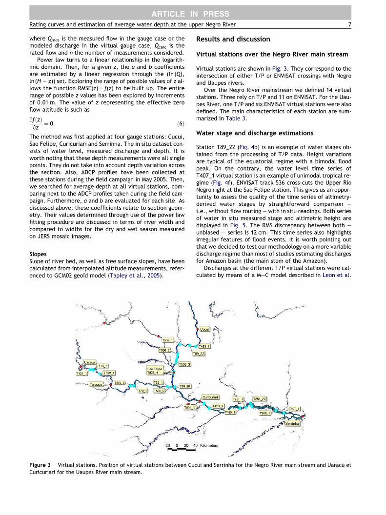
where Qmes is the measured flow in the gauge case or themodeled discharge in the virtual gauge case, Qcalc is therated flow and n the number of measurements considered.
Power law turns to a linear relationship in the logarith-mic domain. Then, for a given z, the a and b coefficientsare estimated by a linear regression through the (ln(Q),ln (H z)) set. Exploring the range of possible values of z al-lows the function RMSE(z) = f(z) to be built up. The entirerange of possible z values has been explored by incrementsof 0.01 m. The value of z representing the effective zeroflow altitude is such as
ofðzÞ
oz¼ 0. ð6Þ
The method was first applied at four gauge stations: Cucui,Sao Felipe, Curicuriari and Serrinha. The in situ dataset con-sists of water level, measured discharge and depth. It isworth noting that these depth measurements were all singlepoints. They do not take into account depth variation acrossthe section. Also, ADCP profiles have been collected atthese stations during the field campaign in May 2005. Then,we searched for average depth at all virtual stations, com-paring next to the ADCP profiles taken during the field cam-paign. Furthermore, a and b are evaluated for each site. Asdiscussed above, these coefficients relate to section geom-etry. Their values determined through use of the power lawfitting procedure are discussed in terms of river width andcompared to widths for the dry and wet season measuredon JERS mosaic images.
Slopes
Slope of river bed, as well as free surface slopes, have beencalculated from interpolated altitude measurements, refer-enced to GCM02 geoıd model (Tapley et al., 2005).
Results and discussion
Virtual stations over the Negro River main stream
Virtual stations are shown in Fig. 3. They correspond to theintersection of either T/P or ENVISAT crossings with Negroand Uaupes rivers.
Over the Negro River mainstream we defined 14 virtualstations. Three rely on T/P and 11 on ENVISAT. For the Uau-pes River, one T/P and six ENVISAT virtual stations were alsodefined. The main characteristics of each station are sum-marized in Table 3.
Water stage and discharge estimations
Station T89_22 (Fig. 4b) is an example of water stages ob-tained from the processing of T/P data. Height variationsare typical of the equatorial regime with a bimodal floodpeak. On the contrary, the water level time series ofT407_1 virtual station is an example of unimodal tropical re-gime (Fig. 4f). ENVISAT track 536 cross-cuts the Upper RioNegro right at the Sao Felipe station. This gives us an oppor-tunity to assess the quality of the time series of altimetry-derived water stages by straightforward comparison –i.e., without flow routing – with in situ readings. Both seriesof water in situ measured stage and altimetric height aredisplayed in Fig. 5. The RMS discrepancy between both –unbiased – series is 12 cm. This time series also highlightsirregular features of flood events. It is worth pointing outthat we decided to test our methodology on a more variabledischarge regime than most of studies estimating dischargesfor Amazon basin (the main stem of the Amazon).
Discharges at the different T/P virtual stations were cal-culated by means of a M–C model described in Leon et al.
Figure 3 Virtual stations. Position of virtual stations between Cucui and Serrinha for the Negro River main stream and Uaracu et
Curicuriari for the Uaupes River main stream.
Rating curves and estimation of average water depth at the upper Negro River 7
ARTICLE IN PRESS

(submitted for publication) and the example of the dischargetime series for Virtual Station T89_22 is shown in Fig. 4a. Inthese examples, discharge variations are clearly related towater levels variations. Despite the short measurementsperiod for ENVISAT, the annual cycle of water levels is alsoclearly monitored, and discharge is correctly simulated bythe model (Fig. 4a–d). Similar results have been obtainedfor all stations. Rating curves have been computed accordingto the methodology described above for all stations.
Rating curve and water depth estimation
Before estimating rating curves and water depth at each vir-tual station, we tested the method at four different in situgauged stations: Cucui, Sao Felipe, Curicuriari and Serrinha.Similarly, we also validated the ADCP measurements atthese stations in May 2005. The water stage given by thethree methods, single-point measurement (GWD), averagedepth along the ADCP profile (MWD), and reference depthfor the rating curve (EWD) are reported in Table 4. It isworth noting that all stages in Table 4 are related to thesame discharge as measured by ADCP in May 2005. In Table4, D1 stands for the difference between GWD and MWD.That D1 is not zero highlights the variability of in situ esti-mates for the reach depth, that can exceed 20%. For all sta-tions, D2, that stands for the difference between GWD andMWD, is of the same order of magnitude as D1, and evensmaller than D1 in three cases. The mean absolute differ-ence between ADCP measured water depth and estimatedzero flow water depth at these four stations is 68 cm, i.e.,6% of mean depth.
Table 5 lists the results of the computed rating curve atthe 21 virtual stations taken into account in this study.
Reliability assessment of the rating curves
parameters
Correlation coefficients for all rating curves are adequatefor the ENVISAT virtual stations (Fig. 6). On the other hand,correlation coefficients found for the T/P virtual stationsare below 0.8, thus pointing to a higher dispersion of thealtimeter data (Fig. 6c and e). T/P data are known to bemore scattered than ENVISAT ones over rivers (Frappartet al., 2006) since the T/P ranges are estimated only withan ‘‘ocean-like’’ tracker when the best performing tracker,e.g., ICE-1 (Bamber, 1994), could be selected among fourfor the ENVISAT ranges. As a result, the T/P altimetric datascattering turns the rating-curve difficult to adjust and thisdirectly affects a and b coefficients and the reliability ofestimated effective zero flow.
With the exception of station T89_26, all b values re-ported in Table 5 are below 2 indicating that the stage–dis-charge relationships are mostly channel-controlled at thestudied virtual stations. As mentioned above, channel con-trol is expected in a portion of the river where the geometryand roughness of a long reach of channel downstream fromthe gaging station are the elements that govern the rela-tionship between stage and discharge.
Stations T89_26 yields a value of b greater than 2 indicat-ing a stage to discharge relationship governed by a closedownstream section. As reported in Fig. 3, this station is sit-uated at Uaupes River and Negro River confluence. In this
Table 3 Principal characteristics of the virtual stations
Station River Latitude/longitude Type of data Dry/wet season
cross-section
width (km)
Discharge
measured by
ADCP in
05/2005
(m3/s)
Average water
depth by ADCP
in 05/2005 (m)
Upstream In situ
station distance
(km)
T493_1 Negro 0.87/66.89 ENVISAT 1.72/2.23 7071 8.23 Cucui (47)
T89_22 Negro 0.91/67.00 T/P 1.4/2.08 7071 8.40 Cucui (60)
T536_1 Negro 0.92/67.19 ENVISAT 0.76/1.29 7623 10.18 Cucui (85)
T536_2 Negro 0.72/67.23 ENVISAT 1.02/1.98 8582 11.43 Cucui (113)
T536_3 Negro 0.60/67.26 ENVISAT 0.98/2.19 8647 9.32 Cucui (128)
T536_4 Negro 0.37/67.31 ENVISAT 1.06/2.19 11,625 12.24 Sao Felipe (0)
T89_26 Negro 0.09/67.29 T/P 0.8/0.84 12,524 11.95 Sao Felipe (33)
T994_1 Negro 0.23/66.73 ENVISAT 1.12/1.52 18,590 12.92 Curicuriari (10.6)
T493_2 Negro 0.33/66.62 ENVISAT 2.16/2.48 18,569 11.49 Curicuriari (26.5)
T450_1 Negro 0.32/66.03 ENVISAT 3.65/3.65 20,361 7.58 Curicuriari (100)
T951_1 Negro 0.31/65.91 ENVISAT 1.81/2.06 20,445 11.10 Curicuriari (114)
T254_22 Negro 0.24/65.81 T/P 2.72/7.70 21,841 11.48 Curicuriari (126)
T908_1 Negro 0.37/65.32 ENVISAT 2.91/2.91 22,388 12.44 Curicuriari (188)
T407_1 Negro 0.41/65.15 ENVISAT 2.44/2.44 23,460 11.78 Curicuriari (207)
T121_1 Uaupes 0.43/68.94 ENVISAT 0.8/1.29 No data No data Uaracu (50.3)
T178_7 Uaupes 0.43/68.89 T/P 0.98/0.98 No data No data Uaracu (57)
T622_1 Uaupes 0.35/68.75 ENVISAT 1.06/1.69 No data No data Uaracu (80.4)
T579_1 Uaupes 0.12/68.16 ENVISAT 1.21/2.64 4850 5.48 Taracua (60)
T78_1 Uaupes 0.11/68.09 ENVISAT 1.42/1.42 4791 6.13 Taraqua (69)
T35_1 Uaupes 0.11/67.45 ENVISAT 0.89/1.41 5190 8.98 Taraqua (160)
T536_5 Uaupes 0.09/67.36 ENVISAT 1.02/1.34 5204 10.6 Taraqua (168)
8 J.G. Leon et al.
ARTICLE IN PRESS

case, a section control might be expected. As discussed be-low, this b value greater than 2 can be also due to a down-ward break in bed slope at this section.
Based on Eq. (4) one can infer that values of coefficient ain Table 5 are strongly associated with three characteristicsof the channel control: friction slope (S), Manning roughnesscoefficient (n) and mean width of cross-section (W). Formost stations studied, the variations of a along the reachesare consistent with cross-section changes, slope changesand tributary inputs. Also, in station T254_22 a high valuewas found for a (1576). However, as reported in Table 3,this station features a 7 km width cross-section value duringthe rainy season. This characteristic, based on Eq. (4), leadsto a high value for the coefficient a.
Reliability of the estimated zero flow depth
compared with in situ depth measurements
Fig. 7 shows the evolution of RMS in discharge for somecross-sections when discharge–height pairs are fitted by arating curve for successive values of reference depth z.
Figure 4 Discharge and water stage time series. Discharge and water stage time series of three virtual stations along the Negro
River main stream.
20/11/32
30/20/10
30/40/21
30/60/12
30/80/03
30/11/80
40/10/71
40/30/72
-5.0
-2.5
0.0
2.5
5.0
7.5Sao Felipe measured water stage
T536_4 altimetry data
Date
He
igh
tm(
m( )e
an
r e
mo
ve
d)
Figure 5 Time series of water stage at Sao Felipe. The thin
continuous line stands for the daily in situ readings. ENVISAT
heights (black dots) are reported as the median value at each
pass (every 35 days) along with the standard deviation.
Rating curves and estimation of average water depth at the upper Negro River 9
ARTICLE IN PRESS

The minimum in RMS is always unique and well-defined. Bycomparing the results between estimated water depth andmeasured water depth in Table 5 we obtain an absolutemean difference of 1.2 m for all stations in Negro Riverand 0.67 m for those located on the Uaupes River. Themethod proposed seams rather robust and reliable, giventhe good agreement between measured and estimateddepths.
ADCP cross-section profiles for each virtual station to-gether with different estimates of mean water depth areshown in Figs. 8–10. Station T89_22 is not shown becauseonly partial ADCP profile was available.
The profiles located between the Cucui and Sao Felipestations (T493_1 and T536_1), upstream from the Negroand Uaupes rivers confluence are given in Fig. 8. Except
for station T536_1, it can be seen that the bottom irregular-ity of these sections is reduced and the depth can be reason-ably approximated by some equivalent average value. Inparticular, a 380 m long island is evidenced along the sec-tion of the T493_1 virtual station (Fig. 8a). ADCP profilescollected from the confluence to Serrinha station (Fig. 9)differ substantially from the upstream ones. These profilesare very irregular and depth varies largely within eachcross-section, especially for T89_26, T994_1, T450_1 andT951_1 stations. There, the characterization of the cross-section depth by a single value is less relevant. This findingis quantified at first-order by parameter rd reported in Table5 which stands for depth variability along the ADCP profile.Indeed, variability of ±7 m in MWD at T89_26 station for anaverage depth of 11.95 m or ±8.3 m at T951_1 station for
Table 4 Results of the method application at three gauged stations
Station a b R2 EWD (m) GWD (m) D1 (m) D2 (m) Difference between D1 and D2
Cucui 314.21 1.502 0.99 7.99 9.82 1.83 2.12 0.29
Sao Felipe 179.08 1.86 0.97 11.53 11.75 0.22 0.19 0.41
Curicuriari 33.13 2.495 0.96 13.6 11.03 2.57 0.73 1.84
Serrinha 105.73 2.308 0.94 10.83 11.78 0.95 0.77 0.19
GWD, gauged water depth at in situ station for the same discharge measured by the ADCP in 05/2005; EWD, estimated water depth by therating curve for the same discharge measured by ADCP; D1, difference between GWD and EWD; D2, difference between GWD and MWD.
Table 5 Results of the rating-curve and water depth estimations at virtual stations
Station a b z (m) R2 n Average
estimated
water depth
EWD (m) Difference between
MWD and EWD (m)
rd (m)
T493_1 594.08 1.26 70.04 0.98 17 4.68 7.26 0.97 1.38
T89_22 339.83 1.25 67 0.66 86 8.85 8.28 0.12 1.48
T536_1 412.92 1.35 68.80 0.99 16 6.07 8.66 1.52 3.48
T536_2 105.21 1.79 65 0.90 19 8.25 11.74 0.3 3.00
T536_3 206.56 1.63 66.34 0.98 18 6.85 10.05 0.72 1.61
T536_4 179.08 1.86 65.29 0.97 18 8.38 10.95 1.30 4.1
T89_26 115.64 2.01 59.5 0.79 98 9.64 9.01 2.94 7.04
T994_1 204.92 1.87 36.51 0.99 15 8.12 11.01 0.72 5.45
T493_2 257.14 1.79 35.90 0.98 15 8.04 10.80 0.69 3.76
T450_1 383.90 1.76 31.83 0.99 15 7.32 9.54 1.95 2.57
T951_1 422.10 1.73 30.29 0.99 15 6.93 9.42 1.68 8.3
T254_22 1576 1.001 25 0.76 94 10.23 11.87 0.39 4.67
T908_1 490.52 1.71 25.29 0.98 18 7.21 8.82 1.16 2.44
T407_1 553.80 1.67 24.67 0.99 15 7.01 9.37 2.41 4.54
T121_1 529.41 1.35 89.79 0.97 14 3.88 – No MWD data –
T178_7 340.95 1.41 88.29 0.72 59 4.23 – No MWD data –
T622_1 768.88 1.25 89.79 0.96 13 2.33 – No MWD data –
T579_1 175.80 1.71 73.97 0.99 13 4.55 6.78 1.28 2.69
T78_1 410.41 1.36 74.11 0.97 14 4.72 6.092 0.04 3.26
T35_1 298.13 1.26 66.17 0.95 16 6.25 9.69 0.71 3.94
T536_5 121.58 1.55 63.92 0.95 16 7.71 11.28 0.68 3.45
GWD, gauged water depth at in situ station for the same discharge measured by the ADCP in 05/2005; EWD, estimated water depth by therating curve for the same discharge measured by ADCP; MWD, measured average water depth by ADCP under each altimetric track in 05/2005; a, b, coefficients of the rating curve (Eq. (4)); z, estimated zero effective flow stage from the ellipsoid WGS84 by RMSE minimizationmethod; R2, correlation coefficient of the rating curve; n, number of points in the rating curve; rd, standard deviation of the depth alongthe ADCP profile.
10 J.G. Leon et al.
ARTICLE IN PRESS

9.41 m average depth confirms the irregularity of the bot-tom shape and how difficult it is to measure a reliable equiv-alent water depth. The significant differences (>1 m)between EWD and MWD at these sections can be relatedto this fact or to the quality of the altimeter data. Indeed,these stations are located in areas where satellite measure-ments can be contaminated by the topography or physicalcharacteristics of the river channel such as meanders, islandsystems and major confluences. More spatial data are re-
quired to reinforce and validate the rating-curves of thesevirtual stations. However, it can also be assumed that amean depth measured from ADCP could be in these casesless reliable than the estimation of effective zero flow va-lue. For the time being, it can only be stated that discrep-ancies are higher in the event of an irregular profile.
At the downstream end of the reach, between T254_22and T407 stations (Fig. 9b–d), the width section changesby 1.5 km between high and low waters. This significant
Figure 6 Estimated rating-curves. Example of estimated rating-curves for some virtual stations.
Rating curves and estimation of average water depth at the upper Negro River 11
ARTICLE IN PRESS

width variation could also account for the value of a foundin station T254_22.
Lastly, some cross-section profiles are given in Fig. 10 forthe Uaupes River. rd ranges from ±2.7 m at T579_1 stationand ±4 m at T35_1 station, for an average water depth of7 m. Again, irregularity at the cross-sections detrimentallyaffects the estimate of typical water depth.
As shown in Table 5, for all stations with ADCP profileEWD values were found that do not depart from MWD bymore than rd. Thus, it can be concluded that the methodpresented in this study provides reliable estimates EWD ofthe equivalent zero flow from remote discharges and altim-eter data.
Bottom slope compared with free surface slope
during low and high water stages
The average bottom slope of the upper Negro River basincan be calculated on the basis of the zero effective flowestimations presented in Table 5 (Fig. 11). For the reachfrom T493_1 station to T536_4 station, upstream from theconfluence with Uaracu River, we computed a bed slopeof 4.56 · 105 m m1. From T89_26 station to 994_1 station,downstream from the confluence, the bed channel of theriver shows a major increase in bottom slope, namely2.4 · 104 mm1. This section of the river is so-called Sao
Gabriel da Cachoeira (Sao Gabriel Waterfall). With a denser
Figure 8 ADCP profiles from Cucui to Sao Felipe station (following down the Rio Negro). Measured profiles by ADCP in May 2005 for
the virtual stations located between Cucui and Sao Felipe.
T493_2
313233343536373839
450
550
650
750
850
950
z (m)
mrs
m( 3
s/)
T908_1
1921232527600
700
800
900
z (m)
mrs
( m
3s/)
T178_7
8384858687888990
720
740
760
780
800
820
840
860
z (m)
mrs
m( 3
s/)
T536_5
5960616263646566315
320
325
330
335
340
z (m)
mrs
m( 3
s/)
Figure 7 RMS evolution. Evolution of the RMS in discharge when the discharge–height pairs are fitted by a rating curve for
successive values of the reference depth z.
12 J.G. Leon et al.
ARTICLE IN PRESS

network of stations due to the addition of virtual stations,the method even allows us to track the major changes inbed slope. Finally, a bed slope of 6.86 · 105 mm1 is foundfor the most downstream reach of the upper Negro Rivermain stream.
Similarly, the Uaupes River bed slope was estimated fromstations T121_1 to T536_5 (Fig. 12). An average slope of1.02 · 104 mm1 was calculated for this reach. A majorchange in slope was found between T622_1 and T579_1 vir-tual stations.
These results can be compared with the free water sur-face slope calculated from ENVISAT altimetry data. Fig. 13shows the profile of free water slope in dry season, rain sea-son and the bottom slope of the upper Negro River betweenT536_1 and T407_1 ENVISAT virtual stations. A very goodagreement is found between the free surface slope and
the bottom slope, providing an external validation of thismethod for water depth estimation at virtual stations. Theagreement between the free surface and bed slopes alsovalidates the assumption we made of kinematic slope.
Estimation of Manning roughness coefficient
Combining the Manning equation (1) and rate to dischargerelationship equation (4), the Manning roughness coefficient(n) can be derived from known values of a, S and W. Meanbottom slope values were used from T493_1 to T536_4 vir-tual stations, T89_26 to T994_1, 493_2 to 254_22, andT908_1 and 407_1 for the Negro River main stream. Width(W) values were estimated using JERS images acquired dur-ing the dry and rainy seasons. Thus, the n values were esti-mated at the different reaches with the same physical
Figure 9 ADCP depth profiles at the virtual stations (following the Rio Negro, from Sao Felipe to Serrinha). Profiles collected in
May 2005.
Figure 10 Uaupes River profiles. Measured profiles by ADCP in May 2005 for the virtual stations located at Uaupes River main
stream.
Rating curves and estimation of average water depth at the upper Negro River 13
ARTICLE IN PRESS
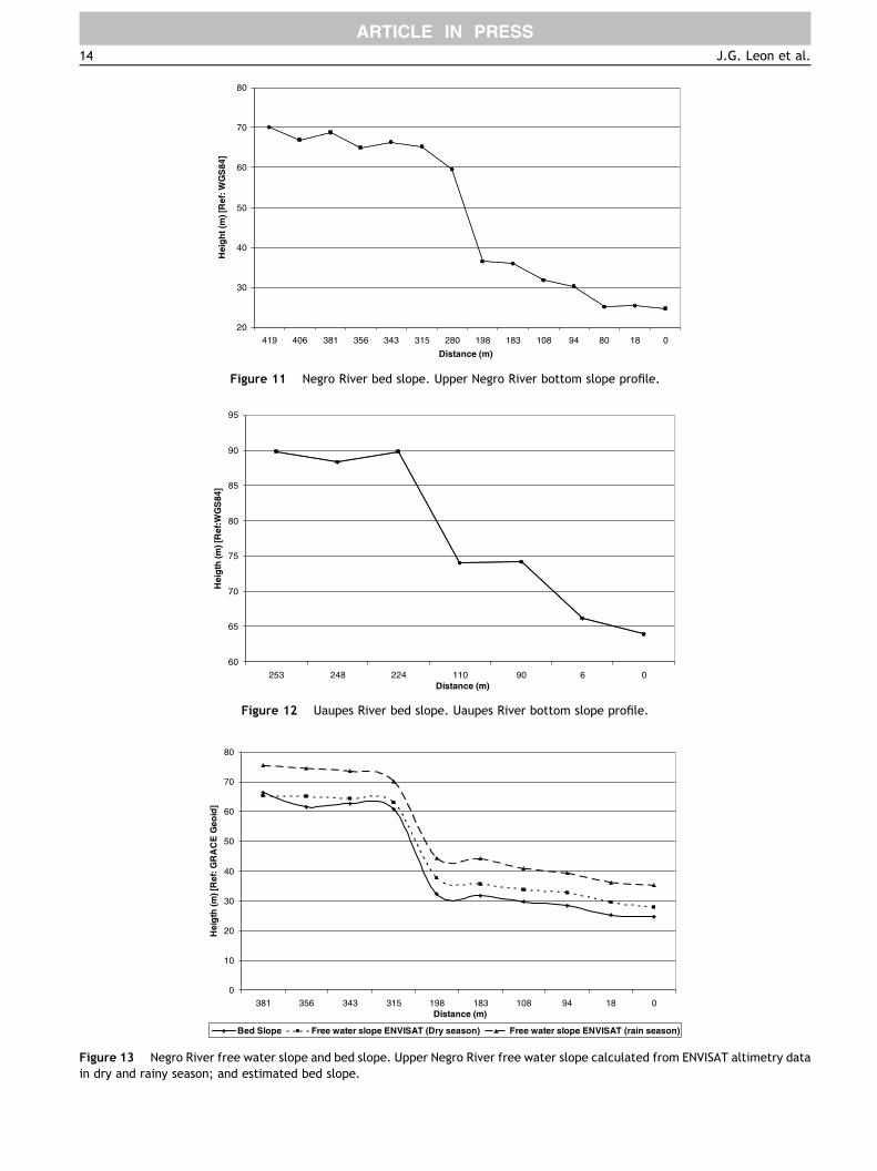
60
65
70
75
80
85
90
95
253 248 224 110 90 6 0
Distance (m)
He
ight
(m)
R[e
fW:
GS
84
]
Figure 12 Uaupes River bed slope. Uaupes River bottom slope profile.
0
10
20
30
40
50
60
70
80
381 356 343 315 198 183 108 94 18 0
Distance (m)
eH
igth
(m)
[Re
f:G
GE
CA
Re
oid
]
Bed Slope Free water slope ENVISAT (Dry season) Free water slope ENVISAT (rain season)
Figure 13 Negro River free water slope and bed slope. Upper Negro River free water slope calculated from ENVISAT altimetry data
in dry and rainy season; and estimated bed slope.
20
30
40
50
60
70
80
419 406 381 356 343 315 280 198 183 108 94 80 18 0
Distance (m)
He
gih
t(m
)R[
ef:
WG
S8
4]
Figure 11 Negro River bed slope. Upper Negro River bottom slope profile.
14 J.G. Leon et al.
ARTICLE IN PRESS

characteristics considering changes in slope, and the pres-ence of the island systems. For the Uaupes River, we onlyconsidered one average bottom slope from T121_1 to536_5. Table 6 summarizes the resulting Manning coefficientvalues found for these reaches during the dry and rainseasons.
Values of roughness coefficient reported in Table 6 areconsistent with values suggested by Chow (1959). For majorflows (width >30 m) with an irregular section, Chow (1959)suggests that Manning’s coefficient ranges from 0.035 to0.1. The highest values correspond to irregular naturalchannels with significant variations in cross-section, majorobstructions, and the presence of vegetation, meandersand islands. Values reported in Table 6 indicate that the Ne-gro River behaves as channels with irregular and roughnesssection in reaches 1, 3 and 4 with an n mean value betweendry and rainy season of 0.036 and of 0.049, respectively.Similarly, the Uaupes River (reach 5) has a mean n valueof 0.045 suggesting physical characteristics similar to thoseof the Negro River. On the other hand, higher values of n areobtained in reach 2. As discussed above, the stations consid-ered are located in a river portion of complex geometry di-rectly impacting hydrodynamics. As indicated in Chow(1959), a strong slope, meanders and islands lead to highervalues of n.
Conclusions
This work highlights a very promising application of the spa-tial altimetry over inland waters, especially over the greatfluvial basins such as the Amazon basin, but in areas withinthis basin where both geometry and discharge are veryirregular (upstream reaches of Rio Negro sub-basin). Theestimation of the stage–discharge relationship at virtualstations with a high accuracy from calculated remote dis-charges and filtered altimeter data are a new field in thespatial hydrology. We estimated the rating-curves for 21 vir-tual stations at the upper Negro River basin: 14 along theNegro River main stream between Cucui and Serrinhagauged stations and 7 along the Uaupes River from Uaracustation to the confluence with Negro mainstream (Fig. 3).
The RMSE minimization method presented in this paperhas allowed us to estimate the zero effective flow and con-sequently the water depth of these 21 cross-sections withan average difference less than 1.1 m between measuredwater depth and estimated water depth. It can be statedthat the preliminary results and the performance of themethod are reliable. This is supported by EWD values lyingwithin one standard deviation from the MWD. Using the rat-
ing curves obtained at the successive virtual stations al-lowed us to estimate consistent Manning roughnesscoefficients have been estimated and we determined theflow propagation conditions (either channel or section con-trolled). Our method allows us to extract bottom elevation,bottom and free surface slopes and roughness coefficientsfrom a combination of altimeter and remote discharge data.These quantities are highly valuable for understanding riversand hydrodynamic modelling. The methodology developedshould support future work on the Amazon Basin wherehydrodynamic modelling had always been prevented bythe lack of in situ data.
Acknowledgements
This study was funded by the CASH project from the ‘‘Re-seau Terre & Espace’’ of the French Ministry of Researchand Technology (MR decision No. 04 T 131), and by the ECCOPNRH MESBAM project. We are very grateful to the review-ers of this work, for their helpful remarks. We address spe-cial thanks to Gerard Cochonneau, who is in charge of theHybam in situ database and is always more than helpful bysharing his great experience in discharge data processingand stage to discharge relationship computing. Finally, ourthanks are addressed to Jean Loup Guyot for the passionatediscussions about the measurement of river bed from space.
References
AVISO User Handbook, 1996. Merged TOPEX/Poseidon Products(GDR-Ms), AVI-NT-02-101-CN, Edition 3.0.
Bamber, J.L., 1994. Ice sheet altimeter processing scheme. Int. J.Remote Sensing 15 (4), 925–938.
Barrett, E., 1998. Satellite remote sensing in hydrometry. In:Herschey (Ed.), Hydrometry: Principles and Practices, seconded. Wiley, Chichester, pp. 199–224.
Berry, P.A., 2003. Global river and lake monitoring from multimis-sion altimetry: capability and potential. In: The Abstracts of theWorkshop Hydrology from Space, 29 September–1 October2003, Toulouse, France.
Birkett, C.M., 1995. The contribution of Topex/Poseidon to theglobal monitoring of climatically sensitive lakes. J. Geophys.Res. 100 (C12), 25179–25204.
Birkett, C., 1998. The contribution of TOPEX NASA radar altimeterto the global monitoring of large rivers and wetlands. WaterResour. Res. 34, 1223–1239.
Birkett, C.M., Mertes, L.A., Dunne, T., Costa, M., Jasinski, J., 2002.Altimetric remote sensing of the Amazon: application ofsatellite radar altimetry. J. Geophys. Res. 107 (D20), 8059.doi:10.1029/2001JD000609.
Birkhead, A., James, C., 1998. Synthesis of rating curves from localstage and remote discharge monitoring using nonlinear Muskin-gum routing. J. Hydrol. 205, 52–65.
Bjerklie, D.M., Dingman, S.L., Vorosmarty, C.J., Bolster, C.H.,Congalton, R.G., 2003. Evaluating the potential for measuringriver discharge from space. J. Hydrol. 278 (14), 17–38.
Boroughs, C., Zagona, E., 2002. Daily flow routing with theMuskingum–Cunge method in the Paecos River Riverware Model.In: Proceedings of the Second Federal Interagency HydrologicModeling Conference, Las Vegas, NV, July.
Cazenave, A., Bonnefond, P., DoMinh, K., 1997. Caspian Sea levelfrom Topex/Poseidon altimetry: level now falling. Geophys. Res.Lett. 24, 881–884.
Table 6 Manning roughness coefficient along the Negro and
Uaupes Rivers
Reach Reach
number
n
(dry season)
n
(rain season)
T493_1–T536_4 1 0.04 0.076
T89_26–T994_1 2 0.093 0.11
T493_2–T254_22 3 0.037 0.04
T908_1–T407_1 4 0.032 0.032
T121_1–T536_5 5 0.036 0.054
Rating curves and estimation of average water depth at the upper Negro River 15
ARTICLE IN PRESS

Chow, V.T., 1959. Open Channel Hydraulics. McGraw-Hill, New York.Chow, V.T., Maidment, D., Mays, L., 1988. Applied Hydrology.
McGraw-Hill, New York.Coe, M., Costa, M., Botta, A., Birkett, C.M., 2002. Long-term
simulations of discharge and floods in the Amazon Basin.Geophys. Res. 107 (D20). doi:10.1029/2001JD000740.
Cunge, J.A., 1969. On the subject of a flood propagation computationmethod (Muskingum method). Hydraul. Res. 7 (2), 205–230.
Dubroeucq, D., Volkoff, B., 1998. From oxisols to spodosols andhistosols: evolution of the soil mantles in the Negro River basin(Amazonia). Catena 32, 245–280.
Frappart, F., Calmant, S., Cauhope, M., Seyler, F., Cazenave, A.,2006. Preliminary results of ENVISAT RA-2-derived water levelsvalidation over the Amazon Basin. Remote Sens. Environ. 100(2), 252–264.
Guyot, J.L., 1993. Hydrogeochimie des fleuves de l’AmazonieBolivienne. In: Geologie, Geochimie, Universite Bordeaux I,Bordeaux, p. 261 (in French).
Jasinski, M.J., Birkett, C.M., Chinn, S., Costa, M.H., 2001. In:Abstract, NASA/NOAA GAPP and Hydrology Principal Investiga-tors Meeting, April 30–May, Potomac, MD.
Johnson, D.,Miller, A., 1997. A spatially distributed hydrologicmodelutilizing raster data structures. Comput. Geosci. 23 (3),267–272.
Leon, J.G., Bonnet, M.P., Cauhope, M., Calmant, S., Seyler, F.,submitted for publication. Distributed water flow estimates ofthe upper Negro River using a Muskingum–Cunge routing modelbased on altimetric spatial data. J. Hydrol.
Merkel, W., 1999. Muskingum–Cunge Flood Routing Procedure inNRCS Hydrologic Models. USDA NRCS, National Water andClimate Center, Beltsville.
Ponce, V.M., 1986. Diffusion wave modelling of catchment dynam-ics. J. Hydraul. Div., ASCE 112 (8), 716–727.
Ponce, V.M., Lohani, A., Scheyhing, C., 1996. Analytical verificationof Muskingum–Cunge routing. J. Hydrol. 174, 235–241.
Rantz, S.E. et al., 1982. Measurement and computation of stream-flow. Measurement of Stage and Discharge, US Geological SurveyWater Supply Paper, vol. 1, p. 284.
Renellys, C. Perez, Dudley, B. Chelton, Robert, N. Miller, 2005. Theeffects of wind forcing and background mean currents on thelatitudinal structure of equatorial Rossby waves. J. Phys.Oceanogr. 35 (5), 666–682.
Richey, J., Mertes, A., Dunne, T., Victoria, R., Forsberg, B.,Tancredi, A., Oliveira, E., 1989. Sources and routing of theAmazon River flood wave. Global Biochem. Cycl. 3 (3), 191–204.
Soil Survey Staff, 1975. Soil Taxonomy. Basic System of SoilClassification for Making and Interpreting Soil Surveys. USDA,Washington, Agricultural Handbook 436, 754 pp.
Soil Survey Staff, 1990. Keys to Soil Taxonomy. Agency forInternational Development. USDA Soil Management SupportServices. Technical Monograph 19, fourth ed., Virginia Poly-technic Institute and State University.
Tapley, B., Ries, J., Bettadpur, S., Chambers, D., Cheng, M., Condi,F., Gunter, B., Kang, Z., Nagel, P., Pastor, R., Pekker, T., Poole,S., Wang, F., 2005. GGM02 – An improved Earth gravity fieldmodel from GRACE. J. Geodesy 79 (8), 467–478.
16 J.G. Leon et al.
ARTICLE IN PRESS