Hydrological management of a heavily dammed river basin ...€¦ · Hydrological management of a...
29
[email protected] www.eforenergy.org ISSN nº WP 03/2014 Hydrological management of a heavily dammed river basin: the Miño-Sil Juan A. Añel Mohcine Bakhat Xavier Labandeira
Transcript of Hydrological management of a heavily dammed river basin ...€¦ · Hydrological management of a...

WP 03/2014
Hydrological management of aheavily dammed river basin: theMiño-Sil
Juan A. AñelMohcine BakhatXavier Labandeira
Hydrological management of a heavily dammed river basin: the Miño-Sil
Juan A. Añel1,2,3, Mohcine Bakhat3, Xavier Labandeira3,4,5
1 Smith School of Enterprise and the Environment, University of Oxford, OUCE, South Parks Road, OX13QY Oxford (UK)
2 EphysLab, Facultade de Ciencias, Universidade de Vigo, Campus As Lagoas, 32004 Ourense (Spain)
3 Economics for Energy, Doutor Cadaval 2, 3E, 36202 Vigo (Spain)
4 Rede, Universidade de Vigo, Facultade de CC.EE., Campus As Lagoas, 36310 Vigo (Spain) 5 FSR-Climate, European University Institute, Via delle Fontanelle 19, 50014 Firenze (Italy)
Abstract
We herein research the potential environmental impacts of the management of dams in the Miño-Sil river basin on the natural flow of their rivers. The Miño-Sil is a transnational river basin in the north-western Iberian Peninsula, and is managed by Spanish authorities. The basin is heavily managed with more than 100 dams, which in the main are used exclusively for hydropower generation. For the period of this study (1978-2012), we analyze the repercussions of the liberalization of the Spanish energy market in 1998. Our results show that the dams in the Miño-Sil river basin years had no influence on the natural river flows over the period of interest. Moreover, despite being used so heavily for hydropower, the liberalization of the Spanish energy market did not increase the degree of intervention in river flows. Indeed for three reservoirs in particular the correlation between inflow and outflow improved. It is also clear that for the reservoirs considered, the mean water storage and monthly inflows were lower during 1998-2012 than during 1978-1997.
Keywords: water management, reservoirs (surface) dams, hydroclimatology,
systems operation and management ___________________ Corresponding author: Juan A. Añel. Email: [email protected]. Phone: +44 (0)1865 614940 The authors would like to thank the Confederación Hidrográfica Miño-Sil (the Miño-Sil river Basin District Authority) for providing some of the data used for this study. We would also like to thank Carlos G. Ruiz (MSRBDA) and David A. Pérez (Gas Natural Fenosa) for their useful comments and help. The usual disclaimer applies. The funders had no role in the design of the experiments, analysis, or interpretation of results. This study was partly funded through a contract with the Gas Natural-Fenosa Chair at the Universidade de Vigo. The funder had no role in the research, the design of the experiments, or the analysis and interpretation of the results.

2
1. Introduction
The presence of a dam can significantly alter the hydrological characteristics of a catchment. They are
built for a range of purposes, including flood control, hydropower generation and water supply. Their
environmental impact depends on their use, on geophysical factors (meteorology, climatology), and on
their management strategies. There is a significant scientific literature on the effects of dams on floods
[e.g., López-Moreno et al., 2002], droughts [e.g., López-Moreno et al., 2009], and the environment [e.g.,
Garcia et al., 2011]. The common cause of all these phenomena is the alteration of natural flows as a
consequence of the existence and operation of dams [e.g., Botter et al., 2010]. Several authors have
correspondingly proposed the use of operating rules to minimize the negative effects of dams [Renöfalt et
al., 2010; Yin et al., 2011], although these may compromise other objectives pursued by dam builders
[Barlett et al. 2012].
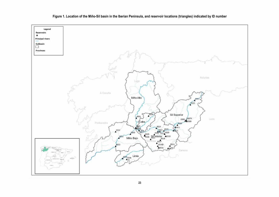
The 'Miño-Sil basin' is the common name for the area administered by the Miño-Sil River Basin District
Authority (MSRBDA). The area comprises the basins of the Miño, Sil, Cabe and Limia rivers, and is
divided into six different zones: Miño-Alto, Miño-Bajo, Cabe, Limia, Sil-Superior and Sil-Inferior (see Figure
1). The Miño-Sil is the fourth largest basin in the Iberian Peninsula in terms of annual mean flow (10570
hm3), and is thus important for hydropower generation [Lorenzo-Lacruz et al., 2012]. The Miño river flows
into the Atlantic Ocean: 95% of its basin is in Spain, but its last 76 km form the border with Portugal. The
Limia crosses the border with Portugal, while the Sil and Cabe lie entirely in Spanish territory. The
MSRBDA manages the Spanish sections of the Miño and Limia rivers, together with the transitional and
coastal waters shared with Portugal, under a bilateral agreement [Ministerio de Asuntos Exteriores y de
Cooperación, 2010].
The Miño-Sil basin is economically important for the region, in the tourism, fishing, agricultural and power
generation sectors. One main characteristic of the Miño-Sil basin is that most of the reservoirs are used
solely for hydropower generation, with just two also used for water supply or irrigation (see Table 1). There
are 106 hydroelectric stations in the basin, of which 36 are cataloged by the MSRBDA as 'big reservoirs'
on the basis of their total surface areas. In 2012 the installed generating capacity reached 2773 MW.
Water from the basin is also used by two thermal power plants with an installed capacity of 1629 MW,
bringing the basin’s gross annual production of electricity to 14143 GWh, constituting 8.58% of the Iberian
Peninsula’s total electrical installed power [Confederación Hidrográfica del Miño-Sil, 2012] (information
available online in www.chminosil.es). Several further projects have recently been finished or are under
development to increase hydropower generation, including pumped storage reservoirs for use with
existing local wind power plants.

3
For such a complex and heavily modified basin [Martínez-Gil and Soto-Castiñeira, 2006], one which
already contributes a major share of Spanish electricity generation capacity and which is due to be
increased through the addition of further hydropower projects, it is very important to gain a quantitative
insight into its management from an environmental point of view in order to understand the effects of
hydropower as mentioned above. Accordingly, in 2009 the regional government of Galicia, where most of
the dams in the Miño-Sil basin are located, introduced a tax on hydropower production. Even though the
tax was probably aimed at capturing the hypothetical rents associated with hydroelectric generation [see
Gago et al., 2013], it may also have reflected environmental concerns.
The operation of a hydropower system depends primarily on the availability of water resources (runoff),
but it also depends on other technical guidelines (for example those provided by the operator of the grid)
and the economic factors related to the alternatives to hydropower generation. In the face of scarce or
non-existent information on these secondary aspects, the potential changes in electricity generation from
existing hydropower plants can be considered to be a consequence of the impact of climate change for a
country or region.
Instead of a single managing body, the Miño-Sil basin relies on a mix of decisions made by public
authorities, including the MSRBD and Red Electrica de España (the operator of the Spanish electricity
system), and several independent private companies that use the hydropower stations (see Table 1). It is
likely that these decisions are motivated by a range of motivations, including economic factors, in addition
to the region’s climatology and hydrometeorology.
It has been shown that climatology is important, because of the link connecting the annual hydrological
cycle with phenomena such as the North Atlantic Oscillation (NAO) [García et al. 2005; Gimeno et al.
2001; Trigo 2011]. In addition to the usual effects of climatic variability on the region, climate change has
affected fresh water resources via changes in the hydrological cycle. The last report by the
Intergovernmental Panel on Climate Change [IPCC, 2013] supported the proposition of a positive trend in
precipitation for mid-latitude areas of land in the northern hemisphere. Bates et al. [2008] argued that the
changes will be widespread and that: a) the quantity, variability, timing, form, and intensity of precipitation
and annual average runoff will change, b) the frequency and intensity of extreme events such as floods
and droughts will rise, c) water temperatures and the rate of evaporation will increase, and d) water quality
in rivers and lakes will deteriorate. Despite international agreement on the threat of climate change to
water resources, the nature and magnitude of these impacts are deemed to be country/region-specific.
Some regions are expected to receive too much or too little water, with a higher variability in precipitation
and river discharge projected to cause great damage due to an increase in floods and droughts. These
problems will be further exacerbated in the second half of the 21st century [Bates et al., 2008].

4
Mukheibir [2013] makes a distinction between long-term impacts related to trends, and short-term impacts,
which are usually linked with extreme weather events. Long-term variations in rainfall patterns could cause
highly variable inflows to reservoirs, and have the potential to affect hydropower generation. This could
cause the operation of some dams to become sub-optimal, either for technical or economic reasons [Iimi,
2007]. This effect could be exacerbated by increased evaporation due to the expected increase in mean
global temperature, reducing reservoir water levels. Hamududu and Killingtveit [2012] states that by 2050,
climate change will lead to a 1.73 TWh/yr (1.28%) decrease in hydropower production in western Europe,
being up to 10% for Spain. It also states that the impacts will differ by region and must therefore be
studied at a local level.
By the end of the 21st century, the water resources available for hydropower production in the Miño-Sil
basin will be at best 40% less than those available for the period 1980-1999 [IPCC, 2011] . Lehner et al.
[2005] predicted that by 2070, electricity production from southern European hydropower stations would
be reduced by 20–50% in comparison with the period 1960-1990. Spanish hydropower generation in
recent years is believed to be below historical levels for most plants, due to a series of dry years on the
Peninsula [Espejo and García-Marín, 2010]. While the annual inflow generally determines the total
hydropower generation [Tanaka et al., 2006], hydropower endowments can also be affected by the impact
of climate change on the seasonal pattern of the hydrological cycle. In Spain, the majority of hydropower
plants were built in the 1960s, in locations that were chosen based on historical records of climatic
patterns that are now obsolete as a result of natural climate variability.
The research presented here is informed by a dual interest in environmental impacts: those resulting from
dam operations in the Miño-Sil basin, and those related to the liberalization of the Spanish energy market.
In 1998 the Spanish electricity sector went through a major transformation in the interests of this process
of liberalization; this could well have affected the management strategies of the different reservoirs in the
basin. We therefore split the study into two periods, before and after 1998.
We applied a number of different statistical tests together with a clustering technique to streamflow and
water storage time series from the Miño-Sil basin. The remainder of this paper is structured to include a
data and methods section, followed by the results for storage capacities, inflows, outflows, trends and
clustering analysis, and a discussion.

5
2. Data and Methods 2.1 Data Hydrological data were obtained from the MSRBDA. The hydrological data include the daily observed
discharge (streamflow) of mountain stations, and discharge from stations along the main tributaries of the
Miño and Sil rivers. Of the 36 big reservoirs in the Miño-Sil basin, 31 were included in this study. The
reservoirs selected were those with the longest time series that contained less than 5% missing values.
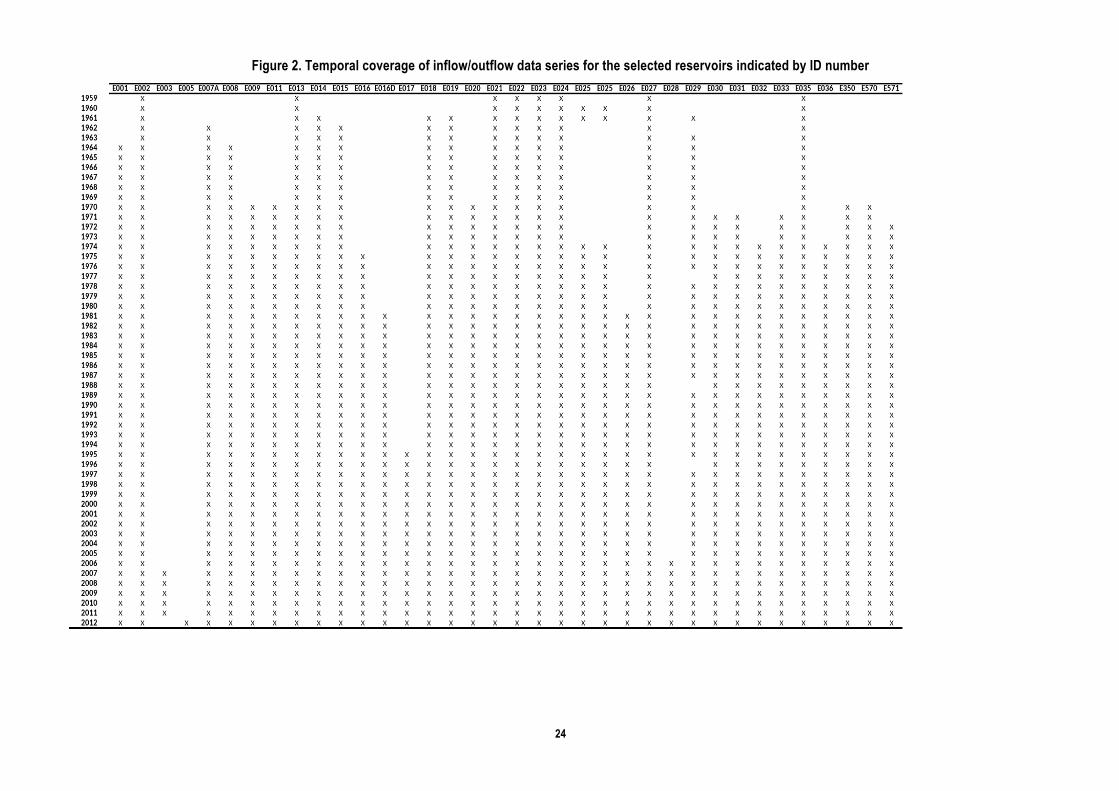
The study covers the period from 1978 to 2012, which is the maximum period of continuous data for
inflows and outflows. Although the data for two of the reservoirs (IDs 1780 and 1781) cover a shorter time
span, they were included because of their hydrological importance (for example, reservoir 1781 has the
lowest storage capacity). The temporal coverage of the data is summarized in Figure 2. The reservoirs’
locations are shown in Figure 1, and Table 1 lists additional hydrological information. The selected data
represent the main reservoirs distributed over the upstream and downstream sections of the area of study.
Unlike meteorological data, water storage data do not require specific tests to detect and correct
inhomogeneities [Morán-Tejeda et al., 2012]; such tests are not feasible because it is not possible to
establish the source of the inhomogeneity. In some cases where the data series of inflow was incomplete,
we gap-filled the series using the continuity equation that relates storage capacity (St), inflow (It), and
outflow (Ot): St=St-1+It-Ot [Martin et al., 1999 (page 432)]. The selected reservoirs are all used exclusively
for electricity generation, except for the Bárcena and Fuente del Azufre reservoirs (ID numbers 1709 and
1710 respectively), which are also used for irrigation and water supply, respectively.
To ensure the reproducibility of this research [Añel, 2011], our computations were performed using the
software R v2.15 [R Core Team, 2012], free software under the GPLv2 license
(http://www.gnu.org/licenses/old-licenses/gpl-2.0.html). The 'kendall', 'boot' and 'stats' packages were
used, in particular.
2.2 Impoundment ratio and correlation To measure the influence of each dam on its downstream hydrology we follow the methodology of Morán-
Tejeda et al. [2012] by computing the Impoundment Ratio (IR) and the Operational Impoundment Ratio
(OIR) [Batalla et al., 2004; Morán-Tejeda et al., 2012]. The two quantities differ in the numerator, which for
IR is 'storage capacity' and for OIR is the 'operational storage capacity', defined as the difference between
the historical maximum and the historical minimum of the storage capacity.

6
IR =Storage Capacity
Long! term Mean Annual Inflow
In order to assess the degree to which the river flow regimes were altered, we computed the Pearson’s
correlation coefficient between inflows and outflows. The correlation coefficient 'r' is a measure of the
rectilinear relationship between the variables, in which larger values correspond to stronger associations.
At its extreme, a correlation of 1 means that the river regime downstream of the reservoir was identical to
the regime at the reservoir entrance, so that there was no alteration of the natural flow regime. At the other
extreme, a negative correlation of value -1 indicates that high inflows are paired with low outflows, and
vice versa, indicating a reversal of the river’s natural seasonality. A correlation value |r|=0 implies an
absence of correlation between inflows and outflows, which also means a significant alteration to the river
flow regime [Batalla et al. 2004; Morán-Tejeda et al. 2012].
2.3 Trends and cluster analysis
To analyze the potential trends in storage capacities and monthly outflows during the study period we
used the following approaches: (i) a local polynomial regression fitting (LOESS) [Cleveland et al., 1993],
(ii) a simple linear regression analysis plus boostrapping, (iii) a non-parametric Mann-Kendall test.
Because the first two tests require normality, we used Q-Q-plots to check that this condition was fulfilled
by all of the series (see dynamic content 1). We note that all three variables (storage, inflow and outflow)
are normally distributed for all the reservoirs except Sequeiros, Montefurado, Frieira and San Martín (ID
numbers 1751, 1744, 1641 and 1740 respectively).
The LOESS procedure utilizes a nonparametric method to estimate regression surfaces and hence
identifies any long-term behavior in the data. Its use is suitable when outliers are detected in the data and
a robust estimation is needed.
We applied a linear regression directly to each of the time series in turn, using time as the independent
variable. When interpreting the slope of the regression line, trends may be obscured by data scatter
arising from multiple sources, including non-ideal hydrogeological conditions, and sampling
inhomogeneities. Even though the scatter may be large, yielding a low goodness-of-fit, the overall trends
in the data may still be ascertained using the confidence intervals. The null hypothesis H0 that there is no
trend is tested against the alternative hypothesis H1 that there is a trend at different significance levels
(1%; 5%; 10%).

7
To examine further the robustness of the linear trends, a bootstrapping analysis [Davison and Hinkley,
1997] with 1000 random samples was also performed. 1000 slopes were calculated and 95% confidence
intervals were derived from the normally distributed slopes, to indicate the extent to which the trends are
affected if the time series is relatively short.
Finally, as the selected time series in this study are not perfectly normally distributed, we also used the
non-parametric Mann-Kendall (MK) test [Kendall, 1975; Mann, 1945] to double-check the validity of the
results from the linear regression. The MK test is based on the rank-correlation approach, and has been
widely used in hydrometeorological studies to test the validity of the null hypothesis, of no trend, against
the alternative hypothesis of increasing or decreasing trend [Hamed, 2008; Fu, 2004; Moberg and Jones,
2005; Morán-Tejeda et al., 2012; Rotstayn and Lohmann, 2002; Zhang, 2009].
Clustering [Gordon, 1987; Everitt et al., 2011] allows observations to be grouped according to how similar
they are, on the basis of a measure of the distance between observations. Cluster analysis techniques fall
into three categories: agglomerative hierarchical techniques, k-means clustering, and k-medoids
clustering. Here we used all three methods.
For the hierarchical technique, we used the Euclidean distance between objects to form the clusters, and
Ward’s method to determine the similarity between objects [Ward, 1963], which has previously been
successfully tested [Bonell and Summer, 1992; Morán-Tejeda et al., 2012].
The k-means clustering algorithm also uses the Euclidean distance but minimizes the within-class sum of
squares from a pre-specified number of cluster centers [Ripley, 2002].
The k-medoids method is very similar to the k-means method. The main differences lie in the way the
center of a cluster is chosen, and that k-medoids clustering is more robust in the presence of outliers.
Here we use the CLARA algorithm for k-medoids clustering, an improvement on the Partitioning Around
Medoids (PAM) method, which improves the efficiency when clustering large data. In cases where the
data are not clearly separated into groups, identifying the number of clusters becomes more difficult. We
addressed this problem using validity indexes to measure the quality of each cluster, namely the wb,
Silhouette and Dunn’s indexes [Zhao, 2013].

8
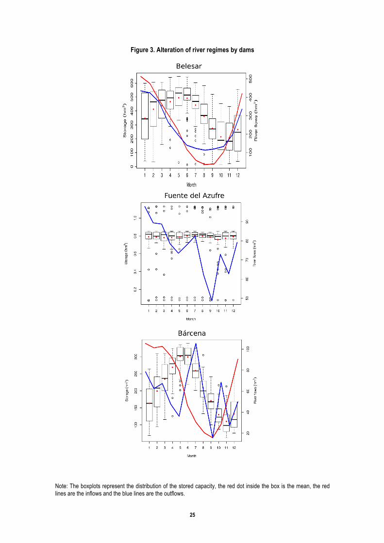
3. Results 3.1. Dam operations and river regimes We chose three different reservoirs with different uses and conditions to show the impacts of dam
operations and reservoir management (see Figure 3). Figures for the other reservoirs are included in
dynamic content 2.
The Belesar dam across the Miño River was completed in 1963 and is the largest in the Miño-Sil basin,
with a storage capacity of 654 hm3 and a generation capacity of 225 MW during the study period
(following construction work in November 2013 a further 20.8 MW were added). The reservoir shows high
flows between December and April, and low flows for May-November. The minimum (208 hm3) and
maximum (495 hm3) storage capacities are recorded in November and May, respectively. Figure 3 shows
that inflows exceeded outflows from November to May, while outflows exceeded inflows from June until
the end of summer season. The flows in the Belesar basin are only slightly altered by the presence of the
dam, as indicated by the high correlation coefficient (0.98).
In the Sil-Superior zone the Fuente del Azufre reservoir has a smaller storage capacity and is used for
hydropower and water supply. The monthly reservoir capacity has a small variation with a long-term
maximum capacity in July. The flows exhibit a different pattern, with inflows having two marked peaks
(note that in Figure 3 the inflow (red line) is not obvious as it is extremely similar to outflow (blue line)), one
in summer and the other in winter, and with water releases dropping markedly between January and May
and also between July and September. The very low storage capacity of this particular reservoir means
that its management strategy is intended to keep the storage capacity at a certain level without altering
river regimes. This is also shown by the high correlation coefficient of 1.
In the same Sil-Superior zone the Bárcena reservoir with 341 hm3 storage capacity is used for irrigation
and electricity generation. The monthly storage capacity reaches its maximum in May and its minimum in
November. The alteration of the river regime downstream of the reservoir is more pronounced than in the
previous two cases. This is confirmed by a smaller correlation coefficient between the monthly inflows and
outflows (r=-0.259).
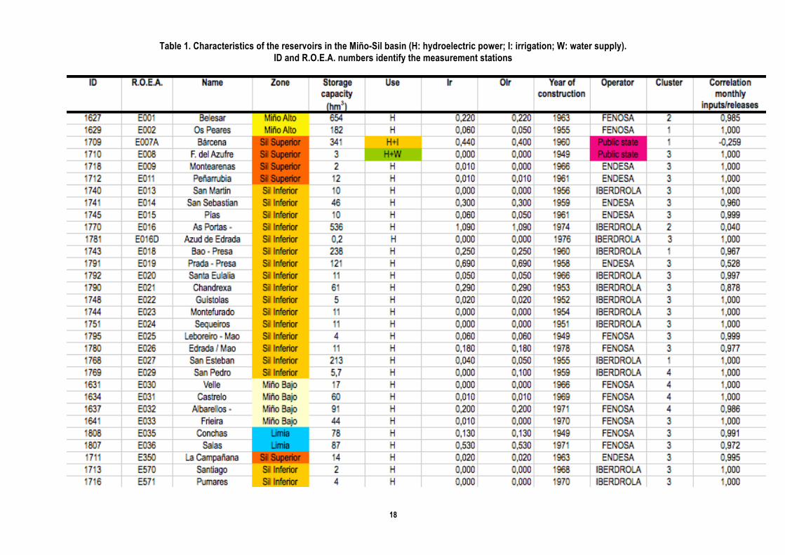
Table 1 summarizes the different characteristics of the reservoirs considered in this study, including the
impoundment ratio IR, its modified version OIR and the Pearson’s correlation coefficient between monthly
inflows and outflows. The impoundment ratio and its modified version indicate that 50% of the reservoirs
had small storage capacities to contain the long-term annual inflows, with values of less than 0.05. On the
other hand, Belesar, Bárcena, Albarellos, As Portas and Salas are among the reservoirs with higher

9
impoundment ratios ranging between 0.22 and 1.10. Furthermore, by comparing the IR and OIR values it
may be concluded that Bárcena does not reach its maximum storage capacity, because this variable is the
only difference between both quantities. It is interesting to note that three of the five reservoirs are
managed by the same company (Fenosa). Table 1 indicates also that the majority of the reservoirs with
the lowest change in flow regimes tended to have lower levels of regulation. In fact, 11 of the 36 reservoirs
studied have values of IR and OIR equal to zero, meaning that their storage capacity is extremely low in
relation to their inflow, and the correlation between inflows and outflows is 1.0 in all cases. Ten of these
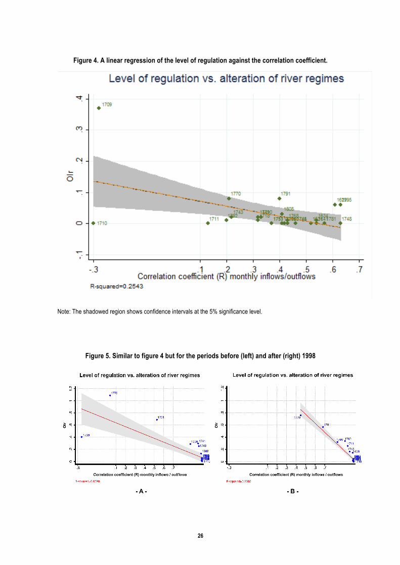
eleven reservoirs are in the same cluster (see section 3.3 and table 1). Figure 4 clearly depicts these
characteristics and shows how the Bárcena reservoir (id. 1709), which is used for both irrigation and
electricity generation, has a high level of regulation. Most of the others lie on or near the regression line.
The two panels of Figure 5 represent the level of regulation versus the alteration of reservoir regimes for
two different time periods pre- and post-liberalization (before and after 1998) of the energy market in
Spain. The post-liberalization period is characterized by a better fit between the correlation coefficient and
the OIR than the previous period (Rpre2=0.61; Rpost2=0.90). The low value of the correlation coefficient
for the As Portas reservoir (id. 1770) before 1998 indicates a significant improvement in regime after
liberalization. In contrast, the correlation coefficient of the Bárcena (1709) reservoir switched from a
negative value before 1998, indicative of an inverted flow regime downstream of the reservoir, to a positive
value (0.83) that indicates a very low change in the fluvial regime. For each of the remaining reservoirs
there was a slight change of both OIR and correlation coefficient between the two periods.
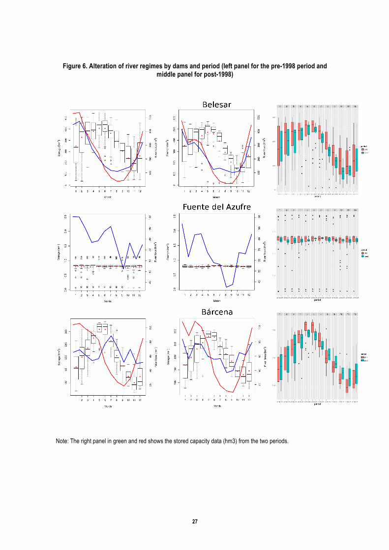
Storage capacity and flows were also assessed for both periods (see Figure 6 and dynamic content 3).
Storage capacity is conveniently represented using a box plot. For instance, the inter-quartile range (IQR)
gives a useful indication of the “spread” of the middle 50 percent of the data. Because the middle 50
percent is not affected by outliers or extreme values, this gives a more robust and less biased visualization
of the data spread. The IQR of Belesar’s storage capacity decreased after 1998 for each month of the
year, indicating a lower spread than during the previous period. The right plot provides a visual
comparison between the two panels, which indicates similar behavior for the two periods. However, both
the mean and median tend to decrease during the second period (post-1998), especially from July to
October. Further, the upper whiskers indicate that monthly maximum capacities were recorded during the
first period. The bottom whiskers for the months September to December are lower in the second period
than the first, while greater in the second period for the other months (they are very similar in March).
Thus, there is an indication of storage capacity difference between the two periods for at least 7 months of
the year. Furthermore, although the maximum values of storage capacity were recorded during the first
period, the minimum values were also recorded in the same period for the months from January to August.
The effect of market liberalization is clear in the reservoirs corresponding to the Miño-Bajo zone. Before
1998 the reservoirs in this region were operated using maximum storage criteria to maximize power

10
production. Moreover Albarellos is now operated using a maximum capacity 10 hm3 lower, in order to
avoid inundations in its region of influence. As far as flows are concerned, the general shapes did not
change between the periods, suggesting that the fluvial regime and intraannual conditions upstream were
themselves unchanged.
The box plot representation shows the changes in the storage capacity of Fuente del Azufre reservoir (as
in Figure 3 the blue line overlaps red line). The box size shows that the data are less dispersed in the
second period than the first, and the medians also tend to decrease during the second period (post-1998),
especially during the winter season. In other words, storage capacity decreased during the second period
for 9 months of the year. Despite this decline in storage capacity, the whiskers show that minimum
capacity values were recorded in the first period for almost every month of the year. Similarly, the pattern
of the flows changed between the two periods, suggesting a relative fall in flows during the summer
season.
In the same manner, the box plot representations of Barcena’s storage capacity during the second period
depicts a fall from April to July and an increase from October to December. The upper whiskers show that
maximum storage capacity values were higher in the first period for January to July but lower for
September to December. The lower whiskers of the months March to June were higher in the first period,
whereas those for the rest of the year were higher in the second period.
The position of the median is in most cases indicative of a clear skewness of the data and suggests the
use of statistical tests that relax the normality assumption. In the next section the Mann Kendall non-
parametric (MK) test is applied to assess trends in the storage capacity and flows, with the two periods of
the study assessed separately.
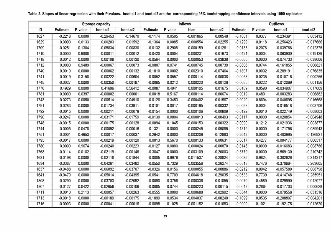
3.2. Trend analysis For monthly storage capacity, linear regression results in significant trends for 72% of the cases, of which
17 reservoirs have negative trends and 4 reservoirs have positive trends. In the Sil-inferior zone, 9 of the
16 reservoirs considered have significant negative trends, as do all four reservoirs in the Miño-Bajo zone.
These results are confirmed in most cases by the MK test, as indicated by the Kendall rank correlation
coefficients (τ), and the corresponding p-values and bootstrapping confidence intervals (see Tables 2 and
3).
For monthly outflows, linear regression indicates significant negative trends in 52% of cases. For instance,
all reservoirs in the Sil-superior zone have a significant negative trend, which is corroborated by the non-

11
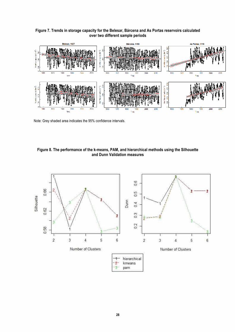
parametric MK test. Figure 7 shows the linear regression trends of storage capacity for three important
reservoirs in the Miño-Sil basin (for plots of other reservoirs see dynamic content 4). By selecting different
sample periods, persistent negative trends in storage capacity are shown for the Belesar and Bárcena
reservoirs, while As Portas shows a significant positive trend.
A two-period analysis was performed to assess the different trends during the periods before and after
1998. Table 4 provides a concise account of the change in seasonal trends for storage capacity and flows.
In summary, the main changes occurred during the summer season, especially for inflows and outflows.
The most striking finding is the increased number of statistically significant negative trends in both inflow
and outflow in the August of the second period. The significant positive trends in both inflow and outflow in
June of the first period have almost vanished during the second period. Similarly in January, an increased
number of significant negative trends was recorded in the second period. Periods of positive trends also
changed between the periods. For instance, the number of significant positive trends in storage capacity
decreased in 8 months of the year, with the most frequent changes occurring in the Sil superior zone,
followed by Miño Alto zone.
Interestingly, it is only in November that there are more reservoirs with positive trends in storage capacity
than reservoirs with negative trends.
In winter, there are at most four reservoirs with positive trends in storage capacity, which occurred for
February before 1998: after 1998, such a trend is only obtained for one reservoir. In general, negative
storage trends are more common than positive ones. For 7 months of the year they are more common
than positive ones when considering the 'whole sample'. Before 1998, six months show a greater number
of reservoirs with negative trends compared to four months where reservoirs with positive trends were in
the majority.
After 1998, the numbers for trends in storage capacity are almost the same, with six months
predominantly negative and five positive. Moreover for April and May there are eight reservoirs that show
positive trends and eight with negative trends respectively. This compares to one and zero for the opposite
trends in the same months. For the summer months this same relationship is 4-1, 0-5 and 10-1 for
negative and positive trends, respectively. This suggests that the pattern is at least partly caused by the
regulation of flow by dams, where in a given month a dam stores a great amount of water, which is used to
generate hydropower before passing to the next reservoir downstream.
The greatest numbers of trends in storage capacity are related to high numbers of trends in inflows and
outflows, always maintaining the sign of the trend. For example, in post-1998 January there is a negative
trend in storage capacity for 13 reservoirs. This number matches a negative trend in the inflow for 12

12
reservoirs and outflow for 18. A similar behavior can be observed for August and for the whole sample for
May and December. For positive trends such a link is only obvious for April post-1998.
3.3. Cluster analysis Clustering methods are very useful to find common patterns in different data series. Several of them are
commonly used in hydrological research. Each method has benefits and limitations and it can be hard to
determine a priori which is the best one for a given study. Here a number of different clustering methods
were used for the analysis in order to get a wider perspective of the studied problem and a more robust
result. The data set of measurements used so far was extended by adding the monthly MK coefficients
calculated in the previous section. Table 5 gives the average values of cluster validation indexes
calculated by the clustering methods applied in this study. The distance-based measurements include the
following: cluster separation (btwn); the average distances within clusters (avg within); and the average
distances between clusters. Other indices considered include the Silhouette index and the Dunn index.
The Dunn Index values were more varied across the cluster number domain, but in general the k-means
and hierarchical clustering techniques showed the highest values, and were therefore chosen as the
preferred techniques. Figure 8 plots the Dunn Index and Silhouette width as two measures of cluster
number validation. Remembering that both the Dunn Index and the Silhouette Width should be maximized
to obtain the optimum number of clusters, it appears that the hierarchical clustering and k-means methods
perform better than the PAM method under the Dunn Index or the Silhouette width, if the number of
clusters is greater than three. There are therefore 2 or 4 possible clusters. However, because 2 clusters
might be insufficient to extract optimal information from the data, we opted for 4 clusters, which is highly
recommended by the Dunn Index validation theory.
Looking at Table 5 it appears that storage capacity was the main factor in the cluster groupings. Cluster 1
is composed of Os Peares, Bárcena, Bao and San Esteban (see Table 1) which are reservoirs with
storage capacities between 182 and 341 hm3. All the reservoirs in this cluster have significant negative
trends, apart from Os Peares which has a positive trend. The corresponding outflows show significant
negative trends for Bárcena and San Esteban only. Cluster 2 contains reservoirs with high storage
capacities, on average almost twice those of the first cluster. Neither of the reservoirs in this cluster have
any significant trend in outflow but show opposite trends in storage capacity, with As Portas having a
positive trend. Cluster 3 contains most of the reservoirs considered in this study, but does not show any
clear-cut characteristics, even though all the reservoirs in the Sil-inferior zone belonging to cluster 3, apart
from San Martin, have significant negative trends for both storage capacity and outflow. Finally, all the
reservoirs in cluster 4 are in the Miño-bajo zone and show significant negative trends for storage capacity.
It is worth noting that the Montearenas, As Portas, San Martin, and Os Peares reservoirs have significant

13
positive trends, very pronounced in the case of As Portas and Montearenas (see figure 7 and dynamic
content 4).
4. Discussion In this study we used the operational impoundment ratio, and the degree of correlation between monthly
inflows and outflows, to assess the hydrological alterations and control of river flow in the Miño-Sil basin.
The different values of the Pearson’s correlation coefficient indicate that the reservoirs were subject to
varying management strategies, due in part to the liberalization of the Spanish energy market in 1998 and
the consequent management strategies of private companies. In effect, the effect on monthly flows ranged
from practically no change in regime to compete inversion in seasonal pattern, due to extra outflows for
irrigation in summer. The correlation between inflows and outflows ranged from 0.91 to 1 for the former
type of reservoirs and from 0.027 to 0.333 for the latter. This is in fact a common characteristic of many
reservoirs in the Mediterranean region, exemplified by the Spanish reservoirs [Batalla et al. 2004;
Goodess and Jones 2002; Philandras et al. 2011].
It is possible that the post-1998 changes in reservoir regimes (storage, inflows and outflows) could be
related to the impacts of climate change, but this is an issue to be addressed in future research.
There is a relationship between the operational impoundment ratio and the river’s degree of alteration, in
the sense that reservoirs with low change of flow regimes tend to be lightly regulated.
The use of a reservoir also affects the degree to which flow regimes are altered. It is of interest to highlight
two contrasting characteristics: 1) reservoirs intended to produce only hydroelectricity have small values of
operational impoundment ratio and are subject to minimal regime alterations, 2) reservoirs designed to
supply multiple uses, such as hydropower generation and irrigation, have greater impoundment ratios and
are prone to greater regime change.
For the period studied, 86% of the 30 reservoirs studied were affected by decreasing inflows, a feature
that also transmitted in most cases to lower storage capacity of the reservoirs. It is clear that how the
inflows and outflows are managed has a direct impact on a reservoir’s storage capacity. For instance, for
all the reservoirs located in the Baixo-Miño zone, close to the river mouth, negative trends are detected for
both flows and storage capacity. In the Sil-inferior zone where most of the reservoirs are located, 10 of the
16 reservoirs have negative trends in both storage capacity and inflow. Seasonal analysis of the trends
also reveals important findings. The inflows of all the reservoirs show a negative trend for more than 36%
of the cases in March, May, September and October. By contrast, 8 of the 30 reservoirs show a positive

14
trend in April (36% of the cases). In other words, and taking 36% as an example of the percentage
occurrence, seasonal negative trends are more common than seasonal positive trends.
The cluster analysis yields a first group (Cluster 1) comprising Os Peares, Bárcena, Bao and San
Esteban, which are reservoirs with storage capacity between 182 and 341 hm3. Except for Os Peares
which has a positive trend, all the reservoirs in this cluster have significant negative trends. The
corresponding inflows exhibited significant negative trends for all except the Bao reservoir. Cluster 2
comprises the Belesar and As Portas reservoirs, which are the most important in terms of capacity.
Belesar, the largest, shows a significant negative trend in storage, inflows and inflows. As Portas has had
a significant increase in its storage capacity in the face of declining inflows, particularly in the spring
season during the study period. This has been achieved by managing the reservoir’s outflows to offset the
negative impact of the dropping inflows on storage capacity. As Portas has a system installed to pump
outflows back to the reservoir to improve both management and economic benefit. Cluster 3 contains most
of the reservoirs, accounting for 21 of the total of 30. Significant negative trends in inflow were detected for
18 of these reservoirs, which have in turn been directly affecting the storage capacity for 10 of those
reservoirs. On the other hand, the Montearenas, San Martin and Prada reservoirs have shown significant
positive trends during the period of study, which is simply due to a management strategy that controls
flows to maintain maximum storage. Cluster 4 comprises three reservoirs in the Miño-Bajo zone with
storage capacities ranging between 17 and 91 hm3. During the period of study, each of these reservoirs
showed negative trends for storage capacity, inflow and outflow, with a particular decline in inflow during
spring and autumn.
15
References
Añel, J. A. (2011), The importance of reviewing the code. Communications of the ACM. 54 (5), doi: 10.1145/1941487.1941502.
Barlett, R., Baker, J., Lacombe, G., Doungsavanh, S., Jeuland, M. (2012), Analyzing economic tradeoffs of water use in the Nam Ngum river basin, Lao PDR. Duke Environmental Economics Working Paper EE12-10
Batalla, R. J., Gómez, C. M., and Kondolf, G. M. (2004), Reservoir-induced hydrological changes in the Ebro River basin (NE Spain). J Hydrol 290(1–2):117–136.
Bates, B. C., Kundzewicz Z. W., Wu, S., Palutikof, J. P., eds. (2008), Climate Change and Water. Geneva: IPCC Secretariat. pp 210.
Bonell, M., and Summer, G. (1992), Autumn and winter daily precipitation areas in Wales, 1982-1983 to 1986-1987. Int J Climatol 12(1):77-102.
Botter, G., Basso, S., Porporato, A., Rodríguez-Iturbe, I., Rinaldo, A. (2010), Natural streamflow regime alterations: damming of the Piave river basin (Italy), Water Resources Research 46 (6).
Cleveland, W. S., Grosse E., and Shyu, W. M. (1993), Local regression models. In: Chambers,J.M., Hastie, T.J.(Eds.), Statistical models in S.Chapman & Hall, Boca Raton,Florida, pp. 309–379.
Confederación Hidrográfica del Miño-Sil (2012), Plan Hidrológico 2010-2015 de la parte española de Demarcación Hidrográfica del Miño-Sil.
Davison, A.C., and Hinkley, D.V. (1997), Bootstrap Methods and Their Application. Cambridge University Press.
Espejo, C., García-Marín, R., (2010), Agua y energía: producción hidroeléctrica en España. Investigaciones Geográficas, 51:107-129
Everitt, B. S., Landau, S., Leese, M., and Stahl, D. (2011), Cluster Analysis, Chichester, UK: John Wiley & Sons, 5th edition. Cited on p. 165, 166, 171,176, 180, 198.
Fu, G., Chen, S., Liu, C., Shepard, D. (2004), Hydro-climatic trends of the yellow river basin for the last 50 years. Clim Change 65: 149-178.
Gago, A., Labandeira, X., López-Otero, X. (2013), A panorama on energy taxes and green tax reforms. Economics for Energy WP 08/13.
García, N. O., Gimeno, L., De la Torre, L., Nieto, R., Añel, J. A. (2005), North Atlantic Oscillation (NAO) and precipitation in Galicia (Spain), Atmósfera, 18: 25-32.
García, A., Jorde, K., Habit, E., Caamaño, D., Parra, O. (2011), Downstream environmental effects of dam operations: changes in habitat quality for native fish species, River Research and Implications 27 (3):312-327
Gimeno, L., Añel, J. A., González, H., Ribera, P., García, R., Hernández, E. (2001), The Temperature Component of the Common-Sense Index in Northwestern Iberian Peninsula. In Brunet-India M and López-Bonillo D (eds) Detecting and Modelling Regional Climate Change. Springer, Berlin, pp 143-151.
Goodess, C. M., Jones, P. D., (2002), Links between circulation and changes in the characteristics of Iberian rainfall. Int J Climatol, 22:1593–1615. doi: 10.1002/joc.810.
Gordon, A. D. (1987), A review of hierarchical classication. J R Stat Soc A Stat, 150, 119-137. Cited on p. 165.
Hamed, K. H. (2008), Trend detection in hydrological data: The Mann-Kendall trend test under the scaling hypothesis. J Hidrol, 349, 350-363. doi:10.1016/j.jhydrol.2007.11.009.
Hamududu, B., Killingtveit, A. (2012), Assessing Climate Change Impacts on Global Hydropower. Energies, 5(2), 305-322; doi:10.3390/en5020305.

16
Iimi, A. (2007), Estimating Global Climate Change Impacts On Hydropower Projects : Applications In India, Sri Lanka And Vietnam. In Policy Research Working Papers, The World Bank, 40 pp. Doi: 10.1596/1813-9450-4344.
Intergovernmental Panel on Climate Change (2011), IPCC Special Report on Renewable Energy Sources and Climate Change Mitigation. Prepared by Working Group III of the Intergovernmental Panel on Climate Change [O. Edenhofer, R. Pichs-Madruga, Y. Sokona, K. Seyboth, P. Matschoss, S. Kadner, T. Zwickel, P. Eickemeier, G. Hansen, S. Schlömer, C. von Stechow (eds)]. Cambridge University Press, Cambridge, United Kingdom and New York, NY, USA, 1075 pp.
Intergovernmental Panel on Climate Change (2013), Approved Summary for Policymakers of full draft report of Climate Change 2013: Physical Science Basis, Stocker T, Dahe Q, Plattner G-K, coordinating lead authors, available: http://www.ipcc.ch/report/ar5/wg1.
Kendall, M.G., (1975), Rank correlation methods, 4th ed. Charles Griffin, London.
Lehner, B., Czisch, G., & Vassolo, S. (2005), The impact of global change on the hydropower potential of Europe: a model-based analysis. Energy Policy 33(7): 839–855.
López-Moreno, J.I., Beguería, S., García-Ruiz, J.M. (2002), Influence of the Yesa reservoir on floods of the Aragón River, central Spanish Pyrenees, Hydrology and Earth System Sciences 6(4):752-763.
López-Moreno, J.I., Vicente-Serrano, S.M., Beguería, S., García-Ruiz, J.M., Portela, M.M., Almeida, A.B. (2009), Dam effects on droughts magnitude and duration in a transboundary basin: the lower river Tagus, Spain and Portugal, Water Resources Research 45(2).
Lorenzo-Lacruz, J., Vicente-Serrano, S. M., López-Moreno, J. I., Morán-Tejeda, E., Zabalza, J. (2012), Recent trends in Iberian streamflows (1945–2005), J. Hydrology, 414–415, 463-475. doi:10.1016/j.jhydrol.2011.11.023.
Mann, H.B. (1945), Nonparametric tests against trend. Econometrica 13: 245-259.
Martin, J.L., McCutcheon, S.C., Schottman, R.W. (1999). Hydrodynamics and transport for water quality modeling. Lewis Publishers, Boca Raton.
Martínez-Gil, F. J., Soto Castiñeira, M. (2006), O tempo dos ríos, Universidade da Coruña, A Coruña. 356 pp.
Ministerio de Asuntos Exteriores y de Cooperación (2010), Protocolo de revisión del convenio sobre cooperación para la protección y aprovechamiento sostenible de las aguas de las cuencas hidrográficas hispano-portuguesas y el protocolo adicional, suscrito en Albufeira el 30 de noviembre de 1998. BOE(14), 3425-3432.
Moberg, A., and Jones, P. D. (2005), Trends in indices for extremes in daily temperature and precipitation in central and western Europe, 1901–99. International Journal of Climatology 25(9):1149-1171.
Morán-Tejeda, E., Lorenzo-Lacruz, J., López-Moreno, J. I., et al. (2012), Reservoir Management in the Duero Basin (Spain): Impact on River Regimes and the Response to Environmental Change. Water Resources Management. doi: 10.1007/s11269-012-0004-6.
Mukheibir, P. (2013), Potential consequences of projected climate change impacts on hydroelectricity generation. Clim Change 121(1):67-78. doi: 10.1007/s10584-013-0890-5.
Philandras, C.M., Nastos, P.T., Kapsomenakis, J., et al. (2011), Long term precipitation trends and variability within the Mediterranean region. Nat Hazards Earth Syst Sci, 11:3235–3250. doi: 10.5194/nhess-11-3235-2011.
R Core Team (2012), R: A Language and Environment for Statistical Computing. R Foundation for Statistical Computing, Vienna, Austria.
Renöfalt, B.M., Jansson, R., Nilsson, C. (2010), Effects of hydropower generation and opportunities for environmental flow management in Swedish riverine ecosystems, Freshwater Biology 55 (1):49-67.
Ripley, B. D. (2002) Statistical Data Mining: http://www.stats.ox.ac.uk/pub/bdr/SDM2002/DM2002.pdf

17
Rotstayn, L. D., and Lohmann, U. (2002), Tropical rainfall trends and the indirect aerosol effect. Journal of Climate 15(15):2103-2116.
Tanaka, S. T., Zhu, T., Lund, J. R., Howitt, R. E., Jenkins, M. W., Pulido, M. A., Tauber, M. E., Ritzema, R. S., Ferreira, I. C. (2006), Climate warming and water management adaptation for California. Clim Change 76(3–4):361– 387.
Trigo, R. M. (2011), The Impacts of the NAO on the Hydrology of the Eastern Mediterranean, in Hydrological, Socioeconomic and Ecological Impacts of the North Atlantic Oscillation in the Mediterranean Region, edited by S. M. Vicente-Serrano and R. M. Trigo, pp. 41 – 56, Springer.
Ward, J. H. Jr. (1963), Hierarchical Grouping to Optimize an Objective Function, Journal of the American Statistical Association 58:236–244.
Yin, X., Yang, Z., Petts, G. (2011), Reservoir operating rules to sustain environmental flows in regulated rivers, Water Resources Research 47(8).
Zhang, Q., Xu, C-Y., Gemmer, M., Chen, Y-D., Liu, C. (2009), Changing properties of precipitation concentration in the Pearl River basin, ChinaStoch. Environ. Res. Risk Assess. 23:377-385. doi: 0.1007/s00477-0080225-7.
Zhao, Y. (2013), R and Data Mining: Examples and Case Studies. Academic Press.
18
Table 1. Characteristics of the reservoirs in the Miño-Sil basin (H: hydroelectric power; I: irrigation; W: water supply). ID and R.O.E.A. numbers identify the measurement stations
19
Table 2. Slopes of linear regression with their P-values. boot.ci1 and boot.ci2 are the corresponding 95% bootstrapping confidence intervals using 1000 replicates
Storage capacity Inflows Outflows ID Estimate P-value boot.ci1 boot.ci2 Estimate P-value bias boot.ci2 Estimate P-value boot.ci1 boot.ci2
1627 -0.2218 0.0000 -0.29453 -0.14670 -0.1174 0.0505 -0.001865 0.00548 -0.1061 0.0377 -0.234391 0.003412 1629 0.0090 0.0133 0.00203 0.01592 -0.1364 0.0085 -0.000554 -0.02255 -0.1299 0.0118 -0.256423 -0.017666 1709 -0.0251 0.1384 -0.05834 0.00830 -0.0132 0.2908 0.000159 0.01261 -0.0133 0.2076 -0.039768 0.012375 1710 0.0000 0.9888 -0.00011 0.00012 -0.0420 0.0004 -0.000231 -0.01973 -0.0421 0.0004 -0.063900 -0.019129 1718 0.0012 0.0000 0.00108 0.00130 -0.0564 0.0000 0.000053 -0.03838 -0.0565 0.0000 -0.074733 -0.038006 1712 0.0000 0.9489 -0.00067 0.00073 -0.0807 0.0741 -0.000745 0.00739 -0.0806 0.0744 -0.161855 0.006821 1740 0.0010 0.0000 0.00062 0.00132 -0.1810 0.0002 0.002310 -0.07464 -0.1807 0.0002 -0.289191 -0.076835 1741 0.0019 0.3158 -0.00222 0.00604 -0.0052 0.0557 0.000114 0.00038 -0.0053 0.0235 -0.010716 0.000256 1745 -0.0027 0.0000 -0.00350 -0.00187 -0.0065 0.0212 0.000220 -0.00126 -0.0065 0.0222 -0.012069 -0.001156 1770 0.4929 0.0000 0.41696 0.56412 -0.0087 0.4941 0.000105 0.01675 0.0189 0.0590 -0.034907 0.017009 1781 0.0000 0.6397 -0.00002 0.00001 0.0018 0.5167 0.000114 0.00674 0.0019 0.4801 -0.003283 0.006882 1743 0.0273 0.0050 0.00514 0.04910 -0.0126 0.3453 -0.000402 0.01567 -0.0020 0.8694 -0.040695 0.016668 1791 0.0283 0.0000 0.01734 0.03911 -0.0101 0.0017 -0.000195 -0.00332 -0.0098 0.0004 -0.016518 -0.003706 1792 -0.0015 0.0000 -0.00211 -0.00078 -0.0154 0.0000 -0.000106 -0.00809 -0.0122 0.0010 -0.022749 -0.008003 1790 -0.0247 0.0000 -0.03171 -0.01759 -0.0130 0.0004 -0.000013 -0.00493 -0.0117 0.0000 -0.020854 -0.004948 1748 -0.0015 0.0000 -0.00175 -0.00128 -0.0094 0.1045 -0.000153 0.00322 -0.0090 0.1212 -0.021936 0.003877 1744 -0.0005 0.0478 -0.00092 -0.00016 -0.1321 0.0000 0.000245 -0.09085 -0.1319 0.0000 -0.171756 -0.089943 1751 0.0001 0.4653 -0.00017 0.00037 -0.2642 0.0000 0.003206 -0.12883 -0.2642 0.0000 -0.403995 -0.126921 1795 -0.0017 0.0000 -0.00219 -0.00120 0.0013 0.5670 0.000133 0.00631 0.0017 0.4277 -0.004177 0.006517 1780 0.0000 0.9674 -0.00240 0.00223 -0.0127 0.0000 0.000024 -0.00870 -0.0145 0.0000 -0.016683 -0.008786 1768 -0.0114 0.0182 -0.02119 -0.00146 -0.3847 0.0000 -0.003109 -0.20003 -0.3779 0.0000 -0.569130 -0.210742 1631 -0.0198 0.0000 -0.02118 -0.01844 -0.0005 0.9976 0.011537 0.28824 0.0035 0.9824 -0.302626 0.314217 1634 -0.0387 0.0000 -0.04261 -0.03482 -0.0550 0.7329 0.003556 0.26274 -0.0518 0.7476 -0.370664 0.263605 1637 -0.0488 0.0000 -0.06092 -0.03707 -0.0326 0.0156 0.000055 -0.00886 -0.0212 0.0942 -0.057580 -0.008798 1641 -0.0470 0.0000 -0.05014 -0.04395 -0.0541 0.7709 0.004618 0.29035 -0.0533 0.7739 -0.414748 0.285951 1808 -0.0290 0.0000 -0.03703 -0.02092 -0.0090 0.3756 0.000336 0.01055 -0.0070 0.4589 -0.029990 0.012077 1807 -0.0127 0.0422 -0.02656 0.00106 -0.0085 0.0744 -0.000223 0.00115 -0.0043 0.2864 -0.017703 0.000628 1711 0.0010 0.2113 -0.00057 0.00263 -0.0555 0.0000 -0.000688 -0.02992 -0.0544 0.0000 -0.079558 -0.031516 1713 -0.0018 0.0000 -0.00189 -0.00175 -0.1099 0.0534 -0.004037 -0.00240 -0.1099 0.0535 -0.208807 -0.004201 1716 -0.0003 0.0000 -0.00041 -0.00016 -0.0898 0.1028 -0.001152 0.01683 -0.0900 0.1021 -0.192175 0.012620

20
Table 3. Mann-Kendall tests with their P-values. Bootstrapping confidence intervals as in Table 2
Storage Capacity Inflows Outflows
ID tau P-value boot.ci1 boot.ci2 tau P-value boot.ci1 boot.ci2 tau P-value boot.ci1 boot.ci2 1627 -0.2198 0.0000 -0.554688 -0.31737 -0.1298 0.0000 -0.35784 -0.15926 -0.0786 0.0044 -0.25958 -0.051086 1629 0.1651 0.0000 0.222811 0.43407 -0.0523 0.0465 -0.19326 -0.01405 -0.0461 0.0789 -0.18999 0.005318 1709 -0.1007 0.0002 -0.295250 -0.11110 -0.1313 0.0000 -0.36316 -0.16598 -0.0853 0.0020 -0.25424 -0.083249 1710 -0.0601 0.0278 -0.257487 0.02203 -0.1529 0.0000 -0.40462 -0.20975 -0.1528 0.0000 -0.40345 -0.200560 1718 0.4890 0.0000 0.828256 1.13726 -0.4172 0.0000 -0.98074 -0.68743 -0.4167 0.0000 -0.98399 -0.677259 1712 -0.0174 0.5541 -0.125579 0.05817 -0.1644 0.0000 -0.42869 -0.21886 -0.1625 0.0000 -0.42604 -0.217505 1740 0.1112 0.0000 0.119786 0.33256 -0.1516 0.0000 -0.39570 -0.21299 -0.1504 0.0000 -0.39653 -0.212008 1741 0.0169 0.5272 -0.064309 0.13950 -0.0906 0.0007 -0.25602 -0.10804 -0.1048 0.0001 -0.28847 -0.132313 1745 -0.2952 0.0000 -0.734945 -0.43449 -0.1144 0.0000 -0.31128 -0.14695 -0.1120 0.0000 -0.30560 -0.140987 1770 0.3805 0.0000 0.579937 0.94017 -0.0489 0.1184 -0.22690 0.02907 0.0353 0.2605 -0.03814 0.173329 1781 -0.0640 0.0614 -0.229388 -0.03433 0.0374 0.2742 -0.01429 0.17034 0.0350 0.3057 -0.01389 0.157755 1743 -0.0189 0.4813 -0.130027 0.05766 0.0400 0.1348 -0.01440 0.18108 0.0174 0.5155 -0.04453 0.124521 1791 0.1522 0.0000 0.198009 0.41806 -0.1462 0.0000 -0.38758 -0.19571 -0.1247 0.0000 -0.32541 -0.167720 1792 -0.1309 0.0000 -0.383658 -0.13994 -0.1783 0.0000 -0.45894 -0.24245 -0.1356 0.0000 -0.36548 -0.167971 1790 -0.2371 0.0000 -0.588558 -0.35691 -0.1874 0.0000 -0.45864 -0.29275 -0.1152 0.0000 -0.30608 -0.147734 1748 -0.3385 0.0000 -0.800027 -0.54989 -0.1262 0.0000 -0.33057 -0.17321 -0.1216 0.0000 -0.31830 -0.161396 1744 -0.1418 0.0000 -0.375784 -0.18722 -0.2392 0.0000 -0.58266 -0.36389 -0.2391 0.0000 -0.58343 -0.357137 1751 -0.1903 0.0000 -0.477858 -0.2809 -0.1833 0.0000 -0.46757 -0.26026 -0.1836 0.0000 -0.47455 -0.265496 1795 -0.3059 0.0000 -0.757207 -0.47927 -0.0331 0.2843 -0.19168 0.05799 0.0135 0.6619 -0.09696 0.146389 1780 -0.0192 0.5753 -0.138786 0.07525 -0.2946 0.0000 -0.71842 -0.45036 -0.3274 0.0000 -0.81463 -0.482939 1768 -0.0516 0.0495 -0.193989 -0.02751 -0.2110 0.0000 -0.53034 -0.31974 -0.1984 0.0000 -0.50256 -0.290285 1631 -0.4735 0.0000 -1.132986 -0.76819 -0.0653 0.0285 -0.25261 -0.01642 -0.0613 0.0399 -0.24223 -0.002873 1634 -0.3887 0.0000 -0.938915 -0.60965 -0.0946 0.0015 -0.31143 -0.07581 -0.0942 0.0016 -0.30918 -0.076694 1637 -0.3078 0.0000 -0.751764 -0.47173 -0.2122 0.0000 -0.52951 -0.31741 -0.0997 0.0011 -0.28881 -0.114622 1641 -0.4324 0.0000 -1.032467 -0.70167 -0.0941 0.0016 -0.31614 -0.06304 -0.0936 0.0017 -0.30405 -0.074281 1808 -0.2765 0.0000 -0.666141 -0.43866 0.0091 0.7278 -0.07962 0.11869 -0.0400 0.1282 -0.17922 0.020938 1807 0.0365 0.2378 -0.079999 0.23499 -0.1507 0.0000 -0.41224 -0.20333 -0.0061 0.8433 -0.10874 0.084704 1711 0.0451 0.1257 -0.001923 0.17050 -0.1679 0.0000 -0.44706 -0.22853 -0.1651 0.0000 -0.42641 -0.227470 1713 -0.6252 0.0000 -1.422752 -1.07007 -0.1785 0.0000 -0.46078 -0.25291 -0.1783 0.0000 -0.46071 -0.253738 1716 -0.2737 0.0000 -0.685371 -0.41620 -0.1668 0.0000 -0.43588 -0.22501 -0.1657 0.0000 -0.43943 -0.226827

21
Table 4. Frequency of monthly trends for the whole sample, and for periods pre- and post-1998
Periods Trend Jan Feb Mar Apr May Jun Jul Aug Sep Oct Nov Dec
Whole Sample
Storage capacity
Negative Trend 4 5 4 7 12 5 8 4 3 4 3 10
Positive Trend 2 1 4 1 5 5 3 4 2 4 6 1
Inflow Negative Trend 0 1 6 2 14 3 0 1 1 6 0 14
Positive Trend 2 3 0 4 1 0 3 4 0 0 1 0
Outflow Negative Trend 1 1 6 2 15 1 0 1 2 7 0 14
Positive Trend 2 4 0 5 2 0 3 2 0 0 1 0
Pre-1998
Storage capacity
Negative Trend 4 3 6 2 5 4 3 5 5 3 4 3
Positive Trend 3 4 2 1 2 6 2 5 5 6 6 0
Inflow Negative Trend 1 0 1 7 1 2 10 0 0 1 2 0
Positive Trend 0 0 4 0 2 11 0 5 0 2 3 0
Outflow Negative Trend 0 1 1 8 1 3 11 1 0 1 2 1
Positive Trend 1 2 7 0 2 13 1 5 0 2 6 0
Post-1998
Storage capacity
Negative Trend 13 2 1 1 8 4 0 10 0 0 3 2
Positive Trend 0 1 3 8 0 1 5 1 2 4 2 2
Inflow Negative Trend 12 0 0 0 2 0 0 29 0 0 1 0 Positive Trend 0 1 0 5 0 1 0 0 4 4 0 0
Outflow Negative Trend 18 0 0 1 4 1 0 27 0 0 3 0
Positive Trend 0 2 0 8 0 0 1 0 6 8 0 0
Note: Only trends that are statistically significant at the 5% level are included. Seasons are highlighted with different colors.

22
Table 5. Validation statistics calculated for the different clustering methods used.
Cluster 2 3 4 5 6 7 10 K-mean Avg within 162 108 79 56 42 52 31
Avg-btwn 547 424 392 309 308 272 267 wb ratio 0.2970 0.2557 0.2039 0.1831 0.1534 0.1462 0.1138 Avg silwidth 0.6125 0.6054 0.6670 0.5773 0.5680 0.5823 0.4746 Dunn 0.2180 0.2923 0.6645 0.2526 0.1488 0.1488 0.1207
PAM Avg within 141 91 79 56 42 34 30 Avg-btwn 1 422 391 392 309 274 273 272 wb ratio 0.3337 0.2330 0.2039 0.1831 0.1534 0.1266 0.1125 Avg silwidth 0.5973 0.6390 0.6670 0.5773 0.5847 0.5823 0.4978 Dunn 0.2829 0.2829 0.6645 0.2526 0.1488 0.2046 0.3622
Hierarchical Avg within 176 133 79 78 52 52 30 Avg-btwn 2 628 421 392 388 308 307 272 wb ratio 0.2803 0.3171 0.2039 0.2013 0.1717 0.1691 0.1125 Avg silwidth 0.6937 0.5460 0.6670 0.6449 0.5680 0.5338 0.4978 Dunn 0.4668 0.3781 0.6645 0.5302 0.3473 0.3941 0.3622
Note: Avg within: average distances within clusters; Avg-btwn: average distances between clusters; wb ratio: ratio of the average distances within to the average distances between clusters; Avg silwidth: average Silhouette width; Dunn: Dunn index.
23
Figure 1. Location of the Miño-Sil basin in the Iberian Peninsula, and reservoir locations (triangles) indicated by ID number
24
Figure 2. Temporal coverage of inflow/outflow data series for the selected reservoirs indicated by ID number
25
Figure 3. Alteration of river regimes by dams
Note: The boxplots represent the distribution of the stored capacity, the red dot inside the box is the mean, the red lines are the inflows and the blue lines are the outflows.
26
Figure 4. A linear regression of the level of regulation against the correlation coefficient.
Note: The shadowed region shows confidence intervals at the 5% significance level.
Figure 5. Similar to figure 4 but for the periods before (left) and after (right) 1998
27
Figure 6. Alteration of river regimes by dams and period (left panel for the pre-1998 period and middle panel for post-1998)
Note: The right panel in green and red shows the stored capacity data (hm3) from the two periods.
28
Figure 7. Trends in storage capacity for the Belesar, Bárcena and As Portas reservoirs calculated over two different sample periods
Note: Grey shaded area indicates the 95% confidence intervals.
Figure 8. The performance of the k-means, PAM, and hierarchical methods using the Silhouette and Dunn Validation measures